EXPLANATORY NOTES TO THE INTERIM … Covered by IMO Instruments (resolution A.749(18)). 2 Member Governments are invited to bring the annexed Explanatory Notes to the Interim

I:\CIRC\MSC\01\1227.doc

INTERNATIONAL MARITIME ORGANIZATION 4 ALBERT EMBANKMENT LONDON SE1 7SR Telephone: 020 7735 7611 Fax: 020 7587 3210

IMO

E

Ref. T1/2.04 MSC.1/Circ.1227 11 January 2007

EXPLANATORY NOTES TO THE INTERIM GUIDELINES FOR ALTERNATIVE

ASSESSMENT OF THE WEATHER CRITERION

1 The Maritime Safety Committee, at its eighty-second session (29 November to 8 December 2006), approved the Explanatory Notes to the Interim Guidelines for alternative assessment of the weather criterion, set out in the annex, aiming at providing the industry with alternative means (in particular, model experiments) for the assessment of the severe wind and rolling criterion (weather criterion), as contained in the Code on Intact Stability for all Types of Ships Covered by IMO Instruments (resolution A.749(18)). 2 Member Governments are invited to bring the annexed Explanatory Notes to the Interim Guidelines to the attention of interested parties as they deem appropriate.

***

MSC.1/Circ.1227


ANNEX EXPLANATORY NOTES TO THE INTERIM GUIDELINES FOR THE ALTERNATIVE

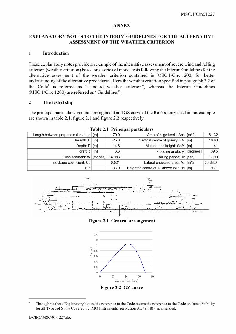
ASSESSMENT OF THE WEATHER CRITERION 1 Introduction These explanatory notes provide an example of the alternative assessment of severe wind and rolling criterion (weather criterion) based on a series of model tests following the Interim Guidelines for the alternative assessment of the weather criterion contained in MSC.1/Circ.1200, for better understanding of the alternative procedures. Here the weather criterion specified in paragraph 3.2 of the Code∗ is referred as “standard weather criterion”, whereas the Interim Guidelines (MSC.1/Circ.1200) are referred as “Guidelines”. 2 The tested ship The principal particulars, general arrangement and GZ curve of the RoPax ferry used in this example are shown in table 2.1, figure 2.1 and figure 2.2 respectively.

Table 2.1 Principal particulars Length between perpendiculars: Lpp [m] 170.0 Area of bilge keels: Abk [m^2] 61.32

Breadth: B [m] 25.0 Vertical centre of gravity: KG [m] 10.63Depth: D [m] 14.8 Metacentric height: GoM [m] 1.41

draft: d [m] 6.6 Flooding angle: φf [degrees] 39.5Displacement: W [tonnes] 14,983 Rolling period: Tr [sec] 17.90

Blockage coefficient: Cb 0.521 Lateral projected area: AL [m^2] 3,433.0 B/d 3.79 Height to centre of AL above WL: Hc [m] 9.71

Figure 2.1 General arrangement

0

0.2

0.4

0.6

0.8

1

1.2

1.4

0 20 40 60 80

Angle of Heel [deg]

GZ [m]

Figure 2.2 GZ curve

∗ Throughout these Explanatory Notes, the reference to the Code means the reference to the Code on Intact Stability

for all Types of Ships Covered by IMO Instruments (resolution A.749(18)), as amended.

MSC.1/Circ.1227 ANNEX Page 2


3 The determination of the wind heeling lever lw1 3.1 Model set-up 3.1.1 Ship model used for wind tests The model for the wind test was built following paragraph 1.2.1 of the Guidelines. The length (Lpp) of the model was 1.5 m (scale: 1/113). The lateral projected area in upright condition was 0.267 m2. Compared to the cross section of the wind tunnel (3 m in breadth and 2 m in height), the blockage ratio was 4.5%. 3.1.2 Ship model used for drifting tests The model for the drifting test was built following paragraph 1.2.2 of the Guidelines with bilge keels of greater than 10 mm in breadth. The length of the model was 2 m (scale: 1/85). 3.2 Wind tests 3.2.1 The arrangement for the wind tunnel tests is shown in figure 3.1. The connection between the model and load cell had a rotating device for testing the model in heeled conditions. In heeled conditions the height of the model was adjusted by the adjusting plate to keep the displacement constant when floating freely. The change of trim due to heel was neglected. 3.2.2 In order to keep the blockage ratio less than 5%, the floor plate was set to the same level of the floor of the tunnel. The gap between the model and the floor plate was kept within approximately 3 mm and covered by soft sheets for avoiding the effect of downflow through the gap∗.

Figure 3.1 Arrangement for wind tunnel tests

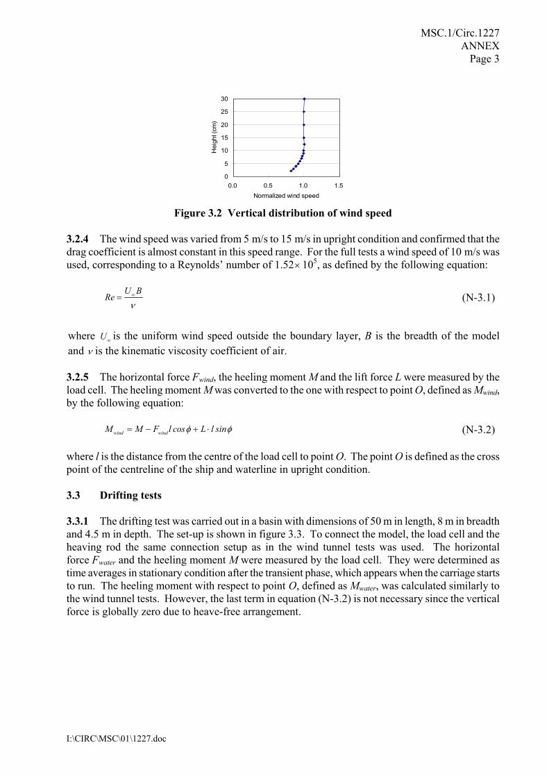
3.2.3 The vertical distribution of wind speed is shown in figure 3.2. For the test arrangement (figure 3.1), the height of the ship model from the floor was approximately 19 cm in upright condition. This means that the lower half of the model is placed in the boundary layer. The distributions of wind speed in the lateral and longitudinal directions were almost uniform (deviation less than 1%) around the model.

∗ In order to simplify the execution of the experiments and to avoid the need for the building of appropriate floor

plates for each heeling angle, the gap could be filled by water. However, in this case, if any buoyancy effect occurs in the model due to the particular setup, then it is to be properly accounted for in the subsequent analysis of the data.

MSC.1/Circ.1227 ANNEX

Page 3


0

5

10

15

20

25

30

0.0 0.5 1.0 1.5Normalized wind speed

Hei

ght (

cm)

Figure 3.2 Vertical distribution of wind speed

3.2.4 The wind speed was varied from 5 m/s to 15 m/s in upright condition and confirmed that the drag coefficient is almost constant in this speed range. For the full tests a wind speed of 10 m/s was used, corresponding to a Reynolds’ number of 1.52× 105, as defined by the following equation:

U BRe

ν∞= (N-3.1)

where U∞ is the uniform wind speed outside the boundary layer, B is the breadth of the model and ν is the kinematic viscosity coefficient of air. 3.2.5 The horizontal force Fwind, the heeling moment M and the lift force L were measured by the load cell. The heeling moment M was converted to the one with respect to point O, defined as Mwind, by the following equation:

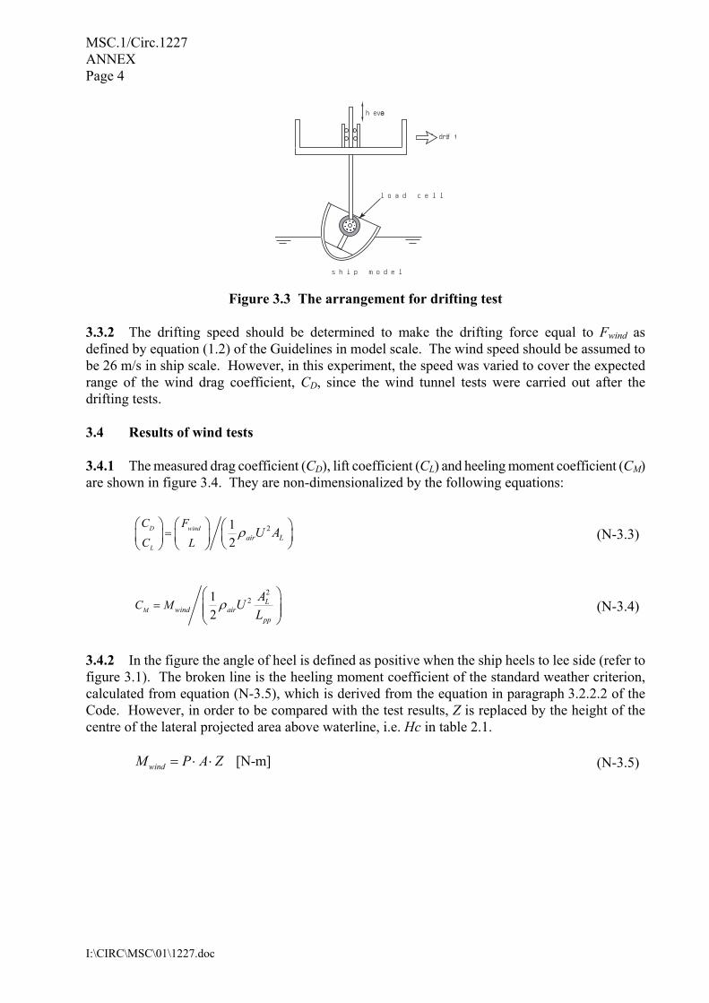
wind windM M F l cos L l sinφ φ= − + ⋅ (N-3.2) where l is the distance from the centre of the load cell to point O. The point O is defined as the cross point of the centreline of the ship and waterline in upright condition. 3.3 Drifting tests 3.3.1 The drifting test was carried out in a basin with dimensions of 50 m in length, 8 m in breadth and 4.5 m in depth. The set-up is shown in figure 3.3. To connect the model, the load cell and the heaving rod the same connection setup as in the wind tunnel tests was used. The horizontal force Fwater and the heeling moment M were measured by the load cell. They were determined as time averages in stationary condition after the transient phase, which appears when the carriage starts to run. The heeling moment with respect to point O, defined as Mwater, was calculated similarly to the wind tunnel tests. However, the last term in equation (N-3.2) is not necessary since the vertical force is globally zero due to heave-free arrangement.



load cell

ship model

heave

drift

Figure 3.3 The arrangement for drifting test 3.3.2 The drifting speed should be determined to make the drifting force equal to Fwind as defined by equation (1.2) of the Guidelines in model scale. The wind speed should be assumed to be 26 m/s in ship scale. However, in this experiment, the speed was varied to cover the expected range of the wind drag coefficient, CD, since the wind tunnel tests were carried out after the drifting tests. 3.4 Results of wind tests 3.4.1 The measured drag coefficient (CD), lift coefficient (CL) and heeling moment coefficient (CM) are shown in figure 3.4. They are non-dimensionalized by the following equations:

212

D wind

Lair L

C FC L

U Aρ=

(N-3.3)

221

2ML

wind airpp

C MAUL

ρ=

(N-3.4)

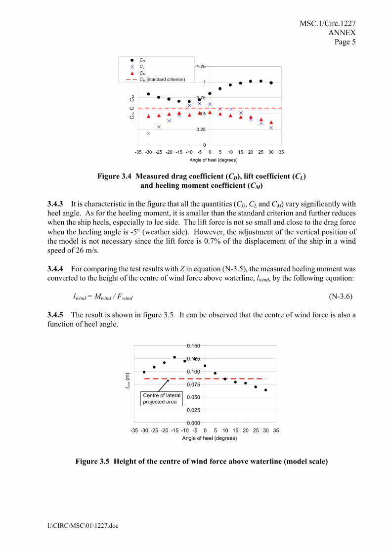
3.4.2 In the figure the angle of heel is defined as positive when the ship heels to lee side (refer to figure 3.1). The broken line is the heeling moment coefficient of the standard weather criterion, calculated from equation (N-3.5), which is derived from the equation in paragraph 3.2.2.2 of the Code. However, in order to be compared with the test results, Z is replaced by the height of the centre of the lateral projected area above waterline, i.e. Hc in table 2.1.

[N-m]windM P A Z= ⋅ ⋅ (N-3.5)


Page 5


Figure 3.4 Measured drag coefficient (CD), lift coefficient (CL)

and heeling moment coefficient (CM) 3.4.3 It is characteristic in the figure that all the quantities (CD, CL and CM) vary significantly with heel angle. As for the heeling moment, it is smaller than the standard criterion and further reduces when the ship heels, especially to lee side. The lift force is not so small and close to the drag force when the heeling angle is -5° (weather side). However, the adjustment of the vertical position of the model is not necessary since the lift force is 0.7% of the displacement of the ship in a wind speed of 26 m/s. 3.4.4 For comparing the test results with Z in equation (N-3.5), the measured heeling moment was converted to the height of the centre of wind force above waterline, lwind, by the following equation:

lwind = Mwind / Fwind (N-3.6) 3.4.5 The result is shown in figure 3.5. It can be observed that the centre of wind force is also a function of heel angle.

Figure 3.5 Height of the centre of wind force above waterline (model scale)

0

0.25

0.5

0.75

1

1.25

-35 -30 -25 -20 -15 -10 -5 0 5 10 15 20 25 30 35 Angle of heel (degrees)

CD CL CM CM (standard criterion)

CD, C

L, C

M

0.000

0.025

0.050

0.075

0.100

0.125

0.150

-35 -30 -25 -20 -15 -10 -5 0 5 10 15 20 25 30 35 Angle of heel (degrees)

l wind

(m)

Centre of lateral projected area



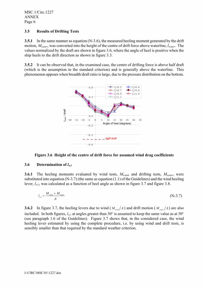
3.5 Results of Drifting Tests 3.5.1 In the same manner as equation (N-3.6), the measured heeling moment generated by the drift motion, Mwater, was converted into the height of the centre of drift force above waterline, lwater. The values normalized by the draft are shown in figure 3.6, where the angle of heel is positive when the ship heels to the drift direction as shown in figure 3.3. 3.5.2 It can be observed that, in the examined case, the centre of drifting force is above half draft (which is the assumption in the standard criterion) and is generally above the waterline. This phenomenon appears when breadth/draft ratio is large, due to the pressure distribution on the bottom.

Figure 3.6 Height of the centre of drift force for assumed wind drag coefficients

3.6 Determination of lw1 3.6.1 The heeling moments evaluated by wind tests, Mwind, and drifting tests, Mwater, were substituted into equation (N-3.7) (the same as equation (1.1) of the Guidelines) and the wind heeling lever, lw1, was calculated as a function of heel angle as shown in figure 3.7 and figure 3.8.

wind waterw1

M Ml

∆+

=

(N-3.7)

3.6.2 In figure 3.7, the heeling levers due to wind ( windM ∆ ) and drift motion ( waterM ∆ ) are also included. In both figures, lw1 at angles greater than 30° is assumed to keep the same value as at 30° (see paragraph 1.6 of the Guidelines). Figure 3.7 shows that, in the considered case, the wind heeling lever estimated by using the complete procedure, i.e. by using wind and drift tests, is sensibly smaller than that required by the standard weather criterion.

-0.6

-0.4

-0.2

0.0

0.2

0.4

0.6

-20 -15 -10 -5 0 5 10 15 20 25 30 35Angle of heel (degrees)

CD=0.5 CD=0.6CD=0.7 CD=0.8CD=0.9 CD=1.0CD=1.1

l wat

er /

draf

t

Half draft


Page 7


Figure 3.7 Wind heeling lever, lw1, evaluated by the tests

Figure 3.8 Wind heeling lever, lw1, compared with the GZ curve 4 The determination of the roll angle 1φ 4.1 Model basin The model basin used for roll decay tests and rolling motion tests in waves was the same used for the drifting tests (50 m in length, 8 m in breadth and 4.5 m in depth). The overall length of the model (2.14 m) was small enough compared to the breadth of the basin. 4.2 Model set-up 4.2.1 The model was the same used for the drifting tests (Lpp = 2 m, scale: 1/85). It was built up to the upper vehicle deck, till which buoyancy is included in the stability calculation. The top was built open, but water did not enter into the model in waves with the largest steepness. 4.2.2 The model was ballasted to the loading condition for the ship, as shown in table 2.1. To ensure correct displacement and attitude, the colour of the model was changed between above and below the load line. The GM as measured by an inclining test was 1.67 cm, corresponding to an 0.7% error to the scaled value of the ship. The natural roll period was also measured to be 1.92 s, corresponding to an 1.2% error.

-0.05

-0.025

0

0.025

0.1

0.125

0.15

-20 -10 0 10 20 30 40

Angle of heel (degrees)

l w1 [

m]

Standard criterion Wind test Drift test Wind + Drift tests

-1

-0.5

0

0.5

1

-20 -10 0 10 20 30 40 50

Angle of heel [degrees]

GZ,

l wl [

m]

GZStandard Criterion Wind + Drift tests



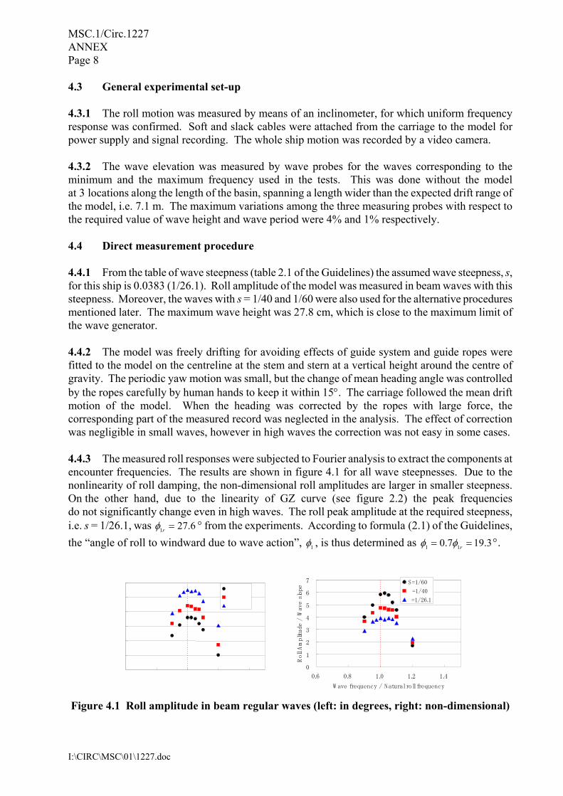
4.3 General experimental set-up 4.3.1 The roll motion was measured by means of an inclinometer, for which uniform frequency response was confirmed. Soft and slack cables were attached from the carriage to the model for power supply and signal recording. The whole ship motion was recorded by a video camera. 4.3.2 The wave elevation was measured by wave probes for the waves corresponding to the minimum and the maximum frequency used in the tests. This was done without the model at 3 locations along the length of the basin, spanning a length wider than the expected drift range of the model, i.e. 7.1 m. The maximum variations among the three measuring probes with respect to the required value of wave height and wave period were 4% and 1% respectively. 4.4 Direct measurement procedure 4.4.1 From the table of wave steepness (table 2.1 of the Guidelines) the assumed wave steepness, s, for this ship is 0.0383 (1/26.1). Roll amplitude of the model was measured in beam waves with this steepness. Moreover, the waves with s = 1/40 and 1/60 were also used for the alternative procedures mentioned later. The maximum wave height was 27.8 cm, which is close to the maximum limit of the wave generator. 4.4.2 The model was freely drifting for avoiding effects of guide system and guide ropes were fitted to the model on the centreline at the stem and stern at a vertical height around the centre of gravity. The periodic yaw motion was small, but the change of mean heading angle was controlled by the ropes carefully by human hands to keep it within 15°. The carriage followed the mean drift motion of the model. When the heading was corrected by the ropes with large force, the corresponding part of the measured record was neglected in the analysis. The effect of correction was negligible in small waves, however in high waves the correction was not easy in some cases. 4.4.3 The measured roll responses were subjected to Fourier analysis to extract the components at encounter frequencies. The results are shown in figure 4.1 for all wave steepnesses. Due to the nonlinearity of roll damping, the non-dimensional roll amplitudes are larger in smaller steepness. On the other hand, due to the linearity of GZ curve (see figure 2.2) the peak frequencies do not significantly change even in high waves. The roll peak amplitude at the required steepness, i.e. s = 1/26.1, was 1 27.6rφ = ° from the experiments. According to formula (2.1) of the Guidelines, the “angle of roll to windward due to wave action”, 1φ , is thus determined as 1 10.7 19.3rφ φ= = °.

0

1

2

3

4

5

6

7

0.6 0.8 1.0 1.2 1.4

W ave frequency / Natural roll frequency

Roll Amplitude

/ W

ave slope

S=1/60

　=1/40

=1/26.1

Figure 4.1 Roll amplitude in beam regular waves (left: in degrees, right: non-dimensional)


Page 9


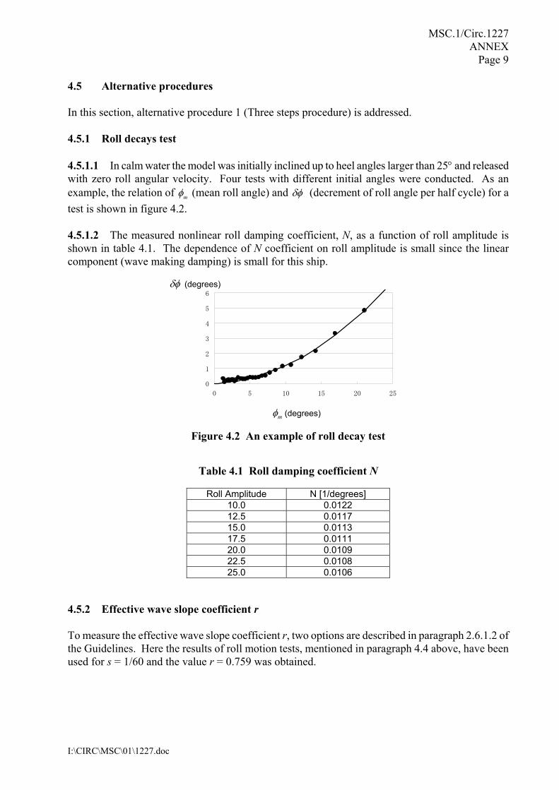
4.5 Alternative procedures In this section, alternative procedure 1 (Three steps procedure) is addressed. 4.5.1 Roll decays test 4.5.1.1 In calm water the model was initially inclined up to heel angles larger than 25° and released with zero roll angular velocity. Four tests with different initial angles were conducted. As an example, the relation of mφ (mean roll angle) and δφ (decrement of roll angle per half cycle) for a test is shown in figure 4.2. 4.5.1.2 The measured nonlinear roll damping coefficient, N, as a function of roll amplitude is shown in table 4.1. The dependence of N coefficient on roll amplitude is small since the linear component (wave making damping) is small for this ship.

0

1

2

3

4

5

6

0 5 10 15 20 25

Figure 4.2 An example of roll decay test

Table 4.1 Roll damping coefficient N

Roll Amplitude N [1/degrees] 10.0 0.0122 12.5 0.0117 15.0 0.0113 17.5 0.0111 20.0 0.0109 22.5 0.0108 25.0 0.0106

4.5.2 Effective wave slope coefficient r To measure the effective wave slope coefficient r, two options are described in paragraph 2.6.1.2 of the Guidelines. Here the results of roll motion tests, mentioned in paragraph 4.4 above, have been used for s = 1/60 and the value r = 0.759 was obtained.

mφ (degrees)

δφ (degrees)



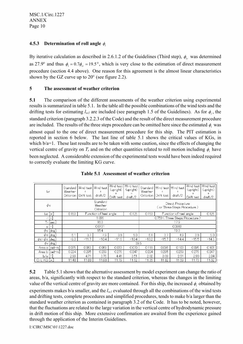
4.5.3 Determination of roll angle 1φ By iterative calculation as described in 2.6.1.2 of the Guidelines (Third step), 1rφ was determined as 27.9° and thus 1 10.7 19.5rφ φ= = °, which is very close to the estimation of direct measurement procedure (section 4.4 above). One reason for this agreement is the almost linear characteristics shown by the GZ curve up to 20° (see figure 2.2). 5 The assessment of weather criterion 5.1 The comparison of the different assessments of the weather criterion using experimental results is summarized in table 5.1. In the table all the possible combinations of the wind tests and the drifting tests for estimating lw1 are included (see paragraph 1.5 of the Guidelines). As for 1φ , the standard criterion (paragraph 3.2.2.3 of the Code) and the result of the direct measurement procedure are included. The results of the three steps procedure can be omitted here since the estimated 1φ was almost equal to the one of direct measurement procedure for this ship. The PIT estimation is reported in section 6 below. The last line of table 5.1 shows the critical values of KGs, in which b/a=1. These last results are to be taken with some caution, since the effects of changing the vertical centre of gravity on Tr and on the other quantities related to roll motion including 1φ have been neglected. A considerable extension of the experimental tests would have been indeed required to correctly evaluate the limiting KG curve.

Table 5.1 Assessment of weather criterion

5.2 Table 5.1 shows that the alternative assessment by model experiment can change the ratio of areas, b/a, significantly with respect to the standard criterion, whereas the changes in the limiting value of the vertical centre of gravity are more contained. For this ship, the increased 1φ obtained by experiments makes b/a smaller, and the lw1 evaluated through all the combinations of the wind tests and drifting tests, complete procedures and simplified procedures, tends to make b/a larger than the standard weather criterion as contained in paragraph 3.2 of the Code. It has to be noted, however, that the fluctuations are related to the large variation in the vertical centre of hydrodynamic pressure in drift motion of this ship. More extensive confirmation are awaited from the experience gained through the application of the Interim Guidelines.



6 Alternative procedure 2: Parameter identification technique (PIT) 6.1 Introduction 6.1.1 The PIT technique is a general methodology for the determination of the numerical values for a certain number of parameters in a given analytical model, in such a way that the model can represent the physical behaviour of the system under analysis in the given conditions. Although the PIT technique is also suitable for the direct analysis of roll decays in calm water in order to obtain the ship natural frequency and the damping parameters, the roll motion of a ship in beam sea is dealt with in this document. 6.1.2 The general idea on which the PIT is based is that the given analytical model is assumed to be able to predict the amplitude of roll motion of the ship in beam sea, and this model is characterized by a general form with a certain number of free parameters. The free parameters should be fixed in order to obtain the best agreement between available experimental data and numerical predictions from the model. When such parameters are determined, the model is assumed to be suitable for extrapolation. In the case of roll motion in beam sea, the model parameters is fit by using the ship roll response data for a small steepness in order to predict the ship behaviour at a larger steepness for which direct experiments cannot be carried out, or for which direct experiments are not available. 6.1.3 The general equation assumed suitable for the modelling of roll motion in beam sea is, according to the Guidelines, the following:

( ) ( ) ( )

( )( )

⋅+⋅+=

⋅+⋅+=

⋅+⋅+⋅=

⋅⋅

⋅⋅⋅=⋅++

2

02

010

0

55

33

3

0

20

20

2

cos

ωωα

ωωαα

ωωξ

φγφγφφ

φδφφβφµφ

ωωωξπωφωφφ

r

d

tsrd

&&&&&

&&&

(N-6.1)

6.1.4 Where the following parameters are in principle to be considered as free (units are reported assuming the roll angle to be measured in radians):

– Damping coefficients: µ (linear damping (1/s)), β (quadratic damping (1/rad)), δ (cubic damping (s/rad2));

– Natural frequency 0ω (rad/s);

– Nonlinear restoring coefficients: 3γ (cubic term (nd)), 5γ (quintic term (nd));

– Effective wave slope coefficients: 0α (constant (nd)), 1α (linear term (nd)),

2α (quadratic term (nd)).



6.1.5 The wave steepness s, as well as the forcing frequency ω (to be measured directly from the roll time histories in order to account for Doppler effect if the drift speed is large), are given data from experiments. 6.1.6 The total number of free parameters is, thus, in principle, equal to 9. Such a large number of parameters can be effectively determined from experimental data only when the number of experiments is large, i.e., at least two (but is better three) wave steepnesses leading to response curves spanning a large range of rolling angles from the linear range (below, say, 10°) up to the nonlinear range (say, at least 40°). In addition, experimental data should span a large range of

frequencies from low to high frequency range (say, 0

ωω from about 0.8 or lower to about 1.2 or

higher). The necessity of spanning such a large domain is due to the fact that different parameters have a different importance in different ranges. 6.1.7 While damping plays an important role mostly around the peak region, the effective wave slope is better determined if the low frequencies region of the response curve is also available. Linear terms in both damping and restoring are dominant in the region of small rolling amplitudes, while the effects of nonlinear terms are noticeable only in the region of large rolling amplitudes. The roll response curve tends to bend to the low frequency region when GZ is of the softening type, and towards the high frequency region when GZ is of the hardening type. Both type of bending could be noticeable when the righting lever is of the S-type. 6.1.8 The general use of the PIT in the framework of the experimental determination of the roll angle 1rφ (See the Guidelines) will likely to be similar to that of the Three steps procedure, i.e. as follows:

.1 carry out experiments at a single steepness exps smaller than the required one reqs ;

.2 determine model parameters in order to fit the experiments at exps ;

.3 utilize the obtained parameters in order to predict the peak of the ship roll response at reqs ;

6.1.9 Since only one steepness is likely to be available, the number of parameters should be reduced in order to achieve convergence of the methodology without spurious effects on undetectable parameters. A reduced model is then to be used. 6.1.10 On the bases of a series of studies and on the experience gained in the past (see, e.g., [1][2]), the following reduced model can be proposed when only one steepness is available:

( ) ( )2 3 20 3 0 0

1 steepness reduced model:

coss tφ β φ φ ω φ γ φ ω π α ω+ ⋅ + ⋅ + ⋅ = ⋅ ⋅ ⋅ ⋅ ⋅&& & & (N-6.2)

where the damping has been considered to be purely quadratic due to the fact that only one amplitude response curve is available. The frequency dependence of the effective wave slope has been dropped because we are mainly interested in this context in the ship response at peak, and so the tails are of less (or none) importance for the final evaluation of 1rφ (even if the low frequency tail



of the roll response is fundamental for the fitting of the value of 0α ). As a note, the coefficient 0α in the reduced model (N-6.2) corresponds to the effective wave slope “ r ” of the Three Steps Procedure. A cubic nonlinear restoring term has been kept, but it can be removed if the GZ curve is sufficiently linear in the expected response range, or if there is no evidence of bending from the experimental response curve (provided the experimental peak is sufficiently large to allow the identification of the possible nonlinear behaviour). 6.1.11 In the case where two response curves are available determined at two different steepnesses, it is possible to introduce an additional linear damping term and an additional 5th degree restoring term:

( ) ( )2 3 5 20 3 5 0 0

2 steepness reduced model:

2 coss tφ µ φ β φ φ ω φ γ φ γ φ ω π α ω+ ⋅ + ⋅ + ⋅ + ⋅ + ⋅ = ⋅ ⋅ ⋅ ⋅ ⋅&& & & & (N-6.3)

6.1.12 Regarding the damping term in the previous reduced models, in general the quadratic damping component seems to be more suitable for the analysis of hulls with bilge keels or with an expected large vortex generation. On the other hand, the substitution of the quadratic term β φ φ⋅ & &

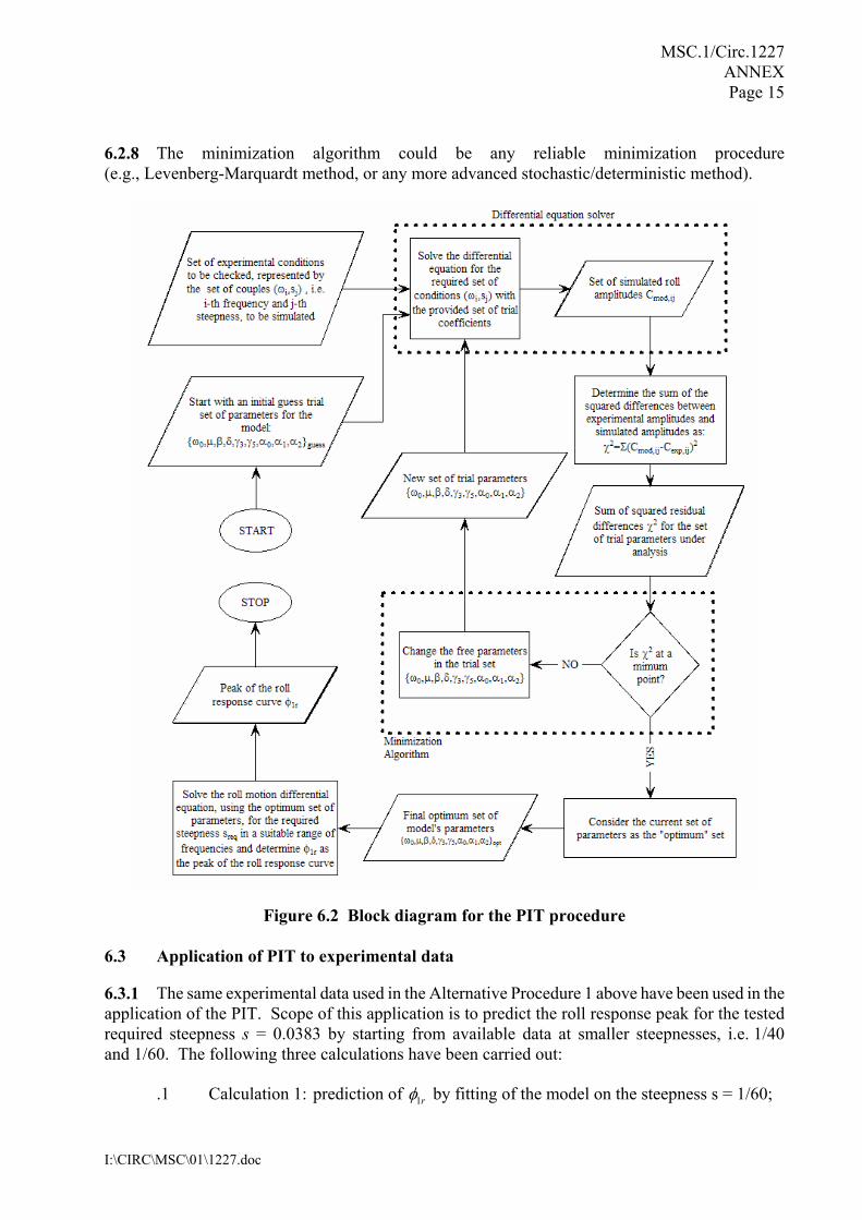
with a cubic term 3δ φ⋅ & could be more suitable for bare hulls. 6.1.13 The use of different nonlinear damping models, can lead to different results in the prediction of the final rolling amplitude. For this reason, in the absence of sufficient evidence for the selection of one nonlinear model versus the others, the use of the average of the two predicted peak rolling amplitudes is recommended. A pure linear model, on the other hand, is almost always inadequate for the representation of roll damping at zero speed. 6.2 General comments on PIT implementation 6.2.1 The PIT technique needs to be implemented in a suitable computer code, and it is not amenable to hand calculations. A block diagram for the implementation of the PIT is reported in figure 6.2. As it can be seen, the procedure is based on two main components:

.1 a differential equation solver used to determine the roll response predicted by the model for different trial sets of parameters; and

.2 a suitable minimization algorithm used to achieve the optimum set of parameters by

minimizing the sum of the squared differences between experimental and predicted roll amplitudes.

6.2.2 The differential equation solver could be basically of two types:

.1 Exact time domain solver: it numerically solves the general differential equation (N-6.1) by using discrete time step algorithms (like the Runge-Kutta) for a certain number of forcing periods, until the roll steady state is achieved. Finally, each time history is analysed in order to get the steady state roll amplitude; and



.2 Approximate frequency domain solver: it uses an analytical approximate solution of

the differential equation (N-6.1) in order to determine the nonlinear roll response curve in frequency domain. Typically used analytical methods are the harmonic balance technique, the multiple scale method and the averaging technique [3].

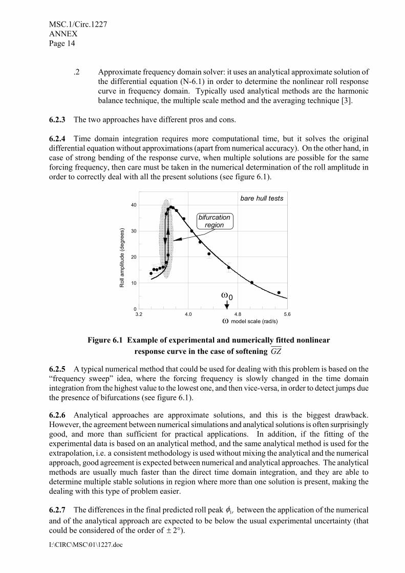
6.2.3 The two approaches have different pros and cons. 6.2.4 Time domain integration requires more computational time, but it solves the original differential equation without approximations (apart from numerical accuracy). On the other hand, in case of strong bending of the response curve, when multiple solutions are possible for the same forcing frequency, then care must be taken in the numerical determination of the roll amplitude in order to correctly deal with all the present solutions (see figure 6.1).

3.2 4.0 4.8 5.6ω model scale (rad/s)

0

10

20

30

40bare hull tests

bifurcationregion

ω0

Figure 6.1 Example of experimental and numerically fitted nonlinear response curve in the case of softening GZ

6.2.5 A typical numerical method that could be used for dealing with this problem is based on the “frequency sweep” idea, where the forcing frequency is slowly changed in the time domain integration from the highest value to the lowest one, and then vice-versa, in order to detect jumps due the presence of bifurcations (see figure 6.1). 6.2.6 Analytical approaches are approximate solutions, and this is the biggest drawback. However, the agreement between numerical simulations and analytical solutions is often surprisingly good, and more than sufficient for practical applications. In addition, if the fitting of the experimental data is based on an analytical method, and the same analytical method is used for the extrapolation, i.e. a consistent methodology is used without mixing the analytical and the numerical approach, good agreement is expected between numerical and analytical approaches. The analytical methods are usually much faster than the direct time domain integration, and they are able to determine multiple stable solutions in region where more than one solution is present, making the dealing with this type of problem easier. 6.2.7 The differences in the final predicted roll peak 1rφ between the application of the numerical and of the analytical approach are expected to be below the usual experimental uncertainty (that could be considered of the order of ± 2°).

Rol

l am

plitu

de (d

egre

es)



6.2.8 The minimization algorithm could be any reliable minimization procedure (e.g., Levenberg-Marquardt method, or any more advanced stochastic/deterministic method).

Figure 6.2 Block diagram for the PIT procedure 6.3 Application of PIT to experimental data 6.3.1 The same experimental data used in the Alternative Procedure 1 above have been used in the application of the PIT. Scope of this application is to predict the roll response peak for the tested required steepness s = 0.0383 by starting from available data at smaller steepnesses, i.e. 1/40 and 1/60. The following three calculations have been carried out:

.1 Calculation 1: prediction of 1rφ by fitting of the model on the steepness s = 1/60;



.2 Calculation 2: prediction of 1rφ by fitting of the model on the steepness s = 1/40; .3 Calculation 3: prediction of 1rφ by fitting of the model on both the steepness

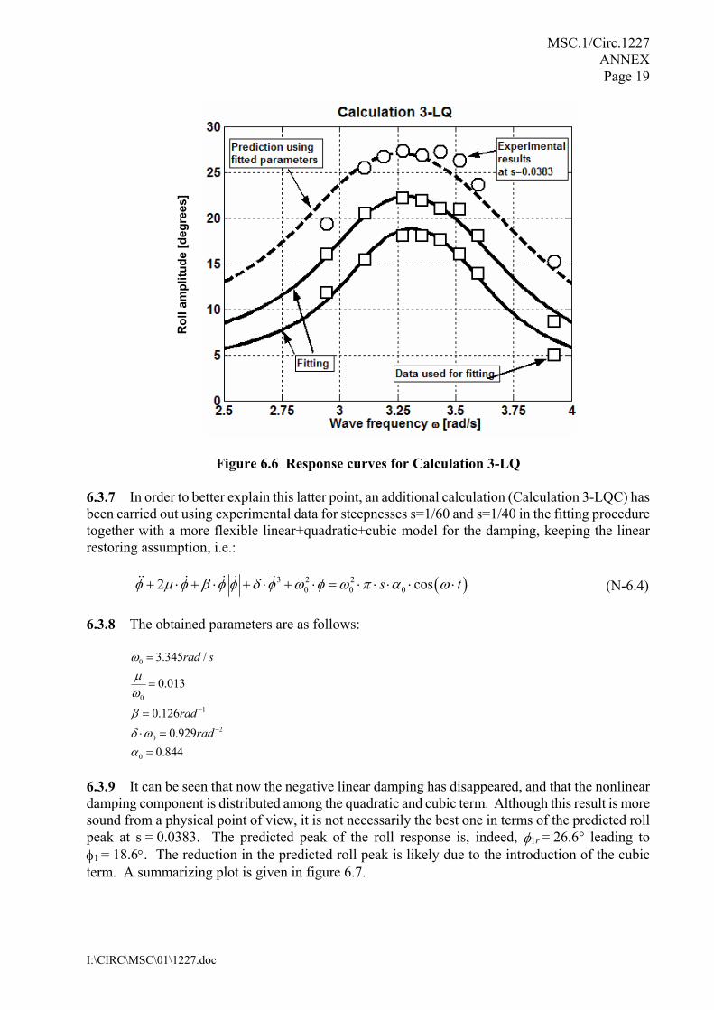
s = 1/40 and s = 1/60; 6.3.2 In the case of calculations 1 and 2, being only one steepness available, the reduced model (N-6.2) has been used, and because of the linearity of the GZ curve and because of the absence of any evident bending in the response curve it has been assumed that 3 0γ = . 6.3.3 In the case of calculation 3, being two steepnesses available, additional terms have been added. Two different analytical model have then been used: the first model is exactly the same as that used for calculation 1 and 2, whereas in the second model the linear damping coefficient µ has been left free (see (N-6.3)). However, in both cases, the assumption of linear restoring, i.e., 3 0γ = and 5 0γ = , has been kept. 6.3.4 In all cases the roll response curve has been determined through an analytical approximate nonlinear frequency domain approach where the response curve is obtained by means of the harmonic balance technique [3]. 6.3.5 The used analytical models and the results obtained through the application of the PIT are summarized in Table 6.1, while a global picture of the roll response curves is given from figure 6.3 to figure 6.6. 6.3.6 From the analysis of the reported exercise it seems that the PIT together with the proposed analytical reduced models is able to reasonably predict the ship roll response curve at the largest steepness by starting from the fitting of the roll response curve(s) experimentally obtained at lower steepnesses. The pure quadratic damping model allows for the achievement of good predictions of the experimental peak, probably thanks to the presence of bilge keels. In the case of linear+quadratic damping model, a negative linear damping coefficient has been obtained, that is, of course, physically meaningless. However, the equivalent linear damping in the range of tested angles as given by the fitted model in Calculation 3-LQ is, of course, positive. The negative sign in the linear damping coefficient is thus due to the fact that the equivalent linear damping obtained from the fitted model in the range of tested rolling amplitudes better fits the experimental data according to the minimization procedure. If a series of experiments had been carried out at smaller steepnesses with subsequent fitting, it would have increased the linear damping coefficient, making it, probably, positive. Bearing in mind the theoretical background of the PIT technique, negative linear damping coefficients are often not a real practical problem, even if their presence usually indicates that different types of analytical modelling for the damping function could lead to a better representation of the real ship damping.



Table 6.1 Analytical models used in the fitting and fitted parameters (model scale)

Calculation 1 Calculation 2 Calculation 3-Q Calculation 3-LQ Steepness used

in the fitting 1/60 1/40 1/60 and 1/40

Analytical model ( )ts ⋅⋅⋅⋅⋅

=⋅+⋅⋅+

ωαπω

φωφφβφ

cos020

20&&&&

( )

20

20 0

2

coss t

φ µ φ β φ φ ω φ

ω π α ω

+ ⋅ + ⋅ + ⋅ =

= ⋅ ⋅ ⋅ ⋅ ⋅

&& & & &

Fitted coefficients

0

1

0

3.344 /

0.520

0.873

rad s

rad

ω

β

α

−

=

=

=

0

1

0

3.348 /

0.518

0.857

rad s

rad

ω

β

α

−

=

=

=

0

1

0

3.346 /

0.519

0.864

rad s

rad

ω

β

α

−

=

=

=

0

0

1

0

3.345 /

0.028

0.684

0.833

rad s

rad

ω

µ

ω

β

α

−

=

= −

=

=

Predicted value in degrees of

1rφ for

0383.0=s

28.3 28.1 28.2 27.0

Corresponding value of

1 10.7 rφ φ= ⋅ 19.8 19.7 19.7 18.9

Experimentally determined 1φ

in degrees 19.3

Figure 6.3 Response curves for Calculation 1

Rol

l am

plitu

de [d

egre

es]



Figure 6.4 Response curves for Calculation 2

Figure 6.5 Response curves for Calculation 3-Q

Rol

l am

plitu

de [d

egre

es]

Rol

l am

plitu

de [d

egre

es]



Figure 6.6 Response curves for Calculation 3-LQ 6.3.7 In order to better explain this latter point, an additional calculation (Calculation 3-LQC) has been carried out using experimental data for steepnesses s=1/60 and s=1/40 in the fitting procedure together with a more flexible linear+quadratic+cubic model for the damping, keeping the linear restoring assumption, i.e.:

( )3 2 20 0 02 coss tφ µ φ β φ φ δ φ ω φ ω π α ω+ ⋅ + ⋅ + ⋅ + ⋅ = ⋅ ⋅ ⋅ ⋅ ⋅&& & & & & (N-6.4)

6.3.8 The obtained parameters are as follows:

0

01

20

0

3.345 /

0.013

0.1260.929

0.844

rad s

radrad

ωµ

ω

β

δ ωα

−

−

=

=

=

⋅ =

=

6.3.9 It can be seen that now the negative linear damping has disappeared, and that the nonlinear damping component is distributed among the quadratic and cubic term. Although this result is more sound from a physical point of view, it is not necessarily the best one in terms of the predicted roll peak at s = 0.0383. The predicted peak of the roll response is, indeed, φ1r = 26.6° leading to φ1 = 18.6°. The reduction in the predicted roll peak is likely due to the introduction of the cubic term. A summarizing plot is given in figure 6.7.

Rol

l am

plitu

de [d

egre

es]



Figure 6.7 Response curves for Calculation 3-LQC 6.4 Final remarks 6.4.1 The PIT technique has successfully been applied to the experimental data used in the previous sections for the application of the Three Steps Procedure. 6.4.2 It can be concluded that, for the ship under analysis, a pure quadratic model for damping, together with a pure linear model for the restoring term is sufficient, for practical purposes, to predict the roll peak 1rφ at the steepness required by the alternative assessment of Weather Criterion. 6.4.3 It is however important to underline that for ships having significant nonlinear GZ curves, it is necessary to introduce a nonlinear correction in the restoring term in order to account for the bending of the response curve and the corresponding peak frequency shift. It is in addition noted, from the experience gained from this exercise, that an additional test in the range of low forcing frequencies (say 00.75ω ω= ⋅ ) could help in the fitting of the effective wave slope, allowing to take into account a frequency dependence of this coefficient. This latter frequency dependence could be important when the bending of the response curve is significant. 6.4.4 As an additional note, it can be said that the application of different tentative models in the PIT allows for an assessment of the likely level of uncertainty inherent in the extrapolation. 6.4.5 In the case under analysis, the level of uncertainty is of the order of ± 2°, however this figure strongly depends on the actual analysed case.

Rol

l am

plitu

de [d

egre

es]



6.4.6 The value of the effective wave slope obtained through the PIT (about 0.85 on average) is slightly different from the value obtained through the application of the Three steps procedure (r = 0.759). This difference can be readily explained by recalling that, in the Three steps procedure, the damping is evaluated from the roll decays tests, while the effective wave slope is evaluated from the roll tests in beam waves, using the previously obtained damping coefficient. In the PIT approach, on the contrary, both the damping and the effective wave slope are determined from the same experimental data in beam waves, for this reason the final outcomes could differ in terms of single components. The final predictions of the angle 1rφ given by the PIT technique and by the Three steps procedure are however very close: the two alternative procedures can be then considered, for this particular case, as equivalent from a practical point of view. 6.5 References [1] Francescutto, A., Contento, G., “Bifurcations in Ship Rolling: Experimental Results and

Parameter Identification Technique”, Ocean Engineering, Vol. 26, 1999, pp. 1095-1123. [2] Tzamtzis, S., Francescutto, A., Bulian, G. and Spyrou, K., “Development and testing of a

procedure for the alternative assessment of Weather Criterion on experimental basis”, Technical Report, University of Trieste, Dept. Naval Architecture & Environmental Engineering, 2005.

[3] Nayfeh, A.H., Mook, D.T., “Nonlinear Oscillations”, John Wiley & Sons, Inc., 1979. [4] IMO Document, SLF 47/6/18, “Proposal of Guidelines for a standard model test procedure to

determine the steady wind heeling lever”, Submitted by Italy and Japan, 7 July 2004. [5] IMO Document, SLF 47/6/19, “Proposal of Guidelines for model tests to determine the roll

angle for the weather criterion”, Submitted by Japan, 7 July 2004. [6] IMO Document, SLF 48/4/15, “Comments on draft guidelines for alternative assessment of

weather criterion based on trial experiment results”, Submitted by Japan, 8 July 2005.

______________

Documents

EXPLANATORY NOTES TO THE INTERIM … Covered by IMO Instruments (resolution A.749(18)). 2 Member Governments are invited to bring the annexed Explanatory Notes to the Interim