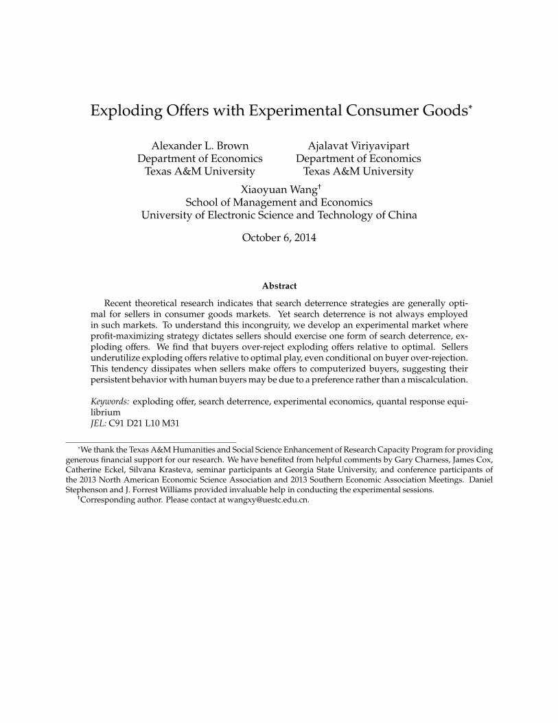
Exploding Offers with Experimental Consumer Goods∗

Alexander L. BrownDepartment of Economics

Texas A&M University

Ajalavat ViriyavipartDepartment of Economics

Texas A&M University

Xiaoyuan Wang†School of Management and Economics

University of Electronic Science and Technology of China

October 6, 2014

Abstract

Recent theoretical research indicates that search deterrence strategies are generally opti-mal for sellers in consumer goods markets. Yet search deterrence is not always employedin such markets. To understand this incongruity, we develop an experimental market whereprofit-maximizing strategy dictates sellers should exercise one form of search deterrence, ex-ploding offers. We find that buyers over-reject exploding offers relative to optimal. Sellersunderutilize exploding offers relative to optimal play, even conditional on buyer over-rejection.This tendency dissipates when sellers make offers to computerized buyers, suggesting theirpersistent behavior with human buyers may be due to a preference rather than a miscalculation.

Keywords: exploding offer, search deterrence, experimental economics, quantal response equi-libriumJEL: C91 D21 L10 M31

∗We thank the Texas A&M Humanities and Social Science Enhancement of Research Capacity Program for providinggenerous financial support for our research. We have benefited from helpful comments by Gary Charness, James Cox,Catherine Eckel, Silvana Krasteva, seminar participants at Georgia State University, and conference participants ofthe 2013 North American Economic Science Association and 2013 Southern Economic Association Meetings. DanielStephenson and J. Forrest Williams provided invaluable help in conducting the experimental sessions.

†Corresponding author. Please contact at wangxy@uestc.edu.cn.

1 Introduction

One of the first applications of microeconomic theory is to the consumer goods market: basic

supply and demand models can often explain transactions in centralized markets quite well.

When markets are decentralized, often additional modeling is required to explain the interactions

of consumers and producers. One popular model, a search model, suggests consumers sample

prices from a variety of producers, buying once the price of goods falls below a certain threshold

(Stigler, 1961; Rothschild, 1974). If decisions of sellers can affect buyer search, the model becomes

more complicated. Armstrong and Zhou (2013) show under relatively mild conditions, it is

unilaterally profitable for sellers to deter search. Specifically the strategies of exploding offers (i.e.,

“take-it-or-leave-it” offers), “buy-now” discounts, and requiring deposits for the option to buy

later are profitable for sellers. Given the profitability of such strategies, a natural question to ask

is why they are not seen more often in market transactions. One possibility is that producers are

justifiably concerned that consumers may respond more negatively to these tactics than theory

predicts. The focus of this paper will be an experimental investigation of this question: whether

producers are hesitant to use exploding offers and whether consumers respond more negatively

to such offers than theory predicts. We choose the tactic of offering exploding offers over the other

two search-deterrence tactics (i.e.,“buy-now” discounts, deposits) because (1) it is an extreme case

of the other two tactics; (2) it is the most simple to understand; and (3) it is the most likely of the

three to generate a negative reaction from buyers.

Prior to Armstrong and Zhou (2013), the focus of most economic research on exploding offers

concerned labor markets, a type of market where there are specific cases of exploding offers

being the norm.1 There may be distinct features of labor markets—not found in consumer goods

markets—that are responsible for the prevalence of exploding offers. Exploding offers may be an

essential tool in the unraveling of matching markets, as employers compete to lock down new

employees earlier and earlier (Niederle and Roth, 2009). Additionally, if employers are required

to have only one outstanding offer to a candidate at a time, exploding offers can be seen as a

technique to “forestall the event that no one is hired” (Lippman and Mamer, 2012). Evidence of

negative responses to exploding offers also relies on features unique to labor markets. Lau et al.

(forthcoming) find experimental evidence that employees will respond negatively to employers’

use of exploding offers by reducing effort after being hired; there is no equivalent reaction that

1For instance, law students applying for appellate court clerkships frequently receive exploding offers (Roth andXing, 1994; Avery et al., 2001, 2007; Niederle and Roth, 2009).

1

could occur in consumer goods markets.

Thus it is an open question how individuals will react to exploding offers in consumer goods

markets, a setting where the use of such offers is notably different from labor markets. Observing

behavior of buyers and sellers in situations with exploding offers would be difficult. Firms do not

have incentives to record or publicly release their use of exploding offers. Moreover, markets may

offer more durable products or long term services, and receive certain amounts of new demand at

each period, which makes information less transparent and traceable at the individual consumer

level.

For these reasons we turn to experimental analysis, the first such analysis of exploding offers

in the consumer goods setting. We implement a simplified version of Armstrong and Zhou (2013):

two sellers simultaneously choose from one of three prices and either make an exploding or

non-exploding offer. Buyers, previously unaware of their personal value for either seller’s good,

randomly visit one seller and learn their value for that seller’s good. In doing so, they receive the

seller’s offer. The buyer must then decide whether to visit the other seller. If the first seller makes

an exploding offer, a visit to the second seller will terminate the opportunity to buy from the first

seller. If our intuition and previous experimental results are any guide, buyers will over-reject

exploding offers. They will choose to visit the second seller more often than theory would predict.

Sellers may also make decisions inconsistent with theory.

We can observe the behavior of buyers directly. Sellers’ behavior, however, is conditional on

perceived buyer response. To isolate this effect, we use two treatments. In one, sellers knowingly

interact with computer buyers programmed to follow optimal strategy; in the other they interact

with human buyers.

Our results are striking. Consistent with our intuition, buyers reject exploding offers roughly

20% more often than optimal theory dictates. The tendency persists through all twenty periods of

the experiment. Sellers make exploding offers less often to human buyers than computer buyers.

Adjusting payoffs for sellers to account for the increased propensity of buyers to reject exploding

offers, we find that sellers still are hesitant to give human buyers exploding offers, a tendency

we term “exploding-offer aversion.” The net result of these differences from optimal strategy is a

transfer of surplus from sellers to buyers. That is, seller payoffs in the computer-buyer treatment

are higher than in the human-buyer treatment, and human buyers earn more than computer

buyers.

These results can help explain why exploding offers in consumer markets may not be as

2

prevalent as theoretically predicted. Buyers will likely reject them more than the optimal level.

Sellers make fewer exploding offers than optimal even after accounting for this buyer behavior.

Although one should be cautious in making field predictions directly from the results of laboratory

data, it is important to note that many of the features that might make sellers hesitant to use

exploding offers and buyers quick to reject them are not present in this laboratory environment.

Sellers make offers anonymously and are somewhat insulated from the negative feelings of having

their offer rejected. Buyers may find exploding offers less objectionable on a computer interface

than through an actual human seller. So there are some reasons to suggest that the tendencies

found in this experiment might be amplified in actual field market situations.

The remainder of the paper is organized as follows: Section 2 provides the theoretical model

used in our experiment. Section 3 discusses our experimental design. Section 4 presents the

results. Section 5 closes the paper with a brief discussion of related work and concluding remarks.

2 The Model

The experiment in this paper implements a simplified model based on Armstrong and Zhou

(2013). The following section describes the basic setup of the model and the assumptions and

simplifications used in the experiment. Section 2.1 explains how the sequential search game takes

place. Sections 2.2 and 2.3 explain the optimization problem for the buyer and seller, respectively.

Section 2.4 describes simplifying assumptions and parameter choices that will be used in the

experiment. The main changes from the literature are to discretize buyer valuations and seller

pricing. This change reduces the number of decisions for subjects, simplifying the problem.

Assuming optimal play by buyers, the end result is a 6 x 6 symmetric normal-form game between

two sellers. Table 1 (at the end of this section) provides payoffs for a seller given a fixed offer and

pricing choice strategy, conditional on the other seller’s pricing and offer choice strategy. The table

will be used as a theoretical benchmark for analysis of sellers choices in the experimental game.

2.1 The Search

This model represents an experimental search market of two sellers with one buyer who vis-

its each seller sequentially in a random order.2 Each seller offers a good which has a pri-

2Several identical buyers were used in our experiments for a larger sample size. Each seller can only choose onestrategy for all buyers in each period.

3

vate value for the buyer drawn from the same ex-ante value distribution: Vik ∈

{Vi

1,Vi2, ...,V

iK

}(where i = 1, 2 represents sellers and k = 1, 2, ...,K represents K possible values) with probability

υ1 ≡ prob(V1), υ2 ≡ prob(V2), ..., υK ≡ p(VK). The game is as follows:

1. Each seller sets a price from a possible price range: Pi∈

{Pi

1,Pi2, ...,P

iL

}and chooses an offer

type as either an exploding or a free-recall offer.

2. Nature randomly selects which seller the buyer will visit first (S1).3

3. The buyer observes the prices of both sellers (P1 and P2) and his value of the first good he4

visits (V1).

4. The buyer chooses whether to accept the first offer or to visit S2. If he chooses to accept, the

transaction occurs and the game is ended; otherwise, the game continues to the next step.

5. The buyer visits S2 and observes the value of the good (V2).

6. The buyer chooses whether to accept or reject the offer from S2. If he accepts, the transaction

occurs and the game is ended. If he rejects and the first offer was an exploding offer, no

transaction occurs and the game is ended. If he rejects and the first offer was a free-recall

offer, the game continues to the next step.

7. The buyer chooses whether to accept or reject the offer from S1 (if it is a free-recall offer).

Each player’s payoff is determined after the game is ended. If there are no transactions, all players

receive zero payoff. If there is a transaction, the buyer receives a payoff equal to the difference

between his value and the price of the good he bought; that seller receives a payoff equals to that

price; the (other) seller with no transaction receives zero payoff.

2.2 Buyer Best Response

We assume that the buyer is rational and has an objective to maximize his expected payoff. Because

the offer type of the second seller has no effect on a strategy of the buyer, we only need to consider

two cases; (1) the first offer is a free-recall offer and (2) the first offer is an exploding offer.

3We denote the first seller S1 and the other seller S2.4As a convention, we assume female sellers and a male buyer.

4

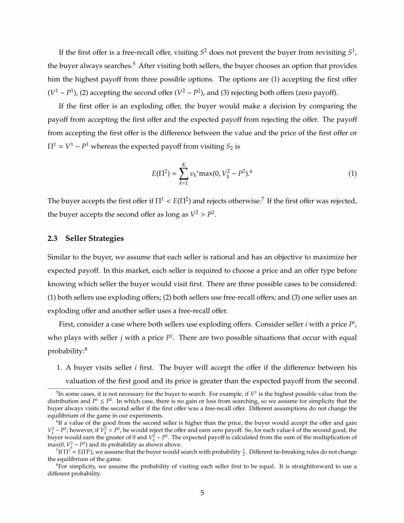
If the first offer is a free-recall offer, visiting S2 does not prevent the buyer from revisiting S1,

the buyer always searches.5 After visiting both sellers, the buyer chooses an option that provides

him the highest payoff from three possible options. The options are (1) accepting the first offer

(V1− P1), (2) accepting the second offer (V2

− P2), and (3) rejecting both offers (zero payoff).

If the first offer is an exploding offer, the buyer would make a decision by comparing the

payoff from accepting the first offer and the expected payoff from rejecting the offer. The payoff

from accepting the first offer is the difference between the value and the price of the first offer or

Π1 = V1− P1 whereas the expected payoff from visiting S2 is

E(Π2) =

K∑k=1

υk∗max(0,V2

k − P2).6 (1)

The buyer accepts the first offer if Π1 < E(Π2) and rejects otherwise.7 If the first offer was rejected,

the buyer accepts the second offer as long as V2 > P2.

2.3 Seller Strategies

Similar to the buyer, we assume that each seller is rational and has an objective to maximize her

expected payoff. In this market, each seller is required to choose a price and an offer type before

knowing which seller the buyer would visit first. There are three possible cases to be considered:

(1) both sellers use exploding offers; (2) both sellers use free-recall offers; and (3) one seller uses an

exploding offer and another seller uses a free-recall offer.

First, consider a case where both sellers use exploding offers. Consider seller i with a price Pi,

who plays with seller j with a price P j. There are two possible situations that occur with equal

probability:8

1. A buyer visits seller i first. The buyer will accept the offer if the difference between his

valuation of the first good and its price is greater than the expected payoff from the second5In some cases, it is not necessary for the buyer to search. For example, if V1 is the highest possible value from the

distribution and P1≤ P2. In which case, there is no gain or loss from searching, so we assume for simplicity that the

buyer always visits the second seller if the first offer was a free-recall offer. Different assumptions do not change theequilibrium of the game in our experiments.

6If a value of the good from the second seller is higher than the price, the buyer would accept the offer and gainV2

k − P2; however, if V2k < P2, he would reject the offer and earn zero payoff. So, for each value k of the second good, the

buyer would earn the greater of 0 and V2k − P2. The expected payoff is calculated from the sum of the multiplication of

max(0,V2k − P2) and its probability as shown above.

7If Π1 = E(Π2), we assume that the buyer would search with probability 12 . Different tie-breaking rules do not change

the equilibrium of the game.8For simplicity, we assume the probability of visiting each seller first to be equal. It is straightforward to use a

different probability.

5

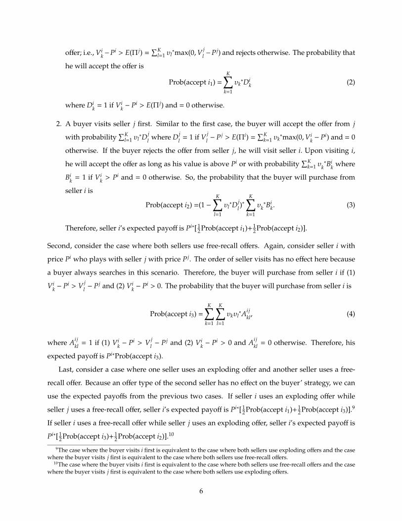
offer; i.e., Vik−Pi > E(Π j) =

∑Kl=1 υl

∗max(0,V jl −P j) and rejects otherwise. The probability that

he will accept the offer is

Prob(accept i1) =

K∑k=1

υk∗Di

k (2)

where Dik = 1 if Vi

k − Pi > E(Π j) and = 0 otherwise.

2. A buyer visits seller j first. Similar to the first case, the buyer will accept the offer from j

with probability∑K

l=1 υl∗D j

l where D jl = 1 if V j

l − P j > E(Πi) =∑K

k=1 υk∗max(0,Vi

k − Pi) and = 0

otherwise. If the buyer rejects the offer from seller j, he will visit seller i. Upon visiting i,

he will accept the offer as long as his value is above Pi or with probability∑K

k=1 υk∗Bi

k where

Bik = 1 if Vi

k > Pi and = 0 otherwise. So, the probability that the buyer will purchase from

seller i is

Prob(accept i2) =(1 −K∑

l=1

υl∗D j

l )∗

K∑k=1

υk∗Bi

k. (3)

Therefore, seller i’s expected payoff is Pi∗[ 12 Prob(accept i1)+ 1

2 Prob(accept i2)].

Second, consider the case where both sellers use free-recall offers. Again, consider seller i with

price Pi who plays with seller j with price P j. The order of seller visits has no effect here because

a buyer always searches in this scenario. Therefore, the buyer will purchase from seller i if (1)

Vik − Pi > V j

l − P j and (2) Vik − Pi > 0. The probability that the buyer will purchase from seller i is

Prob(accept i3) =

K∑k=1

K∑l=1

υkυl∗Ai j

kl, (4)

where Ai jkl = 1 if (1) Vi

k − Pi > V jl − P j and (2) Vi

k − Pi > 0 and Ai jkl = 0 otherwise. Therefore, his

expected payoff is Pi∗Prob(accept i3).

Last, consider a case where one seller uses an exploding offer and another seller uses a free-

recall offer. Because an offer type of the second seller has no effect on the buyer’ strategy, we can

use the expected payoffs from the previous two cases. If seller i uses an exploding offer while

seller j uses a free-recall offer, seller i’s expected payoff is Pi∗[ 12 Prob(accept i1)+ 1

2 Prob(accept i3)].9

If seller i uses a free-recall offer while seller j uses an exploding offer, seller i’s expected payoff is

Pi∗[ 12 Prob(accept i3)+1

2 Prob(accept i2)].10

9The case where the buyer visits i first is equivalent to the case where both sellers use exploding offers and the casewhere the buyer visits j first is equivalent to the case where both sellers use free-recall offers.

10The case where the buyer visits i first is equivalent to the case where both sellers use free-recall offers and the casewhere the buyer visits j first is equivalent to the case where both sellers use exploding offers.

6

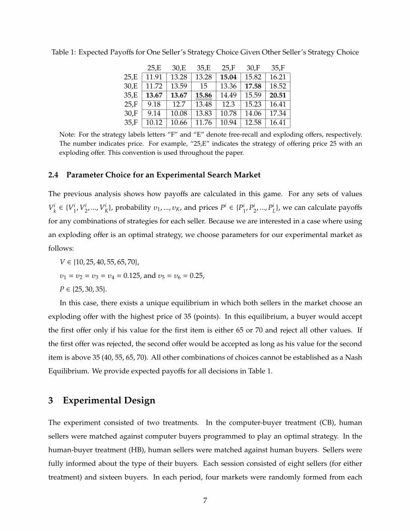
Table 1: Expected Payoffs for One Seller’s Strategy Choice Given Other Seller’s Strategy Choice

25,E 30,E 35,E 25,F 30,F 35,F25,E 11.91 13.28 13.28 15.04 15.82 16.2130,E 11.72 13.59 15 13.36 17.58 18.5235,E 13.67 13.67 15.86 14.49 15.59 20.5125,F 9.18 12.7 13.48 12.3 15.23 16.4130,F 9.14 10.08 13.83 10.78 14.06 17.3435,F 10.12 10.66 11.76 10.94 12.58 16.41

Note: For the strategy labels letters “F” and “E” denote free-recall and exploding offers, respectively.The number indicates price. For example, “25,E” indicates the strategy of offering price 25 with anexploding offer. This convention is used throughout the paper.

2.4 Parameter Choice for an Experimental Search Market

The previous analysis shows how payoffs are calculated in this game. For any sets of values

Vik ∈ {V

i1,V

i2, ...,V

iK}, probability υ1, ..., υK, and prices Pi

∈ {Pi1,P

i2, ...,P

iL}, we can calculate payoffs

for any combinations of strategies for each seller. Because we are interested in a case where using

an exploding offer is an optimal strategy, we choose parameters for our experimental market as

follows:

V ∈ {10, 25, 40, 55, 65, 70},

υ1 = υ2 = υ3 = υ4 = 0.125, and υ5 = υ6 = 0.25,

P ∈ {25, 30, 35}.

In this case, there exists a unique equilibrium in which both sellers in the market choose an

exploding offer with the highest price of 35 (points). In this equilibrium, a buyer would accept

the first offer only if his value for the first item is either 65 or 70 and reject all other values. If

the first offer was rejected, the second offer would be accepted as long as his value for the second

item is above 35 (40, 55, 65, 70). All other combinations of choices cannot be established as a Nash

Equilibrium. We provide expected payoffs for all decisions in Table 1.

3 Experimental Design

The experiment consisted of two treatments. In the computer-buyer treatment (CB), human

sellers were matched against computer buyers programmed to play an optimal strategy. In the

human-buyer treatment (HB), human sellers were matched against human buyers. Sellers were

fully informed about the type of their buyers. Each session consisted of eight sellers (for either

treatment) and sixteen buyers. In each period, four markets were randomly formed from each

7

randomly selected pair of sellers. The market consisted of two sellers and four buyers. In the

every market, two of the buyers visited one seller first and the other two visited the other seller

first.

There were twenty total periods. Each period, buyers and sellers were randomly rematched

into new markets, but the role of each subject (i.e., buyer or seller) was fixed for the entire session.

In addition, the same random matching was used in every session and treatment.11

Each period began with sellers choosing a price and offer type (i.e., exploding or free-recall

offer). The seller’s price and offer types were the same for all buyers that encountered the seller.

Buyers would observe the prices set by both sellers in the market and their offer type, but would

only see their valuation of items from the first seller they encountered. Each buyer’s valuation for

each of the six buying decisions was drawn independently from the known valuation distribution.

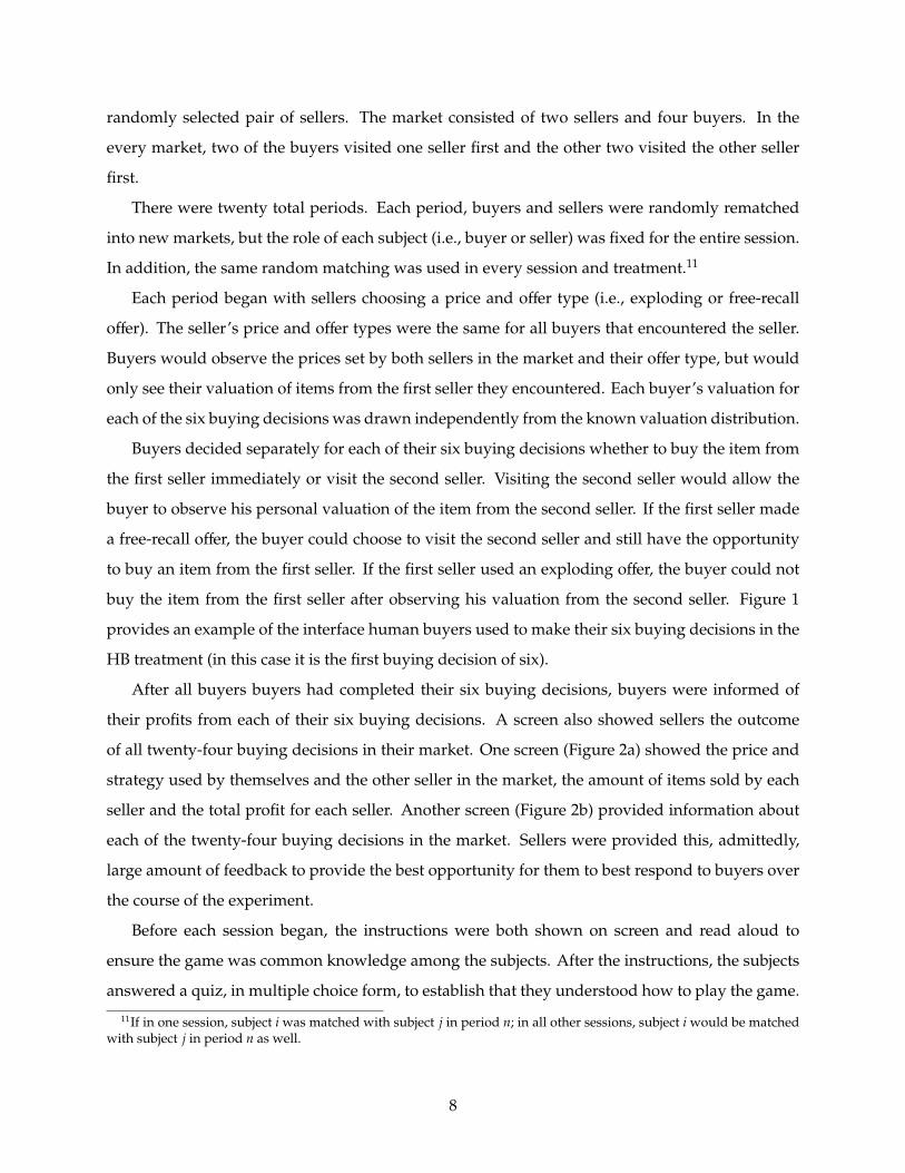
Buyers decided separately for each of their six buying decisions whether to buy the item from

the first seller immediately or visit the second seller. Visiting the second seller would allow the

buyer to observe his personal valuation of the item from the second seller. If the first seller made

a free-recall offer, the buyer could choose to visit the second seller and still have the opportunity

to buy an item from the first seller. If the first seller used an exploding offer, the buyer could not

buy the item from the first seller after observing his valuation from the second seller. Figure 1

provides an example of the interface human buyers used to make their six buying decisions in the

HB treatment (in this case it is the first buying decision of six).

After all buyers buyers had completed their six buying decisions, buyers were informed of

their profits from each of their six buying decisions. A screen also showed sellers the outcome

of all twenty-four buying decisions in their market. One screen (Figure 2a) showed the price and

strategy used by themselves and the other seller in the market, the amount of items sold by each

seller and the total profit for each seller. Another screen (Figure 2b) provided information about

each of the twenty-four buying decisions in the market. Sellers were provided this, admittedly,

large amount of feedback to provide the best opportunity for them to best respond to buyers over

the course of the experiment.

Before each session began, the instructions were both shown on screen and read aloud to

ensure the game was common knowledge among the subjects. After the instructions, the subjects

answered a quiz, in multiple choice form, to establish that they understood how to play the game.

11If in one session, subject i was matched with subject j in period n; in all other sessions, subject i would be matchedwith subject j in period n as well.

8

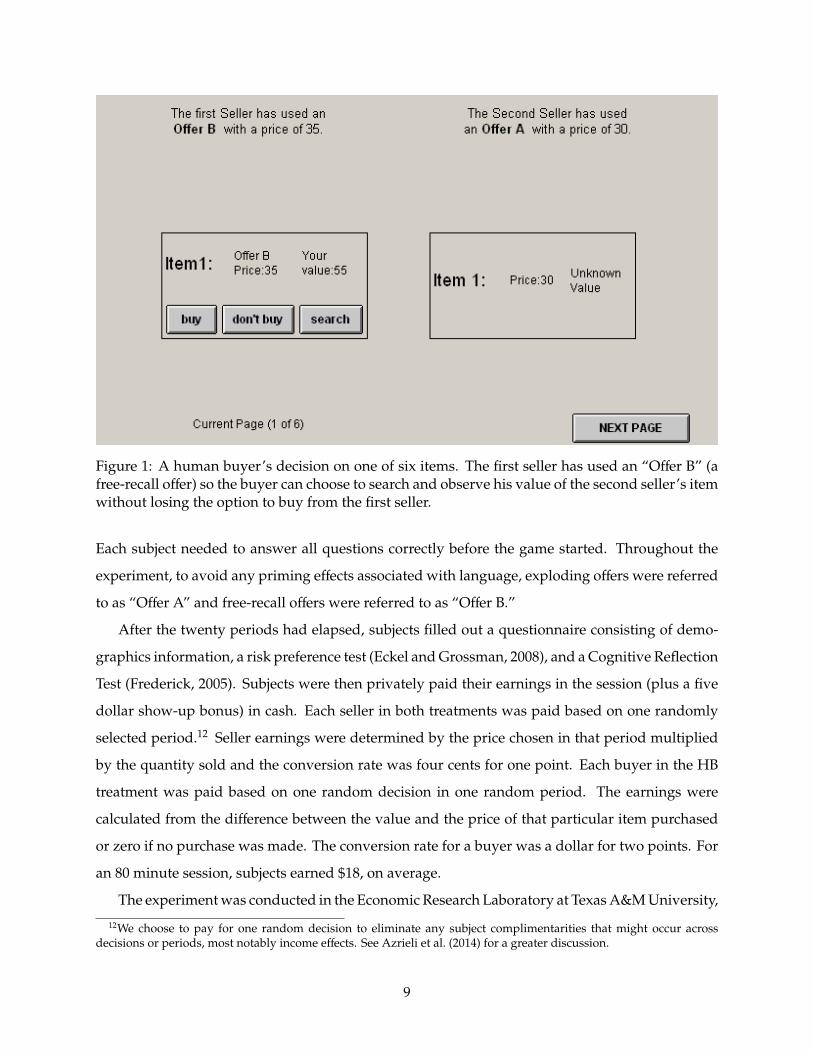
Figure 1: A human buyer’s decision on one of six items. The first seller has used an “Offer B” (afree-recall offer) so the buyer can choose to search and observe his value of the second seller’s itemwithout losing the option to buy from the first seller.

Each subject needed to answer all questions correctly before the game started. Throughout the

experiment, to avoid any priming effects associated with language, exploding offers were referred

to as “Offer A” and free-recall offers were referred to as “Offer B.”

After the twenty periods had elapsed, subjects filled out a questionnaire consisting of demo-

graphics information, a risk preference test (Eckel and Grossman, 2008), and a Cognitive Reflection

Test (Frederick, 2005). Subjects were then privately paid their earnings in the session (plus a five

dollar show-up bonus) in cash. Each seller in both treatments was paid based on one randomly

selected period.12 Seller earnings were determined by the price chosen in that period multiplied

by the quantity sold and the conversion rate was four cents for one point. Each buyer in the HB

treatment was paid based on one random decision in one random period. The earnings were

calculated from the difference between the value and the price of that particular item purchased

or zero if no purchase was made. The conversion rate for a buyer was a dollar for two points. For

an 80 minute session, subjects earned $18, on average.

The experiment was conducted in the Economic Research Laboratory at Texas A&M University,

12We choose to pay for one random decision to eliminate any subject complimentarities that might occur acrossdecisions or periods, most notably income effects. See Azrieli et al. (2014) for a greater discussion.

9

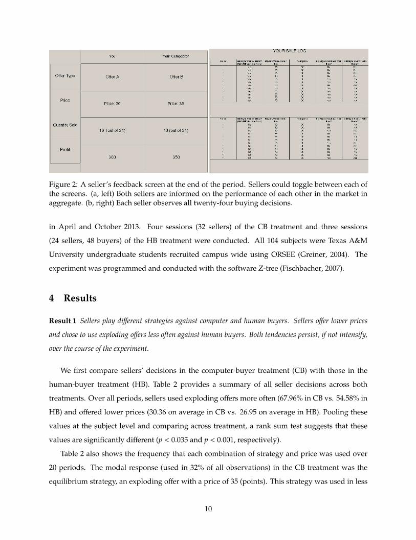
Figure 2: A seller’s feedback screen at the end of the period. Sellers could toggle between each ofthe screens. (a, left) Both sellers are informed on the performance of each other in the market inaggregate. (b, right) Each seller observes all twenty-four buying decisions.

in April and October 2013. Four sessions (32 sellers) of the CB treatment and three sessions

(24 sellers, 48 buyers) of the HB treatment were conducted. All 104 subjects were Texas A&M

University undergraduate students recruited campus wide using ORSEE (Greiner, 2004). The

experiment was programmed and conducted with the software Z-tree (Fischbacher, 2007).

4 Results

Result 1 Sellers play different strategies against computer and human buyers. Sellers offer lower prices

and chose to use exploding offers less often against human buyers. Both tendencies persist, if not intensify,

over the course of the experiment.

We first compare sellers’ decisions in the computer-buyer treatment (CB) with those in the

human-buyer treatment (HB). Table 2 provides a summary of all seller decisions across both

treatments. Over all periods, sellers used exploding offers more often (67.96% in CB vs. 54.58% in

HB) and offered lower prices (30.36 on average in CB vs. 26.95 on average in HB). Pooling these

values at the subject level and comparing across treatment, a rank sum test suggests that these

values are significantly different (p < 0.035 and p < 0.001, respectively).

Table 2 also shows the frequency that each combination of strategy and price was used over

20 periods. The modal response (used in 32% of all observations) in the CB treatment was the

equilibrium strategy, an exploding offer with a price of 35 (points). This strategy was used in less

10

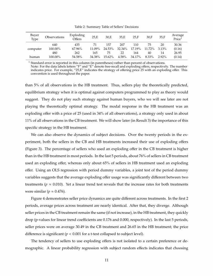
Table 2: Summary Table of Sellers’ Decisions

BuyerType Observations

ExplodingOffers 25,E 30,E 35,E 25,F 30,F 35,F

AveragePrice1

640 435 71 157 207 110 75 20 30.36computer 100.00% 67.96% 11.09% 24.53% 32.34% 17.19% 11.72% 3.13% (0.16)

480 262 165 75 22 164 40 14 26.95human 100.00% 54.58% 34.38% 15.62% 4.58% 34.17% 8.33% 2.92% (0.14)

1 Standard error is reported in this column (in parentheses) rather than percent of observations.Note: For the data labels letters “F” and “E” denote free-recall and exploding offers, respectively. The numberindicates price. For example, “25,E” indicates the strategy of offering price 25 with an exploding offer. Thisconvention is used throughout the paper.

than 5% of all observations in the HB treatment. Thus, sellers play the theoretically predicted,

equilibrium strategy when it is optimal against computers programmed to play as theory would

suggest. They do not play such strategy against human buyers, who we will see later are not

playing the theoretically optimal strategy. The modal response in the HB treatment was an

exploding offer with a price of 25 (used in 34% of all observations), a strategy only used in about

11% of all observations in the CB treatment. We will show later (in Result 3) the importance of this

specific strategy in the HB treatment.

We can also observe the dynamics of subject decisions. Over the twenty periods in the ex-

periment, both the sellers in the CB and HB treatments increased their use of exploding offers

(Figure 3). The percentage of sellers who used an exploding offer in the CB treatment is higher

than in the HB treatment in most periods. In the last 5 periods, about 76% of sellers in CB treatment

used an exploding offer, whereas only about 65% of sellers in HB treatment used an exploding

offer. Using an OLS regression with period dummy variables, a joint test of the period dummy

variables suggests that the average exploding offer usage was significantly different between two

treatments (p ≈ 0.010). Yet a linear trend test reveals that the increase rates for both treatments

were similar (p ≈ 0.476).

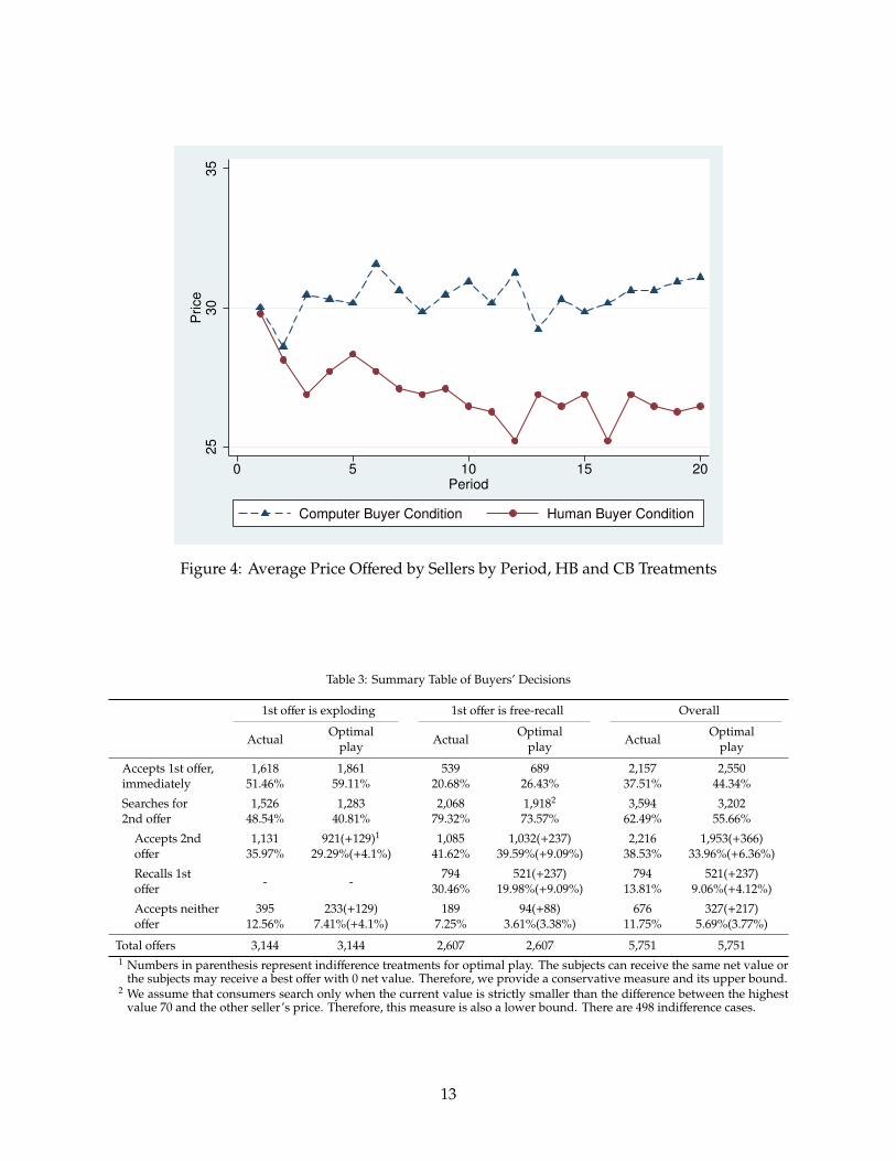
Figure 4 demonstrates seller price dynamics are quite different across treatments. In the first 2

periods, average prices across treatment are nearly identical. After that, they diverge. Although

seller prices in the CB treatment remain the same (if not increase), in the HB treatment, they quickly

drop (p-values for linear trend coefficients are 0.176 and 0.000, respectively). In the last 5 periods,

seller prices were on average 30.49 in the CB treatment and 26.65 in the HB treatment; the price

difference is significant (p < 0.001 for a t-test collapsed to subject level).

The tendency of sellers to use exploding offers is not isolated to a certain preference or de-

mographic. A linear probability regression with subject random effects indicates that choosing

11

0.2

.4.6

.81

Pe

rce

nta

ge

of

exp

lod

ing

off

ers

0 5 10 15 20Period

Computer Buyer Condition Human Buyer Condition

Figure 3: Proportion of Exploding Offers Used by Sellers by Period, HB and CB Treatments

an incrementally safer option on the risk-preference survey, getting an additional CRT question

correct, and being female are all negatively correlated with the tendency to use exploding offers.

However, the correlation is not significant (0.40 < p < 0.76 for all measures).

Result 2 When given an exploding offer, buyers reject the offer (search for the second seller’s item) more

often than profit-maximizing play dictates. This tendency holds over all prices and valuations; it persists

throughout the experiment.

Buyers make 6 purchase attempts in each period over 20 periods. Pooling the results from 3

sessions of 16 buyers each, there are a total of 5,760 (6 × 20 × 16 × 3) purchase attempts. Table

3 provides summary data on all of these choices.13 In 3,144 of these purchase attempts buyers

encounter an exploding offer on the first item they search. Optimal play (based on the price of

the items and buyer valuation of the first item) dictates that buyers should accept this first offer

in 1,861 (59.11%) instances; instead buyers accept in only 1,618 instances (51.46%), a difference

that is statistically significant (p < 0.001 for both a T test and rank sum test at the subject level).14

13Due to a computer glitch 9 buying attempts were unable to be recorded. These affected four different buyers overtwo periods in one session. Given the small number of observations lost compared to the total number in the sample,we cannot envision how this loss of data would affect any results.

14The difference is even more glaring when one considers buyers accepted 49 exploding offers that they should have

12

25

30

35

Price

0 5 10 15 20Period

Computer Buyer Condition Human Buyer Condition

Figure 4: Average Price Offered by Sellers by Period, HB and CB Treatments

Table 3: Summary Table of Buyers’ Decisions

1st offer is exploding 1st offer is free-recall Overall

ActualOptimal

play ActualOptimal

play ActualOptimal

play

Accepts 1st offer,immediately

1,61851.46%

1,86159.11%

53920.68%

68926.43%

2,15737.51%

2,55044.34%

Searches for2nd offer

1,52648.54%

1,28340.81%

2,06879.32%

1,9182

73.57%3,594

62.49%3,202

55.66%

Accepts 2ndoffer

1,13135.97%

921(+129)1

29.29%(+4.1%)1,085

41.62%1,032(+237)

39.59%(+9.09%)2,216

38.53%1,953(+366)

33.96%(+6.36%)

Recalls 1stoffer - -

79430.46%

521(+237)19.98%(+9.09%)

79413.81%

521(+237)9.06%(+4.12%)

Accepts neitheroffer

39512.56%

233(+129)7.41%(+4.1%)

1897.25%

94(+88)3.61%(3.38%)

67611.75%

327(+217)5.69%(3.77%)

Total offers 3,144 3,144 2,607 2,607 5,751 5,7511 Numbers in parenthesis represent indifference treatments for optimal play. The subjects can receive the same net value or

the subjects may receive a best offer with 0 net value. Therefore, we provide a conservative measure and its upper bound.2 We assume that consumers search only when the current value is strictly smaller than the difference between the highest

value 70 and the other seller’s price. Therefore, this measure is also a lower bound. There are 498 indifference cases.

13

The net result is that buyers accept the second offer, the only offer that remains, far more often

than the optimal strategy dictates. Buyers accept the second offer 1,131 (35.97%) times after an

exploding offer, higher than the 921–1,050 (29.29–33.39%) times15 they would if they followed

optimal strategy.

The average expected (net) loss of earnings for such deviation (when a buyer rejects an explod-

ing offer he should accept) is about 7 points per item. If that specific decision was chosen for the

buyer (remember 1 in 120 buying decisions is randomly selected for the buyer), the buyer would

lose $3.50, the equivalent of 7 points. On average buyers made this deviation six times per session

(292 deviations/48 buyers ≈ 6).

It should be noted that buyers also display a tendency to search for a second offer more often

than “optimal” with free-recall offers, though these cases are very different from exploding offers.

In general, buyers with a free-recall offer should continue to search for the second offer unless they

will receive a surplus from the first seller than cannot be beaten by the second seller (e.g., receiving

the highest possible value on an item offered at the lowest possible price). In those cases, it is

unnecessary for buyers to search—the first offer is optimal—but searching produces no economic

loss as buyers may recall their first offer. Buyers with free-recall offers ultimately chose the right

item—the one with the highest net gain—86.74% of the time.16

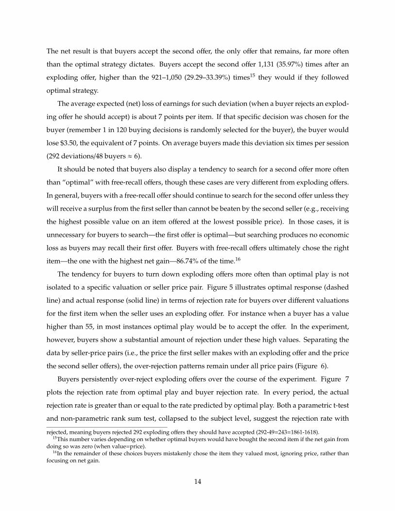
The tendency for buyers to turn down exploding offers more often than optimal play is not

isolated to a specific valuation or seller price pair. Figure 5 illustrates optimal response (dashed

line) and actual response (solid line) in terms of rejection rate for buyers over different valuations

for the first item when the seller uses an exploding offer. For instance when a buyer has a value

higher than 55, in most instances optimal play would be to accept the offer. In the experiment,

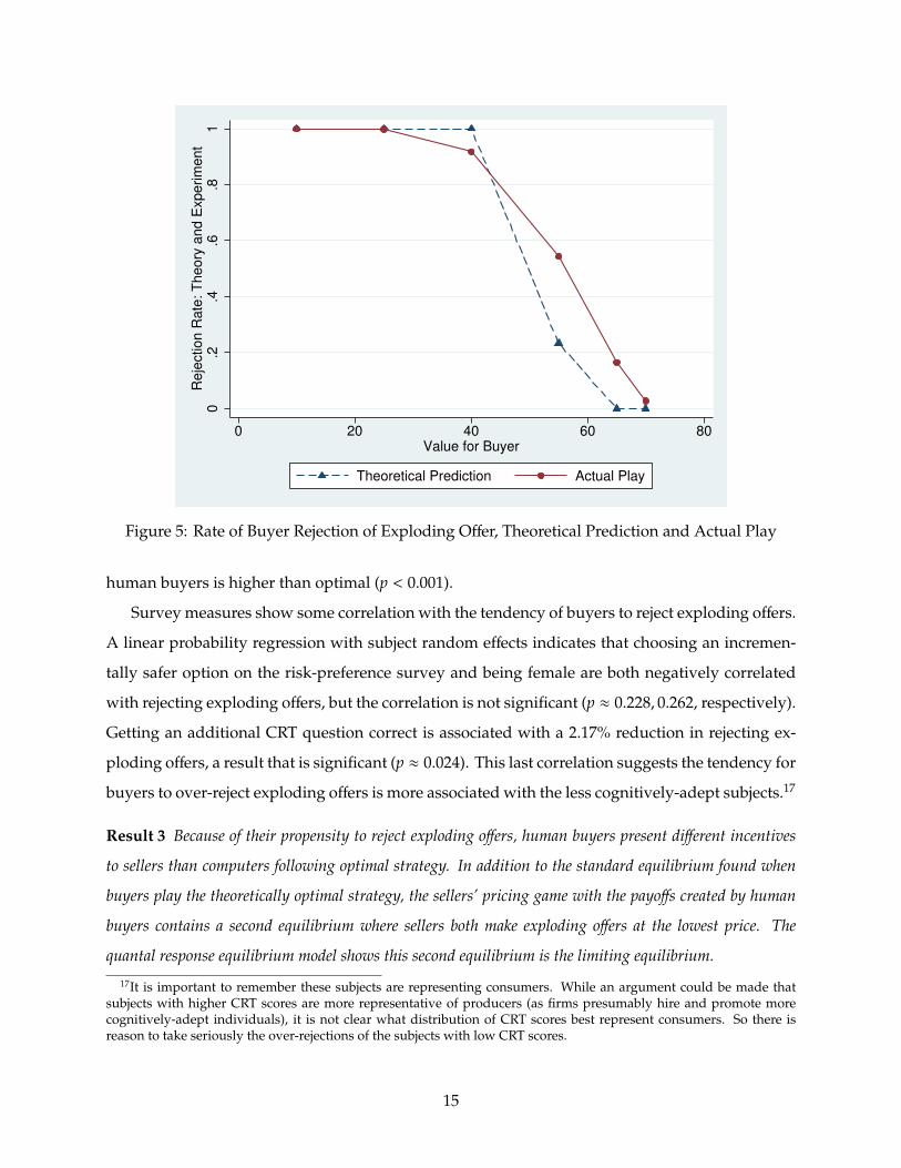
however, buyers show a substantial amount of rejection under these high values. Separating the

data by seller-price pairs (i.e., the price the first seller makes with an exploding offer and the price

the second seller offers), the over-rejection patterns remain under all price pairs (Figure 6).

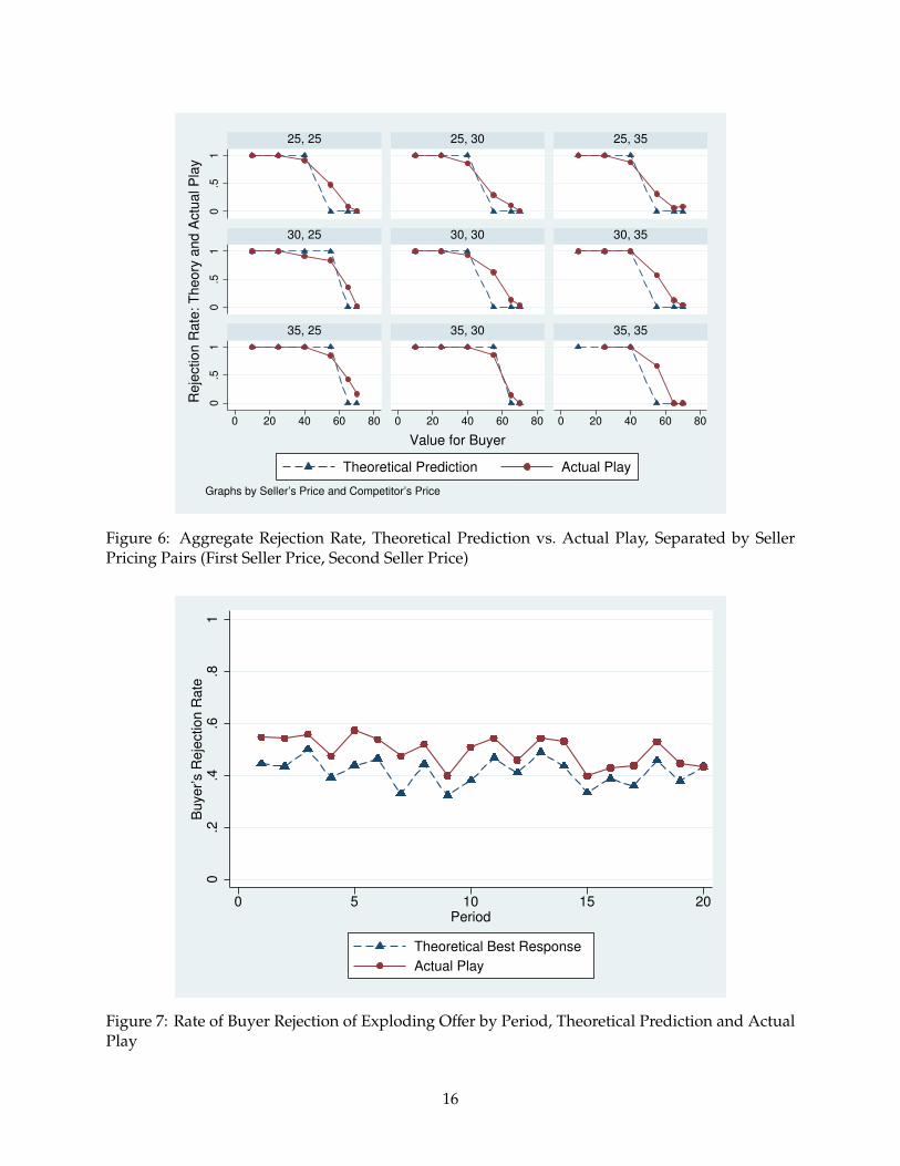
Buyers persistently over-reject exploding offers over the course of the experiment. Figure 7

plots the rejection rate from optimal play and buyer rejection rate. In every period, the actual

rejection rate is greater than or equal to the rate predicted by optimal play. Both a parametric t-test

and non-parametric rank sum test, collapsed to the subject level, suggest the rejection rate with

rejected, meaning buyers rejected 292 exploding offers they should have accepted (292-49=243=1861-1618).15This number varies depending on whether optimal buyers would have bought the second item if the net gain from

doing so was zero (when value=price).16In the remainder of these choices buyers mistakenly chose the item they valued most, ignoring price, rather than

focusing on net gain.

14

0.2

.4.6

.81

Re

jectio

n R

ate

: T

he

ory

an

d E

xp

erim

en

t

0 20 40 60 80Value for Buyer

Theoretical Prediction Actual Play

Figure 5: Rate of Buyer Rejection of Exploding Offer, Theoretical Prediction and Actual Play

human buyers is higher than optimal (p < 0.001).

Survey measures show some correlation with the tendency of buyers to reject exploding offers.

A linear probability regression with subject random effects indicates that choosing an incremen-

tally safer option on the risk-preference survey and being female are both negatively correlated

with rejecting exploding offers, but the correlation is not significant (p ≈ 0.228, 0.262, respectively).

Getting an additional CRT question correct is associated with a 2.17% reduction in rejecting ex-

ploding offers, a result that is significant (p ≈ 0.024). This last correlation suggests the tendency for

buyers to over-reject exploding offers is more associated with the less cognitively-adept subjects.17

Result 3 Because of their propensity to reject exploding offers, human buyers present different incentives

to sellers than computers following optimal strategy. In addition to the standard equilibrium found when

buyers play the theoretically optimal strategy, the sellers’ pricing game with the payoffs created by human

buyers contains a second equilibrium where sellers both make exploding offers at the lowest price. The

quantal response equilibrium model shows this second equilibrium is the limiting equilibrium.

17It is important to remember these subjects are representing consumers. While an argument could be made thatsubjects with higher CRT scores are more representative of producers (as firms presumably hire and promote morecognitively-adept individuals), it is not clear what distribution of CRT scores best represent consumers. So there isreason to take seriously the over-rejections of the subjects with low CRT scores.

15

0.5

10

.51

0.5

1

0 20 40 60 80 0 20 40 60 80 0 20 40 60 80

25, 25 25, 30 25, 35

30, 25 30, 30 30, 35

35, 25 35, 30 35, 35

Theoretical Prediction Actual Play

Re

jectio

n R

ate

: T

he

ory

an

d A

ctu

al P

lay

Value for Buyer

Graphs by Seller’s Price and Competitor’s Price

Figure 6: Aggregate Rejection Rate, Theoretical Prediction vs. Actual Play, Separated by SellerPricing Pairs (First Seller Price, Second Seller Price)

0.2

.4.6

.81

Bu

ye

r’s R

eje

ctio

n R

ate

0 5 10 15 20Period

Theoretical Best Response

Actual Play

Figure 7: Rate of Buyer Rejection of Exploding Offer by Period, Theoretical Prediction and ActualPlay

16

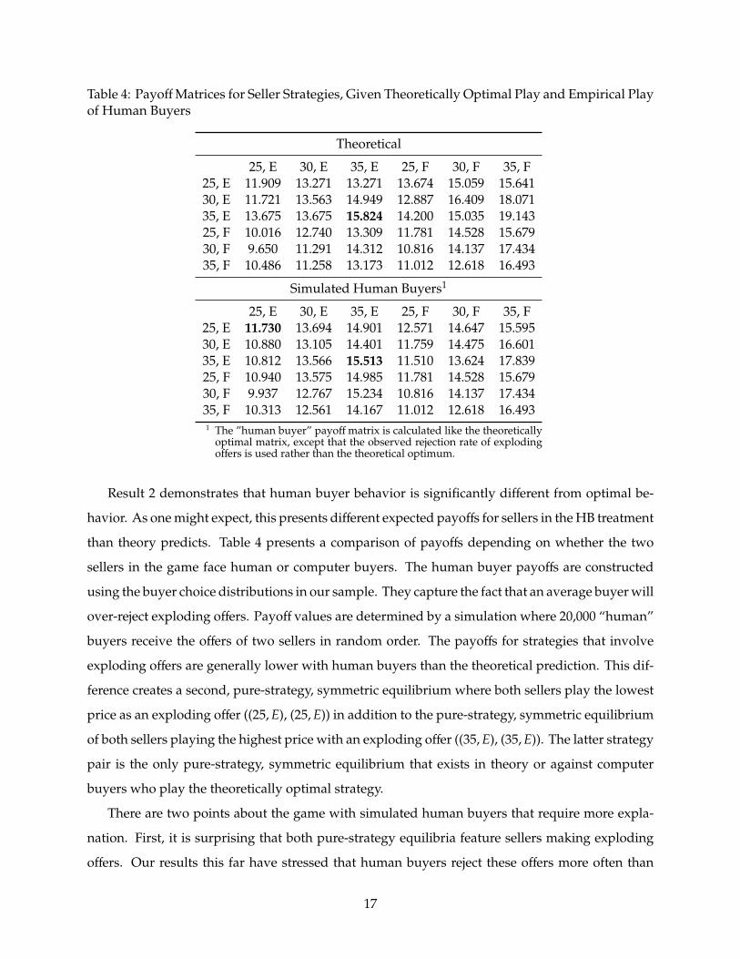
Table 4: Payoff Matrices for Seller Strategies, Given Theoretically Optimal Play and Empirical Playof Human Buyers

Theoretical

25, E 30, E 35, E 25, F 30, F 35, F25, E 11.909 13.271 13.271 13.674 15.059 15.64130, E 11.721 13.563 14.949 12.887 16.409 18.07135, E 13.675 13.675 15.824 14.200 15.035 19.14325, F 10.016 12.740 13.309 11.781 14.528 15.67930, F 9.650 11.291 14.312 10.816 14.137 17.43435, F 10.486 11.258 13.173 11.012 12.618 16.493

Simulated Human Buyers1

25, E 30, E 35, E 25, F 30, F 35, F25, E 11.730 13.694 14.901 12.571 14.647 15.59530, E 10.880 13.105 14.401 11.759 14.475 16.60135, E 10.812 13.566 15.513 11.510 13.624 17.83925, F 10.940 13.575 14.985 11.781 14.528 15.67930, F 9.937 12.767 15.234 10.816 14.137 17.43435, F 10.313 12.561 14.167 11.012 12.618 16.4931 The ”human buyer” payoff matrix is calculated like the theoretically

optimal matrix, except that the observed rejection rate of explodingoffers is used rather than the theoretical optimum.

Result 2 demonstrates that human buyer behavior is significantly different from optimal be-

havior. As one might expect, this presents different expected payoffs for sellers in the HB treatment

than theory predicts. Table 4 presents a comparison of payoffs depending on whether the two

sellers in the game face human or computer buyers. The human buyer payoffs are constructed

using the buyer choice distributions in our sample. They capture the fact that an average buyer will

over-reject exploding offers. Payoff values are determined by a simulation where 20,000 “human”

buyers receive the offers of two sellers in random order. The payoffs for strategies that involve

exploding offers are generally lower with human buyers than the theoretical prediction. This dif-

ference creates a second, pure-strategy, symmetric equilibrium where both sellers play the lowest

price as an exploding offer ((25,E), (25,E)) in addition to the pure-strategy, symmetric equilibrium

of both sellers playing the highest price with an exploding offer ((35,E), (35,E)). The latter strategy

pair is the only pure-strategy, symmetric equilibrium that exists in theory or against computer

buyers who play the theoretically optimal strategy.

There are two points about the game with simulated human buyers that require more expla-

nation. First, it is surprising that both pure-strategy equilibria feature sellers making exploding

offers. Our results this far have stressed that human buyers reject these offers more often than

17

their computer counterparts, seemingly making such strategy less profitable. Making exploding

offers, nonetheless, is still the most profitable of the two seller strategies. Note that if sellers pick

equal prices with different types of offers, the seller with the exploding offer earns higher expected

profits. Lowering prices against an exploding offer can lead to higher payoffs in some cases. Sellers

may find it effective to offer an exploding offer with a lower price to induce a reluctant buyer to

accept an exploding offer.

Second, the existence of two pure-strategy, symmetric equilibria brings up the issue of equilib-

rium selection. It is desirable to be able to focus on one equilibrium and there are many techniques

to do so. We use one such technique, the quantal response equilibrium model (QRE) (McKelvey

and Palfrey, 1995, 1998). The technique will ultimately show that the lower priced equilibrium

((25,E), (25,E)) is the “limiting equilibrium.”

The quantal response equilibrium model (QRE) (McKelvey and Palfrey, 1995, 1998) has become

a standard way to model a game theory data setting where equilibrium strategies are not always

played. For this reason, it is quite often used with experimental data. In a quantal response

equilibrium, each player has correct beliefs about which strategies every other player will play.

Expected payoffs for each strategy choice can be calculated given those beliefs.

πi (si) = E [ui(si, s−i)|si] (5)

Then a given player noisily best responds according to those expected payoffs. Specifically, they

choose strategies with higher expected payoffs more often. As Camerer (2003) notes, typically the

QRE uses a logit payoff response function

P(si) =exp (λπi (si))∑

skexp (λπi (sk)))

. (6)

Because each player calculates P(si) which is dependent on all other players’ values for P(si),

the system is recursive. For a given λ, the solution to the system of equations (6) is a quantal

response equilibrium. The parameter λ measures each player’s sensitivity in responding to these

payoffs. At λ = 0 players play each strategy with equal probability. As λ increases, each player

best responds better, playing higher payoff yielding strategies more frequently, until at λ = ∞

each player is playing a purely best response and we are at a Nash equilibrium, “the limiting

equilibrium.” (McKelvey and Palfrey, 1995)

To model the quantal response equilibrium in our experiment, we use an equivalent formaliza-

18

tion of the QRE model. Rather than having players make noisy choices, we have them maximize

noisy utility functions. The expected utility for a given strategy choice is subject to a random

element. Given consistent beliefs and the strategy set Si, each player i solves the problem

maxsk∈Si

πi (sk) + εik. (7)

The ε’s are independently and identically distributed type-1 extreme value, making the problem

and equilibrium equivalent to the system of equations shown in (6).

Figure 8 illustrates the prevalence of different seller strategies under the quantal response

equilibrium model in the HB and CB treatment. The payoffs given in table 4 are directly used

as sellers’ payoffs for playing different strategies.18 In the CB treatment, exploding offers lead

to consistently better payoffs than free-recall offers given the computer buyers’ optimized play.

In the HB treatment, however, buyers consistently over-reject exploding offers. Modifying seller

payoffs to account for this over-rejection creates a new game, one where both sellers making an

exploding offer with price 25 becomes an additional Nash Equilibrium. Figure 8(b) shows that the

QRE model selects this equilibrium as the limiting equilibrium.

It is interesting to note that this limiting equilibrium strategy is also the modal strategy choice

of sellers in the HB treatment (see Result 1).

Result 4 In both treatments, sellers demonstrate a reluctance to play strategies that involve the use of

exploding offers. The tendency persists through all twenty periods against human buyers, but dissipates

against computer buyers who play optimal strategy. This analysis controls for the differential expected

payoffs of both strategies in the human- and computer-buyer treatments.

The quantal response model provides a baseline utility framework for sellers (see equation 7).

In order to determine whether sellers have any preferences toward exploding offers not captured

in the model, we introduce a new term δ that is included in sellers’ utility only if they make an

exploding offer. If δ is negative (positive), than sellers are reluctant (overeager) to use exploding

offers; they derive additional negative (positive) utility from making them. If δ is zero, sellers do

not have a systematic bias in their use of exploding offers. As the use of exploding offers varies

between treatments and also within treatment by period (see Figure 3), we introduce four terms to

capture the dynamics and treatment effects of exploding offers. The terms δH0, δHT represent the

18To be clear, this means we are analyzing a two-player, normal-form game. We set buyer behavior as fixed. That is,we are not using QRE to model buyer behavior.

19

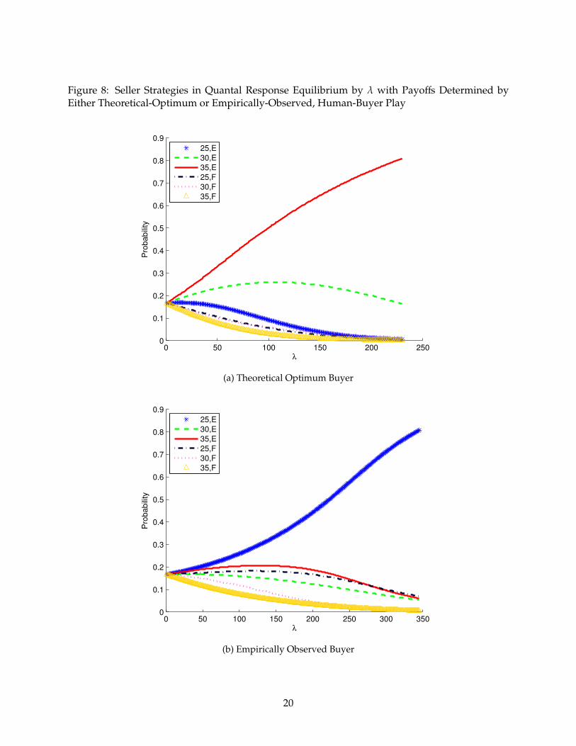
Figure 8: Seller Strategies in Quantal Response Equilibrium by λ with Payoffs Determined byEither Theoretical-Optimum or Empirically-Observed, Human-Buyer Play

0 50 100 150 200 2500

0.1

0.2

0.3

0.4

0.5

0.6

0.7

0.8

0.9P

robabili

ty

λ

25,E

30,E

35,E

25,F

30,F

35,F

(a) Theoretical Optimum Buyer

0 50 100 150 200 250 300 3500

0.1

0.2

0.3

0.4

0.5

0.6

0.7

0.8

0.9

Pro

babili

ty

λ

25,E

30,E

35,E

25,F

30,F

35,F

(b) Empirically Observed Buyer

20

δ term in the first and last periods of the human buyer treatment, respectively; the terms δC0, and

δCT represent the δ term in the first and last periods of the computer-buyer treatment, respectively.

All other periods are convex combinations of their respective treatments’ two terms. Similar terms

are constructed for λ in the QRE model: λH0, λHT, λC0, and λCT. Equation (8) provides this utility

model for subject i in period t.

uit (sit) =

(20 − p

19uX0 (sit) +

p − 119

uXT (sit))

(8)

X ∈ {C,H} represents two treatments.

where

uC0 (sit) = λC0

∑−i

u (sit, s−i) Prob (s−i) + δC0I(exploding offer)

uCT (sit) = λCT

∑−i

u (sit, s−i) Prob (s−i) + δCTI(exploding offer)

uH0 (sit) = λH0

∑−i

u (sit, s−i) Prob (s−i) + δH0I(exploding offer)

uHT (sit) = λHT

∑−i

u (sit, s−i) Prob (s−i) + δHTI(exploding offer)

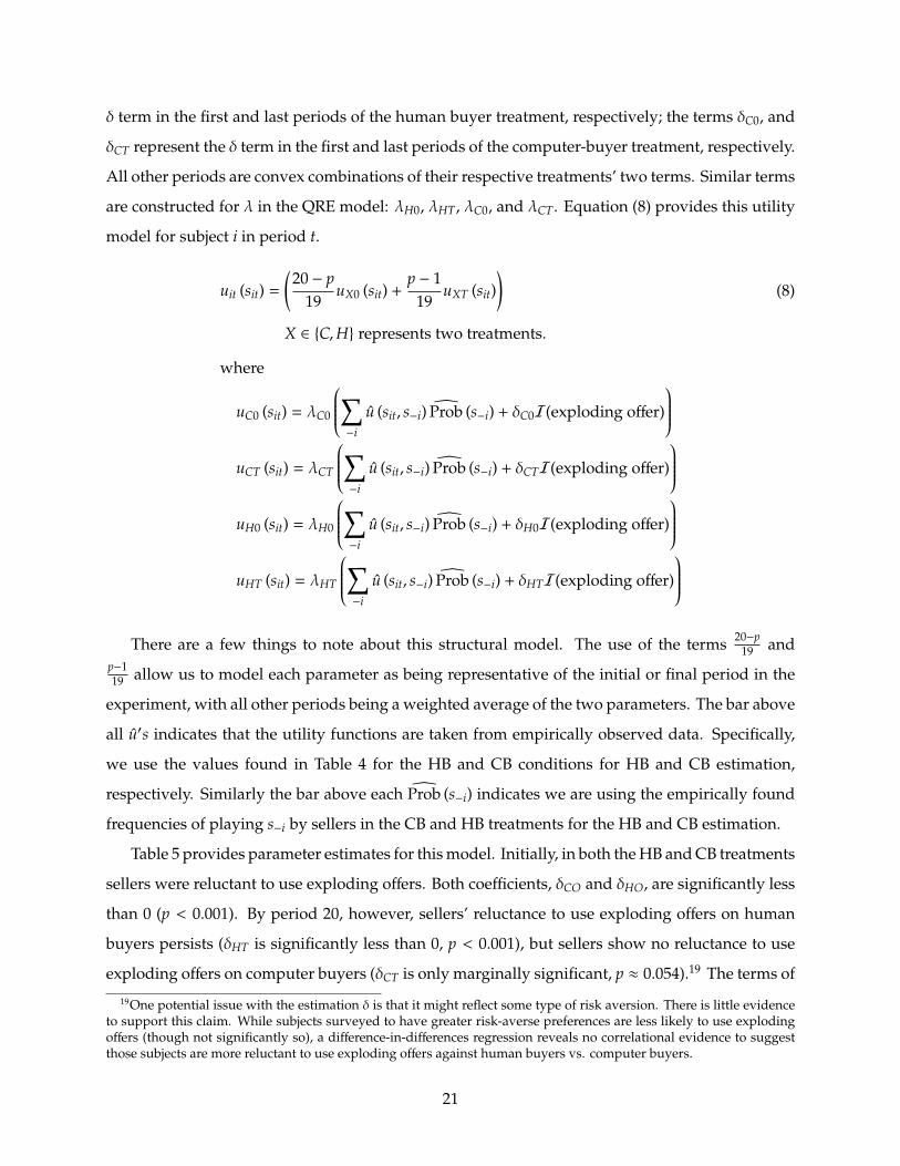
There are a few things to note about this structural model. The use of the terms 20−p

19 andp−119 allow us to model each parameter as being representative of the initial or final period in the

experiment, with all other periods being a weighted average of the two parameters. The bar above

all u′s indicates that the utility functions are taken from empirically observed data. Specifically,

we use the values found in Table 4 for the HB and CB conditions for HB and CB estimation,

respectively. Similarly the bar above each Prob (s−i) indicates we are using the empirically found

frequencies of playing s−i by sellers in the CB and HB treatments for the HB and CB estimation.

Table 5 provides parameter estimates for this model. Initially, in both the HB and CB treatments

sellers were reluctant to use exploding offers. Both coefficients, δCO and δHO, are significantly less

than 0 (p < 0.001). By period 20, however, sellers’ reluctance to use exploding offers on human

buyers persists (δHT is significantly less than 0, p < 0.001), but sellers show no reluctance to use

exploding offers on computer buyers (δCT is only marginally significant, p ≈ 0.054).19 The terms of

19One potential issue with the estimation δ is that it might reflect some type of risk aversion. There is little evidenceto support this claim. While subjects surveyed to have greater risk-averse preferences are less likely to use explodingoffers (though not significantly so), a difference-in-differences regression reveals no correlational evidence to suggestthose subjects are more reluctant to use exploding offers against human buyers vs. computer buyers.

21

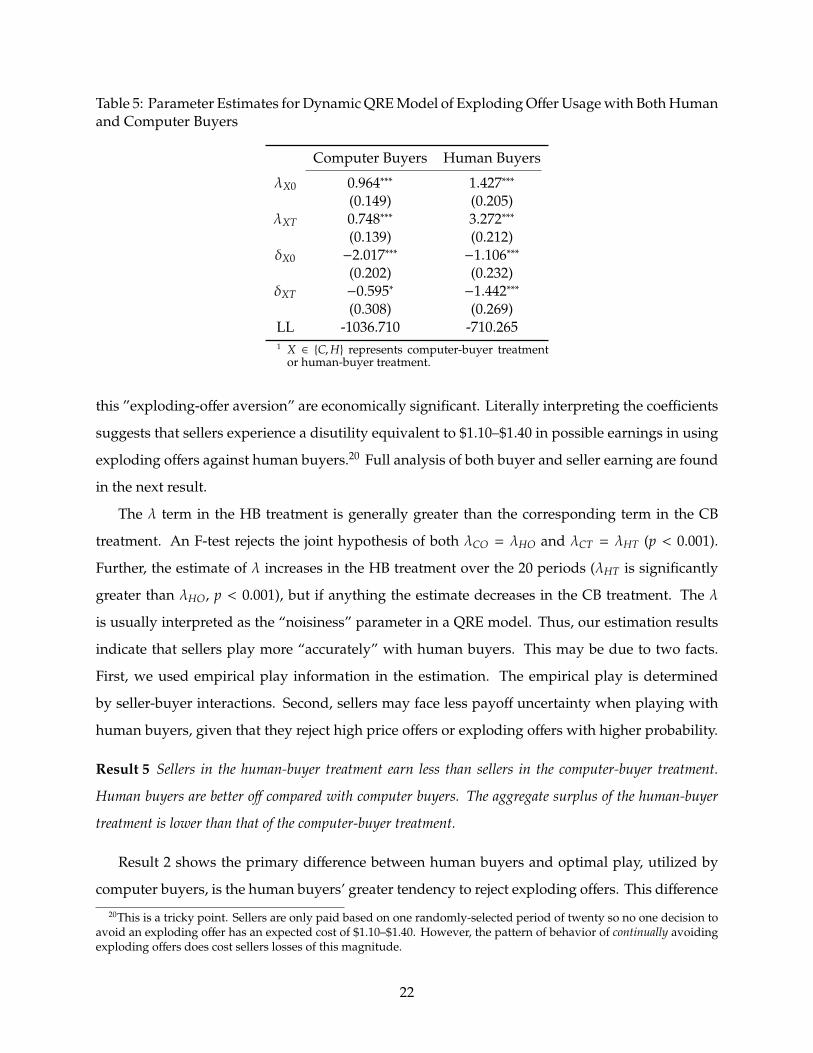
Table 5: Parameter Estimates for Dynamic QRE Model of Exploding Offer Usage with Both Humanand Computer Buyers

Computer Buyers Human Buyers

λX0 0.964∗∗∗ 1.427∗∗∗

(0.149) (0.205)λXT 0.748∗∗∗ 3.272∗∗∗

(0.139) (0.212)δX0 −2.017∗∗∗ −1.106∗∗∗

(0.202) (0.232)δXT −0.595∗ −1.442∗∗∗

(0.308) (0.269)LL -1036.710 -710.2651 X ∈ {C,H} represents computer-buyer treatment

or human-buyer treatment.

this ”exploding-offer aversion” are economically significant. Literally interpreting the coefficients

suggests that sellers experience a disutility equivalent to $1.10–$1.40 in possible earnings in using

exploding offers against human buyers.20 Full analysis of both buyer and seller earning are found

in the next result.

The λ term in the HB treatment is generally greater than the corresponding term in the CB

treatment. An F-test rejects the joint hypothesis of both λCO = λHO and λCT = λHT (p < 0.001).

Further, the estimate of λ increases in the HB treatment over the 20 periods (λHT is significantly

greater than λHO, p < 0.001), but if anything the estimate decreases in the CB treatment. The λ

is usually interpreted as the “noisiness” parameter in a QRE model. Thus, our estimation results

indicate that sellers play more “accurately” with human buyers. This may be due to two facts.

First, we used empirical play information in the estimation. The empirical play is determined

by seller-buyer interactions. Second, sellers may face less payoff uncertainty when playing with

human buyers, given that they reject high price offers or exploding offers with higher probability.

Result 5 Sellers in the human-buyer treatment earn less than sellers in the computer-buyer treatment.

Human buyers are better off compared with computer buyers. The aggregate surplus of the human-buyer

treatment is lower than that of the computer-buyer treatment.

Result 2 shows the primary difference between human buyers and optimal play, utilized by

computer buyers, is the human buyers’ greater tendency to reject exploding offers. This difference

20This is a tricky point. Sellers are only paid based on one randomly-selected period of twenty so no one decision toavoid an exploding offer has an expected cost of $1.10–$1.40. However, the pattern of behavior of continually avoidingexploding offers does cost sellers losses of this magnitude.

22

10

11

12

13

14

15

16

17

18

Avera

ge P

rofit (U

SD

)

0 5 10 15 20Period

Computer Buyer Condition Human Buyer Condition

10

11

12

13

14

15

16

17

18

Avera

ge P

rofit (U

SD

)

0 5 10 15 20Period

Computer Buyer Condition Human Buyer Condition

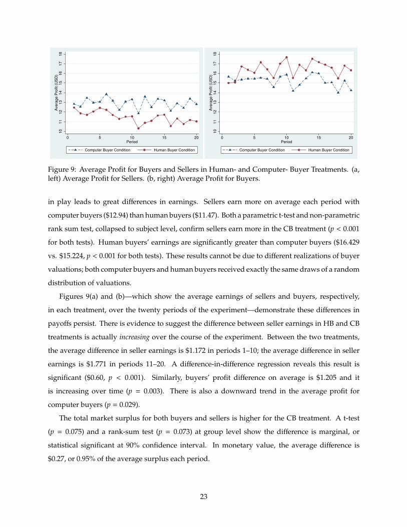
Figure 9: Average Profit for Buyers and Sellers in Human- and Computer- Buyer Treatments. (a,left) Average Profit for Sellers. (b, right) Average Profit for Buyers.

in play leads to great differences in earnings. Sellers earn more on average each period with

computer buyers ($12.94) than human buyers ($11.47). Both a parametric t-test and non-parametric

rank sum test, collapsed to subject level, confirm sellers earn more in the CB treatment (p < 0.001

for both tests). Human buyers’ earnings are significantly greater than computer buyers ($16.429

vs. $15.224, p < 0.001 for both tests). These results cannot be due to different realizations of buyer

valuations; both computer buyers and human buyers received exactly the same draws of a random

distribution of valuations.

Figures 9(a) and (b)—which show the average earnings of sellers and buyers, respectively,

in each treatment, over the twenty periods of the experiment—demonstrate these differences in

payoffs persist. There is evidence to suggest the difference between seller earnings in HB and CB

treatments is actually increasing over the course of the experiment. Between the two treatments,

the average difference in seller earnings is $1.172 in periods 1–10; the average difference in seller

earnings is $1.771 in periods 11–20. A difference-in-difference regression reveals this result is

significant ($0.60, p < 0.001). Similarly, buyers’ profit difference on average is $1.205 and it

is increasing over time (p = 0.003). There is also a downward trend in the average profit for

computer buyers (p = 0.029).

The total market surplus for both buyers and sellers is higher for the CB treatment. A t-test

(p = 0.075) and a rank-sum test (p = 0.073) at group level show the difference is marginal, or

statistical significant at 90% confidence interval. In monetary value, the average difference is

$0.27, or 0.95% of the average surplus each period.

23

5 Conclusion

This paper provides the first experimental investigation into methods of search deterrence in the

consumer goods market. Although theory (Armstrong and Zhou, 2013) suggests some form of

search deterrence is optimal for sellers in most conditions, our suspicion was that buyers might

respond negatively to such tactics, reducing the likelihood they would be used by sellers. Our

findings confirm this suspicion. Buyers reject exploding offers more often than is optimal. Sellers

use exploding offers less often than both the theoretical optimum and a profit-maximizing strategy

based on actual buyer behavior would dictate. Sellers do not demonstrate a similar tendency

with computer buyers, suggesting their aversion to exploding offers may be a preference-based

phenomenon and not the result of miscalculation.

The results of this experiment provide suggestive evidence as to why search deterrence in

consumer markets may not be as widespread as theory might suggest. Buyers simply do not like

exploding offers and reject them more than what profit-maximizing behavior would dictate. A

best-responding seller would have to take this into account and use exploding offers less often than

the theoretical optimum. Further, sellers who are exploding-offer averse, like in our experiment,

would use even fewer exploding offers.

The results and implications of this work fill a previously unexamined area in the literature.

Most theoretical and experimental work examine exploding offers in labor markets, where buyers

make exploding offers to sellers. For instance, in theoretical work, Lippman and Mamer (2012)

characterize under which conditions a buyer, seeking to purchase an asset from a seller, will use

exploding offers. In experimental work, Niederle and Roth (2009) show that matching markets

with exploding offers—together with binding acceptances—create early and dispersed transactions

and lower match quality. Lau et al. (forthcoming) find experimental employees hired through

exploding offers exhibit less effort for their employers, leading to welfare losses for both sides. Tang

et al. (2009) frame their experimental Ultimatum Deadline Game as a hiring problem. Proposers

offer responders some amount of time to make a decision. They find experimental proposers tend

to set deadlines that are too short, and their offers are frequently rejected. Only Armstrong and

Zhou (2013) explicitly model a consumer goods market. Their model, the theoretical basis for this

paper, involves sequential consumer search where multiple firms choose whether or not to use

exploding offers and set prices accordingly.

This paper also relates to experimental studies in sequential search markets. Early studies

24

in sequential search markets focus on the optimal stopping rule when individuals faced price or

wage offers (Schotter and Braunstein, 1981; Cox and Oaxaca, 1989; Kogut, 1990). Those experi-

ments evaluated individuals’ search behavior when uncertain price/wage offers follow a known

distribution and searching involves a constant search cost. They find that consumers tend to stop

earlier, compared with risk neutral consumers, who only care about marginal expected gains.

The literature naturally extends to more general experimental markets where sellers make price

offers and buyers make purchase decisions (Grether et al., 1988; Cason and Friedman, 2003). That

research involves testing equilibrium price and evaluating market performance. For example,

Cason and Friedman (2003) test “noisy search equilibrium” using both computer buyers and real

buyers. The paper builds on this strand of literature by augmenting traditional search experi-

mental designs with the possibility of exploding offers. Unlike the previous findings, the use of

exploding offers generally leads buyers to search longer than optimal, as buyers are more likely to

reject sellers’ exploding offers and continue their search.

Of course, one simplification we have made is using exploding offers as the only example

of search deterrence in our experiment. We specifically chose exploding offers rather than other

forms of search deterrence, because the strategy is the simplest form of search deference, an extreme

case of the model, and the one believed most likely to provoke a negative response from buyers.

Theory shows other search deterrence strategies are optimal in a greater variety of situations than

exploding offers (Armstrong and Zhou, 2013). We leave it as a future extension of our work to

experimentally investigate buyers’ response to such search deterrence.

References

Mark Armstrong and Jidong Zhou. Search deterrence. Working Paper, University of Oxford, 2013.

Christopher Avery, Christine Jolls, Richard A. Posner, and Alvin E. Roth. The market for federal

judicial law clerks. The University of Chicago Law Review, 68(3):793–902, 2001.

Christopher Avery, Christine Jolls, Richard A. Posner, and Alvin E. Roth. The new market for

federal judicial law clerks. The University of Chicago Law Review, 74(2):447–486, 2007.

Yaron Azrieli, Christopher P. Chambers, and Paul J. Healy. Incentives in experiments: A theoretical

analysis. 2014.

Colin F. Camerer. Behavioral Game Theory. Princeton University Press, 2003.

25

Timothy N. Cason and Daniel Friedman. Buyer search and price dispersion: a laboratory study.

Journal of Economic Theory, 112(2):232–260, 2003.

James C. Cox and Ronald L. Oaxaca. Laboratory experiments with a finite-horizon job-search

model. Journal of Risk and Uncertainty, 2(3):301–329, 1989.

Catherine C. Eckel and Philip J. Grossman. Forecasting risk attitudes: An experimental study

using actual and forecast gamble choices. Journal of Economic Behavior & Organization, 68(1):1 –

17, 2008.

Urs Fischbacher. z-tree: Zurich toolbox for ready-made economic experiments. Experimental

Economics, 10(2):171–178, 2007.

Shane Frederick. Cognitive reflection and decision making. Journal of Economic Perspectives, 19(4):

25–42, 2005.

Ben Greiner. The online recruitment system ORSEE 2.0 - a guide for the organization of experiments

in economics. University of Cologne, 2004.

David M. Grether, Alan Schwartz, and Louis L. Wilde. Uncertainty and shopping behaviour: An

experimental analysis. Review of Economic Studies, 55(2):323–42, 1988.

Carl A. Kogut. Consumer search behavior and sunk costs. Journal of Economic Behavior & Organi-

zation, 14(3):381–392, 1990.

Nelson Lau, Yakov Bart, Joseph Neil Bearden, and Ilia Tsetlin. Exploding offers can blow up in

more than one way. Decision Analysis, forthcoming.

Steven A. Lippman and John W. Mamer. Exploding offers. Decision Analysis, 9(1):6–21, 2012.

Richard D. McKelvey and Thomas R. Palfrey. Quantal response equilibria for normal form games.

Games and Economic Behavior, 10(1):6 – 38, 1995.

Richard D. McKelvey and Thomas R. Palfrey. Quantal response equilibria for extensive form

games. Experimental Economics, 1(1):9–41, 1998.

Muriel Niederle and Alvin E. Roth. Market culture: How rules governing exploding offers affect

market performance. American Economic Journal: Microeconomics, 1(2):199–219, 2009.

26

Alvin E Roth and Xiaolin Xing. Jumping the gun: Imperfections and institutions related to the

timing of market transactions. The American Economic Review, pages 992–1044, 1994.

Michael Rothschild. Searching for the lowest price when the distribution of prices is unknown.

The Journal of Political Economy, pages 689–711, 1974.

Andrew Schotter and Yale M. Braunstein. Economic search: An experimental study. Economic

Inquiry, 19(1):1–25, 1981.

George J Stigler. The economics of information. The journal of political economy, pages 213–225,

1961.

Wenjie Tang, J. Neil Bearden, and Ilia Tsetlin. Ultimatum deadlines. Management Science, 55(8):

1423–1437, 2009.

27