Exploiting Dynamic Phase Distance Mapping for

Phase-based Tuning of Embedded Systems

Tosiron Adegbija and Ann Gordon-Ross*

Department of Electrical and Computer Engineering

University of Florida, Gainesville, Florida, USA

*Also with the Center for High Performance Reconfigurable Computing (CHREC) at University of Florida

e-mail: tosironkbd@ufl.edu, ann@ece.ufl.edu

Abstract—Phase-based tuning increases optimization potential

by configuring system parameters for application execution

phases. Previous work proposed phase distance mapping

(PDM), which relied on extensive a priori analysis of executing

applications to dynamically estimate the best configuration

using the correlation between phases. We propose DynaPDM, a

new dynamic phase distance mapping methodology that

eliminates a priori designer effort, dynamically analyzes phases,

and determines the best configurations, yielding average energy

delay product savings of 28%—an 8% improvement on PDM—

and configurations within 1% of the optimal.

Keywords—Cache tuning, dynamic reconfiguration, phase-

based tuning, configurable hardware, energy delay product

savings

I. INTRODUCTION AND MOTIVATION

Due to the proliferation of embedded systems with

increasingly stringent design constraints (e.g., size, battery

capacity, cost, real-time deadlines, market competition, etc.),

extensive research has focused on system optimizations.

However, numerous tunable parameters/hardware (e.g., cache

size, associativity, and line size [21]; replacement policy [22],

issue width [5]; core voltage and frequency [18], etc.) and

tunable parameter values, combined with increasing numbers

of cores, results in an exponentially increasing design space,

making system optimization a daunting challenge. The

dynamic nature of applications further compounds these

challenges, requiring optimizations to dynamically configure

tunable parameter values at runtime to the best configuration

to most effectively meet design goals [12][20] and changing

application behavior.

Application execution can be partitioned into execution

intervals and intervals with similar and stable characteristics

(e.g., cache misses, instructions per cycle (IPC), branch

mispredictions, etc.) can be grouped as phases. Same-phased

intervals tend to have the same best configurations and phase-

based tuning specializes the system’s configurations to the

application’s phases’ requirements. To facilitate phase-based

tuning, phase classification [20] clusters intervals with similar

characteristics using methods such as K-means clustering [16]

or Markov predictors [20].

A significant challenge for phase-based tuning is

determining the best configurations without incurring

significant tuning overhead (e.g., power, performance,

energy). Exhaustive search methods [21] incur significant

tuning overhead by physically executing all configurations

and selecting the best configuration. Heuristic methods [10]

execute a fraction of the design space, but still incur tuning

overhead. Analytical methods [7] directly determine,

calculate, or predict the best configuration based on the design

constraints and the application’s characteristics, incurring no

tuning overhead, however, most of these methods are either

computationally complex or not dynamic.

To make analytical methods more amenable to dynamic

(runtime) phase-based tuning, phase distance mapping (PDM)

[1] used a computationally simple, dynamic analytical model

that leveraged phase distances to directly estimate the best

configuration with no design space exploration and minimal

tuning overhead. Even though results showed that PDM

achieved significant energy delay product (EDP) savings, the

designer was still required to statically pre-analyze the

applications, applications’ phases, and configurations to

provide information for runtime PDM decisions. These design

time steps required considerable designer effort and a priori

knowledge of the applications, which limits PDM’s

applicability, precluding applications with many phases and

general purpose systems with unknown applications (e.g.,

smartphones).

In this work, we introduce a new methodology for PDM—

DynaPDM—which addresses PDM’s limitations by

dynamically analyzing applications, applications’ phases, and

configurations, thereby eliminating designer effort while

maintaining the computational simplicity, low tuning

overhead, and phase-based fundamentals of PDM. We directly

compare DynaPDM and PDM with respect to cache tuning for

configurable size, line size, and associativity, and use cache

miss rates to classify application phases, however,

DynaPDM’s fundamentals are applicable to any tunable

hardware. Results reveal that DynaPDM determines

configurations within 1% of the optimal (lowest EDP)

configuration and achieves average system-wide EDP savings

of 28%. DynaPDM improves EDP savings over PDM by 8%,

and most importantly, eliminates the design time effort

required by PDM where the EDP savings are directly

dependent on the designer’s a priori phase analysis.

II. RELATED WORK

Since PDM was evaluated using cache tuning, we focus

our related work discussions to that optimization domain, but

note that there is extensive prior work in phase-based tuning

for other system parameters (e.g., [13][18][19], etc.). Zhang et

al. [21] proposed a configurable cache architecture that

determined the Pareto optimal cache configurations trading off

energy consumption and performance. Zou et al. [22]

proposed a configuration management algorithm to search the

design space for the best cache configurations. However, these

methods incurred significant tuning overhead by physically

exploring the design space.

To reduce tuning overhead, several methods eliminated

design space exploration. Gordon-Ross et al. [11] proposed a

one-shot approach to cache configuration that non-intrusively

predicted the best cache configuration using an oracle [14],

however, the oracle hardware introduced significant power

overhead when active. Ghosh et al. [7] proposed an analytical

model to directly determine the best cache configuration based

on performance constraints and application characteristics,

however, the model’s computational complexity incurred

energy and performance overheads. Even though these

methods reduced the tuning overhead, these methods were not

phase-based.

Hajimir et al. [12] used a cache model for phase-based

tuning that used changes in application characteristics to

determine when to change the cache configuration and

presented a dynamic programming-based algorithm to find the

optimal cache configurations. Gordon-Ross et al. [8]

investigated the benefits of phase-based tuning over

application-based tuning (using a single configuration for the

entire application execution) with respect to energy

consumption and performance, and quantified the tuning

overhead due to cache flushing and write backs, which was

minimal. Phase-based tuning yielded improvements of up to

37% in performance and 20% in energy over application-

based tuning. However, to maximize phase-based tuning

savings, phase changes must be quickly detected and phases

accurately characterized/classified [9].

Phase classification partitions application execution into

intervals, measured by the number of instructions executed,

and intervals showing similar characteristics are clustered into

phases. Even though phase classification can be done offline,

online phase classification more accurately characterizes

dynamic application phase behavior [20]. Dhodapkar et al. [4]

found a relationship between phases and the interval’s

working set (i.e., address access locality), and concluded that

phase changes could be detected using changes in the working

set. Balasubramonian et al. [2] used cache miss rates, cycles

per instruction (CPI), and branch frequency to detect phase

changes for cache tuning.

III. PHASE DISTANCE MAPPING (PDM)

A. PDM Overview and Limitations

Since our work leverages prior fundamentals established

by PDM [1], we first give an overview of PDM and define the

key terminology. The phase distance is the difference between

the characteristics of a characterized phase—phase with a

known best configuration—and an uncharacterized phase and

is used to estimate the uncharacterized phase’s best

configuration. PDM compared a single previously

characterized phase—the base phase—with a new phase to

determine the phase distance. PDM used the phase distance to

calculate the configuration distance—the difference between

the tunable parameter values of two configurations. Finally,

distance windows define phase distance ranges and the

corresponding tunable parameter values. The distance window

that the phase distance falls within (i.e., maps to) defines the

tunable parameter values (i.e., best configuration) for the

uncharacterized phase.

Even though PDM showed good average EDP savings,

PDM had several limitations. First, the designer was required

to statically define the distance windows based on the

anticipated applications, which limits PDM’s applicability to

dynamic systems where applications are not known a priori.

PDM also required the designer to designate the base phase

such that the base phase represented the system’s prominent

application domain. Results showed that PDM’s EDP savings

were strongly affected by how well the base phase represented

the entire system.

In the remainder of this section, we detail our major

contributions with respect to PDM. We introduce DynaPDM,

which alleviates all design time effort and maximizes EDP

savings by defining distance windows during runtime and

dynamically designating the base phase and calculating the

associated configuration distances, thus specializing the

distance windows to dynamic system and application

behavior.

B. Design Space and Phase-based Tuning Architecture

Our memory hierarchy consists of configurable, private

level one (L1) instruction and data caches. The caches have a

base size of 8 Kbytes with four 2 Kbyte configurable banks,

which can be shut down and/or concatenated to tune the cache

size and associativity, and a base line size of 16 bytes, which

can be increased by fetching multiple lines [21]. To quantify

EDP savings as compared to a non-configurable cache, we

compared to a base cache configuration of 8 Kbytes with 4-

way set associativity and a 64 byte line size, which represents

an average configuration on a typical embedded

microprocessor suitable for our experimental applications

[21]. Given this base cache, the design space contains all

combinations of cache sizes, associativities, and line sizes

ranging from 2 to 8 Kbytes, direct-mapped to 4-way, and 16 to

64 bytes, respectively.

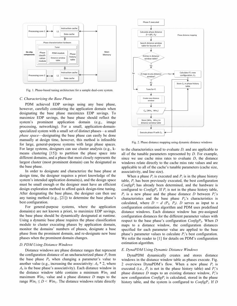
Fig. 1 depicts the phase-based tuning architecture for a

sample dual-core system, which can be extended to any n-core

system. Each core has private L1 instruction and data caches

connected to the phase characterization hardware, which

consists of a tuner to orchestrate the tuning process by

gathering cache statistics and calculating the EDP, a phase

classification module to classify the application phases, a

phase history table to store the history of the characterized

phases and associated best configurations, and a PDM module.

The PDM module contains a distance window table to store

the distance windows and serves as a lookup table for the

configuration distances when phases are characterized. Prior

research using similar table structures showed that these

structures contribute negligible area, performance, and energy

overheads [20].

C. Characterizing the Base Phase

PDM achieved EDP savings using any base phase,

however, carefully considering the application domain when

designating the base phase maximizes EDP savings. To

maximize EDP savings, the base phase should reflect the

system’s prominent application domain (e.g., image

processing, networking). For a small, application-domain-

specialized system with a small set of distinct phases—a small

phase space—designating the base phase can easily be done

manually at design time, however, this method is infeasible

for large, general-purpose systems with large phase spaces.

For large systems, designers can use cluster analysis (e.g., k-

means clustering [15]) to partition the phase space into

different domains, and a phase that most closely represents the

largest cluster (most prominent domain) can be designated as

the base phase.

In order to designate and characterize the base phase at

design time, the designer requires a priori knowledge of the

system’s intended application domain(s), and the design space

must be small enough or the designer must have an efficient

design exploration method to afford quick design-time tuning.

After designating the base phase, the designer can then use

any tuning method (e.g., [21]) to determine the base phase’s

best configuration.

For general-purpose systems, where the application

domain(s) are not known a priori, to maximize EDP savings,

the base phase should be dynamically designated at runtime.

Using a dynamic base phase requires the phase classification

module to cluster executing phases by application domain,

monitor the domains’ numbers of phases, designate a base

phase from the prominent domain, and re-designate new base

phases when the prominent domain changes.

D. PDM Using Distance Windows

Distance windows are phase distance ranges that represent

the configuration distance of an uncharacterized phase Pi from

the base phase Pb when changing a parameter’s value to

another value (e.g., increasing the associativity: Ab * 2, where

Ab is the base phase’s associativity). Each distance window in

the distance window table contains a minimum WinL and

maximum WinU value and a phase distance D maps to the

range WinL ≤ D < WinU. The distance windows relate directly

to the characteristics used to evaluate D, and are applicable to

all of the tunable parameters represented by D. For example,

since we use cache miss rates to evaluate D, the distance

windows relate directly to the cache miss rate values and are

applicable to all of the cache’s tunable parameters (cache size,

associativity, and line size).

When a phase Pi is executed and Pi is in the phase history

table, Pi has been previously executed, the best configuration

ConfigPi has already been determined, and the hardware is

configured to ConfigPi. If Pi is not in the phase history table,

Pi is a new phase and the phase distance D between Pi’s

characteristics and the base phase Pb’s characteristics is

calculated, where D = d (Pb, Pi). D serves as input to a

configuration estimation algorithm and PDM uses predefined

distance windows. Each distance window has pre-assigned

configuration distances for the different parameter values with

respect to the base phase’s configuration ConfigPb. When D

maps to a distance window, the configuration distances

specified for each parameter value are applied to the base

phase’s parameter values to calculate Pi’s best configuration.

We refer the reader to [1] for details on PDM’s configuration

estimation algorithm.

E. DynaPDM Using Dynamic Distance Windows

DynaPDM dynamically creates and stores distance

windows in the distance window table as phases execute. Fig.

2 overviews DynaPDM’s flow. When a new phase Pi is

executed (i.e., Pi is not in the phase history table) and Pi’s

phase distance D maps to an existing distance window, Pi’s

new configuration ConfigPi is calculated, stored in the phase

history table, and the system is configured to ConfigPi. If D

Phase Pi executed

Calculate phase distanceD = d(Pi, Pb)

D maps to any distance window?

Search distance window table for bounds of D

Calculate Pi’s new configuration, CPi

Yes

Store CPi in phase history table

Create new distance window

No

Cpi, [WinL, WinU)

Store [WinL, WinU) in distance window table

Phase distance mapping

Execute phase Pi with CPi

Tune for Pi

Entries in distance window table?

Yes

No

Fig. 2. Phase distance mapping using dynamic distance windows

Processing core 1

Processing core 2

Main Memory

Instruction cache

Data cacheL1

Instruction cache

Data cacheL1

Phase history table

Phase classifi-cation

module

Tuner

Phase characterization hardware

On-chip components

PDM module

Distance window table

Fig. 1. Phase-based tuning architecture for a sample dual-core system.

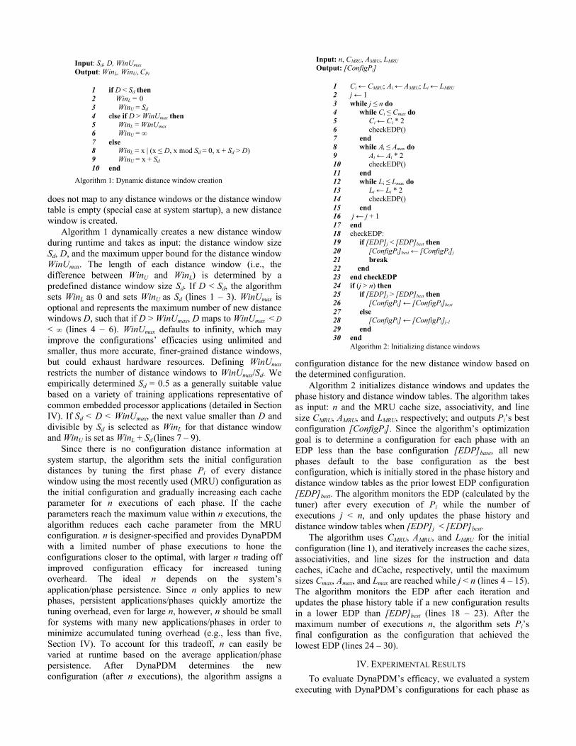
does not map to any distance windows or the distance window

table is empty (special case at system startup), a new distance

window is created.

Algorithm 1 dynamically creates a new distance window

during runtime and takes as input: the distance window size

Sd, D, and the maximum upper bound for the distance window

WinUmax. The length of each distance window (i.e., the

difference between WinU and WinL) is determined by a

predefined distance window size Sd. If D < Sd, the algorithm

sets WinL as 0 and sets WinU as Sd (lines 1 – 3). WinUmax is

optional and represents the maximum number of new distance

windows D, such that if D > WinUmax, D maps to WinUmax < D

< ∞ (lines 4 – 6). WinUmax defaults to infinity, which may

improve the configurations’ efficacies using unlimited and

smaller, thus more accurate, finer-grained distance windows,

but could exhaust hardware resources. Defining WinUmax

restricts the number of distance windows to WinUmax/Sd. We

empirically determined Sd = 0.5 as a generally suitable value

based on a variety of training applications representative of

common embedded processor applications (detailed in Section

IV). If Sd < D < WinUmax, the next value smaller than D and

divisible by Sd is selected as WinL for that distance window

and WinU is set as WinL + Sd (lines 7 – 9).

Since there is no configuration distance information at

system startup, the algorithm sets the initial configuration

distances by tuning the first phase Pi of every distance

window using the most recently used (MRU) configuration as

the initial configuration and gradually increasing each cache

parameter for n executions of each phase. If the cache

parameters reach the maximum value within n executions, the

algorithm reduces each cache parameter from the MRU

configuration. n is designer-specified and provides DynaPDM

with a limited number of phase executions to hone the

configurations closer to the optimal, with larger n trading off

improved configuration efficacy for increased tuning

overheard. The ideal n depends on the system’s

application/phase persistence. Since n only applies to new

phases, persistent applications/phases quickly amortize the

tuning overhead, even for large n, however, n should be small

for systems with many new applications/phases in order to

minimize accumulated tuning overhead (e.g., less than five,

Section IV). To account for this tradeoff, n can easily be

varied at runtime based on the average application/phase

persistence. After DynaPDM determines the new

configuration (after n executions), the algorithm assigns a

configuration distance for the new distance window based on

the determined configuration.

Algorithm 2 initializes distance windows and updates the

phase history and distance window tables. The algorithm takes

as input: n and the MRU cache size, associativity, and line

size CMRU, AMRU, and LMRU, respectively; and outputs Pi’s best

configuration [ConfigPi]. Since the algorithm’s optimization

goal is to determine a configuration for each phase with an

EDP less than the base configuration [EDP]base, all new

phases default to the base configuration as the best

configuration, which is initially stored in the phase history and

distance window tables as the prior lowest EDP configuration

[EDP]best. The algorithm monitors the EDP (calculated by the

tuner) after every execution of Pi while the number of

executions j < n, and only updates the phase history and

distance window tables when [EDP]j < [EDP]best.

The algorithm uses CMRU, AMRU, and LMRU for the initial

configuration (line 1), and iteratively increases the cache sizes,

associativities, and line sizes for the instruction and data

caches, iCache and dCache, respectively, until the maximum

sizes Cmax, Amax, and Lmax are reached while j < n (lines 4 – 15).

The algorithm monitors the EDP after each iteration and

updates the phase history table if a new configuration results

in a lower EDP than [EDP]best (lines 18 – 23). After the

maximum number of executions n, the algorithm sets Pi’s

final configuration as the configuration that achieved the

lowest EDP (lines 24 – 30).

IV. EXPERIMENTAL RESULTS

To evaluate DynaPDM’s efficacy, we evaluated a system

executing with DynaPDM’s configurations for each phase as

Input: Sd, D, WinUmax

Output: WinL, WinU, CPi

1 if D < Sd then

2 WinL = 0

3 WinU = Sd

4 else if D > WinUmax then

5 WinL = WinUmax

6 WinU = ∞

7 else

8 WinL = x | (x ≤ D, x mod Sd = 0, x + Sd > D)

9 WinU = x + Sd

10 end

Algorithm 1: Dynamic distance window creation

Input: n, CMRU, AMRU, LMRU

Output: [ConfigPi]

1 Ci ← CMRU; Ai ← AMRU; Li ← LMRU

2 j ← 1

3 while j ≤ n do 4 while Ci ≤ Cmax do

5 Ci ← Ci * 2

6 checkEDP()

7 end 8 while Ai ≤ Amax do

9 Ai ← Ai * 2 10 checkEDP()

11 end 12 while Li ≤ Lmax do 13 Li ← Li * 2

14 checkEDP()

15 end

16 j ← j + 1

17 end

18 checkEDP:

19 if [EDP]j < [EDP]best then

20 [ConfigPi]best ← [ConfigPi]j

21 break 22 end

23 end checkEDP 24 if (j > n) then 25 if [EDP]j > [EDP]best then

26 [ConfigPi] ← [ConfigPi]best

27 else 28 [ConfigPi] ← [ConfigPi]j-1

29 end

30 end Algorithm 2: Initializing distance windows

compared to the optimal system executing the optimal

configuration for each phase (determined by exhaustive

search), and a system fixed with the base cache configuration.

We also implemented PDM in order to provide a direct

comparison with prior work.

A. Experimental Setup

To provide a fair comparison with PDM, we modeled our

experiments as closely with PDM as possible. We used the

same combination of sixteen workloads from the EEMBC

Multibench benchmark suite [6], which is an extensive suite

of multicore benchmarks that primarily model a wide variety

of realistic embedded systems. Each workload was a

collection of compute kernels processing a specific dataset

and included domains such as image processing, networking,

md5 checksum calculation, Huffman decoding, etc., with

image processing as the prominent domain. Since each

workload was a collection of specific compute kernels, each

of which performed a single task or a combination of similar

tasks, the kernels essentially represented a single phase of

execution. Therefore, without loss of generality, we assumed

that each workload represented a different phase.

We simulated the system using Perl scripts for each phase

to completion for the optimal, base, PDM, and DynaPDM

configurations for all executions of each phase. To collect

cache miss rates, we used the same homogeneous dual-core

system used for PDM with separate, private L1 instruction and

data caches modeled with GEM5 [3] and used McPAT [17] to

calculate the system’s total power consumption. We evaluated

the energy efficiency using the EDP,in Joule seconds:

EDP = system_power * phase_running_time2

= system_power * (total_phase_cycles/system_frequency)2

where system_power includes the core and cache powers and

total_phase_cycles is the total number of cycles to execute a

phase to completion.

B. Results

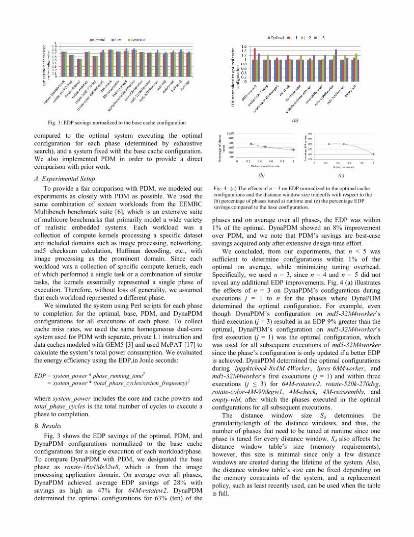
Fig. 3 shows the EDP savings of the optimal, PDM, and

DynaPDM configurations normalized to the base cache

configurations for a single execution of each workload/phase.

To compare DynaPDM with PDM, we designated the base

phase as rotate-16x4Ms32w8, which is from the image

processing application domain. On average over all phases,

DynaPDM achieved average EDP savings of 28% with

savings as high as 47% for 64M-rotatew2. DynaPDM

determined the optimal configurations for 63% (ten) of the

phases and on average over all phases, the EDP was within

1% of the optimal. DynaPDM showed an 8% improvement

over PDM, and we note that PDM’s savings are best-case

savings acquired only after extensive design-time effort.

We concluded, from our experiments, that n < 5 was

sufficient to determine configurations within 1% of the

optimal on average, while minimizing tuning overhead.

Specifically, we used n = 3, since n = 4 and n = 5 did not

reveal any additional EDP improvements. Fig. 4 (a) illustrates

the effects of n = 3 on DynaPDM’s configurations during

executions j = 1 to n for the phases where DynaPDM

determined the optimal configuration. For example, even

though DynaPDM’s configuration on md5-32M4worker’s

third execution (j = 3) resulted in an EDP 9% greater than the

optimal, DynaPDM’s configuration on md5-32M4worker’s

first execution (j = 1) was the optimal configuration, which

was used for all subsequent executions of md5-32M4worker

since the phase’s configuration is only updated if a better EDP

is achieved. DynaPDM determined the optimal configurations

during ipppktcheck-8x4M-4Worker, ipres-6M4worker, and

md5-32M4worker’s first executions (j = 1) and within three

executions (j ≤ 3) for 64M-rotatew2, rotate-520k-270deg,

rotate-color-4M-90degw1, 4M-check, 4M-reassembly, and

empty-wld, after which the phases executed in the optimal

configurations for all subsequent executions.

The distance window size Sd determines the

granularity/length of the distance windows, and thus, the

number of phases that need to be tuned at runtime since one

phase is tuned for every distance window. Sd also affects the

distance window table’s size (memory requirements),

however, this size is minimal since only a few distance

windows are created during the lifetime of the system. Also,

the distance window table’s size can be fixed depending on

the memory constraints of the system, and a replacement

policy, such as least recently used, can be used when the table

is full.

Fig. 3: EDP savings normalized to the base cache configuration

(a)

(b) (c)

Fig. 4: (a) The effects of n = 3 on EDP normalized to the optimal cache

configurations and the distance window size tradeoffs with respect to the

(b) percentage of phases tuned at runtime and (c) the percentage EDP savings compared to the base configuration.

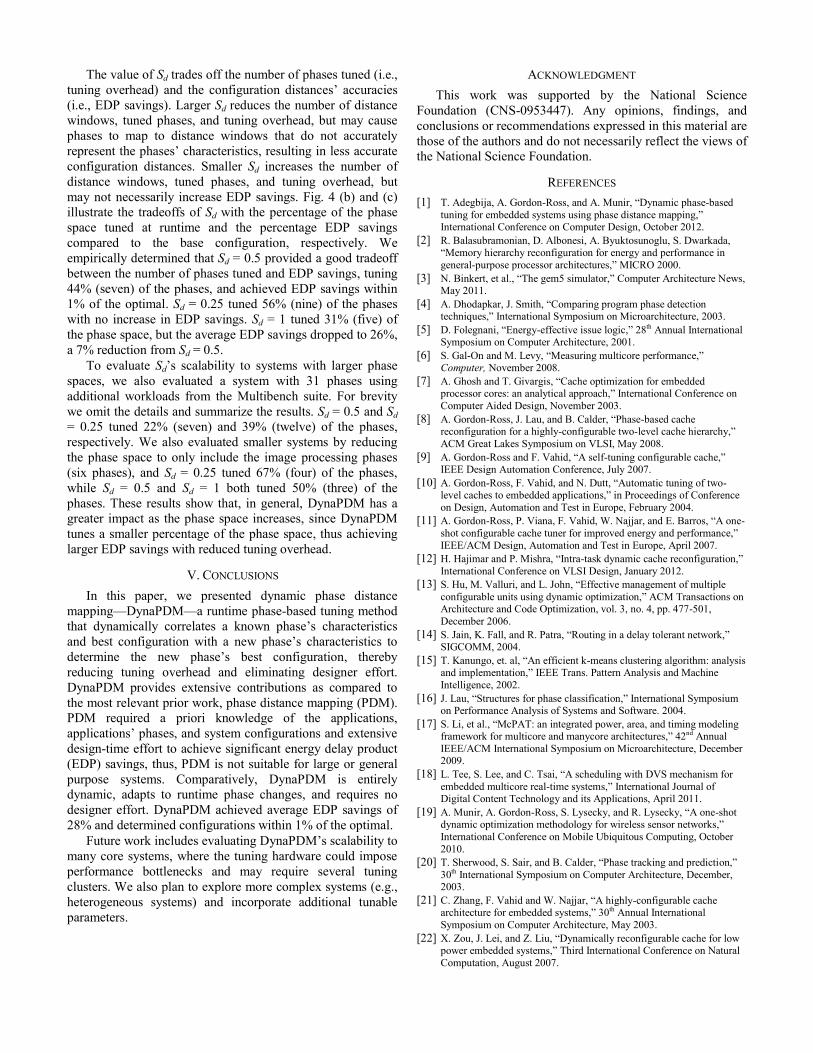
The value of Sd trades off the number of phases tuned (i.e.,

tuning overhead) and the configuration distances’ accuracies

(i.e., EDP savings). Larger Sd reduces the number of distance

windows, tuned phases, and tuning overhead, but may cause

phases to map to distance windows that do not accurately

represent the phases’ characteristics, resulting in less accurate

configuration distances. Smaller Sd increases the number of

distance windows, tuned phases, and tuning overhead, but

may not necessarily increase EDP savings. Fig. 4 (b) and (c)

illustrate the tradeoffs of Sd with the percentage of the phase

space tuned at runtime and the percentage EDP savings

compared to the base configuration, respectively. We

empirically determined that Sd = 0.5 provided a good tradeoff

between the number of phases tuned and EDP savings, tuning

44% (seven) of the phases, and achieved EDP savings within

1% of the optimal. Sd = 0.25 tuned 56% (nine) of the phases

with no increase in EDP savings. Sd = 1 tuned 31% (five) of

the phase space, but the average EDP savings dropped to 26%,

a 7% reduction from Sd = 0.5.

To evaluate Sd’s scalability to systems with larger phase

spaces, we also evaluated a system with 31 phases using

additional workloads from the Multibench suite. For brevity

we omit the details and summarize the results. Sd = 0.5 and Sd

= 0.25 tuned 22% (seven) and 39% (twelve) of the phases,

respectively. We also evaluated smaller systems by reducing

the phase space to only include the image processing phases

(six phases), and Sd = 0.25 tuned 67% (four) of the phases,

while Sd = 0.5 and Sd = 1 both tuned 50% (three) of the

phases. These results show that, in general, DynaPDM has a

greater impact as the phase space increases, since DynaPDM

tunes a smaller percentage of the phase space, thus achieving

larger EDP savings with reduced tuning overhead.

V. CONCLUSIONS

In this paper, we presented dynamic phase distance

mapping—DynaPDM—a runtime phase-based tuning method

that dynamically correlates a known phase’s characteristics

and best configuration with a new phase’s characteristics to

determine the new phase’s best configuration, thereby

reducing tuning overhead and eliminating designer effort.

DynaPDM provides extensive contributions as compared to

the most relevant prior work, phase distance mapping (PDM).

PDM required a priori knowledge of the applications,

applications’ phases, and system configurations and extensive

design-time effort to achieve significant energy delay product

(EDP) savings, thus, PDM is not suitable for large or general

purpose systems. Comparatively, DynaPDM is entirely

dynamic, adapts to runtime phase changes, and requires no

designer effort. DynaPDM achieved average EDP savings of

28% and determined configurations within 1% of the optimal.

Future work includes evaluating DynaPDM’s scalability to

many core systems, where the tuning hardware could impose

performance bottlenecks and may require several tuning

clusters. We also plan to explore more complex systems (e.g.,

heterogeneous systems) and incorporate additional tunable

parameters.

ACKNOWLEDGMENT

This work was supported by the National Science

Foundation (CNS-0953447). Any opinions, findings, and

conclusions or recommendations expressed in this material are

those of the authors and do not necessarily reflect the views of

the National Science Foundation.

REFERENCES

[1] T. Adegbija, A. Gordon-Ross, and A. Munir, “Dynamic phase-based

tuning for embedded systems using phase distance mapping,” International Conference on Computer Design, October 2012.

[2] R. Balasubramonian, D. Albonesi, A. Byuktosunoglu, S. Dwarkada, “Memory hierarchy reconfiguration for energy and performance in

general-purpose processor architectures,” MICRO 2000.

[3] N. Binkert, et al., “The gem5 simulator,” Computer Architecture News, May 2011.

[4] A. Dhodapkar, J. Smith, “Comparing program phase detection techniques,” International Symposium on Microarchitecture, 2003.

[5] D. Folegnani, “Energy-effective issue logic,” 28th Annual International

Symposium on Computer Architecture, 2001.

[6] S. Gal-On and M. Levy, “Measuring multicore performance,” Computer, November 2008.

[7] A. Ghosh and T. Givargis, “Cache optimization for embedded processor cores: an analytical approach,” International Conference on

Computer Aided Design, November 2003.

[8] A. Gordon-Ross, J. Lau, and B. Calder, “Phase-based cache reconfiguration for a highly-configurable two-level cache hierarchy,”

ACM Great Lakes Symposium on VLSI, May 2008.

[9] A. Gordon-Ross and F. Vahid, “A self-tuning configurable cache,” IEEE Design Automation Conference, July 2007.

[10] A. Gordon-Ross, F. Vahid, and N. Dutt, “Automatic tuning of two-level caches to embedded applications,” in Proceedings of Conference

on Design, Automation and Test in Europe, February 2004.

[11] A. Gordon-Ross, P. Viana, F. Vahid, W. Najjar, and E. Barros, “A one-

shot configurable cache tuner for improved energy and performance,”

IEEE/ACM Design, Automation and Test in Europe, April 2007.

[12] H. Hajimar and P. Mishra, “Intra-task dynamic cache reconfiguration,”

International Conference on VLSI Design, January 2012.

[13] S. Hu, M. Valluri, and L. John, “Effective management of multiple

configurable units using dynamic optimization,” ACM Transactions on Architecture and Code Optimization, vol. 3, no. 4, pp. 477-501,

December 2006.

[14] S. Jain, K. Fall, and R. Patra, “Routing in a delay tolerant network,” SIGCOMM, 2004.

[15] T. Kanungo, et. al, “An efficient k-means clustering algorithm: analysis and implementation,” IEEE Trans. Pattern Analysis and Machine

Intelligence, 2002.

[16] J. Lau, “Structures for phase classification,” International Symposium on Performance Analysis of Systems and Software. 2004.

[17] S. Li, et al., “McPAT: an integrated power, area, and timing modeling framework for multicore and manycore architectures,” 42nd Annual

IEEE/ACM International Symposium on Microarchitecture, December 2009.

[18] L. Tee, S. Lee, and C. Tsai, “A scheduling with DVS mechanism for

embedded multicore real-time systems,” International Journal of Digital Content Technology and its Applications, April 2011.

[19] A. Munir, A. Gordon-Ross, S. Lysecky, and R. Lysecky, “A one-shot dynamic optimization methodology for wireless sensor networks,”

International Conference on Mobile Ubiquitous Computing, October

2010.

[20] T. Sherwood, S. Sair, and B. Calder, “Phase tracking and prediction,”

30th International Symposium on Computer Architecture, December, 2003.

[21] C. Zhang, F. Vahid and W. Najjar, “A highly-configurable cache architecture for embedded systems,” 30th Annual International

Symposium on Computer Architecture, May 2003.

[22] X. Zou, J. Lei, and Z. Liu, “Dynamically reconfigurable cache for low power embedded systems,” Third International Conference on Natural

Computation, August 2007.