Exploiting Negative Curvature in Deterministic and ... Negative Curvature in Deterministic and ... in our deterministic algorithms and provide the ... Curvature in Deterministic and

Noname manuscript No.(will be inserted by the editor)

Exploiting Negative Curvature in Deterministic andStochastic Optimization

Frank E. Curtis · Daniel P. Robinson

April 3, 2018

Abstract This paper addresses the question of whether it can be beneficial for anoptimization algorithm to follow directions of negative curvature. Although priorwork has established convergence results for algorithms that integrate both descentand negative curvature steps, there has not yet been extensive numerical evidenceshowing that such methods offer consistent performance improvements. In thispaper, we present new frameworks for combining descent and negative curvaturedirections: alternating two-step approaches and dynamic step approaches. Theaspect that distinguishes our approaches from ones previously proposed is thatthey make algorithmic decisions based on (estimated) upper-bounding models ofthe objective function. A consequence of this aspect is that our frameworks can,in theory, employ fixed stepsizes, which makes the methods readily translatablefrom deterministic to stochastic settings. For deterministic problems, we showthat instances of our dynamic framework yield gains in performance comparedto related methods that only follow descent steps. We also show that gains canbe made in a stochastic setting in cases when a standard stochastic-gradient-typemethod might make slow progress.

Keywords nonconvex optimization · second-order methods · modified Newtonmethods · negative curvature · stochastic optimization · machine learning

Mathematics Subject Classification (2010) 49M05 · 49M15 · 49M37 · 65K05 ·90C15 · 90C26 · 90C30 · 90C53

F. E. CurtisDepartment of Industrial and Systems EngineeringLehigh UniversityE-mail: [email protected] author was supported in part by the U.S. Department of Energy under Grant No. DE-SC0010615 and by the U.S. National Science Foundation under Grant No. CCF-1618717.

D. P. RobinsonDepartment of Applied Mathematics and StatisticsJohns Hopkins UniversityE-mail: [email protected]

2 Frank E. Curtis, Daniel P. Robinson

1 Introduction

There has been a recent surge of interest in solving nonconvex optimization prob-lems. A prime example is the dramatic increase in interest in the training of deepneural networks. Another example is the task of clustering data that arise fromthe union of low dimensional subspaces. In this setting, the nonconvexity typicallyresults from sophisticated modeling approaches that attempt to accurately cap-ture corruptions in the data [5,13]. It is now widely accepted that the design ofnew methods for solving nonconvex problems (at least locally) is sorely needed.

First consider deterministic optimization problems. For solving such prob-lems, most algorithms designed for minimizing smooth objective functions onlyensure convergence to first-order stationarity, i.e., that the gradient of the objec-tive asymptotically vanishes. This characterization is certainly accurate for linesearch methods, which seek to reduce the objective function by searching alongdescent directions. Relatively few researchers have designed line search (or other,such as trust region or regularization) algorithms that generate iterates that prov-ably converge to second-order stationarity. The reason for this is three-fold: (i) suchmethods are more complicated and expensive, necessarily involving the computa-tion of directions of negative curvature when they exist; (ii) methods designed onlyto achieve first-order stationarity rarely get stuck at saddle points that are first-order, but not second-order stationary [19]; and (iii) there has not been sufficientevidence showing benefits of integrating directions of negative curvature.

For solving stochastic optimization problems, the methods most commonlyinvoked are variants of the stochastic gradient (SG) method. During each iterationof SG, a stochastic gradient is computed and a step opposite that direction is takento obtain the next iterate. Even for nonconvex problems, convergence guarantees(e.g., in expectation or almost surely) for SG methods to first-order stationarityhave been established under reasonable assumptions; e.g., see [2]. In fact, SG andits variants represent the current state-of-the-art for training deep neural networks.As for methods that compute and follow negative curvature directions, it is nosurprise that such methods (e.g., [20]) have not been used or studied extensivelysince practical benefits have not even been shown in deterministic optimization.

The main purpose of this paper is to revisit and provide new perspectives on theuse of negative curvature directions in deterministic and stochastic optimization.Whereas previous work in deterministic settings has focused on line search andother methods, we focus on methods that attempt to construct upper-bounding

models of the objective function. This allows them, at least in theory, to employfixed stepsizes while ensuring convergence guarantees. For a few instances of suchmethods of interest, we provide theoretical convergence guarantees and empiricalevidence showing that an optimization process can benefit by following negativecurvature directions. The fact that our methods might employ fixed stepsizes isalso important as it allows us to offer new strategies for stochastic optimizationwhere, e.g., line search strategies are not often viable.

1.1 Contributions

The contributions of our work are the following.

Exploiting Negative Curvature in Deterministic and Stochastic Optimization 3

– For deterministic optimization, we first provide conditions on descent and neg-ative curvature directions that allow us to guarantee convergence to second-order stationarity with a simple two-step iteration with fixed stepsizes; see §2.1.Using the two-step method as motivation, we then propose a dynamic choicefor the direction and stepsize; see §2.2. In particular, the dynamic algorithmmakes decisions based on which available step appears to offer a more signif-icant objective reduction. The details of our dynamic strategy represent themain novelty of this paper with respect to deterministic optimization.

– We prove convergence rate guarantees for our deterministic optimization meth-ods that provide upper bounds for the numbers of iterations required to achieve(approximate) first- and second-order stationarity; see §2.3. We follow this witha discussion, in §2.4, on the issue of how methods might behave in the neighbor-hood of so-called strict saddle points, a topic of much interest in the literature.

– In §2.5 and §2.6, we discuss different techniques for computing the search di-rections in our deterministic algorithms and provide the results of numericalexperiments showing the benefits of following negative curvature directions, asopposed to only descent directions.

– For solving stochastic optimization problems, we propose two methods. Ourfirst method shows that one can maintain the convergence guarantees of astochastic gradient method by adding an appropriately scaled negative curva-ture direction for a stochastic Hessian estimate; see §3.1. This approach can beseen as a refinement of that in [24], which adds noise to each SG step.

– Our second method for stochastic optimization is an adaptation of our dynamic(deterministic) method when stochastic gradient and Hessian estimates are in-volved; see §3.2. Although we are unable to establish a convergence theory forthis approach, we do illustrate some gain in performance in neural networktraining; see §3.3. We view this as a first step in the design of a practical algo-rithm for stochastic optimization that efficiently exploits negative curvature.

Computing directions of negative curvature carries an added cost that shouldbe taken into consideration when comparing algorithm performance. We remarkalong with the results of our numerical experiments how these added costs can beworthwhile and/or marginal relative to the other per-iteration costs.

1.2 Prior Related Work

For solving deterministic optimization problems, relatively little research has beendirected towards the use of negative curvature directions. Perhaps the first excep-tion is the work in [23] in which convergence to second-order stationary points isproved using a curvilinear search formed by descent and negative curvature di-rections. In a similar vein, the work in [6] offers similar convergence propertiesbased on using a curvilinear search, although the primary focus in that work isdescribing how a partial Cholesky factorization of the Hessian matrix could beused to compute descent and negative curvature directions. More recently, a linearcombination of descent and negative curvature directions was used in an opti-mization framework to establish convergence to second-order stationary solutionsunder loose assumptions [8,9], and a strategy for how to use descent and nega-tive curvature directions was combined with a backtracking linesearch to provide


worst case iteration bounds in [27]. For further instances of work employing nega-tive curvature directions, see [1,10,11,22]. Importantly, none of the papers above(or any others to the best of our knowledge) have established consistent gains incomputational performance as a result of using negative curvature directions.

Another recent trend in the design of deterministic methods for nonconvexoptimization is to focus on the ability of an algorithm to escape regions arounda saddle point, i.e., a first-order stationary point that is not a minimizer nor amaximizer. A prime example of this trend is the work in [26] in which a standardtype of regularized Newton method is considered. (For a more general presentationof regularized Newton methods of which the method in [26] is a special case,see, e.g., [25].) While the authors do show a probabilistic convergence result fortheir method to (approximate) second-order stationarity, their main emphasis ison the number of iterations required to escape neighborhoods of saddle points.This result, similar to those in some (but not all) recent papers discussing thebehavior of descent methods when solving nonconvex problems (e.g., see [14,19]),requires that all saddle points are non-degenerate in the sense that the Hessian ofthe objective at any such point does not have any zero eigenvalues. In particular,in [14] they show that a perturbed form of gradient descent converges to a second-order stationary point in a number iterations that depends poly-logarithmically onthe dimension of the problem. Our convergence theory does not require such a non-degeneracy assumption; see §2.4 for additional discussion comparing our resultsto others. (See also [18], where it is shown, without a non-degeneracy assumptionand for almost all starting points, that certain first-order methods do not convergeto saddle points at which the Hessian of the objective has a negative eigenvalue.That said, this work does not prove bounds on the number of iterations such amethod might spend near saddle points.)

For solving stochastic optimization problems, there has been little work thatfocuses explicitly on the use of directions of negative curvature. For two exam-ples, see [3,20]. Meanwhile, it has recently become clear that the nonconvex opti-mization problems used to train deep neural networks have a rich and interestinglandscape [4,15]. Instead of using negative curvature to their advantage, modernmethods ignore it, introduce random perturbations (e.g., see [7]), or employ reg-ularized/modified Newton methods that attempt to avoid its potential ill-effects(e.g., [4,21]). Although such approaches are reasonable, one might intuitively ex-pect better performance if directions of negative curvature are exploited insteadof avoided. In this critical respect, the methods that we propose are different fromthese prior algorithms, with the exception of [20].

2 Deterministic Optimization

Consider the unconstrained optimization problem

minx∈Rn

f(x), (1)

where the objective function f : Rn → R is twice continuously differentiable andbounded below by a scalar finf ∈ R. We define the gradient function g := ∇f andHessian function H := ∇2f . We assume that both of these functions are Lipschitzcontinuous on the path defined by the iterates computed in an algorithm, the


gradient function g with Lipschitz constant L ∈ (0,∞) and the Hessian functionH with Lipschitz constant σ ∈ (0,∞). Given an invertible matrix M ∈ Rn×n, itsEuclidean norm condition number is written as κ(M) = ‖M‖2‖M−1‖2. Given ascalar λ ∈ R, we define (λ)− := min{0, λ}.

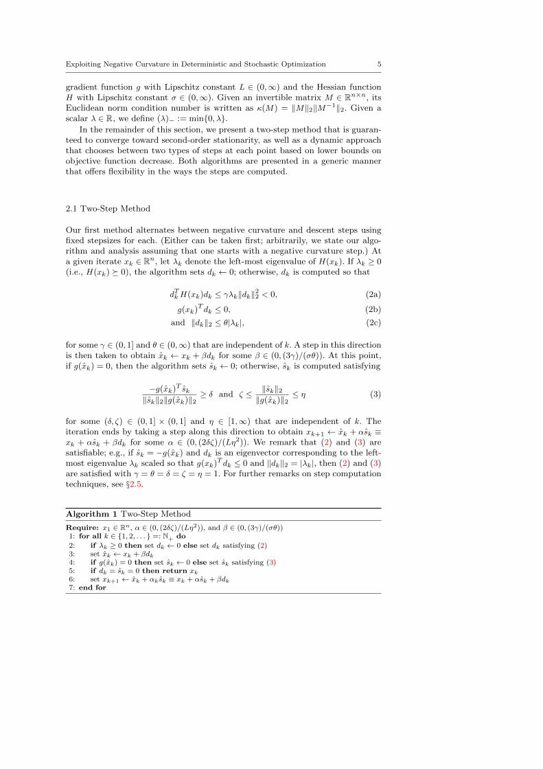
In the remainder of this section, we present a two-step method that is guaran-teed to converge toward second-order stationarity, as well as a dynamic approachthat chooses between two types of steps at each point based on lower bounds onobjective function decrease. Both algorithms are presented in a generic mannerthat offers flexibility in the ways the steps are computed.

2.1 Two-Step Method

Our first method alternates between negative curvature and descent steps usingfixed stepsizes for each. (Either can be taken first; arbitrarily, we state our algo-rithm and analysis assuming that one starts with a negative curvature step.) Ata given iterate xk ∈ Rn, let λk denote the left-most eigenvalue of H(xk). If λk ≥ 0(i.e., H(xk) � 0), the algorithm sets dk ← 0; otherwise, dk is computed so that

dTkH(xk)dk ≤ γλk‖dk‖22 < 0, (2a)

g(xk)T dk ≤ 0, (2b)

and ‖dk‖2 ≤ θ|λk|, (2c)

for some γ ∈ (0, 1] and θ ∈ (0,∞) that are independent of k. A step in this directionis then taken to obtain xk ← xk + βdk for some β ∈ (0, (3γ)/(σθ)). At this point,if g(xk) = 0, then the algorithm sets sk ← 0; otherwise, sk is computed satisfying

−g(xk)T sk‖sk‖2‖g(xk)‖2

≥ δ and ζ ≤ ‖sk‖2‖g(xk)‖2

≤ η (3)

for some (δ, ζ) ∈ (0, 1] × (0, 1] and η ∈ [1,∞) that are independent of k. Theiteration ends by taking a step along this direction to obtain xk+1 ← xk + αsk ≡xk + αsk + βdk for some α ∈ (0, (2δζ)/(Lη2)). We remark that (2) and (3) aresatisfiable; e.g., if sk = −g(xk) and dk is an eigenvector corresponding to the left-most eigenvalue λk scaled so that g(xk)T dk ≤ 0 and ‖dk‖2 = |λk|, then (2) and (3)are satisfied with γ = θ = δ = ζ = η = 1. For further remarks on step computationtechniques, see §2.5.

Algorithm 1 Two-Step Method

Require: x1 ∈ Rn, α ∈ (0, (2δζ)/(Lη2)), and β ∈ (0, (3γ)/(σθ))1: for all k ∈ {1, 2, . . . } =: N+ do

2: if λk ≥ 0 then set dk ← 0 else set dk satisfying (2)3: set xk ← xk + βdk4: if g(xk) = 0 then set sk ← 0 else set sk satisfying (3)5: if dk = sk = 0 then return xk6: set xk+1 ← xk + αk sk ≡ xk + αsk + βdk7: end for


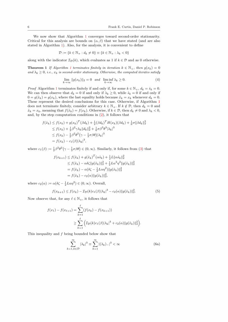
We now show that Algorithm 1 converges toward second-order stationarity.Critical for this analysis are bounds on (α, β) that we have stated (and are alsostated in Algorithm 1). Also, for the analysis, it is convenient to define

D := {k ∈ N+ : dk 6= 0} ≡ {k ∈ N+ : λk < 0}

along with the indicator ID(k), which evaluates as 1 if k ∈ D and as 0 otherwise.

Theorem 1 If Algorithm 1 terminates finitely in iteration k ∈ N+, then g(xk) = 0and λk ≥ 0, i.e., xk is second-order stationary. Otherwise, the computed iterates satisfy

limk→∞

‖g(xk)‖2 = 0 and lim infk→∞

λk ≥ 0. (4)

Proof Algorithm 1 terminates finitely if and only if, for some k ∈ N+, dk = sk = 0.We can then observe that dk = 0 if and only if λk ≥ 0, while sk = 0 if and only if0 = g(xk) = g(xk), where the last equality holds because xk = xk whenever dk = 0.These represent the desired conclusions for this case. Otherwise, if Algorithm 1does not terminate finitely, consider arbitrary k ∈ N+. If k /∈ D, then dk = 0 andxk = xk, meaning that f(xk) = f(xk). Otherwise, if k ∈ D, then dk 6= 0 and λk < 0,and, by the step computation conditions in (2), it follows that

f(xk) ≤ f(xk) + g(xk)T (βdk) + 12 (βdk)TH(xk)(βdk) + 1

6σ‖βdk‖32

≤ f(xk) + 12β

2γλk‖dk‖22 + 16σβ

3θ3|λk|3

≤ f(xk)− 12β

2θ2(γ − 13σβθ

)|λk|3

= f(xk)− c1(β)|λk|3,

where c1(β) := 12β

2θ2(γ − 1

3σβθ)∈ (0,∞). Similarly, it follows from (3) that

f(xk+1) ≤ f(xk) + g(xk)T (αsk) + 12L‖αsk‖

22

≤ f(xk)− αδζ‖g(xk)‖22 + 12Lα

2η2‖g(xk)‖22= f(xk)− α(δζ − 1

2Lαη2)‖g(xk)‖22

= f(xk)− c2(α)‖g(xk)‖22,

where c2(α) := α(δζ − 12Lαη

2) ∈ (0,∞). Overall,

f(xk+1) ≤ f(xk)− ID(k)c1(β)|λk|3 − c2(α)‖g(xk)‖22. (5)

Now observe that, for any ` ∈ N+, it follows that

f(x1)− f(x`+1) =∑k=1

(f(xk)− f(xk+1))

≥∑k=1

(ID(k)c1(β)|λk|3 + c2(α)‖g(xk)‖22

).

This inequality and f being bounded below show that

∞∑k=1,k∈D

|λk|3 ≡∞∑k=1

|(λk)−|3 <∞ (6a)


and∞∑k=1

‖g(xk)‖22 <∞. (6b)

The latter bound yields

limk→∞

‖g(xk)‖2 = 0, (7)

while the former bound and (2c) yield

∞∑k=1

‖xk − xk‖32 = β3∞∑k=1

‖dk‖32 ≤ β3θ3∞∑k=1

|(λk)−|3 <∞,

from which it follows that

limk→∞

‖xk − xk‖2 = 0. (8)

It follows from Lipschitz continuity of g along with (7) and (8) that

0 ≤ lim supk→∞

‖g(xk)‖2

= lim supk→∞

‖g(xk)− g(xk) + g(xk)‖2

≤ lim supk→∞

‖g(xk)− g(xk)‖2 + lim supk→∞

‖g(xk)‖2

≤ L lim supk→∞

‖xk − xk‖2 + lim supk→∞

‖g(xk)‖2 = 0,

which implies the first limit in (4). Finally, in order to derive a contradiction,suppose that lim infk→∞ λk < 0, meaning that there exists some ε > 0 and infiniteindex set K ⊆ D such that λk ≤ −ε for all k ∈ K. This implies that

∞∑k=1

|(λk)−|3 ≥∑k∈K|(λk)−|3 ≥

∑k∈K

ε3 =∞,

contradicting (6a). This yields the second limit in (4). ut

There are two potential weaknesses of this two-step approach. First, it sim-ply alternates back-and-forth between descent and negative curvature directions,which might not always lead to the most productive step from each point. Second,even though our analysis holds for all stepsizes α and β in the intervals providedin Algorithm 1, the algorithm might suffer from poor performance if these valuesare chosen poorly. We next present a method that addresses these weaknesses.

2.2 Dynamic Method

Suppose that, in any iteration k ∈ N+ when λk < 0, one computes a nonzerodirection of negative curvature satisfying (2a)–(2b) for some γ ∈ (0, 1]. Supposealso that, if g(xk) 6= 0, then one computes a nonzero direction sk satisfying theequivalent of the first condition in (3), namely, for some δ ∈ (0, 1],

− g(xk)T sk ≥ δ‖sk‖2‖g(xk)‖2. (9)


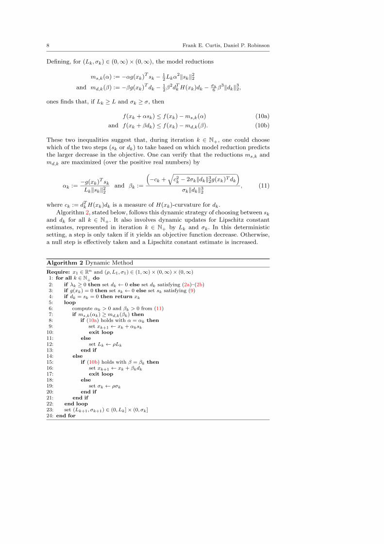
Defining, for (Lk, σk) ∈ (0,∞)× (0,∞), the model reductions

ms,k(α) := −αg(xk)T sk − 12Lkα

2‖sk‖22and md,k(β) := −βg(xk)T dk − 1

2β2dTkH(xk)dk − σk

6 β3‖dk‖32,

ones finds that, if Lk ≥ L and σk ≥ σ, then

f(xk + αsk) ≤ f(xk)−ms,k(α) (10a)

and f(xk + βdk) ≤ f(xk)−md,k(β). (10b)

These two inequalities suggest that, during iteration k ∈ N+, one could choosewhich of the two steps (sk or dk) to take based on which model reduction predictsthe larger decrease in the objective. One can verify that the reductions ms,k andmd,k are maximized (over the positive real numbers) by

αk :=−g(xk)T skLk‖sk‖22

and βk :=

(−ck +

√c2k − 2σk‖dk‖32g(xk)T dk

)σk‖dk‖32

, (11)

where ck := dTkH(xk)dk is a measure of H(xk)-curvature for dk.

Algorithm 2, stated below, follows this dynamic strategy of choosing between skand dk for all k ∈ N+. It also involves dynamic updates for Lipschitz constantestimates, represented in iteration k ∈ N+ by Lk and σk. In this deterministicsetting, a step is only taken if it yields an objective function decrease. Otherwise,a null step is effectively taken and a Lipschitz constant estimate is increased.

Algorithm 2 Dynamic Method

Require: x1 ∈ Rn and (ρ, L1, σ1) ∈ (1,∞)× (0,∞)× (0,∞)1: for all k ∈ N+ do

2: if λk ≥ 0 then set dk ← 0 else set dk satisfying (2a)–(2b)3: if g(xk) = 0 then set sk ← 0 else set sk satisfying (9)4: if dk = sk = 0 then return xk5: loop6: compute αk > 0 and βk > 0 from (11)7: if ms,k(αk) ≥ md,k(βk) then8: if (10a) holds with α = αk then9: set xk+1 ← xk + αksk

10: exit loop11: else12: set Lk ← ρLk

13: end if14: else15: if (10b) holds with β = βk then16: set xk+1 ← xk + βkdk17: exit loop18: else19: set σk ← ρσk20: end if21: end if22: end loop23: set (Lk+1, σk+1) ∈ (0, Lk]× (0, σk]24: end for


In the next two results, we establish that Algorithm 2 is well-defined and thatit has convergence guarantees on par with Algorithm 1 (recall Theorem 1).

Lemma 1 Algorithm 2 is well defined in the sense that it either terminates finitely or

generates infinitely many iterates. In addition, at the end of each iteration k ∈ N+,

Lk ≤ Lmax := max{L1, ρL} and σk ≤ σmax := max{σ1, ρσ}. (12)

Proof We begin by showing that the loop in Step 5 terminates finitely anytime itis entered. For a proof by contradiction, if that loop were never to terminate, thenthe updates to Lk and/or σk would cause at least one of them to become arbitrarilylarge. Since (10a) holds whenever Lk ≥ L and (10b) holds whenever σk ≥ σ, itfollows that the loop would eventually terminate, thus reaching a contradiction.Therefore, we have proved that the loop in Step 5 terminates finitely anytime it isentered, and moreover that (12) holds. This completes the proof once we observethat during iteration k ∈ N+, Algorithm 2 might finitely terminate in Step 4. ut

Theorem 2 If Algorithm 2 terminates finitely in iteration k ∈ N+, then g(xk) = 0and λk ≥ 0, i.e., xk is second-order stationary. Otherwise, the computed iterates satisfy

limk→∞

‖g(xk)‖2 = 0 and lim infk→∞

λk ≥ 0. (13)

Proof Algorithm 2 terminates finitely only if, for some k ∈ N+, dk = sk = 0.This can only occur if λk ≥ 0 and g(xk) = 0, which are the desired conclusions.Otherwise, Algorithm 2 does not terminate finitely and during each iteration atleast one of sk and dk is nonzero. We use this fact in the following arguments.

Consider arbitrary k ∈ N+. If sk 6= 0, then the definition of αk in (11) and thestep computation condition on sk in (9) ensure that

ms,k(αk) =1

2Lk

(g(xk)T sk‖sk‖2

)2

≥ δ2

2Lk‖g(xk)‖22. (14)

Similarly, if dk 6= 0, then by the fact that βk maximizes md,k(β) over β > 0,

(2a)–(2b), and defining βk := −2dTkH(xk)dk/(σk‖dk‖32) > 0, one finds

md,k(βk) ≥ md,k(βk)

≥ −12 β

2kdTkH(xk)dk − 1

6σkβ3k‖dk‖

32

= −2(dTkH(xk)dk)3

3σ2k‖dk‖

62

≥ 2γ3

3σ2k

|λk|3 =2γ3

3σ2k

|(λk)−|3. (15)

Overall, for all k ∈ N+, since at least one of sk and dk is nonzero, ‖gk‖2 = 0 if andonly if ‖sk‖2 = 0, and |(λk)−| = 0 if and only if ‖dk‖2 = 0, it follows that

f(xk)− f(xk+1) ≥ max

{δ2

2Lk‖g(xk)‖22,

2γ3

3σ2k

|(λk)−|3}. (16)

Indeed, to show that (16) holds, let us consider two cases. First, suppose that theupdate xk+1 ← xk+αksk is completed, meaning that (10a) holds with α = αk andms,k(αk) ≥ md,k(βk). Combining these facts with (14) and (15) establishes (16) inthis case. Second, suppose that xk+1 ← xk+βkdk is completed, meaning that (10b)


holds with β = βk and ms,k(αk) < md,k(βk). Combining these facts with (14)and (15) establishes (16) in this case. Thus, (16) holds for all k ∈ N+.

It now follows from (16), the bounds in (12), and a proof similar to that usedin Theorem 1 (in particular, to establish (6a) and (6b)) that

∞∑k=1

‖g(xk)‖22 <∞ and∞∑k=1

|(λk)−| <∞.

One may now establish the desired results in (13) using the same arguments asused in the proof of Theorem 1. ut

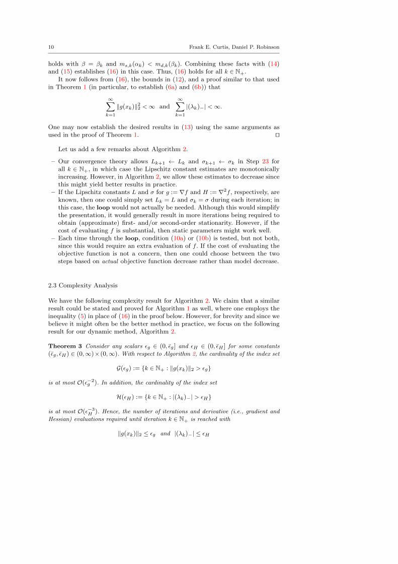
Let us add a few remarks about Algorithm 2.

– Our convergence theory allows Lk+1 ← Lk and σk+1 ← σk in Step 23 forall k ∈ N+, in which case the Lipschitz constant estimates are monotonicallyincreasing. However, in Algorithm 2, we allow these estimates to decrease sincethis might yield better results in practice.

– If the Lipschitz constants L and σ for g := ∇f and H := ∇2f , respectively, areknown, then one could simply set Lk = L and σk = σ during each iteration; inthis case, the loop would not actually be needed. Although this would simplifythe presentation, it would generally result in more iterations being required toobtain (approximate) first- and/or second-order stationarity. However, if thecost of evaluating f is substantial, then static parameters might work well.

– Each time through the loop, condition (10a) or (10b) is tested, but not both,since this would require an extra evaluation of f . If the cost of evaluating theobjective function is not a concern, then one could choose between the twosteps based on actual objective function decrease rather than model decrease.

2.3 Complexity Analysis

We have the following complexity result for Algorithm 2. We claim that a similarresult could be stated and proved for Algorithm 1 as well, where one employs theinequality (5) in place of (16) in the proof below. However, for brevity and since webelieve it might often be the better method in practice, we focus on the followingresult for our dynamic method, Algorithm 2.

Theorem 3 Consider any scalars εg ∈ (0, εg] and εH ∈ (0, εH ] for some constants

(εg, εH) ∈ (0,∞)× (0,∞). With respect to Algorithm 2, the cardinality of the index set

G(εg) := {k ∈ N+ : ‖g(xk)‖2 > εg}

is at most O(ε−2g ). In addition, the cardinality of the index set

H(εH) := {k ∈ N+ : |(λk)−| > εH}

is at most O(ε−3H ). Hence, the number of iterations and derivative (i.e., gradient and

Hessian) evaluations required until iteration k ∈ N+ is reached with

‖g(xk)‖2 ≤ εg and |(λk)−| ≤ εH


is at most O(max{ε−2g , ε−3

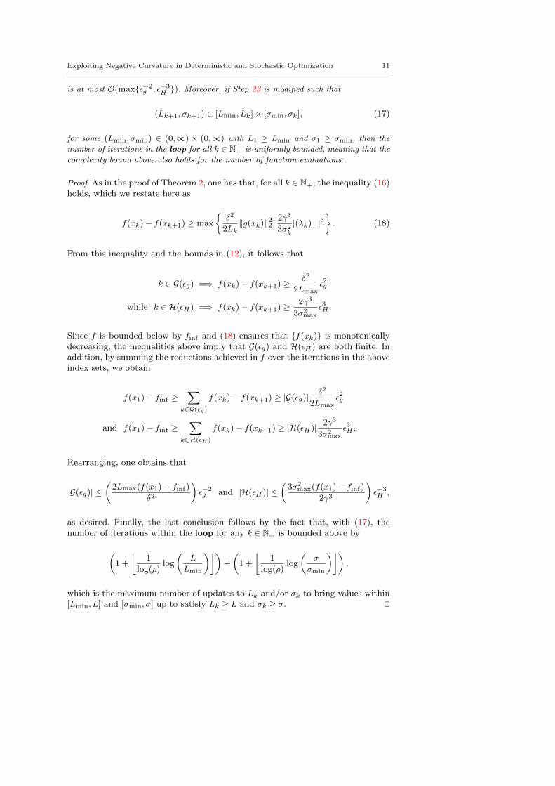
H }). Moreover, if Step 23 is modified such that

(Lk+1, σk+1) ∈ [Lmin, Lk]× [σmin, σk], (17)

for some (Lmin, σmin) ∈ (0,∞) × (0,∞) with L1 ≥ Lmin and σ1 ≥ σmin, then the

number of iterations in the loop for all k ∈ N+ is uniformly bounded, meaning that the

complexity bound above also holds for the number of function evaluations.

Proof As in the proof of Theorem 2, one has that, for all k ∈ N+, the inequality (16)holds, which we restate here as

f(xk)− f(xk+1) ≥ max

{δ2

2Lk‖g(xk)‖22,

2γ3

3σ2k

|(λk)−|3}. (18)

From this inequality and the bounds in (12), it follows that

k ∈ G(εg) =⇒ f(xk)− f(xk+1) ≥ δ2

2Lmaxε2g

while k ∈ H(εH) =⇒ f(xk)− f(xk+1) ≥ 2γ3

3σ2max

ε3H .

Since f is bounded below by finf and (18) ensures that {f(xk)} is monotonicallydecreasing, the inequalities above imply that G(εg) and H(εH) are both finite. Inaddition, by summing the reductions achieved in f over the iterations in the aboveindex sets, we obtain

f(x1)− finf ≥∑

k∈G(εg)

f(xk)− f(xk+1) ≥ |G(εg)|δ2

2Lmaxε2g

and f(x1)− finf ≥∑

k∈H(εH)

f(xk)− f(xk+1) ≥ |H(εH)| 2γ3

3σ2max

ε3H .

Rearranging, one obtains that

|G(εg)| ≤(

2Lmax(f(x1)− finf)

δ2

)ε−2g and |H(εH)| ≤

(3σ2

max(f(x1)− finf)

2γ3

)ε−3H ,

as desired. Finally, the last conclusion follows by the fact that, with (17), thenumber of iterations within the loop for any k ∈ N+ is bounded above by

(1 +

⌊1

log(ρ)log

(L

Lmin

)⌋)+

(1 +

⌊1

log(ρ)log

(σ

σmin

)⌋),

which is the maximum number of updates to Lk and/or σk to bring values within[Lmin, L] and [σmin, σ] up to satisfy Lk ≥ L and σk ≥ σ. ut


2.4 Behavior Near Strict Saddle Points

As previously mentioned (recall §1.2), much recent attention has been directedtoward the behavior of nonconvex optimization algorithms in the neighborhood ofsaddle points. In particular, in order to prove guarantees about avoiding saddlepoints, an assumption is often made about all saddle points being strict (or ridable)or even non-degenerate. Strict saddle points are those at which the Hessian has atleast one negative eigenvalue; intuitively, these are saddle points from which analgorithm should usually be expected to avoid. Nondegenerate saddle points areones at which the Hessian has no zero eigenvalues, a much stronger assumption.

One can show that in certain problems of interest, all saddle points are strict.This is interesting. However, much of the work that has discussed the behavior ofnonconvex algorithms in the neighborhood of strict saddle points have focused onstandard types of descent methods, about which one can only prove high probabil-ity results [18]. By contrast, when one considers explicitly computing directions ofnegative curvature, this is all less of an issue. After all, notice that our convergenceand complexity analyses for our framework did not require careful considerationof the nature of any potential saddle points.

In any case, for ease of comparison to other recent analyses, let us discussthe convergence/complexity properties for our method in the context of a strictsaddle point assumption. Suppose that the set of maximizers and saddle pointsof f , say {xi}i∈I for some index set I, which must necessarily have g(xi) = 0 forall i ∈ I, also has λi < 0 for all i ∈ I, where {λi}i∈I are the leftmost eigenvaluesof {H(xi)}i∈I and are uniformly bounded away from zero. In this setting, we maydraw the following conclusions from Theorems 2 and 3.

– Any limit point of the sequence {xk} computed by Algorithm 2 is a minimizerof f . This follows since Theorem 2 ensures that for any limit point, say x,the gradient must be zero and the leftmost eigenvalue must be nonnegative.It follows from these facts and the assumptions on the maximizers and saddlepoints {xi} that x must be a minimizer, as claimed.

– From the discussion in the previous bullet and Theorem 3 we know, in fact, thatthe iterates of Algorithm 2 must eventually enter a region consisting only ofminimizers (i.e., one that does not contain any maximizers or saddle points) ina number of iterations that is polynomial in ε ∈ (0,∞), where the negative value−ε is greater than the largest of the leftmost eigenvalues of {H(xi)}i∈I . Thiscomplexity result holds without assuming that the minimizers, maximizers, andsaddle points are all nondegenerate (i.e., the Hessian matrix at these pointsare nonsingular), which, e.g., should be contrasted with the analysis in [26, seeAssumption 3]. The primary reason for our stronger convergence/complexityproperties is that our method incorporates negative curvature directions whenthey exist, as opposed to only descent directions.

2.5 Step Computation Techniques

There is flexibility in the ways in which the steps dk and sk (or sk) are computedin order to satisfy the desired conditions (in (2) and (3)/(9)). For example, skmight be the steepest descent direction −g(xk), for which (3) holds with δ =ζ = η = 1. Another option, with a symmetric positive definite B−1

k ∈ Rn×n


that has κ(B−1k ) ≤ δ−1 with a spectrum falling in [ζ, η], is to compute sk as the

modified Newton direction −B−1k g(xk). A particularly attractive option for certain

applications (when Hessian-vector products are readily computed) is to compute skvia a Newton-CG routine [25] with safeguards that terminate the iteration beforea CG iterate is computed that violates (3) for prescribed (δ, ζ, η).

There are multiple ways to compute the negative curvature direction. In theory,the most straightforward approach is to set dk = ±vk, where vk is a leftmost eigen-vector of H(xk). With this choice, it follows that dTkH(xk)dk = λk‖dk‖2, meaningthat (2a) is satisfied, and one can scale dk to ensure that (2b) and (2c) hold. Asecond approach for large-scale settings (i.e., when n is large) is to compute dk viamatrix-free Lanczos iterations [16]. Such an approach can produce a direction dksatisfying (2a), which can then be scaled to yield (2b) and (2c).

2.6 Numerical Results

In this section, we demonstrate that there can be practical benefits of following di-rections of negative curvature if one follows the dynamic approach of Algorithm 2.To do this, we implemented software in Matlab that, for all k ∈ N+, has theoption to compute sk via several options (see §2.6.1 and §2.6.2) and dk = ±vk(recall §2.5). Our test problems include a subset of the CUTEst collection [12].Specifically, we selected all of the unconstrained problems with n ≤ 500 and secondderivatives explicitly available. This left us with a test set of 97 problems.

Using this test set, we considered two variants of Algorithm 2: (i) a version inwhich the if condition in Step 7 is always presumed to test true, i.e., the descentstep sk is chosen for all k ∈ N+ (which we refer to as Algorithm 2(sk)), and(ii) a version that, as in our formal statement of the algorithm, chooses betweendescent and negative curvature steps by comparing model reduction values foreach k ∈ N+ (which we refer to as Algorithm 2(sk, dk)). In our experiments, weused L1 ← 1 and σ1 ← 1, updating them and setting subsequent values in theirrespective sequences using the following strategy. For increasing one of these valuesin Step 12 or Step 19, we respectively set the quantities

Lk ← Lk +2(f(xk + αksk)− f(xk) +ms,k(αk)

)α2k‖sk‖2

or

σk ← σk +6(f(xk + βkdk)− f(xk) +md,k(βk)

)β3k‖dk‖3

,

then, with ρ← 2, use the update

Lk ← max{ρLk,min{103Lk, Lk}} in Step 12 of Algorithm 2 or

σk ← max{ρσk,min{103σk, σk}} in Step 19 of Algorithm 2.(19)

The quantity Lk is defined so that (10a) holds at equality with α = αk and Lkreplaced by Lk in the definition of ms,k(αk), i.e., Lk is the value that makes themodel decrease agree with the exact function decrease at xk+αksk. The procedurewe use to set σk is analogous. We remark that the updates in (19) ensure thatLk ∈ [ρLk, 103Lk] and σk ∈ [ρσk, 103σk], which we claim maintains the convergenceand complexity guarantees of Algorithm 2. Moreover, when Step 12 (respectively,


Step 19) is reached, then it must be the case that Lk > Lk (respectively, σk > σk).On the other hand, in Step 23 we use the following updates:

Lk+1 ← max{10−3, 10−3Lk, Lk} and σk+1 ← σk when xk+1 ← xk + αksk;

σk+1 ← max{10−3, 10−3σk, σk} and Lk+1 ← Lk when xk+1 ← xk + βkdk.

Over the next two sections, we discuss numerical results when two different optionsfor computing the descent direction sk are used.

2.6.1 Choosing sk as the direction of steepest descent

The tests in this section use the steepest descent direction, i.e., sk = −g(xk) for allk ∈ N+. Although this is a simple choice, it gives a starting point for understandingthe potential benefits of using directions of negative curvature.

We ran Algorithm 2(sk) and Algorithm 2(sk, dk) on the previously describedCUTEst problems with commonly used stopping conditions. Specifically, an algo-rithm terminates with an approximate second-order stationary solution if

‖g(xk)‖ ≤ 10−5 max{1, ‖g(x1)‖} and |(λk)−| ≤ 10−5 max{1, |(λ1)−|}. (20)

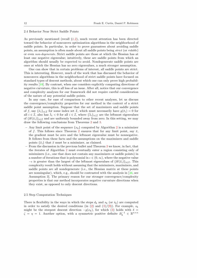
We also terminate an algorithm if an iteration limit of 10,000 is reached or if atrial step smaller than 10−16 is computed. The results can be found in Figure 1.

In Figure 1a, letting ffinal(sk) and ffinal(sk, dk) be the final computed objectivevalues for Algorithm 2(sk) and Algorithm 2(sk, dk), respectively, we plot

ffinal(sk)− ffinal(sk, dk)

max{|ffinal(sk)|, |ffinal(sk, dk)|, 1}∈ [−2, 2] (21)

for each problem that Algorithm 2(sk, dk) used at least one negative curvature di-rection. In this manner, an upward pointing bar implies that Algorithm 2(sk, dk)terminated with a lower value of the objective function, while its magnitude repre-sents how much better was this value. We can observe from Figure 1a that amongthe 39 problems, Algorithm 2(sk) terminated with a significantly lower objectivevalue compared to Algorithm 2(sk, dk) only 2 times. (While the value in (21) fallsin the interval [−2, 2], the bars in the figure all fall within [−1, 1] since, for eachproblem, the final function value reached by each algorithm had the same sign.)

We are also interested in the number of iterations and objective function eval-uations needed to obtain these final objective function values. The relative perfor-mances of the algorithms with respect to these measures are shown in Figure 1band Figure 1c. In particular, letting #its(sk) be the total number of iterationsrequired by Algorithm 2(sk) and #its(sk, dk) be the total number of iterationsrequired by Algorithm 2(sk, dk), we plot in Figure 1b the values

#its(sk)−#its(sk, dk)

max{#its(sk),#its(sk, dk), 1}∈ [−1, 1], (22)

and, letting #fevals(sk) be the total number of objective function evaluations forAlgorithm 2(sk) and #fevals(sk, dk) be the total number of objective functionevaluations for Algorithm 2(sk, dk), we plot in Figure 1c the values

#fevals(sk)−#fevals(sk, dk)

max{#fevals(sk),#fevals(sk, dk), 1}∈ [−1, 1]. (23)


0 5 10 15 20 25 30 35-1

-0.8

-0.6

-0.4

-0.2

0

0.2

0.4

0.6

0.8

1

RA

T43

LSV

IBR

BE

AM

RA

T42

LSM

ISR

A1A

LSG

RO

WT

HLS

HE

AR

T6L

ST

HU

RB

ER

LSM

EY

ER

3V

ES

UV

IALS

NE

LSO

NLS

MG

H09

LSB

IGG

S6

HIM

ME

LBF

GU

LFLA

NC

ZO

S2L

SLA

NC

ZO

S3L

SLA

NC

ZO

S1L

SH

ELI

XM

AR

AT

OS

BC

UB

EH

AT

FLD

DH

UM

PS

RO

SE

NB

RD

EN

SC

HN

EK

OW

OS

BS

INE

VA

LA

LLIN

ITU

DJT

LE

NS

OLS

HA

IRY

LOG

HA

IRY

SN

AIL

OS

BO

RN

EB

HE

AR

T8L

SE

NG

VA

L2C

HW

IRU

T2L

SM

GH

17LS

KIR

BY

2LS

HY

DC

20LS

(a) Plot associated with the quantity (21).

0 5 10 15 20 25 30 35-1

-0.8

-0.6

-0.4

-0.2

0

0.2

0.4

0.6

0.8

1

RA

T43

LSV

IBR

BE

AM

RA

T42

LSM

ISR

A1A

LSG

RO

WT

HLS

HE

AR

T6L

ST

HU

RB

ER

LSM

EY

ER

3V

ES

UV

IALS

NE

LSO

NLS

MG

H09

LSB

IGG

S6

HIM

ME

LBF

GU

LFLA

NC

ZO

S2L

SLA

NC

ZO

S3L

SLA

NC

ZO

S1L

SH

ELI

XM

AR

AT

OS

BC

UB

EH

AT

FLD

DH

UM

PS

RO

SE

NB

RD

EN

SC

HN

EK

OW

OS

BS

INE

VA

LA

LLIN

ITU

DJT

LE

NS

OLS

HA

IRY

LOG

HA

IRY

SN

AIL

OS

BO

RN

EB

HE

AR

T8L

SE

NG

VA

L2C

HW

IRU

T2L

SM

GH

17LS

KIR

BY

2LS

HY

DC

20LS

(b) Plot associated with the quantity (22).

0 5 10 15 20 25 30 35-1

-0.8

-0.6

-0.4

-0.2

0

0.2

0.4

0.6

0.8

1

RA

T43

LSV

IBR

BE

AM

RA

T42

LSM

ISR

A1A

LSG

RO

WT

HLS

HE

AR

T6L

ST

HU

RB

ER

LSM

EY

ER

3V

ES

UV

IALS

NE

LSO

NLS

MG

H09

LSB

IGG

S6

HIM

ME

LBF

GU

LFLA

NC

ZO

S2L

SLA

NC

ZO

S3L

SLA

NC

ZO

S1L

SH

ELI

XM

AR

AT

OS

BC

UB

EH

AT

FLD

DH

UM

PS

RO

SE

NB

RD

EN

SC

HN

EK

OW

OS

BS

INE

VA

LA

LLIN

ITU

DJT

LE

NS

OLS

HA

IRY

LOG

HA

IRY

SN

AIL

OS

BO

RN

EB

HE

AR

T8L

SE

NG

VA

L2C

HW

IRU

T2L

SM

GH

17LS

KIR

BY

2LS

HY

DC

20LS

(c) Plot associated with the quantity (23).

Fig. 1: Plots for the choice sk ≡ −g(xk) for all k ∈ N+. Only problems for whichat least one negative curvature direction is used are presented. The problems areordered based on the values in plot (a).

These two plots show that Algorithm 2(sk, dk) tends to perform better than Al-gorithm 2(sk) in terms of both the number of required iterations and functionevaluations. Overall, we find these results interesting since Algorithm 2(sk, dk)tends to find lower values of the objective function (see Figure 1a) while typicallyrequiring fewer iterations (see Figure 1b) and function evaluations (see Figure 1c).

2.6.2 Choosing sk using a modified-Newton strategy

In this subsection, we show the results of tests similar to those in §2.6.1 exceptthat now we compute the descent direction sk by a modified-Newton approach.Specifically, we compute sk as the unique vector satisfying Bksk = −g(xk) with

Bk = H(xk) + δkI, (24)

where I is the identify matrix and δk is the smallest nonnegative real number suchthat Bk is positive definite with a condition number less than or equal to 108.


0 5 10 15 20 25 30 35 40 45-1

-0.8

-0.6

-0.4

-0.2

0

0.2

0.4

0.6

0.8

1

HE

AR

T8L

SO

SB

OR

NE

BLO

GH

AIR

YE

CK

ER

LE4L

SM

ISR

A1A

LSD

EN

SC

HN

DH

EA

RT

6LS

BIG

GS

6R

OS

ZM

AN

1LS

NE

LSO

NLS

HA

HN

1LS

BE

NN

ET

T5L

SM

EY

ER

3M

GH

10LS

OS

BO

RN

EA

GR

OW

TH

LSLA

NC

ZO

S3L

SH

UM

PS

LAN

CZ

OS

2LS

DE

NS

CH

NE

DA

NW

OO

DLS

EN

GV

AL2

BE

ALE

ALL

INIT

UD

JTL

EN

SO

LSE

XP

FIT

HA

IRY

KO

WO

SB

RA

T43

LSS

INE

VA

LS

NA

ILH

AT

FLD

EH

AT

FLD

DR

AT

42LS

DE

CO

NV

UG

ULF

HE

LIX

LAN

CZ

OS

1LS

MG

H09

LSP

OW

ELL

BS

LSM

GH

17LS

TH

UR

BE

RLS

CH

WIR

UT

1LS

CH

WIR

UT

2LS

HY

DC

20LS

VIB

RB

EA

MK

IRB

Y2L

S

(a) Plot associated with the quantity (21).

0 5 10 15 20 25 30 35 40 45-1

-0.8

-0.6

-0.4

-0.2

0

0.2

0.4

0.6

0.8

1

HE

AR

T8L

SO

SB

OR

NE

BLO

GH

AIR

YE

CK

ER

LE4L

SM

ISR

A1A

LSD

EN

SC

HN

DH

EA

RT

6LS

BIG

GS

6R

OS

ZM

AN

1LS

NE

LSO

NLS

HA

HN

1LS

BE

NN

ET

T5L

SM

EY

ER

3M

GH

10LS

OS

BO

RN

EA

GR

OW

TH

LSLA

NC

ZO

S3L

SH

UM

PS

LAN

CZ

OS

2LS

DE

NS

CH

NE

DA

NW

OO

DLS

EN

GV

AL2

BE

ALE

ALL

INIT

UD

JTL

EN

SO

LSE

XP

FIT

HA

IRY

KO

WO

SB

RA

T43

LSS

INE

VA

LS

NA

ILH

AT

FLD

EH

AT

FLD

DR

AT

42LS

DE

CO

NV

UG

ULF

HE

LIX

LAN

CZ

OS

1LS

MG

H09

LSP

OW

ELL

BS

LSM

GH

17LS

TH

UR

BE

RLS

CH

WIR

UT

1LS

CH

WIR

UT

2LS

HY

DC

20LS

VIB

RB

EA

MK

IRB

Y2L

S

(b) Plot associated with the quantity (22).

0 5 10 15 20 25 30 35 40 45-1

-0.8

-0.6

-0.4

-0.2

0

0.2

0.4

0.6

0.8

1

HE

AR

T8L

SO

SB

OR

NE

BLO

GH

AIR

YE

CK

ER

LE4L

SM

ISR

A1A

LSD

EN

SC

HN

DH

EA

RT

6LS

BIG

GS

6R

OS

ZM

AN

1LS

NE

LSO

NLS

HA

HN

1LS

BE

NN

ET

T5L

SM

EY

ER

3M

GH

10LS

OS

BO

RN

EA

GR

OW

TH

LSLA

NC

ZO

S3L

SH

UM

PS

LAN

CZ

OS

2LS

DE

NS

CH

NE

DA

NW

OO

DLS

EN

GV

AL2

BE

ALE

ALL

INIT

UD

JTL

EN

SO

LSE

XP

FIT

HA

IRY

KO

WO

SB

RA

T43

LSS

INE

VA

LS

NA

ILH

AT

FLD

EH

AT

FLD

DR

AT

42LS

DE

CO

NV

UG

ULF

HE

LIX

LAN

CZ

OS

1LS

MG

H09

LSP

OW

ELL

BS

LSM

GH

17LS

TH

UR

BE

RLS

CH

WIR

UT

1LS

CH

WIR

UT

2LS

HY

DC

20LS

VIB

RB

EA

MK

IRB

Y2L

S

(c) Plot associated with the quantity (23).

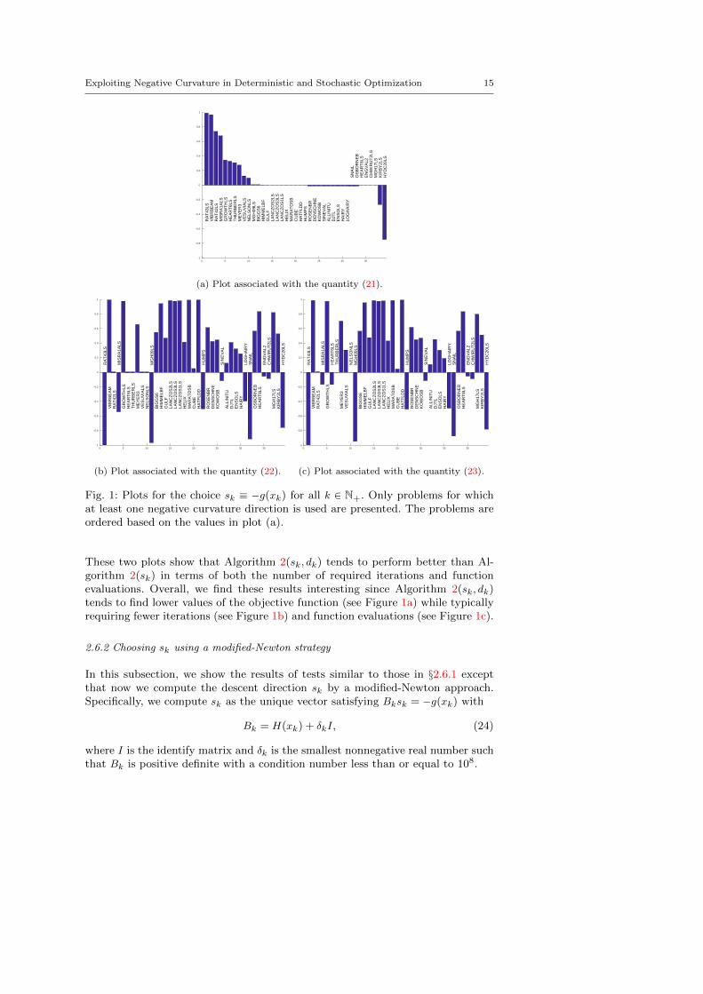
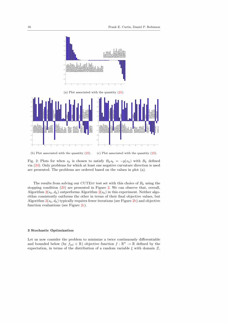
Fig. 2: Plots for when sk is chosen to satisfy Bksk = −g(xk) with Bk definedvia (24). Only problems for which at least one negative curvature direction is usedare presented. The problems are ordered based on the values in plot (a).

The results from solving our CUTEst test set with this choice of Bk using thestopping condition (20) are presented in Figure 2. We can observe that, overall,Algorithm 2(sk, dk) outperforms Algorithm 2(sk) in this experiment. Neither algo-rithm consistently outforms the other in terms of their final objective values, butAlgorithm 2(sk, dk) typically requires fewer iterations (see Figure 2b) and objectivefunction evaluations (see Figure 2c).

3 Stochastic Optimization

Let us now consider the problem to minimize a twice continuously differentiableand bounded below (by finf ∈ R) objective function f : Rn → R defined by theexpectation, in terms of the distribution of a random variable ξ with domain Ξ,


of a stochastic function F : Rn × Ξ → R, namely,

minx∈Rn

f(x), where f(x) := Eξ[F (x, ξ)]. (25)

In this context, we expect that, at an iterate xk, one can only compute stochas-tic gradient and Hessian estimates. We do not claim that we are able to proveconvergence guarantees to second-order stationarity as in the deterministic case.That said, we are able to present a two-step method with convergence guaranteesto first-order stationarity whose structure motivates a dynamic method that weshow can offer beneficial practical performance by exploring negative curvature.

3.1 Two-Step Method: Stochastic Gradient/Newton with “Curvature Noise”

At an iterate xk, let ξk be a random variable representing a seed for generating avector sk ∈ Rn. For example, if f is the expected function value over inputs from adataset, then ξk might represent sets of points randomly drawn from the dataset.With Eξk [·] denoting expectation taken with respect to the distribution of ξk giventhe current iterate xk, we require the vector sk to satisfy

−∇f(xk)TEξk [sk] ≥ δ‖∇f(xk)‖22, (26a)

Eξk [‖sk‖2] ≤ η‖∇f(xk)‖2, and (26b)

Eξk [‖sk‖22] ≤Ms1 +Ms2‖∇f(xk)‖22 (26c)

for some δ ∈ (0, 1], η ∈ [1,∞), and (Ms1,Ms2) ∈ (0,∞) × (1,∞) that are allindependent of k. For example, as in a stochastic gradient method, these conditionsare satisfied if sk is an unbiased estimate of ∇f(xk) with second moment boundedas in (26c). They are also satisfied in the context of a stochastic Newton methodwherein a stochastic gradient estimate is multiplied by a stochastic inverse Hessianestimate, assuming that the latter is conditionally uncorrelated with the formerand has eigenvalues contained within an interval of the positive real line uniformlyover all k ∈ N+.

Let us also define ξHk , conditionally uncorrelated with ξk given xk, as a randomvariable representing a seed for generating an unbiased Hessian estimate Hk suchthat EξHk [Hk] = ∇2f(xk). We use Hk to compute a direction dk. For the purpose

of ideally following a direction of negative curvature (for the true Hessian), we askthat dk satisfies a curvature condition similar to that used in the deterministicsetting. Importantly, however, the second moment of dk must be bounded similarto that of sk above. Overall, with λk being the left-most eigenvalue of Hk, we setdk ← 0 if λk ≥ 0, and otherwise require the direction dk to satisfy

dTkHkdk ≤ γλk‖dk‖22 < 0 given Hk (27a)

and EξHk [‖dk‖22] ≤Md1 +Md2‖∇f(xk)‖22 (27b)

for some γ ∈ (0, 1] and (Md1,Md2) ∈ (0,∞) × (1,∞) that are independent of k.One manner in which these conditions can be satisfied is to compute dk as aneigenvector corresponding to the left-most eigenvalue λk, scaled such that ‖dk‖22is bounded above in proportion to the squared norm ‖sk‖22 where sk satisfies (26).


Note that our conditions in (27) do not involve expected descent with respect tothe true gradient at xk. This can be viewed in contrast to (2), which involves (2b).The reason for this is that, in a practical setting, such a condition might notbe verifiable without computing the exact gradient explicitly, which might beintractable or prohibitively expensive. Instead, without this restriction, a criticalcomponent of our algorithm is the generation of an independent random scalar ωkuniformly distributed in [−1, 1]. With this choice, one finds E(ξHk ,ωk)[ωkdk] = 0 such

that, effectively, ωkdk merely adds noise to sk in a manner that ideally follows anegative curvature direction. This leads to Algorithm 3 below.

Algorithm 3 Two-Step Method for Stochastic Optimization

Require: x1 ∈ Rn, {αk} ⊂ (0,∞), and {βk} ⊂ (0,∞)1: for all k ∈ N+ do

2: generate uncorrelated random seeds ξk and ξHk3: generate ωk uniformly in [−1, 1]4: set sk satisfying (26)5: set dk satisfying (27)6: set xk+1 ← xk + αksk + βkωkdk7: end for

Algorithm 3 maintains the convergence guarantees of a standard stochasticgradient (SG) method. To show this, let us first prove the following lemma.

Lemma 2 For all k ∈ N+, it follows that

E(ξk,ξHk ,ωk)[f(xk+1)]− f(xk)

≤ − (δαk − 12LMs2α

2k − 1

6LMd2β2k)‖∇f(xk)‖22 + 1

2LMs1α2k + 1

6LMd1β2k .

(28)

Proof From Lipschitz continuity of ∇f , it follows that

f(xk+1)− f(xk) = f(xk + αksk + βkωkdk)− f(xk)

≤ ∇f(xk)T (αksk + βkωkdk) + 12L‖αksk + βkωkdk‖22.

Taking expectations with respect to the distribution of the random quantities(ξk, ξ

Hk , ωk) given xk and using (26)–(27), it follows that

E(ξk,ξHk ,ωk)[f(xk+1)]− f(xk)

≤ ∇f(xk)T (αkEξk [sk] + βkE(ξHk ,ωk)[ωkdk])

+ 12L(α2

kEξk [‖sk‖22] + β2kE(ξHk ,ωk)[‖ωkdk‖

22])

+ LαkβkE(ξk,ξHk ,ωk)[sTk (ωkdk)]

≤ − αkδ‖∇f(xk)‖22+ 1

2Lα2k(Ms1 +Ms2‖∇f(xk)‖22) + 1

6Lβ2k(Md1 +Md2‖∇f(xk)‖22).

Rearranging, we reach the desired conclusion. ut


From this lemma, we obtain a critical bound similar to one that can be shownfor a generic SG method; e.g., see Lemma 4.4 in [2]. Hence, following analyses suchas that in [2], one can show that the total expectation for the gap between f(xk)and a lower bound for f decreases. For instance, we prove the following theoremusing similar proof techniques as for Theorems 4.8 and 4.9 in [2].

Theorem 4 Suppose that Algorithm 3 is run with αk = βk = α for all k ∈ N+ where

0 < α ≤ δ

2Lmax{Ms2,Md2}. (29)

Then, for all K ∈ N+, one has that

E

[1

K

K∑k=1

‖∇f(xk)‖22

]≤ 2αLmax{Ms1,Md1}

δ+

2(f(x1)− finf)

Kδα

K→∞−−−−→ 2αLmax{Ms1,Md1}

δ.

On the other hand, if Algorithm 3 is run with {αk} satisfying

∞∑k=1

αk =∞ and

∞∑k=1

α2k <∞ (30)

and {βk} = {χαk} for some χ ∈ (0,∞), then it holds that

limK→∞

E

[K∑k=1

αk‖∇f(xk)‖22

]<∞,

from which it follows, with AK :=∑Kk=1 αk, that

limK→∞

E

[1

AK

K∑k=1

αk‖∇f(xk)‖22

]= 0,

which implies that lim infk→∞ E[‖∇f(xk)‖22] = 0.

Proof First, suppose that Algorithm 3 is run with αk = βk = α for all k ∈ N+.Then, taking total expectation in (28), it follows with (29) and since 1

2 >16 that

E[f(xk+1)]− E[f(xk)]

≤ − (δ − Lmax{Ms2,Md2}α)αE[‖∇f(xk)‖22] + Lmax{Ms1,Md1}α2

≤ − 12δαE[‖∇f(xk)‖22] + Lmax{Ms1,Md1}α2.

Summing both sides of this inequality for k ∈ {1, . . . ,K} yields

finf − f(x1) ≤ E[f(xK+1)]− f(x1)

≤ −12δα

K∑k=1

E[‖∇f(xk)‖22] +KLmax{Ms1,Md1}α2.

Rearranging and dividing further by K yields the desired conclusion.


Now suppose that Algorithm 3 is run with {αk} and {βk} = {χαk} such thatthe former satisfies (30). Since the second condition in (30) ensures that {αk} ↘ 0,we may assume without loss of generality that, for all k ∈ N+,

αk ≤ min

{δ

2LMs2,

3δ

2LMd2χ2

}.

Thus, taking total expectation in (28) leads to

E[f(xk+1)]− E[f(xk)]

≤ − (δαk − 12LMs2α

2k − 1

6LMd2β2k)E[‖∇f(xk)‖22] + 1

2LMs1α2k + 1

6LMd1β2k

≤ − 12δαkE[‖∇f(xk)‖22] + (1

2LMs1 + 16LMd1χ

2)α2k.

Summing both sides for k ∈ {1, . . . ,K} yields

finf − f(x1) ≤ E[f(xK+1)]− f(x1)

≤ −12δ

K∑k=1

αkE[‖∇f(xk)‖22] + (12LMs1 + 1

6LMd1χ2)

K∑k=1

α2k,

from which it follows that

K∑k=1

αkE[‖∇f(xk)‖22] ≤ 2(f(x1)− finf)

δ+LMs1 + 1

3LMd1χ2

δ

K∑k=1

α2k.

The second of the conditions in (30) implies that the right-hand side here convergesto a finite limit when K →∞. Then, the rest of the desired conclusion follows sincethe first of the conditions in (30) ensures that AK →∞ as K →∞. ut

3.2 Dynamic Method

Borrowing ideas from the two-step deterministic method in §2.1, the dynamic de-terministic method in §2.2, and the two-step stochastic method in §3.1, we proposethe dynamic method for stochastic optimization presented as Algorithm 4 below.After computing a stochastic Hessian estimate Hk ∈ Rn×n and an independentstochastic gradient estimate gk ∈ Rn, the algorithm employs the conjugate gradi-ent (CG) method [25] for solving the linear system Hks = −gk with the startingpoint s ← 0. If Hk � 0, then it is well known that this method solves this sys-tem in at most n iterations (in exact arithmetic). However, if Hk 6� 0, then themethod might encounter a direction of nonpositive curvature, say p ∈ Rn, suchthat pTHkp ≤ 0. If this occurs, then we terminate CG immediately and set dk ← p.This choice is made rather than spend any extra computational effort attemptingto approximate an eigenvector corresponding to the left-most eigenvalue of Hk.Otherwise, if no such direction of nonpositive curvature is encountered, then thealgorithm chooses dk ← 0. In either case, the algorithm sets sk as the final CGiterate computed prior to termination. (The only special case is when nonpositivecurvature is encountered in the first iteration; then, sk ← −gk and dk ← 0.)

For setting values for the dynamic parameters {Lk} and {σk}, which in turndetermine the stepsize sequences {αk} and {βk}, the algorithm employs stochastic


function value estimates. In this manner, the algorithm can avoid computing theexact objective value at any point (which is often not tractable). In the statementof the algorithm, we use fk : Rn → R to indicate a function that yields a stochasticfunction estimate during iteration k ∈ N+.

Algorithm 4 Dynamic Method for Stochastic Optimization

Require: x1 ∈ Rn and (L1, σ1) ∈ (0,∞)× (0,∞)1: for all k ∈ N+ do2: generate a stochastic gradient gk and stochastic Hessian Hk

3: run CG on Hks = −gk to compute sk and dk (as described in the text above)4: set αk ← 1/Lk and βk ← 1/σk5: set xk ← xk + αksk6: if fk(xk) > fk(xk) then7: set Lk+1 ∈ [Lk,∞)8: (optional) reset xk ← xk9: else

10: set Lk+1 ∈ (0, Lk]11: end if12: set xk+1 ← xk + βkdk13: if fk(xk+1) > fk(xk) then14: set σk+1 ∈ [σk,∞)15: (optional) reset xk+1 ← xk16: else17: set σk+1 ∈ (0, σk]18: end if19: end for

As previously mentioned, we do not claim convergence guarantees for thismethod. However, we believe that it is well motivated by our previous algorithms.One should also note that the per-iteration cost between this method and an inex-act Newton-CG method is negligible since any computed dk 6= 0 comes essentiallyfor free from the CG routine. The only significant extra cost might come fromthe stochastic function estimates, though these can be made cheaper than anystochastic gradient estimate and might even be ignored completely if one is ableto tune fixed values for L and σ that work well for a particular application.

3.3 Numerical Experiments

We implemented Algorithm 4 in Python 2.7.13. As a test problem, we trained aconvolutional neural network to classify handwritten digits in the well-known mnist

dataset; see [17]. Our neural network, implemented using tensorflow,1 is composedof two convolutional layers followed by a fully connected layer. In each iteration, wecomputed stochastic gradient and Hessian estimates using independently drawnmini-batches of size 500. By contrast, the entire training dataset involves 60,000feature/label pairs. The testing set involves 10,000 feature/label pairs.

In each iteration, our implementation runs the CG method for at most 10 it-erations. If a direction of nonpositive curvature is found within this number ofiterations, then it is employed as dk; otherwise, dk ← 0. In preliminary training

1 https://www.tensorflow.org/

https://www.tensorflow.org/


runs, we occasionally witnessed instances in which a particularly large stochasticgradient led to a large step, which in turn spoiled all previous progress made bythe algorithm. Hence, to control the iterate displacements, we scaled sk and/or dkdown, when necessary, to ensure that ‖sk‖ ≤ 10 and ‖βkdk‖ ≤ 0.2‖αksk‖. We wit-nessed similar poor behavior when the Lipschitz constant estimates were initializedto be too small; hence, for our experiments, we chose L1 ← 80 and σ1 ← 100 asthe smallest values that yielded stable algorithm behavior for both algorithms. Ifstochastic function evaluations suggested an objective increase, then an estimatewas increased by a factor of 1.2; see Steps 7 and 14 in Algorithm 4. The imple-mentation never decreases these estimates. In addition, while the implementationalways takes the step αksk (i.e., it does not follow the optional Step 8), it doesreset xk+1 ← xk (recall Step 15) if/when the stochastic function estimates predictan increase in f due to the step βkdk.

For comparison purposes, we ran the algorithm twice using the same startingpoint and initial seeds for the random number generators: once with βk being resetto zero for all k ∈ N+ (so that no step along dk is ever taken) and once with it setas in Algorithm 4. We refer to the former algorithm as SG since it is a stochastic-gradient-type method that does not explore negative curvature. We refer to thelatter as NC since it attempts to exploit negative curvature.

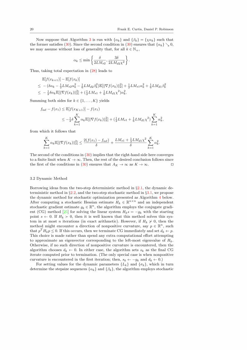
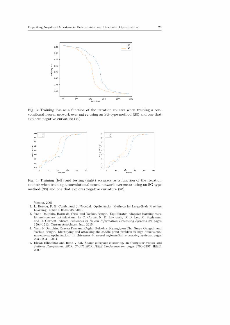
The training losses as a function of the iteration counter are shown in Figure 3.As can be seen in the plot, the performance of the two algorithms is initially verysimilar. However, after some initial iterations, following the negative curvaturesteps consistently offers additional progress, allowing NC to reduce the loss andincrease both the training and testing accuracy more rapidly than SG. Eventually,the plots in each of the figures near each other (after around two epochs, whenthe algorithms were terminated). This should be expected as both algorithmseventually near stationary points. However, prior to this point, NC has successfullyavoided the early stagnation experienced by SG.

4 Conclusion

We have confronted the question of whether it can be beneficial for nonconvex op-timization algorithms to compute and explore directions of negative curvature. Wehave proposed new algorithmic frameworks based on the idea that an algorithmmight alternate or choose between descent and negative curvature steps based onproperties of upper-bounding models of the objective function. In the case of de-terministic optimization, we have shown that our frameworks possess convergenceand competitive complexity guarantees in the pursuit of first- and second-orderstationary points, and have demonstrated that instances of our framework out-perform descent-step-only methods in terms of finding points with lower objectivevalues typically within fewer iterations and function evaluations. In the case ofstochastic optimization, we have shown that an algorithm that employs “curva-ture noise” can outperform a stochastic-gradient-based approach.

References

1. E. G. Birgin and J. M. Martınez. A Box-Constrained Optimization Algorithm with Nega-tive Curvature Directions and Spectral Projected Gradients, pages 49–60. Springer Vienna,


Fig. 3: Training loss as a function of the iteration counter when training a con-volutional neural network over mnist using an SG-type method (SG) and one thatexplores negative curvature (NC).

Fig. 4: Training (left) and testing (right) accuracy as a function of the iterationcounter when training a convolutional neural network over mnist using an SG-typemethod (SG) and one that explores negative curvature (NC).

Vienna, 2001.2. L. Bottou, F. E. Curtis, and J. Nocedal. Optimization Methods for Large-Scale Machine

Learning. arXiv 1606.04838, 2016.3. Yann Dauphin, Harm de Vries, and Yoshua Bengio. Equilibrated adaptive learning rates

for non-convex optimization. In C. Cortes, N. D. Lawrence, D. D. Lee, M. Sugiyama,and R. Garnett, editors, Advances in Neural Information Processing Systems 28, pages1504–1512. Curran Associates, Inc., 2015.

4. Yann N Dauphin, Razvan Pascanu, Caglar Gulcehre, Kyunghyun Cho, Surya Ganguli, andYoshua Bengio. Identifying and attacking the saddle point problem in high-dimensionalnon-convex optimization. In Advances in neural information processing systems, pages2933–2941, 2014.

5. Ehsan Elhamifar and Rene Vidal. Sparse subspace clustering. In Computer Vision andPattern Recognition, 2009. CVPR 2009. IEEE Conference on, pages 2790–2797. IEEE,2009.


6. Anders Forsgren, Philip E Gill, and Walter Murray. Computing modified newton directionsusing a partial cholesky factorization. SIAM Journal on Scientific Computing, 16(1):139–150, 1995.

7. R. Ge, F. Huang, C. Jin, and Y. Yuan. Escaping From Saddle Points — Online StochasticGradient for Tensor Decomposition. In JMLR: Workshop and Conference Proceedings,New York, NY, USA, 2015. JMLR.

8. Philip E Gill, Vyacheslav Kungurtsev, and Daniel P Robinson. A stabilized SQP method:global convergence. IMA Journal on Numerical Analysis, page drw004, 2016.

9. Philip E. Gill, Vyacheslav Kungurtsev, and Daniel P. Robinson. A stabilized SQP method:superlinear convergence. Mathematical Programming, pages 1–42, 2016.

10. Donald Goldfarb. Curvilinear path steplength algorithms for minimization which usedirections of negative curvature. Mathematical programming, 18(1):31–40, 1980.

11. N. I. M. Gould, S. Lucidi, M. Roma, and PH. L. Toint. Exploiting negative curvaturedirections in linesearch methods for unconstrained optimization. Optimization Methodsand Software, 14(1-2):75–98, 2000.

12. Nicholas IM Gould, Dominique Orban, and Philippe L Toint. Cutest: a constrained andunconstrained testing environment with safe threads for mathematical optimization. Com-putational Optimization and Applications, 60(3):545–557, 2015.

13. Hao Jiang, Daniel P. Robinson, and Rene Vidal. A nonconvex formulation for low ranksubspace clustering: Algorithms and convergence analysis. In submitted to CVPR, 2017.

14. Chi Jin, Rong Ge, Praneeth Netrapalli, Sham M Kakade, and Michael I Jordan. How toescape saddle points efficiently. arXiv preprint arXiv:1703.00887, 2017.

15. Nitish Shirish Keskar, Dheevatsa Mudigere, Jorge Nocedal, Mikhail Smelyanskiy, and PingTak Peter Tang. On large-batch training for deep learning: Generalization gap and sharpminima. arXiv preprint arXiv:1609.04836, 2016.

16. Cornelius Lanczos. An iteration method for the solution of the eigenvalue problem of lineardifferential and integral operators. United States Governm. Press Office Los Angeles, CA,1950.

17. Y. LeCun, L. Bottou, Y. Bengio, and P. Haffner. Gradient-based learning applied todocument recognition. In Proceedings of the IEEE, 86(11), pages 2278–2324, 1009.

18. J. D. Lee, I. Panageas, G. Piliouras, M. Simchowitz, M. I. Jordan, and B. Recht. First-ordermethods almost always avoid saddle points. arXiv preprint arXiv:171007406., 2017.

19. Jason D. Lee, Max Simchowitz, Michael I. Jordan, and Benjamin Recht. Gradient descentonly converges to minimizers. In Vitaly Feldman, Alexander Rakhlin, and Ohad Shamir,editors, 29th Annual Conference on Learning Theory, volume 49 of Proceedings of MachineLearning Research, pages 1246–1257, Columbia University, New York, New York, USA,23–26 Jun 2016. PMLR.

20. Mingrui Liu and Tianbao Yang. On noisy negative curvature descent: Competing withgradient descent for faster non-convex optimization. arXiv preprint arXiv:1709.08571,2017.

21. James Martens. Deep learning via hessian-free optimization. In Proceedings of the 27thInternational Conference on Machine Learning (ICML-10), pages 735–742, 2010.

22. Hassan Mohy-ud-Din and Daniel P. Robinson. A solver for nonconvex bound-constrainedquadratic optimization. SIAM Journal on Optimization, 25(4):2385–2407, 2015.

23. Jorge J More and Danny C Sorensen. On the use of directions of negative curvature in amodified newton method. Mathematical Programming, 16(1):1–20, 1979.

24. A. Neelakantan, L. Vilnis, Q. V. Le, I. Sutskever, L. Kaiser, K. Kurach, and J. Martens.Adding Gradient Noise Improves Learning for Very Deep Networks. arXiv 1511.06807,2015.

25. J. Nocedal and S. J. Wright. Numerical Optimization. Springer New York, Second edition,2006.

26. S. Paternain, A. Mokhtari, and A. Ribeiro. A Second Order Method for NonconvexOptimization. arXiv 1707.08028, 2017.

27. Clement W Royer and Stephen J Wright. Complexity analysis of second-order line-searchalgorithms for smooth nonconvex optimization. arXiv preprint arXiv:1706.03131, 2017.

Documents

Exploiting Negative Curvature in Deterministic and ... Negative Curvature in Deterministic and ... in our deterministic algorithms and provide the ... Curvature in Deterministic and