Embed Size (px)
Citation preview

1
Exploiting Reactive Mobility for CollaborativeTarget Detection in Wireless Sensor Networks
Rui Tan, Student Member, IEEE, Guoliang Xing, Member, IEEE, Jianping Wang, Member, IEEE,and Hing Cheung So, Senior Member, IEEE
Abstract—Recent years have witnessed the deployments of wireless sensor networks in a class of mission-critical applications suchas object detection and tracking. These applications often impose stringent Quality of Service (QoS) requirements including highdetection probability, low false alarm rate and bounded detection delay. Although a dense all-static network may initially meet theseQoS requirements, it does not adapt to unpredictable dynamics in network conditions (e.g., coverage holes caused by death of nodes) orphysical environments (e.g., changed spatial distribution of events). This paper exploits reactive mobility to improve the target detectionperformance of wireless sensor networks. In our approach, mobile sensors collaborate with static sensors and move reactively toachieve the required detection performance. Specifically, mobile sensors initially remain stationary and are directed to move towarda possible target only when a detection consensus is reached by a group of sensors. The accuracy of final detection result is thenimproved as the measurements of mobile sensors have higher Signal-to-Noise Ratios after the movement. We develop a sensormovement scheduling algorithm that achieves near-optimal system detection performance under a given detection delay bound. Theeffectiveness of our approach is validated by extensive simulations using the real data traces collected by 23 sensor nodes.
Index Terms—Data fusion, Algorithm/protocol design and analysis, Wireless sensor networks.
F
1 INTRODUCTION
In recent years wireless sensor networks (WSNs) havebeen deployed in a class of mission-critical applicationssuch as target detection [1], object tracking [2], andsecurity surveillance [3]. A fundamental challenge forthese WSNs is to meet stringent Quality of Service (QoS)requirements including high target detection probabil-ity, low false alarm rate and bounded detection delay.However, physical phenomena (e.g., the appearance ofintruders) often have unpredictable spatiotemporal dis-tributions. As a result, a large network deployment mayrequire excessive sensor nodes in order to achieve satis-factory sensing performance. Moreover, although densenode deployment may initially achieve the requiredperformance, it does not adapt to dynamic changesof network conditions or physical environments. Forinstance, death of nodes due to battery depletion orphysical attacks can easily cause coverage holes in amonitored battlefield.
In this paper, we exploit reactive mobility to improvethe target detection performance of WSNs. In our ap-proach, sparsely deployed mobile sensors collaboratewith static sensors and move in a reactive manner toachieve required detection performance. Specifically, mo-bile sensors remain stationary until a possible target
• Rui Tan and Jianping Wang are with Department of Computer Science,City University of Hong Kong, HKSAR.E-mail: [email protected], [email protected]
• Guoliang Xing is with Department of Computer Science and Engineering,Michigan State University, USA. E-mail: [email protected]
• Hing Cheung So is with Department of Electronic Engineering, CityUniversity of Hong Kong, HKSAR. E-mail: [email protected]
is detected. The accuracy of the final detection deci-sion will be improved after mobile sensors move to-ward the possible target position and achieve higherSignal-to-Noise Ratios (SNRs). By taking advantage ofsuch reactive mobility, a network can adapt to irregularand unpredictable spatiotemporal distribution of targets.Moreover, the sensor density required in a networkdeployment is significantly reduced because the sensingcoverage can be reconfigured in an on-demand fashion.
Several challenges must be addressed for utilizing themobility of sensors in target detection. First, practicalmobile sensors are only capable of slow-speed move-ment, which may lead to long detection delays. Thetypical speed of mobile sensor systems (e.g., NetworkedInfomechanical Systems [4], Packbot [5] and Robomote[6]) is about 0.2-2 m/s. Therefore, the movement ofsensors must be efficiently scheduled in order to reducedetection latency. Second, the number of mobile sensorsavailable in a network deployment is often much smallerthan that of static sensors due to higher manufacturingcost. Hence mobile sensors must effectively collaboratewith static sensors to achieve the maximum utility. Atthe same time, the coordination among sensors shouldnot introduce high overhead or significant detectiondelay. Third, the distance that mobile sensors move ina detection process should be minimized. Due to thehigh power consumption of locomotion, frequent move-ment will quickly deplete the battery of a mobile node.For instance, a Robomote [6] sensor needs to rechargeevery 20 minutes when constantly moving. Althoughmobile sensors may recharge their batteries by movingto locations with wired power supplies, frequent batteryrecharging causes disruptions to network topologies.
2
Finally, moving sensors lowers the stealthiness of anetwork, which is not desirable for many applicationsdeployed in hostile environments like battlefields.
In this work, we attempt to address the aforemen-tioned challenges and demonstrate the advantages ofreactive mobility in target-detection WSNs. This papermakes the following major contributions:
• We present a new formulation for the problemof target detection based on a novel two-phasedetection approach. Our formulation accounts forstringent performance requirements imposed bymission-critical detection application including highdetection probability, low false alarm rate andbounded detection delay. In the two-phase detectionapproach, mobile sensors initially remain stationaryand are directed to move toward a possible targetonly when a detection consensus is reached byall nearby sensors. Such a strategy allows mobilesensors to avoid unnecessary movement throughthe collaboration with static sensors.
• We develop a near-optimal movement schedulingalgorithm based on dynamic programming thatminimizes the expected moving distance of mo-bile sensors. Our scheduling algorithm also enablesmobile sensors to locally control their movementand sensing, thus both coordination overhead anddetection delay are reduced significantly. Althoughthe algorithm is mainly designed for stationary tar-get detection at fixed locations, we also discuss theextensions to more general cases such as detectingmoving targets.
• We conduct extensive simulations using real datatraces collected by 23 sensors in a real vehicle detec-tion experiment [7]. Our results provide several im-portant insights into the design of target-detectionsystems with mobile sensors. First, we show thata small number of mobile sensors can significantlyboost the detection performance of a network. Sec-ond, tight detection delays can be achieved by effi-ciently scheduling slow-moving mobile sensors.
The rest of the paper is organized as follows. Sec-tion 2 reviews related work. Sections 3 and 4 introducethe preliminaries and the formulation of our problem.The performance of the proposed two-phase detectionapproach is studied in Section 5. Section 6 presents anear-optimal movement scheduling algorithm. Severalextensions are discussed in Section 7. Section 8 offerssimulation results and Section 9 concludes this paper.
2 RELATED WORK
Recent works demonstrate that the sensing performanceof WSNs can be improved by integrating sensor mobility.Several projects propose to eliminate coverage holes ina sensing field by relocating mobile sensors [8]–[10]. Al-though such an approach improves the sensing coverageof the initial network deployment, it does not dynami-cally improve the network’s performance after targets
of interest appear. Complementary to these projects,we focus on online sensor collaboration and movementscheduling strategies after the appearance of targets.
Several recent studies [11], [12] analyze the impact ofmobility on detection delay and area coverage. Thesestudies are based on random mobility models and do notaddress the issue of actively controlling the movementof sensors. Bisnik et al. [13] analyze the performance ofdetecting stochastic events using mobile sensors. Chinet al. [14] propose to improve coverage by patrollingfixed routes using mobile sensors. Different from theseworks, we study efficient sensor collaboration and move-ment scheduling strategies that achieve specified targetdetection performance. Reactive mobility is used in anetworked robotic sensor architecture [15], [16] to im-prove the sampling density over a region. However,this project does not focus on target detection underperformance constraints. In our recent work [17], reactivemobility is exploited to meet the constraints on targetdetection performance. Different from [17] which focuseson centralized detection and sensor movement schemes,this work employs distributed schemes that are designedto meet the resource constraints of sensor networks. First,each mobile sensor in our solution controls its movementand makes detection decisions independently. Moreover,this work adopts the decision fusion model that leads tosignificantly lower communication cost than the valuefusion model in [17].
Collaborative target detection in static sensor net-works has been extensively studied [1], [18]. The two-phase detection approach proposed in this paper isbased on an existing decision fusion model [18]. Severalprojects study the network deployment strategies thatcan achieve specified detection performance under col-laborative target detection models [19], [20]. Our recentwork [21] investigates the fundamental impacts of datafusion on the coverage of WSNs. Practical network pro-tocols that facilitate target detection/tracking using staticor mobile sensors have also been investigated [1]–[3],[22]–[24]. Complementary to these studies that deal withthe mobility of targets, we focus on improving targetdetection performance by utilizing sensors’ mobility.
Several recent studies [25]–[27] formulate target de-tection/tracking in mobile sensor networks as a gameproblem and propose several motion strategies for mo-bile sensors. In these studies, the mobile sensors move ac-tively to improve the surveillance quality and the powerconsumption of locomotion is not explicitly considered.In contrast, the mobile sensors in our approach movereactively only when a coarse detection consensus isreached and the power consumption of locomotion isminimized.
As a fundamental issue in robotics, motion planninghas been extensively studied [28]. We refer interestedreaders to [29], [30] for comprehensive surveys on thistopic. Sensor movement scheduling for target detectionposes several new challenges that have not been ad-dressed in the existing robotic motion planning litera-
3
ture, which include limited mobility of sensors, resourceconstraints, and stringent QoS requirements such as hightarget detection probability, low false alarm rate andbounded detection delay.
3 PRELIMINARIES
In this section, we describe the preliminaries of ourwork, which include the sensor measurement model(Section 3.1), the detection and multi-sensor decisionfusion models (Section 3.2), the network and sensormobility models (Section 3.3).
3.1 Sensor Measurement ModelSensors perform detection by measuring the energy ofsignals emitted by the target. The energy of most phys-ical signals (e.g., acoustic and electromagnetic signals)attenuates with the distance from the signal source.Suppose sensor i is xi meters away from the target thatemits a signal of energy S0, the attenuated signal energyes(xi) at the position of sensor i is given by
es(xi) = S0 · w(xi), (1)
where w(·) is a decreasing function satisfying w(0) = 1and w(∞) = 0. The w(·) is referred to as the signal decayfunction. In this paper, we adopt the 2-dimensional polarcoordinate system with the target position as the origin.As the signal decay model in (1) is isotropic and thedetection scheme adopted in this paper is based on thesignal energy, we omit the angular coordinate and thusscalar xi can be referred to as the position of sensor i.
The sensor measurements are contaminated by addi-tive random noise from environment, sensor hardware,and other affecting random phenomena. Depending onthe hypothesis that the target is absent (H0) or present(H1), the energy measurement of sensor i, denoted byei, is given by
H0 : ei = en,
H1 : ei = es(xi) + en,
where en is the energy of noise experienced by sensor i.In practice, an energy measurement at a sensor is oftenestimated by the arithmetic average over a number ofsamples during a sampling interval of T seconds [7], [31].Suppose the number of samples in a sampling interval isK, the noise energy is given by en = 1
K
∑Kj=1 ν2
j , whereνj is the noise intensity when taking the jth sample.We assume that the noise intensity νj is independentand identically-distributed (i.i.d.). If K is large enough,the noise energy en follows the normal distribution ac-cording to the Central Limit Theorem (CLT). Specifically,en ∼ N (E[ν2
j ]/K, Var[ν2j ]/K), where E[ν2
j ] and Var[ν2j ]
are the mean and variance of ν2j , respectively. The num-
ber of samples, K, is often large in practice. For instance,acoustic data is recorded at a frequency of 4960 Hz inthe vehicle detection experiments under DARPA/ITOSensor Information Technology (SensIT) Program [7]. If
the sampling interval T is 0.75 s which is adopted inthe SensIT experiments, K is 4960 × 0.75 = 3720. Wenote that such a sampling scheme does not incur highcomputation or energy overhead to a sensor. First, ourdetection model only requires the average value of thesamples, which can be computed efficiently. Second, thepower consumption of sensors is usually low comparedto that of radio communication. We denote µ = E[ν2
j ]/Kand σ2 = Var[ν2
j ]/K in the remainder of this paper.The above signal decay and sensor measurement mod-
els have been widely assumed in the literature of signaldetection [18], [31], [32] and also have been empiricallyverified [33], [34]. We note that the algorithm proposedin this paper does not depend on the specific form of thesignal decay function w(·). In practice, the parametersof the sensor measurement model (i.e., S0, w(·), µ, andσ2) can be estimated using training data. In particular,for acoustic sensors, the signal decay function can beexpressed as follows [31], [32], [34]:
w(x) ={ 1
(x/d0)k , if x > d0,
1, if x ≤ d0,(2)
where k is the decay factor and d0 is a constant deter-mined by target’s shape. It is verified in [34] that k ' 2using the real data traces collected in the aforementionedSensIT experiments [7]. In this paper, we adopt the signaldecay function in (2) for the numerical examples andsimulations that are based on the acoustic data tracesfrom the SensIT experiments.
3.2 Detection and Decision Fusion Models
Data fusion [18] is a widely used technique for improv-ing the performance of detection systems. There existtwo basic data fusion schemes, namely, value fusion anddecision fusion. In value fusion [35], each sensor sendsits raw energy measurements to the cluster head, whichmakes the detection decision based on the receivedenergy measurements. Different from value fusion, deci-sion fusion operates in a distributed manner as follows.Each sensor makes a local decision based on its measure-ments and sends its decision to the cluster head, whichmakes a system decision according to the local decisions.Due to its low overhead, decision fusion is preferred inthe bandwidth constrained WSNs. Moreover, decisionfusion allows mobile sensors to locally control theirmovement and sensing, as stated in Section 4.1.
Many fusion rules have been proposed in the literature[18] for different detection systems. In this work, weadopt the majority rule due to its simplicity. Specifically,each individual sensor first makes a local detectiondecision (0 or 1) by comparing the energy measure-ment against a detection threshold, and reports its localdecision to the cluster head. The cluster head makesthe system decision by the majority rule, i.e., if morethan half of sensors vote 1, the cluster head decides 1;otherwise, it decides 0.

4
The detection performance is usually characterized bytwo metrics, namely, the false alarm rate (PF) and detec-tion probability (PD) [18], [32], [35]. PF is the probabilityof making a positive decision when no target is present,and PD is the probability that a present target is correctlydetected. The optimal decision rule at sensor i is theLikelihood Ratio Test [18], in which sensor i comparesits energy measurement ei with a detection thresholdλi. Let Ii denote the local decision of sensor i. If ei < λi,Ii = 0; otherwise, Ii = 1. Hence, the local false alarmrate and detection probability, denoted by P i
F and P iD,
respectively, are given by
P iF = Pr(ei ≥ λi|H0) = Q
(λi − µ
σ
), (3)
P iD = Pr(ei ≥ λi|H1) = Q
(λi − µ − es(xi)
σ
), (4)
where Q(·) is the complementary Cumulative Distribu-tion Function (CDF) of the standard normal distribution,i.e., Q(x) =
∫ +∞x
1√2π
exp(− t2
2
)dt. Obviously, given the
detection threshold, the closer the sensor is from thetarget, the higher local detection probability it achieves.
Suppose there are total N sensors in a detection clus-ter, the system false alarm rate and detection probability,denoted by PF and PD, respectively, are expressed asPF = Pr
(Y ≥ N
2
∣∣H0
)and PD = Pr
(Y ≥ N
2
∣∣H1
), where
Y represents the total number of positive local decisions,i.e., Y =
∑Ni=1 Ii.
3.3 Network and Sensor Mobility ModelsThe network is composed of a number of static andmobile sensors. We assume that all sensors are homo-geneous. That is, they sense the same type of signalfrom the target, e.g., acoustic signal. This assumptionis relaxed in Section 7.3. Targets appear at a set ofknown physical locations referred to as surveillance spotswith certain probabilities. Surveillance spots are oftenidentified by the network autonomously after the de-ployment. Therefore, it is impossible to deploy sensorsonly around surveillance spots. We note that the mon-itored phenomenon in many applications is spatiallydistributed. However, the exact spatial distribution isoften unknown or complex. In Section 7.4, we brieflydiscuss how to extend our approach to detect spatiallydistributed targets.
We assume that each sensor knows its position(through a GPS unit mounted on it or a localization ser-vice in the network) and all sensors have synchronizedclocks. The network is organized into a cluster-basedtopology such that each cluster monitors a surveillancespot. All member nodes in a cluster can communicatewith the cluster head directly. The clusters can be dy-namically formed around the surveillance spots by run-ning a clustering protocol [23] during the network ini-tialization or when the surveillance spots have changed.The above surveillance model is consistent with severalprevious works [36], [37]. We assume that each static
sensor belongs to only one cluster. However, a mobilesensor may belong to multiple clusters because it cancontribute to the detection at different surveillance spots.
We now briefly discuss how the above network modelcan be applied to a target detection application. Supposea number of static and mobile sensors are randomlydeployed (e.g., dropped off from an aircraft) in a bat-tlefield to detect military targets. After operating for acertain amount of time, the network may identify someimportant locations (e.g., based on detection history) assurveillance spots. A cluster is then formed around eachspot to perform the detection.
As each cluster performs detection separately, ourdiscussion focuses on one cluster hereafter. We make thefollowing assumptions.
1) The surveillance spot is at the origin of polarcoordinate plane, and the initial position of sensori is x0
i .2) The probability that a target appears at the surveil-
lance spot is Pa, which is known or can be es-timated by detection history. The impact of inac-curate Pa and how to estimate Pa when it is notknown are discussed in Section 7.1.
3) The target keeps stationary at the surveillance spotand its appearance time is much longer than de-tection delay. We note that the target is allowedto move slowly if its movement introduces smallerrors to sensors’ signal energy measurements. InSection 7.4, we briefly discuss how to extend ourapproach to detect moving targets.
4) Mobile sensors are assumed to be able to movecontinuously in any direction at a constant speed ofv, which is referred to as free mobility model. Undersuch a model, the most efficient movement for amobile sensor to improve detection performanceis to move directly toward the surveillance spot.Other mobility models are discussed in Section 7.2.
5) To simplify the motion control of mobile sensors,we assume the moving distance of a mobile sensoris always multiple of vT .
6) Furthermore, to simplify the problem formulation,we assume that the distance between a sensor anda surveillance spot is also multiple of vT .
We note that the latter two assumptions have little im-pact on the spatiotemporal precision of detection, as bothv and T are small in practice. For instance, T is 0.75 sin the SensIT experiments and v is 0.2-2 m/s for typicalmobile sensor systems [4]–[6]. Under such settings, vTis at most 1.5 m.
Based on the above assumptions, we now formallydefine the sensor move and movement schedule.
Definition 1. A sensor move, denoted by Mi(x, j), is theprocess in which mobile sensor i moves from position xto x − vT in time duration [(j − 1)T, jT ] where T is thesampling interval and j ≥ 1.
Definition 2. A movement schedule, denoted by S ={Mi(x, j)|i ∈ [1,M ]}, is a collection of sensor moves,
5
TABLE 1Summary of Notation
Symbol Definitionxi position of sensor i in the polar coordinate plane
es(xi) attenuated signal energy at the position of sensor i
T temporal duration of a sampling intervalµ, σ2 mean and variance of noise energy, respectivelyen noise energy, en ∼ N (µ, σ2)
ei energy measurement of sensor i, ei = es(xi) + en
H0 / H1 hypothesis that the target is absent / presentIi local detection decision of sensor i, Ii = 0 or 1N total number of sensors in a detection clusterM the number of mobile sensors in a detection clusterY the number of positive local decisions, Y =
PNi=1 Ii
Pa target appearance probabilityα / β upper / lower bound of system PF / PD
D upper bound of detection delayλ1 / λ2 local detection threshold of the first / second phase
v movement speed of mobile sensorMi(x, j) a move of mobile sensor i
S a movement schedule, S = {Mi(x, j)|i ∈ [1, M ]}
where M is the number of mobile sensors in the cluster.
We note that the movement schedule for a mobilesensor may be temporally inconsecutive, e.g., a mobilesensor moves in the first and third sampling intervals,respectively, while keeping stationary in the second sam-pling interval. However, we prove in Theorem 2 that theoptimal movement schedule for a sensor is temporallyconsecutive from the beginning of the second phase.
Table 1 summarizes the notation used in this paper.
4 MOBILITY-ASSISTED TARGET DETECTIONWITH DECISION FUSION
This section formulates our problem. A two-phase detec-tion approach is proposed and the problem is formallyformulated in Section 4.1. The problem is illustrated witha numerical example in Section 4.2.
4.1 Problem Formulation and Approach Overview
We first formalize detection performance requirement asfollows.
Definition 3. The detection performance requirement ischaracterized by a 3-tuple < α, β,D >. Specifically, forany target that appears at the surveillance spot, (1) thesystem false alarm rate is no higher than α; (2) the systemdetection probability is no lower than β; and (3) theexpected detection delay is no longer than D.
As a static network may not meet a stringent perfor-mance requirement, we propose a two-phase detectionapproach to utilize the mobility of sensors as follows.
1) The target detection is carried out periodicallyand each detection cycle comprises two phases. Thelength of the detection cycle that can meet therequirement on detection delay is analyzed laterin this section.
2) In the first phase, each sensor stays stationary andmeasures a signal energy for a sampling interval T .It than makes a local decision by comparing againsta pre-defined threshold. Each sensor reports itslocal decision to the cluster head, which makes asystem decision according to the majority rule. If apositive system decision is made, the second phaseis initiated; otherwise, the second phase is skipped,and the cluster yields a negative final decision forthis cycle.
3) In the second phase, each sensor continuously mea-sures signal energies. Note that each signal energymeasurement is gathered for a sampling intervalof T . Mobile sensors simultaneously move towardthe surveillance spot according to their movementschedules. A sequential fusion-like procedure isadopted at each sensor to make its local decision.Specifically, after each sampling interval, if the sumof signal energies measured by a sensor in thisphase exceeds a pre-defined threshold, the sensormakes a positive local decision and terminates itssecond-phase detection; otherwise, it continues tosense. When the maximum time duration of thesecond phase is reached, a sensor makes a negativelocal decision if its cumulative signal energy is stillbelow the threshold. We note that if a mobile sensormakes a positive local decision, it also terminatesits movement no matter whether its movementschedule is completed.
4) As soon as enough local decisions for the second-phase detection are received to reach a majorityconsensus, a positive final detection decision forthis cycle is made and the cluster enters the nextdetection cycle. After the end of the second phase,the mobile sensors shared by multiple clusters mayneed to move back to their original positions ifsuch movement causes the detection performancesof other clusters to be lower than the requirements.Otherwise, these shared mobile sensors stay at thenew positions to avoid the energy consumed inmoving back.
Such a two-phase approach has several advantages.(1) Unnecessary movement of mobile sensors is avoided,as mobile sensors start to move only after the first-phasedetection produces a positive decision. (2) The sequentialdetection strategy allows each mobile sensor to locallycontrol its sensing and moving according to its move-ment schedule, which avoids inter-node coordinationoverhead. Therefore, only the communication betweenthe cluster head and each member sensor is required.(3) Moreover, as a sensor can terminate its detectionand movement schedule in advance if it has enoughcumulative signal energy to make a positive decision,the delay of reaching a consensus and the locomotionenergy consumption can be reduced.
We now analyze the delay of the two-phase approachto meet the requirement of detection. To ensure a detec-
6
vT
2vT
2vT a
b
c
target
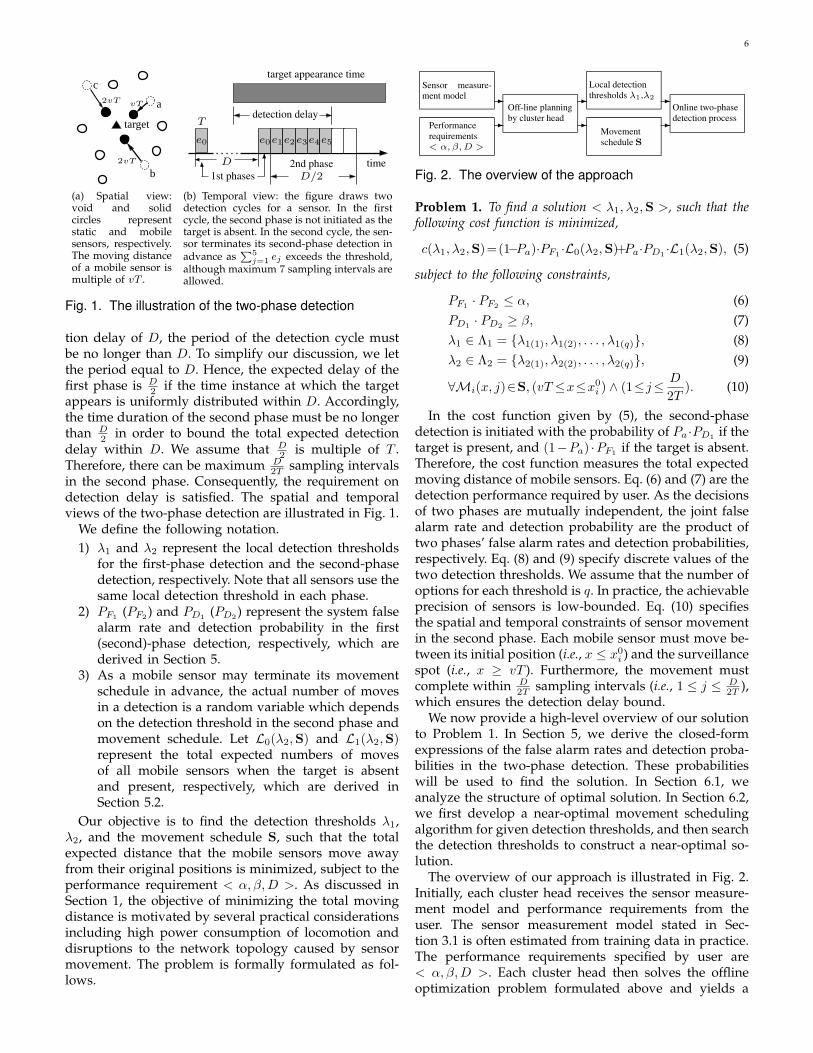
(a) Spatial view:void and solidcircles representstatic and mobilesensors, respectively.The moving distanceof a mobile sensor ismultiple of vT .
e0 e0e1e2e3e4e5
time
T
D
1st phases
2nd phase
D/2
target appearance time
detection delay
(b) Temporal view: the figure draws twodetection cycles for a sensor. In the firstcycle, the second phase is not initiated as thetarget is absent. In the second cycle, the sen-sor terminates its second-phase detection inadvance as
P5j=1 ej exceeds the threshold,
although maximum 7 sampling intervals areallowed.
Fig. 1. The illustration of the two-phase detection
tion delay of D, the period of the detection cycle mustbe no longer than D. To simplify our discussion, we letthe period equal to D. Hence, the expected delay of thefirst phase is D
2 if the time instance at which the targetappears is uniformly distributed within D. Accordingly,the time duration of the second phase must be no longerthan D
2 in order to bound the total expected detectiondelay within D. We assume that D
2 is multiple of T .Therefore, there can be maximum D
2T sampling intervalsin the second phase. Consequently, the requirement ondetection delay is satisfied. The spatial and temporalviews of the two-phase detection are illustrated in Fig. 1.
We define the following notation.1) λ1 and λ2 represent the local detection thresholds
for the first-phase detection and the second-phasedetection, respectively. Note that all sensors use thesame local detection threshold in each phase.
2) PF1 (PF2 ) and PD1 (PD2 ) represent the system falsealarm rate and detection probability in the first(second)-phase detection, respectively, which arederived in Section 5.
3) As a mobile sensor may terminate its movementschedule in advance, the actual number of movesin a detection is a random variable which dependson the detection threshold in the second phase andmovement schedule. Let L0(λ2,S) and L1(λ2,S)represent the total expected numbers of movesof all mobile sensors when the target is absentand present, respectively, which are derived inSection 5.2.
Our objective is to find the detection thresholds λ1,λ2, and the movement schedule S, such that the totalexpected distance that the mobile sensors move awayfrom their original positions is minimized, subject to theperformance requirement < α, β,D >. As discussed inSection 1, the objective of minimizing the total movingdistance is motivated by several practical considerationsincluding high power consumption of locomotion anddisruptions to the network topology caused by sensormovement. The problem is formally formulated as fol-lows.
Sensor measure-
ment model
Performance
requirements
< α, β, D >
Off-line planning
by cluster head
Local detection
thresholds λ1 ,λ2
Movement
schedule S
Online two-phase
detection process
-
-
-
-
-
-
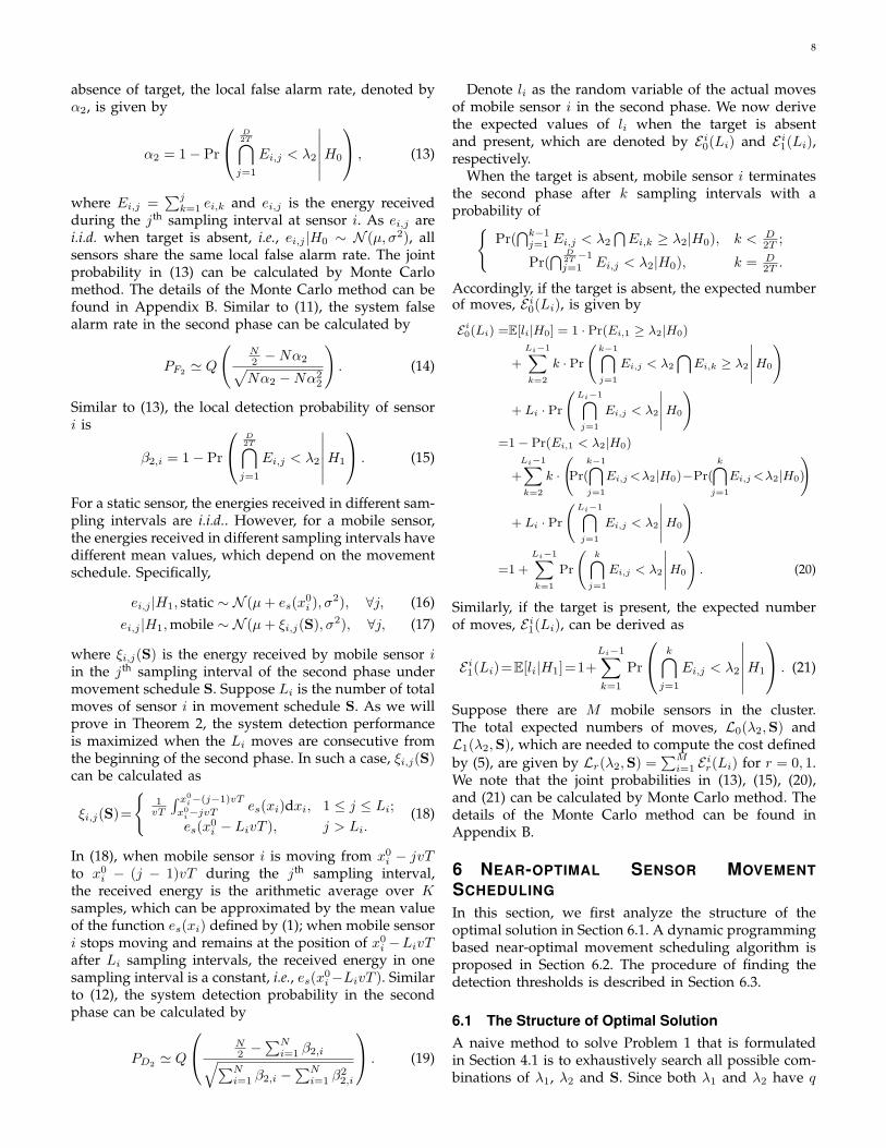
Fig. 2. The overview of the approach
Problem 1. To find a solution < λ1, λ2,S >, such that thefollowing cost function is minimized,
c(λ1, λ2,S)=(1−Pa)·PF1 ·L0(λ2,S)+Pa·PD1 ·L1(λ2,S), (5)
subject to the following constraints,
PF1 · PF2 ≤ α, (6)PD1 · PD2 ≥ β, (7)λ1 ∈ Λ1 = {λ1(1), λ1(2), . . . , λ1(q)}, (8)λ2 ∈ Λ2 = {λ2(1), λ2(2), . . . , λ2(q)}, (9)
∀Mi(x, j)∈S, (vT ≤x≤x0i ) ∧ (1≤j≤ D
2T). (10)
In the cost function given by (5), the second-phasedetection is initiated with the probability of Pa ·PD1 if thetarget is present, and (1−Pa) ·PF1 if the target is absent.Therefore, the cost function measures the total expectedmoving distance of mobile sensors. Eq. (6) and (7) are thedetection performance required by user. As the decisionsof two phases are mutually independent, the joint falsealarm rate and detection probability are the product oftwo phases’ false alarm rates and detection probabilities,respectively. Eq. (8) and (9) specify discrete values of thetwo detection thresholds. We assume that the number ofoptions for each threshold is q. In practice, the achievableprecision of sensors is low-bounded. Eq. (10) specifiesthe spatial and temporal constraints of sensor movementin the second phase. Each mobile sensor must move be-tween its initial position (i.e., x ≤ x0
i ) and the surveillancespot (i.e., x ≥ vT ). Furthermore, the movement mustcomplete within D
2T sampling intervals (i.e., 1 ≤ j ≤ D2T ),
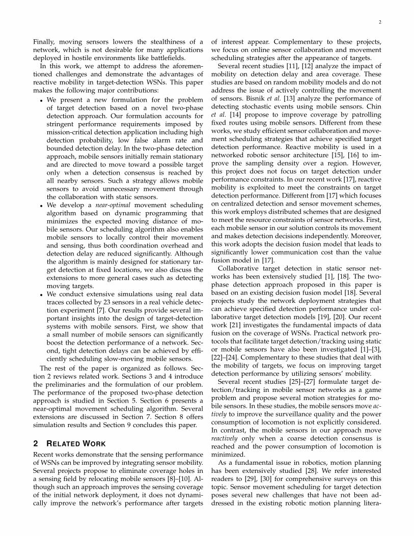
which ensures the detection delay bound.We now provide a high-level overview of our solution
to Problem 1. In Section 5, we derive the closed-formexpressions of the false alarm rates and detection proba-bilities in the two-phase detection. These probabilitieswill be used to find the solution. In Section 6.1, weanalyze the structure of optimal solution. In Section 6.2,we first develop a near-optimal movement schedulingalgorithm for given detection thresholds, and then searchthe detection thresholds to construct a near-optimal so-lution.
The overview of our approach is illustrated in Fig. 2.Initially, each cluster head receives the sensor measure-ment model and performance requirements from theuser. The sensor measurement model stated in Sec-tion 3.1 is often estimated from training data in practice.The performance requirements specified by user are< α, β, D >. Each cluster head then solves the offlineoptimization problem formulated above and yields a

7
solution < λ1, λ2,S >. Finally, each cluster head sendsthe local detection thresholds and movement schedule toeach sensor, which starts the online two-phase detection.
4.2 A Numerical Example
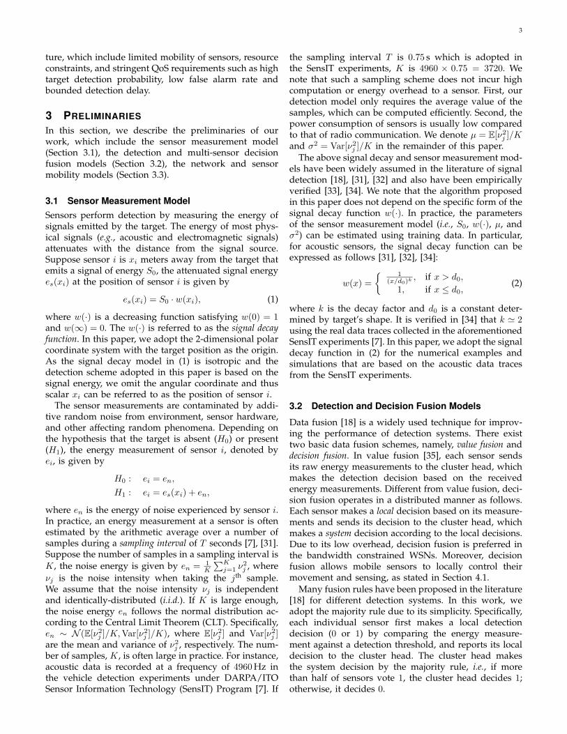
We now illustrate our problem and the basic approachusing a numerical example. To simplify the discussion,we assume that there is only one surveillance spot.We also assume that, after a possible target appears, adecision consensus is always reached in the first phaseof detection, which triggers all mobile sensors to movetoward the surveillance spot. The required false alarmrate and detection probability (i.e., α and β) are 5% and75%, respectively. The minimum movement speed ofmobile sensors is 1 m/s. During initialization, the clusterhead estimates the parameters of sensor measurementmodel using a real data set obtained from [7] (the detailsof experimental settings are given in Section 8).
We now discuss three different cases: a) if all sen-sors are static, 14 sensors will be needed to achievethe required detection performance within a delay of2 seconds as shown in Fig. 3(a); b) If the allowabledetection delay is 7 seconds, 10 mobile sensors will beneeded as they can move closer to the target resultingin higher SNRs; c) If a detection delay of 15 seconds isallowed, only 7 mobile sensors are needed as illustratedin Fig. 3(c). This is because these sensors are able tomove longer distances toward the surveillance spot thanin case b).
Two important observations can be made from thisexample. First, the detection performance can be signif-icantly improved by taking the advantage of mobilityof sensors. Second, scheduling more mobile sensors tomove toward a possible target results in a shorter de-lay. This observation is particularly important as mostmobile sensor platforms have low movement speeds.
5 PERFORMANCE MODELING OF TWO-PHASEDETECTION
We now derive the false alarm rates and the detectionprobabilities in the two phases of detection which areused in Section 6 to find the solution of our problem.
5.1 First-phase Detection
Since the local false alarm rate does not depend onsensor’s position, according to (3), all sensors have thesame local false alarm rate, denoted by α1, which iscalculated by α1 = Q
(λ1−µ
σ
). Hence, in the absence of
target, the number of positive local decisions follows theBinomial distribution, i.e., Y |H0 ∼ Bin(N, α1). Accordingto the de Moivre-Laplace Theorem [32], the Binomial dis-tribution Bin(N,α1) can be approximated by the normaldistribution N (Nα1, Nα1 − Nα2
1) if N ≥ 10 [38]. Thiscondition can be met in many moderate- to large-scale
Ntarget
gg
g
gg
gg
g
g
gg
g
g
g
50m
?
6
50m� -
(a) 14 static sensors;PF = 5%, PD = 75%,delay is 2 s
Ntarget
w���wAAK
wCCCO
w���� wC
CCO
w
6
w�����
wXXy
wCCCO
w�����
50m
?
6
50m� -
(b) 10 mobile sensors;PF = 5%, PD = 75%,delay is 7 s
Ntarget
w���wAAK
wCCCO
w���� wC
CCO
w
6
w
wXXy
ww
50m
?
6
50m� -
(c) 7 mobile sensors;PF = 5%, PD = 75%,delay is 15 s
Fig. 3. A numerical example of target detection usingstatic or mobile sensors.
network deployments. Therefore, the system false alarmrate in the first phase can be approximated by
PF1 = Pr(
Y ≥ N
2
∣∣∣∣H0
)' Q
(N2 − Nα1√Nα1 − Nα2
1
). (11)
We now derive the system detection probability in thefirst-phase detection. In the presence of target, the localdecision at sensor i, Ii|H1, follows the Bernoulli distri-bution with β1,i as the probability of success, where β1,i
is the local detection probability of sensor i at its originalposition x0
i in the first phase. According to (4), β1,i is cal-culated by β1,i = Q
(λ1−µ−es(x0
i )σ
). As I1|H1, . . . , IN |H1
are mutually independent, the mean and variance ofY |H1 are given by E[Y |H1] =
∑Ni=1 E[Ii|H1] =
∑Ni=1 β1,i
and Var[Y |H1] =∑N
i=1 Var[Ii|H1] =∑N
i=1 β1,i−∑N
i=1 β21,i,
respectively. However, I1|H1, . . . , IN |H1 are not identi-cally distributed, as β1,i depends on sensor’s originalposition. The following lemma proves the condition forthe Lyapunov’s CLT [39]. The proof is in Appendix A1.
Lemma 1. Let {Ii : i = 1, . . . , N} be a sequence of mu-tually independent Bernoulli random variables, the Lyapunovcondition holds for this sequence.
According to Lemma 1 and the Lyapunov’s CLT, Y |H1
follows the normal distribution when N is large, i.e.,Y |H1 ∼ N (
∑Ni=1 β1,i,
∑Ni=1 β1,i −
∑Ni=1 β2
1,i). Hence, thesystem detection probability in the first phase can becalculated by
PD1 ' Q
N2 −
∑Ni=1 β1,i√∑N
i=1 β1,i −∑N
i=1 β21,i
. (12)
5.2 Second-phase Detection
In this section, we analyze the performance of the se-quential detection process in the second phase, whichincludes the false alarm rate, the detection probability,and the expected number of moves under a given move-ment schedule.
We assume that all sensors in the second-phase de-tection have the same detection threshold of λ2. In the
1. All appendices can be found in the supplemental materials of thispaper, which are available in the IEEE Digital Library.
8
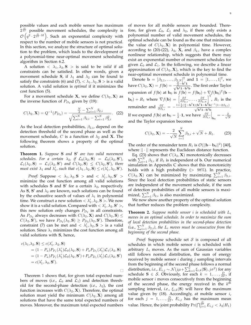
absence of target, the local false alarm rate, denoted byα2, is given by
α2 = 1 − Pr
D2T∩
j=1
Ei,j < λ2
∣∣∣∣∣∣H0
, (13)
where Ei,j =∑j
k=1 ei,k and ei,j is the energy receivedduring the jth sampling interval at sensor i. As ei,j arei.i.d. when target is absent, i.e., ei,j |H0 ∼ N (µ, σ2), allsensors share the same local false alarm rate. The jointprobability in (13) can be calculated by Monte Carlomethod. The details of the Monte Carlo method can befound in Appendix B. Similar to (11), the system falsealarm rate in the second phase can be calculated by
PF2 ' Q
(N2 − Nα2√Nα2 − Nα2
2
). (14)
Similar to (13), the local detection probability of sensori is
β2,i = 1 − Pr
D2T∩
j=1
Ei,j < λ2
∣∣∣∣∣∣H1
. (15)
For a static sensor, the energies received in different sam-pling intervals are i.i.d.. However, for a mobile sensor,the energies received in different sampling intervals havedifferent mean values, which depend on the movementschedule. Specifically,
ei,j |H1, static ∼ N (µ + es(x0i ), σ
2), ∀j, (16)ei,j |H1, mobile ∼ N (µ + ξi,j(S), σ2), ∀j, (17)
where ξi,j(S) is the energy received by mobile sensor iin the jth sampling interval of the second phase undermovement schedule S. Suppose Li is the number of totalmoves of sensor i in movement schedule S. As we willprove in Theorem 2, the system detection performanceis maximized when the Li moves are consecutive fromthe beginning of the second phase. In such a case, ξi,j(S)can be calculated as
ξi,j(S)=
{1
vT
∫ x0i−(j−1)vT
x0i−jvT
es(xi)dxi, 1 ≤ j ≤ Li;es(x0
i − LivT ), j > Li.(18)
In (18), when mobile sensor i is moving from x0i − jvT
to x0i − (j − 1)vT during the jth sampling interval,
the received energy is the arithmetic average over Ksamples, which can be approximated by the mean valueof the function es(xi) defined by (1); when mobile sensori stops moving and remains at the position of x0
i −LivTafter Li sampling intervals, the received energy in onesampling interval is a constant, i.e., es(x0
i −LivT ). Similarto (12), the system detection probability in the secondphase can be calculated by
PD2 ' Q
N2 −
∑Ni=1 β2,i√∑N
i=1 β2,i −∑N
i=1 β22,i
. (19)
Denote li as the random variable of the actual movesof mobile sensor i in the second phase. We now derivethe expected values of li when the target is absentand present, which are denoted by E i
0(Li) and E i1(Li),
respectively.When the target is absent, mobile sensor i terminates
the second phase after k sampling intervals with aprobability of{
Pr(∩k−1
j=1 Ei,j < λ2
∩Ei,k ≥ λ2|H0), k < D
2T ;
Pr(∩ D
2T −1j=1 Ei,j < λ2|H0), k = D
2T .
Accordingly, if the target is absent, the expected numberof moves, E i
0(Li), is given by
Ei0(Li) =E[li|H0] = 1 · Pr(Ei,1 ≥ λ2|H0)
+
Li−1X
k=2
k · Pr
k−1\
j=1
Ei,j < λ2
\
Ei,k ≥ λ2
˛
˛
˛
˛
˛
H0
!
+ Li · Pr
Li−1\
j=1
Ei,j < λ2
˛
˛
˛
˛
˛
H0
!
=1 − Pr(Ei,1 < λ2|H0)
+
Li−1X
k=2
k ·
Pr(
k−1\
j=1
Ei,j <λ2|H0)−Pr(k\
j=1
Ei,j <λ2|H0)
!
+ Li · Pr
Li−1\
j=1
Ei,j < λ2
˛
˛
˛
˛
˛
H0
!
=1 +
Li−1X
k=1
Pr
k\
j=1
Ei,j < λ2
˛
˛
˛
˛
˛
H0
!
. (20)
Similarly, if the target is present, the expected numberof moves, E i
1(Li), can be derived as
E i1(Li)=E[li|H1]=1+
Li−1∑k=1
Pr
k∩j=1
Ei,j < λ2
∣∣∣∣∣∣H1
. (21)
Suppose there are M mobile sensors in the cluster.The total expected numbers of moves, L0(λ2,S) andL1(λ2,S), which are needed to compute the cost definedby (5), are given by Lr(λ2,S) =
∑Mi=1 E i
r(Li) for r = 0, 1.We note that the joint probabilities in (13), (15), (20),and (21) can be calculated by Monte Carlo method. Thedetails of the Monte Carlo method can be found inAppendix B.
6 NEAR-OPTIMAL SENSOR MOVEMENTSCHEDULING
In this section, we first analyze the structure of theoptimal solution in Section 6.1. A dynamic programmingbased near-optimal movement scheduling algorithm isproposed in Section 6.2. The procedure of finding thedetection thresholds is described in Section 6.3.
6.1 The Structure of Optimal SolutionA naive method to solve Problem 1 that is formulatedin Section 4.1 is to exhaustively search all possible com-binations of λ1, λ2 and S. Since both λ1 and λ2 have q
9
possible values and each mobile sensor has maximum2
D2T possible movement schedules, the complexity is
O(q2 · 2 D
2T ·M)
. Such an exponential complexity withrespect to the number of mobile sensors is not practical.In this section, we analyze the structure of optimal solu-tion to the problem, which leads to the development ofa polynomial-time near-optimal movement schedulingalgorithm in Section 6.2.
A solution < λ1, λ2,S > is said to be valid if allconstraints can be satisfied. In other words, given amovement schedule S, if λ1 and λ2 can be found tosatisfy the constraints (6) and (7), < λ1, λ2,S > is a validsolution. A valid solution is optimal if it minimizes thecost function (5).
For a movement schedule X, we define C(λ2,X) asthe inverse function of PD2 given by (19):
C(λ2,X) = Q−1(PD2) =N2 −
∑Ni=1 β2,i√∑N
i=1 β2,i −∑N
i=1 β22,i
. (22)
As the local detection probabilities, β2,i, depend on thedetection threshold of the second phase as well as themovement schedule, C is a function of λ2 and X. Thefollowing theorem shows a property of the optimalsolution.
Theorem 1. Suppose S and S′ are two valid movementschedules. For a certain λ2, if L0(λ2,S) = L0(λ2,S′),L1(λ2,S) = L1(λ2,S′) and C(λ2,S) ≤ C(λ2,S′), theremust exist λ1 and λ′
1, such that c(λ1, λ2,S) ≤ c(λ′1, λ2,S′).
Proof: Suppose < λ1, λ2,S > and < λ′1, λ2,S′ >
minimize the cost function among all valid solutionswith schedules S and S′ for a certain λ2, respectively.As S, S′ and λ2 are known, such solutions can be foundby the exhaustive search of values of λ1 in polynomialtime. We construct a new solution < λ′
1, λ2,S >. We nowshow it is a valid solution. Compared with < λ′
1, λ2,S′ >,this new solution only changes PD2 in all constraints.As PD2 always decreases with C(λ2,X) and C(λ2,S) ≤C(λ2,S′), we have PD2(λ2,S) ≥ PD2(λ2,S′). Therefore,constraint (7) can be met and < λ′
1, λ2,S > is a validsolution. Since λ1 minimizes the cost function among allvalid solutions with S, hence,
c(λ1,λ2,S) ≤ c(λ′1, λ2,S)
= (1 − Pa)PF1(λ′1)L0(λ2,S) + PaPD1(λ
′1)L1(λ2,S)
= (1 − Pa)PF1(λ′1)L0(λ2,S′)+PaPD1(λ
′1)L1(λ2,S′)
= c(λ′1, λ2,S′).
Theorem 1 shows that, for given total expected num-bers of moves (i.e., L0 and L1) and detection thresh-old for the second-phase detection (i.e., λ2), the costfunction increases with C(λ2,X). Therefore, the optimalsolution must yield the minimum C(λ2,X) among allsolutions that have the same total expected numbers ofmoves. Moreover, the maximum total expected numbers
of moves for all mobile sensors are bounded. There-fore, for given L0, L1 and λ2, if there only exists apolynomial number of valid movement schedules, theoptimal schedule can be found as the one that minimizesthe value of C(λ2,X) in polynomial time. However,according to (20)-(22), λ2, X, and β2,i have a complexnonlinear relationship, which suggests that there mayexist an exponential number of movement schedules forgiven L0 and L1. In the following, we describe a linearapproximation of C(λ2,X), which is the key to find thenear-optimal movement schedule in polynomial time.
Denote b = [β2,1, . . . , β2,N ]T and 1 = [1, . . . , 1]T, wehave C(λ2,X) = f(b) =
N2 −bT1√bT1−bTb
. The first order Taylor
expansion of f(b) at b0 is f(b) = f(b0) + ∇f(b0)T(b −b0) + R1 where ∇f(b) =
[∂f
∂β2,1, . . . , ∂f
∂β2,N
]T, R1 is the
remainder and ∂f∂β2,i
= −1+ 12 ( n
2 −bT1)(bT1−bTb)−1(1−2β2,i)√bT1−bTb
.
If we expand f(b) at b0 = 12 ·1, we have ∂f
∂β2,i
∣∣∣b0
= − 2√N
and the Taylor expansion becomes
C(λ2,X) = − 2√N
N∑i=1
β2,i +√
N + R1. (23)
The order of the remainder term R1 is O(||b−b0||2) [40],where || · || represents the Euclidean distance function.
Eq. (23) shows that C(λ2,X) monotonically decreaseswith
∑Ni=1 β2,i if R1 is independent of b. Our numerical
simulation in Appendix C shows that this monotonicityholds with a high probability (> 98%). In practice,C(λ2,X) can be minimized by maximizing
∑Ni=1 β2,i.
Since the local detection probabilities of static sensorsare independent of the movement schedule, if the sumof detection probabilities of all mobile sensors is maxi-mized,
∑Ni=1 β2,i is also maximized.
We now show another property of the optimal solutionthat further reduces the problem complexity.
Theorem 2. Suppose mobile sensor i is scheduled with Li
moves in an optimal schedule. In order to maximize the sumof local detection probabilities in the second-phase detection(i.e.,
∑Ni=1 β2,i), the Li moves must be consecutive from the
beginning of the second phase.
Proof: Suppose schedule set S is composed of allschedules in which mobile sensor i is scheduled witharbitrary Li moves. As the sum of Gaussian variablesstill follows normal distribution, the sum of energyreceived by mobile sensor i during j sampling intervalsfrom the beginning of the second phase follows a normaldistribution, i.e., Ei,j ∼ N (jµ+
∑jk=1 ξi,k(S), jσ2) for any
schedule S ∈ S. Obviously, for each k = 1, . . . , D2T , if
mobile sensor i moves consecutively from the beginningof the second phase, the energy received in the kth
sampling interval, i.e., ξi,k(S) will have the maximumvalue given by (18). Accordingly, at mobile sensor i,for each j = 1, . . . , D
2T , Ei,j has the maximum mean
value. Hence, the joint probability Pr(∩ D
2Tj=1 Ei,j < λ2|H1)
10
is minimized. Therefore, the local detection probabilityof mobile sensor i, β2,i, which is given by (15), ismaximized. If all mobile sensors move in parallel andconsecutively from the beginning of the second-phasedetection, the sum of local detection probabilities in thesecond-phase detection,
∑Ni=1 β2,i, is maximized.
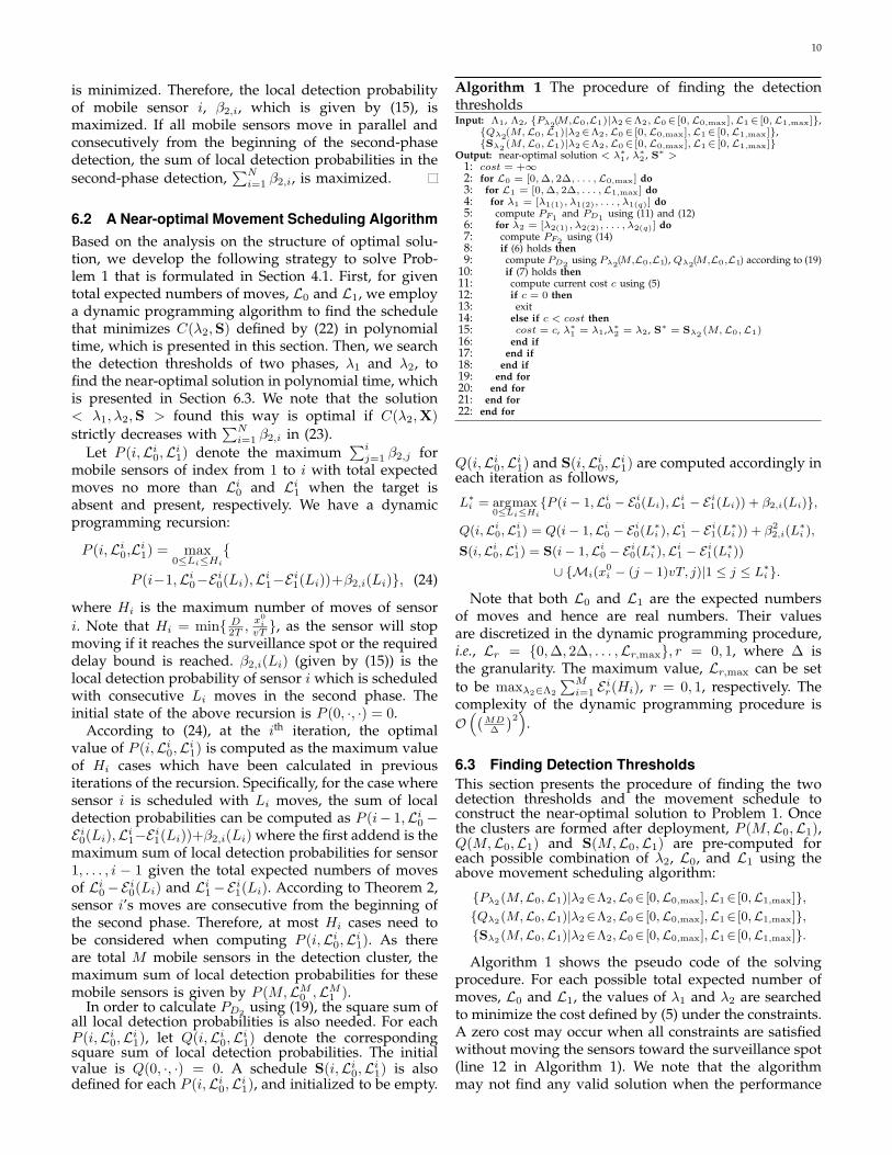
6.2 A Near-optimal Movement Scheduling AlgorithmBased on the analysis on the structure of optimal solu-tion, we develop the following strategy to solve Prob-lem 1 that is formulated in Section 4.1. First, for giventotal expected numbers of moves, L0 and L1, we employa dynamic programming algorithm to find the schedulethat minimizes C(λ2,S) defined by (22) in polynomialtime, which is presented in this section. Then, we searchthe detection thresholds of two phases, λ1 and λ2, tofind the near-optimal solution in polynomial time, whichis presented in Section 6.3. We note that the solution< λ1, λ2,S > found this way is optimal if C(λ2,X)strictly decreases with
∑Ni=1 β2,i in (23).
Let P (i,Li0,Li
1) denote the maximum∑i
j=1 β2,j formobile sensors of index from 1 to i with total expectedmoves no more than Li
0 and Li1 when the target is
absent and present, respectively. We have a dynamicprogramming recursion:
P (i,Li0,Li
1) = max0≤Li≤Hi
{
P (i−1,Li0−E i
0(Li),Li1−E i
1(Li))+β2,i(Li)}, (24)
where Hi is the maximum number of moves of sensori. Note that Hi = min{ D
2T ,x0
i
vT }, as the sensor will stopmoving if it reaches the surveillance spot or the requireddelay bound is reached. β2,i(Li) (given by (15)) is thelocal detection probability of sensor i which is scheduledwith consecutive Li moves in the second phase. Theinitial state of the above recursion is P (0, ·, ·) = 0.
According to (24), at the ith iteration, the optimalvalue of P (i,Li
0,Li1) is computed as the maximum value
of Hi cases which have been calculated in previousiterations of the recursion. Specifically, for the case wheresensor i is scheduled with Li moves, the sum of localdetection probabilities can be computed as P (i− 1,Li
0 −E i0(Li),Li
1−E i1(Li))+β2,i(Li) where the first addend is the
maximum sum of local detection probabilities for sensor1, . . . , i − 1 given the total expected numbers of movesof Li
0 −E i0(Li) and Li
1 −E i1(Li). According to Theorem 2,
sensor i’s moves are consecutive from the beginning ofthe second phase. Therefore, at most Hi cases need tobe considered when computing P (i,Li
0,Li1). As there
are total M mobile sensors in the detection cluster, themaximum sum of local detection probabilities for thesemobile sensors is given by P (M,LM
0 ,LM1 ).
In order to calculate PD2 using (19), the square sum ofall local detection probabilities is also needed. For eachP (i,Li
0,Li1), let Q(i,Li
0,Li1) denote the corresponding
square sum of local detection probabilities. The initialvalue is Q(0, ·, ·) = 0. A schedule S(i,Li
0,Li1) is also
defined for each P (i,Li0,Li
1), and initialized to be empty.
Algorithm 1 The procedure of finding the detectionthresholdsInput: Λ1, Λ2, {Pλ2(M,L0,L1)|λ2∈Λ2,L0∈ [0,L0,max],L1∈ [0,L1,max]},
{Qλ2(M,L0,L1)|λ2∈Λ2,L0∈ [0,L0,max],L1∈ [0,L1,max]},{Sλ2 (M,L0,L1)|λ2∈Λ2,L0∈ [0,L0,max],L1∈ [0,L1,max]}
Output: near-optimal solution < λ∗1 , λ∗
2 , S∗ >1: cost = +∞2: for L0 = [0, ∆, 2∆, . . . ,L0,max] do3: for L1 = [0, ∆, 2∆, . . . ,L1,max] do4: for λ1 = [λ1(1), λ1(2), . . . , λ1(q)] do5: compute PF1 and PD1 using (11) and (12)6: for λ2 = [λ2(1), λ2(2), . . . , λ2(q)] do7: compute PF2 using (14)8: if (6) holds then9: compute PD2 using Pλ2(M,L0,L1), Qλ2(M,L0,L1) according to (19)
10: if (7) holds then11: compute current cost c using (5)12: if c = 0 then13: exit14: else if c < cost then15: cost = c, λ∗
1 = λ1,λ∗2 = λ2, S∗ = Sλ2 (M,L0,L1)
16: end if17: end if18: end if19: end for20: end for21: end for22: end for
Q(i,Li0,Li
1) and S(i,Li0,Li
1) are computed accordingly ineach iteration as follows,
L∗i = argmax
0≤Li≤Hi
{P (i − 1,Li0 − E i
0(Li),Li1 − E i
1(Li)) + β2,i(Li)},
Q(i,Li0,Li
1) = Q(i − 1,Li0 − E i
0(L∗i ),Li
1 − E i1(L
∗i )) + β2
2,i(L∗i ),
S(i,Li0,Li
1) = S(i − 1,Li0 − E i
0(L∗i ),Li
1 − E i1(L
∗i ))
∪ {Mi(x0i − (j − 1)vT, j)|1 ≤ j ≤ L∗
i }.
Note that both L0 and L1 are the expected numbersof moves and hence are real numbers. Their valuesare discretized in the dynamic programming procedure,i.e., Lr = {0,∆, 2∆, . . . ,Lr,max}, r = 0, 1, where ∆ isthe granularity. The maximum value, Lr,max can be setto be maxλ2∈Λ2
∑Mi=1 E i
r(Hi), r = 0, 1, respectively. Thecomplexity of the dynamic programming procedure isO“
`
MD∆
´2”
.
6.3 Finding Detection ThresholdsThis section presents the procedure of finding the twodetection thresholds and the movement schedule toconstruct the near-optimal solution to Problem 1. Oncethe clusters are formed after deployment, P (M,L0,L1),Q(M,L0,L1) and S(M,L0,L1) are pre-computed foreach possible combination of λ2, L0, and L1 using theabove movement scheduling algorithm:
{Pλ2(M,L0,L1)|λ2∈Λ2,L0∈ [0,L0,max],L1∈ [0,L1,max]},{Qλ2(M,L0,L1)|λ2∈Λ2,L0∈ [0,L0,max],L1∈ [0,L1,max]},{Sλ2(M,L0,L1)|λ2∈Λ2,L0∈ [0,L0,max],L1∈ [0,L1,max]}.
Algorithm 1 shows the pseudo code of the solvingprocedure. For each possible total expected number ofmoves, L0 and L1, the values of λ1 and λ2 are searchedto minimize the cost defined by (5) under the constraints.A zero cost may occur when all constraints are satisfiedwithout moving the sensors toward the surveillance spot(line 12 in Algorithm 1). We note that the algorithmmay not find any valid solution when the performance
11
requirements exceed the maximum detection capabilityof the cluster. For instance, the constraint on the systemdetection probability may not be satisfied even whenall mobile sensors have been scheduled with the max-imum number of moves under the delay bound. Thecomplexity of Algorithm 1 is O
“
`
MD∆
´2 · q2”
, which isdependent on the granularities ∆ and q. The smaller∆ or greater q yields better solution at the price ofhigher computation and storage overhead. Therefore, inpractice, we can balance the solution quality and theoverhead with respect to the capability of cluster headby choosing proper granularities.
7 EXTENSIONS
We now discuss several open issues that have not beenaddressed in previous sections and investigate theirimpacts on the performance of the proposed algorithm.We also discuss how to extend our approach to addressthem.
7.1 Estimating Target Appearance Probability
We assume that the probability that a target appears atthe surveillance spot is Pa in the problem formulation.From the structure of the problem formulation, Pa onlyaffects the cost function (5). Hence, when the estimatedPa is inaccurate, the solution found can still satisfy theconstraints (6)-(10) at the expense of longer movementdistance of mobile sensors. In other words, inaccurate Pa
still yields valid solution.We now discuss how to estimate Pa when it is not
known a priori. As many monitored physical phenomena(e.g., moving vehicle) are often spatially correlated, oneapproach is to obtain the Pa from a closely located neigh-bour cluster which has accurate Pa. Another approachis to estimate Pa based on detection history. The basicidea is as follows. The initial Pa can be set to be thebest guess. As inaccurate Pa still yields valid solution,i.e., any target can be detected with a probability of βwhile the false alarm rate is α, after n detections, thenumber of positive final decisions (denoted by n+) isn+ ' βp+α(n−p), where p is the true number of targetappearances which is unknown. Note that βp is thenumber of correct detections, and α(n−p) is the numberof false alarms. Therefore, the Pa can be estimated asPa = p
n ' n+−nαn(β−α) . We note that this method can also be
applied to update Pa periodically so that the detectioncluster can adapt to the change of target appearanceprobability.
7.2 Incorporating Different Sensor Mobility Models
In previous sections, we assume the free mobility modelfor mobile sensors, i.e., the mobile sensors are able tomove continuously in any direction. We now discusshow our approach can be applied to other mobilitymodels.
di
Oi
x
target
√
d2
i+ x2
i
x0
i
xi
sensor i
ai
bi
(a) Case 1: ai ≤ 0
di
Oi
x
target
√
d2
i+ x2
i
x0
i
xi
sensor i
ai
bi
(b) Case 2: ai > 0
Fig. 4. Two cases of the straight trail mobility model
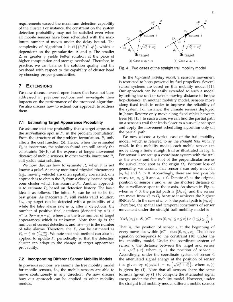
In the hop-based mobility model, a sensor’s movementis restricted to hops powered by fuel-propellers. Severalsensor systems are based on this mobility model [41].Our approach can be easily extended to such a modelby setting the unit of sensor moving distance to be thehop-distance. In another mobility model, sensors movealong fixed trails in order to improve the reliability ofthe system. For instance, the climate sensors deployedin James Reserve only move along fixed cables betweentrees [4], [15]. In such a case, we can find the partial pathon a sensor’s trail that leads closer to a surveillance spotand apply the movement scheduling algorithm only onthe partial path.
We now discuss a typical case of the trail mobilitymodel, which is referred to as the straight trail mobilitymodel. In this mobility model, each mobile sensor canmove along a finite straight trail as illustrated in Fig. 4.For sensor i, we set up a coordinate system with the trailas the x-axis and the foot of the perpendicular acrossthe surveillance spot as the origin Oi. Without loss ofgenerality, we assume that sensor i can only move in[ai, bi] and bi > 0. Accordingly, there are two possiblecases, i.e., ai ≤ 0 and ai > 0. Denote x0
i as the originalposition of sensor i and di as the shortest distance ofthe surveillance spot to the x-axis. As shown in Fig. 4,when ai ≤ 0, the partial path is [Oi, x
0i ] and the sensor
can move from x0i to Oi because it achieves the highest
SNR at Oi. In the case of ai > 0, the partial path is [ai, x0i ].
Therefore, the spatial and temporal constraints of sensormovement under the straight trail mobility model is
∀Mi(x, j)∈S, (vT + max{0, ai}≤x≤x0i ) ∧ (1≤j≤ D
2T).
That is, the position of sensor i at the beginning ofevery move lies within [vT + max{0, ai}, x0
i ]. The aboveequation corresponds to the constraint (10) under thefree mobility model. Under the coordinate system ofsensor i, the distance between the target and sensori is
√d2
i + x2i where xi is the position of sensor i.
Accordingly, under the coordinate system of sensor i,the attenuated signal energy at the position of sensori is given by e′s(xi|di) = es
(√x2
i + d2i
), where es(·)
is given by (1). Note that all sensors share the sameformula (given by (1)) to compute the attenuated signalenergy under the free mobility model. However, underthe straight trail mobility model, different mobile sensors
12
have different formulas defined in their own coordinatesystems. Nevertheless, the structure of the optimal solu-tion does not change. Specifically, by replacing es(xi) in(16) and (18) with e′s(xi|di), the near-optimal movementscheduling algorithm also works under the straight trailmobility model.
7.3 Handling Heterogeneous SensorsIn this section, we discuss the basic idea of extending ourapproach to the networks that are composed of severaltypes of sensors (e.g., acoustic and seismic sensors).Suppose there are total m types of sensors and eachsensing modality has a specific measurement model asstated in Section 3.1. We summarize the major extensionsto our approach as follows.
1) As different sensing modalities should have dif-ferent detection thresholds, the solution of ourproblem becomes < ~λ1, ~λ2,S >, where ~λk =[λk,1, · · · , λk,m]T and λk,j is the detection thresholdfor modality j in the kth phase.
2) In the absence of target, the measurements of dif-ferent modalities are not identically distributed.However, as a number of sensors take part inthe decision fusion, the sum of positive decisionsY |H0 approximately follows the normal distribu-tion according to the Lyapunov’s CLT. As a result,PF1 and PF2 have similar expressions as (12) and(19). Specifically, PF1 and PF2 can be obtained byreplacing β1,i in (12) with α1,i, and β2,i in (19) withα2,i, respectively, where αk,i is the local false alarmrate of sensor i in the kth phase. Hence, the systemfalse alarm rate and detection probability can becomputed with closed-form expressions.
3) Theorem 1 and Theorem 2 still hold after replacingλ1 and λ2 by ~λ1 and ~λ2, respectively, as these twotheorems do not depend on the algebraic represen-tation (scalar or vector) of the detection thresholds.
The complexity of Algorithm 1 will increase toO“
`
MD∆
´2q2m
”
, as iterating each ~λ1 and ~λ2 has a com-plexity of O(q2m). Note that the decisions of heteroge-neous sensors are fused according to the majority rule.More efficient fusion rules that account for the differencein fidelity characteristics of sensors might be incorpo-rated into our approach, e.g., weighted decision fusion.However, we omit the investigation of the optimal fusionrules for heterogeneous sensors due to space limit.
7.4 Detecting Moving TargetsIn previous sections, we assume that the target remainsstationary at the surveillance spot. In many applications,the target is mobile. In this section, we briefly discusshow to extend our approach to address the problem ofdetecting moving targets. Note that the approach pre-sented below can also be extended to the more generalcase where the target is spatially distributed, as long asthe spatial distribution of the target can be estimated.
We face several challenges in detecting moving targets.First, the accurate position of the moving target is oftenunknown in practice. Moreover, the signal attenuationcharacteristic of the moving target varies over time.Therefore, it is difficult to find the optimal solution thatachieves the specified detection performance require-ment. Our basic idea to address this issue is to treat themoving target as a stationary target with conservativesource energy estimate. For a cluster, we consider theperformance of detecting the moving target with sourceenergy of S0 in a region A that is around the surveillancespot. We assume the time that the target is in A islonger than the required detection delay D. Denotedi,max as the maximum distance from sensor i to anypoint in A. Hence, the minimum energy received bysensor i when the target is in A, denoted by si,min, issi,min = S0w(di,max). If a stationary target with sourceenergy of S′
0 is at the surveillance spot, the signal energyreceived by sensor i is s′i = S′
0w(x0i ). If we let S′
0 =mini
{S0w(di,max)
w(x0i )
}, we have si,min ≥ s′i for any sensor i in
the cluster. As a result, the detection performance for themoving target with source energy of S0 will not be worsethan that for the stationary target at the surveillancespot with source energy of S′
0. Therefore, the solutionfound by our algorithm with target source energy ofS′
0 is a valid solution for detecting the moving targetwith source energy of S0. Note that the region A canbe chosen according to the mobility model of the target.For instance, if the target path is known, the region A canbe reduced to the path section around the surveillancespot. The above scheme will achieve better performancewhen it is integrated with a target tracking protocol thatcan determine the trajectory of a moving target.
8 PERFORMANCE EVALUATION
8.1 Simulation Methodology and SettingsWe conduct extensive simulations using the real datatraces collected in the SensIT vehicle detection experi-ments [7]. In the experiment, 75 sensors are deployedto detect military vehicles driving through several in-tersected roads. The data set used in our simulationsincludes the acoustic time series recorded by 23 nodesat the frequency of 4960 Hz and ground truth. Receivedenergy is calculated every 0.75 s. Each run is namedafter the vehicle type and the number of run, e.g., AAV3stands for the third run when an Assault AmphibianVehicle (AAV) drives through the road. We refer to[7] for more detailed setup of the experiment. In oursimulations, the acoustic data of AAV3-AAV11 are used.
As the data are collected by fixed sensors, they cannot be directly used in our simulations. We generatedata for our simulations as follows. For each energymeasurement collected by a sensor, we compute thedistance between the sensor and the vehicle from theground truth data. When a sensor makes a measurementin our simulations, the energy is set to be the realmeasurement gathered at a similar distance to target.
13
75m
?
6
50m
?
6
50m� -
N
N
N
N
cc
c
cc
sCCO
s6
sXXy
sAAK
sCCO
bfixed sensorrmobile sensor
N surveillance spot
��
��
c c
� ���
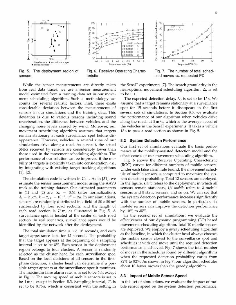
Fig. 5. The deployment region ofsensors
30
40
50
60
70
80
90
100
0.5 1 1.5 2 2.5 3 3.5 4 4.5 5
Det
ectio
npr
obab
ility
(%)
False alarm rate (%)
static1/4 mobile1/2 mobile3/4 mobileall mobile
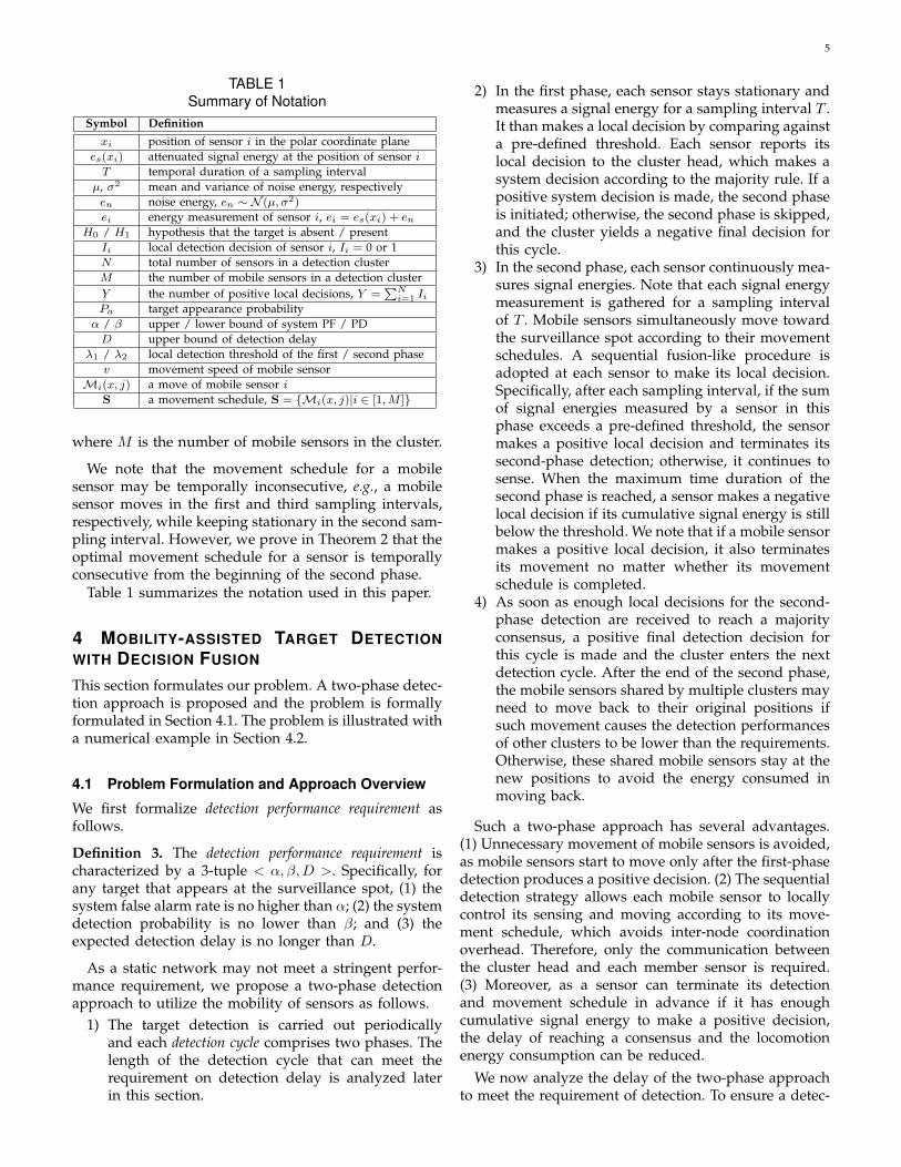
Fig. 6. Receiver Operating Charac-teristic
0
10
20
30
40
50
60
82 84 86 88 90 92The
num
ber
of
tota
lsc
hed
ule
dm
oves
Requested PD (%)
DPgreedy
Fig. 7. The number of total sched-uled moves vs. requested PD
While the sensor measurements are directly takenfrom real data traces, we use a sensor measurementmodel estimated from a training data set in our move-ment scheduling algorithm. Such a methodology ac-counts for several realistic factors. First, there existsconsiderable deviation between the measurements ofsensors in our simulations and the training data. Thisdeviation is due to various reasons including soundreverberation, the difference between vehicles, and thechanging noise levels caused by wind. Moreover, ourmovement scheduling algorithm assumes that targetsremain stationary at each surveillance spot before dis-appearance. However, vehicles in several runs of oursimulations drive along a road. As a result, the actualSNRs received by sensors are considerably lower thanthose used in the movement scheduling algorithm. Theperformance of our solution can be improved if the mo-bility of targets is explicitly taken into consideration, e.g.,by integrating with existing target tracking algorithms[1], [2].
The simulation code is written in C++. As in [31], weestimate the sensor measurement model using the AAV3track as the training dataset. Our estimated parametersin (1) and (2) are: S0 = 0.51 (after normalization),d0 = 2.6 m, k = 2, µ = 10−4, σ2 = 2µ. In our simulations,sensors are randomly distributed in a field of 50×50 m2
surrounded by four road sections, and the length ofeach road section is 75 m, as illustrated in Fig. 5. Asurveillance spot is located at the center of each roadsection. In real scenarios, surveillance spots would beidentified by the network after the deployment.
The total simulation time is 3× 10⁷ seconds, and eachtarget appearance lasts for 15 seconds. The probabilitythat the target appears at the beginning of a samplinginterval is set to be 5%. Each sensor in the deploymentregion belongs to four clusters. A sensor is randomlyselected as the cluster head for each surveillance spot.Based on the local decisions of all sensors in the first-phase detection, a cluster head can determine if a pos-sible target appears at the surveillance spot it monitors.The maximum false alarm rate, α, is set to be 5%, exceptin Fig. 6. The moving speed of mobile sensors is set tobe 1 m/s except in Section 8.3. Sampling interval, T , isset to be 0.75 s, which is consistent with the setting in
the SensIT experiments [7]. The search granularity in thenear-optimal movement scheduling algorithm, ∆, is setto be 0.1.
The expected detection delay, D, is set to be 15 s. Weassume that a target remains stationary at a surveillancespot for 15 seconds before it disappears in the firstseveral sets of simulations. In Section 8.5, we evaluatethe performance of our algorithm when vehicles drivealong the roads at 5 m/s, which is the average speed ofthe vehicles in the SensIT experiments. It takes a vehicle15 s to pass a road section as shown in Fig. 5.
8.2 System Detection PerformanceOur first set of simulations evaluate the basic perfor-mance of the mobility-assisted detection model and theeffectiveness of our movement scheduling algorithm.
Fig. 6 shows the Receiver Operating Characteristic(ROC) curves for different numbers of mobile sensors.Under each false alarm rate bound, the movement sched-ule of mobile sensors is computed to maximize the sys-tem detection probability. Total 12 sensors are deployed.In the figure, static refers to the deployment in which allsensors remain stationary, 1/4 mobile refers to 3 mobilesensors and 9 static sensors, and so on. We can see thatthe system detection performance increases significantlywith the number of mobile sensors. In particular, sixmobile sensors can improve the detection performanceby 10% to 35%.
In the second set of simulations, we evaluate theeffectiveness of our dynamic programming (DP) basedmovement scheduling algorithm. Total 10 mobile sensorsare deployed. We employ a greedy scheduling algorithmas the baseline, in which the cluster head always choosesthe mobile sensor closest to the surveillance spot andschedules it with one move until the required detectionperformance is achieved. Fig. 7 shows the total numberof moves in the schedules found by different algorithmswhen the requested detection probability varies from82% to 92%. As shown in Fig 7, our algorithm schedulesabout 10 fewer moves than the greedy algorithm.
8.3 Impact of Mobile Sensor SpeedIn this set of simulations, we evaluate the impact of mo-bile sensor speed on the system detection performance.
14
82
84
86
88
90
92
94
96
82 84 86 88 90 92 94
Det
ectio
npr
obab
ility
(%)
Requested PD (%)
0.20.40.60.81.0
Fig. 8. Actual PD vs. requested PDwith different sensor speeds
0
10
20
30
40
50
60
70
80
82 84 86 88 90 92 94
The
num
ber
ofto
talm
oves
Requested PD (%)
0.20.40.60.81.0
Fig. 9. The number of total movesvs. requested PD with different sen-sor speeds
70
75
80
85
90
95
100
82 84 86 88 90 92 94
Det
ectio
npr
obab
ility
(%)
Requested PD (%)
5.14dB5.72dB6.23dB7.22dB8.15dB
Fig. 10. Actual PD vs. requestedPD with different SNRs
0
10
20
30
40
50
60
70
82 84 86 88 90 92 94
The
num
ber
ofto
talm
oves
Requested PD (%)
5.14dB5.72dB6.23dB7.22dB8.15dB
Fig. 11. The number of total movesvs. requested PD with differentSNRs
55
60
65
70
75
80
85
90
95
4 6 8 10 12 14 16 18
Det
ectio
npr
obab
ility
(%)
The number of sensors
static1/2 mobileall mobile
Fig. 12. PD vs. the number of sen-sors when detecting moving targets
70
72
74
76
78
80
4 6 8 10 12 14 16 18
Aver
age
det
ecti
on
del
ay(%
)
The number of sensors
static1/2 mobileall mobile
Fig. 13. Detection delay vs. thenumber of sensors
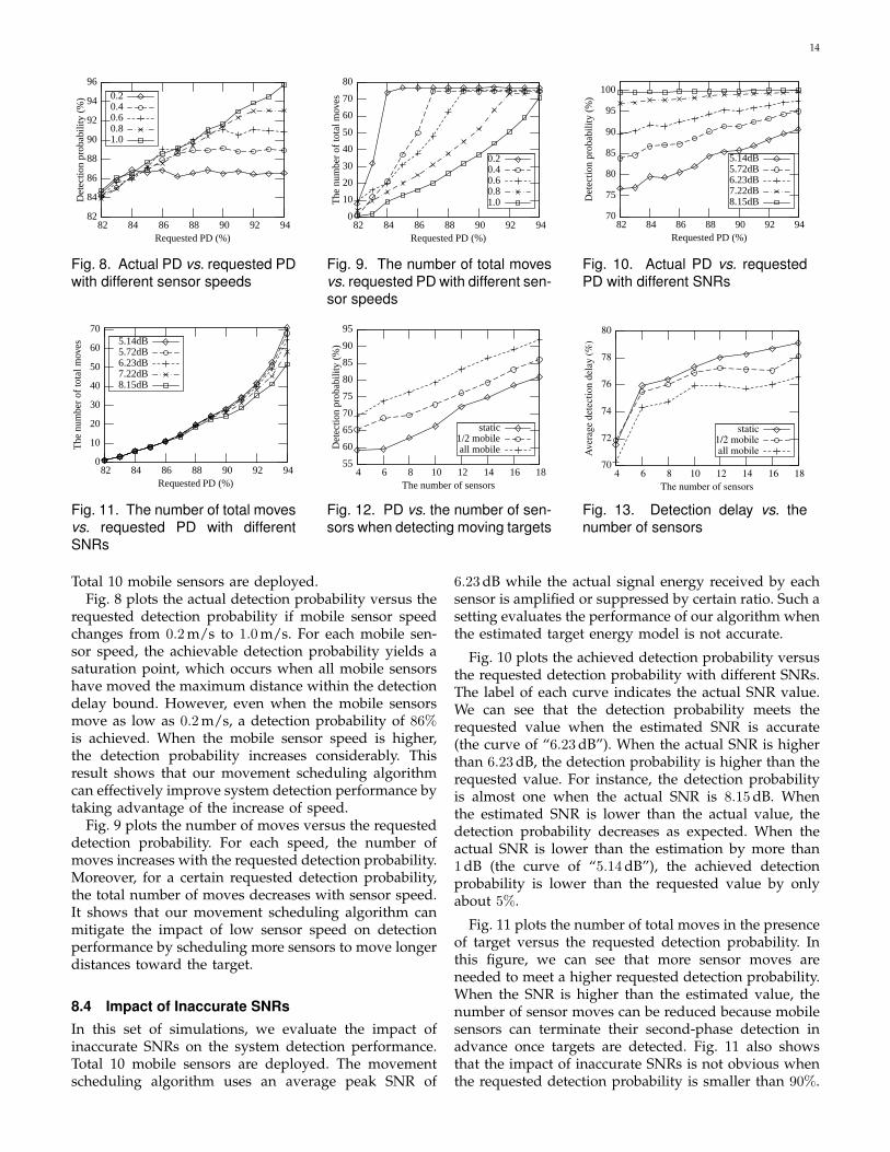
Total 10 mobile sensors are deployed.Fig. 8 plots the actual detection probability versus the
requested detection probability if mobile sensor speedchanges from 0.2 m/s to 1.0 m/s. For each mobile sen-sor speed, the achievable detection probability yields asaturation point, which occurs when all mobile sensorshave moved the maximum distance within the detectiondelay bound. However, even when the mobile sensorsmove as low as 0.2 m/s, a detection probability of 86%is achieved. When the mobile sensor speed is higher,the detection probability increases considerably. Thisresult shows that our movement scheduling algorithmcan effectively improve system detection performance bytaking advantage of the increase of speed.
Fig. 9 plots the number of moves versus the requesteddetection probability. For each speed, the number ofmoves increases with the requested detection probability.Moreover, for a certain requested detection probability,the total number of moves decreases with sensor speed.It shows that our movement scheduling algorithm canmitigate the impact of low sensor speed on detectionperformance by scheduling more sensors to move longerdistances toward the target.
8.4 Impact of Inaccurate SNRsIn this set of simulations, we evaluate the impact ofinaccurate SNRs on the system detection performance.Total 10 mobile sensors are deployed. The movementscheduling algorithm uses an average peak SNR of
6.23 dB while the actual signal energy received by eachsensor is amplified or suppressed by certain ratio. Such asetting evaluates the performance of our algorithm whenthe estimated target energy model is not accurate.
Fig. 10 plots the achieved detection probability versusthe requested detection probability with different SNRs.The label of each curve indicates the actual SNR value.We can see that the detection probability meets therequested value when the estimated SNR is accurate(the curve of “6.23 dB”). When the actual SNR is higherthan 6.23 dB, the detection probability is higher than therequested value. For instance, the detection probabilityis almost one when the actual SNR is 8.15 dB. Whenthe estimated SNR is lower than the actual value, thedetection probability decreases as expected. When theactual SNR is lower than the estimation by more than1 dB (the curve of “5.14 dB”), the achieved detectionprobability is lower than the requested value by onlyabout 5%.
Fig. 11 plots the number of total moves in the presenceof target versus the requested detection probability. Inthis figure, we can see that more sensor moves areneeded to meet a higher requested detection probability.When the SNR is higher than the estimated value, thenumber of sensor moves can be reduced because mobilesensors can terminate their second-phase detection inadvance once targets are detected. Fig. 11 also showsthat the impact of inaccurate SNRs is not obvious whenthe requested detection probability is smaller than 90%.
15
0
20
40
60
80
100
9841071156318.112.612.011.211.29.69.39.07.5
Det
ectio
npr
obab
ility
(%)
AAV run and SNR (dB)
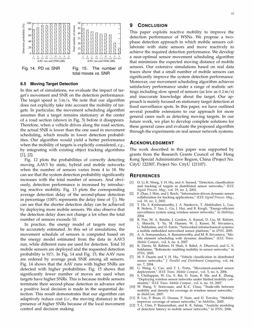
Fig. 14. PD vs. SNR
20
25
30
35
40
45
50
9841071156318.112.612.011.211.29.69.39.07.5
Tota
lnum
ber
ofm
oves
AAV run and SNR (dB)
Fig. 15. The number oftotal moves vs. SNR
8.5 Moving Target DetectionIn this set of simulations, we evaluate the impact of tar-get’s movement and SNR on the detection performance.The target speed is 5 m/s. We note that our algorithmdoes not explicitly take into account the mobility of tar-gets. In particular, the movement scheduling algorithmassumes that a target remains stationary at the centerof a road section (shown in Fig. 5) before it disappears.Therefore, when a vehicle drives along the road section,the actual SNR is lower than the one used in movementscheduling, which results in lower detection probabil-ities. Our algorithm would yield a better performancewhen the mobility of targets is explicitly considered, e.g.,by integrating with existing object tracking algorithms[1], [2].
Fig. 12 plots the probabilities of correctly detectingmoving AAV3 by static, hybrid and mobile networkswhen the number of sensors varies from 4 to 18. Wecan see that the system detection probability significantlyincreases with the total number of sensors. And obvi-ously, detection performance is increased by introduc-ing reactive mobility. Fig. 13 plots the correspondingaverage detection delay of the second-phase detectionin percentage (100% represents the delay time of D
2 ). Wecan see that the shorter detection delay can be achievedby deploying more mobile sensors. We also observe thatthe detection delay does not change a lot when the totalnumber of sensors exceeds 10.
In practice, the energy model of targets may notbe accurately estimated. In this set of simulations, themovement schedule of sensors is computed based onthe energy model estimated from the data in AAV3run, while different runs are used for detection. Total 10mobile sensors are deployed and the requested detectionprobability is 92%. In Fig. 14 and Fig. 15, the AAV runsare ordered by average peak SNR among all sensors.Fig. 14 shows that the AAV runs with higher SNRs aredetected with higher probabilities. Fig. 15 shows thatsignificantly fewer number of moves are used whentargets have higher SNRs. This is because mobile sensorsterminate their second-phase detection in advance aftera positive local decision is made in the sequential de-tection. This result demonstrates that our algorithm canadaptively reduce cost (i.e., the moving distance) in thepresence of higher SNRs because of the local movementcontrol and decision making.
9 CONCLUSION
This paper exploits reactive mobility to improve thedetection performance of WSNs. We propose a two-phase detection approach in which mobile sensors col-laborate with static sensors and move reactively toachieve the required detection performance. We developa near-optimal sensor movement scheduling algorithmthat minimizes the expected moving distance of mobilesensors. Our extensive simulations based on real datatraces show that a small number of mobile sensors cansignificantly improve the system detection performance.Moreover, our movement scheduling algorithm achievessatisfactory performance under a range of realistic set-tings including slow speed of sensors (as low as 0.2 m/s)and inaccurate knowledge about the target. Our ap-proach is mainly focused on stationary target detection atfixed surveillance spots. In this paper, we have outlinedseveral possible extensions to our approach for moregeneral cases such as detecting moving targets. In ourfuture work, we plan to develop complete solutions forthese general cases and evaluate the proposed algorithmthrough the experiments on real sensor network systems.
ACKNOWLEDGMENT
The work described in this paper was supported bygrants from the Research Grants Council of the HongKong Special Administrative Region, China (Project No.CityU 122307, Project No. CityU 121107).
REFERENCES[1] D. Li, K. Wong, Y. H. Hu, and A. Sayeed, “Detection, classification
and tracking of targets in distributed sensor networks,” IEEESignal Process. Mag., vol. 19, no. 2, 2002.
[2] F. Zhao, J. Shin, and J. Reich, “Information-driven dynamic sensorcollaboration for tracking applications,” IEEE Signal Process. Mag.,vol. 19, no. 2, 2002.
[3] T. He, S. Krishnamurthy, J. A. Stankovic, T. Abdelzaher, L. Luo,R. Stoleru, T. Yan, L. Gu, J. Hui, and B. Krogh, “Energy-efficientsurveillance system using wireless sensor networks,” in MobiSys,2004.
[4] R. Pon, M. A. Batalin, J. Gordon, A. Kansal, D. Liu, M. Rahimi,L. Shirachi, Y. Yu, M. Hansen, W. J. Kaiser, M. Srivastava,G. Sukhatme, and D. Estrin, “Networked infomechanical systems:a mobile embedded networked sensor platform,” in IPSN, 2005.
[5] A. A. Somasundara, A. Ramamoorthy, and M. B. Srivastava, “Mo-bile element scheduling with dynamic deadlines,” IEEE Trans.Mobile Comput., vol. 6, no. 4, 2007.
[6] K. Dantu, M. Rahimi, H. Shah, S. Babel, A. Dhariwal, and G. S.Sukhatme, “Robomote: enabling mobility in sensor networks,” inIPSN, 2005.
[7] M. F. Duarte and Y. H. Hu, “Vehicle classification in distributedsensor networks,” J. Parallel and Distributed Computing, vol. 64,no. 7, 2004.
[8] G. Wang, G. Cao, and T. L. Porta, “Movement-assisted sensordeployment,” IEEE Trans. Mobile Comput., vol. 5, no. 6, 2006.
[9] S. Chellappan, W. Gu, X. Bai, D. Xuan, B. Ma, and K. Zhang,“Deploying wireless sensor networks under limited mobility con-straints,” IEEE Trans. Mobile Comput., vol. 6, no. 10, 2007.
[10] W. Wang, V. Srinivasan, and K.-C. Chua, “Trade-offs betweenmobility and density for coverage in wireless sensor networks,”in MobiCom, 2007.
[11] B. Liu, P. Brass, O. Dousse, P. Nain, and D. Towsley, “Mobilityimproves coverage of sensor networks,” in MobiHoc, 2005.
[12] T.-L. Chin, P. Ramanathan, and K. K. Saluja, “Analytic modelingof detection latency in mobile sensor networks,” in IPSN, 2006.
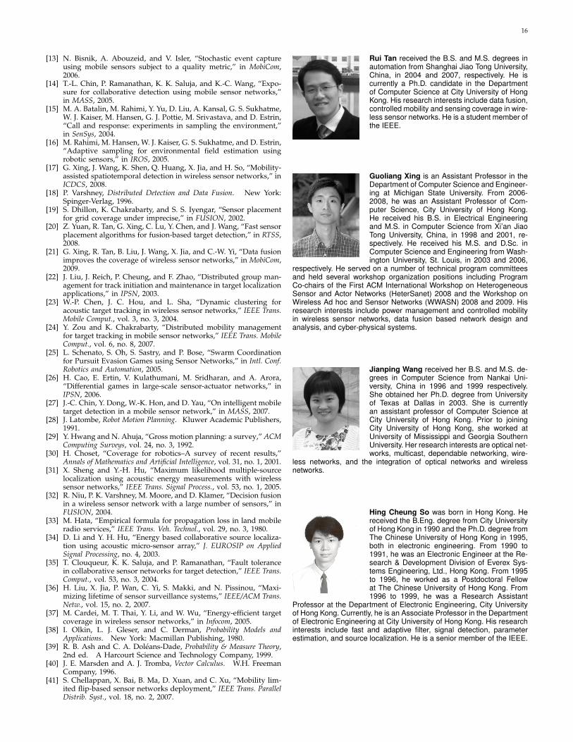
16
[13] N. Bisnik, A. Abouzeid, and V. Isler, “Stochastic event captureusing mobile sensors subject to a quality metric,” in MobiCom,2006.
[14] T.-L. Chin, P. Ramanathan, K. K. Saluja, and K.-C. Wang, “Expo-sure for collaborative detection using mobile sensor networks,”in MASS, 2005.
[15] M. A. Batalin, M. Rahimi, Y. Yu, D. Liu, A. Kansal, G. S. Sukhatme,W. J. Kaiser, M. Hansen, G. J. Pottie, M. Srivastava, and D. Estrin,“Call and response: experiments in sampling the environment,”in SenSys, 2004.
[16] M. Rahimi, M. Hansen, W. J. Kaiser, G. S. Sukhatme, and D. Estrin,“Adaptive sampling for environmental field estimation usingrobotic sensors,” in IROS, 2005.
[17] G. Xing, J. Wang, K. Shen, Q. Huang, X. Jia, and H. So, “Mobility-assisted spatiotemporal detection in wireless sensor networks,” inICDCS, 2008.
[18] P. Varshney, Distributed Detection and Data Fusion. New York:Spinger-Verlag, 1996.
[19] S. Dhillon, K. Chakrabarty, and S. S. Iyengar, “Sensor placementfor grid coverage under imprecise,” in FUSION, 2002.
[20] Z. Yuan, R. Tan, G. Xing, C. Lu, Y. Chen, and J. Wang, “Fast sensorplacement algorithms for fusion-based target detection,” in RTSS,2008.
[21] G. Xing, R. Tan, B. Liu, J. Wang, X. Jia, and C.-W. Yi, “Data fusionimproves the coverage of wireless sensor networks,” in MobiCom,2009.
[22] J. Liu, J. Reich, P. Cheung, and F. Zhao, “Distributed group man-agement for track initiation and maintenance in target localizationapplications,” in IPSN, 2003.
[23] W.-P. Chen, J. C. Hou, and L. Sha, “Dynamic clustering foracoustic target tracking in wireless sensor networks,” IEEE Trans.Mobile Comput., vol. 3, no. 3, 2004.
[24] Y. Zou and K. Chakrabarty, “Distributed mobility managementfor target tracking in mobile sensor networks,” IEEE Trans. MobileComput., vol. 6, no. 8, 2007.
[25] L. Schenato, S. Oh, S. Sastry, and P. Bose, “Swarm Coordinationfor Pursuit Evasion Games using Sensor Networks,” in Intl. Conf.Robotics and Automation, 2005.
[26] H. Cao, E. Ertin, V. Kulathumani, M. Sridharan, and A. Arora,“Differential games in large-scale sensor-actuator networks,” inIPSN, 2006.
[27] J.-C. Chin, Y. Dong, W.-K. Hon, and D. Yau, “On intelligent mobiletarget detection in a mobile sensor network,” in MASS, 2007.
[28] J. Latombe, Robot Motion Planning. Kluwer Academic Publishers,1991.
[29] Y. Hwang and N. Ahuja, “Gross motion planning: a survey,” ACMComputing Surveys, vol. 24, no. 3, 1992.
[30] H. Choset, “Coverage for robotics–A survey of recent results,”Annals of Mathematics and Artificial Intelligence, vol. 31, no. 1, 2001.
[31] X. Sheng and Y.-H. Hu, “Maximum likelihood multiple-sourcelocalization using acoustic energy measurements with wirelesssensor networks,” IEEE Trans. Signal Process., vol. 53, no. 1, 2005.
[32] R. Niu, P. K. Varshney, M. Moore, and D. Klamer, “Decision fusionin a wireless sensor network with a large number of sensors,” inFUSION, 2004.
[33] M. Hata, “Empirical formula for propagation loss in land mobileradio services,” IEEE Trans. Veh. Technol., vol. 29, no. 3, 1980.
[34] D. Li and Y. H. Hu, “Energy based collaborative source localiza-tion using acoustic micro-sensor array,” J. EUROSIP on AppliedSignal Processing, no. 4, 2003.
[35] T. Clouqueur, K. K. Saluja, and P. Ramanathan, “Fault tolerancein collaborative sensor networks for target detection,” IEEE Trans.Comput., vol. 53, no. 3, 2004.
[36] H. Liu, X. Jia, P. Wan, C. Yi, S. Makki, and N. Pissinou, “Maxi-mizing lifetime of sensor surveillance systems,” IEEE/ACM Trans.Netw., vol. 15, no. 2, 2007.
[37] M. Cardei, M. T. Thai, Y. Li, and W. Wu, “Energy-efficient targetcoverage in wireless sensor networks,” in Infocom, 2005.
[38] I. Olkin, L. J. Gleser, and C. Derman, Probability Models andApplications. New York: Macmillan Publishing, 1980.
[39] R. B. Ash and C. A. Doleans-Dade, Probability & Measure Theory,2nd ed. A Harcourt Science and Technology Company, 1999.
[40] J. E. Marsden and A. J. Tromba, Vector Calculus. W.H. FreemanCompany, 1996.
[41] S. Chellappan, X. Bai, B. Ma, D. Xuan, and C. Xu, “Mobility lim-ited flip-based sensor networks deployment,” IEEE Trans. ParallelDistrib. Syst., vol. 18, no. 2, 2007.
Rui Tan received the B.S. and M.S. degrees inautomation from Shanghai Jiao Tong University,China, in 2004 and 2007, respectively. He iscurrently a Ph.D. candidate in the Departmentof Computer Science at City University of HongKong. His research interests include data fusion,controlled mobility and sensing coverage in wire-less sensor networks. He is a student member ofthe IEEE.
Guoliang Xing is an Assistant Professor in theDepartment of Computer Science and Engineer-ing at Michigan State University. From 2006-2008, he was an Assistant Professor of Com-puter Science, City University of Hong Kong.He received his B.S. in Electrical Engineeringand M.S. in Computer Science from Xi’an JiaoTong University, China, in 1998 and 2001, re-spectively. He received his M.S. and D.Sc. inComputer Science and Engineering from Wash-ington University, St. Louis, in 2003 and 2006,
respectively. He served on a number of technical program committeesand held several workshop organization positions including ProgramCo-chairs of the First ACM International Workshop on HeterogeneousSensor and Actor Networks (HeterSanet) 2008 and the Workshop onWireless Ad hoc and Sensor Networks (WWASN) 2008 and 2009. Hisresearch interests include power management and controlled mobilityin wireless sensor networks, data fusion based network design andanalysis, and cyber-physical systems.
Jianping Wang received her B.S. and M.S. de-grees in Computer Science from Nankai Uni-versity, China in 1996 and 1999 respectively.She obtained her Ph.D. degree from Universityof Texas at Dallas in 2003. She is currentlyan assistant professor of Computer Science atCity University of Hong Kong. Prior to joiningCity University of Hong Kong, she worked atUniversity of Mississippi and Georgia SouthernUniversity. Her research interests are optical net-works, multicast, dependable networking, wire-
less networks, and the integration of optical networks and wirelessnetworks.
Hing Cheung So was born in Hong Kong. Hereceived the B.Eng. degree from City Universityof Hong Kong in 1990 and the Ph.D. degree fromThe Chinese University of Hong Kong in 1995,both in electronic engineering. From 1990 to1991, he was an Electronic Engineer at the Re-search & Development Division of Everex Sys-tems Engineering, Ltd., Hong Kong. From 1995to 1996, he worked as a Postdoctoral Fellowat The Chinese University of Hong Kong. From1996 to 1999, he was a Research Assistant
Professor at the Department of Electronic Engineering, City Universityof Hong Kong. Currently, he is an Associate Professor in the Departmentof Electronic Engineering at City University of Hong Kong. His researchinterests include fast and adaptive filter, signal detection, parameterestimation, and source localization. He is a senior member of the IEEE.
![Defending Grey Attacks by Exploiting Wavelet Analysis in ... › pdf › 1506.05247.pdf · Analysis in Collaborative Filtering Recommender Systems Zhihai Yang 1 ... et al. [19] proposed](https://img.pdfslide.net/doc/110x75/5f04afdf7e708231d40f34ad/defending-grey-attacks-by-exploiting-wavelet-analysis-in-a-pdf-a-150605247pdf.jpg)


![Exploiting Potential Citation Papers in Scholarly Paper ...kanmy/talks/JCDL13-Kaz-Ver2.pdf · Scholarly Paper Recommendation [Wang and Blei., KDD’11]: Collaborative topic regression](https://img.pdfslide.net/doc/110x75/6006b895502554211a65849e/exploiting-potential-citation-papers-in-scholarly-paper-kanmytalksjcdl13-kaz-ver2pdf.jpg)