Embed Size (px)
Citation preview

EXPLOITING TRANSMIT CHANNEL SIDE INFORMATION IN MIMO
WIRELESS SYSTEMS
A DISSERTATION
SUBMITTED TO THE DEPARTMENT OF ELECTRICAL ENGINEERING
AND THE COMMITTEE ON GRADUATE STUDIES
OF STANFORD UNIVERSITY
IN PARTIAL FULFILLMENT OF THE REQUIREMENTS
FOR THE DEGREE OF
DOCTOR OF PHILOSOPHY
Mai Hong Vu
July 2006

c© Copyright by Mai Hong Vu 2007
All Rights Reserved
ii

I certify that I have read this dissertation and that, in my opinion, it is fully adequate
in scope and quality as a dissertation for the degree of Doctor of Philosophy.
Arogyaswami J. Paulraj (Principal Adviser)
I certify that I have read this dissertation and that, in my opinion, it is fully adequate
in scope and quality as a dissertation for the degree of Doctor of Philosophy.
Stephen P. Boyd
I certify that I have read this dissertation and that, in my opinion, it is fully adequate
in scope and quality as a dissertation for the degree of Doctor of Philosophy.
John M. Cioffi
Approved for the University Committee on Graduate Studies.
iii

iv
Abstract
Transmit channel side information (CSIT) is information about the channel available to
the transmitter. In multiple-input multiple-output (MIMO) wireless, CSIT can signifi-
cantly improve system performance by increasing the transmission rate and enhancing
reliability. The time-varying nature of the wireless channel, however, often results in par-
tial CSIT. Partial information poses challenges to signal design to exploit the CSIT and
to performance analysis of the resulting system.
This thesis focuses on exploiting partial CSIT in a single-user MIMO wireless system,
assuming perfect channel knowledge at the receiver. The thesis approaches this problem
in three steps: building a dynamic CSIT model, deriving the capacity gains with CSIT,
and designing optimal precoding schemes to exploit the CSIT. The results are applicable
to practical MIMO wireless systems.
Due to inherent delays in CSIT acquisition, CSIT modeling must account for channel
temporal variation. A dynamic CSIT model is accordingly constructed, using an initial
channel measurement, the delay, and the channel statistics. The CSIT consists of a
channel estimate and its error covariance, which function as an effective channel mean
and covariance, respectively. Both parameters depend on the channel temporal correlation
factor, indicating the CSIT quality. Parameterizing by this factor, dynamic CSIT covers
the range from perfect channel estimate at zero delay to the actual channel mean and
covariance as the delay grows.
Dynamic CSIT multiplicatively increases the capacity at low signal-to-noise ratios
(SNRs) for all multi-input systems. The optimal input signal then is typically simple
single-mode beamforming. At high SNRs, dynamic CSIT can additively increase the
v

capacity for systems with more transmit than receive antennas. The optimal signal can
drop modes at high SNRs, depending on the CSIT. Furthermore, a convex optimization
program is developed to find the MIMO capacity given a dynamic CSIT. Using this
program, a simple, analytical capacity lower-bound, based on the Jensen-optimal input,
is shown to be tight in many cases.
Linear precoders can optimally exploit CSIT. A linear precoder functions as a multi-
mode beamformer, spatially directing signal and allocating power based on the CSIT.
A precoder is designed to exploit a dynamic CSIT in systems employing a space-time
block code. The design relies on a dynamic water-filling algorithm, in which both the
beam direction and power evolve with each water-filling iteration. The precoder achieves
a range of significant SNR gain and is robust to changing CSIT quality. Another pre-
coder is designed for high-K channels, given the CSIT as the channel amplitudes and the
channel phase-shift distribution. This CSIT helps simplify the precoder to single-mode
beamforming, with per-antenna power allocation dependent on the phase-shift distribu-
tion.
vi

Acknowledgments
My PhD study at Stanford University has been a journey of discovery and professional
growth. Having arrived where I am today, I owe thanks to many people.
First, I thank my advisor, Professor Arogyaswami J. Paulraj, for his guidance and
support throughout the years I worked with him. His engineering insights and technical
depth in wireless, together with the critical ability to connect theory to practice, have
been a source of inspiration. I am thankful for the opportunity to work with him and for
the cultivating time during my PhD.
Thanks to Professors Stephen Boyd for his stimulating classes, and for the masterfully-
written and easy-to-understand book on convex optimization. From them, I have learned
convex optimization theory and applied it extensively in my research.
Thanks to Professor John Cioffi for the challenging, yet essential, digital communi-
cation classes. I am grateful for his taking the time and providing valuable advices on
occasions I spoke to him. I am also thankful for his kindly letting me attend his weekly
group meetings during the last year, which I enjoyed and learned a lot from.
Thanks to Professor George Papanicolaous for being particularly supportive, and for
the stimulating discussions during the time-reversal and smart-antenna groups meetings
over the last couple of years. His mathematical insights and curiosity have always been
encouraging.
I thank Professor Mark Horowitz for his mentoring and unwavering support during
my first few years at Stanford. It had been a privilege working with him.
I enjoyed the intellectual environment Stanford harbors and appreciate the interac-
tions with other students and researchers. To this aspect, I must thank SARG members
vii

for being dynamic colleagues and for creating a stimulating research environment.
During my time at Stanford, I have also had the opportunities to know and interact
with many other people, who have enriched and made unique my experience. Thanks
especially to the friendly administrative staff who helped make things go smoothly: Kath-
leen Kimpo, Dennis Murphy, Pat Oshiro, Kelly Yilmaz, and Diane Shankle.
I would like to acknowledge the financial support of the Electrical Engineering Diver-
sity PhD Fellowship, the Rambus Stanford Graduate Fellowship, and the Intel Foundation
PhD Fellowship. These fellowships have enabled my PhD education and allowed me the
opportunities to explore and define my research areas.
Last but not least, I thank my family for their constant support and encouragements.
My journey so far would not have been possible without their love and support.
viii

Contents
Abstract v
Acknowledgments vii
1 INTRODUCTION 1
1.1 Benefits of transmit channel side information . . . . . . . . . . . . . . . . 3
1.2 Foundation for exploiting CSIT . . . . . . . . . . . . . . . . . . . . . . . . 4
1.3 Function of a linear precoder . . . . . . . . . . . . . . . . . . . . . . . . . 6
1.4 Thesis contribution . . . . . . . . . . . . . . . . . . . . . . . . . . . . . . . 8
1.4.1 Dynamic CSIT modeling . . . . . . . . . . . . . . . . . . . . . . . 8
1.4.2 Channel capacity and optimal input with CSIT . . . . . . . . . . . 9
1.4.3 Precoding designs exploiting CSIT . . . . . . . . . . . . . . . . . . 10
1.5 Thesis outline . . . . . . . . . . . . . . . . . . . . . . . . . . . . . . . . . . 11
2 TRANSMIT CHANNEL SIDE INFORMATION MODELS 13
2.1 The wireless channel . . . . . . . . . . . . . . . . . . . . . . . . . . . . . . 14
2.1.1 Multipath fading channel characteristics . . . . . . . . . . . . . . . 15
2.1.2 Statistical channel models . . . . . . . . . . . . . . . . . . . . . . . 20
2.2 MIMO channel parameters . . . . . . . . . . . . . . . . . . . . . . . . . . 22
2.2.1 The spatial dimension . . . . . . . . . . . . . . . . . . . . . . . . . 22
2.2.2 Channel covariance and antenna correlations . . . . . . . . . . . . 24
2.2.3 Channel mean and the Rician K factor . . . . . . . . . . . . . . . 25
2.2.4 Channel auto-covariance and the Doppler spread . . . . . . . . . . 26
ix

2.3 Transmit channel acquisition . . . . . . . . . . . . . . . . . . . . . . . . . 27
2.3.1 Reciprocity-based methods . . . . . . . . . . . . . . . . . . . . . . 27
2.3.2 Feedback-based methods . . . . . . . . . . . . . . . . . . . . . . . . 29
2.4 A dynamic CSIT model . . . . . . . . . . . . . . . . . . . . . . . . . . . . 30
2.4.1 MMSE channel estimation at the transmitter . . . . . . . . . . . . 31
2.4.2 Dynamic CSIT with homogeneous temporal correlation . . . . . . 32
2.4.3 Special CSIT cases . . . . . . . . . . . . . . . . . . . . . . . . . . . 33
2.5 A high-K variable-phase CSIT model . . . . . . . . . . . . . . . . . . . . . 34
2.6 Chapter summary . . . . . . . . . . . . . . . . . . . . . . . . . . . . . . . 35
3 MIMO CAPACITY WITH DYNAMIC CSIT 37
3.1 Channel ergodic capacity with dynamic CSIT . . . . . . . . . . . . . . . . 39
3.1.1 The ergodic capacity formulation . . . . . . . . . . . . . . . . . . . 39
3.1.2 The optimal input covariance . . . . . . . . . . . . . . . . . . . . . 40
3.2 Asymptotic-SNR capacity gains . . . . . . . . . . . . . . . . . . . . . . . . 42
3.2.1 Low-SNR optimal beamforming and capacity gain . . . . . . . . . 42
3.2.2 High-SNR capacity gain . . . . . . . . . . . . . . . . . . . . . . . . 46
3.3 Optimal input characterizations . . . . . . . . . . . . . . . . . . . . . . . . 50
3.3.1 Systems with equal or fewer transmit than receive antennas . . . . 51
3.3.2 Systems with more transmit than receive antennas . . . . . . . . . 51
3.4 Capacity optimization . . . . . . . . . . . . . . . . . . . . . . . . . . . . . 58
3.4.1 Convex optimization methods . . . . . . . . . . . . . . . . . . . . . 59
3.4.2 Optimization complexity and examples . . . . . . . . . . . . . . . 63
3.5 Capacity analysis using the optimization program . . . . . . . . . . . . . . 64
3.5.1 Channel capacity and the Jensen-optimal input covariance . . . . . 65
3.5.2 The capacity versus dynamic CSIT quality . . . . . . . . . . . . . 68
3.5.3 Effects of the K factor . . . . . . . . . . . . . . . . . . . . . . . . . 69
3.6 Chapter summary . . . . . . . . . . . . . . . . . . . . . . . . . . . . . . . 70
4 PRECODING SCHEMES EXPLOITING DYNAMIC CSIT 72
4.1 System configuration . . . . . . . . . . . . . . . . . . . . . . . . . . . . . . 74
x

4.2 Precoding design criteria . . . . . . . . . . . . . . . . . . . . . . . . . . . . 76
4.2.1 The pair-wise error probability measure . . . . . . . . . . . . . . . 77
4.2.2 The system capacity measure . . . . . . . . . . . . . . . . . . . . . 81
4.3 Optimal precoders based on the PEP per-distance . . . . . . . . . . . . . 82
4.3.1 Precoder design with orthogonal STBC . . . . . . . . . . . . . . . 83
4.3.2 Precoder design with general STBC . . . . . . . . . . . . . . . . . 90
4.3.3 Design examples and performance results . . . . . . . . . . . . . . 94
4.4 Analyses of PEP-based precoders . . . . . . . . . . . . . . . . . . . . . . . 100
4.4.1 The precoding gain . . . . . . . . . . . . . . . . . . . . . . . . . . . 100
4.4.2 Asymptotic precoder results . . . . . . . . . . . . . . . . . . . . . . 103
4.4.3 Special scenarios of the precoder design . . . . . . . . . . . . . . . 108
4.5 Precoders based on the system capacity . . . . . . . . . . . . . . . . . . . 112
4.5.1 The optimal input-shaping matrix . . . . . . . . . . . . . . . . . . 112
4.5.2 The optimal beam directions . . . . . . . . . . . . . . . . . . . . . 113
4.5.3 Power allocation . . . . . . . . . . . . . . . . . . . . . . . . . . . . 114
4.6 Precoding design comparison . . . . . . . . . . . . . . . . . . . . . . . . . 115
4.6.1 Structural similarities and differences . . . . . . . . . . . . . . . . 115
4.6.2 Performance comparison . . . . . . . . . . . . . . . . . . . . . . . . 116
4.6.3 Discussion on the precoding gain . . . . . . . . . . . . . . . . . . . 120
4.7 Chapter summary . . . . . . . . . . . . . . . . . . . . . . . . . . . . . . . 121
5 TRANSMISSION WITH HIGH-K VARIABLE-PHASE CSIT 123
5.1 Capacity maximization and result summary . . . . . . . . . . . . . . . . . 125
5.1.1 Ergodic capacity maximization . . . . . . . . . . . . . . . . . . . . 125
5.1.2 Summary of results . . . . . . . . . . . . . . . . . . . . . . . . . . . 128
5.2 The optimal signal phase-shift . . . . . . . . . . . . . . . . . . . . . . . . . 129
5.3 The optimal signal power and correlation . . . . . . . . . . . . . . . . . . 130
5.3.1 Unequal antenna gains . . . . . . . . . . . . . . . . . . . . . . . . . 130
5.3.2 Equal antenna gains . . . . . . . . . . . . . . . . . . . . . . . . . . 133
5.4 Design examples . . . . . . . . . . . . . . . . . . . . . . . . . . . . . . . . 135
5.4.1 Unequal antenna gains . . . . . . . . . . . . . . . . . . . . . . . . . 136
xi

5.4.2 Equal antenna gains . . . . . . . . . . . . . . . . . . . . . . . . . . 137
5.5 Benefits of high-K variable-phase CSIT . . . . . . . . . . . . . . . . . . . . 138
5.5.1 The capacity gain . . . . . . . . . . . . . . . . . . . . . . . . . . . 138
5.5.2 The simple transmission scheme . . . . . . . . . . . . . . . . . . . 140
5.6 Chapter summary . . . . . . . . . . . . . . . . . . . . . . . . . . . . . . . 141
6 CONCLUSION 142
6.1 Thesis summary . . . . . . . . . . . . . . . . . . . . . . . . . . . . . . . . 142
6.2 Precoding deployment in wireless standards . . . . . . . . . . . . . . . . . 144
6.3 Future directions . . . . . . . . . . . . . . . . . . . . . . . . . . . . . . . . 145
A Derivations and Proofs 147
A.1 K-factor threshold for mode-dropping at all SNRs . . . . . . . . . . . . . 147
A.2 Rt condition-number threshold for mode-dropping at all SNRs . . . . . . 148
A.3 Solving a quadratic matrix equation . . . . . . . . . . . . . . . . . . . . . 149
A.4 Deriving the bounds on ν in the outer algorithm . . . . . . . . . . . . . . 150
A.5 Solving the trace relaxation problem . . . . . . . . . . . . . . . . . . . . . 150
A.6 Optimal precoder with mean CSIT and non-identity A . . . . . . . . . . . 153
A.7 Optimal beam directions with transmit covariance CSIT . . . . . . . . . . 154
A.8 Optimal phase-shift with high-K variable-phase CSIT . . . . . . . . . . . 155
B Simulation Parameters 156
B.1 Channel parameter normalization . . . . . . . . . . . . . . . . . . . . . . . 156
B.2 Parameters for capacity optimization . . . . . . . . . . . . . . . . . . . . . 157
B.3 Parameters for precoding with dynamic CSIT . . . . . . . . . . . . . . . . 158
B.4 Parameters for precoding comparison . . . . . . . . . . . . . . . . . . . . . 159
Notation 160
Bibliography 163
xii

List of Figures
1.1 Capacity of 4 × 2 channels with and without CSIT. . . . . . . . . . . . . . 3
1.2 Error performance of a 4 × 1 system with and without CSIT. . . . . . . . 4
1.3 An optimal configuration for exploiting CSIT in a MIMO fading channel. 5
1.4 A linear precoder as a beamformer. . . . . . . . . . . . . . . . . . . . . . . 6
1.5 Transmit radiation patterns without (a) and with (b) precoding, based
on four orthogonal eigen-beams. The outer-most line represents the total
radiation pattern, and other lines are the patterns of the four beams. . . . 7
2.1 Amplitude of the temporal channel response of two different scalar wireless
links. . . . . . . . . . . . . . . . . . . . . . . . . . . . . . . . . . . . . . . . 18
2.2 Single-path spatial propagation model. . . . . . . . . . . . . . . . . . . . . 23
2.3 Obtaining CSIT using reciprocity. . . . . . . . . . . . . . . . . . . . . . . 28
2.4 Obtaining CSIT using feedback. . . . . . . . . . . . . . . . . . . . . . . . . 29
2.5 Dynamic CSIT model in the form of a delay-dependent channel estimate
(bold vector) and its error covariance (shaded ellipse). . . . . . . . . . . . 33
2.6 The Rician phase distribution. . . . . . . . . . . . . . . . . . . . . . . . . 35
3.1 Ratio of the capacity of i.i.d. channels with perfect CSIT to that without
CSIT. The legend denotes the numbers of transmit and receive antennas.
The asymptotic capacity ratio, in the limit of large number of antennas,
while keeping the number of transmit antennas twice the receive, is 5.83. . 45
3.2 Incremental capacity gain from perfect CSIT for i.i.d. channels. The legend
denotes the numbers of transmit and receive antennas. . . . . . . . . . . . 48
xiii
3.3 Capacity of channels with rank-one transmit correlation at SNR = 10dB,
without and with transmit covariance CSIT. . . . . . . . . . . . . . . . . . 50
3.4 K factor thresholds for systems with 2 receive and more than 2 transmit
antennas, above which using 2 modes is capacity-optimal for the mean
CSIT (3.15) at all SNRs. . . . . . . . . . . . . . . . . . . . . . . . . . . . . 55
3.5 Input power allocations for a 4×2 zero-mean channel with transmit covari-
ance eigenvalues [1.25 1.25 1.25 0.25]. Each allocation scheme contains
4 power levels, corresponding to the 4 eigen-modes of the transmit covari-
ance. The optimal allocation has 3 equal modes, as does the Jensen power
at low SNRs. The fourth mode of the optimal scheme always has zero power. 58
3.6 Optimization runtime complexity versus (a) the number of channel samples
(at N = M = 4) and (b) the number of antennas (N = M , at 10000 samples). 63
3.7 An optimization example of finding the ergodic capacity of a 4× 2 channel
at SNR = 10dB, using 20000 independently generated channel samples
in each iteration. The optimization and channel parameters are given in
Appendix B.2. (a) Mutual information value (nats/sec/Hz); (b) Its gap-
to-optimal. . . . . . . . . . . . . . . . . . . . . . . . . . . . . . . . . . . . 64
3.8 Capacity and mutual information of (a) a 4× 4 system, (c) a 4× 2 system;
with the corresponding power allocations in (b) and (d). The channel mean
and transmit covariance are specified in Appendix B.2. . . . . . . . . . . . 67
3.9 Ergodic capacity versus the CSIT quality ρ at SNR = 4dB. . . . . . . . . 68
3.10 Ergodic capacity and mutual information versus the K factor. . . . . . . . 69
3.11 K factor threshold for the 4×2 channels for tight lower-bound of the ergodic
capacity by the Jensen mutual information (difference < 0.03 bps/Hz). . . 70
4.1 Configuration of a system with linear precoder. . . . . . . . . . . . . . . . 75
4.2 Performance of a 2 × 1 system with and without precoding, using the
Alamouti code and (a) QPSK modulation, (b) various QAMs. . . . . . . . 96
4.3 Performance of a 4 × 1 system with and without precoding, using the
QSTBC and (a) QPSK modulation, (b) 16 QAM. . . . . . . . . . . . . . . 98
xiv

4.4 Performance of the minimum-distance PEP precoder in a 4×1 system with
OSTBC, given dynamic CSIT. . . . . . . . . . . . . . . . . . . . . . . . . 99
4.5 Performance comparison between the minimum-distance PEP precoder
and the beamforming scheme relying only on outdated channel measure-
ments. . . . . . . . . . . . . . . . . . . . . . . . . . . . . . . . . . . . . . . 100
4.6 Single-mode and multi-mode beamforming regions of the precoder for a
2 × 1 system. . . . . . . . . . . . . . . . . . . . . . . . . . . . . . . . . . . 108
4.7 Simulation system configuration. . . . . . . . . . . . . . . . . . . . . . . . 116
4.8 Comparative precoding performance with perfect CSIT: (a) uncoded; (b)
coded. . . . . . . . . . . . . . . . . . . . . . . . . . . . . . . . . . . . . . . 117
4.9 Comparative precoding performance with transmit covariance CSIT: (a)
uncoded; (b) coded. . . . . . . . . . . . . . . . . . . . . . . . . . . . . . . 119
4.10 System performance with dynamic CSIT using the minimum-distance PEP
precoder: (a) uncoded; (b) coded. . . . . . . . . . . . . . . . . . . . . . . . 120
4.11 Regions of different numbers of beams of the minimum-distance PEP pre-
coder for a 4 × 2 system. . . . . . . . . . . . . . . . . . . . . . . . . . . . . 121
5.1 A 2 × 1 system with high-K variable-phase CSIT. . . . . . . . . . . . . . . 125
5.2 The optimal power allocation η? with unequal antenna gains (SNR = 10dB).136
5.3 Slices of the optimal η? with unequal antenna gains. . . . . . . . . . . . . 137
5.4 The optimal signal correlation %? with equal antenna gains. . . . . . . . . 138
5.5 The optimal power allocation η? with equal antenna gains. . . . . . . . . . 139
5.6 Capacity with various channel knowledge. . . . . . . . . . . . . . . . . . . 140
xv

xvi

Chapter 1
INTRODUCTION
During the last decade, wireless communication has enjoyed tremendous growth in both
voice and data appliances. Cell phones and laptops with wireless capability are becoming
increasingly common. Not only the voice quality of cell phones has been improving, the
data rate of wireless LANs has also reached unprecedented levels of hundreds of megabits
per seconds [1, 2], allowing seamless connectivity. New capabilities are being realized,
such as providing broadband voice and data on a single unit [3], video broadcasting on
cell phones [4], and replacing cables with high-speed wireless connectors [5].
One of the technological enablers of such advances, and a breakthrough in wireless
technology, is the use of multiple antennas at both the transmitter and the receiver.
Multiple-input multiple-output (MIMO) systems allow a growth in transmission rate lin-
ear in the minimum of the numbers of antennas at each end [6]. They also enhance link
reliability and improve coverage [7]. MIMO is now entering next generation cellular and
wireless LAN products [2, 3, 8], with the promise of widespread adoption in the near
future.
While the benefits of MIMO are realizable when the receiver alone knows the com-
munication channel, these are further enhanced when the transmitter also knows the
channel. The value of transmit channel knowledge can be significant. For example, in a
4-transmit 2-receive antenna system, transmit channel knowledge can more than double
the capacity at −5dB SNR and add 1.5bps/Hz to the capacity at 5dB SNR. Such SNR
ranges are common in practical wireless systems. Therefore, exploiting transmit channel
1

2 CHAPTER 1. INTRODUCTION
side information (CSIT) in MIMO wireless is of great practical interest.
The random time-varying wireless medium, however, makes it difficult and often ex-
pensive to obtain perfect CSIT. In closed-loop methods, CSIT is degraded by the limited
feedback resources, associated feedback delays, and scheduling lags, especially for mobile
users with a small channel coherence time [9]. In open-loop methods, antenna calibration
errors and turn-around time lags again limit CSIT accuracy [10]. Therefore, the trans-
mitter often only has partial channel information. Schemes exploiting partial CSIT thus
are both important and necessary.
This thesis focuses on modeling partial CSIT, analyzing capacity benefits of the CSIT,
and designing schemes to exploit it. A major challenge in modeling CSIT is capturing
the channel time-variation. Due to delays in acquiring channel information, this time-
variation directly affects the CSIT quality and results in partial information. Nevertheless,
partial CSIT can still increase the channel capacity significantly. The capacity gain from
CSIT is subsequently quantified. To realize this gain, a transmit processing technique
called precoding, which operates on the signal before transmitting from the antennas,
can be used. For many common forms of partial CSIT, a linear precoder is optimal from
an information theoretic viewpoint [11, 12, 13]. A linear precoder functions as a multi-
mode beamformer, which optimally matches the input signal on one side to the channel
on the other side. It decouples the transmit signal into orthogonal spatial eigen-beams
and sends higher power along the beams where the channel is strong, but reduced or no
power along the weak, thus enhancing system performance.
In this introduction, the benefits of transmit channel side information are first dis-
cussed with concrete examples. A review follows on the information-theoretic foundation
for exploiting CSIT, establishing the optimality of linear precoders. The function of a lin-
ear precoder is then analyzed. These discussions form the foundation on which this thesis
is built. The thesis contribution is then concisely described. The last section outlines the
focus of each chapter in the thesis.

1.1. BENEFITS OF TRANSMIT CHANNEL SIDE INFORMATION 3
−5 0 5 10 15 200
2
4
6
8
10
12
14
16
SNR in dB
Erg
odic
cap
acity
(bi
ts/s
ec/H
z)
1.92 bps/Hz
1.97 bps/Hz
CSIT doubles
capacity
I.i.d no CSITI.i.d perfect CSITCorr. with CSITCorr. no CSIT
Figure 1.1: Capacity of 4 × 2 channels with and without CSIT.
1.1 Benefits of transmit channel side information
A wireless channel exhibits time, frequency, and space selective variations, known as
fading. This fading arises due to Doppler, delay, and angle spreads in the scattering
environment [14, 15, 7]. This thesis focuses on the time-varying channel, assuming fre-
quency flat and negligible angle spread. A frequency-flat solution, however, can be applied
per sub-carrier in a frequency-selective channel deploying orthogonal frequency-division
modulation (OFDM).
In a frequency-flat MIMO system, channel information can contain two dimensions:
temporal and spatial. Temporal CSIT – channel information across multiple time in-
stances – provides negligible capacity gain at medium-to-high SNRs [16]. Spatial CSIT,
which is channel information across antennas, on the other hand, offers potentially sig-
nificant increase in channel capacity at all SNRs. Figure 1.1 provides an example of this
capacity increase for two 4 × 2 channels. For the i.i.d channel, capacities with perfect
CSIT and without are plotted. For the correlated channel with rank-one transmit covari-
ance, capacities with the covariance knowledge and without are shown. The capacity gain
from CSIT at high SNRs here is significant, reaching almost 2 bps/Hz at 15 dB SNR.
At lower SNRs, although the absolute gain is not as high, the relative gain is much more
pronounced. For both channels, CSIT helps to double the capacity at −5 dB SNR.

4 CHAPTER 1. INTRODUCTION
−4 −2 0 2 4 6 8 10 12 14
10−5
10−4
10−3
10−2
10−1
100
SNR in dB
BE
R
6 dB
1/20
No CSITPerfect CSIT
Figure 1.2: Error performance of a 4 × 1 system with and without CSIT.
Spatial CSIT helps to not only increase capacity but also enhance system reliability
and reduce receiver complexity. Reliability can be measured by the system error per-
formance at a fixed transmission rate. By exploiting spatial CSIT, the error rate can
significantly decrease at the same SNR. Viewing it another way, the system can achieve
the same reliability with less transmit power. Figure 1.2 provides an example of such an
SNR gain in a 4× 1 system using QPSK. Without CSIT, the system employs an orthog-
onal space-time block code [17], while with perfect CSIT, it performs beamforming. At
10−3 bit error probability, the CSIT provides 6dB gain in SNR, implying reduced transmit
power by a factor of 4. Alternatively, at 7dB received SNR, the CSIT helps lower the error
probability 20 times. The next section explores the foundation for optimal processing to
exploit CSIT.
1.2 Foundation for exploiting CSIT
This section reviews the information theory background for a fading channel with causal
side information. The theory can be established by first examining a scalar channel [11].
Consider a frequency-flat time-varying channel h(s) with causal channel-state information
Us at the transmitter and perfect at the receiver, where s denotes the state. Given the
current CSIT Us, the channel h(s) is assumed to be independent of the past U s−11 =

1.2. FOUNDATION FOR EXPLOITING CSIT 5
NW^
i.i.d.Gaussian
CSIT
Transmitter
FPrecoder
EncoderC XW Channel
HY
Decoder
Figure 1.3: An optimal configuration for exploiting CSIT in a MIMO fading channel.
{U1, U2, . . . Us−1}:Pr (h(s)|U s
1 ) = Pr (h(s)|Us) . (1.1)
This condition enables the channel capacity to be a stationary function of the CSIT and
not depend on the entire CSIT history. The receiver is assumed to know how the CSIT is
used. The channel capacity with an average input power constraint E[|Xs|2] ≤ P is then
C = maxf
E
[
1
2log
(
1 + hf(U))
]
, (1.2)
where the expectation is over the joint distribution of h and U , and f(U) is a power
allocation function satisfying the constraint E[f(U)] ≤ P .
This result implies that it is capacity-optimal to separate channel coding and the
CSIT-exploiting function. The capacity of a channel with CSIT can be achieved by a
single Gaussian codebook designed for the channel without CSIT, provided that the code-
symbol power is dynamically scaled by an appropriate CSIT-dependent function f(U).
The combination of this CSIT-dependent function and the channel creates an effective
channel, outside of which coding can be applied as if the transmitter had no channel
side-information. This insight, in fact, can be traced back to Shannon [12]. For the scalar
fading channel, the CSIT-exploiting function is simply dynamic power-allocation.
Subsequently, the result has been extended to the MIMO fading channel [13]. The
channel state H(s) is now a matrix, and the optimal CSIT-exploiting function becomes
a weighting matrix – a linear precoder. Specifically, the capacity-optimal input can now
be decomposed as
X = F(Us)C . (1.3)

6 CHAPTER 1. INTRODUCTION
XC
Σ
Σ
VFd2
d1
UF
u1
d1
u2
d2
Figure 1.4: A linear precoder as a beamformer.
Here, C is a codeword optimal for an i.i.d Rayleigh-fading MIMO channel without CSIT,
generated from a complex Gaussian distribution with zero-mean and an appropriate co-
variance P I. The CSIT-exploiting function F(Us) is a weighting matrix, which directs
signal and allocates power spatially. In other words, the capacity-achieving signal is zero-
mean Gaussian-distributed with the covariance FF∗. This optimal input configuration is
depicted in Figure 1.3.
These results establish important properties of capacity-optimal signaling for a fading
channel with CSIT. First, it is optimal to separate the CSIT-exploiting function and chan-
nel coding, the latter designed for the channel without CSIT. Second, a linear precoder
is optimal for exploiting CSIT. The separation and linearity properties are the guiding
principles for precoder designs in single-user MIMO systems.
1.3 Function of a linear precoder
A linear precoder functions as the combination of an input shaper and a multi-mode
beamformer with per-beam power allocation. Consider the singular value decomposition
of the precoder matrix
F = UFDV∗F . (1.4)

1.3. FUNCTION OF A LINEAR PRECODER 7
−1 −0.5 0 0.5 1−1
−0.8
−0.6
−0.4
−0.2
0
0.2
0.4
0.6
0.8
1
(a)
−1.5 −1 −0.5 0 0.5 1 1.5 2−1.5
−1
−0.5
0
0.5
1
1.5
2
(b)
Figure 1.5: Transmit radiation patterns without (a) and with (b) precoding, based onfour orthogonal eigen-beams. The outer-most line represents the total radiation pattern,and other lines are the patterns of the four beams.
The orthogonal beam directions (patterns) are the left singular vectors UF ; the beam
power-loadings are the squared singular values D2. The right singular vectors VF form
the input shaping matrix, combining the input symbols from the encoder to feed into each
beam. The structure is shown in Figure 1.4. The beam directions and power-loadings are
influenced by the CSIT, the design criterion, and often, the SNR.
To ensure a constant average sum-transmit-power from all antennas, the precoder
must satisfy the power constraint
tr(FF∗) = 1 . (1.5)
This condition presumes that the input codeword C has been normalized for power ac-
cordingly.
Essentially, a linear precoder has two effects: decoupling the input signal into orthog-
onal spatial eigen-beams, and allocating power over these beams, based on the CSIT.
If the precoded orthogonal eigen-beams match the channel eigen-directions (the eigen-
vectors of H(s)∗H(s)), there will be no interference among signals sent on these beams,
creating parallel channels and allowing transmission of independent signal streams. This

8 CHAPTER 1. INTRODUCTION
effect, however, requires perfect CSIT. With partial CSIT, the precoder performs its best
to approximately match its eigen-beams to the channel eigen-directions, reducing the
interference among these beams. This is the decoupling effect. Moreover, the precoder
allocates power on these beams. For orthogonal eigen-beams, if all the beams have equal
power, the radiation pattern of the transmit antenna array is isotropic, as in the ex-
ample on the left in Figure 1.5. If the beam powers are different, however, the overall
transmit radiation pattern will have a specific shape, as shown on the right in Figure
1.5. By allocating power, the precoder effectively creates a radiation pattern matched
to the channel, based on the CSIT, so that higher power is sent in the directions where
the channel is strong and reduced or no power in the weak. More transmit antennas will
increase the transmitter ability to finely shape the radiation pattern and, therefore, are
likely to deliver more precoding gain.
1.4 Thesis contribution
This section summarizes the contribution of this thesis. The thesis focuses on study-
ing channel side-information at the transmitter (CSIT), while assuming perfect channel
knowledge at the receiver. Its contribution can be divided into 3 parts: characterizing
types of channel information and building a dynamic CSIT model; optimizing for the
capacity and deriving the capacity gain and optimal input with the CSIT; and designing
optimal precoding schemes to realize the gain.
1.4.1 Dynamic CSIT modeling
A major challenge in wireless communication is the time-variation of the channel. This
time-variation creates difficulty in obtaining channel information, which is required for
best performance. While the channel can be measured directly at the receiver with
sufficient accuracy, the transmitter must obtain channel information indirectly, using
either reciprocity or feedback. In a time-varying channel, the delay involved in such a
process can degrade the information accuracy.

1.4. THESIS CONTRIBUTION 9
The first contribution is characterizing channel information and constructing a dy-
namic CSIT model, taking into account channel time-variation. The model relies on
stochastic processes and estimation theories. Derived from a potentially outdated chan-
nel measurement and the channel statistics, this dynamic CSIT consists of a channel
estimate and its error covariance, acting as the effective channel mean and covariance.
Both parameters depend on a temporal correlation factor, indicating the CSIT quality.
Depending on this quality, the model covers smoothly from perfect to statistical channel
information [18, 19]. Dynamic CSIT is applicable to all Gaussian random channels.
In characterizing channel information, the thesis also considers another CSIT model
for a channel with high K factor. The K factor measures the ratio of power in the fixed
and the random parts of the channel. For this high-K model, the channel amplitude is
known perfectly at the transmitter, but the phase is known only in distribution. This
model is fundamentally different from dynamic CSIT and can be applied, for example, to
channels with a direct line-of-sight between the transmitter and the receiver.
1.4.2 Channel capacity and optimal input with CSIT
The second contribution consists of two parts: asymptotic analyses of the capacity gains
and the optimal input given dynamic CSIT, and a numerical convex optimization program
to find the capacity. Using function analysis and random matrix theory, the analyses in
the first part show that dynamic CSIT often multiplicatively increases the capacity at
low SNRs for all MIMO systems. It can additively increase the capacity at high SNRs
for systems with more transmit than receive antennas [20, 21]. The optimal input also
depends on the SNR. At low SNRs, it typically becomes single-mode beamforming on
the dominant eigen-mode of the channel correlation matrix. At high SNRs, the optimal
input differs across antenna configurations. For systems with equal or fewer transmit than
receive antennas, it approaches equi-power. With more transmit than receive antennas,
however, the optimal input is highly dependent on the CSIT and can drop modes for
channels with a strong mean or strongly correlated transmit antennas [20].
In the second part, optimizing for the channel capacity given a CSIT is a stochastic
convex problem. While convexity allows efficient implementations, the stochastic nature

10 CHAPTER 1. INTRODUCTION
complicates the problem. Efficient techniques to calculate the gradient, Hessian, and
function values required for the optimization are specified [22]. The program is then
used to study MIMO capacity with dynamic CSIT and to evaluate a simple capacity
lower-bound, derived using the Jensen-optimal input. The bound is tight at all SNRs for
systems with equal or fewer transmit than receive antennas, and at low SNRs for others.
1.4.3 Precoding designs exploiting CSIT
The third contribution involves designing linear precoders to exploit CSIT, using convex
analysis and matrix algebra. The thesis proposes analytical precoder designs for two CSIT
models. The first design exploits dynamic CSIT in the form of a known channel mean
and a known transmit covariance. Design criteria are characterized based on fundamental
and practical measures. For the fundamental measure, the precoder aims to maximize
the capacity of a system with a given input code. The design is then generalized for other
criteria with stochastic objective functions [19]. For the practical measure, a precoder
operates in a system with a space-time block code and aims to minimize the pair-wise
codeword error probability [23]. This precoder is designed using a dynamic water-filling
algorithm, in which both the precoding beam directions and power allocation evolve with
water-filling iterations. Depending on the CSIT quality, these precoders achieve a range
of significant and robust SNR gains [18, 19].
Another design is for a channel with CSIT as the channel amplitude and the phase
distribution. This CSIT typically applies to a channel with high K-factor. A channel with
2 transmit and 1 receive antenna is studied specifically. The capacity-optimal transmission
scheme is simple single-mode beamforming on the mean of the channel phase-shift, with
variable antenna power allocation, depending on the phase knowledge [24]. When the
phase is perfectly known, the scheme converges to maximum-ratio-combining transmit
beamforming. When the phase is completely unknown, the scheme reduces to single
antenna transmission.

1.5. THESIS OUTLINE 11
1.5 Thesis outline
This thesis consists of 4 main chapters. These chapters follow the contributions outlined
above, with the third contribution discussed in two chapters. A brief outline of each
chapter is as follows.
Chapter 2 discusses the wireless channel characteristics and modeling, MIMO parame-
ters, and techniques for acquiring channel information at the transmitter. It then
establishes models of transmit channel side-information, including dynamic CSIT
and a variable-phase model for high-K channels.
Chapter 3 focuses on the channel capacity with dynamic CSIT. The chapter first analyzes
asymptotic capacity gains from dynamic CSIT and the optimal input at low and
high SNRs. Results are established separately for systems with more transmit than
receive antennas, and with fewer or equal. The chapter then establishes a convex
optimization program to find the channel capacity. This program is used to study
effects on the capacity of antenna configurations, the CSIT quality, and the K
factor, and to assess a simple, analytical capacity lower-bound.
Chapter 4 proposes precoding designs to exploit dynamic CSIT. Two design criteria
are studied: the pair-wise error probability (PEP) and the system capacity. The
chapter establishes a PEP-optimal precoder for a system with a space-time block
code, distinguishing between orthogonal and non-orthogonal codes. This precoder
is then analyzed in terms of the precoding gain, asymptotic behaviors, and special
cases. The chapter also briefly discusses other precoding designs based on the system
capacity and generalizes for stochastic objective functions involving an expectation
without a closed-form. Comparative precoding performance are discussed.
Chapter 5 examines the capacity-optimal transmission scheme with high-K variable-
phase CSIT in a 2 × 1 system. The optimal scheme is simple beamforming, which
is established in terms of the signal phase and amplitude separately. The chapter
then discusses benefits of this CSIT, including the capacity gain and the simple
transmission scheme.

12 CHAPTER 1. INTRODUCTION
The last chapter, Chapter 6, provides the conclusion. This chapter summarizes the
main results of the thesis, discusses the deployment of precoding in emerging wireless
standards, and outlines future research directions.

Chapter 2
TRANSMIT CHANNEL SIDE
INFORMATION MODELS
The wireless channel is a multipath time-varying channel. The multiple paths arise from
signals reflecting off multiple random scatterers in the propagation environment. These
paths combine sometimes constructively and sometimes destructively, creating a channel
with multi-tap impulse response, in which each tap has a random phase and a time-varying
amplitude. The wireless channel is therefore often characterized statistically. The chan-
nel amplitude fluctuation is called fading, which occurs in both the time and frequency
domains. This chapter first establishes a model for the multipath fading channel, then
focuses on the frequency-flat case with single response tap.
Multiple antennas bring an additional spatial dimension. Each tap in the MIMO
channel is often represented as a matrix, containing multiple elements from the pairs
of transmit and receive antennas. These spatial elements can have different statistical
parameters. Their statistics characterize antenna correlation, channel mean, and spatial-
temporal auto-correlations. Spatial channel information, either instantaneous or statis-
tical, can bring significant improvement in system performance, such as increasing the
transmission rate and enhancing reliability.
Due to random fading, acquiring wireless channel information can be difficult. Chan-
nel acquisition at the receiver is usually aided by embedded pilots and therefore produces
13

14 CHAPTER 2. TRANSMIT CHANNEL SIDE INFORMATION MODELS
accurate information. Acquisition at the transmitter, however, has to rely on channel
measurements at a receiver, based on reciprocity or feedback. Both methods induce a
delay, causing potential loss in information accuracy. Assuming perfect channel knowl-
edge at the receiver, the chapter discusses transmit channel acquisition and characterizes
types of channel side information at the transmitter (CSIT).
This chapter introduces two spatial CSIT models. Dynamic CSIT includes a channel
estimate with known error covariance, based on an initial channel measurement and the
channel temporal and spatial statistics. This model applies to Gaussian random channels,
including both Rayleigh and Rician fading, and covers smoothly from statistical to perfect
channel knowledge. High-K variable-phase CSIT includes the channel amplitude and the
distribution of the channel phase-shift, applied specifically to 2 × 1 channels, typically
with a line-of-sight propagation path. These two models form the foundation for signal
design and system analysis in the subsequent chapters.
The chapter is organized as follows. The next section discusses the multipath fading
channel characteristics and establishes statistical channel models. Section 2.2 examines
the spatial dimension in MIMO and corresponding channel parameters. Transmit channel
acquisition principles and techniques are discussed in Section 2.3. The last two sections
present the two CSIT models, dynamic and high-K variable-phase, respectively.
2.1 The wireless channel
A wireless channel is created by wave propagation through multiple paths, arisen from
scattering, reflection, refraction, or diffraction of the radiated energy off objects in the
environment. The channel is often characterized on two different scales: large and small.
Large scale propagation captures path loss and shadowing, which result from signal at-
tenuation with distance and random blockage by large objects, such as hills and buildings.
Small scale propagation captures the variation arising from signals of random multiple
paths adding constructively and destructively. Such random variations create fading: sig-
nal strength fluctuation over all time, frequency, and space dimensions. Signal processing
for wireless communication usually exploits the small scale channel variation, also called

2.1. THE WIRELESS CHANNEL 15
multipath fading. Hence, this section focuses on the small-scale channel characteristics
and models, leaving the large-scale characteristics to references such as [15].
2.1.1 Multipath fading channel characteristics
Multipath fading arises from the sometimes constructive and sometimes destructive ad-
dition of signals arriving from multiple paths. Such fluctuation is caused by the random
scatterers in the wireless environment; it is intensified in mobile communications with
moving transmitter or receiver (or both). This section constructs the multipath fading-
channel impulse-response and studies its characteristics. These will form the basis for
establishing channel models in the next section.
The channel impulse response
When an ideal impulse is transmitted over a multipath fading channel, there will be two
effects on the received signal. First, since different signal paths may have different lengths
and attenuation factors, the received signal may appear as a train of pulses with differ-
ent delays and magnitudes. Second, due to the random nature of the wireless channel,
the multipath is varying with time. Thus the number of arrived pulses, the delay be-
tween them, and their magnitudes may vary each time sending the impulse. The impulse
response of the channel captures both of these effects, and is constructed as follows [25].
Consider transmitting a modulated signal, generally represented as
q(t) = Re[
x(t)ej2πfct]
(2.1)
where t is the continuous time, fc is the carrier frequency, and x(t) is the lowpass
information-carrying signal. Assuming that there are multiple propagation paths indexed
by k, each with a propagation delay τk(t) and an attenuation factor αk(t), which are both
time-varying, the received bandpass signal without noise may be expressed as
r(t) =K
∑
k=1
αk(t)q(
t − τk(t))
(2.2)

16 CHAPTER 2. TRANSMIT CHANNEL SIDE INFORMATION MODELS
where K is the total number of paths. Substituting x(t) in (2.1) yields
r(t) = Re{[
K∑
k=1
αk(t)e−j2πfcτk(t)x
(
t − τk(t))
]
ej2πfct}
.
The equivalent lowpass received signal therefore is
y(t) =K
∑
k=1
αk(t)e−j2πfcτk(t)x
(
t − τk(t))
.
The equivalent lowpass channel can then be described by the time-varying impulse re-
sponse [25]
h(τ, t) =K
∑
k=1
αk(t)e−j2πfcτk(t)δ
(
t − τk(t))
=K
∑
k=1
αk(t)eθk(t)δ
(
t − τk(t))
(2.3)
where θk(t) = −2πfcτk(t) is a time-varying phase sequence.
The impulse response h(τ, t) represents the response of the channel at time t caused by
an impulse applied at time t− τ . The channel is completely characterized by the number
of multipath components K and the path variables: amplitude ak(t), delay τk(t), and
phase θk(t). These parameters change unpredictably with time and are often described
statistically. The received signal r(t) therefore is also random, and when there are a large
number of paths, the central limit theorem applies. This means r(t) may be modeled as
a complex-valued Gaussian random process. Thus the channel impulse response h(τ, t) is
a complex-valued Gaussian random process in the t variable. The statistical models are
described in more detail in the next section.
Large dynamic changes in the transmitting medium are required for the amplitude
αk(t) to change sufficiently to cause a significant change in the received signal. On the
other hand, the phase θk(t) will change by 2π radians whenever the delay τk(t) (or in effect
the path length) is changed by 1/fc, which is a small amount due to large carrier frequency.
Therefore θk(t) can change quite rapidly with relatively small motions of the medium.
This time variation of the phases {θk(t)} is the primary cause of fading phenomena in a
multipath channel. The randomly time-varying phases {θk(t)} associated with the vectors

2.1. THE WIRELESS CHANNEL 17
{αk(t)eθk(t)} at times result in the received vectors adding constructively or destructively.
This adding causes amplitude variation in the received signal, termed signal fading.
Discrete-time channel model
For digital signal processing, the signal is processed in the sampled domain, hence it is con-
venient and necessary to represent the channel in discrete-time for analysis. The Nyquist
sampling frequency at twice the maximum signal bandwidth allows perfect reconstruction
of the continuous signal from its samples. In wireless communications, the received signal
sometimes needs to be sampled at a slightly higher frequency than Nyquist because of
possible bandwidth expansion through the channel. This work will assume that an appro-
priate sampling frequency has been chosen. A single time-sample of the channel response
at a specific delay is called a channel tap. Depending on the sampling resolution, the
number of distinguishable channel taps L is often smaller than the number of multipaths
(L ≤ K). From (2.3), a discretized channel can be obtained as h[n; k], representing the
channel response at the discrete time n caused by a unit sampled input at time n − k:
h[n; k] =L
∑
k=1
ak[n]eθk[n]δ[
n − k]
=L
∑
k=1
hk[n]δ[
n − k]
, (2.4)
where hk[n] = ak[n]eθk[n] is the kth channel response tap, in which ak[n] and θk[n] are the
composite tap amplitude and phase respectively.
Temporal selectivity
A wireless channel can be selective, characterized by a varying channel response, in both
the time and frequency domains. The impulse response (2.4) can be used to describe
the channel in these domains. The time dimension n relates to the channel temporal
selectivity, while the delay dimension k captures the spectral selectivity.
Figure 2.1 provides an example of channel temporal selectivity for two scalar wireless
links between two distinct pairs of transmit and receive antennas. Not only these channel
amplitudes fluctuate over time, they can do so independently, given sufficient antenna
spacing.

18 CHAPTER 2. TRANSMIT CHANNEL SIDE INFORMATION MODELS
0 2 4 6 8 10 12 14 16−10
−8
−6
−4
−2
0
2
Time (sec)
Mag
nitu
de (
dB)
0 2 4 6 8 10 12 14 16
−16
−14
−12
−10
−8
−6
−4
−2
0
2
Time (sec)
Mag
nitu
de (
dB)
Figure 2.1: Amplitude of the temporal channel response of two different scalar wirelesslinks.
Temporal selectivity is caused by motion of the transmitter, the receiver, or the scat-
terers in the channel. These motions cause a transmitted single tone to be spread in
frequency at the receiver. This effect can be captured in the power spectrum of the
channel taps. To simplify the derivation, assume the taps are stationary and statistically
independent. The temporal auto-correlation of the kth tap can then be obtained as
ρk[m] = E[
hk[n]hk[n + m]∗]
, (2.5)
which depends only on the time difference m but not the absolute time (here (.)∗ denotes
complex conjugation). The tap power spectral response is the Fourier transform of this
auto-correlation
Sk(f) =∑
m
ρk[m]e−j2πfm .
The frequency range over which Sk(f) is non-zero indicates the Doppler spread of tap k.
The maximum frequency spread among all taps is the channel Doppler spread fd. The
temporal auto-correlation function (2.5), which specifies how fast the channel decorrelates
with time, in turn can be expressed in terms of the time interval and the Doppler spread.
A popular model for all taps is Clark’s spectrum (popularized by Jake [14]), which assumes
uniformly distributed scatterers on a circle around the antenna,
ρ[m] = J0(2πfdm∆t) , (2.6)

2.1. THE WIRELESS CHANNEL 19
where J0 is the zeroth order Bessel function of the first kind, and ∆t is the sampling
interval. For other propagation environments, the temporal auto-correlation is often
obtained empirically.
Higher mobility in a system commonly causes larger Doppler spread and faster chan-
nel time variation. In other words, larger Doppler is associated with higher temporal
selectivity. A measure of the temporal selectivity is the channel coherence time, defined
as the time interval over which the channel remains strongly correlated. The shorter the
coherence time, the faster the channel changes with time. Since the coherence time is a
statistically defined quantity, an approximate relation to the Doppler is
Tc =1
fd. (2.7)
In some texts, there exists a constant such as 2, 4, or 8 in front of fd in this relation;
but there no single agreed-number. The important property is the inverse-proportionality
between Tc and fd.
Spectral selectivity
Spectral selectivity, on the other hand, is caused by the presence of multipath, or multiple
channel taps indexed by k. It can be captured in the channel frequency response, by taking
the Fourier transform of the channel taps as
Hk(f) =∑
n
hk[n]e−j2πfn .
The channel frequency response is the sum of the phase-shifted response of each tap
H(f) =∑
k
Hk(f)ej2πfk . (2.8)
Because of these frequency-dependent phase shifts, this sum varies with frequency, causing
selectivity. The more taps or equivalently longer multipath delays, the more frequency
selective the channel becomes. An indicator of this selectivity is the delay spread, defined

20 CHAPTER 2. TRANSMIT CHANNEL SIDE INFORMATION MODELS
as the range of multipath spread in the channel
Tm = τmax − τmin , (2.9)
where τmax and τmin are the maximum and minimum multipath delays, respectively. The
channel coherence bandwidth Bc is accordingly defined as
Bc =1
Tm. (2.10)
Bc indicates approximately the frequency separation at which the channel behaves in-
dependently. In other words, two transmitted single tones separated by the channel
coherence bandwidth or more will be affected by the channel in significantly different
ways.
2.1.2 Statistical channel models
Because of the often unpredictable time-varying nature of a wireless channel, the channel
is modeled as a random process. The channel at a single time instance therefore is a
random variable. Consider a single channel tap hk[n] of the channel at time n from (2.4),
this tap is contributed by a number of multipaths as
hk[n] = ak[n]ejθk[n] =
Lk∑
i=1
αi[n]ejθi[n] ,
where αi[n] and θi[n] are the amplitude and phase of path i respectively, and Lk is the
total number of contributing paths. The phases of these paths vary rapidly with time
and are often modeled as independent uniform random variables in [0, 2π]. The sum of
such random-phase components, in which no path has the magnitude dominant compared
with all others, can be well approximated as a Gaussian random variable with zero mean
[26]. The Gaussian statistics of hk[n] can also be inferred from applying the central limit
theorem to this summation of multiple and statistically similar paths.

2.1. THE WIRELESS CHANNEL 21
Often, the complex channel tap is expressed in terms of its real and imaginary parts
hk[n] = hkR[n] + jhkI [n] , (2.11)
where both parts are Gaussian random variables with zero mean and equal variance.
The channel variance represents the average power gain in the channel. It can be shown
then, that the tap amplitude ak[n] has the Rayleigh distribution and the phase uniform
in [0, 2π] (see [27]). The Rayleigh distribution has been verified empirically to be a good
fit for many channels, especially when there are many scatterers in the environment and
no direct line-of-sight between the transmitter and the receiver. It also models well the
fast fading channel components.
When there is a direct line-of-sight or a cluster of strong paths, the channel may have
a non-zero mean (a DC component). The channel then is often modeled as having Rician
statistics. The Rician distribution arises from the phase of a constant phasor perturbed
by additive, random zero-mean complex Gaussian noise with equal variance on the real
and imaginary parts [28]. The channel line-of-sight in this case acts as the constant phasor
while the other multipaths contribute to the zero-mean Gaussian part. In a multi-tap
channel, the line-of-sight usually affects only one tap. The real and imaginary parts of
that tap (2.11) are now non-zero mean Gaussian random variables; their variances are
equal but the means need not be. Other channel taps are still zero-mean.
There are yet other statistical models for wireless channels, such as Nakagami, Suzuki,
Weibull [26], in addition to empirical models. While these models may be more accurate
for some channels, they are also more complicated to work with because of a larger number
of parameters. Since the Rayleigh and Rician models can well represent a majority of
channels to sufficient detail, subsequent analyses will mainly use these models.
The variance of a zero-mean channel tap represents its power gain. The power gain
of a multi-tap channel is captured in the power-delay profile. A common model for this
profile is the exponential model, in which the tap power follows an exponential function
with the exponent as the negative of the tap delay
E[
|hk[n]|2]
= p0e−jkτ0 ,

22 CHAPTER 2. TRANSMIT CHANNEL SIDE INFORMATION MODELS
where p0 and τ0 are constants. For analysis, the power gain of a scalar channel between a
single transmit and a single receive antennas is often normalized to 1, counting all taps.
For a frequency-flat channel with single time-response tap, that tap is normalized to have
a unit variance.
Another parameter is the distribution of the path delay sequence, which has been
modeled less extensively. Existing models include Poison distribution, Gilbert’s burst
noise, and a pseudo-Markov model [26]. The analysis in this thesis, however, will fo-
cus solely on the frequency-flat channel; hence this parameter has no affect and will be
omitted.
2.2 MIMO channel parameters
The MIMO wireless channel is created by using multiple antennas at both the transmitter
and the receiver. It generalizes the special cases of having a single antenna at only one
side: multiple input single output (MISO), and single input multiple output (SIMO). In
addition to spanning the temporal and spectral dimensions, a MIMO channel exhibits
a new spatial dimension across the antennas. The channel contains multiple elements
among the antennas and is often represented in a matrix form. These elements can
correlate and can have different mean (line-of-sight) values. Their composite temporal
and spectral responses are also more complex than the scalar case.
2.2.1 The spatial dimension
For simplicity, let’s first examine the frequency-flat MIMO channel. The channel has only
a single tap. This tap, however, contains multiple elements between all pairs of transmit-
receive antennas. In a system with N transmit and M receive antennas, the channel can
be represented as a matrix H of size M × N
H =
h11 h12 · · · h1N
h21 h22 · · · h2N
...
hM1 hM2 · · · hMN
, (2.12)

2.2. MIMO CHANNEL PARAMETERS 23
θ
d
h1
d sin θ
h2 = αh1ejφ
Figure 2.2: Single-path spatial propagation model.
in which hij is the scalar channel from transmit antenna j to receive antenna i. For
brevity, the time-dependent index [n] has been omitted.
Each channel element hij can have different amplitude and phase, caused by spatial
selectivity. The channels at the same time, same frequency but at different locations
can experience different fading. To understand the underlying spatial effect, consider a
signal arriving at a two-antenna array from a single direction. The corresponding channel,
depicted in Figure 2.2, contains two propagation paths to the two antennas, h1 and h2,
which differ by a gain ratio α and a phase shift φ as
h2 = αejφh1 . (2.13)
The difference in antenna gains (when α 6= 1) is caused by the antenna array structure
and the local scattering from the mounting structure (walls, rooftops) near the antennas.
Although dependent on the angle of signal arrival, α is much less sensitive to its changes
than is the phase shift φ. The phase shift results from the difference in distances that
the wave propagates to the antennas. It depends on the angle of arrival θ, the distance d
between the two antennas, and the carrier frequency fc, or the wavelength λc equivalently,
as
φ = 2πd
λcsin θ . (2.14)
Depending on the antenna distance relative to the wavelength, this phase shift can be
highly variable in response to a small change in the angle of arrival θ. For example,

24 CHAPTER 2. TRANSMIT CHANNEL SIDE INFORMATION MODELS
at a distance of tens of the wavelength, if θ is uniformly distributed in [−π/3, π/3], the
distribution of φ looks almost uniform in [−π, π]. A similar single-path model applies
to multiple transmit-antenna channels, in which θ is the angle of departure. A typical
MIMO channel has multiple propagation paths from multiple directions. The multipath
makes the phase shifts between the channel elements even more sensitive to changes in
the angles of arrival or departure, causing the spatial selectivity in the channel.
A frequency-selective MIMO channel contains multiple matrix taps at different de-
lays. Elements of different taps are often assumed to be independent. The tap-delay
scalar channel between every transmit-receive antenna pair can have the same power-
delay profile, except any difference in the non-zero-mean tap of a Rician channel.
Similar to a scalar channel, each element hij in a MIMO channel can be modeled as
a complex Gaussian random process. These elements, however, can correlate and have
different means. Decompose the channel (2.12) into a fixed part and a variable part as
H = Hm + H , (2.15)
where Hm is the complex channel mean, and H is a zero-mean complex Gaussian random
matrix.
2.2.2 Channel covariance and antenna correlations
The channel covariance captures the spatial correlation among all the transmit and receive
antennas. It is defined among all MN channel elements as a MN × MN matrix
R0 = E[
hh∗]
, (2.16)
where h = vec(
H)
, and (.)∗ denotes a conjugate transpose. R0 is a positive semi-
definite Hermitian matrix. Its diagonal elements represent the power gain of the MN
scalar channels, and the off-diagonal elements are the cross-coupling between these scalar
channels.
The covariance R0 is often assumed to have a simplified, separable Kronecker structure
[29]. The Kronecker model assumes that the covariance of the scalar channels seen from

2.2. MIMO CHANNEL PARAMETERS 25
all N transmit antennas to a single receive antenna (corresponding to a row of H) is the
same for any receive antenna (any row) and equals to Rt (N × N). Let hTi be row i of
H, then
Rt = E[
hih∗i
]
for any i. Similarly, the covariance of the scalar channels seen from a single transmit
antenna to all M receive antennas (corresponding to a column of H) is assumed to be the
same for any transmit antenna (any column) and equals to Rr (M ×M). That is, let hj
be column j of H, then
Rr = E[
hjh∗j
]
for any j. Both covariance matrices Rt and Rr are complex Hermitian positive semi-
definite. The channel covariance can now be decomposed as
R0 = RTt ⊗ Rr , (2.17)
where ⊗ denotes the Kronecker product [30]. The channel (2.15) can then be written as
H = Hm + R1/2r HwR
1/2t , (2.18)
where Hw is a M×N matrix with zero-mean unit-variance i.i.d complex Gaussian entries.
Here R1/2t is the unique square-root of Rt, such that R
1/2t R
1/2t = Rt; similarly for R
1/2r .
The Kronecker correlation model has been experimentally verified in indoor environ-
ments for up to 3×3 antenna configurations [31, 32], and in outdoor environments for up
to 8×8 configurations [33]. Other more general covariance structures have been proposed
in the literature [34, 35], in which the transmit covariances (Rt) corresponding to different
reference receive antennas are assumed to have the same eigenvectors, but not necessarily
the same eigenvalues; similarly for Rr.
2.2.3 Channel mean and the Rician K factor
The channel mean is the fixed component of the channel, usually corresponding to a line-
of-sight propagation path or a cluster of strong paths. The mean of a MIMO channel is

26 CHAPTER 2. TRANSMIT CHANNEL SIDE INFORMATION MODELS
a complex matrix Hm of size M × N obtained as
Hm = E[H] . (2.19)
The elements of the mean can have different amplitudes and arbitrary phase, caused by
the spatial effect analyzed in Section 2.2.1. The strength of a channel mean can be loosely
quantified by the Rician K factor. It is defined as the ratio of the power in the channel
mean and the average power in the channel variable component as
K =||Hm||2Ftr(R0)
, (2.20)
where ||.||F is the matrix Frobenius norm, and tr(.) is the trace of a matrix. The K
factor can take any real value between 0 and infinity. When K = 0, the channel has the
Rayleigh distribution. When K → ∞, the channel becomes deterministic. Measurements
of fixed broadband channels have shown that the K factor can have a wide range from 0
to up-to 30dB in practice, and it tends to decrease with increasing distance between the
transmitter and the receiver [36].
2.2.4 Channel auto-covariance and the Doppler spread
The channel auto-covariance characterizes how rapidly the channel decorrelates with time.
Assuming stationarity, the covariance between two channels samples H[n] and H[n + m]
(2.15) depends only on the time difference but not the absolute time
R[m] = E[
h[n]h[n + m]∗]
, (2.21)
where h denotes the vectorized version of the corresponding zero-mean part of the channel
matrix. When m = 0, this auto-covariance coincides with the channel covariance R0
(2.16); when m becomes large, it eventually decays to zero.
For a MIMO channel, the covariance R0 captures the spatial correlation among all
the transmit and receive antennas, while the auto-covariance at a non-zero delay R[m]
captures both channel spatial and temporal correlations. Based on the premise that the

2.3. TRANSMIT CHANNEL ACQUISITION 27
channel temporal statistics can be the same for all antenna pairs, it may be assumed that
the temporal correlation is homogeneous and identical for any channel element. Then,
the two correlation effects are separable, and the channel auto-covariance becomes their
product as
R[m] = ρ[m]R0 , (2.22)
where ρ[m] is the temporal correlation of a scalar channel (2.5). In other words, all the
MN scalar channels between the M transmit and N receive antennas have the same tem-
poral correlation function. This temporal correlation is a function of the time difference
m and the channel Doppler spread. Similar assumptions for MIMO temporal correlation
have also been used in constructing channel models and verifying measurement data in
[32, 35].
2.3 Transmit channel acquisition
In a communication system, the signal enters the channel after leaving the transmitter.
Therefore, a transmitter can only acquire channel information indirectly, based on the
information at a receiver. The receiver can estimate the channel directly from the channel-
modified received-signal, usually based on embedded pilots. The transmitter can then
obtain the information in two ways, based on the reciprocity principle and by using
feedback.
2.3.1 Reciprocity-based methods
The reciprocity principle in wireless states that the forward channel from an antenna
A to another antenna B is identical to the transpose of the reverse channel from B to
A. Reciprocity requires the forward and reverse channels to be at the same frequency,
the same time, and the same antenna locations. In a full-duplex system, this principle
suggests that the transmitter (at A) can obtain the forward channel (A to B) from the
reverse channel (B to A), which the receiver (at A) can measure, as illustrated in Figure
2.3.
In real full-duplex communications, however, the forward and reverse links cannot use

28 CHAPTER 2. TRANSMIT CHANNEL SIDE INFORMATION MODELS
A B
Transceiver Transceiver
H
H
B−>A
A−>B
Figure 2.3: Obtaining CSIT using reciprocity.
all identical frequency, time, and space instances. The reciprocity principle may still hold
approximately if the difference in any of these dimensions is relatively small, compared
to the channel variation across the referenced dimension. In the temporal dimension, this
condition implies that any time lag ∆t between the forward and reverse transmissions
must be much smaller than the channel coherence time Tc:
∆t ¿ Tc .
Similarly, any frequency offset ∆f must be much smaller than the channel coherence
bandwidth Bc (∆f ¿ Bc), and the antenna location differences on the two links must be
much smaller than the channel coherence distance Dc [7].
Practical channel acquisition based on reciprocity may be applicable in time-division-
duplex (TDD) systems. While TDD systems often have identical forward and reverse
frequency bands and antennas, there is a turn-around delay between the forward and
reverse links. Such delay must be negligible compared to the channel coherence time. In
a frequency-division-duplex (FDD) system, the temporal and spatial dimensions may be
identical, but the frequency offset between the forward and reverse links is usually much
larger than the channel coherence bandwidth, due to high carrier frequency. Therefore,
reciprocity is usually not applicable in FDD systems [10].
To reduce the turn-around delay in TDD systems, especially in fast-fading mobile
communication, channel sounding is sometimes used. Channel sounding uses a reverse-
link transmission specifically for channel measurement, in which the scheduled users send
a sounding (pilot) signal to help the base learn their channels. The sounding signals are
orthogonal among simultaneously scheduled users. The obtained channel information is
used for the very next transmission to those users.

2.3. TRANSMIT CHANNEL ACQUISITION 29
A BTransceiver Transceiver
H
Figure 2.4: Obtaining CSIT using feedback.
A complication in using reciprocity methods is that the principle only applies to the
radio channel between the antennas, while in practice, the “channel” is measured and
used at the baseband processor. Different transmit and receive RF hardware chains
hence become part of the forward and reverse channels. Since these chains have different
frequency transfer characteristics, reciprocity requires transmit-receive chain calibration.
During calibration, the difference in the frequency response between the two chains are
identified [37]. A digital equalizer is then built and incorporated into the baseband section
to make the two chains effectively identical. This equalizer usually requires high numerical
precision and accuracy. Calibration must be performed periodically to track the slow time
variations of the RF chains.
2.3.2 Feedback-based methods
Another method of obtaining channel information at the transmitter is using feedback
from the receiver of the forward link, depicted in Figure 2.4. The channel is measured at
the receiver at B during the forward transmission (A to B), then the information is sent
to the transmitter at A on the reverse link. Feedback is not limited by the reciprocity
requirements. However, the feedback delay ∆t between channel measurement at B and
its use by the transmitter at A can be a source of error, unless it is much smaller than
the channel coherence time:
∆t ¿ Tc .
Feedback can also be used to send channel statistics that change much slower in time
compared to the channel itself. In such cases, the delay requirement for valid feedback
can be relaxed significantly.
Channel acquisition using feedback can be applied in both TDD and FDD systems,

30 CHAPTER 2. TRANSMIT CHANNEL SIDE INFORMATION MODELS
but is more common in FDD. Although not subjected to transmit-receive calibration,
feedback imposes another system overhead by using transmission resources. Therefore,
methods of reducing feedback overhead, such as quantizing feedback information, are of
practical importance [38, 39, 40]. These methods, however, are not a focus of this thesis.
2.4 A dynamic CSIT model
This section establishes a CSIT model in the form of a channel estimate and its error
covariance at the transmit time n. Although CSIT formulation as a noisy channel estimate
has been used in the literature [41, 42], this model is an explicit construction, using an
initial channel measurement and relevant channel statistics – mean, covariance, and auto-
correlation. The model applies to frequency-flat MIMO channels.
With both CSIT acquisition methods outlined in Section 2.3, there exists a delay from
when the channel information is measured to when it is used by the transmitter. Because
of the channel temporal variation, this delay may affect the reliability of the obtained
information, depending on the type of information. Consider instantaneous channel mea-
surements and the channel statistics. Instantaneous measurements are sensitive to the
delay, especially in mobile communication, leading to a potential mismatch between the
measurement and the channel at the time of use. Channel statistics, including the channel
mean (2.19), covariance (2.16) and auto-correlation (2.21), can be obtained by averaging
instantaneous measurements over tens of coherence times. They remain valid for tens to
hundreds coherence intervals, relatively long compared to a transmission interval. There-
fore, these statistics are not affected by channel acquisition delay and can be considered
reliable.
A more reliable and complete CSIT can provide more gain in system capacity and
performance. This principle suggests combining both instantaneous measurements and
the channel statistics to create a CSIT model robust to channel variation, while optimally
capturing the potential gain.

2.4. A DYNAMIC CSIT MODEL 31
2.4.1 MMSE channel estimation at the transmitter
Suppose that the transmitter has an initial channel measurement at time 0 and relevant
channel statistics. Consider CSIT at the transmit time n in the form of a channel estimate
and its error covariance. The main source of irreducible error in channel estimation is
the random channel time-variation. Thus, assume the channel measurement at time 0
error-free, the error in the channel estimate depends only on the delay n between this
initial measurement and its use by the transmitter.
Denote H[n] as the channel estimate at time n, and E[n] as the estimation error with
correlation Re[n]. A CSIT model can then be written as
H[n] = H[n] + E[n] ,
Re[n] = E[
e[n]e[n]∗]
.(2.23)
where e[n] = vec(
E[n])
. Assuming unbiased estimates, E[n] can be modeled as a station-
ary zero-mean Gaussian random process. Re[n] is then the error covariance dependent
on the delay n and the Doppler spread. The CSIT consists of the estimate H[n] and its
error covariance Re[n]. At time zero, E[0] = 0 and Re[0] = 0, corresponding to perfect
CSIT.
Assume that the initial channel measurement H[0] with the channel statistics Hm,
R0, and R[n] are available to the transmitter. Then the CSIT at time n follows from the
MMSE estimation theory [43] as
h[n] = E[
h[n]|h[0]]
= hm + R[n]∗R−10 (h[0] − hm)
Re[n] = cov[
h[n]|h[0]]
= R0 − R[n]∗R−10 R[n] ,
(2.24)
where h[n] = vec(
H[n])
(note that the lower-case letters h denote the vectorized version
of the corresponding upper-case matrices H). A similar method was used for estimating
a scalar time-varying channel from a vector of outdated estimates [44]. The channel
estimate with error covariance (2.24) is an explicit construction of the CSIT model as a
noisy channel estimate for a MIMO system.
The two quantities {H[n],Re[n]} constitutes the CSIT. They effectively function as a

32 CHAPTER 2. TRANSMIT CHANNEL SIDE INFORMATION MODELS
channel mean and a channel covariance at a delay n. Thus H and Re are also referred to
as the effective mean and effective covariance, respectively, and the pair forms an effective
statistics.
2.4.2 Dynamic CSIT with homogeneous temporal correlation
Using the homogeneous channel temporal-correlation model (2.22), the channel estimate
and its error covariance become
H[n] = ρ[n]H0 + (1 − ρ[n])Hm ,
Re[n] =(
1 − ρ[n]2)
R0 .(2.25)
The CSIT can now be simply characterized as a function of ρ[n], the initial channel
measurement H0, and the channel mean Hm and covariance R0. The channel estimate
becomes a linear combination of the initial measurement and the channel mean. The error
covariance is a linear function of the channel covariance alone. With Kronecker antenna
correlation (2.17), the estimated channel has the effective antenna correlations as
Rt,e[n] =√
1 − ρ[n]2 Rt ,
Rr,e[n] =√
1 − ρ[n]2 Rr ,(2.26)
which again follow a Kronecker structure. When the antennas at the receiver are uncor-
related, Rr = I, then the effective receive correlation is assumed to be Rr,e[n] = I, and
the effective transmit correlation becomes
Rt,e[n] =(
1 − ρ[n]2)
Rt . (2.27)
In the CSIT models (2.25) and (2.26), ρ[n] acts as a channel estimate quality depen-
dent on the time delay n. For a zero or short delay, ρ is close to 1; the estimate depends
heavily on the initial channel measurement, and the error covariance is small. As the delay
increases, ρ decreases in magnitude to 0, reducing the impact of the initial measurement.
The estimate then moves toward the channel mean Hm, and the error covariance grows
toward the channel covariance R0. Therefore, the CSIT ranges between perfect channel

2.4. A DYNAMIC CSIT MODEL 33
hm
R0
h0
Re[n]
h[n]
∆t = 0 ∆t = n ∆t À Tc
ρ = 0, statistical CSITρ = 1, perfect CSIT
Figure 2.5: Dynamic CSIT model in the form of a delay-dependent channel estimate (boldvector) and its error covariance (shaded ellipse).
knowledge (when ρ = 1) and the channel statistics (when ρ = 0). By taking into account
the channel time variation using ρ, this model optimally captures the available channel
information and creates dynamic CSIT. The model is illustrated in Figure 2.5.
2.4.3 Special CSIT cases
Several special cases of dynamic CSIT are of interest. When ρ = 1, it is perfect CSIT;
the error-covariance is zero. For partial CSIT at 0 ≤ ρ < 1, the CSIT consists of an
effective channel mean and an effective covariance. If either of this mean or covariance
is trivial, then the CSIT collapses to a special case. Using ρ = 0 as a representative
for partial CSIT, these special cases are subsequently described in terms of the original
channel statistics.
Assume further that the channel covariance has the Kronecker structure (2.17) and
only transmit antennas are correlated, so that R0 = RTt ⊗ I. The channel (2.18) can now
be written as
H = Hm + HwR1/2t . (2.28)
The CSIT including Hm and Rt is referred to as statistical CSIT. When Rt is arbitrary
but Hm = 0, it is transmit covariance CSIT . When Hm is arbitrary but Rt = I, it is
mean CSIT. Finally, the condition when ρ = 0, Hm = 0, and Rt = I corresponds to an
i.i.d Rayleigh fading channel with no channel information at the transmitter.

34 CHAPTER 2. TRANSMIT CHANNEL SIDE INFORMATION MODELS
2.5 A high-K variable-phase CSIT model
Partial CSIT can also be in a parametric form such as the channel distribution parameters,
the K factor, or the condition number. This section presents a model for a high-K channel
with two transmit and one receive antennas. Such a channel has two elements with a
gain factor and a phase shift between them as in (2.13). The channel can represent,
for example, the forward link at a base station with direct-path propagation and large
spacing (about 10 carrier wavelengths) between the two transmit antennas.
With high K factor, the antenna gains are likely to be stable and can be estimated
accurately. Therefore, α and h1 are assumed to be known perfectly at the transmitter.
The phase shift (2.14), however, is highly variable because of the large separation be-
tween the antennas, leading to potential errors in the phase estimate. Assume that the
probability distribution function (PDF) of φ is known but not the exact value of φ. This
phase-shift distribution is circular between −π and π. A Dirac delta distribution function
corresponds to exact phase knowledge, whereas a uniform distribution means no phase
information. In fast time-varying channels, the phase measurements are more error prone,
hence the distribution will tend toward uniform.
The precise shape of the phase-shift PDF depends on the channel characteristics and
the measurement method. Assume that the distribution is symmetric around a mean φ0.
For example, a model candidate is the Rician phase distribution. This distribution arises
from the phase of a constant phasor perturbed by random zero-mean complex Gaussian
noise with equal variance on the real and imaginary parts [28, 45]. The quality of the
phase estimate here can be conveniently described by the Rician factor β. With mean φ0
and quality β, denoting φ = φ − φ0, the PDF of the phase-shift estimate φ is
fΦ(φ) =e−β2
2π
{
1 +√
πβ cos φeβ2 cos2 φ[
1 + erf(β cos φ)]
}
. (2.29)
If β = 0, the distribution is uniform, corresponding to no phase knowledge. When β → ∞,
it converges to the Dirac delta function, meaning φ0 is the exact phase-shift. Figure 2.6
provides a plot of the phase distribution with mean φ0 = 0 at various values of β.

2.6. CHAPTER SUMMARY 35
−1 −0.5 0 0.5 10
0.5
1
1.5
2
2.5
Phase shift φ (π × rads)
f Φ(φ
) w
ith z
ero
mea
n
β = 0β = 0.5β = 2β = 4
Figure 2.6: The Rician phase distribution.
2.6 Chapter summary
This chapter has characterized and modeled a MIMO wireless channel, discussed channel
acquisition at the transmitter, and established CSIT models. The wireless channel is
characterized by multipath fading, which causes time and frequency selectivities. In
discrete-time, the channel impulse response contains multiple delayed-taps with time-
varying amplitude and random phase. The channel is therefore often modeled statistically,
each channel response tap as a Gaussian process.
Consider the frequency-flat channel, MIMO brings the additional spatial dimension
and creates a channel in which each response tap is a matrix. Each element of this
channel matrix is a Gaussian process. Assuming stationary, their covariance captures the
correlation among the transmit and receive antennas. Their auto-covariance at a non-zero
delay captures both the antenna and channel temporal correlations. Their means can be
non-zero, depending on fading, and can be partially characterized by the Rician K factor.
The transmitter can obtain channel information indirectly by reciprocity or feedback.
Both methods introduce a delay, potentially affecting the information accuracy because
of the channel time-variation. For the information to be useful, this delay usually needs
to be much smaller than the channel coherence time.
Dynamic CSIT is a model for transmit channel side information that takes into account
channel time-variation. The model consists of a channel estimate and its error covariance,

36 CHAPTER 2. TRANSMIT CHANNEL SIDE INFORMATION MODELS
built on an initial, accurate channel measurement and the channel mean, covariance,
and temporal correlation factor ρ. This factor functions as the CSIT quality, with 1
corresponding to perfect, and 0 to statistical information. Parameterized by ρ, the CSIT
provides an effective channel mean and an effective covariance. This model can be applied
to a general Rician correlated fading MIMO channel.
Another CSIT model is established for a channel with high K. Focusing on the 2× 1
channel, the transmitter is assumed to know the amplitudes of the channel elements
precisely, but only the distribution of their phase-shift. This model is applicable, for
example, to a down link with a line-of-sight from a basestation to a mobile.
With the established CSIT models, the thesis proceeds to examine the capacity impact
of CSIT and design precoding schemes exploiting them. Chapter 3 next analyzes the
capacity and the optimal input given dynamic CSIT.

Chapter 3
MIMO CAPACITY WITH
DYNAMIC CSIT
As seen in Chapter 1, transmit channel side information can significantly increase channel
capacity. To establish the capacity with CSIT, it is necessary to find the optimal input
signal. For memoryless channel with perfect channel information at the receiver, the op-
timal input is Gaussian distributed with zero-mean [46]. Therefore, the objective remains
to find its optimal covariance. The covariance can be described in terms of precoding: its
eigenvectors are the beam directions, and the eigenvalues the beam power allocation.
For dynamic CSIT, involving a non-zero effective channel mean and a non-trivial
effective channel covariance, the capacity optimization problem involves evaluating an
expectation over the non-central Wishart distribution [47]. A closed-form solution for the
optimal input covariance, given such channel statistics, is still an open problem. Partial
solutions exist for special cases: covariance CSIT, when the channel covariance is non-
trivial but the mean is zero [48, 49], and mean CSIT, when the channel mean is non-zero
but the covariance is the identity matrix [50, 51]. In these cases, the optimal beam direc-
tions are known analytically, but not the power allocation. Nevertheless, some impacts
of the channel mean and transmit antenna correlation on the capacity can be quantified.
For example, the capacity is a monotonically increasing function of the singular values of
the channel mean [51]. With transmit covariance CSIT, the capacity of a MISO channel
37

38 CHAPTER 3. MIMO CAPACITY WITH DYNAMIC CSIT
is Schur-convex in the covariance eigenvalues and the capacity gain from the CSIT grows
with increasing number of transmit antennas [52]. Transmit antenna correlation, further-
more, has an advantage at low SNRs by reducing the required minimum bit energy [53].
With dynamic CSIT, the impacts on the capacity can also be analyzed.
This chapter first analyzes the capacity with dynamic CSIT asymptotically. It estab-
lishes the optimal input covariance and the capacity gain, given dynamic CSIT, at low
and high SNRs. At low SNRs, the optimal input typically becomes simple single-mode
beamforming, and the capacity gain is multiplicative. At high SNRs, the optimal solu-
tion depends on the relative numbers of transmit and receive antennas. For systems with
equal or fewer transmit than receive antennas, the optimal input approaches equi-power
and the capacity gain diminishes to zero. For systems with more transmit than receive
antennas, however, both the optimal input and the capacity gain depend heavily on the
CSIT. Contradictory to equi-power, the optimal input here may drop modes at high
SNRs. Conditions for mode dropping are established for representative channels with
high K factor or strong transmit antenna correlation. These conditions provide intuition
to when it is optimal to activate only a fraction of the available eigen-modes at all SNRs,
given the CSIT. In such a case, CSIT provides an additive capacity gain at high SNRs.
Fortunately, capacity optimization with dynamic CSIT is a convex problem, hence
allowing efficient numerical implementation [54]. The problem, however, is stochastic,
posing challenge in evaluating function values. This chapter next develops a convex op-
timization program using an interior point method. This program inputs the channel
statistical parameters – the mean and the transmit covariance – and the SNRs; it outputs
the optimal signal covariance and the channel capacity. The program employs efficient
techniques for calculating the gradients and the Hessians, using Monte-Carlo to approx-
imate the expectation of stochastic functions. Its runtime is linear in the number of
channel samples and quadratic-to-cubic in the number of transmit antennas.
The program is then used to study impacts of the channel mean, the transmit co-
variance, the CSIT quality, and the K factor on the capacity and the optimal input. It
also helps evaluate a lower bound on the capacity, based on the sub-optimal input co-
variance that maximizes Jensen’s bound on capacity, and establish conditions with which

3.1. CHANNEL ERGODIC CAPACITY WITH DYNAMIC CSIT 39
this bound is tight, hence allowing a simple, analytical capacity approximation.
The chapter is organized as follows. Section 3.1 formulates the channel capacity
with dynamic CSIT. The chapter then analyzes the capacity asymptotically. Section
3.2 establishes the capacity gains at low and high SNRs, and Section 3.3 characterizes
the optimal input. The next part builds a capacity optimization program. Section 3.4
discusses methods for calculating the gradient and Hessian and analyzes the program
run-time complexity. Section 3.5 then uses this program to analyze different effects of
the CSIT on the capacity and assess a lower bound on the capacity. Finally, Section 3.6
summarizes the chapter.
3.1 Channel ergodic capacity with dynamic CSIT
Consider the ergodic capacity of a MIMO channel with constant sum power across all
transmit antennas at every time instance. Assume perfect channel state information
at the receiver (CSIR) and dynamic CSIT (2.25), given an estimate quality ρ. With
perfect CSIR, the capacity is achieved by a zero-mean complex Gaussian input [46] with
covariance dependent on the CSIT.
3.1.1 The ergodic capacity formulation
Given dynamic CSIT, the channel ergodic capacity, together with the optimal input co-
variance, can be obtained by two-stage averaging. In the first stage, each initial channel
measurement H0 with estimate quality ρ produces CSIT value {H,Re} (2.25). The chan-
nel seen from the transmitter thus effectively has mean H and covariance Re. Provided
zero-mean Gaussian input with covariance Q, the average mutual information across the
channel, given H0, is
I(H0,Q) = EH [logdet(I + γHQH∗)] .

40 CHAPTER 3. MIMO CAPACITY WITH DYNAMIC CSIT
The signal covariance Q that maximizes I(H0,Q) is the optimizer of the problem
Io(H0) = maxQ EH
[
logdet(I + γHQH∗)]
(3.1)
subject totr(Q) = 1
Q < 0 ,
where γ is the SNR. The equality constraint results from the constant sum transmit
power, and the inequality from the positive semi-definite property of a covariance matrix.
Note that the expectation is evaluated over the effective channel Gaussian statistics with
mean H and covariance Re, which are functions of H0 and the actual channel statistics
(2.25).
In the second stage, Io(H0) is averaged over the distribution of H0 to get the channel
ergodic capacity. For a given estimate quality ρ, therefore, the capacity is
C = EH0[Io(H0)] , (3.2)
where H0 is Gaussian distributed with mean Hm (2.19) and covariance R0 (2.16), the
actual channel statistics.
3.1.2 The optimal input covariance
Establishing the capacity with dynamic CSIT thus essentially requires solving (3.1). This
problem is to find the optimal input covariance and the capacity for a channel with
statistical CSIT, involving arbitrary channel mean and covariance. The input covariance
can be decomposed into its eigenvalues and eigenvectors as
Q = UQΛQUQ . (3.3)
The columns of UQ are the orthogonal eigen-beam directions (patterns), and ΛQ repre-
sents the power allocation on these beams. The problem has analytical solution for the
eigenvectors UQ in special cases of mean CSIT, involving an arbitrary mean but with
identity covariance matrix, and covariance CSIT, involving an arbitrary covariance but

3.1. CHANNEL ERGODIC CAPACITY WITH DYNAMIC CSIT 41
with zero mean. The eigenvalues ΛQ, however, requires numerical solution. In the general
case of arbitrary mean and covariance matrices, no analytical solution so far exists for ei-
ther UQ or ΛQ. Fortunately, the problem is convex, hence allowing efficient and accurate
numerical implementation. Furthermore, the optimal Q and the capacity with dynamic
CSIT, and therefore the capacity gain from CSIT, can be asymptotically quantified at
low and high SNRs, as discussed in Section 3.2.
Review of the optimal eigen-beams in special CSIT cases
The optimal eigenvectors UQ are known analytically for the mean CSIT and transmit
covariance CSIT. With mean CSIT, the transmitter knows the non-zero effective channel
mean H, while the effective covariance is the identity matrix (Re = I). Perform the SVD
of the mean as
H = UHΣHV∗
H,
then the optimal input covariance eigenvectors are [50, 51]
UQ = VH . (3.4)
The intuitive reason is the identity channel covariance, which implies the random part
of the channel has no direction preference. Thus the optimal input eigen-directions align
with those of the channel mean.
With covariance CSIT, the transmitter knows the non-identity effective channel co-
variance Re, while the mean is zero (H = 0). The covariance is further assumed to
have the Kronecker structure, so that Re = (1 − ρ2)RTt ⊗ Rr, where Rt and Rr are the
transmit and receive antenna correlations, respectively. Perform the EVD of the transmit
correlation as
Rt = UtΛtU∗t , (3.5)
then the optimal input covariance eigenvectors are [48, 49]
UQ = Ut . (3.6)

42 CHAPTER 3. MIMO CAPACITY WITH DYNAMIC CSIT
Since the channel mean is zero, only the direction preference of the random channel part
matters. This result holds even when receive correlation exists (Rr 6= I). The receive
correlation only affects the optimal eigenvalues ΛQ, but not the eigenvectors UQ [55].
For a non-Kronecker covariance Re, however, no analytical results for UQ so far exist.
3.2 Asymptotic-SNR capacity gains
This section analytically quantifies the capacity gains from dynamic CSIT, asymptotically
at low and high SNRs. In particular, the gain at low SNRs is multiplicative and is achieved
by single-mode beamforming. The gain at high SNRs is additive and requires multi-mode
transmission. These gains also depend on the CSIT.
3.2.1 Low-SNR optimal beamforming and capacity gain
This section first establishes the optimal input at low SNRs with statistical CSIT, as
formulated in (3.1), then analyzes the capacity gain.
Low-SNR optimal beamforming
The optimal signal at low SNRs is typically single-mode beamforming with the direction
given by the CSIT, as stated in the following theorem.
Theorem 1. As the SNR γ → 0, the optimal input covariance of problem (3.1) converges
to a rank-one matrix with a unit eigenvalue and the corresponding eigenvector given by
the dominant eigenvector of
G = E[H∗H] ,
provided this dominant eigenvalue is unique. In other words, the optimal input becomes
a single-mode beamforming signal along the dominant eigenvector of G. If there are
multiple dominant eigenvalues of G, the transmit power can be split arbitrarily among
their eigenvector directions.
For the channel model (2.28), G = E[H∗H] = H∗H + MRt,e.

3.2. ASYMPTOTIC-SNR CAPACITY GAINS 43
Proof. Using the Taylor series, the function f = log det(I + γA), where A is a
positive semi-definite matrix, can be expanded as a polynomial of γ as
f = tr(A)γ − tr(A2)γ2 + tr(A3)γ3 − . . .
In problem (3.1), denote I(Q) as the objective function for brevity. Noting that
I(Q) = EH
[
logdet(I + γHQH∗)]
= EH
[
logdet(I + γH∗HQ)]
,
and applying the above expansion, at low SNRs (γ → 0), the mutual information
I(Q) approaches
I(Q)γ→0≈ EH [tr(H∗HQ)γ] = γ tr (EH[H∗H]Q) = γ tr [GQ] .
Maximizing this expression with the constraint tr(Q) = 1 results in the optimal Q
in Theorem 1. ¤
In a slightly different context, considering the spectral efficiency in a wideband chan-
nel, the optimal input in the special case of G having multiple dominant eigenvalues is
briefly discussed in [56]. Taking into account the wideband slope, it is shown that in order
to minimize the required bandwidth, the optimal input should distribute power among
the dominant eigen-directions of G equally. The analysis in this chapter assumes a fixed
bandwidth, resulting in arbitrarily distributed input power.
Low-SNR capacity ratio gain with statistical CSIT
Using the optimal input at low SNRs, the capacity gain with statistical CSIT can be
quantified precisely. The gain is multiplicative, as stated in the following theorem.
Theorem 2. As the SNR γ → 0, the ratio between the optimal mutual information in
(3.1) and the value obtained by equi-power isotropic input approaches
r =Nλmax(G)
tr(G). (3.7)

44 CHAPTER 3. MIMO CAPACITY WITH DYNAMIC CSIT
This ratio scales linearly with the number of transmit antennas and is related to the
condition of the channel correlation matrix G = E[H∗H].
Proof. From the proof of Theorem 1, at low SNRs, the optimal mutual information
with CSIT in (3.1) approaches
I? γ→0= γλmax(G) .
The mutual information with equi-power allocation, on the other hand, equals
I0γ→0=
γ
Ntr(G) .
Taking the ratio between these two expressions, r = I?/I0 , yields (3.7). ¤
At low SNRs, the transmitter has little power, and the CSIT allows it to focus all
this power on the strongest known direction in the channel, rather than spreading equally
everywhere. More transmit antennas will increase the focusing ability and hence the low-
SNR capacity gain (3.7). As an extreme example, when G is rank-one, the ratio equals
the number of transmit antennas N .
For dynamic CSIT with a given quality ρ, each initial channel measurement H0 pro-
vides a channel correlation G based on the effective channel statistics. The capacity gain
is then obtained by averaging the ratio (3.7) over the distribution of H0.
Low-SNR capacity ratio gain with perfect CSIT
Perfect CSIT also multiplicatively increases the capacity at low SNRs. Moreover, the
asymptotic gain can be quantified in the limit of a large number of antennas, as stated
in the following theorem.
Theorem 3. As the SNR γ → 0, the ratio of the ergodic capacity with perfect CSIT to
that without CSIT equals
r =E[λmax(H
∗H)]1N E[tr(H∗H)]
, (3.8)
where the expectations are performed over the actual channel distribution.

3.2. ASYMPTOTIC-SNR CAPACITY GAINS 45
−20 −15 −10 −5 01.5
2
2.5
3
3.5
4
SNR in dB
r =
C w
ith p
erfe
ct C
SIT
/ C
with
out C
SIT
2× 14× 28× 416× 8
Figure 3.1: Ratio of the capacity of i.i.d. channels with perfect CSIT to that withoutCSIT. The legend denotes the numbers of transmit and receive antennas. The asymptoticcapacity ratio, in the limit of large number of antennas, while keeping the number oftransmit antennas twice the receive, is 5.83.
For an i.i.d. Rayleigh fading channel, if the number of antennas increases to infinity,
provided the transmit to receive antenna ratio N/M stays constant, this ratio approaches
a fixed value as
rN→∞−→
(
1 +
√
N
M
)2
. (3.9)
This limit depends on the ratio of the number of transmit to receive antennas and is
always greater than 1.
Figure 3.1 shows examples of the capacity ratio (3.8) for 4 channels with twice the
number of transmit as receive antennas. The ratio increases as the SNR decreases and as
the number of antenna increases. Keeping the same transmit-receive antenna proportion,
as the number of antennas increases to infinity, the ratio will approach 5.83. CSIT at low
SNRs thus can increase the capacity significantly.
Proof. With perfect CSIT, using the Taylor expansion similar to the proof of
Theorem 1, the solution for (3.1) at low SNRs is single-mode beamforming on the
dominant eigen-mode of H∗0H0. The optimal mutual information is then Io(H0) =
γλmax (H∗0H0). The ergodic capacity (3.2) becomes
C = γEH0[λmax (H∗
0H0)] ,

46 CHAPTER 3. MIMO CAPACITY WITH DYNAMIC CSIT
where H0 ∼ N (Hm,R0). Without CSIT, however, the capacity is achieved by equi-
power isotropic input [6]. At low SNRs, using the Taylor expansion, the capacity
approaches
C0 = γEH0
[
1
Ntr (H∗
0H0)
]
.
Taking the ratio of the above two expressions side-by-side yields (3.8).
For an i.i.d. Rayleigh fading channel, Hm = 0 and R0 = I. In the limit of large
number of antennas, provided the ratio of the number of transmit to receive antennas
stays constant, the maximum eigenvalue of H∗0H0 satisfies [57, 58]
1
Nλmax (H∗
0H0)a.s.−→
(
1 +
√
M
N
)2
.
The capacity without CSIT, normalized by γ, on the other hand, equals
1
NE [tr (H∗
0H0)] =1
NE
[
||H0||2F]
= M .
Taking the ratio of the above two expressions side-by-side yields (3.9). ¤
3.2.2 High-SNR capacity gain
At high SNRs, the optimal input and the capacity gain depend on the channel rank
and the relative antenna configuration. For full-rank channels, dynamic CSIT does not
increase the capacity at high SNRs for systems with equal or fewer transmit than receive
antennas (N ≤ M), but does for systems with more transmit antennas (N > M). For
rank-deficient channels with non-full-rank Rt, transmit covariance CSIT helps increase
the capacity. Each case is considered next.
Full-rank channels with equal or fewer transmit than receive antennas
When N ≤ M , asymptotically at high SNRs, problem (3.1) has the optimal input covari-
ance as 1N I. This result is well-known and can be easily shown. For full-rank channel H,
the condition N ≤ M makes H∗H full-rank, hence the mutual information at high SNRs

3.2. ASYMPTOTIC-SNR CAPACITY GAINS 47
can be decomposed as
I(Q) = EH [IN + log det(γH∗HQ)]
γ→∞≈ EH [log det(γH∗HQ)]
= EH [log det(H∗H)] + log det(γQ) . (3.10)
Maximizing the above expression, subject to tr(Q) = 1, leads to Q = I/N . In other
words, the optimal input covariance at high SNRs approaches equi-power in all directions,
independent of the CSIT. For these systems, the capacity gain from CSIT diminishes to
0 at high SNRs.
Full-rank channels with more transmit than receive antennas
When N > M , in contrast, dynamic CSIT can also provide capacity gain at high SNRs.
The gain here is additive. Since H∗H is rank-deficient in this case, the decomposition
(3.10) does not apply. The optimal input covariance of (3.1) at high SNRs depends on
the channel statistics, or the CSIT {H,Re}. While an analytical optimal covariance for
arbitrary H and Re is still unknown, the capacity gain is maximum with perfect CSIT
(H = H0, R = 0, corresponding to ρ = 1), in which case, this gain can be accurately
quantified [21].
Theorem 4. For N > M , at high SNRs, the incremental capacity gain from perfect
CSIT (ρ = 1), over the mutual information obtained by equi-power isotropic input, equals
∆C = M log2
(
N
M
)
bps/Hz . (3.11)
This gain scales linearly with the number of receive antennas and depends on the ratio of
the number of transmit to receive antennas.
Intuitively, with N > M , the channel seen from the transmitter has a null-space. By
knowing the channel, the transmitter can avoid sending any power into this null-space
and therefore achieve a capacity gain. For example, for systems with twice the number
of transmit as receive antennas, the capacity incremental gain approaches the number of
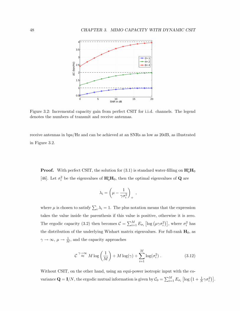
48 CHAPTER 3. MIMO CAPACITY WITH DYNAMIC CSIT
0 5 10 15 200.5
1
1.5
2
2.5
3
3.5
4
SNR in dB
∆C (
bps/
Hz)
2× 14× 28× 4
Figure 3.2: Incremental capacity gain from perfect CSIT for i.i.d. channels. The legenddenotes the numbers of transmit and receive antennas.
receive antennas in bps/Hz and can be achieved at an SNRs as low as 20dB, as illustrated
in Figure 3.2.
Proof. With perfect CSIT, the solution for (3.1) is standard water-filling on H∗0H0
[46]. Let σ2i be the eigenvalues of H∗
0H0, then the optimal eigenvalues of Q are
λi =
(
µ − 1
γσ2i
)
+
,
where µ is chosen to satisfy∑
i λi = 1. The plus notation means that the expression
takes the value inside the parenthesis if this value is positive, otherwise it is zero.
The ergodic capacity (3.2) then becomes C =∑M
i=1 Eσi
[
log(
µγσ2i
)]
, where σ2i has
the distribution of the underlying Wishart matrix eigenvalues. For full-rank H0, as
γ → ∞, µ → 1M , and the capacity approaches
C γ→∞≈ M log
(
1
M
)
+ M log(γ) +M∑
i=1
log(σ2i ) . (3.12)
Without CSIT, on the other hand, using an equi-power isotropic input with the co-
variance Q = I/N , the ergodic mutual information is given by C0 =∑M
i=1 Eσi
[
log(
1 + 1N γσ2
i
)]
.

3.2. ASYMPTOTIC-SNR CAPACITY GAINS 49
At high SNRs, this expression approaches
C0γ→∞≈ M log
(
1
N
)
+ M log(γ) +
M∑
i=1
log(σ2i ) . (3.13)
Subtracting (3.12) and (3.13) side-by-side yields the capacity gain in (3.11). ¤
Rank-deficient channels with non-full-rank Rt
This section considers transmit covariance CSIT with rank-deficient Rt, given zero chan-
nel mean and uncorrelated receive antennas. With rank-deficient Rt, transmit covariance
CSIT helps to increase the capacity additively at high SNRs, regardless of the number of
receive antennas. Let Kt be the rank of Rt (Kt < N), this high-SNR capacity gain can
be precisely quantified in the case Kt ≤ M as
∆C = Kt log
(
N
Kt
)
. (3.14)
The derivation of this result is as follows. For transmit covariance CSIT, the optimal
input beam directions are given by Rt eigenvectors (3.6). Let Λt be the eigenvalue matrix
of Rt, the average mutual information can then be written as
I = EHw[log det (IM + γHwΛtΛQH∗
w)]
= EHw
[
log det
(
IM + γ
Kt∑
i=1
λt,iλQ,ihw,ih∗w,i
)]
= EHw
[
log det(
IKt+ γH∗
w[Kt]Hw[Kt]Λt[Kt]ΛQ[Kt]
)]
,
where Λt[Kt] is the square, diagonal matrix of the non-zero eigenvalues of Λt, ΛQ[Kt] is
the square, diagonal matrix containing the corresponding eigenvalues of Q, and Hw[Kt]
of size M × Kt contains the corresponding Kt columns of Hw. With Kt ≤ M , the
matrix H∗w[Kt]
Hw[Kt]Λt[Kt] has rank Kt, hence at high SNRs, the optimal ΛQ approaches
equi-power on the Kt non-zero eigen-modes of Λt. (This equi-power input is not always
optimal at high SNRs if Kt > M , but a capacity gain still exists.) Without the CSIT,
however, the optimal input distributes power equally on all N eigen-modes of Rt. The

50 CHAPTER 3. MIMO CAPACITY WITH DYNAMIC CSIT
1 2 3 4 5 6 7 82
3
4
5
6
7
8
9
10
11
12
Number of receive antennas M
Erg
odic
cap
acity
(bi
ts/s
ec/H
z)
Rt known, N = 2M
Rt known, N = M
Rt unknown
Rt unknown + gain
Figure 3.3: Capacity of channels with rank-one transmit correlation at SNR = 10dB,without and with transmit covariance CSIT.
difference in the corresponding mutual information then results in (3.14), similar to the
proof of Theorem 4.
Figure 3.3 provides an example of the capacity with and without transmit covariance
CSIT for rank-one correlated channels with various antenna configurations at 10dB SNR.
The capacity without CSIT plus the gain (3.14) is also included. For rank-one correlation,
having more transmit antennas helps to increase the capacity with transmit covariance
CSIT, but does not without the CSIT.
3.3 Optimal input characterizations
The capacity-optimal input signal with dynamic CSIT can be analytically established
in certain cases. At low SNRs, as specified in Theorem 1, it is typically single-mode
beamforming with the direction as a function of CSIT. Hence, mode-dropping almost
always occurs at low SNRs. At high SNRs, the optimal input depends not only on the
CSIT, but also on the antenna configurations. For systems with equal or fewer transmit
than receive antennas, the optimal input approaches isotropic equi-power. For systems
with more transmit than receive antennas, however, it may not approach equi-power at
high SNRs, depending on the CSIT. Specifically, for statistical CSIT with high-K mean

3.3. OPTIMAL INPUT CHARACTERIZATIONS 51
or highly-conditioned transmit covariance, signifying strong antenna correlation, mode-
dropping may also occur at high SNRs. The intuition can be obtained by considering
a 4 × 2 channel with different CSIT. With perfect CSIT, the optimal input has only 2
eigen-modes at high SNRs. Without CSIT, however, the optimal input at all SNRs is
i.i.d. isotropic, which has 4 modes. Therefore there exists partial CSIT, with which the
optimal input has 3 modes at high SNRs, implying mode-dropping.
This section considers impacts of antenna configurations and the CSIT on the optimal
input covariance. It first briefly discusses the optimal input for systems with N ≤ M . It
then provides simplified analysis on the conditions for mode-dropping at high SNRs in
systems with N > M . Two effects are considered: of the K factor and of the transmit
antenna correlation. To isolate each effect, a simplified channel model is used in each
case.
3.3.1 Systems with equal or fewer transmit than receive antennas
For N ≤ M systems with dynamic CSIT, the optimal input signal is known asymptoti-
cally at both low and high SNRs. At low SNRs, it is typically single-mode beamforming
(Theorem 1), and at high SNRs, it approaches equi-power. Interestingly, the optimal
input covariance here can be closely approximated by the closed-form Jensen input co-
variance, discussed in Section 3.5.1. This Jensen covariance becomes optimal at both low
and high SNRs. At other SNRs, it produces a mutual information that is a tight lower-
bound to the capacity. For the two special cases, transmit covariance CSIT and mean
CSIT, the Jensen beam directions are optimal at all SNRs; only the power allocation is
then approximated. More details can be found in Section 3.5.1.
3.3.2 Systems with more transmit than receive antennas
For N > M systems with dynamic CSIT, the capacity-optimal input, especially its power
allocation, depends heavily on the channel effective mean and covariance matrices. If the
channel is uncorrelated with zero mean, as with i.i.d. Rayleigh fading, then the optimal
input covariance is the identity matrix at all SNRs [6], implying equi-power allocation.
However, if the mean is strong, characterized by a high K factor, or the transmit antennas

52 CHAPTER 3. MIMO CAPACITY WITH DYNAMIC CSIT
are highly correlated, characterized by a large condition number of Rt, the optimal input
may drop modes not only at low SNRs (Theorem 1) but also at high SNRs. A closed-
form solution for the optimal input covariance, as a function of the channel mean and
covariance, is still unknown. Furthermore, at high SNRs, the Jensen covariance, which
approaches equi-power, is no longer a good approximation.
This section provides some simple characterizations on effects of the K factor and the
transmit antenna correlation on the optimal input at high SNRs. The analysis focuses
on two simple channel models, belonging to the special mean CSIT and covariance CSIT
cases. Of these, the optimal beam directions are known (3.4), (3.6), thus only the power
allocation needs to be specified. Each considered model results in the optimal allocation
with only two distinct power levels. Conditions that lead to dropping the lower power
level at high SNRs are analyzed.
Effects of the K factor
In an uncorrelated channel with N > M , given statistical CSIT, as K increases from 0 to
infinity, the optimal number of input modes at high SNRs reduces from N to M . Thus,
a sufficiently high K will result in less than N optimal modes, leading to mode-dropping
at high SNRs. The mode-dropping effect, however, depends more broadly on the channel
mean eigenvalues, of which K is a function. To isolate the impact of K alone, consider
an uncorrelated channel, in which the channel mean has equal eigenvalues and hence is
unitary. Thus, the power allocation here depends solely on K, but not the entire Hm.
The threshold for K, above which mode dropping occurs at high SNRs, can be obtained
as stated in the following theorem.
Theorem 5. Consider a channel (2.28) with N > M , uncorrelated antennas, and unitary
channel mean. Specifically, the mean and transmit covariance are given as
HmH∗m =
K
K + 1IM (3.15)
Rt =1
K + 1IN ,
and the receive covariance is Rr = I. With statistical CSIT, the condition on K, with

3.3. OPTIMAL INPUT CHARACTERIZATIONS 53
which the optimal input activates only M out of the maximum N modes at all SNRs, is
given as
tr
Ehw,j
M∑
j=1
(√Kej + hw,j
) (√Kej + hw,j
)∗
−1
≤ 1 , (3.16)
where ei is the M -vector with the ith element equal to 1 and the rest zero, and hw,j ∼N (0, IM ) are i.i.d.
The matrix expression under expectation in (3.16) has the inverted non-central com-
plex Wishart distribution. This expectation has no closed-form solution so far, but can
be evaluated numerically.
Proof: Given mean and transmit covariance (3.15), let β =√
K/(K + 1), and
perform the SVD of the mean as
Hm = βUmV∗m , (3.17)
then the optimal beam directions are given by Vm (3.4). The optimal power alloca-
tion can be completely characterized by the K factor, or β, and the SNRs. Because
of symmetry, this optimal solution contains only two different power levels: λ1 for
the first M eigen-modes, corresponding to the non-zero eigen-modes of H∗mHm, and
λ2 for the rest N −M modes, where λ1 ≥ λ2 [51]. Thus the optimal solution Q for
problem (3.1) has the form
Q = VmΛQV∗m , (3.18)
where ΛQ is a diagonal matrix with M diagonal entries as λ1 and N − M as λ2.
Let H be the zero-mean part of U∗mHVm, then its N columns are i.i.d. with the
distribution hj ∼ N(
0, (1 − β2)IM
)
. The first M columns of U∗mHVm can then

54 CHAPTER 3. MIMO CAPACITY WITH DYNAMIC CSIT
be expressed as βei + hi, 1 ≤ i ≤ M . Problem (3.1) can now be written as
maxλ1,λ2
Ehi
[
log det
(
IM + λ1γM∑
i=1
(
βei + hi
) (
βei + hi
)∗
+ λ2γN
∑
i=M+1
hih∗i
)]
subject to Mλ1 + (N − M)λ2 = 1 (3.19)
λ1 ≥ 0, λ2 ≥ 0 .
Of interested is the condition on K (or β) that results in the optimal λ?1 = 1/M , and
hence λ?2 = 0, implying mode-dropping. Based on the convexity of this problem,
the sufficient and necessary condition for this optimality is
tr
Ehj
I +γ
M
M∑
j=1
(βej + hj)(βej + hj)∗
−1
≤ M
1 + γ (1 − β2), (3.20)
where hj ∼ N(
0, (1 − β2)IM
)
. The derivation is given in Appendix A.1. This
condition depends on M , β and γ and can be evaluated numerically. The condition,
however, is independent of the number of transmit antennas N . From this condition,
a threshold for K, above which mode-dropping occurs, can be established. As
γ → ∞, it becomes (3.16), which signifies mode-dropping at all SNRs. ¤
The threshold (3.20) is independent of the number of transmit antennas N . Thus
if the channel mean is strong enough, the rank of this mean will dictate the number of
active modes, regardless of the larger number of antennas. Figure 3.4 provides examples
of this K factor threshold versus the SNR, derived from (3.20), for systems with 2 receive-
and more than 2 transmit-antennas. When K is above this threshold, signifying a strong
channel mean or a good channel estimate, the optimal power allocation activates only
two modes and drops the rest at all SNRs.
Effects of the transmit antenna correlation
In a zero-mean channel, the condition number of the transmit covariance matrix Rt
can influence the number of optimal input modes. When the condition number is 1,
corresponding to an identity covariance matrix, all N transmit modes are active. When

3.3. OPTIMAL INPUT CHARACTERIZATIONS 55
0 5 10 15 20 25 300
1
2
3
4
5
6
7
SNR (dB)
K th
resh
old
(dB
)
Figure 3.4: K factor thresholds for systems with 2 receive and more than 2 transmitantennas, above which using 2 modes is capacity-optimal for the mean CSIT (3.15) at allSNRs.
the condition number is infinite, implying a rank-deficient covariance Rt, the number
of active modes must be less than N at all SNRs, as no power should be allocated in
Rt null-space. Thus there must be a finite threshold for Rt condition number, above
which mode-dropping occurs at all SNRs. Similar to the K factor, however, Rt condition
number is a function of the eigenvalues, on which the optimal input power allocation
depends. To isolate the impact of Rt condition number, consider a zero-mean channel
with a transmit covariance matrix having only two distinct eigenvalues. The threshold on
the condition number of this matrix for mode-dropping at all SNRs is given as follows.
Theorem 6. Consider a zero-mean channel (Hm = 0) with correlated transmit antennas
and uncorrelated receive antennas. Furthermore, the transmit covariance matrix has the
eigen-value decomposition as
Rt = Ut diag (ξ1 . . . ξ1 ξ2 . . . ξ2) U∗t , (3.21)
in which L eigenvalues equal ξ1 and N − L equal ξ2, provided N > L > M and ξ1 > ξ2.
With statistical CSIT, the threshold for Rt condition number, κ = ξ1/ξ2, above which

56 CHAPTER 3. MIMO CAPACITY WITH DYNAMIC CSIT
mode-dropping occurs at all SNRs, is given as
κ ≥ L
L − M. (3.22)
This condition requires N ≥ M + 2.
Proof: Given zero channel mean and transmit covariance (3.21), the optimal input
covariance Q has the eigenvectors given by Ut (3.6). Again because of symmetry,
the optimal power allocation has only two levels: λ1 for the first L eigen-modes
corresponding to the L larger eigenvalues of Rt, and λ2 for the rest N − L modes.
The optimal Q therefore has the EVD as
Q = UtΛQU∗t , (3.23)
where ΛQ is a diagonal matrix with L diagonal entries as λ1 and N − L as λ2.
From (2.18), the channel can be written as H = HwR1/2t . Let H = HwUt, then
the N columns of H are i.i.d. with distribution hi ∼ N (0, IM ), 1 ≤ i ≤ N . The
mutual information optimization problem (3.1) is now equivalent to
maxλ1,λ2
Ehi
log det
IM + γλ1ξ1
L∑
j=1
hih∗i + γλ2ξ2
N∑
j=L+1
hih∗i
(3.24)
subject to Lλ1 + (N − L)λ2 = 1
λ1 ≥ 0 , λ2 ≥ 0 .
Of interest is the condition that results in the optimal λ?2 = 0 and λ?
1 = 1/L.
Based on the convexity of this problem, the sufficient and necessary condition for
the optimal λ2 = 0 is
tr
Ehi
IM +γξ1
L
L∑
j=1
hih∗i
−1
(γξ2 + 1)
≤ M , (3.25)
where hj ∼ N (0, IM ). The derivation is given in Appendix A.2. At high SNRs

3.3. OPTIMAL INPUT CHARACTERIZATIONS 57
(γ → ∞), this condition becomes
Lξ2
ξ1tr
Ehi
L∑
j=1
hih∗i
−1
≤ M .
Noting that the matrix under expectation is an inverted complex central Wishart
matrix with rank M and L degrees of freedom, which has the first moment as
IM/(L − M) [59, 47], the above condition results in (3.22). The finite expectation
requires L > M , and since N > L, this relation implies N ≥ M + 2. Thus, mode
dropping at all SNRs occurs only if N ≥ M +2. Consequently, as the SNR increases
to infinity, the optimal power allocation for this transmit covariance CSIT always
activate at least M + 1 modes. ¤
From (3.22), noting that L/(L−M) ≤ N −1, a looser bound on Rt condition number
for dropping the weaker eigen-modes at all SNRs can be obtained as
κ =ξ1
ξ2≥ N − 1 . (3.26)
This condition can be used as the first check for mode-dropping.
Figure 3.5 shows an example of the optimal power allocation for a 4 × 2 zero-mean
channel with transmit covariance eigenvalues as [1.25 1.25 1.25 0.25]. This covariance
matrix has the condition number κ = 5 > 3, satisfying (3.22). The optimal power
allocation therefore only activates 3 modes, dropping 1 mode, at all SNRs.
Remarks
The two conditions (3.16) and (3.22), although specific to each respective channel and
CSIT model, provide intuition on effects of the channel mean and the transmit antenna
correlation on the optimal input power allocation. The conditions for channels with both
non-zero mean and transmit antenna correlation are likely to be further relaxed, such
that mode dropping occurs at all SNRs for even a lower K factor and a lower correlation
condition number. Subsequently, for N > M , channels with high K or strong transmit
antenna correlation tend to result in mode dropping with statistical CSIT at all SNRs.

58 CHAPTER 3. MIMO CAPACITY WITH DYNAMIC CSIT
−10 0 10 20 30 400
0.05
0.1
0.15
0.2
0.25
0.3
0.35
0.4
SNR in dB
Tra
nsm
it co
varia
nce
eige
nval
ues
Optimal powerJensen powerEqual power
Figure 3.5: Input power allocations for a 4×2 zero-mean channel with transmit covarianceeigenvalues [1.25 1.25 1.25 0.25]. Each allocation scheme contains 4 power levels,corresponding to the 4 eigen-modes of the transmit covariance. The optimal allocationhas 3 equal modes, as does the Jensen power at low SNRs. The fourth mode of theoptimal scheme always has zero power.
3.4 Capacity optimization
The previous sections have analytically established asymptotic capacity gains and the
optimal input covariance at low and high SNRs. This section focuses on building an
optimization program to solve for the capacity (3.1) non-asymptotically at any SNR. The
program assumes channel model (2.28), in which the channel has a non-zero mean and
correlated transmit antennas, but uncorrelated receive. The transmitter has statistical
CSIT consisting of the mean and the transmit covariance.
Problem (3.1) is convex, hence solving for Q can be performed numerically up to a
desired precision. Since Q is a Hermitian matrix of size N ×N , it contains N2 real scalar
variables. These include N real entries on the diagonal and 12N(N −1) complex entries in
the upper triangle, each contributes two real variables. Thus, the optimization variable
size is N2.
For the special CSIT cases, in which the eigenvectors UQ of the optimal Q are known
analytically (3.4, 3.6), the optimization only needs to find the eigenvalues ΛQ. Let
S = γU∗QH∗HUQ , (3.27)

3.4. CAPACITY OPTIMIZATION 59
then S is known perfectly at the receiver and its distribution is known at the transmitter.
Using det(I + AB) = det(I + BA), problem (3.1) now becomes
max ES[log det(I + SΛQ)] (3.28)
subject totr(ΛQ) = 1
ΛQ < 0 ,
where ΛQ is a diagonal matrix of size N ×N , and the expectation is performed over the
known distribution of S. The number of unknowns here is reduced to N real variables.
3.4.1 Convex optimization methods
The Newton method is used to solve both problems (3.1) and (3.28). In problem (3.1),
when the positive semidefinite constraint Q < 0 is active, meaning some eigenvalues
of the optimal Q are zero, the program employs a barrier interior-point method, using
the Newton method for the inner iterations [54]. Such a barrier implementation is not
necessary for problem (3.28) because of the simple diagonal structure of ΛQ. In both
problems, since the expectation in the objective function has no closed-form, the under-
lying stochastic nature complicates the optimization by making it difficult to compute
the exact function value, the gradient, and the Hessian needed at each optimization step.
These values are approximated using sets of channel samples. As the number of transmit
antennas N grows, the number of samples needs to be increased. The gap between the
current function value and the optimal value, or the function gap-to-optimal value used
in the stopping criterion, is also approximated by Monte-Carlo simulations. Therefore,
the variance of these sample means dictates the numerical precision.
Solving for the eigenvalues ΛQ in the special CSIT cases
Consider first the simpler problem (3.28) with N real variables. Denote λ = diag(ΛQ),
a real column-vector consisting of the N unknown eigenvalues. The problem becomes an
optimization in λ with the equality constraint 1T λ = 1 and inequality λ < 0 (element-
wise). The Newton method can be implemented very efficiently. The condition λ < 0 is
handled as follows: when ever a Newton step produces a negative λi value, this eigenvalue

60 CHAPTER 3. MIMO CAPACITY WITH DYNAMIC CSIT
is set to zero, and the optimization continues with the other variables, re-adjusted for the
unit sum. This step is equivalent to dropping a mode in a water-filling process.
The Newton method requires calculating the gradient and the Hessian of the objective
function. Noting that the objective function in (3.28) has no closed-form, the expectation
operator is approximated by taking the sample mean over a set of channel samples.
An independent set of samples is generated for each Newton step to ensure that the
approximation, and therefore the optimization result, is independent of any particular
sample set. For each channel sample, compute the following matrices
P = I + SΛ , Y = P−1 , Z = YS . (3.29)
The largest computational cost is calculating Y, due to the matrix inversion. The gradient
of the log det function in (3.28) with respect to λ is then a N ×1 row-vector with elements
given by [60]
(∇g)i = −E
[
tr
(
P−1 ∂P
∂λi
)]
= −E[
yTi si
]
= −E [Zii] , i = 1 . . . N
where yTi is row i of Y, si is column i of S, and Zii is the ith diagonal element of Z. The
Hessian can also be formed as a N × N matrix with elements given by
(
∇2g)
ij= E
[
tr
(
P−1 ∂P
∂λiP−1 ∂P
∂λj
)]
= E[
yTj siy
Ti sj
]
= E [ZjiZij ] , (3.30)
i, j = 1 . . . N .
The gradient and the Hessian of the objective function are then obtained as the mean of
these values over all channel samples.
For these special CSIT cases, transmit power optimization (3.28) can also be effi-
ciently performed using an iterative algorithm involving the MMSE of the data streams
transmitted on separate eigen-beams [61]. This algorithm requires predetermined beam
directions and finds the optimal power allocation along those beams. For general statis-
tical CSIT, however, the optimal beam directions are still unknown. The next section
describes a method for solving for the optimal Q? in that case.

3.4. CAPACITY OPTIMIZATION 61
Solving for the covariance Q in the general case
The general problem (3.1) is similarly solved using the Newton method. Because of the
matrix form of the unknown Q, however, the PSD constraint Q < 0 needs special han-
dling. Specifically, a barrier interior-point method is implemented if this constraint is
active, meaning the optimal Q has at least one zero-eigenvalue. This condition is heuris-
tically established when the initial Newton step without involving the PSD constraint
produces a non-positive semidefinite Q. Otherwise, the program proceeds, ignoring the
PSD constraint. By using a good starting point (such as the Jensen covariance in Section
3.5.1), this heuristic check leads to the optimal solution, while reducing the run time.
For the Newton method, the objective function value and its gradient and Hessian
are again approximated by sample means, using an independent set of channel samples
at each step. The gradient and the Hessian in each Newton step are computed as follows.
Since Q is a Hermitian matrix, form a vector of unknown variables from the real and
imaginary parts of Q as
q =[q11
2. . .
qNN
2qR21 qR32 . . . qRN1 qI21 qI32 . . . qIN1
]T, (3.31)
where QR = Re(Q), QI = Im(Q), and the lower-case letters refer to the entries in the
corresponding upper-case matrix with the same subscript. The factor 12 is introduced for
uniformity in the gradient and the Hessian formula (with respect to q). The length of q
is N2. For each channel sample, compute G = γH∗H and
R = I + GQ , W = R−1 , X = WG . (3.32)
The most intensive step is to compute W, involving matrix inversion. Once X is com-
puted, the gradient and the Hessian follow directly. Noting that X is Hermitian, the
gradient of the log det function in (3.1) has the elements given as
∂f
∂qRij= −E
[
tr
(
R−1 ∂R
∂qRij
)]
= −E[
wTj gi + wT
i gj
]
= −2E [Re(X)ij ] (3.33)
∂f
∂qIij= −E
[
tr
(
R−1 ∂R
∂qIij
)]
= −jE[
wTj gi − wT
i gj
]
= −2E [Im(X)ij ] ,

62 CHAPTER 3. MIMO CAPACITY WITH DYNAMIC CSIT
where wTi is row i of W, gi is column i of G, and Re(.) and Im(.) represent the real and
imaginary parts. The Hessian has the elements calculated as
∂2f
∂qRij∂qRkl= 2E [Re(XljXik + XkjXil)]
∂2f
∂qIij∂qIkl= 2E [Re(XljXik − XkjXil)] (3.34)
∂2f
∂qRij∂qIkl= 2E [Im(XljXik + XkjXil)]
∂2f
∂qIij∂qRkl= 2E [Im(−XljXik + XkjXil)] .
The gradient and Hessian of the objective function are then obtained as the sample means
of these values over all channel samples.
When the PSD constraint on Q is tight, equivalently the optimal input signal drops
modes, the program uses the barrier method [54], which iteratively solves the following
problem for different values of t:
max EG[log det(I + GQ)] + log det(Q)/t (3.35)
subject to tr(Q) = 1 ,
where G = γH∗H and t > 0. The second term in the objective function, log det(Q)/t,
ensures that Q stays PSD, by choosing a large enough initial value for t. Then during
the optimization, if any eigenvalue of Q approaches zero, log det(Q)/t approaches minus
infinity, preventing this eigenvalue from becoming negative.
Solving (3.35) involves two iterative loops. The inner loop uses the Newton method to
find Q?, given a value of t. The additional term log det(Q)/t is independent of the channel,
thus its gradient and Hessian, established similarly to (3.33) and (3.34) respectively, can
be calculated exactly with little overhead. Then the outer loop increases the barrier value
t by multiplying it with µ, a positive optimization parameter. This increase in t leads to
diminishing impact of log det(Q)/t on the optimal function value. The inner optimization
is performed again for the new value of t, using the previous optimal Q? as the starting
point. Since this starting point is PSD and close to optimal, the new Q? is also PSD,

3.4. CAPACITY OPTIMIZATION 63
1 2 3 4 5 6 7 8 9 100
10
20
30
40
50
60
70
80
90
100
Number of channel samples (× 104)
Ave
rage
run
tim
e pe
r ite
ratio
n (s
ec)
Special casesGen. no barrier
(a)
2 3 4 5 6 7 8 9 100
5
10
15
20
25
30
Number of antennas N = M
Ave
rage
run
tim
e pe
r ite
ratio
n (s
ec)
Special casesGen. no barrierN2 fitN3 fit
(b)
Figure 3.6: Optimization runtime complexity versus (a) the number of channel samples(at N = M = 4) and (b) the number of antennas (N = M , at 10000 samples).
ensured by log det(Q)/t. The two steps are repeated until a desired tolerance is satisfied.
Thus, the barrier implementation takes longer to execute because of this double loop.
3.4.2 Optimization complexity and examples
Complexity assessment
The optimization programs were written using Matlab. Figure 3.6 shows the compu-
tational complexity in terms of program runtime per Newton iteration versus both the
number of channel samples and the number of antennas N = M . The runtime scales
linearly with the number of channel samples, but at different rates for each problem (3.1)
and (3.28). For the number of transmit antennas N in the range of interest (N ≤ 10),
the runtime for the special-case problem (3.28) scales as N2, faster than the order of
N3 predicted by theory [54]. For the general-case problem (3.1) without the barrier
implementation, the runtime scales as N3, not N6 as theoretically predicted.
Numerical examples
Figure 3.7 presents an example of the optimization process for the general problem (3.1),
showing the mutual information value and its gap to the optimal value versus the number

64 CHAPTER 3. MIMO CAPACITY WITH DYNAMIC CSIT
0 2 4 6 8 104.54
4.56
4.58
4.6
4.62
4.64
4.66
4.68
Number of iterations
Fun
ctio
n va
lue
(a)
1 2 3 4 5 6 7 8 9 1010
−5
10−4
10−3
10−2
Number of iterations
f(x k)
− f*
(b)
Figure 3.7: An optimization example of finding the ergodic capacity of a 4× 2 channel atSNR = 10dB, using 20000 independently generated channel samples in each iteration. Theoptimization and channel parameters are given in Appendix B.2. (a) Mutual informationvalue (nats/sec/Hz); (b) Its gap-to-optimal.
of Newton iterations. This example does not invoke the barrier method. The optimiza-
tion parameters and channel mean and covariance are given in the Appendix B.2. The
optimization chooses the starting point as the Jensen covariance (see Section 3.5.1), re-
sulting in a fast convergence. The fluctuation in the function value and its gap-to-optimal
value over different iterations is caused by the approximation of expected values as sample
means, using an independent sample set at each iteration. Thus, the function error-floor
in Figure 3.7(b) is dictated by the number of channel samples, but not the number of
iterations as in deterministic optimization.
3.5 Capacity analysis using the optimization program
The developed program provides a way of evaluating the capacity of a MIMO channel with
statistical CSIT (channel mean and transmit covariance) accurately. The optimization
also results in the optimal input covariance Q?, or its eigenvalues Λ? in the special cases.
The program thus provides a handy tool to study the capacity and the effects of various
channel parameters on it.
The numerical optimization, however, costs time and computational resource. Hence,

3.5. CAPACITY ANALYSIS USING THE OPTIMIZATION PROGRAM 65
it is also of interest to find a simple bound to the capacity and an approximation of the op-
timal input covariance, which can provide analytical insight. The numerical optimization
can help assess the tightness of such a bound.
The next section discusses a simple, sub-optimal input-covariance, based on the Jensen
inequality, and the associated lower-bound to the capacity. Then using this bound and
the numerical optimization program, MIMO capacity is analyzed in terms of various
parameters: relative transmit-receive antenna configurations, the CSIT quality ρ, and
the channel K factor.
3.5.1 Channel capacity and the Jensen-optimal input covariance
Consider maximizing Jensen’s upper-bound on the mutual information, and using its
optimizer QJ to approximate the optimal input covariance Q?. A closed-form analytical
solution for QJ is available. The Jensen bound on the average mutual information is
E [log det(I + HQH∗)] ≤ log det (I + E[H∗H]Q) .
Since with statistical CSIT, the transmitter knows the channel distribution, it can estab-
lish E[H∗H]. Perform the eigenvalue decomposition
E[H∗H] = URDRUR∗ , (3.36)
then the covariance QJ that maximizes the Jensen bound has the eigenvectors given by
UR, and the eigenvalues obtained by standard water-filling on DR as
λi(Q?J) =
(
µ − 1
γdR,i
)
+
, i = 1 . . . N , (3.37)
where dR,i are the diagonal elements of DR, and µ is chosen to satisfy∑N
i=1 λi(QJ) = 1.
That is
QJ = URΛJU∗R , (3.38)
with ΛJ = diag(λi) as given in (3.37).
Using the Jensen covariance QJ as the input covariance results in a Jensen mutual

66 CHAPTER 3. MIMO CAPACITY WITH DYNAMIC CSIT
information value
IJ = I(QJ) (3.39)
satisfying IJ ≤ Io in (3.1). For statistical CSIT, IJ can be used to lower-bound the capac-
ity. For dynamic CSIT, averaging IJ over the initial channel measurement distribution
as in (3.2), a lower-bound to the channel ergodic capacity is obtained as
CJ = EH0[IJ ] . (3.40)
The tightness of this capacity lower-bound depends on the tightness of the Jensen mutual
information in (3.39).
Tightness of the capacity lower-bound based on the Jensen covariance
Using statistical CSIT as a representative, this section discusses the tightness of the Jensen
mutual information (3.39) as a lower-bound to the capacity. The tightness depends on
the relative transmit-receive antenna configuration and the SNR. For systems with equal
or fewer transmit than receive antennas (N ≤ M), results show that the Jensen mutual
information is a tight lower-bound to the capacity at all SNRs. Any minor difference
between IJ and Io occurs only at mid-range SNRs, because of a small difference in power
allocation. Otherwise, at low SNRs, the optimal power allocation is typically single mode,
while at high SNRs, it approaches equi-power, as does the Jensen covariance. Figure 3.8
shows an example of the channel capacity and the Jensen mutual information for a 4× 4
system in (a), together with the eigenvalues of Q? and QJ in (b). The channel has a
non-zero mean and transmit antenna correlation, given in Appendix B.2. The mutual
information with equal power allocation is also included for comparison.
For systems with more transmit than receive antenna (N > M), the Jensen mutual
information is also a tight lower-bound to the capacity at low SNRs. At high SNRs,
however, it exhibits a gap to the capacity. This gap occurs depending on the channel
mean and the transmit antenna correlation. A higher K or more correlated channel
(measured by, for example, a higher condition number of the correlation matrix) will
result in a bigger gap. The main reason for this gap at high SNRs is the difference in the

3.5. CAPACITY ANALYSIS USING THE OPTIMIZATION PROGRAM 67
−5 0 5 10 15 20 25 30
5
10
15
20
25
30
SNR in dB
Mut
ual i
nfor
mat
ion
(bps
/Hz)
Ergodic capacityMI w/Jensen covMI w/equal power
(a)
−5 0 5 10 15 20 25 300
0.1
0.2
0.3
0.4
0.5
0.6
0.7
0.8
0.9
1
SNR in dB
Tra
nsm
it co
varia
nce
eige
nval
ues
Optimum powerJensen powerEqual power
(b)
−5 0 5 10 15 20 25 300
2
4
6
8
10
12
14
16
18
20
SNR in dB
Mut
ual i
nfor
mat
ion
(bps
/Hz)
Ergodic capacityMI w/Jensen covMI w/equal power
(c)
−5 0 5 10 15 20 25 300
0.1
0.2
0.3
0.4
0.5
0.6
0.7
0.8
0.9
1
SNR in dB
Tra
nsm
it co
varia
nce
eige
nval
ues
Optimum powerJensen powerEqual power
(d)
Figure 3.8: Capacity and mutual information of (a) a 4 × 4 system, (c) a 4 × 2 system;with the corresponding power allocations in (b) and (d). The channel mean and transmitcovariance are specified in Appendix B.2.
power allocation. In contrast to equi-power in the Jensen solution, the capacity-optimal
input can converge to non-equi-power. The optimal convergence values are still unknown
analytically. Using simplified channel models, section 3.3 examines conditions for the
optimal input to have at least one zero-power mode at high SNRs. Figures 3.8(c) and
(d) illustrate the mutual information and the input power allocations for a 4× 2 channel
with the mean and correlation matrices given in Appendix B.2.
These comparisons also reveal that the value of CSIT depends on the antenna config-
uration and the SNR. For N ≤ M , CSIT helps increase the capacity only at low SNRs.
At high SNRs, the optimal input approaches equi-power and the capacity gain from CSIT

68 CHAPTER 3. MIMO CAPACITY WITH DYNAMIC CSIT
0 0.2 0.4 0.6 0.8 14.8
5
5.2
5.4
5.6
5.8
6
6.2
6.4
6.6
6.8
Estimate quality ρ
Erg
odic
cap
acity
(bi
ts/s
ec/H
z)
CH1: 4 × 4 i.i.d.CH2: correlated RayleighCH2 without Tx−CSI
(a) 4 × 4 channels.
0 0.2 0.4 0.6 0.8 12.8
3
3.2
3.4
3.6
3.8
4
4.2
4.4
4.6
4.8
Estimate quality ρ
Erg
odic
cap
acity
(bi
ts/s
ec/H
z)
CH1: 4 × 2 i.i.d.CH2: correlated RicianCH2 without Tx−CSI
(b) 4 × 2 channels.
Figure 3.9: Ergodic capacity versus the CSIT quality ρ at SNR = 4dB.
diminishes. For N > M , however, CSIT can help increase the capacity at all SNRs. The
asymptotic capacity gains at low and high SNRs are quantified in Section 3.2.
3.5.2 The capacity versus dynamic CSIT quality
Since the Jensen mutual information is a tight lower-bound to the capacity at low SNRs,
it is used to plot the capacity versus the CSIT quality ρ in Figure 3.9. The capacity
increases with higher ρ. The increment, however, is sensitive to ρ only when ρ is larger
than about 0.6, corresponding to a relatively good channel estimate. This observation
implies that in dynamic CSIT, the initial channel measurement adds value only when its
correlation with the current channel is relatively strong; otherwise, the channel statistics
provide most information.
Two antenna configurations are examined in Figure 3.9: 4×4 in (a) and 4×2 in (b). In
each configuration, an i.i.d. Rayleigh fading channel and a correlated Rician channel are
studied. The mean and covariance matrices of the correlated Rician channels are given
in Appendix B.2. Results show that the range of capacity gain from the CSIT for the
i.i.d. channels is larger than for the correlated ones. Note that as the SNR increases, the
capacity gains for the 4×4 channels decrease to 0, but increase for the 4×2 channels to up
to 2 bps/Hz (3.11). For reference, the capacity of the correlated Rician channels without
CSIT is also included. For correlated Rician channels, knowing the channel statistics

3.5. CAPACITY ANALYSIS USING THE OPTIMIZATION PROGRAM 69
−20 −10 0 10 20 30 40
1.4
1.6
1.8
2
2.2
2.4
2.6
K factor in dB
Mut
ual i
nfor
mat
ion
(bps
/Hz)
CapacityJensen MIEqual power
(a) SNR = -2dB.
−20 −10 0 10 20 30 406.5
7
7.5
8
8.5
9
9.5
10
K factor in dB
Mut
ual i
nfor
mat
ion
(bps
/Hz)
CapacityJensen MIEqual power
(b) SNR = 12dB.
Figure 3.10: Ergodic capacity and mutual information versus the K factor.
alone (ρ = 0) can enhance the capacity. Furthermore, at low SNRs, correlated Rician
channels can have higher capacity than i.i.d. Rayleigh ones, as shown in (b).
3.5.3 Effects of the K factor
The channel Rician K factor affects the ergodic capacity differently depending on the
SNR. Figure 3.10 shows the capacity versus K at two different SNRs for 4 × 2 channels
with the mean and covariance given in Appendix B.2. Notice that at a low SNR (-2dB),
the capacity is a non-monotonous function of the K factor, and a minimum exists. This
effect is partly caused by the transmit antenna correlation impact: at low K, the correla-
tion effect becomes more dominant, and at low SNRs, this correlation helps increase the
capacity. At a higher SNR (12 dB), the correlation impact diminishes for full-rank corre-
lation. Provided that the channel mean is also full-rank, the capacity then monotonically
increases with the K factor. The increment, however, diminishes with higher K.
For systems with more transmit than receive antennas, a higher K factor also causes
the SNR point, at which the Jensen mutual information starts diverging from the channel
capacity, to increase. This effect implies that with higher K factor, the Jensen mutual
information is a tight lower-bound to the capacity for a larger range of SNRs. Figure
3.11 presents this K factor threshold versus the SNR for the 4 × 2 channels. When K is
above this threshold, the Jensen mutual information tightly lower-bounds the capacity.
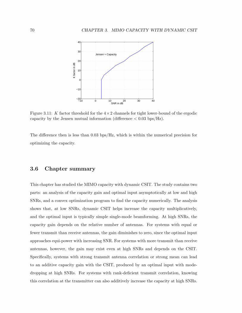
70 CHAPTER 3. MIMO CAPACITY WITH DYNAMIC CSIT
−10 0 10 20 30 40−20
−10
0
10
20
30
40
K fa
ctor
in d
B
SNR in dB
Jensen ≈ Capacity
Figure 3.11: K factor threshold for the 4×2 channels for tight lower-bound of the ergodiccapacity by the Jensen mutual information (difference < 0.03 bps/Hz).
The difference then is less than 0.03 bps/Hz, which is within the numerical precision for
optimizing the capacity.
3.6 Chapter summary
This chapter has studied the MIMO capacity with dynamic CSIT. The study contains two
parts: an analysis of the capacity gain and optimal input asymptotically at low and high
SNRs, and a convex optimization program to find the capacity numerically. The analysis
shows that, at low SNRs, dynamic CSIT helps increase the capacity multiplicatively,
and the optimal input is typically simple single-mode beamforming. At high SNRs, the
capacity gain depends on the relative number of antennas. For systems with equal or
fewer transmit than receive antennas, the gain diminishes to zero, since the optimal input
approaches equi-power with increasing SNR. For systems with more transmit than receive
antennas, however, the gain may exist even at high SNRs and depends on the CSIT.
Specifically, systems with strong transmit antenna correlation or strong mean can lead
to an additive capacity gain with the CSIT, produced by an optimal input with mode-
dropping at high SNRs. For systems with rank-deficient transmit correlation, knowing
this correlation at the transmitter can also additively increase the capacity at high SNRs.

3.6. CHAPTER SUMMARY 71
The second part focuses on a convex program to calculate the capacity with statis-
tical CSIT, involving a non-zero mean and transmit antenna correlation. The program
employs the Newton and barrier interior-point methods. Due to the underlying stochas-
tic nature, the gradient, Hessian, and function values in each Newton step are evaluated
using Monte-Carlo simulations. The computational cost grows linearly with the number
of channel samples in Monte-Carlo, and quadratically-to-cubically with the number of
transmit antennas. The program is then used to assess a capacity lower-bound based on
the Jensen-optimal input. This simple lower-bound is often tight at all SNRs for systems
with equal or fewer transmit than receive antennas. For others, the bound is tight at
low SNRs but diverges at high SNRs. This divergence at high SNRs is caused by the
difference in power allocation and depends on the CSIT – the channel mean and the
transmit antenna correlation. A stronger mean or correlation causes a larger divergence.
Furthermore, a higher channel K factor results in later divergence at a higher SNR.
Applied to dynamic CSIT, optimization results illustrate an increasing capacity with
better CSIT quality ρ. The capacity gain from the CSIT, however, is sensitive to ρ for
large ρ only, at roughly ρ ≥ 0.6. Otherwise, the gain equals that with ρ = 0, corresponding
to statistical CSIT. Furthermore, the capacity gain depends not only on ρ but also on
the channel statistics. Compared to a correlated Rician channel, the gain is higher for an
i.i.d. Rayleigh fading channel at high CSIT quality ρ, but becomes lower as ρ decreases.
Having analyzed the capacity gain from dynamic CSIT, the next chapter will discuss
precoding designs to exploit the CSIT.

Chapter 4
PRECODING SCHEMES
EXPLOITING DYNAMIC CSIT
Precoding is a transmitter processing technique that exploits CSIT. As discussed in Sec-
tion 1.2, the separation between a precoder, dependent on the CSIT, and a channel code,
independent of the CSIT, is capacity-optimal for many CSIT forms, including dynamic
CSIT. For flat-fading MIMO channels, the optimal precoder is linear. It functions as a
multimode beamformer. The beam directions and power allocation are the left singular
vectors and the squared singular values of the precoding matrix, respectively. The right
singular vectors function as an input shaping matrix.
This chapter focuses on designing linear precoders for dynamic CSIT. A precoder
can be designed according to alternative criteria, roughly categorized as fundamental
and practical. An example of a fundamental criterion is the system ergodic capacity. The
precoder then shapes the covariance of the optimal zero-mean Gaussian input. A practical
criterion, on the other hand, can be minimizing an error probability for a specific system.
A common system configuration includes a space-time block code (STBC) exploiting
channel diversity and a linear precoder exploiting the CSIT. STBCs are often designed for
i.i.d. Rayleigh fading channels, assuming no CSIT. The STBC and precoder combination,
therefore, is robust to channel fading and can exploit the available CSIT at the same time.
Moreover, if the STBC is capacity-lossless without CSIT, then the combined configuration
72

73
is capacity-optimal with CSIT. Such a setup also provides flexibility in designing precoders
to adapt to various CSIT conditions, without changing the STBC or the detection scheme
in an existing system.
MIMO precoding design has been an active research area. Many of the earlier designs
focused on the perfect CSIT case, often jointly optimizing both the precoder and decoder
for various performance criteria based on the MSE or the SNR [62, 63, 64]. More recent
work considered partial CSIT, but only the special cases of transmit covariance CSIT
and mean CSIT. These include precoders optimal for the channel ergodic capacity, given
transmit covariance CSIT [48, 49, 55], or mean CSIT [48, 50, 65]. Others are based on
an error rate criterion with mean CSIT [42, 66, 67], or transmit covariance CSIT [68, 69].
The precoding solutions for these partial-CSIT cases then reduce to fixed beam directions
at all SNRs, given by the singular- or eigen-vectors of the mean or transmit covariance
matrix, with per-beam power allocation, obtained by a numerical water-filling solution
dependent on the SNR.
This chapter first considers a precoder that simultaneously exploits both the channel
mean and the transmit covariance to minimize the pair-wise error probability (PEP) in
MIMO systems. Because of the interaction of the mean and the covariance, the precoder
solution does not have predetermined beam directions. Instead, both the direction and
power loading of each beam depend on both the mean and covariance matrices, and are
functions of the SNR. The optimal precoder is established using a dynamic water-filling
process, in which the beams direction and power evolve with each iteration. Asymptotic
analyses reveal that the precoder depends primarily on the channel mean at high K
factors and primarily on the transmit covariance at high SNRs.
The precoder can be directly applied to dynamic CSIT, exploiting the effective mean
and effective transmit covariance. It achieves a coding gain in the form of an SNR
advantage, attributed to the optimal beam directions and the water-filling-type power
allocation among these beams. When the CSIT is partial, no diversity gain can be
extracted from the channel information. The transmit diversity is then controlled by the
STBC. When the CSIT is perfect, the precoder achieves the maximum diversity order,
together with the coding gain.

74 CHAPTER 4. PRECODING SCHEMES EXPLOITING DYNAMIC CSIT
In addition to the PEP-based precoder, this chapter also briefly examines precoders
based on the capacity of a system using a predetermined code, posed as a stochastic op-
timization problems. Only special CSIT cases are considered here. The precoder optimal
input shaping matrix and beam directions are discussed. The chapter then provides a
comparative analysis of these different precoders in terms of structure and performance.
The chapter is organized as follows. Section 4.1 outlines the system configuration.
Section 4.2 discusses the precoding design criteria based on the PEP and the system
capacity. The optimal precoder based on the PEP is discussed in Section 4.3. Section
4.4 analyzes the gain, asymptotic behavior, and special cases of this precoder design.
Other precoding designs based on the system capacity, generalized to stochastic criteria,
for special CSIT cases are discussed in Section 4.5. Section 4.6 compares these precoders
structure and performance. Finally, Section 4.7 provides a summary.
4.1 System configuration
For precoding design, consider a Rician channel with transmit antenna correlation alone.
The channel model is given in (2.18), but with Rr = I. Furthermore, the transmit
covariance matrix Rt is assumed to be full-rank and, hence, is invertible. The rank
of the channel mean Hm, on the other hand, can be arbitrary. Dynamic CSIT for this
channel is obtained accordingly from (2.25) and (2.27). Since dynamic CSIT consists of an
effective channel mean and an effective covariance, a precoding design for dynamic CSIT
can also be applied to any CSIT model with known channel mean and covariance at the
transmitter. Thus, in the sequel, design algorithms are developed for the representative
case of statistical CSIT, consisting of the mean Hm and the transmit covariance Rt. The
algorithms can then be applied to dynamic CSIT by replacing Hm with the effective mean
and Rt with the effective transmit covariance.
Consider a system in which the transmitter contains an encoder and a linear precoder,
depicted in Figure 4.1. The encoder assumes no channel knowledge, and the precoder
exploits the CSIT. The encoder can include either a channel code, a space-time code, or

4.1. SYSTEM CONFIGURATION 75
NW^
i.i.d.Gaussian
CSIT
Transmitter
FPrecoder
EncoderC XW Channel
HY
Decoder
Figure 4.1: Configuration of a system with linear precoder.
both. In such a system, the precoder can be viewed as a processing block to enhance per-
formance in addition to existing codes, based on the available CSIT. This scenario covers
many practical wireless systems, such as those in wireless local-area-networks (802.11) and
metropolitan-area-networks (802.16). Furthermore, if the encoder is capacity-optimal for
a channel without CSIT, then combining it with a linear precoder is optimal with CSIT
[13]. The capacity-optimal signal for an i.i.d. Rayleigh fading MIMO channel without
CSIT is zero-mean complex Gaussian with an identity covariance matrix [6]. Therefore,
the linear precoder has the effect of shaping the transmit signal, such that it has a co-
variance matrix optimal for the channel with CSIT.
At each time instant, the linear precoder functions as a beamformer with either one
or multiple beams, as analyzed in Section 1.3. The beam directions are the left singular
vectors of the precoder matrix; the beam power loadings are the squared singular values.
The precoder right singular vectors form an input shaping matrix, which combines the
output symbols of the encoder to feed into each beam. A separate precoder provides
the flexibility of adapting to various CSIT conditions, without changing the encoder or
the detection algorithm already implemented. Detection in a system with precoding is
performed over the effective channel created by the precoder and the actual channel.
The receiver can construct the precoder using the same algorithm and parameters as
the transmitter, which implicitly implies that the receiver must know all the parameters
that the transmitter knows. This assumption is reasonable since the receiver can usually
obtain channel measurements more readily than the transmitter through the use of pilots,
and both can agree on using the same precoding design algorithm.
To maintain a constant average sum transmit power, the precoding matrix must satisfy

76 CHAPTER 4. PRECODING SCHEMES EXPLOITING DYNAMIC CSIT
the power constraint
tr(FF∗) = 1. (4.1)
Consider a block encoder with C as a codeword of size N × T , the receive signal block,
of size M × T , can be written as
Y = HFC + N ,
where N ∼ N (0, Iσ2) is the additive complex white Gaussian noise, with σ2 being the
noise power per spatial dimension. The codeword C here has been scaled according to
the transmit power.
To focus on exploiting CSIT, the ideal maximum-likelihood (ML) receiver is used.
The decoded codeword therefore is obtained as
C = arg minC∈C
||Y − HFC||2F , (4.2)
where C is the codebook, and the subscript F here denotes the Frobenius norm.
4.2 Precoding design criteria
A linear precoder can be designed based on alternate criteria, using either a fundamental
or practical measure. The fundamental measures include the capacity and the error ex-
ponent, while the practical measures contain, for example, the pair-wise error probability
(PEP), detection mean square-error (MSE), and the received SNR [19]. Fundamental
measures usually assume ideal channel coding. The ergodic capacity assumes that the
channel evolves through all possible realizations over arbitrarily long codewords, while the
error exponent applies for finite codeword lengths. Analyses using practical measures, on
the other hand, usually apply to uncoded systems and assume a quasi-static block-fading
channel. The choice of the design criterion depends on the system setup, operating param-
eters, and the channel (fast or slow fading). For examples, systems with strong channel
coding, such as turbo or low-density parity check codes with long codewords, may operate
at close to the capacity limit and thus are qualified to use a coded fundamental criterion.

4.2. PRECODING DESIGN CRITERIA 77
Those with weaker channel codes, such as convolutional codes with small free distances,
are more suitable using a practical measure with uncoded analysis. The operating SNR
is also important in deciding the criterion. A lower SNR usually favors uncoded analy-
sis, while at high SNR, precoders designed according to coded criteria can yield better
performance.
Two criteria are considered in this thesis: the pair-wise error probability (PEP) and
the system capacity. The PEP criterion represents a group of optimization problems with
closed-form, deterministic objective function. Based on the PEP, an optimal precoder
with dynamic CSIT is obtained in Section 4.3. The system capacity criterion, on the
other hand, represents a group of optimization problem with non-closed-form, stochastic
objective function. For this group, only precoders for the special cases, mean CSIT and
covariance CSIT, are analyzed in Section 4.5. These two criteria are established next.
4.2.1 The pair-wise error probability measure
The pair-wise error probability is the probability that a codeword C has a better detection
metric than the transmitted codeword C. With ML detection (4.2), applying the Chernoff
bound, similar to [70], the PEP can be tightly upper-bounded by
P (C → C) ≤ exp
(
−||HF(C − C)||2F4σ2
)
. (4.3)
The PEP depends on the codeword pair (C, C), in particular, the codeword distance
product matrix defined as
A =1
P(C − C)(C − C)∗ , (4.4)
where P is the average sum transmit power. Since C is scaled according to the transmit
power, this normalization ensures that A is power-independent. The Chernoff bound
(4.3) can then be written as
f(H,A,F) = exp(
−γ
4tr (HFAF∗H∗)
)
, (4.5)
where γ = P/σ2 is the SNR.

78 CHAPTER 4. PRECODING SCHEMES EXPLOITING DYNAMIC CSIT
While the PEP is not the system codeword-error rate, it is a measure strongly related
to the system performance. The system average codeword-error probability can be written
as
Pe = EH
∑
i
piPr(
⋃
j 6=i
(Ci → Cj))
,
where pi is the probability of the codeword Ci, and (Ci → Cj) is the event that Ci is mis-
detected as Cj . The above error expression is usually not tractable and, therefore, does
not lend itself to the analysis of the precoder design problem. The PEP, averaged over the
channel fading, is chosen instead as the performance criterion. The exact PEP expression,
however, is still complex to analyze. Therefore, the precoder is designed to minimize the
Chernoff upper-bound on the PEP. The Chernoff bound tracks the performance well and
provides an analytical framework for establishing closed-form precoder solutions. The
PEP with the Chernoff bound is a framework commonly used in the literature [70, 42, 68].
Minimum-distance and average-distance designs
The Chernoff bound on the PEP can be minimized either for a chosen codeword distance
A or for the average distance over the codeword distribution. The corresponding criterion
is referred to as the PEP per-distance and the average PEP, respectively. In both cases,
the performance averaged over channel fading is of interest.
For the PEP per-distance criterion, since the PEP is codeword-pair dependent, a
design rule is needed for picking the codeword distance product matrix A (4.4), over which
the PEP is optimized. Noting that the Chernoff bound expression (4.5) is monotonic in
A (specifically, A1 < A2 implies f(H,A1,F) ≤ f(H,A2,F)), two options are considered.
The first is the minimum distance, corresponding to the largest PEP. Of interest is the
average performance over channel fading; therefore, this criterion can be expressed as
F = arg minF
{
maxA
EH
[
f(H,A,F)]
}
. (4.6)
If the occurrence probability of the minimum-distance codeword pairs is not small, these
pairs will dominate the error performance; thus, the minimum-distance design will lead
to a reasonable overall performance gain. This distance criterion guarantees a minimum

4.2. PRECODING DESIGN CRITERIA 79
precoding gain, based on the gain obtained from optimizing the error bound, and has
often been used in the literature [42].
Another option is the average distance over all codeword pairs. Since the precoder
only acts on one column of the codeword C at a time, and detection is performed jointly
over the whole code-block of T symbol periods, an average-distance measure is chosen as
A =1
PTE
[
(C − C)(C − C)∗]
=1
PT
∑
i6=j
pij∆ij∆∗ij , (4.7)
where ∆ij = Ci − Cj , and pij is the probability of the pair (Ci,Cj) among all pairs of
distinct codewords. In effect, A is the covariance of the codeword-error statistics. The
design criterion in this case becomes
F = arg minF
{
EH
[
f(H, E[A],F)]}
. (4.8)
The average distance leads to a smaller value of the Chernoff bound (4.5) compared to
the minimum distance. Therefore, the gain obtained from optimizing this bound may not
be guaranteed to be the minimum precoding gain of the system. However, the average
distance has an advantage over the minimum distance for non-orthogonal STBCs, in that
A is more likely to be a scaled-identity matrix. The implication of a scaled-identity A
will be discussed in Section 4.3.2.
PEP per-distance criterion
Assume that a codeword distance product matrix A has been chosen, based on the ap-
propriate design choice. The objective is to find a precoder F to minimize the expression
EH[f(H,A,F)], where f is the Chernoff bound in (4.5). Given the probability density
distribution of the channel
g(H) =1
πMN det(Rt)Mexp
(
−tr[
(H − Hm)∗R−1t (H − Hm)
]
)
,
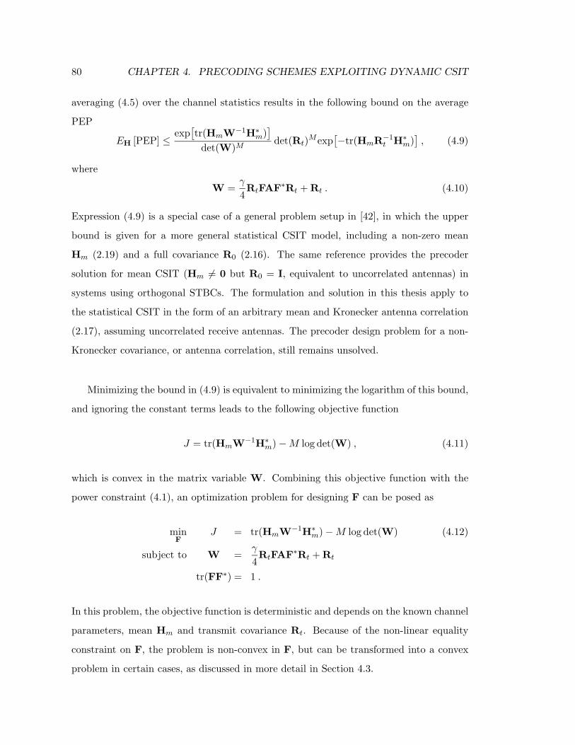
80 CHAPTER 4. PRECODING SCHEMES EXPLOITING DYNAMIC CSIT
averaging (4.5) over the channel statistics results in the following bound on the average
PEP
EH [PEP] ≤ exp[
tr(HmW−1H∗m)
]
det(W)Mdet(Rt)
Mexp[
−tr(HmR−1t H∗
m)]
, (4.9)
where
W =γ
4RtFAF∗Rt + Rt . (4.10)
Expression (4.9) is a special case of a general problem setup in [42], in which the upper
bound is given for a more general statistical CSIT model, including a non-zero mean
Hm (2.19) and a full covariance R0 (2.16). The same reference provides the precoder
solution for mean CSIT (Hm 6= 0 but R0 = I, equivalent to uncorrelated antennas) in
systems using orthogonal STBCs. The formulation and solution in this thesis apply to
the statistical CSIT in the form of an arbitrary mean and Kronecker antenna correlation
(2.17), assuming uncorrelated receive antennas. The precoder design problem for a non-
Kronecker covariance, or antenna correlation, still remains unsolved.
Minimizing the bound in (4.9) is equivalent to minimizing the logarithm of this bound,
and ignoring the constant terms leads to the following objective function
J = tr(HmW−1H∗m) − M log det(W) , (4.11)
which is convex in the matrix variable W. Combining this objective function with the
power constraint (4.1), an optimization problem for designing F can be posed as
minF
J = tr(HmW−1H∗m) − M log det(W) (4.12)
subject to W =γ
4RtFAF∗Rt + Rt
tr(FF∗) = 1 .
In this problem, the objective function is deterministic and depends on the known channel
parameters, mean Hm and transmit covariance Rt. Because of the non-linear equality
constraint on F, the problem is non-convex in F, but can be transformed into a convex
problem in certain cases, as discussed in more detail in Section 4.3.

4.2. PRECODING DESIGN CRITERIA 81
Average PEP criterion
Another formulation is obtained by averaging the PEP over both the codeword distribu-
tion and the fading statistics. This average PEP criterion is independent of the specific
codeword distance A.
For the system in Figure 4.1, assuming the input code is Gaussian distributed with
zero mean, it has a normalized-covariance as
Q =1
TPE[CC∗] , (4.13)
where T is the code length in number of symbols. The average codeword distance (4.7),
assuming that C and C are independent, then becomes
A =1
TP
(
E[CC∗] + E[CC∗])
= 2Q . (4.14)
After averaging over the codeword distribution, the Chernoff bound on the PEP (4.3)
depends only on the codeword covariance matrix Q as [71]
EC [PEP] ≤ det(γ
2HFQF∗H∗ + I
)−M.
The precoder optimization problem in this case becomes
minF
EH
[
det(γ
2HFQF∗H∗ + I
)−M]
(4.15)
subject to tr(FF∗) = 1 .
This formulation aims at finding the precoder F to minimize the Chernoff bound on
the PEP, averaged over all codeword distances and the channel statistics, subject to the
transmit power constraint.
4.2.2 The system capacity measure
The ergodic capacity criterion aims at maximizing the transmission rate with vanishing er-
ror, assuming asymptotically long codewords. Given dynamic CSIT, the capacity-optimal

82 CHAPTER 4. PRECODING SCHEMES EXPLOITING DYNAMIC CSIT
signal is zero-mean Gaussian-distributed with an optimal covariance. For the system in
Figure 4.1, assuming the predetermined input code is Gaussian distributed with covari-
ance Q (4.13), the transmit signal covariance is then FQF∗. With Gaussian additive
noise, the mutual information between the channel input and output can be obtained
explicitly as [46]
I(X, Y ) = log det(I + γHFQF∗H∗) ,
where γ is the SNR. The system ergodic-capacity and optimal signal are established by
maximizing this mutual information, subject to the transmit power constraint as
max EH
[
logdet(I + γHFQF∗H∗)]
(4.16)
subject to tr(FF∗) = 1 .
If the encoder in Figure 4.1 produces i.i.d. codewords so that Q = I, the above formulation
coincides with the channel information capacity discussed in Chapter 3. Otherwise, it
provides the system capacity. Subsequently, this formulation is referred to as the capacity
criterion.
For both the capacity (4.16) and the average-PEP (4.15) criteria, the objective func-
tion involves an expectation that has no closed-form. The function under expectation is
concave (or convex) in the Hermitian PSD matrix variable HFQF∗H∗. Depending on Q,
the problems can be transformed to be convex. These formulations belong to a class of
stochastic optimization problems, which also includes the error-exponent and the MMSE
criteria [19]. Problems in this class have similar solvability and are discussed in Section
4.5.
4.3 Optimal precoders based on the PEP per-distance
This section discusses precoder solutions based on the PEP per-distance criterion (4.12).
Because of the non-linear power constraint, this problem is not convex in F and, hence,
is not directly tractable in the original variable F. The tractability of this problem
is dependent on the structure of the matrix A, which in turn depends on the STBC.

4.3. OPTIMAL PRECODERS BASED ON THE PEP PER-DISTANCE 83
STBCs can be divided into two categories: orthogonal and non-orthogonal. Section 4.3.1
considers precoder design with orthogonal STBC, which lends an attractive property to
A. Section 4.3.2 then extends the analysis to general STBCs.
4.3.1 Precoder design with orthogonal STBC
Consider precoding with orthogonal STBC (OSTBC) [17]. Because of orthogonality, the
distance product matrix (4.4) of an OSTBC has a special form
A =1
P(C − C)(C − C)∗ = µI,
where µ represents the codeword distance, dependent on the specific codeword pair.
Let µ0 be the value corresponding to the matrix A chosen for the precoder optimiza-
tion problem. Based on the design choice (Section 4.2.1), µ0 can be either the minimum
or the average distance over all distinct-codeword pairs. The numerical simulation section
(Section 4.3.3) provides examples of how µ0 is calculated in each case.
A scaled-identity matrix A helps to significantly simplify the optimization problem
(4.12). The variable W is now a linear function of FF∗, and (4.12) becomes
minF
J = tr(HmW−1H∗m) − M log det(W) (4.17)
subject to W =µ0γ
4RtFF∗Rt + Rt
tr(FF∗) = 1 .
Denote η0 = 14µ0γ. This problem can be cast in terms of W as follows:
minW
tr(HmW−1H∗m) − M log det(W) (4.18)
subject to tr(R−1t WR−1
t − R−1t ) = η0
R−1t WR−1
t − R−1t < 0 ,
where the inequality results from the positive semi-definite (PSD) property that FF∗ < 0.
Formulation (4.18) is convex in the matrix variable W and can be solved analytically.

84 CHAPTER 4. PRECODING SCHEMES EXPLOITING DYNAMIC CSIT
Problem analysis
Problem (4.18) is now analyzed using the Lagrangian dual method [54]. Let Φ be the
following function of W:
Φ(W) = R−1t WR−1
t − R−1t , (4.19)
then the two constraints in (4.18) can be rewritten in terms of Φ as
tr(Φ) = η0 (4.20)
Φ < 0 . (4.21)
Form the Lagrangian of (4.18) as
L(W, ν,Z) = tr(HmW−1H∗m) − M log det(W) + ν [tr(Φ) − η0] − tr(ZΦ) , (4.22)
where ν is the Lagrange multiplier associated with the equality constraint (4.20), and Z <
0 is the Lagrange multiplier in the matrix form associated with the inequality constraint
(4.21). Strong duality holds for problem (4.18), easily verifiable using Slater’s condition
[54]. This condition requires the existence of a strictly feasible point: a positive definite
matrix Φ0 Â 0 satisfying the equality constraint (4.20). An example is Φ0 = η0I/N .
Therefore, the primal and dual optimal-points of (4.18) satisfy the Karush-Kuhn-Tucker
(KKT) conditions [54]
tr(Φ?) = η0
Φ? < 0
Z? < 0
tr(Z?Φ?) = 0
∂L(W, ν,Z)
∂W
∣
∣
∣
∣
W?,ν?,Z?
= 0 ,
where (.)? denotes the optimal value, and Φ? is the value of Φ evaluated at the optimal
W?.
In particular, the three conditions Φ? < 0, Z? < 0, and tr(Z?Φ?) = 0 imply that all

4.3. OPTIMAL PRECODERS BASED ON THE PEP PER-DISTANCE 85
eigenvalues of the positive semi-definite product Z?Φ? are zero. Thus, Φ? and Z? must
have the same eigenvectors, and their eigenvalue patterns are complementary; that is,
if λi(Φ?) > 0, then λi(Z
?) = 0 and vice-versa. Z effectively ensures that Φ is positive
semi-definite: Z represents the eigen-modes that are dropped in a water-filling solution,
whereas Φ represents the modes that are active (with non-zero power). Therefore, if
power is distributed over the correct number of positive eigenvalues of Φ, while the rest
are set to zero, then in the Lagrangian (4.22), the term tr(ZΦ) is automatically zero at the
optimal values and, hence, can be ignored. From this observation, a two-step algorithm
for solving problem (4.18) is outlined below.
Precoding design algorithm
In the first step, assume that the optimal Φ? is full-rank, effectively ignoring the PSD
inequality constraint (4.21), and solve for W. If the solution of this step produces Φ < 0,
then it is also the solution for the original problem (4.18). The matrix Φ becomes the
scaled precoder-product η0FF∗, which is full-mode in this case. However, if the solution
of the first step does not produce a PSD Φ, then the algorithm proceeds to the second
step. In this step, the weakest eigenvalue of Φ is set to zero, effectively reducing the rank
of Φ by 1, and the problem is re-solved. This step is iterated until Φ is PSD. The second
step is equivalent to dropping a mode in a water-filling process. In both steps, finding
the solution for Φ essentially reduces to solving for the Lagrange multiplier ν, as detailed
next.
By ignoring tr(ZΦ) in the Lagrangian (4.22), the optimality condition is obtained by
differentiating this Lagrangian with respect to W [60] to arrive at
−W−1H∗mHmW−1 − MW−1 + νR−2
t = 0 . (4.23)
This is a quadratic matrix equation. Solving this equation leads to the solution for W as
W =1
2νRt
(
MIN + Ψ1
2
)
Rt , (4.24)

86 CHAPTER 4. PRECODING SCHEMES EXPLOITING DYNAMIC CSIT
where
Ψ = M2IN + 4νR−1t H∗
mHmR−1t . (4.25)
The derivation is given in Appendix A.3. From the above solution for W, the solution
for Φ can be established according to (4.19).
It is left to find the Lagrange multiplier ν, based on the transmit-power equality
constraint (4.20). The algorithm for solving for ν in each of the two steps is given below.
Step 1. Full-mode solution
The full-mode solution is obtained by solving for ν, assuming Φ is full-rank. Equa-
tion (4.20) can then be written as
tr( 1
2ν
(
MIN + Ψ1
2
)
− R−1t
)
= η0 . (4.26)
Let λi (i = 1 . . . N) be the eigenvalues of R−1t H∗
mHmR−1t , sorted in increasing
order, β0 = 2[
tr(
R−1t
)
+ η0
]
, and noting that λ (aI + A) = a + λ(A), the above
equation becomes
MN +N
∑
i=1
√
M2 + 4νλi − β0ν = 0 . (4.27)
In the general case (N > 1), this equation does not appear to have a closed-form
solution. Nevertheless, solving for ν can be done efficiently using a binary search,
called the “inner algorithm”, as outlined below.
Inner algorithm.
Since the left-hand-side expression in (4.26) is monotonous in ν, the following lower
and upper bounds on the solution for ν can be established:
νlower =4N2λ1
β20
+2MN
β0, νupper =
4Nα0
β20
+2MN
β0, (4.28)
where λ1 is the minimum eigenvalue and α0 is the trace of R−1t H∗
mHmR−1t . The
lower bound is obtained from (4.27) by replacing all λi with λ1, while the upper
bound by applying the Cauchy-Schwartz inequality [72] to the summation term. A
numerical binary search can then be performed between these bounds to find the

4.3. OPTIMAL PRECODERS BASED ON THE PEP PER-DISTANCE 87
solution for (4.27) up to a desired precision. The number of iterations depends
on the problem parameters, but convergence usually occurs rapidly since this is
one-dimensional binary search.
Step 2. Mode-dropping solution
If the full-mode solution does not produce Φ < 0, then the weakest eigen-mode of
Φ is dropped and (4.26) is re-solved for ν. This step is equivalent to a water-filling
iteration. The total power will now be distributed over the N−1 largest eigenvalues
of Φ, and the power constraint (4.26) changes to
N∑
i=k+1
λi
( 1
2ν
(
MIN + Ψ1/2)
− R−1t
)
= η0 , (4.29)
where k = 1, the number of modes dropped, and λi(·) is the ith eigenvalue of the
matrix in the parenthesis, sorted in increasing order (λ1 ≤ · · · ≤ λN ). The solution
for Φ is obtained after solving this equation for ν, forming the right-hand-side
expression in (4.19), and forcing its smallest eigenvalue to be zero, after which, it
satisfies (4.20). If this solution does not satisfy (4.21), then the number of dropped
modes k is increased by 1, and (4.29) is re-solved. Again, the above equation does
not have a closed-form solution, but can be solved using an efficient binary search,
called the “outer algorithm”, as described below.
Outer algorithm.
There is no explicit function relating the eigenvalues of a general matrix sum to
the individual eigenvalues; therefore, each eigenvalue in (4.29) cannot be written
as an explicit function of ν (except in the special cases discussed in Section 4.4.3).
Fortunately, the sum of eigenvalues in (4.29) is monotonous in ν, allowing the
derivation of upper and lower bounds on ν. A binary search can then be performed
to efficiently find the solution between these two bounds up to any desired numerical
precision. The bounds in the general case with k modes dropped (1 ≤ k ≤ N − 1)
are
νupper =λN
β2k
+M
βk, νlower =
λ1
β2k
+M
βk, (4.30)

88 CHAPTER 4. PRECODING SCHEMES EXPLOITING DYNAMIC CSIT
where λN and λ1 are the maximum and the minimum eigenvalues of R−1t H∗
mHmR−1t ,
respectively, and
βk =1
N − k
(
η0 +N
∑
i=k+1
1
λi(Rt)
)
.
The derivation of these bounds is given in Appendix A.4.
Dynamic water-filling
The mode-dropping process above is similar to the water-filling process, in that at each
outer iteration, an eigen-mode (the weakest among the active modes) is dropped, and
the total transmit power is re-allocated over the rest of the modes. There is, however, a
significant difference between this process and the conventional water-filling process. In
conventional water-filling, only the power allocation, or the water level, changes after each
iteration, but the mode directions remain the same. In our problem, the mode directions
also evolve at each iteration, because of the interaction of the channel mean and the
transmit covariance matrices. To see this effect more clearly, rewrite the expression for
Φ in the following form:
Φ =M
2νIN +
(
1
2νΨ(ν)
1
2 − R−1t
)
,
where the notation Ψ(ν) emphasizes the dependence of Ψ on ν. The “water-level” here
is M/2ν, and the mode directions are determined by the eigenvectors of the matrix
expression inside the large parenthesis, in which Ψ and Rt have different eigen-directions.
When ν changes at each outer iteration, both the water-level (hence, the power allocation)
and the mode directions change. Moreover, since the ν solution depends on the SNR,
both the precoder power allocation and mode (beam) directions are functions of the SNR.
For this reason, this process is called dynamic water-filling.

4.3. OPTIMAL PRECODERS BASED ON THE PEP PER-DISTANCE 89
The optimal precoder solution with scaled-identity A
When ν is found satisfying the PSD constraint (4.21), then the matrix Φ provides the
solution for FF∗ as
Φ =1
2ν
(
MIN + Ψ1
2
)
− R−1t = η0FF∗ . (4.31)
From this product expression, an optimal precoder can be derived. The optimal precoder
is not unique. Let the eigenvalue decomposition of Φ be
Φ = UΦΛΦU∗Φ ,
then, in terms of the singular value decomposition, the optimal precoder matrix is
F =1√η0
UΦΛΦ1/2V∗ . (4.32)
The left singular vectors and the singular values of an optimal precoder are the eigenvec-
tors and the scaled square-roots of the eigenvalues of Φ, respectively. The right singular
vectors V, however, can be any unitary matrix, attributed to the codeword distance
product matrix A being scaled-identity. For simplicity, set V = I for a precoder with
scaled-identity A.
Summary on precoding with OSTBC
By solving a convex optimization problem with matrix variables, this section has estab-
lished an analytical design algorithm for a precoder used with an orthogonal STBC. The
algorithm resembles the water-filling process. At first, it is assumed that all precoder
eigen-modes are active, and power allocation is performed on all modes. If any mode
has negative power, that mode is dropped, and the power is re-allocated accordingly.
During this process, the precoder eigen-beam directions also evolve with the water-filling
iterations. Each iteration essentially aims at finding a Lagrange multiplier solution, us-
ing an efficient binary search. The algorithm produces the optimal beam directions, or
the precoder left singular vectors, and the optimal beam power allocation. The precoder
right singular vectors, however, can be arbitrary, due to the isotropic property of the

90 CHAPTER 4. PRECODING SCHEMES EXPLOITING DYNAMIC CSIT
orthogonal STBC, and are usually omitted.
4.3.2 Precoder design with general STBC
This section examines (4.12) when the codeword distance product matrix A (4.4) results
from any STBC. For a non-orthogonal STBC, A is not always a scaled-identity matrix.
Since the scaled-identity A case was solved in Section 4.3.1, this section focuses on solving
for the non-identity A next, then discusses the precoder solution with general STBC in
Section 4.3.2.
Problem analysis for a non-identity codeword distance product
When A is not a scaled-identity matrix, the optimization problem (4.12) is non-convex
and more difficult. In particular, due to the non-convexity, it is not obvious if the problem
can be solved exactly. This section analyzes and reformulates the problem, then applies
different relaxations to obtain a precoder analytically.
To analyze (4.12) for a non-identity A, consider the following more constrained prob-
lem:
minF
J = tr(
HmW−1H∗m
)
− M log det(W) (4.33)
subject to W =γ
4RtFAF∗Rt + Rt
tr(FF∗) = 1
tr(FAF∗) = p ,
where p is a positive constant. Since this problem is more constrained than the original
problem (4.12), its optimal J value will be larger than, or equal to, the optimal J value
in (4.12). The smallest optimal J value in (4.33) across different p values, however, will
equal the optimal J value in (4.12), at which point, the two problems become equivalent.
Now consider problem (4.33) with different p values. In this problem, the condition
tr(FAF∗) = p acts as an additional transmit power constraint. Obviously, with more
transmit power, the error probability, or the objective function J equivalently, will be
smaller. Of interest is the problem with the largest feasible p; that is, the largest p

4.3. OPTIMAL PRECODERS BASED ON THE PEP PER-DISTANCE 91
value such that there exists an F satisfying both equality constraints, tr(FF∗) = 1 and
tr(FAF∗) = p.
Applying the matrix inequality tr(AB) ≤ ∑
i λi(A)λi(B) for PSD matrices [73] to
obtain
p = tr(FAF∗) = tr(F∗FA) ≤∑
i
λi(F∗F)λi(A). (4.34)
The equality occurs when the eigenvectors of F∗F are the same as those of A. Consider
the SVD of the precoder F = UFDV∗F as in (1.4), this equality condition means
VF = UA , (4.35)
where A = UAΛAU∗A is the eigenvalue decomposition of A. Since the eigenvalues of
F∗F are the same as those of FF∗, the equality condition translates to λi(FAF∗) =
λi(FF∗)λi(A).
Condition (4.35) ensures the largest value for p, without imposing any constraint on
the eigenvalues of FAF∗ or FF∗, except their orders relative to λi(A). With this condi-
tion, problem (4.33) and the original problem (4.12) become equivalent when p is chosen
to be the same as that resulted from the optimal solution of (4.12): p =∑
i λi(A)λ?i (FF∗).
Based on these arguments, condition (4.35) is optimal for the original problem (4.12).
Let B = FAF∗, this problem is then equivalent to
minB
J = tr(
HmW−1H∗m
)
− M log det(W) (4.36)
subject to W =γ
4RtBRt + Rt
∑
i ξiλi(B) = 1
B < 0 ,
where ξi = [λi(A)]−1 are the inverses of the non-zero eigenvalues of A.
By finding the optimal right singular vectors of F in (4.35), the original problem (4.12)
has been reformulated into a new problem (4.36) in terms of the variable B. This new
formulation, however, is not convex in B, because of the non-linear equality constraint
involving the eigenvalues of B. Next, this constraint is relaxed to obtain an analytical

92 CHAPTER 4. PRECODING SCHEMES EXPLOITING DYNAMIC CSIT
precoder solution. Because of relaxation, the solution in this case may not be optimal for
the original problem. Two different relaxations follow.
Minimum eigenvalue relaxation method
Employing the inequality∑
i ξiλi(B) ≤ ξmaxtr(B), the problem can be relaxed by replac-
ing all ξi with ξmax, which is equivalent to approximating A in (4.12) with an identity
matrix, scaled by the minimum non-zero eigenvalue of A. This approximation effectively
produces a smaller W (in the positive semi-definite sense), hence loosening the upper-
bound on the PEP in (4.9). This relaxation results in the same problem formulation as
in the orthogonal STBC case (4.17), where the value µ0 for the minimum-distance design
is
µ0 = min∆ij
λmin(∆ij∆∗ij) ,
and for the average-distance design is µ0 = λmin(A) (with λmin 6= 0). This relaxation
method works well if the condition number of A is reasonably small.
Trace relaxation method
Another relaxation method is to replace the equality constraint on the eigenvalues of B
with the linear constraint tr(Λ−1A B) = 1, making the relaxed problem convex. Based on
the inequality tr(AB) ≥ ∑
i λN−i+1(A)λi(B) for ordered eigenvalues of Hermitian PSD
matrices [72], this relaxation method results in a precoder with tr(FF∗) ≤ 1, meaning
that the total transmit power may be less than the original constraint (4.1). A scaling
factor can then be applied to the precoder solution of the relaxed problem to increase the
power to meet the original constraint.
Noting that B = 4γ
(
R−1t WR−1
t − R−1t
)
, reformulate the problem in terms of W as
minW
tr(
HmW−1H∗m
)
− M log det(W) (4.37)
subject to tr(
Λ−1A
(
R−1t WR−1
t − R−1t
))
=γ
4
R−1t WR−1
t − R−1t < 0 .
This problem is similar to (4.18), but with a more general trace constraint; it can be

4.3. OPTIMAL PRECODERS BASED ON THE PEP PER-DISTANCE 93
solved using a similar approach. The steps for solving this problem and the solutions for
W and B are given in Appendix A.5.
The precoder solution with general STBC
Returning to the general STBC case, if the codeword distance product matrix A is a
scaled-identity matrix, then the precoder solution is similar to that of the orthogonal
STBC case (4.32). For a non-identity A, employ one of the relaxation methods outlined
above and solve for B. Perform the eigenvalue decomposition of this matrix as B =
UBΛBU∗B, then the precoder solution is
F = UBΛ1
2
BΛ− 1
2
A U∗A . (4.38)
For an orthogonal STBC, since A is always a scaled-identity matrix, UA is an arbitrary
unitary matrix and, hence, can be omitted. For a non-orthogonal STBC, UA depends
on the STBC structure. Specifically, when A is not a scaled-identity matrix, the input
signal produced by the STBC has a certain codeword-error shape with directions UA
and power loadings λi(A). The precoder then matches both its input signal structure
and the channel. It effectively re-maps the input signal directions from UA into UB and
re-distributes the transmit power according to the CSIT to optimally match the channel.
Note that the precoder beam directions (the left singular vectors UB) depend only on
the CSIT; the input shaping matrix (the right singular vectors UA) depends only on the
precoder input signal – the STBC structure; and the power allocation now depends on
both sides.
Recall that the matrix A can be chosen based on the minimum- or the average-distance
criterion. Between these two criteria, the average-distance criterion usually produces a
scaled-identity matrix A, assuming equi-probability and independence between all input
symbols. The reason is that STBCs commonly assume no CSIT and distribute power
equally among all antennas and all symbols, leading to a white error-covariance. The
minimum-distance criterion, on the other hand, can often produce a non-identity A.

94 CHAPTER 4. PRECODING SCHEMES EXPLOITING DYNAMIC CSIT
Summary on precoding with general STBC
This section has extended the precoder design algorithm in Section 4.3.1 to cover pre-
coding with non-orthogonal STBC. In contrast to the isotropic property of an orthogonal
STBC, a non-orthogonal STBC may pre-shape the input signal with a non-identity code-
word distance product matrix A. In that case, the precoder optimal right singular vectors
are given by the eigenvectors of A. For a non-identity A, relaxations are used to find the
precoder left singular vectors and the singular values. In general, the precoder solution
contains matching singular vectors on each side to the STBC structure and to the channel
respectively, while the singular values depend on both the STBC and the CSIT. The pre-
coder essentially re-maps the spatial directions of the input signal to match those of the
channel, based on the CSIT, and allocates transmit power accordingly in a water-filling
fashion.
4.3.3 Design examples and performance results
This section shows design examples and simulation results for several system configura-
tions, using two antenna setups: 2 × 1 and 4 × 1. The channel mean and transmit co-
variance matrices are generated arbitrarily and normalized according to Appendix B.1, in
which the covariance matrix is Hermitian and positive definite. These matrices are given
in Appendix B.3. The covariance matrix for the 2 × 1 channel has the eigenvalues as
[1.96, 0.04] and the condition number of 47.93, representing a strong antenna correlation.
The covariance matrix for the 4×1 channel has the eigenvalues as [2.05, 1.48, 0.41, 0.06]
and the condition number of 34.2. In all systems, the K factor is chosen to be 0.1, except
when studying the effect of K on the precoder.
Precoders with orthogonal STBC
This section first discusses a design example for precoding with the Alamouti STBC [74],
which is capacity-optimal for a 2 × 1 system, then presents error-rate simulation results.

4.3. OPTIMAL PRECODERS BASED ON THE PEP PER-DISTANCE 95
The Alamouti STBC is given as
C =
c1 −c∗2
c2 c∗1
,
where ci are symbols from a chosen constellation.
Codeword distance of the Alamouti STBC
The value for µ0 in (4.17) is established as follows. For the minimum-distance design, A =
d2
P I, where d is the minimum distance in the signal constellation. Consider a square QAM
constellation with Mc points for example, the average symbol power is P = d2(Mc−1)/6,
thus µ0 = 6/(Mc − 1).
For the average-distance design, assuming that each codeword contains n distinct
symbols that are independent and equally likely, the codeword distance product matrix
(4.7) can be rewritten as
A =1
TPE
C6=C
[
(
C − C)(
C − C)∗
]
=1
TP
M2nc
M2nc − Mn
c
2(
E[
CC∗]
− E[
CC∗]
)
, (4.39)
where the ratio factor results from averaging over only pairs of distinct codewords. This
expression applies to any signal constellation of size Mc. Since C and C are chosen
independently, E[CC∗] = 0. For a STBC that gives equal weight to all symbols, it is
plausible that E[CC∗] = µP I for some µ. Hence, the average-distance criterion usually
produces a scaled-identity matrix A. For the Alamouti code with QPSK, for example,
A = 6415I, or µ0 = 4.26.
Numerical results
Figure 4.2(a) shows the performance of a 2×1 system using the Alamouti code and QPSK
modulation. For this system, the minimum-distance and the average-distance precoders
perform exactly the same. The precoding gain is around 2.2dB at low and medium SNRs
and diminishes at higher SNRs. When the SNR increases, as discussed in Section 4.4.2,
the precoder becomes increasingly dependent on the transmit covariance and approaches

96 CHAPTER 4. PRECODING SCHEMES EXPLOITING DYNAMIC CSIT
−4 −2 0 2 4 6 8 10 12 14 1610
−3
10−2
10−1
100
Bit error probability
Codeword error probability
PEP bound
SNR in dB
Cod
ewor
d an
d bi
t err
or p
roba
bilit
ies
PEP bound no prec.PEP bound with prec.No precoderMininum dist. precoderAverage dist. precoder
(a)
−5 0 5 10 15 20 25 30 3510
−3
10−2
10−1
100
QPSK
16QAM
64QAM
SNR in dB
Cod
ewor
d er
ror
prob
abili
ty
No precoderAverage dist. precoderMininum dist. precoder
(b)
Figure 4.2: Performance of a 2×1 system with and without precoding, using the Alamouticode and (a) QPSK modulation, (b) various QAMs.
equi-power on the non-zero eigen-modes of A. With OSTBC, the matrix A is always full-
rank; thus, the value of water-filling power allocation decreases at a high SNR, leading to
the diminishing precoding gain.
Figure 4.2(b) shows the performance for the same 2 × 1 system with different QAM
orders. The precoding gain of the minimum-distance design is consistent over different
constellation sizes, whereas the average-distance precoding gain is reduced with larger
constellation at high SNRs. With a larger constellation, the number of minimum-distance
codeword pairs becomes larger, while at a higher SNR, the minimum-distance pairs be-
come more dominant in affecting the error probability. Therefore, the minimum-distance
precoder design results in more gain than the average-distance design in this domain.
Precoders with non-orthogonal STBC
This section continues with an example of a linear precoder design with non-orthogonal
STBC. This example uses the quasi-orthogonal STBC (QSTBC) [75, 76] specifically. The
name quasi-orthogonal results from the groups of columns of this code being orthogonal
to each other, allowing simple ML decoding over pairs of symbols. The code itself is
non-orthogonal and provides partial diversity; however, it achieves a higher rate than
an OSTBC for more than two transmit antennas. Consider the following form of the

4.3. OPTIMAL PRECODERS BASED ON THE PEP PER-DISTANCE 97
QSTBC:
C =
c1 c2 c3 c4
−c∗2 c∗1 −c∗4 c∗3
c3 c4 c1 c2
−c∗4 c∗3 −c∗2 c∗1
, (4.40)
where ci are symbols from a chosen constellation C. In [66], a precoder exploiting mean
CSIT in a system with the QSTBC is derived, using an asymptotic analysis.
The codeword distance product matrix for the QSTBC
For this code, the codeword distance product matrix A (4.4) has the form
A =1
P
a 0 b 0
0 a 0 b
b 0 a 0
0 b 0 a
,
where a =∑4
i=1 |∆ci|2 and b = ∆c1∆c∗3+∆c∗1∆c3+∆c2∆c∗4+∆c∗2∆c4, with ∆ci = ci− ci,
where ci are symbols in C.
For the minimum-distance design, A is given by the case in which there is only one
symbol difference between the two codewords, thus Amin = minC(|∆c|2)I/P . For the
average-distance design, assuming that all symbols ci are independent and equally likely,
and that E[ci] = 0, A (4.39) is also a scaled-identity matrix with µ0 = 2M8c /(M8
c −M4c ). In
this QSTBC example, A is a scaled-identity matrix in both designs; hence, no relaxation
is needed to solve for the precoder, and the precoder right singular vectors can be omitted.
Although the STBC diversity order, or the minimum rank of A, is 2 in this case, the
precoder is not limited to rank 2. At each time instance, the precoder acts as a beamformer
on a separate column of the space-time code. Since there are 4 different symbols in each
column, the precoder can form a maximum of four orthogonal beams, one per symbol,
matching the statistically preferred directions in the channel. This beamforming effect
causes the precoder rank to be independent of the STBC diversity order. Rather, it
depends on the number of different symbols in each column of the code. Only when the

98 CHAPTER 4. PRECODING SCHEMES EXPLOITING DYNAMIC CSIT
0 5 10 15 20 25
10−5
10−4
10−3
10−2
10−1
100
Bit error probability
Codeword error probability
SNR in dB
Cod
ewor
d an
d bi
t err
or p
roba
bilit
ies
No precoderRank ≤ 2 precoderAverage dist. precoderMininum dist. precoder
(a)
5 10 15 20 25 3010
−5
10−4
10−3
10−2
10−1
100
Codeword error probability
Bit error probability
SNR in dB
Cod
ewor
d an
d bi
t err
or p
roba
bilit
ies
No precoderRank ≤ 2 precoderAverage dist. precoderMinimum dist. precoder
(b)
Figure 4.3: Performance of a 4×1 system with and without precoding, using the QSTBCand (a) QPSK modulation, (b) 16 QAM.
SNR is not high enough, the precoder reduces its rank by dropping modes.
Numerical results
Figure 4.3(a) shows the performance curves for a 4 × 1 system using the QSTBC and
QPSK modulation. The result reveals that both the minimum-distance and the average-
distance precoder designs perform similarly for the QPSK modulation, with a precoding
gain of around 1.7dB – 2dB. Also shown is the performance of a precoder that has its
rank limited to 2. This precoder gain reduces rapidly as the SNR increases; it eventually
performs even worse than without precoding at very high SNRs. This example illustrates
that the precoder rank should not depend on the STBC diversity order.
Figure 4.3(b) shows similar performance curves for the 16QAM constellation with
Gray bit-mapping. In this case, the minimum-distance precoder design performs slightly
better than the average-distance design, due to the larger constellation at high SNRs
effect, which is also observed in Figure 4.2(b). The difference is small, however, at around
0.5dB. With this larger constellation, the precoding gain is higher; the minimum-distance
precoding gains are around 1.8 – 2.5dB.

4.3. OPTIMAL PRECODERS BASED ON THE PEP PER-DISTANCE 99
−4 −2 0 2 4 6 8 10 12 1410
−5
10−4
10−3
10−2
10−1
SNR in dB
BE
R, p
reco
ding
= s
olid
No precoderρ = 0ρ = 0.8ρ = 0.9ρ = 0.96ρ = 0.99
(a)
0 0.2 0.4 0.6 0.8 110
−4
10−3
10−2
10−1
Channel estimate quality ρ
BE
R, p
reco
ding
= s
olid
SNR = 2dBSNR = 6dBSNR = 10dBNo Precoding
(b)
Figure 4.4: Performance of the minimum-distance PEP precoder in a 4 × 1 system withOSTBC, given dynamic CSIT.
Precoding with dynamic CSIT
The precoding designs (4.32) and (4.38) can be applied directly to dynamic CSIT, using
the effective channel mean H (2.25) and the effective transmit covariance Rt,e (2.27) in the
place of the channel statistics. This section considers the performance of a 4 × 1 system,
given dynamic CSIT. The channel parameters, mean and transmit covariance, are the
same as in the simulation for Figure 4.3, as given in Appendix B.3. This system, however,
employs a rate 3/4 orthogonal STBC for 4 transmit antennas [17]. The error performance
is averaged over multiple initial channel measurements, independently generated from the
channel distribution, and multiple channel estimates given each initial measurement.
Figure 4.4(a) shows the system bit-error-rate (BER) given different CSIT qualities
ρ. The performance improves with higher ρ. When ρ = 0, the precoding gain is that of
statistical CSIT alone. As ρ → 1, the gain increases to a maximum of 6dB, which is the
maximum coding gain possible from perfect CSIT for a 4 × 1 channel.
Figure 4.4(b) presents the BER as a function of the CSIT quality ρ at different SNRs.
This result shows that the gain is sensitive to ρ only when ρ ≥ 0.6, at which dynamic
CSIT has an advantage over statistical CSIT. This observation implies that the initial
channel measurement helps to increase the precoding gain only when its correlation with
the current channel is reasonably strong, ρ ≥ 0.6 in this case; otherwise, precoding on the

100 CHAPTER 4. PRECODING SCHEMES EXPLOITING DYNAMIC CSIT
−4 −2 0 2 4 6 8 10 12 1410
−4
10−3
10−2
10−1
SNR in dB
BE
R (
prec
odin
g =
sol
id)
No precoderρ = 0ρ = 0.8ρ = 0.9ρ = 0.99H
0 beamforming
Figure 4.5: Performance comparison between the minimum-distance PEP precoder andthe beamforming scheme relying only on outdated channel measurements.
channel statistics alone (ρ = 0) can extract most of the gain.
The precoder is compared with a beamforming scheme that uses only the initial chan-
nel measurement H0 as shown in Figure 4.5. With perfect CSIT (numerically represented
by ρ = 0.99), these two schemes coincide and are optimal for a 4×1 MISO channel. How-
ever, as ρ decreases, the H0 beamforming scheme starts loosing diversity at high SNRs
and eventually performs even worse than without precoding. The precoder exploiting
dynamic CSIT, on the other hand, provides gains over no precoding for all ρ values. This
result illustrates the robustness of the dynamic CSIT model.
4.4 Analyses of PEP-based precoders
This section analyzes the precoding design based on the PEP per-distance criterion, de-
rived in the previous section. The analyses include the precoding gain, asymptotic pre-
coders with increasing K factor and SNR, and precoders for special scenarios: transmit
covariance CSIT and mean CSIT.
4.4.1 The precoding gain
The precoding gain can include two components: diversity and coding. The diversity
gain refers to an increase in the asymptotic slope of the error rate curve vs the SNR as

4.4. ANALYSES OF PEP-BASED PRECODERS 101
the SNR increases to infinity. The coding gain, on the other hand, refers to an SNR
advantage, corresponding to a parallel shift of the error rate curve to lower SNRs with
the same asymptotic slope. Coding gains can be measured at a finite SNR.
Diversity gain
Diversity is a high-SNR measure, obtained as the dominant exponent of the error prob-
ability expressed in terms of the SNR. Specifically, the system diversity order is defined
as
d = limSNR→∞
log10
(
Pe
)
log10(SNR),
where Pe is the average system error probability. The system diversity can also be ob-
tained from the exponent of the maximum PEP [70, 71]. Since the Chernoff bound on the
PEP is asymptotically tight at high SNR, this diversity order can be derived by examining
the Chernoff bound (4.3) while taking γ → ∞.
For partial CSIT (ρ < 1), the effective transmit covariance is non-zero. The Chernoff
bound (4.3) can be averaged over the effective channel statistics to obtain (4.9). Noting
that only W depends on γ, the system diversity order can be derived from this averaged
bound as
d = limγ→∞
−tr
(
HW−1H∗)
− M log det(W)
log γ.
From (4.10), as γ → ∞ then W−1 → 0; thus, the trace term in the above expression
vanishes, and the diversity order becomes
d = limγ→∞
M log det(W)
log γ. (4.41)
As γ → ∞, the precoding solution (4.38) approaches a precoder with equi-power allocation
on the non-zero eigen-modes of A, and the left and right singular vectors given by the
eigenvectors of Rt and A, respectively (see Section 4.4.2, equ.(4.48)). Thus at high SNR,
W (4.10) approaches
Wγ limit =γ
4LUtΛ
2tΛAUt , (4.42)
where L is the minimum number of non-zero eigenvalues of A, determined by the diversity

102 CHAPTER 4. PRECODING SCHEMES EXPLOITING DYNAMIC CSIT
order of the STBC. The rank of Wγ limit is L. Thus, the system diversity order in (4.41)
is ML. Therefore, with partial CSIT, the precoder and the CSIT quality ρ have no
impact on the system diversity. With optimal ML detection, the system diversity is
solely determined by the STBC.
For perfect CSIT (ρ = 1), the Chernoff bound (4.3) can be used directly to de-
rive the optimal precoder and the diversity order. The optimal precoder is single-mode
beamforming on the dominant eigen-mode of H∗H (see Section 4.4.2, equ.(4.44)). This
precoder achieves the maximum diversity order of MN (see [7], Section 5.4.4). The proof
is based on loosening the bound (4.3), by replacing A with Iλmax(A) and using no pre-
coder (F = 1/√
N I); this relaxed bound has the diversity order MN . Thus, the precoder
for perfect CSIT achieves the full diversity, regardless of the STBC.
The above analysis shows that the diversity obtained by the precoder depends on
the CSIT. When the CSIT is partial, no diversity can be extracted by the precoder; the
STBC then plays an essential role in obtaining transmit diversity in the system. Only
when the CSIT is perfect that the precoder delivers the full transmit diversity. In all
cases, however, the precoder achieves a coding gain, as discussed next.
Coding gain
The coding gain is the essential value of precoding and comes in the form of an SNR
advantage. The simulation results in Section 4.3.3 illustrate that this gain depends on
the SNR, the CSIT, and the number of antennas. The gain is usually significant at low and
medium SNRs. It may diminish at high SNRs, depending on the system configuration,
such as in systems with OSTBC. The coding gain increases with higher CSIT quality ρ,
likewise with higher channel K factor. It also depends on the specific channel mean and
transmit covariance matrices. Some channels favor precoding with larger gains, while for
others, the gain is less significant. A variety of factors can contribute to this effect: for
example, the condition numbers of the mean and covariance matrices, how closely the
eigenvectors of these matrices align. This effect is not studied here and can be a subject
for further research. Furthermore, the number of antennas also affects the coding gain.
The gain tends to increase with increasing number of transmit antennas. Precoding on

4.4. ANALYSES OF PEP-BASED PRECODERS 103
a channel with the same transmit antenna correlation but with more receive antennas
also tends to produce a higher gain. Note that precoding with the focus on extracting an
array gain is fundamentally different from, and complementary to, achieving the diversity-
multiplexing frontier at high SNRs [71, 77, 78].
Summary on the precoding gain
The precoding gain is attributed to two factors: the optimal beam directions, which
achieve a coding gain from array beamforming, and the water-filling-type power allocation
among these beams, which also results in an SNR advantage. With partial CSIT (ρ < 1),
precoding on effective channel statistics obtains only coding gain, but not diversity gain.
This lack of diversity gain is a property of statistical channel information, in which the
precise directions of each channel realization are unknown to the transmitter. The STBC,
therefore, plays an important role in capturing the channel diversity here. When the CSIT
is perfect (ρ = 1), however, the precoder can also deliver the maximum diversity gain.
4.4.2 Asymptotic precoder results
This section analyzes several asymptotic behaviors of the optimal precoder based on
the PEP per-distance criterion. Two effects are studied: of the K factor and of the
SNR increasing to infinity. In each case, the precoder solution asymptotically depends
only on one of the two channel statistical parameters, either the mean or the transmit
covariance. These asymptotic precoder solutions are obtained in closed-form for all STBC
cases without relaxation.
The effect of a high K factor on the precoder
This section investigates the effect on the optimal precoder as the channel K factor
increases to infinity. An infinite K can correspond to a non-fading channel, or to perfect
instantaneous CSIT. In either case, it is useful to study this limit, so that applicable
scenarios can be identified.
When K approaches infinity, the objective function (4.11) is invalid since it also
approaches infinity; hence, the full upper-bound (4.9) is used. With the K factor, the

104 CHAPTER 4. PRECODING SCHEMES EXPLOITING DYNAMIC CSIT
channel model (2.18) can be written as
H =
√
K
K + 1Hm + Hw
√
1
K + 1R
1/2t ,
where Hm and Rt are normalized channel mean and transmit covariance as discussed in
Appendix B.1. The upper-bound (4.9) can then be re-written as
EH [PEP] ≤exp
[
tr(
KHmW−10 H∗
m
)]
det (W0)M
det(
Rt
)Mexp
[
−tr(
KHmR−1t H∗
m
)]
, (4.43)
where
W0 =γ
4(K + 1)RtFAF∗Rt + Rt .
Express W0 in the form W0 = R1/2t (Q + I) R
1/2t , where
Q =γ
4(K + 1)R
1
2
t FAF∗R1
2
t .
With sufficiently large K, the largest eigenvalue of the PSD Hermitian matrix Q will be
less than 1, and the following expansion [60] can be applied:
W−10 = R
− 1
2
t
(
I − Q + Q2 − Q3 + . . .)
R− 1
2
t .
Replacing this expression into the upper bound (4.43), and noting that
KW−10 − KR−1
0 → −γ
4FAF∗ as K → ∞,
the limiting upper bound on the average PEP is
PK limit = exp[
−tr(γ
4HmFAF∗H∗
m
)]
.
Minimizing PK limit is equivalent to maximizing the trace expression. Apply the in-
equality tr(ABC) ≤ ∑
i σi(A)σi(B)σi(C) [73] with σi(.) as sorted singular values, where
the equality is achieved when the right singular vectors of A (and B) align with the

4.4. ANALYSES OF PEP-BASED PRECODERS 105
left singular vectors of B (and C, respectively). Taking the power constraint (4.1) into
account, the optimal precoder F has the form
F = uv∗ , (4.44)
where u is the dominant eigenvector of H∗mHm and v is the dominant eigenvector of A.
In other words, the optimal precoder, in the limit of an infinite K factor, is a single-
mode beamformer, matching the dominant right singular vector of the channel mean.
This result applies regardless of the STBC or the choice of the minimum- or the average-
distance design, as the left singular vectors of F are independent of A.
For a multiple-input single-output (MISO) system at infinite K (or perfect channel
knowledge), single-mode beamforming is also optimal for achieving the channel capacity
[41]. Therefore, the proposed precoding solution is optimal for a MISO system in the
PEP criterion and asymptotically optimal in capacity. For a MIMO system, however,
the optimal solution in the limit of infinite K differs between the two criteria: PEP
per-distance and capacity. Whereas the capacity solution calls for water-filling over the
eigen-modes of the channel, the PEP solution places all transmit power on the dominant
mode. Thus, for a MIMO channel with high K factor, a precoder based on the PEP
per-distance criterion is suitable for use along with a STBC with a rate of one or less.
However, as K increases, the role of the STBC becomes less important in obtaining
diversity. Moreover, the power loading on the precoder dominant mode increases as K
increases; therefore, precoding can be combined with adaptive modulation and coding to
take the full advantage of high K. At a low K factor, due to the multi-mode beamforming
effect, a higher rate STBC can also be used with the PEP per-distance precoder in a
MIMO system.
High SNR precoder analysis
To analyze the effect of the SNR γ on the precoder, examine the objective function (4.11),
noting that γ affects W as given in (4.10). When γ → ∞ then W−1 → 0; thus in the

106 CHAPTER 4. PRECODING SCHEMES EXPLOITING DYNAMIC CSIT
limit, the objective function becomes
JSNR limit = −M log det(γ
4RtFAF∗Rt + Rt
)
. (4.45)
At high SNR, the precoder asymptotically depends only on the covariance Rt. The
precoder design problem is now equivalent to maximizing log det(γ
4FAF∗ + R−1t
)
, subject
to the power constraint (4.1). If A is a scaled-identity matrix, this is the standard water-
filling problem [46]. For the non-identity A, using the same analysis as in Section 4.3.2
for the non-asymptotic case, the optimal precoder right singular vectors are given by the
eigenvectors of A; that is, V = UA. Again, denoting B = FAF∗, the problem can be
re-cast as follows:
maxB
J2 = log det(γ
4B + R−1
t
)
(4.46)
subject to∑
i
ξiλi(B) = 1 ,
where ξi = 1/λi(A) for non-zero eigenvalues. Let Rt = UtΛtU∗t be the eigenvalue
decomposition of Rt, then J2 = log det(γ
4U∗tBUt + Λ−1
t
)
. Noting that the eigenvalues of
U∗tBUt are the same as those of B, the transformation does not affect the constraint in
(4.46). Thus, by the Hadamard inequality [72], J2 is maximum when U∗tBUt is diagonal.
This maximum implies that the optimal left singular vectors of F are the eigenvectors of
Rt. The optimization problem now becomes
maxλi(B)
∑
i
log(γ
4λi(B) + λi(R
−1t )
)
subject to∑
i
ξiλi(B) = 1 .
This problem is convex and can be solved exactly, using the standard Lagrange multiplier
technique [54], to obtain the solution
λi(B) =
(
λi(A)
κ− 4λi(R
−1t )
γ
)
+
(4.47)
where κ is chosen to satisfy the equality constraint∑
i ξiλi(B) = 1.

4.4. ANALYSES OF PEP-BASED PRECODERS 107
Thus for the high SNR limit, the optimal precoder has the SVD as
F = UtDU∗A , (4.48)
where the singular-value matrix D has the diagonal entries obtained from (4.47) as di =
(λii(B)/λi(A))1/2. As SNR → ∞, this solution approaches equi-power distribution on all
the eigen-modes of Rt that correspond to the non-zero eigen-modes of A.
K-factor vs SNR threshold for single-mode beamforming
Comparing the two limiting cases of the infinite K (4.44) and the infinite SNR (4.48),
the precoder F converges in each case to a solution that depends on only one of the two
statistical channel parameters: either the channel mean Hm or the transmit covariance
Rt. When the channel becomes more static, indicated by a high K factor, the channel
mean dominates the precoder solution. At a high SNR, however, the fluctuation in the
channel becomes more pronounced; hence, the transmit antenna correlation, equivalent to
the channel covariance, tends to dominate the precoder solution. A parallel observation
is that, as K increases, the precoder tends to drop modes until it becomes a single-mode
beamformer, with an asymptotic direction as the dominant right singular vector of the
channel mean. On the other hand, as the SNR increases, the precoder tends toward
full-mode beamforming on all eigenvectors of the transmit covariance matrix with equal
power allocation. These effects are observed, provided that all other parameters are kept
constant when the variable of interest, the K factor or the SNR, varies. If both the
K factor and the SNR increase, then there exists a K factor threshold for single-mode
beamforming that increases with the SNR.
Figure 4.6 shows an example of the single- and multi-mode beamforming regions, as
a function of the K factor and the SNR, for the 2 × 1 system using the Alamouti code
and QPSK modulation. There are two noticeably different effects in this figure. In the
high SNR high K-factor domain, single-mode beamforming is due to high K alone. At
lower SNR, however, single-mode beamforming is also the result of the low SNR, when
the precoder drops a mode due to insufficient power. The switching point between these

108 CHAPTER 4. PRECODING SCHEMES EXPLOITING DYNAMIC CSIT
10 15 20 2510
−2
10−1
100
101
102
103
SNR in dB
K fa
ctor
Single−mode beamforming
Multi−mode beamforming
Figure 4.6: Single-mode and multi-mode beamforming regions of the precoder for a 2× 1system.
two effects depends on the specific channel parameters (mean and covariance). Therefore,
the precoder is a multi-mode beamformer only at a sufficiently high SNR with sufficiently
low K factor.
4.4.3 Special scenarios of the precoder design
This section analyzes the precoder design for two special scenarios: transmit covariance
CSIT, when the channel has zero mean but is correlated, and mean CSIT, when the
channel is uncorrelated with non-zero mean. Precoding for transmit covariance CSIT
with general STBC was previously studied in [68], and for mean CSIT with OSTBC in
[42]. The analysis here shows that the result in this thesis covers both these special cases.
Furthermore, the latter case of precoding for mean CSIT is extended to the general STBC
and an optimal precoder solution is obtained without relaxation.
Precoding with transmit covariance CSIT
Consider a channel with zero mean (Hm = 0) and correlated transmit antennas, corre-
sponding to a correlated Rayleigh fading channel. When the codeword distance product
matrix A is a scaled-identity matrix, from (4.25), then Ψ = M2I. Thus, the power

4.4. ANALYSES OF PEP-BASED PRECODERS 109
constraint equation (4.26) becomes a standard water-filling problem
tr
(
M
νIN − R−1
t
)
= η0 . (4.49)
The optimal precoder F then has its beam directions given by the eigenvectors of Rt and
the power allocation obtained via standard water-filling [46] on the eigenvalues of Rt. No
numerical binary search is required for ν in this case, and solving for the optimal precoder
is simple.
With non-identity A, the original problem (4.12) simplifies to a formulation similar
to the asymptotically high SNR case (4.45). The result also reduces to F with the
left singular vector given by the eigenvectors of Rt, the right singular vectors by the
eigenvectors of A, and the power allocation by closed-form water-filling (4.47), without
the necessity of a binary search. This result agrees with the solution established in [68],
which was proved using Hadamard and geometric-arithmetic mean inequalities.
Precoding with mean CSIT
Now consider an uncorrelated channel (Rt = I) with non-zero mean, which can correspond
to an uncorrelated Rician channel, or to a channel estimate with uncorrelated error at the
transmitter. Again the precoder solution is simplified in this case. Specifically, a closed-
form analytical solution can be obtained with all STBC, for both cases of scaled-identity
and non-scaled-identity A.
Scaled-identity A
When A is a scaled-identity matrix, then Ψ = M2I+4νH∗mHm, and the power constraint
equation (4.26) becomes a simpler water-filling problem
tr
(
1
2ν
(
M2I + 4νH∗mHm
)1
2 −(
1 − M
2ν
)
I
)
= η0 . (4.50)
The precoder solution has its left singular vectors given by the eigenvectors of H∗mHm, or
the right singular vectors of the channel mean. The power loadings can be found using
the inner and outer algorithms, in which the computation is simpler in this case as the

110 CHAPTER 4. PRECODING SCHEMES EXPLOITING DYNAMIC CSIT
eigenvalues in the outer equation (4.29) can now be expressed explicitly in terms of ν.
This result is similar to the solution established in [42] for precoding with OSTBC.
Non-identity A
For a non-identity A, re-visit the original problem formulation (4.12) to obtain
minF
J = tr(HmW−1H∗m) − M log det(W)
subject to W =γ
4FAF∗ + I
tr(FF∗) = 1 .
Note that the log det term in the objective function J depends only on F and A, but not
Hm. Apply the inequality det(A + B) ≤ ∏
i λi(A)λi(B) [73], then without modifying the
eigenvalues of F or A, the expression log det(W) = log det(A) + log det(γ4F
∗F + A−1) is
maximized when the right singular vectors of F are the same as the eigenvectors of A.
Now, examine the trace term in J . Applying the inequality tr(AB) ≥ ∑
λi(A)λn−i+1(B)
[72], then tr(HmW−1H∗m) is minimized when W has the same eigenvectors as those of
H∗mHm. Noting that both inequalities place no constraints on the eigenvalues, except
for their relative order, both the equality conditions can be simultaneously achieved by
forcing the SVD of F to be
F = UmDU∗A , (4.51)
where H∗mHm = UmΛmU∗
m is the eigenvalue decomposition of H∗mHm. This solution
simultaneously determines the left and right singular vectors of F as Um and UA, respec-
tively.
It is now left to merely find the singular values of F. Let B = FAF∗, and the problem
can be reformulated in terms of λi(B) as
minλi(B)
∑
i
(
1 +γ
4λi(B)
)−1λm,i − M
∑
i
log(
1 +γ
4λi(B)
)
(4.52)
subject to∑
i
ξiλi(B) = 1
λi(B) ≥ 0 ,

4.4. ANALYSES OF PEP-BASED PRECODERS 111
where ξi = 1/λi(A), and λm,i are the eigenvalues of H∗mHm. This problem is convex and
can be solved using the standard Lagrange multiplier technique to obtain
λi(B) =
[
λi(A)
2ν
(
M +
√
M2 + 16νλm,i
γλi(A)
)
− 4
γ
]
+
(4.53)
where ν is the Lagrange multiplier satisfying the constraint∑
i ξiλi(B) = 1. Depending
on the number of dropped modes k (where 0 ≤ k ≤ N − 1), this ν value can be found
using an one-dimensional binary search between the following two bounds:
νupper =4λN
γζ2k
+M
ζk, νlower =
4λ1
γζ2k
+M
ζk, (4.54)
where λN and λ1 are the largest and smallest values of the set {λm,i/λi(A)| λi(A) 6=0, i = 1 . . . N}, respectively, and
ζk =1
N − k
(
1 +4
γ
N∑
i=k+1
1
λi(A)
)
. (4.55)
The derivation of (4.53) and (4.54) is given in Appendix A.6. The singular values of F
are then di = (λi(B)/λi(A))1/2. Thus, mean CSIT also allows a closed-form optimal
precoder solution with all STBCs.
Discussion on special scenario precoding
In both special cases when the channel mean or the transmit antenna correlation alone
is present, the precoder solution is significantly simplified. The precoder beamforming
directions are fixed and are given by the singular- or the eigen-vectors of the present
channel parameter, and the power loadings are obtained by some form of water-filling
over its eigenvalues. In these cases, closed-form optimal precoder solutions are available
for all STBCs, and no relaxation is necessary.

112 CHAPTER 4. PRECODING SCHEMES EXPLOITING DYNAMIC CSIT
4.5 Precoders based on the system capacity
This sections briefly examines other precoding designs based on stochastic optimization,
including the system capacity (4.16) and the average PEP (4.15). For this group of crite-
ria, the objective function involves an expectation that has no closed-form, the precoding
optimization problems can be expressed in a general form as
max E[
f(I + aγHFQF∗H∗)]
(4.56)
subject to tr(FF∗) = 1 ,
where f(.) is a concave function of the PSD matrix HFQF∗H∗, and a is a criterion
dependent constant. For the capacity criterion, for example, f is log det(.) and a = 1,
and for the average PEP, f is −det(.)−M and a = 1/2. Several other criteria, including
the MMSE and the SNR [19], also belong to this group.
The optimal precoder in (4.56) has a closed-form solution for perfect CSIT (see [19]
and references therein). For partial CSIT, usually only parts of the optimal precoders
(1.4) can be obtained analytically. The optimal input shaping matrix, consisting of the
precoder right singular vectors, can be established for all CSIT. For the special cases
of mean CSIT and transmit covariance CSIT, the optimal beam directions, which are
the precoder left singular vectors, can also be obtained analytically. The optimal beam
power allocation, however, usually requires numerical techniques. These components of
a precoder are discussed in more details below.
4.5.1 The optimal input-shaping matrix
For all CSIT, the input shaping matrix optimal for (4.56) is given by the eigenvectors of
Q. Let the eigenvalue decomposition of this matrix be Q = UQΛQU∗Q, then the precoder
(1.4) has
VF = UQ . (4.57)
The proof of this result is similar to the analysis leading to (4.35) in Section 4.3.2. This
result implies that the precoder matches to the input-code covariance, so that it can

4.5. PRECODERS BASED ON THE SYSTEM CAPACITY 113
optimally collect the power from these codes.
This optimal input-shaping matrix results directly from the predetermined precoder-
input covariance Q, which is not an optimization variable nor involved in the power
constraint (1.5). This covariance Q characterizes the code chosen for the system. When Q
is an identity matrix, the optimal input-shaping matrix for (4.56) is an arbitrary unitary-
matrix and can be omitted. For some other criteria, such as minimizing the maximum
MSE among the received streams or the average BER, however, the optimal input-shaping
matrix with Q = I may be a specific rotational matrix [64, 79]. When channel coding
such as a turbo-code is considered with practical constellation, a rotational matrix can
also improve performance [80].
With the optimal input shaping matrix (4.57), let Θ = FQF∗, then the constraint in
(4.56) can be re-written in terms of the eigenvalues of Θ as
∑
i
λ−1i (Q)λi(Θ) = 1 ,
provided the eigenvalues are sorted in the same order for both matrices, and the sum is
over non-zero eigenvalues of Q.
4.5.2 The optimal beam directions
The optimal beam directions can be obtained analytically only for mean CSIT and trans-
mit covariance CSIT. The section generalizes existing results for Q = I to arbitrary PSD
Q. For statistical CSIT that includes both a non-zero mean and a non-trivial covariance,
the optimal beam directions for (4.56) are still unknown analytically.
With mean CSIT
Given the CSIT as a non-zero mean Hm and an identity covariance R0 = I, problem
(4.56) can be written as
max EHw[f (I + aγ (Hm + Hw)Θ (Hm + Hw)∗)] (4.58)
subject to∑
i
λ−1i (Q)λi(Θ) = 1 ,

114 CHAPTER 4. PRECODING SCHEMES EXPLOITING DYNAMIC CSIT
where Hw contains i.i.d. Gaussian elements with zero-mean and unit variance. The
optimal beam directions for this problem are given by the right singular vectors of Hm
UF = Um , (4.59)
where Hm = VmΣmU∗m is the SVD of Hm. The proof essentially follows from [65].
The directions (4.59) are the same as in the per-distance PEP-based precoder (4.51).
Thus for mean CSIT, these beam directions are optimal for all studied criteria.
With transmit covariance CSIT
Given the CSIT as zero mean Hm = 0 and a non-trivial transmit covariance Rt, assuming
receive covariance Rr = I, problem (4.56) can be transformed to
max EHw
[
f(
I + aγHwR1/2t ΘR
1/2t H∗
w
)]
(4.60)
subject to∑
i
λ−1i (Q)λi(Θ) = 1 .
The optimal beam directions for this problem are given by the eigenvectors of Rt
UF = Ut . (4.61)
The proof can be found in Appendix A.7.
These directions are the same as in the PEP per-distance precoder (4.48). Thus for
transmit covariance CSIT, these beam directions are also optimal for all studied criteria.
4.5.3 Power allocation
Unfortunately, little can be said about the optimal power allocation for (4.56). No closed-
form solutions are available because of the stochastic nature of the problem. With mean
CSIT and transmit covariance CSIT, the power optimization problem can be obtained by
replacing the optimal beam directions into (4.58) and (4.60), respectively. These problems
then become convex in terms of the variables λi(Θ) and can be solved numerically to arrive
at the optimal solution. The optimal power allocation depends on the specific function

4.6. PRECODING DESIGN COMPARISON 115
f , representing the criterion. In general, the optimal allocation follows the water-filling
principle. Higher power is allocated to the mode corresponding to the stronger λi(Q)
and stronger σi(Hm) or λi(Rt), and reduced or no power to the weaker. In effect, the
input-code modes are connected to the channel modes, based on CSIT, in the same
sorting-order, and higher power is allocated to the stronger mode.
4.6 Precoding design comparison
Having established precoder designs under alternative criteria, this section compares these
precoders both structurally and numerically. Their structural similarities and differences
are discussed. Their performance is then evaluated in terms of the error rate, using a
common simulation system.
4.6.1 Structural similarities and differences
The presented optimal precoding solutions under alternative criteria – PEP per-distance,
average PEP, and system capacity – lead to several observations. For the similarities,
all optimal precoders have the same right eigenvectors. These vectors form the input-
shaping matrix, matched to the covariance of the precoder input signal, independent of
the CSIT and the SNR. For the special CSIT cases (mean alone or transmit covariance
alone), these precoders also have the same left eigenvectors. These vectors provide the
beam directions, matched to the channel according to the CSIT, and are independent of
the SNR. Only when both a non-zero channel mean and a non-trivial channel covariance
are present that these beam directions may change with the SNR.
The main difference among the optimal precoding solutions under different criteria
is the power allocation. This power allocation tends to follow the water-filling principle,
in which higher power is allocated to stronger modes, and weak modes are dropped,
depending on the SNR. The selectivity in the power allocation, however, varies according
to the criterion; more selective schemes tend to drop more modes at low SNRs. In
particular, the PEP criterion is more selective than the capacity. As the SNR increases,
all the power allocation schemes, except for the PEP per-distance with perfect CSIT,

116 CHAPTER 4. PRECODING SCHEMES EXPLOITING DYNAMIC CSIT
Generator
BitSTBC Precoder Channel
Symbol
Mapping
Inter−
leaver Decoder EstimateDetection
Bit
Encoder
Conv. Conv.
Figure 4.7: Simulation system configuration.
approach equi-power, but at different rates. A more selective scheme approaches equi-
power more slowly. The precoder, in essence, optimally collects the input signal power and
spatially redistributes this power into the channel according to the performance criterion
and the CSIT.
4.6.2 Performance comparison
Using the simulation structure in Figure 4.7, the precoder designs are evaluated in terms of
the system error performance for different CSIT scenarios. The simulation generates i.i.d.
random bit streams, encodes this data with a convolutional code, interleaves and maps
the coded bits into symbols, before encoding with a STBC and precoding for transmission.
The signal is then sent through a randomly-generated channel and added white Gaussian
noise. The receiver detects and decodes the signal, and measures both the uncoded and
coded error rates, which refer to the system performance without and with the channel
coding, respectively.
Simulation setup
The simulation system has 4 transmit and 2 receive antennas and employs the quasi-
orthogonal STBC (4.40). Although a 4 × 2 system can support up to a spatial rate of
2, this STBC has only the spatial rate 1. With this STBC, the precoder input shaping
matrix is the identity matrix and is omitted. The system implements the [133, 171]
convolutional code with rate 1/2, used in the IEEE 802.11a wireless LAN standard [81],
a block interleaver, and QPSK modulation. The receiver uses maximum-likelihood (ML)
detection and a soft-input soft-output Viterbi decoder.
System performance is measured for several CSIT scenarios: perfect CSIT, transmit
covariance CSIT, and dynamic CSIT (2.25) involving both channel mean and transmit
covariance information. Assume quasi-static block-fading channels, the block-length for
the perfect and covariance CSIT is 96 bits, and for dynamic CSIT is 48 bits. Performance

4.6. PRECODING DESIGN COMPARISON 117
−2 0 2 4 6 8 10 12 14 1610
−7
10−6
10−5
10−4
10−3
10−2
10−1
100
SNR in dB
Pb
4x2 Rayleigh fading, QSTBC, 4QAM, uncoded
No precoderEqual powerCapacityAverage PEPPEP per min−dist
(a)
−2 0 2 4 6 8 1010
−7
10−6
10−5
10−4
10−3
10−2
10−1
100
SNR in dB
Pb
4x2 Rayleigh fading, QSTBC, 4QAM, CC 1/2
No precoderEqual PowerCapacityAverage PEPPEP per min−dist
(b)
Figure 4.8: Comparative precoding performance with perfect CSIT: (a) uncoded; (b)coded.
without and with different precoders, based on the PEP per minimum-distance (4.12),
average PEP (4.15), and system capacity (4.16) criteria, are studied.
Precoding with perfect CSIT
Precoding solutions with perfect CSIT are available in closed-form. The optimal beam
directions are given by the channel right singular vectors. For the average-PEP and
the capacity criteria, the power allocation is obtained by standard water-filling on the
appropriate eigenvalues [46]. For the minimum-distance PEP criterion, the optimal power
concentrates only on the dominant channel singular vector and the precoder becomes
single-mode beamforming (see Section 4.4.2).
For perfect CSIT, the channel is assumed to be i.i.d. Rayleigh fading (Hm = 0 and
R0 = I). Figure 4.8 shows the error performance. All three precoder designs achieve
substantial gains, measured in both uncoded and coded performance, with larger gain in
the latter (up to 6dB SNR gain at 10−4 coded bit-error-rate). Such a gain is consistent
with the analytical capacity gain (3.11). Since the QSTBC provides only partial diversity,
some additional diversity gain is obtained by the precoder, evident through the higher
slopes of the precoded error curves in the uncoded systems. In both uncoded and coded
systems, however, most of the precoding gain appears in the form of a coding gain. This

118 CHAPTER 4. PRECODING SCHEMES EXPLOITING DYNAMIC CSIT
coding gain is attributed to the optimal beam directions and the water-filling-type power
allocation. To differentiate the gain from each effect, a 2-beam precoder with the optimal
directions, given by the channel right singular vectors, but equal beam-power allocation is
also studied. Results show that with perfect CSIT, optimal beam directions alone achieve
a significant portion of the precoding gain. A water-filling-type power allocation further
improves the gain, especially at low SNRs. Thus, both the precoder beam directions and
the power allocation contribute to the performance gain.
These results also reveal only minor performance differences among precoder designs
according to the three criteria. The minimum-distance PEP precoder, which also maxi-
mizes the received SNR, achieves the best gain here, attributed to the small number of
receive antennas. The other two precoders, based on the capacity and the average PEP
criteria, perform similarly. This relative performance order is dependent on the CSIT
and the system configurations, including the number of antennas, channel coding, and
the STBC; it may change for a different system.
Precoding with transmit covariance CSIT
With transmit covariance CSIT, the optimal beam directions are given by the covariance
eigenvectors for all criteria. For the average-PEP and the capacity criteria, no closed-form
solution is available for the optimal power allocation. The corresponding Jensen power
approximation (see Section 3.5.1), which is accurate at low SNRs, is used instead. For the
minimum-distance PEP criterion, water-filling over the transmit covariance eigenvalues
provides the optimal power allocation (see Section 4.4.3).
The channel mean in this case is zero and the transmit covariance matrix for simulation
is given in Appendix B.4. This matrix has the eigenvalues as [2.717 , 0.997 , 0.237 , 0.049]
and a condition number of 55.5. Thus, the transmit antennas here are quite strongly
correlated, chosen to emphasize the gain from covariance CSIT.
Figure 4.9 shows the performance results. All the three precoders again achieve sig-
nificant gains in both uncoded and coded domains (approximately 3dB SNR gain at 10−4
coded bit-error-rate). The minimum-distance PEP precoder has now moved away from
the single-beam solution. A single-beam precoder matched to the dominant eigenvector

4.6. PRECODING DESIGN COMPARISON 119
−2 0 2 4 6 8 10 12 14 16
10−6
10−5
10−4
10−3
10−2
10−1
100
SNR in dB
Pb
4x2 correlated Rayleigh fading, QSTBC, 4QAM, uncoded
No precoderSingle beamCapacity (approx.)Average PEP (approx.)PEP per min−dist
(a)
−2 0 2 4 6 8 10
10−6
10−5
10−4
10−3
10−2
10−1
100
SNR in dB
Pb
4x2 correlated Rayleigh fading, QSTBC, 4QAM, CC 1/2
No precoderSingle beamCapacity (approx.)Average PEP (approx.)PEP per min−dist
(b)
Figure 4.9: Comparative precoding performance with transmit covariance CSIT: (a) un-coded; (b) coded.
of the transmit covariance matrix is also included for comparison. In contrast to the
perfect CSIT case, this single-beam scheme performs poorly; it has a diversity order of 1
and performs worse than no precoding at high SNRs.
Results from Figures 4.8 and 4.9 illustrate that the precoding gains depend strongly
on the CSIT. Higher quality CSIT will improve the precoding gain – the perfect CSIT
provides the best gain. Furthermore, for partial CSIT, no precoding diversity gain is
present. All precoded error-rate curves in the uncoded domain in Figure 4.9 have the same
diversity order of 2 as that of the QSTBC. Again, this figure shows similar performance
among all precoders under the three criteria. The precoding gain also depends on the
transmit antenna correlation. A more correlated channel will result in a higher precoding
gain from transmit covariance CSIT.
Precoding with dynamic CSIT
This section examines precoding performance with dynamic CSIT. For the system capac-
ity and average-PEP criteria, unfortunately, no analytical solutions exist for the optimal
precoders. The optimal precoder based on the minimum-distance PEP (4.32) is used.
Simulation results in the last two sections, however, suggest that precoders based on the
capacity and the average-PEP criteria have similar performance for this system. The

120 CHAPTER 4. PRECODING SCHEMES EXPLOITING DYNAMIC CSIT
−2 0 2 4 6 8 10 12 14 16
10−5
10−4
10−3
10−2
10−1
SNR in dB
BE
R
No precρ = 0ρ = 0.8ρ = 0.9ρ = 0.96ρ = 0.99
(a)
−2 0 2 4 6 8 10
10−6
10−5
10−4
10−3
10−2
10−1
SNR in dB
BE
R
No precρ = 0ρ = 0.8ρ = 0.9ρ = 0.96ρ = 0.99
(b)
Figure 4.10: System performance with dynamic CSIT using the minimum-distance PEPprecoder: (a) uncoded; (b) coded.
channel mean and transmit covariance matrices are given in Appendix B.4.
Figure 4.10 provides the uncoded and coded performance results for various CSIT
quality ρ. Similarly to Figure 4.4, the precoding gain increases with higher CSIT quality.
Figure 4.11 shows the regions of different number of precoding beams, as a function of
the channel K factor and the SNR. A higher K factor leads to fewer beams, whereas a
higher SNR leads to more beams. Other design criteria may lead to different precoding
beam regions.
4.6.3 Discussion on the precoding gain
The presented simulation results show that precoding gains are significant in both uncoded
and coded domains, usually with higher gains in the latter. The gain depends on the
CSIT, the number of antennas, the system configuration, and the SNR. Better CSIT
quality leads to higher precoding gain, although the gain is sensitive to high quality only
(roughly ρ ≥ 0.6). With dynamic CSIT, the precoding gain is robust and ranges from
statistical to perfect CSIT gain. The gain usually increases with more antennas. For the
simulated system configuration, similar performance is observed among precoders based
on the alternative criteria: system capacity, average PEP, and minimum-distance PEP.
The precoding gain is comprised of two parts: an array gain obtained by the optimal

4.7. CHAPTER SUMMARY 121
−5 0 5 10 15 20 25−20
−15
−10
−5
0
5
10
15
SNR in dB
K fa
ctor
in d
B
Single beam
2 beams
3 beams
4 beams
Figure 4.11: Regions of different numbers of beams of the minimum-distance PEP pre-coder for a 4 × 2 system.
beam directions, and a water-filling gain obtained by the power allocation; both result in
an SNR advantage. When the CSIT is perfect, the precoders also deliver an additional
diversity gain.
4.7 Chapter summary
This chapter has focused on precoding techniques that exploits dynamic CSIT, involving
an effective channel mean and transmit covariance. It proposes linear precoder designs.
A precoder design depends on the performance metric, which sets the design criterion.
This criterion can be to maximize the system ergodic-capacity, assuming ideal coding for
vanishing error, or to minimize an error probability at a fixed transmission rate. The
choice of criterion usually depends on the specific system.
The chapter first considers a system employing a precoder in conjunction with a
space-time block code (STBC) at the transmitter. Using convex optimization, the pre-
coder is designed to minimize the Chernoff bound on the pair-wise error probability of
the minimum- or the average-distance codeword pairs. Analytical precoder solutions are
established for both systems with orthogonal and with non-orthogonal STBCs. The pre-
coder right singular vectors act as the input shaping matrix, matched to the eigenvectors
of the input ST codeword distance product matrix. The left singular vectors are the

122 CHAPTER 4. PRECODING SCHEMES EXPLOITING DYNAMIC CSIT
beam directions matched to the channel, based on the CSIT. The singular values rep-
resent the beam power allocation, which depends on both the STBC and the CSIT. A
dynamic water-filling algorithm establishes the optimal beam directions and power allo-
cation, both of which evolve with the water-filling iterations and depend on the SNR. The
algorithm involves simple and efficient binary searches to find the Lagrange multiplier.
Asymptotic analyses of the precoder results reveal that the precoder depends primarily
on the channel mean at high K factors, and on the transmit covariance at high SNRs.
The precoding gain is attributed to the optimal beam directions and water-filling-
type beam power allocation. Simulations confirm significant gains, which depend on
the channel mean and covariance matrices, the number of antennas, the choice of the
codeword-pair distance, and the SNR. The gain with partial CSIT (ρ < 1) is a pure coding
gain. With perfect CSIT (ρ = 1), the precoder also delivers the maximum diversity gain.
With dynamic CSIT, the precoding gain ranges from statistical to perfect CSIT gain,
depending on the CSIT quality ρ. The gain, however, is sensitive to ρ for high CSIT
quality only, at approximately ρ ≥ 0.6. Otherwise, the gain is similar to that obtained
from statistical CSIT at ρ = 0.
The chapter also briefly considers precoding based on the system capacity and the
average-PEP criteria, representing a group of stochastic optimization problems involving
non-reducible expectation in the objective function. Analyses for the special cases, mean
CSIT and transmit covariance CSIT, show that the optimal precoding beam directions
are independent of the SNR and the design criterion, including the average-PEP and
the capacity. The beam power allocation, on the other hand, depends heavily on both
the SNR and the criterion. Simulations, however, suggest that system performance is
more sensitive to the beam directions than to the power allocation, leading to only slight
differences in the performance of these different precoding schemes.
In short, a precoder exploits the CSIT by spatially matching the transmit signal to the
channel in the form of multi-mode beamforming. While this chapter focuses on dynamic
CSIT, the next chapter will examine precoding for the high-K variable-phase CSIT.

Chapter 5
TRANSMISSION WITH
HIGH-K VARIABLE-PHASE
CSIT
The previous two chapters have focused on dynamic CSIT. This chapter considers a
different CSIT scenario, in which the whole channel is not estimated but instead only
some parameters are known. Consider a forward link at a base station, for example,
which has dominant direct-path propagation and large antenna spacing, in the order of 10
carrier wavelengths. The amplitudes of the channel elements are stable over time because
of direct-path propagation. Their phases, however, are highly sensitive to the direction
of propagation because of the large antenna spacing. Such a scenario potentially leads
to known channel amplitude but unknown phase at the transmitter. The distribution of
the phase, nevertheless, can be obtained over time. This CSIT is captured in the high-K
variable-phase model in Section 2.5.
Given high-K variable-phase CSIT, this chapter analyzes the optimal transmission
scheme that achieves the ergodic capacity of a 2 × 1 channel. The channel consists of
two complex elements. The CSIT includes their amplitudes (antenna gains) and the
probability density function (pdf) of the phase shift between these two elements. The
phase shift, but not the absolute phase at each antenna, is crucial in determining the
123

124 CHAPTER 5. TRANSMISSION WITH HIGH-K VARIABLE-PHASE CSIT
direction to transmit signals. The absolute phase of the reference antenna is canceled
during receiver processing to recover the signal. For subsequent analysis, the phase-shift
pdf is assumed to be symmetric around its mean. The specific pdf affects the optimal
antenna power allocation. Analytical results are established for a general phase-shift pdf,
and simulations are performed using the Rician phase distribution [28, 45]. The Rician
phase pdf can be parameterized to cover the range from uniform distribution (unknown
phase-shift) to the delta function (exact phase-shift knowledge).
The transmission-scheme goal is to maximize the channel ergodic capacity. To achieve
the capacity, the input signal must be Gaussian distributed with zero mean. The main
problem then is to find the optimal covariance matrix of this Gaussian input. With two
transmit antennas, the input covariance can be parameterized in terms of three variables:
the phase shift and the correlation between, and the normalized magnitude (or power) of
the two transmitted signals.
The optimal scheme contains two categories, depending on the antenna gain ratio. If
the two antenna gains are unequal, corresponding to a gain ratio different from 1, the
optimal scheme is always beamforming on the mean of the channel phase-shift. The two
antennas then transmit the same symbol but with different power, adjusted according
to the gain ratio and the phase-shift pdf. When the two antennas have equal gains,
the optimal scheme includes, but is not limited to, beamforming. The optimal signals
from two equal-gain antennas can be different but correlated according to a given full-
rank covariance matrix. In both cases, however, when there is no phase knowledge,
corresponding to a uniform phase-shift pdf, the optimal scheme reduces to single antenna
transmission.
This chapter organization is as follows. Section 5.1 poses the problem as maximizing
the channel ergodic capacity and summarizes the main results. The optimal signal phase-
shift is established in Section 5.2, followed by the optimal power allocation and signal
correlation in Section 5.3. Section 5.4 provides simulation examples using the Rician pdf
for the channel phase-shift. Section 5.5 discusses the benefits of the high-K variable-phase
CSIT. Section 5.6 then summarizes the chapter.

5.1. CAPACITY MAXIMIZATION AND RESULT SUMMARY 125
Tx
Rx
x1
h2 = αh1ejφ
h1
x2
y
Figure 5.1: A 2 × 1 system with high-K variable-phase CSIT.
5.1 Capacity maximization and result summary
Consider a 2 × 1 system as depicted in Figure 5.1. Let x = [x1 x2]T be the vector
of transmit signals, and y be the receive signal, the input-output equation can then be
written as
y = hx + n , (5.1)
where h is the channel and n is the additive white Gaussian noise. The channel h here
is a row-vector of two elements [h1 h2] with the relationship (2.13), repeated here for
convenience
h2 = αejφh1 , (5.2)
where α is the antenna gain ratio (0 ≤ α ≤ 1), and φ is the antenna phase shift (−π ≤φ ≤ π). The CSIT includes perfectly-known amplitudes of the two channel elements, and
thus α, and their phase-shift pdf as f(φ). Let φ0 be the mean value of φ, the pdf f(φ) is
assumed to be symmetric around φ0. The receiver, on the other hand, knows the whole
channel h perfectly.
5.1.1 Ergodic capacity maximization
The goal of this chapter is to design a transmission scheme to achieve the channel ergodic
capacity under the sum power constraint on the transmit antennas. Since the receiver
has perfect channel knowledge, the channel ergodic capacity is achieved by Gaussian
input signal with zero mean [46]. Consider a zero-mean Gaussian signal with covariance

126 CHAPTER 5. TRANSMISSION WITH HIGH-K VARIABLE-PHASE CSIT
Q = E[xx∗], the average mutual information conveyed by this input is
I = E log(1 + γ0hQh∗) , (5.3)
where γ0 is the ratio between the transmit signal power and the noise power, and the
expectation is performed over the random channel phase-shift φ with pdf f(φ). The
capacity-optimal signal has the covariance that maximizes this mutual information within
the transmit power limit. Since the amplitudes of the channel coefficients are known to the
transmitter, let the reference amplitude be absorbed into a signal-to-noise ratio defined
as
γ = γ0|h1|2 ,
and write the effective channel as
h = [1 αejφ] .
Then the capacity-optimal input covariance is the solution to the following problem
maxQ
E log(1 + γhQh∗) (5.4)
subject to tr(Q) = 1
Q < 0 ,
in which the trace constraint results from the sum transmit power limit, and the positive
semi-definite constraint results from the property of a covariance matrix.
For a two-transmit-antenna system, the input covariance Q is a Hermitian matrix of
size 2 × 2. Taking into account the sum power constraint tr(Q) = 1, this matrix Q can
be expressed as
Q =
η 12%e−jψ
12%ejψ 1 − η
. (5.5)
In this representation, η is the fraction of total power allocated to the first antenna, ψ is
the signal phase-shift and % is twice the magnitude of the covariance between the signals

5.1. CAPACITY MAXIMIZATION AND RESULT SUMMARY 127
transmitted from the two antennas. Specifically, % is defined as
% = 2∣
∣E[x1x∗2] − E[x1]E[x∗
2]∣
∣ = 2∣
∣E[x1x∗2]
∣
∣ ,
where the last equality results from the signals having zero mean. Subsequently, % is
referred to simply as the signal correlation.
The three variables η, ψ, and % define the transmission scheme. The constraints on
these variables become
0 ≤ η ≤ 1
−π ≤ ψ ≤ π (5.6)
0 ≤ % ≤ 2√
η(1 − η) .
The bounds on η follow immediately from its definition, whereas the bounds on ψ result
from a predefined domain of the signal phase-shift. The lower bound on % results from it
being a magnitude, and the upper bound comes from the covariance relation
∣
∣E[x1x∗2]
∣
∣ ≤√
E|x1|2E|x2|2 (5.7)
for zero-mean random variables. This upper-bound can also be obtained from the positive
semi-definite property of the covariance matrix, Q < 0.
The average mutual information (5.3) can now be expressed in terms of these signal
parameters. Noting that the phase-shift pdf f(φ) is symmetric around its mean φ0, let
φ = φ − φ0 and wrap it within [−π, π], then the pdf of φ is symmetric around zero. For
simple notation, φ will be used instead of φ in subsequent analyses and f(φ) shall refer to
the translated zero-centered pdf. After some simple derivations, the mutual information
(5.3) becomes
I = E log(1 + γhQh∗)
=
∫ π
−πlog
[
γ(1 − α2)η + γα% cos(φ + ψ0) + γα2 + 1]
f(φ) dφ , (5.8)

128 CHAPTER 5. TRANSMISSION WITH HIGH-K VARIABLE-PHASE CSIT
where ψ0 = ψ + φ0. The capacity maximization problem (5.4) now becomes equivalent
to maximizing (5.8) by choosing η, ψ, and % subject to the constraints (5.6) as
max
∫ π
−πlog
[
γ(1 − α2)η + γα% cos(φ + ψ0) + γα2 + 1]
f(φ) dφ (5.9)
subject to
0 ≤ η ≤ 1
−π ≤ ψ ≤ π
0 ≤ % ≤ 2√
η(1 − η) .
Since problem (5.4) is convex, this problem is also convex and hence can be solved exactly.
5.1.2 Summary of results
The optimal transmission scheme is defined by the transmit covariance matrix Q, which
in turn is defined by η, ψ, and %. These parameters are found based on the CSIT, which
includes the antenna gain ratio α, the channel phase-shift distribution f(φ), and the SNR
γ. The main results can be summarized as follows.
• The optimal signal phase-shift is the negative of the mean of the channel phase-
shift: ψ? = −φ0, or that plus π, depending on the specific channel phase-shift pdf
f(φ). In other words, the phase shift of the optimal transmit signal must offset the
average phase shift in the channel. The ψ? value is independent of α and γ. This
result is established in Section 5.2.
• When the antenna gains are unequal (α < 1), the optimal transmission scheme is
always single-mode beamforming with unequal power allocation at the two transmit
antennas. The optimal signal correlation %? is a function of the optimal signal power
allocation η?, and η? is specified by the phase-shift pdf f(φ), the antenna gain ratio
α, and the SNR γ. This result is derived in Section 5.3.1.
• When the antenna gains are equal (α = 1), the optimal transmission can either be
beamforming, or space-time coding with correlated signals. In this case, the power
allocation η has no effect on the average mutual information (5.8). The optimal
signal correlation %? is determined by f(φ) and γ. The transmit power can then

5.2. THE OPTIMAL SIGNAL PHASE-SHIFT 129
be arbitrarily divided between the two antenna, within the range specified by the
upper bound on %? in (5.6). This result is analyzed in Section 5.3.2.
5.2 The optimal signal phase-shift
The optimal signal phase-shift ψ? is independent of the antenna gain ratio α and the SNR
γ, and hence, is treated separately in this section.
Theorem 7. The optimal phase-shift ψ? between the signals transmitted from the two an-
tennas is the negative of the mean of the channel phase-shift φ0, or that plus π, depending
on the channel phase-shift pdf f(φ). That is,
ψ? = −φ0 or ψ? = π − φ0 . (5.10)
Proof. The original problem (5.4) is convex and hence has a unique optimal
solution, which leads to a unique value of ψ?. Due to symmetry of the phase-shift
pdf, f(φ) = f(−φ), the average mutual information in (5.8) can be rewritten as
I =
∫ π
0log
[
p2 + 2pγα% cos ψ0 cos φ + γ2α2%2(
cos2 ψ0 + cos2 φ − 1)]
f(φ) dφ ,
where p = γ(
1 − α2)
η+γα2+1. The goal is to find the optimal value of ψ0 = ψ+φ0
that maximizes I, subject to −π ≤ ψ ≤ π. Let z = cos ψ0, then the optimization
can be performed in terms of z instead of ψ, then the optimal value ψ? can be
derived from z?. If the optimal z? is not 1 or −1, then there will be two different
values of ψ? within the range [−π, π] that satisfy cos(φ? + φ0) = z?, since cosine
is an even function. But this finding violates the uniqueness of ψ?. Therefore, z?
must be either 1 or −1, which leads to ψ? = −φ0 or ψ? = π−φ0, respectively. This
optimal ψ? is a result of the symmetry of the channel phase-shift pdf. ¤
The choice between ψ = −φ0 and ψ = π − φ0 that makes I larger is the optimal ψ?.
It depends on the phase-shift pdf f(φ). More simply, if the translated phase-shift pdf
f(φ) is monotonic within the range 0 ≤ φ ≤ π, then the choice between φ = 0 and φ = π
that makes f(φ) larger determines the optimal ψ? as −φ0 or π−φ0, respectively (see the

130 CHAPTER 5. TRANSMISSION WITH HIGH-K VARIABLE-PHASE CSIT
analysis in Appendix A.8). This monotonicity applies to the Rician phase distribution
used in simulations in Section 5.4. Since f(φ) is circular within [−π π], it can be rotated
so that f(0) > f(π). Therefore, without loss of generality, the optimal signal phase-shift
is assumed to be ψ? = −φ0 subsequently.
5.3 The optimal signal power and correlation
This section establishes the optimal set of η and %. The cases of unequal antenna gains
(α < 1) and equal antenna gains (α = 1) have significantly different impacts on the
optimal η? and %?. While the solution for unequal antenna gains can be applied to the
equal-gain case, the latter has a larger solution space. Therefore, these two cases are
analyzed separately.
5.3.1 Unequal antenna gains
Without loss of generality, assume the first antenna always has higher gain than the
second, thus α is strictly less than 1. With the optimal signal phase-shift ψ? = −φ0, the
optimization problem (5.9) now becomes
max
∫ π
0log
[
γ(
1 − α2)
η + α%γ cos φ + γα2 + 1]
f(φ) dφ (5.11)
subject to0 ≤ η ≤ 1
0 ≤ % ≤ 2√
η(1 − η) .
The optimal η? and %? are related as in the following theorem.
The optimal signal correlation %?
Theorem 8. With α < 1, the optimal correlation between signals transmitted from the
two antennas has the magnitude
%? = 2√
η(1 − η) . (5.12)

5.3. THE OPTIMAL SIGNAL POWER AND CORRELATION 131
The transmit signals then has the form
x2 = ζe−jφ0x1 , (5.13)
with ζ given by
ζ =
√
1 − η
η. (5.14)
In other words, the optimal transmission scheme reduces to simple single-mode beamform-
ing with unequal power at each antenna.
Proof. Problem (5.11) is a convex optimization problem. Form the Lagrangian as
L(η, %, λ) = E log[
γ(
1 − α2)
η + α%γ cos φ + γα2 + 1]
− λ[
% − 2√
η(1 − η)]
,
where λ ≥ 0 is the Lagrange multiplier associated with the upper constraint on
%. Then the optimal η? and %? are obtained by setting the partial derivatives of
L(η, %, λ) to zero. In particular, setting the partial derivative with respect to η to
zero leads to
E
[
γ(
1 − α2)
γ (1 − α2) η + α%γ cos φ + 1 + γα2
]
= λ2η − 1
√
η (1 − η).
With α < 1, the expression under the expectation is always positive, hence the
left-hand-side of the above expression is strictly greater than 0 for all distributions
of φ. Since λ ≥ 0, the optimal values must satisfy λ? > 0 and η? > 12 . Now λ?
strictly positive implies that the upper constraint on % is tight (by complementary
slackness [54]), hence %? = 2√
η(1 − η).
Another way to arrive at this result is by equating the partial derivative of L(η, %, λ)
with respect to % to zero to get
∂I∂%
= E
[
αγ cos φ
γ (1 − α2) η + α%γ cos φ + 1 + γα2
]
= λ > 0 .
Therefore, I is increasing in % at the optimal point. This property leads to the
optimal %? achieved at its maximum value, %? = 2√
η(1 − η).

132 CHAPTER 5. TRANSMISSION WITH HIGH-K VARIABLE-PHASE CSIT
This maximum correlation magnitude can be reached only when the signal sent
from one antenna is a scaled version of the signal from the other, following the
equality condition in (5.7). Applying the phase shift result of Theorem 7, the
optimal transmit signals must satisfy x2 = ζe−jφ0x1 for some real constant ζ. The
correlation magnitude becomes %? = |2E[x1x∗2]| = 2ζη, and since %? = 2
√
η(1 − η),
the ζ value is established as (5.14). ¤
For α < 1, the optimal covariance matrix Q always has rank one. The optimal trans-
mit strategy is to always do single-mode beamforming, with the power at each antenna
adjusted according to the CSIT, as discussed next.
The optimal power allocation η?
Replacing the optimal %? into the average mutual information in (5.11), the problem then
becomes finding η ∈ [0, 1] to maximize the following expression:
I(η) = E
[
log
(
(
1 − α2)
η + 2α√
η(1 − η) cos φ + α2 +1
γ
)]
, (5.15)
where the expectation is performed on the distribution of φ. Since the above expression
is concave in η, the optimal η? is the solution of
E
1 − α2 + 1−2η√η(1−η)
α cos φ
(1 − α2) η + 2α√
η(1 − η) cos φ + α2 + 1γ
= 0 . (5.16)
This optimal η? is unique and is a function of f(φ), α, γ. Depending on the pdf f(φ),
the above equation may require numerical solution. Once η? is found, beamforming
transmission can be established according to Theorems 7 and 8.
Now consider two special cases of the channel phase-shift pdf: uniform and delta-
function. In each case, the optimal η? can be found precisely as follows.
Corollary 1. With α < 1, for uniform channel phase-shift, the optimal power allocation
is η? = 1, implying using a single antenna. For exact channel phase-shift knowledge with
a delta-function pdf, the optimal power allocation is transmit maximal-ratio-combining

5.3. THE OPTIMAL SIGNAL POWER AND CORRELATION 133
given by
ηMRC =1
1 + α2. (5.17)
Proof. First consider uniform channel phase-shift pdf. After some simple deriva-
tion, expression (5.15) can be written as
I(η) =1
π
∫ π/2
0log
[
(
(
1 − α2)
η + α2 +1
γ
)2
− 4α2η(1 − η) cos2 φ
]
dφ .
Maximizing this expression is equivalent to maximizing the logarithm. Given 0 ≤η ≤ 1, the optimal η? that maximizes this logarithm must satisfy η? ≥ 0.5, since
otherwise, using 1 − η will achieve a higher value as the second term inside the
logarithm remains unchanged. For 0.5 ≤ η ≤ 1, both terms inside this logarithm
are monotonic and reach the maximum simultaneously at η = 1. Hence without
channel phase-shift knowledge, the optimal power allocation is η? = 1.
Next consider exact channel phase-shift knowledge with the delta-function pdf. Ex-
pression (5.15) now becomes
I(η) = log
(
(
1 − α2)
η + 2α√
η(1 − η) + α2 +1
γ
)
= log
(
(√η + α
√
1 − η)2
+1
γ
)
.
To find the optimal η that maximizes I(η), subject to 0 ≤ η ≤ 1, set the derivative
with respect to η of the expression inside the logarithm to zero. Solving that
equation leads to (5.17). ¤
5.3.2 Equal antenna gains
This section treats the case α = 1. The average mutual information in (5.9) now becomes
I = 2
∫ π
0log
(
%γ cos φ + γ + 1)
f(φ) dφ .

134 CHAPTER 5. TRANSMISSION WITH HIGH-K VARIABLE-PHASE CSIT
The signal power allocation η does not appear in this expression as a result of the equal
antenna gains. Therefore, in this case, the correlation magnitude % can be found inde-
pendently of η, and I can be maximized over 0 ≤ % ≤ 1.
The optimal signal correlation %?
Since the above expression for I is concave in %, the optimal %? is the solution of
∂I∂%
= 2
∫ π
0
γ cos φ
%γ cos φ + γ + 1f(φ) dφ = 0 . (5.18)
The optimal %? depends on the specific phase distribution f(φ) and the SNR γ.
The optimal power allocation η?
The optimal %? and η? are now only related to each other through the inequality
%? ≤ 2√
η?(1 − η?) . (5.19)
Hence any power allocation η that satisfies this relation is optimal. The signal is then
designed according to the obtained optimal Q. The rank of this covariance matrix is not
restricted to be 1 as in the unequal-antenna-gain case. The choice of η?, which influences
the rank of Q, can be divided into two general categories:
• Rank-one Q – Beamforming: Here the power allocation η? is chosen to satisfy with
equality the bound (5.19) as
η? =1
2
(
1 ±√
1 − (%?)2)
. (5.20)
This solution is the same as the optimal scheme for unequal-antenna-gain case
(5.12). The optimal signal then satisfies x2 = ζe−jφ0x1, where ζ is now given by
ζ =%?
1 ±√
1 − (%?)2.
This transmission scheme is again simple single-mode beamforming.

5.4. DESIGN EXAMPLES 135
• Full-rank Q: This solution can be obtained by assigning to η a value that strictly
satisfies the inequality (5.19). Signal design now becomes finding a coding scheme for
the given covariance matrix Q. A specific choice is η = 12 , which makes the signals
from the two antennas have equal power. The optimal signals x1 and x2 then are
identically Gaussian-distributed and are correlated with a correlation factor equal
to %?/2.
As a special case for both categories, when the phase-shift pdf f(φ) is uniform, equiv-
alent to no phase knowledge, then the optimal solution is %? = 0. The optimal scheme
becomes sending independent zero-mean Gaussian signals from the two antennas, with
the only constraint being that their powers add up to one. Using a single antenna and
putting all transmit power there (η? = 1) also achieves the capacity without randomness,
hence single antenna transmission is preferred for uniform channel phase-shift.
5.4 Design examples
The Rician distribution is used for the channel phase-shift pdf in the simulations. This
distribution arises from the phase of a constant phasor perturbed by additive, random
zero-mean complex Gaussian noise with equal variance on the real and imaginary parts
[28, 45]. The phase estimate quality can be conveniently described by the Rician factor
β. Assuming a mean φ0 and a given quality β, and denoting φ = φ − φ0, the phase-shift
pdf is
fΦ(φ) =e−β2
2π
{
1 +√
πβ cos φeβ2 cos2 φ[
1 + erf(
β cos φ)]}
. (5.21)
If β = 0, the phase distribution is uniform, corresponding to no phase knowledge. When
β → ∞, the distribution converges to the Dirac delta-function, which means the phase-
shift is exactly φ0. A plot of the phase-shift pdf with mean φ0 = 0 at various values of β
is given in Figure 2.6.

136 CHAPTER 5. TRANSMISSION WITH HIGH-K VARIABLE-PHASE CSIT
0
5
100
0.5
1
0.5
0.6
0.7
0.8
0.9
1
Channel gain ratio αPhase estimate quality β
Opt
imum
pow
er a
lloca
tion
η
Figure 5.2: The optimal power allocation η? with unequal antenna gains (SNR = 10dB).
5.4.1 Unequal antenna gains
Equation (5.16) is solved numerically to find η?. The SNR γ has a very little effect on
η?, which can be inferred from this equation as 1/γ can be ignored for reasonably large γ
values. Simulation results show that η? is practically the same for all γ ≥ −20dB. Figure
5.2 shows the optimal power allocation η? as a function of the antenna gain ratio α and
the phase estimates quality β, at SNR γ = 10dB.
When η = 1, it means only one antenna is used. This solution is optimal when no
phase estimate exists (β = 0). In this case, using only the stronger antenna to transmit
is optimal regardless of the actual α value (α 6= 1 here). As the phase estimate quality
increases, the power is distributed to both antennas unequally. The scheme approaches
transmit maximum-ratio-combining (MRC) beamforming (5.17), which is optimal when
the channel is known perfectly at the transmitter.
Simulation suggests that MRC beamforming can be close to optimal for a range of
imperfect phase estimates. Figure 5.3 shows slices of the optimal power allocation versus
the phase estimate quality and the antenna gain ratio. In the power versus phase estimate
quality plot, the power allocation η levels off at approximately β ≥ 3 for all antenna gain
ratios. These levels are the MRC power allocations at the corresponding antenna gain

5.4. DESIGN EXAMPLES 137
0 1 2 3 4 5 60.5
0.55
0.6
0.65
0.7
0.75
0.8
0.85
0.9
0.95
1
Phase estimate quality β
Fra
ctio
n of
ow
er a
lloca
ted
to s
tron
ger
ante
nna
α = 0α = 0.3α = 0.5α = 0.7α = 0.99
(a) Power versus the phase estimate quality.
0 0.2 0.4 0.6 0.8 10.5
0.55
0.6
0.65
0.7
0.75
0.8
0.85
0.9
0.95
1
Channel gain ratio α
Fra
ctio
n of
pow
er a
lloca
ted
to s
tron
ger
ante
nna
β = 0β = 0.5β = 1β = 2β = 3
(b) Power versus the antenna gain ratio.
Figure 5.3: Slices of the optimal η? with unequal antenna gains.
ratio α. The same effect is reflected in the power versus antenna gain ratio plot. The
power allocation curves at β ≥ 3 are almost indistinguishable, and correspond to a plot
of the MRC power allocation (5.17) versus α.
5.4.2 Equal antenna gains
Solving equation (5.18) with the Rician phase pdf numerically leads to the optimal %?
shown in Figure 5.4. The value % = 1 means beamforming, in which the signal sent from
one antenna is a scaled version of the signal sent from the other, whereas % = 0 means
independent signals from the two antennas.
For a beamforming solution (Q rank one), the power split between the two antennas
(5.20) is regulated according to the phase estimate quality β and the SNR γ, as shown
in Figure 5.5(a). Since the roles of the two antennas now are symmetric, the figures only
shows η? ≥ 0.5. The lines in this plot correspond to the edge of the surface in Figure 5.2
at α = 1 for different SNRs. At this edge, η? depends quite significantly on the SNR at
low β, but then levels out to 0.5 at higher β for all SNRs.
If the phase estimate quality β is above a certain threshold, which is a function of the
SNR γ, then the integral in (5.18) is always non-negative for 0 ≤ % ≤ 1, which leads to
only beamforming being optimal. In this case, the beamforming corresponds to %? = 1
and η? = 12 , that is, both antennas transmit the same symbol with equal power (with a

138 CHAPTER 5. TRANSMISSION WITH HIGH-K VARIABLE-PHASE CSIT
00.5
11.5
2
−10
0
10
200
0.2
0.4
0.6
0.8
1
Phase estimate quality βSNR γ (dB)
Sig
nal c
orre
latio
n m
agni
tude
ρ
Figure 5.4: The optimal signal correlation %? with equal antenna gains.
phase shift between them). This threshold is plotted in Figure 5.5(b).
5.5 Benefits of high-K variable-phase CSIT
Having derived the optimal transmission scheme that maximizes the channel capacity, this
section quantifies the capacity gain and summarizes the benefits of high-K variable-phase
CSIT.
5.5.1 The capacity gain
The capacity gain with this CSIT obviously depends on the quality of the channel phase-
shift knowledge. Without any phase-shift estimate, for any α (either unequal or equal
antenna gains), the optimal transmission scheme uses only a single antenna and the
channel ergodic-capacity is
C0 = log(1 + γ) .
With perfect phase-shift estimate, the optimal scheme is MRC transmit beamforming
(5.17), and the capacity becomes
C1 = log(
1 +(
1 + α2)
γ)
.

5.5. BENEFITS OF HIGH-K VARIABLE-PHASE CSIT 139
0 0.2 0.4 0.6 0.8 10.5
0.55
0.6
0.65
0.7
0.75
0.8
0.85
0.9
0.95
1
Phase estimate quality β
Opt
imum
pow
er a
lloca
tion
η
SNR = −10dBSNR = 0dBSNR = 10dB
(a) Portion of the total power allocated to the
first antenna in beamforming.
−10 −5 0 5 10 15 200
0.2
0.4
0.6
0.8
1
1.2
Beamforming only region
Beamforming /
S−T coding region
SNR γ (dB)
Pha
se e
stim
ate
qual
ity β
thre
shol
d
(b) Phase estimate quality threshold above
which only beamforming is optimal.
Figure 5.5: The optimal power allocation η? with equal antenna gains.
If there is no CSIT, including no channel amplitude information, however, the transmitter
sends independent Gaussian signals with equal power from the two antennas and obtains
an average mutual information as
Ieq = log
(
1 +1 + α2
2γ
)
.
The capacity gain from CSIT therefore has a range of
C0 − Ieq ≤ ∆C ≤ C1 − Ieq .
At high SNRs, the gain becomes an additive constant and has the range simplified to
1 − log(1 + α2) ≤ ∆C ≤ 1 (bps/Hz) .
This gain can also be transfered to an SNR advantage at the same transmission rate as
10 log10
(
1 + α2
2
)
≤ SNRgain ≤ 3 (dB) .
This analysis shows that, when the antennas have unequal gains, knowledge of these
gains is valuable, even when the antenna phase-shift is unknown. Power allocation to the
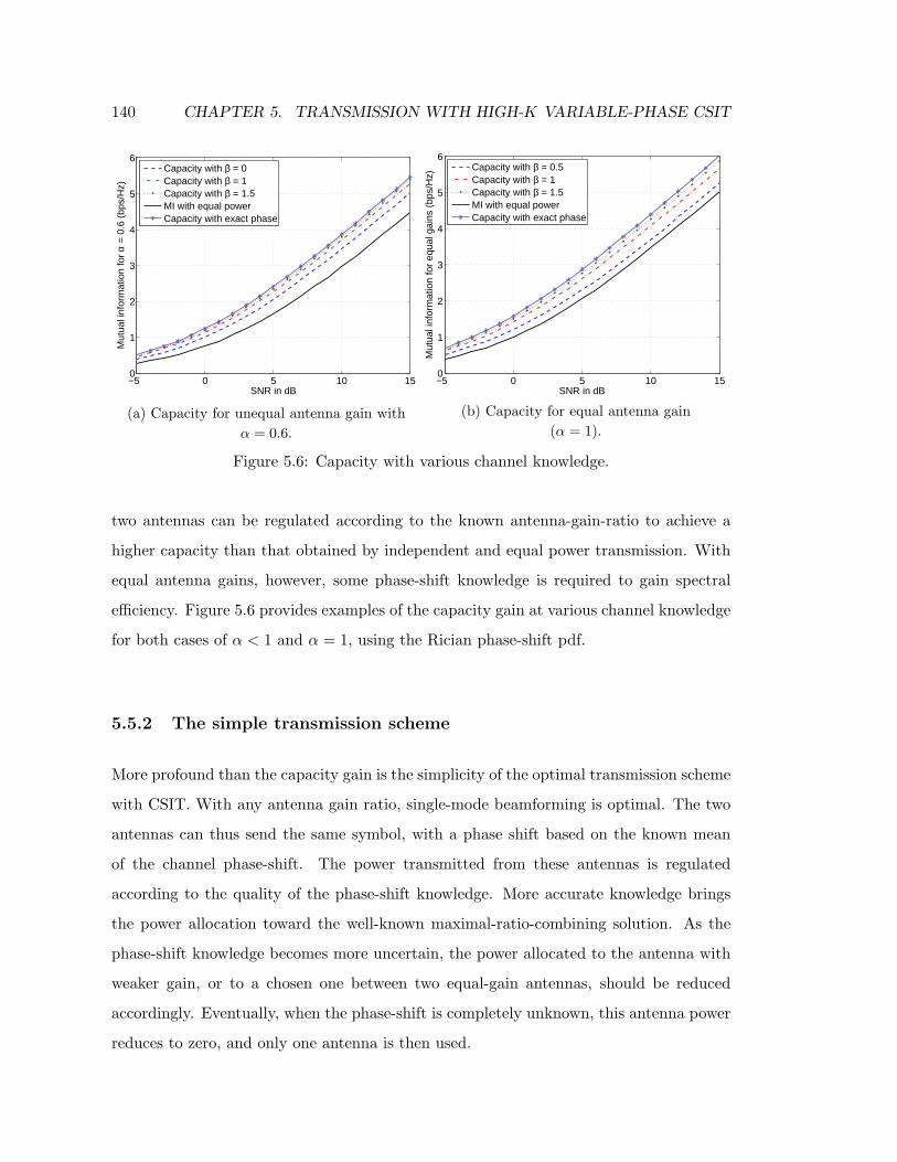
140 CHAPTER 5. TRANSMISSION WITH HIGH-K VARIABLE-PHASE CSIT
−5 0 5 10 150
1
2
3
4
5
6
SNR in dB
Mut
ual i
nfor
mat
ion
for α
= 0
.6 (
bps/
Hz)
Capacity with β = 0Capacity with β = 1Capacity with β = 1.5MI with equal powerCapacity with exact phase
(a) Capacity for unequal antenna gain with
α = 0.6.
−5 0 5 10 150
1
2
3
4
5
6
SNR in dB
Mut
ual i
nfor
mat
ion
for
equa
l gai
ns (
bps/
Hz)
Capacity with β = 0.5Capacity with β = 1Capacity with β = 1.5MI with equal powerCapacity with exact phase
(b) Capacity for equal antenna gain
(α = 1).
Figure 5.6: Capacity with various channel knowledge.
two antennas can be regulated according to the known antenna-gain-ratio to achieve a
higher capacity than that obtained by independent and equal power transmission. With
equal antenna gains, however, some phase-shift knowledge is required to gain spectral
efficiency. Figure 5.6 provides examples of the capacity gain at various channel knowledge
for both cases of α < 1 and α = 1, using the Rician phase-shift pdf.
5.5.2 The simple transmission scheme
More profound than the capacity gain is the simplicity of the optimal transmission scheme
with CSIT. With any antenna gain ratio, single-mode beamforming is optimal. The two
antennas can thus send the same symbol, with a phase shift based on the known mean
of the channel phase-shift. The power transmitted from these antennas is regulated
according to the quality of the phase-shift knowledge. More accurate knowledge brings
the power allocation toward the well-known maximal-ratio-combining solution. As the
phase-shift knowledge becomes more uncertain, the power allocated to the antenna with
weaker gain, or to a chosen one between two equal-gain antennas, should be reduced
accordingly. Eventually, when the phase-shift is completely unknown, this antenna power
reduces to zero, and only one antenna is then used.

5.6. CHAPTER SUMMARY 141
5.6 Chapter summary
This chapter has considered the 2×1 channel with partial CSIT consisting of the channel
amplitude and phase-shift pdf. The capacity-optimal transmission scheme is simple single-
mode beamforming on the mean of the channel phase shift. The two antennas then send
the same symbol, with per-antenna power adjusted according to the CSIT. If the antenna
gains are equal, the optimal scheme can also send different but correlated signals from the
two antennas. In all cases, when the channel phase-shift is known perfectly, the scheme
coincides with maximal-ratio-combining transmit beamforming. When the channel phase-
shift is completely unknown, the scheme reduces to single antenna transmission. This
partial CSIT thus helps simplify the transmission scheme significantly as single-mode
beamforming. At the same time, it provides a spectral efficiency gain of up to 1 bps/Hz
or an SNR advantage of up to 3dB for a MISO system with two transmit antennas.

Chapter 6
CONCLUSION
The main conclusion of this thesis is that intelligent use of transmit channel side informa-
tion in MIMO wireless is beneficial. The thesis has focused on studying two forms of side
information, namely dynamic CSIT and high-K variable-phase CSIT, and illustrated the
benefits by detailed capacity analysis and practical precoding designs. Results show that
even partial CSIT can help improve system performance in terms of the transmission rate
or reliability at a given transmit power. Naturally, the performance gain increases with
higher CSIT quality.
This chapter concludes the thesis. The chapter begins with a summary of the thesis
main results, follows by a brief overview of the deployment of precoding in emerging
wireless standards, and ends with a discussion of future research directions in exploiting
transmit channel information.
6.1 Thesis summary
This thesis has focused on exploiting channel side information at the transmitter (CSIT)
in a single-user MIMO wireless system. CSIT can increase MIMO capacity and enhance
system reliability. The time-varying nature of wireless channels, however, often degrades
the CSIT quality, posing challenges in system analysis and signal design.
The thesis contribution has been three fold: modeling dynamic CSIT, analyzing the
capacity gain and optimal input given a CSIT, and designing linear precoders to realize
142

6.1. THESIS SUMMARY 143
the gain. The dynamic CSIT model takes into account the channel temporal variation
by using an initial, potentially outdated channel measurement and the channel statistics,
including the mean, covariance, and temporal correlation [18]. The model consists of a
channel estimate and its error covariance, which function as an effective channel mean
and an effective channel covariance, respectively. Both parameters are functions of the
channel temporal correlation factor ρ, which indicates the CSIT quality. Depending on
this quality, the model covers smoothly from perfect (ρ = 1) to statistical (ρ = 0) CSIT
[18, 19] (Chapter 2).
Second, the thesis analyzes the capacity gain and the optimal input with dynamic
CSIT asymptotically at low and high SNRs [20], and develops a convex optimization
program to find the capacity non-asymptotically [22]. The program helps to assess the
tightness of a simple capacity lower-bound, based on the Jensen optimal input. Results
differ with SNR and the relative number of antennas. At low SNRs, the capacity lower-
bound is tight for all systems. The capacity gain here is multiplicative, and the optimal
input is typically simple single-mode beamforming. At high SNRs, for systems with equal
or fewer transmit than receive antennas, the capacity bound is also tight, but the capacity
gain diminishes to zero due to equi-power optimal input. For other systems, the bound
becomes loose at high SNRs, but the capacity gain is additive and the optimal input may
drop modes, if the channel mean or transmit antenna correlation is strong (Chapter 3).
Third, linear precoders exploiting CSIT are designed, using convex analysis and matrix
algebra. Optimal from an information theoretic viewpoint, a linear precoder functions as
a multi-mode beamformer. It decouples the transmit signal into orthogonal eigen-beams
and assigns higher power to the directions where the channel is strong, but reduced or
no power to the weak. For dynamic CSIT, an optimal precoder is constructed using a
dynamic water-filling process [23]. The design obtains a range of significant and robust
precoding gains, depending on the CSIT quality [18] (Chapter 4). Another precoder is de-
signed for high-K variable-phase CSIT, which reduces to simple single-mode beamforming
with variable antenna power allocation, depending on the channel phase-shift information
[24] (Chapter 5).
For dynamic CSIT, a common observation emerging from the capacity and precoding

144 CHAPTER 6. CONCLUSION
results is that, the performance gain becomes sensitive to the CSIT quality only at rela-
tively high quality, approximately ρ ≥ 0.6. Otherwise, it is similar to the gain obtained
from statistical CSIT at ρ = 0. This observation suggests that, in dynamic CSIT, the
initial channel measurement is useful only when its correlation with the current channel
is relatively strong; otherwise, using the channel statistics alone achieves most of the
performance gain.
6.2 Precoding deployment in wireless standards
Precoding has been successfully incorporated in the IEEE 802.16e standard for broadband
wireless metropolitan networks [3]. The standard supports both closed- and open-loop
precoding for the downlink. In the closed-loop method, the precoder is based on either
an initial channel measurement or the channel statistics, corresponding to CSIT quality
ρ = 1 or ρ = 0, respectively. The user-unit measures the channel and the fading rate,
using the forward-link preambles or pilots. Based on the channel measurement, it picks a
short-term precoding matrix from a codebook of unitary precoders, containing the beam
directions. The fading rate is used to calculate a time-to-live parameter, which is fed
back to the basestation along with the short-term precoding index. The basestation uses
this short-term precoding matrix until the time-to-live expires. Thereafter, it precodes
using channel statistics information, which is updated at a much slower rate and is always
valid. In the open-loop method, a subset of users is scheduled to transmit a sounding
signal. The base station then estimates the channels for these users and determines the
CSIT based on reciprocity after transmit-receive RF calibration.
MIMO is entering the IEEE 802.11n standard for wireless local area networks (WLANs).
The standard supports both space-time coding and spatial multiplexing. The current pre-
coding proposals use an open-loop method, relying on the reciprocity principle that the
best beam on reception must be the best beam for transmission. The access point thus
uses pre-formed beams for receiving and transmitting, and records the beam(s) with
the best signal strength on reception for each user, then uses the same beam(s) during
transmission.

6.3. FUTURE DIRECTIONS 145
The 3GPP standard uses a closed-loop beamforming technique, based on feedback of
the channel phase and amplitude information. Precoding is under discussion in High-
Speed Downlink Packet Access (HSDPA) for mobile communication. Channel-sounding
techniques appear to be preferred.
6.3 Future directions
Exploiting CSIT is a current research area with still many open problems in both single-
and multi-user domains. In single-user, for examples, an analytical solution for the op-
timal precoder with statistical CSIT (both mean and covariance) under the capacity
criterion remains unsolved. Precoding with a more general channel covariance structure,
such as a non-Kronecker model, has hardly been studied. Extension to frequency selective
channels increases the complexity in acquiring and modeling partial CSIT and requires
efficient precoding techniques [82]. Codebook design and its application in compressing
channel information efficiently for closed-loop systems is also a rich research area [38, 40].
Another practical question is the tradeoff between overheads in CSIT acquisition and
performance gains from the CSIT.
In multi-user communication, exploiting partial CSIT is an important open problem.
Recent results have established the capacity regions for the Gaussian multiple access and
broadcast channels [46, 83]. Dirty-paper coding [84], for example, is a capacity-optimal
precoding scheme for the broadcast channel. These results, however, require full channel
information at all transmitters and receivers, which is quite impractical in wireless, where
obtaining CSIT usually demands substantial resources. Initial research has shown that
the loss of degrees of freedom due to the lack of CSIT reduces the capacity region of
an isotropic vector broadcast-channel to that of a scalar one [85]. Imperfect CSIT also
severely reduces the growth of the sum-rate broadcast capacity at high SNRs [86]. Further
research are required to characterize multi-user partial CSIT and their impacts on the
channel capacity, and to design signal processing schemes given the CSIT.
Opportunistic scheduling is a scheme exploiting multi-user diversity by serving the
users with the best channels each time. It achieves an optimal throughput growth-rate

146 CHAPTER 6. CONCLUSION
with a large number of users [87, 88]. This growth, however, assumes arbitrary delay
and accurate instantaneous CSIT, both are unrealistic in practical wireless systems. A
study of hard delay constraints has revealed drop in system throughput for an increasing
number of users [89]. Erroneous CSIT, likewise, will reduce the system throughput.
Understanding this effect requires further research.

Appendix A
Derivations and Proofs
A.1 K-factor threshold for mode-dropping at all SNRs
This section provides the derivation for (3.20). In problem (3.19), replacing λ2 as a
function of λ1, noting that the optimal λ1 ≥ λ2, the problem becomes equivalent to
maxλ1
g(λ1) = Ehj
log det
IM + λ1γ
M∑
j=1
hjh∗j +
1 − Mλ1
N − Mγ
N∑
j=M+1
hjh∗j
subject to1
N≤ λ1 ≤ 1
M,
where hj =(
βej + hj
)
. Since problem (3.19) is convex, this problem is convex. Thus, to
have the optimal λ?1 = 1/M , it is sufficient and necessary that dg(λ1)
dλ1
∣
∣
∣
λ1=1/M≥ 0, which
translates to
0 ≤ Ehj
tr
IM +γ
M
M∑
j=1
hjh∗i
−1
γ
M∑
j=1
hjh∗i −
γM
N − M
N∑
j=M+1
hjh∗j
(a)= M2 − ME
hj
tr
IM +γ
M
M∑
j=1
hjh∗i
−1
IM +γ
N − M
N∑
j=M+1
hjh∗j
,
where (a) follows from adding and subtracting MIM in the second parenthetic factor
inside the trace expression, and hj and hj are independent. Due to this independence,
147

148 APPENDIX A. DERIVATIONS AND PROOFS
and noting that hj ∼ N(
0, (1 − β2)IM
)
, the above inequality leads to
M ≥ tr
Ehj
IM +γ
M
M∑
j=1
hjh∗i
−1
Ehj
IM +γ
N − M
N∑
j=M+1
hjh∗j
= tr
Ehj
IM +γ
M
M∑
j=1
hjh∗i
−1
[
1 + γ(
1 − β2)]
.
This expression results in (3.20).
A.2 Rt condition-number threshold for mode-dropping at
all SNRs
This section provides the derivation for (3.25). In problem (3.24), replacing λ1 as a
function of λ2 and noting that λ1 ≥ λ2, the problem becomes equivalent to
maxλ2
f(λ2) = Ehi
log det
IM + γ1 − (N − L)λ2
Lξ1
L∑
i=1
hih∗i + γλ2ξ2
N∑
j=L+1
hjh∗j
subject to 0 ≤ λ2 ≤ 1
N,
where hi ∼ N (0, IM ). The condition for the optimal λ?2 = 0 is ∂f
∂λ2
∣
∣
∣
λ2=0≤ 0, which
translates to
0 ≥ Ehi
tr
IM +γξ1
L
L∑
j=1
hih∗i
−1
γξ2
N∑
j=L+1
hjh∗j − γξ1
N − L
L
L∑
i=1
hih∗i
(a)= tr
Ehi
IM +γξ1
L
L∑
j=1
hih∗i
−1
γξ2IM − γξ1
L
L∑
j=1
hih∗i
(N − L)
= tr
Ehi
IM +γξ1
L
L∑
j=1
hih∗i
−1
(γξ2 + 1)IM −
IM +γξ1
L
L∑
j=1
hih∗i
× (N − L)
=
tr
Ehi
IM +γξ1
L
L∑
j=1
hih∗i
−1
(γξ2 + 1)
− M
(N − L) ,

A.3. SOLVING A QUADRATIC MATRIX EQUATION 149
where (a) follows from the mutually exclusive, independent sums and E[
∑Nj=L+1 hjh
∗j
]
=
(N − L)IM . The above inequality leads to (3.25).
A.3 Solving a quadratic matrix equation
This section solves the quadratic matrix equation (4.23). Rewrite this equation by mul-
tiplying left and right with W as
νWR−2t W − MW − H∗
mHm = 0 . (A.1)
This is a matrix quadratic equation in W, which can be solved similarly to a scalar
equation. Recall that the scalar quadratic equation
ax2 + bx + c = 0
has the solution as
x =1
2a
(
−b ±√
∆)
where ∆ = b2 − 4ac. In the matrix equation (A.1),
a ∼ νR−2t
b ∼ −MIN
c ∼ −H∗mHm.
Form the matrix equivalence of ∆ as in (4.25)
Ψ = M2IN + 4νR−1t H∗
mHmR−1t ,
in which a is split around c to ensure symmetry. The solutions then follow as
W =1
2νRt
(
MIN ± Ψ1
2
)
Rt ,

150 APPENDIX A. DERIVATIONS AND PROOFS
in which a−1 is again split on two sides. The positive semidefinite value of W is chosen
as in (4.24).
A quick check to verify the answer can be carried out by plugging the solutions into
(A.1) as
νWR−2t W − MW − H∗
mHm
=1
4νRt
(
MIN ± Ψ1
2
)2Rt −
M
2νRt
(
MIN ± Ψ1
2
)
Rt − H∗mHm
=1
4νRt
(
M2IN ± 2MΨ1
2 + Ψ)
Rt −M
2νRt
(
MIN ± Ψ1
2
)
Rt − H∗mHm
= −M2
4νR2
t +1
4νRtΨRt − H∗
mHm
= −M2
4νR2
t +1
4νRt
(
M2IN + 4νR−1t H∗
mHmR−1t
)
Rt − H∗mHm
= 0.
A.4 Deriving the bounds on ν in the outer algorithm
To derive the bounds in (4.30), apply Weyl’s theorem [72] λ1(A) + λk(B) ≤ λk(A + B) ≤λN (A) + λk(B) to the left-hand-side expression in (4.29). The following bounds on this
expression, with k modes dropped (1 ≤ k ≤ N − 1), are obtained:
fupper=M(N − k)
2ν+ (N − k)
√
M2 + 4νλN
2ν−
N∑
i=k+1
1
λi(Rt)
flower=M(N − k)
2ν+ (N − k)
√M2 + 4νλ1
2ν−
N∑
i=k+1
1
λi(Rt).
Equating each bound to η0 results in a quadratic equation, from which the corresponding
value for ν in (4.30) is derived.
A.5 Solving the trace relaxation problem
To solve (4.37), again form the Lagrangian and differentiate with respect to W to obtain
−W−1H∗mHmW−1 − MW−1 + νR−1
t Λ−1A R−1
t = 0 ,

A.5. SOLVING THE TRACE RELAXATION PROBLEM 151
where ν is the Lagrange multiplier associated with the equality constraint. Let G be the
Hermitian matrix such that RtΛARt = G2, then the above quadratic matrix equation
has the solution
W =1
2νG
(
MIN + Ψ1
2
)
G ,
where
Ψ = M2IN + 4νG−1H∗mHmG−1 .
Now B can be written as
B =4
ρ
[
1
2νR−1
t G(
MIN + Ψ(ν)1
2
)
GR−1t − R−1
t
]
,
and the product Λ−1A B becomes
Λ−1A B =
4
ρ
(
M
2νIN +
1
2νΛ−1
A R−1t GΨ
1
2 GR−1t − Λ−1
A R−1t
)
.
The Lagrange multiplier ν must satisfy the equality constraint in (4.37), or equiv-
alently, tr(
Λ−1A B
)
= 1, while ensuring B < 0. Similar to the orthogonal STBC case,
ν is solved in two steps. First, assume that B is full-rank and solve the equation
tr(
Λ−1A B
)
= 1. If the resulting B is not PSD, then drop the weakest eigen-mode of
B and resolve for ν, using the equation
N∑
i=k+1
λi
(
Λ−1A B
)
= 1 ,
where k is the number of dropped modes, and keep dropping modes until B is PSD. In
this case, the eigenvalues of Λ−1A B cannot be written explicitly as functions of ν to obtain
an equation similar to (4.27). Nevertheless, since the eigenvalue sum is monotonic in ν,
similarly, ν can be found by performing an one-dimensional binary search in each step.
The bounds on ν for the equation with k modes dropped (0 ≤ k ≤ N − 1) are given by
νbound =α
β2+
M
β, (A.2)

152 APPENDIX A. DERIVATIONS AND PROOFS
where for the upper bound
α = λmax
(
G−1H∗mHmG−1
)
β = λmin
(
Λ−1A R−1
t
)
+ρ
4(N − k),
and for the lower bound
α = λmin
(
G−1H∗mHmG−1
)
β = λmax
(
Λ−1A R−1
t
)
+ρ
4(N − k).
To derive the upper bound, use the inequality∑N
k+1 λi(Λ−1A B) ≤ (N −k)λmax(Λ
−1A B)
and further obtain an upper bound on λmax(Λ−1A B) as
λmax(Λ−1A B) ≤ 4
ρ
[
M
2ν+
1
2νλmax
(
Λ−1A R−1
t GΨ1
2 GR−1t
)
− λmin
(
Λ−1A R−1
t
)
]
,
invoking the inequality λmax(A + B) ≤ λmax(A) + λmax(B) for Hermitian matrices [73].
The following chain holds:
λmax
(
Λ−1A R−1
t GΨ1
2 GR−1t
)
(a)= λmax
(
GR−1t Λ−1
A R−1t GΨ
1
2
)
(b)
≤ λmax
(
GR−1t Λ−1
A R−1t G
)
λmax
(
Ψ1
2
)
(c)= λmax
(
Λ−1/2A R−1
t G2R−1t Λ
−1/2A
)
λmax
(
Ψ1
2
)
(d)= λmax
(
Ψ1
2
)
(e)=
√
M2 + 4νλmax (G−1H∗mHmG−1) ,
where (a) and (c) follow from λ(AB) = λ(BA) [72], (b) follows from λmax(AB) ≤λmax(A)λmax(B) for Hermitian matrices [73], (d) follows from the definition for G, and
(e) follows from λ(I+A) = 1+λ(A). The upper bound on ν can then be found by solving
M
2ν+
1
2ν
√
M2 + 4να − β = 0
with α and β specified above. The lower bound is derived similarly.

A.6. OPTIMAL PRECODER WITH MEAN CSIT AND NON-IDENTITY A 153
A.6 Optimal precoder with mean CSIT and non-identity A
This section provides the derivation for the optimal precoder with mean CSIT given a
non-identity A in (4.53) and (4.54). From problem (4.52), form the Lagrangian as
L (ν, λi(B)) =∑
i
(
1 +γ
4λi(B)
)−1λm,i−M
∑
i
log(
1 +γ
4λi(B)
)
−ν
(
∑
i
ξiλi(B) − 1
)
.
where ν is the Lagrange multiplier associated with the equality constraint. Take the
derivative of L (ν, λi(B)) with respect to λi(B) and set it to zero to get
γλm,i
4(
1 + γ4λi(B)
)2 − Mγ
4(
1 + γ4λi(B)
) − νξi = 0
Let z = 1 + γ4λi(B), the above equation is equivalent to
4νξiz2 + Mγz − γλm,i = 0 ,
which leads to
z =1
8νξi
(
Mγ ±√
M2γ2 + 16νξiγλm,i
)
.
Replacing this result into λi(B) = 4(z − 1)/γ, noting that λi(B) ≥ 0 and that ξi =
1/λi(A), expression (4.53) then follows.
To find the Lagrange multiplier ν, solve the equality constraint, which now becomes
N∑
i=1
[
1
2ν
(
M +
√
M2 + 16νλm,i
γλi(A)
)
− 4
γλi(A)
]
+
= 1 .
The upper- and lower-bounds on the solution for ν can be established by replacing
λm,i/λi(A) with its largest and smallest values, λN and λ1, respectively. With k dropped
modes, the equation for the upper bound becomes
(N − k)
2ν
M +
√
M2 + 16νλN
γ
−N
∑
i=k+1
4
γλi(A)= 1 .

154 APPENDIX A. DERIVATIONS AND PROOFS
With ζk defined in (4.55), the above equation can be rewritten as
√
M2 + 16νλN
γ= 2ζkν − M .
Solving this equation leads to the upper bound for ν in (4.54). The lower bound is derived
similarly.
A.7 Optimal beam directions with transmit covariance CSIT
This sections proves (4.61) as the optimal beam directions for problem (4.60). Consider
the following more constrained problem
max EHw
[
f
(
I + aρHwR1
2
t FQF∗R1
2
t H∗w
)]
(A.3)
subject to tr (FF∗) = 1
tr
(
R1
2
t FQF∗R1
2
t
)
= ξ ,
where ξ is equal to that resulted from the optimal solution of (4.60). Due to the setup,
the two problems are equivalent: the second formulation is more constrained and hence
has a smaller or equal optimal value compared to the first formulation; and the choice of
ξ makes the two optimal values the same.
Now consider the second problem (A.3) by itself, the chosen ξ must be the largest
feasible value. The reason is that, if a feasible ξ2 is larger than ξ1, then the objective
function in the problem with ξ2 can be chosen to be larger than that with ξ1, hence
causing contradiction. Based on the inequality Rtr(A1 · · ·Am) ≤ ∑
i σi(A1) · · ·σi(Am)
for complex matrices [73], without affecting the singular values of F and hence the power
constraint, the value ξ is largest when the right and left singular vectors of F are the same
as the eigenvectors of Q and Rt, respectively. In other words, the optimal conditions for
the precoder singular vectors are
UF = Ut
VF = UQ ,

A.8. OPTIMAL PHASE-SHIFT WITH HIGH-K VARIABLE-PHASE CSIT 155
which proves (4.61), and concurrently (4.57).
A.8 Optimal phase-shift with high-K variable-phase CSIT
This section analyzes the two choices for the optimal signal phase-shift in (5.10). With
ψ = −φ0, the average mutual information (5.8) becomes
I|ψ=−φ0= 2
∫ π
0log (p + γαρ cos φ) f(φ)dφ .
For ψ = π − φ0, a similar expression is obtained but with the plus sign replaced by a
minus sign. The difference between I at the two candidates for φ? is
∆I = I|ψ=−φ0− I|ψ=π−φ0
= 2
∫ π
0log
(
p + γαρ cos φ
p − γαρ cos φ
)
f(φ) dφ .
The logarithmic expression is anti-symmetric around π/2, therefore the above difference
can be rewritten as
∆I = 2
∫ π/2
0log
(
2p
p − γαρ cos φ− 1
)
[
f(φ) − f(
φ +π
2
)]
dφ .
Since the logarithmic expression in the above integral is non-negative within the integral
range, if f(φ) − f(
φ + π2
)
has only one sign within this range, then the sign of ∆I can
be simply determined without having to evaluate the integral explicitly. Specifically, if
the translated phase-shift pdf f(φ) is monotonous within the range 0 ≤ φ ≤ π, then the
choice between φ = 0 and φ = π that makes f(φ) larger determines the optimal ψ? to be
−φ0 or π − φ0, respectively.

Appendix B
Simulation Parameters
B.1 Channel parameter normalization
This section discusses the channel normalization used in simulations. Consider a frequency-
flat quasi-static block fading MIMO wireless channel with N transmit and M receive
antennas. For simulations, the channel is normalized for a constant average power gain of
MN , such that E[tr(H∗H)] = MN . The transmit signal power is assumed to have been
adjusted accordingly. The normalization ensures a fair performance comparison between
systems operating on channels with different mean or covariance matrices and, therefore,
allows an objective gain measure (otherwise, a stronger channel power-gain will likely
result in a better precoding or capacity gain).
With normalization, the channel mean (2.19) and covariance (2.16) can be written as
Hm =
√
K
K + 1Hm (B.1)
R0 =1
K + 1R0 ,
where Hm and R0 are the normalized channel mean and covariance, such that
||Hm||2F = MN
tr(R0) = MN .
156

B.2. PARAMETERS FOR CAPACITY OPTIMIZATION 157
For the Kronecker antenna correlation model (2.17), the normalized channel covariance
can be written as
R0 = RTt,0 ⊗ Rr,0 ,
where
tr(Rt,0) = N
tr(Rr,0) = M .
When transmit antenna correlation alone exists, it can be written as
Rt =1
K + 1Rt,0 ,
while Rr = I. Consequently, normalized CSIT parameters are specified.
B.2 Parameters for capacity optimization
This section lists the CSIT parameters for capacity optimization in Sections 3.4.2 and
3.5. All simulated channels have 4 transmit and either 2 or 4 receive antennas. The
normalized transmit covariance matrix is
Rt,0 =
0.8758 −0.0993 − 0.0877i −0.6648 − 0.0087i 0.5256 − 0.4355i
−0.0993 + 0.0877i 0.9318 0.0926 + 0.3776i −0.5061 − 0.3478i
−0.6648 + 0.0087i 0.0926 − 0.3776i 1.0544 −0.6219 + 0.5966i
0.5256 + 0.4355i −0.5061 + 0.3478i −0.6219 − 0.5966i 1.1379
.
This matrix has the eigenvalues as [2.717, 0.997, 0.237, 0.049] and a condition number of
55.5, representing strong antenna correlation. The normalized mean for the 4×2 channel
is
Hm =√
10
0.0749 − 0.1438i 0.0208 + 0.3040i −0.3356 + 0.0489i 0.2573 − 0.0792i
0.0173 − 0.2796i −0.2336 − 0.2586i 0.3157 + 0.4079i 0.1183 + 0.1158i
.

158 APPENDIX B. SIMULATION PARAMETERS
The normalized mean for the 4 × 4 channel is
Hm =√
10
0.2976 + 0.1177i 0.1423 + 0.4518i −0.0190 + 0.1650i −0.0029 + 0.0634i
−0.1688 − 0.0012i −0.0609 − 0.1267i 0.2156 − 0.5733i 0.2214 + 0.2942i
0.0018 − 0.0670i 0.1164 + 0.0251i 0.5599 + 0.2400i 0.0136 − 0.0666i
−0.1898 + 0.3095i 0.1620 − 0.1958i 0.1272 + 0.0531i −0.2684 − 0.0323i
.
The simulated channels have K = 0.1.
The parameters used in the convex optimization programs are
Maximum number of iterations MAXITER = 10
Maximum number of line searches each step MAXLINES = 50
Initial barrier multiplying factor barr t = 100
Barrier method update factor µ = 100
Tolerance (∆xTnt∇2f(x)∆xnt ≤ ε) ε = 10−5
Number of channel samples in Monte-Carlo simulations NSAMPLE = 20000 .
B.3 Parameters for precoding with dynamic CSIT
The channel parameters used in the precoding simulations in Section 4.3.3 are as follows.
For the 2 × 1 channel
Hm =√
10[
+0.3805 + 0.1069i −0.1845 − 0.0985i]
,
Rt,0 =
1.1843 −0.7537 + 0.5638i
−0.7537 − 0.5638i 0.8157
.
For the 4 × 1 channel
Hm =√
10[
0.2727 − 0.1675i −0.0577 + 0.1771i 0.1421 + 0.2523i 0.3283 − 0.2670i]
,
Rt,0 =
0.8611 0.2582 − 0.6041i 0.2458 − 0.1377i 0.1637 + 0.0991i
0.2582 + 0.6041i 1.0311 0.5159 + 0.0262i −0.0935 − 0.0804i
0.2458 + 0.1377i 0.5159 − 0.0262i 0.7158 −0.5048 − 0.2518i
0.1637 − 0.0991i −0.0935 + 0.0804i −0.5048 + 0.2518i 1.3921
.

B.4. PARAMETERS FOR PRECODING COMPARISON 159
The simulated channels have K = 0.1, except for Figure 4.6, in which K varies.
B.4 Parameters for precoding comparison
The 4 × 2 channel parameters used in the precoding comparison in Section 4.6 are as
follows. The transmit covariance matrix is
Rt,0 =
0.8758 −0.0993 − 0.0877i −0.6648 − 0.0087i 0.5256 − 0.4355i
−0.0993 + 0.0877i 0.9318 0.0926 + 0.3776i −0.5061 − 0.3478i
−0.6648 + 0.0087i 0.0926 − 0.3776i 1.0544 −0.6219 + 0.5966i
0.5256 + 0.4355i −0.5061 + 0.3478i −0.6219 − 0.5966i 1.1379
.
The channel mean matrix used in dynamic CSIT is
Hm =√
10
0.0749 − 0.1438i 0.0208 + 0.3040i −0.3356 + 0.0489i 0.2573 − 0.0792i
0.0173 − 0.2796i −0.2336 − 0.2586i 0.3157 + 0.4079i 0.1183 + 0.1158i
.
Again, the simulated channels have K = 0.1, except for Figure 4.11, in which K varies.

Notation
Acronyms
BER Bit error rate.
CSIR Channel side information at the receiver.
CSIT Channel side information at the transmitter.
EVD Eigenvalue decomposition.
FDD Frequency-division duplex.
IEEE Institute of Electrical and Electronic Engineers.
MIMO Multiple-input multiple-output.
MISO Multiple-input single-output.
MMSE Minimum mean squared-error.
MSE Mean squared-error.
PEP Pair-wise error probability.
QSTBC Quasi-orthogonal STBC.
RF Radio frequency.
SNR Signal to noise ratio.
ST Space-Time.
STBC Space-time block code.
SVD Singular value decomposition.
TDD Time-division duplex.
160

NOTATION 161
Operations
E[.] Expected value.
⊗ Kronecker product.
Pr(.) Probability.
exp(.) Exponential.
Re The real part.
Im The imaginary part.
¿ Significantly less than.
(.)? Optimal value.
(x)+ max (x, 0), where x is real.
Vectors and Matrices
X Matrix X (bold-face capital letter).
x Vector x (bold-face lower-case letter).
XT Transpose of X.
X∗ Conjugate transpose of X.
det(X) Determinant of X.
tr(X) Trace of X.
||X||F Frobenius norm of X.
λi(X) Eigenvalues of a Hermitian matrix X.
σi(X) Singular values of X.
ΛX The diagonal matrix of the eigenvalues of X.
ΣX The diagonal matrix of the singular values of X.
UX ,VX The eigen- or singular-vector matrix of X.
X < 0 X is positive semi-definite.
vec(X) Vectorize X by concatenating the columns of X.
I An identity matrix.
N (Hm,R0) Gaussian distribution with mean Hm and covariance R0.

162 NOTATION
Symbols
C Channel ergodic capacity.
I Mutual information.
N The number of transmit antennas.
M The number of receive antennas.
Kt The rank of the transmit covariance matrix.
h A scalar wireless channel.
H A MIMO flat-fading channel.
H0 A channel measurement (sample) at time 0.
Hw A random channel with i.i.d zero-mean unit-variance
circular complex Gaussian elements.
Hm The channel mean.
R0,R The channel covariance and auto-covariance.
Rt Transmit covariance, also called transmit antenna correlation.
Rr Receive covariance, also called receive antenna correlation.
H A channel estimate.
E Estimation error.
Re The error or effective covariance.
ρ The channel temporal correlation function.
K The Rician K factor
Tc The channel coherence time.
Bc The channel coherence bandwidth.
t Continuous time.
∆t Delay.
n, m Discrete time or delay.
F The precoding matrix.
D The diagonal matrix of the singular-values of F.
pi Power loading on beam i.
C A codeword.
Q The codeword covariance matrix or input covariance.
A The codeword difference product matrix.
γ The signal to noise ratio.
ν The Lagrange multiplier.
δ The Dirac delta function.
φ, ψ Phase or phase-shift.
Pe System error probability.
X,X The transmit signal.
Y,Y The receive signal.

Bibliography
[1] S. Nanda, R. Walton, J. Ketchum, M. Wallace, and S. Howard, “A high-performance
MIMO OFDM wireless LAN,” IEEE Communications Magazine, vol. 43, no. 2, pp.
101–109, Feb. 2005.
[2] I. S. 802.11n, “Part 11: Wireless LAN medium access control (MAC) and physical
layer (PHY) specifications - High throughput,” Working IEEE Standards, 2006.
[3] I. S. 802.16e, “Part 16: Air interface for fixed and mobile broadband wireless access
systems,” IEEE Standards, Oct 2005.
[4] E. S. Brown, “The selling of cell phone
TV,” Technology Review, Nov. 2004. [Online]. Available:
http://www.technologyreview.com/read article.aspx?id=13901&ch=infotech
[5] L. Yang and G. Giannakis, “Ultra-wideband communications: An idea whose time
has come,” IEEE Signal Processing Magazine, vol. 21, no. 6, pp. 26–54, Nov. 2004.
[6] I. Telatar, “Capacity of multi-antenna Gaussian channels,” Bell Laboratories
Technical Memorandum, http://mars.bell-labs.com/papers/proof/, Oct. 1995.
[Online]. Available: http://mars.bell-labs.com/papers/proof/
[7] A. Paulraj, R. Nabar, and D. Gore, Introduction to Space-Time Wireless Communi-
cations. Cambridge, UK: Cambridge University Press, 2003.
[8] I. S. 802.20, “Part 20: Mobile broadband wireless access (MBWA),” Working IEEE
Standards, 2006.
[9] A. Hottinen, O. Tirkkonen, and R. Wichman, Multi-antenna transceiver techniques
for 3G and beyond. Wiley & Sons, Inc., 2003.
[10] A. Paulraj and C. Papadias, “Space-time processing for wireless communications,”
IEEE Signal Processing Magazine, vol. 14, no. 6, pp. 49–83, Nov. 1997.
163

164 BIBLIOGRAPHY
[11] G. Caire and S. S. Shamai, “On the capacity of some channels with channel state
information,” IEEE Trans. on Info. Theory, vol. 45, no. 6, pp. 2007–2019, Sep. 1999.
[12] C. Shannon, “Channels with side information at the transmitter,” IBM J. of Research
and Devel., vol. 2, no. 4, pp. 289–293, Oct. 1958.
[13] M. Skoglund and G. Jongren, “On the capacity of a multiple-antenna communication
link with channel side information,” IEEE J. on Selected Areas in Comm., vol. 21,
no. 3, pp. 395–405, Apr. 2003.
[14] W. Jakes, Microwave Mobile Communications. IEEE Press, 1994.
[15] T. Rappaport, Wireless Communications: Principles and Practice. Prentice Hall
PTR, 1996.
[16] A. Goldsmith and P. Varaiya, “Capacity of fading channels with channel side infor-
mation,” IEEE Trans. Info. Theory, vol. 43, no. 6, pp. 1986–1992, Nov. 1997.
[17] V. Tarokh, H. Jafarkhani, and R. Calderbank, “Space-time block codes from or-
thogonal designs,” IEEE Trans. on Info. Theory, vol. 45, no. 5, pp. 1456–1467, July
1999.
[18] M. Vu and A. Paulraj, “A robust transmit CSI framework with applications in MIMO
wireless precoding,” Proc. 39th Asilomar Conf. Sig., Sys. and Comp., Nov. 2005.
[19] ——, MIMO Wireless Communications. Cambridge University Press, 2006, ch.
Precoding design.
[20] ——, “Characterizing the capacity for MIMO wireless channels with non-zero mean
and transmit covariance,” Proc. Forty-Third Allerton Conf. on Comm., Control, and
Comp., Sep. 2005.
[21] ——, “Some asymptotic capacity results for MIMO wireless with and without channel
knowledge at the transmitter,” Proc. 37th Asilomar Conf. Sig., Sys. and Comp.,
vol. 1, pp. 258–262, Nov. 2003.
[22] ——, “Capacity optimization for Rician correlated MIMO wireless channels,” Proc.
39th Asilomar Conf. Sig., Sys. and Comp., Nov. 2005.
[23] ——, “Optimal linear precoders for MIMO wireless correlated channels with nonzero
mean in space–time coded systems,” IEEE Trans. on Signal Processing, vol. 54, no. 6,
pp. 2318–2332, June 2006.

BIBLIOGRAPHY 165
[24] ——, “Optimum space-time transmission for a high K factor wireless channel with
partial channel knowledge,” Wiley Journal on Wireless Comm. and Mobile Comput-
ing, vol. 4, pp. 807–816, Nov. 2004.
[25] J. Proakis, Digital Communications. McGraw-Hill, 1989.
[26] H. Hasemi, “The indoor radio propagation channel,” Proceedings of the IEEE, vol. 8,
no. 7, pp. 943–968, July 1993.
[27] A. Papoulis, Probability, Random Variables, and Stochastic Processes. McGraw-Hill
Inc., 1991.
[28] S. Rice, “Statistical properties of a sine wave plus random noise,” Bell Systems
Technical Journal, vol. 27, pp. 109–157, Jan 1948.
[29] D. Shiu, G. Foschini, M. Gans, and J. Kahn, “Fading correlation and its effect on the
capacity of multielement antenna systems,” IEEE Trans. on Comm., vol. 48, no. 3,
pp. 502–513, Mar. 2000.
[30] A. Graham, Kronecker Products and Matrix Calculus with Application. Ellis Hor-
wood Ltd., 1981.
[31] K. Yu, M. Bengtsson, B. Ottersten, D. McNamara, P. Karlsson, and M. Beach,
“Second order statistics of NLOS indoor MIMO channels based on 5.2 GHz mea-
surements,” Proc. IEEE Global Telecomm. Conf., vol. 1, pp. 25–29, Nov. 2001.
[32] J. Kermoal, L. Schumacher, K. Pedersen, P. Mogensen, and F. Frederiksen, “A
stochastic MIMO radio channel model with experimental validation,” IEEE J. on
Selected Areas in Comm., vol. 20, no. 6, pp. 1211–1226, Aug. 2002.
[33] D. Bliss, A. Chan, and N. Chang, “MIMO wireless communication channel phe-
nomenology,” IEEE Trans. on Antennas and Propagation, vol. 52, no. 8, pp. 2073–
2082, Aug. 2004.
[34] A. Sayeed, “Deconstructing multiantenna fading channels,” IEEE Trans. on Signal
Proc., vol. 50, no. 10, pp. 2563–2579, Oct. 2002.
[35] W. Weichselberger, M. Herdin, H. Ozcelik, and E. Bonek, “A stochastic MIMO
channel model with joint correlation of both link ends,” IEEE Trans. on Wireless
Comm., vol. 5, no. 1, pp. 90–100, Jan. 2006.
[36] D. Baum, D. Gore, R. Nabar, S. Panchanathan, K. Hari, V. Erceg, and A. Paulraj,
“Measurement and characterization of broadband MIMO fixed wireless channels at
2.5ghz,” Proc. Int’l Conf. Per. Wireless Comm., pp. 203–206, Dec. 2000.

166 BIBLIOGRAPHY
[37] A. Bourdoux, B. Come, and N. Khaled, “Non-reciprocal transceivers in
OFDM/SDMA systems: Impact and mitigation,” Proc. Radio and Wireless Conf.,
pp. 183–186, Aug. 2003.
[38] B. Hochwald, T. Marzetta, T. Richardson, W. Sweldens, and R. Urbanke, “Sys-
tematic design of unitary space-time constellations,” IEEE Trans. Info. Theory, pp.
1962–1973, Sep. 2000.
[39] D. Love and R. Heath, Jr., “Limited feedback unitary precoding for spatial multi-
plexing,” IEEE Trans. Info. Theory, vol. 51, no. 8, pp. 2967–2976, Aug. 2005.
[40] ——, “Limited feedback unitary precoding for orthogonal space-time block codes,”
IEEE Trans. Signal Processing, vol. 53, no. 1, pp. 64–73, Jan. 2005.
[41] A. Narula, M. Lopez, M. Trott, and G. Wornell, “Efficient use of side information
in multiple-antenna data transmission over fading channels,” IEEE J. Sel. Areas
Comm., vol. 16, no. 8, pp. 1423–1436, Oct. 1998.
[42] G. Jongren, M. Skoglund, and B. Ottersten, “Combining beamforming and orthog-
onal space-time block coding,” IEEE Trans. on Info. Theory, vol. 48, no. 3, pp.
611–627, Mar. 2002.
[43] T. Kailath, A. Sayed, and B. Hassibi, Linear Estimation. Prentice Hall, 2000.
[44] D. Goeckel, “Adaptive coding for time-varying channels using outdated fading esti-
mates,” IEEE Trans. on Comm., vol. 47, no. 6, pp. 844–855, June 1999.
[45] J. P.Z.Peebles, Probability, Random Variables, and Random Signal Principles.
McGraw-Hill, 1993.
[46] T. Cover and J. Thomas, Elements of Information Theory. John Wiley & Sons,
Inc., 1991.
[47] G. Letac and H. Massam, “All invariant moments of the Wishart distribution,”
Scandinavian Journal of Statistics, vol. 31, no. 2, pp. 295–318, June 2004.
[48] E. Visotsky and U. Madhow, “Space-time transmit precoding with imperfect feed-
back,” IEEE Trans. on Info. Theory, vol. 47, no. 6, pp. 2632–2639, Sep. 2001.
[49] S. Jafar and A. Goldsmith, “Transmitter optimization and optimality of beamform-
ing for multiple antenna systems,” IEEE Trans. on Wireless Comm., vol. 3, no. 4,
pp. 1165–1175, July 2004.

BIBLIOGRAPHY 167
[50] S. Venkatesan, S. Simon, and R. Valenzuela, “Capacity of a Gaussian MIMO channel
with nonzero mean,” Proc. IEEE Vehicular Tech. Conf., vol. 3, pp. 1767–1771, Oct.
2003.
[51] D. Hosli, Y.-H. Kim, and A. Lapidoth, “Monotonicity results for coherent MIMO
Rician channels,” IEEE Trans. on Info. Theory, vol. 51, no. 12, pp. 4334–4339, Dec.
2005.
[52] E. Jorswieck and H. Boche, “Optimal transmission strategies and impact of corre-
lation in multiantenna systems with different types of channel state information,”
IEEE Trans. on Signal Processing, vol. 52, no. 13, pp. 3440–3453, Dec. 2004.
[53] A. Tulino, A. Lozano, and S. Verdu, “Impact of antenna correlation on the capacity of
multiantenna channels,” IEEE Trans. on Info. Theory, vol. 51, no. 7, pp. 2491–2509,
July 2005.
[54] S. Boyd and L. Vandenberghe, Convex Optimization. Cam-
bridge, UK: Cambridge University Press, 2003. [Online]. Available:
http://www.stanford.edu/∼boyd/cvxbook.html
[55] E. Jorswieck and H. Boche, “Channel capacity and capacity-range of beamforming
in MIMO wireless systems under correlated fading with covariance feedback,” IEEE
Trans. on Wireless Comm., vol. 3, no. 5, pp. 1543–1553, Sep. 2004.
[56] S. Verdu, “Spectral efficiency in the wideband regime,” IEEE Trans. on Info. Theory,
vol. 48, no. 6, pp. 1319–1343, June 2002.
[57] J. Silverstein, “The smallest eigenvalue of a large dimensional Wishart matrix,”
Annals of Probability, vol. 13, no. 4, pp. 1364–1368, Nov. 1985.
[58] S. Geman, “A limit theorem for the norm of random matrices,” Annals of Probability,
vol. 8, no. 2, pp. 252–261, Apr. 1980.
[59] D. Maiwald and D. Kraus, “Calculation of moments of complex Wishart and complex
inverse Wishart distributed matrices,” IEE Proceedings Radar, Sonar and Naviga-
tion, no. 4, pp. 162–168, Aug. 2000.
[60] H. Van Trees, Optimum Array Processing, Part IV of Detection, Estimation and
Modulation Theory. Wiley & Sons, Inc., 2002.
[61] A. Tulino, A. Lozano, and S. Verdu, “Capacity-achieving input covariance for single-
user multi-antenna channels,” IEEE Trans. on Wireless Comm., vol. 5, no. 3, pp.
662–671, Mar. 2006.

168 BIBLIOGRAPHY
[62] H. Sampath, P. Stoica, and A. Paulraj, “Generalized linear precoder and decoder
design for MIMO channels using the weighted MMSE criterion,” IEEE Transactions
on Communications, vol. 49, no. 12, pp. 2198–2206, Dec 2001.
[63] A. Scaglione, P. Stoica, S. Barbarossa, G. Giannakis, and H. Sampath, “Optimal
designs for space-time linear precoders and decoders,” IEEE Trans. on Signal Pro-
cessing, vol. 50, no. 5, pp. 1051–1064, May 2002.
[64] D. Palomar, J. Cioffi, and M. Lagunas, “Joint Tx-Rx beamforming design for multi-
carrier MIMO channels: A unified framework for convex optimization,” IEEE Trans.
on Signal Processing, vol. 51, no. 9, pp. 2381– 2401, Sept. 2003.
[65] D. Hosli and A. Lapidoth, “The capacity of a MIMO Ricean channel is monotonic in
the singular values of the mean,” Proc. 5th Int’l ITG Conf. on Source and Channel
Coding, Jan. 2004.
[66] L. Liu and H. Jafarkhani, “Application of quasi-orthogonal space-time block codes
in beamforming,” IEEE Trans. on Signal Processing, vol. 53, no. 1, pp. 54–63, Jan.
2005.
[67] S. Zhou and G. Giannakis, “Optimal transmitter eigen-beamforming and space-time
block coding based on channel mean feedback,” IEEE Trans. on Signal Processing,
vol. 50, no. 10, pp. 2599–2613, Oct. 2002.
[68] H. Sampath and A. Paulraj, “Linear precoding for space-time coded systems with
known fading correlations,” IEEE Comm. Lett., vol. 6, no. 6, pp. 239–241, June 2002.
[69] S. Zhou and G. Giannakis, “Optimal transmitter eigen-beamforming and space-time
block coding based on channel correlations,” IEEE Trans. on Info. Theory, vol. 49,
no. 7, pp. 1673–1690, July. 2003.
[70] V. Tarokh, N. Seshadri, and R. Calderbank, “Space-time codes for high data rate
wireless communication: Performance criterion and code construction,” IEEE Trans.
on Info. Theory, vol. 44, no. 2, pp. 744–765, Mar. 1998.
[71] L. Zheng and D. Tse, “Diversity and multiplexing: A fundamental tradeoff in
multiple-antenna channels,” IEEE Trans. on Info. Theory, vol. 49, no. 5, pp. 1073–
1096, May 2003.
[72] R. Horn and C. Johnson, Matrix Analysis. Cambridge University Press, 1985.
[73] A. Marshall and I. Olkin, Inequalities: Theory of Majorization and Its Applications.
Academic Press, 1979.

BIBLIOGRAPHY 169
[74] S. Alamouti, “A simple transmit diversity technique for wireless communications,”
IEEE J. Sel. Areas Comm., vol. 16, pp. 1451–1458, Oct. 1998.
[75] H. Jafarkhani, “A quasi-orthogonal space time block code,” IEEE Trans. on Comm.,
vol. 49, no. 1, pp. 1–4, Jan. 2001.
[76] O. Tirkkonen, A. Boariu, and A. Hottinen, “Minimal non-orthogonality rate 1 space-
time block code for 3+ Tx antennas,” Proc. IEEE ISSSTA2000, vol. 2, pp. 429–432,
Sep. 2000.
[77] H. Gamal, G. Caire, and M. Damen, “Lattice coding and decoding achieve the
optimal diversity-multiplexing tradeoff of MIMO channels,” IEEE Trans. on Info.
Theory, vol. 50, no. 6, pp. 968–985, June 2004.
[78] A. Khoshnevis and A. Sabharwa, “On diversity and multiplexing gain of multiple
antenna systems with transmitter channel information,” Proc. Allerton Conf. on
Comm., Control, and Comp., Oct. 2004.
[79] Y. Ding, T. Davidson, Z. Luo, and K. Wong, “Minimum ber block precoders for
zero-forcing equalization,” IEEE Trans. on Signal Processing, vol. 51, no. 9, pp.
2410–2423, Sept. 2003.
[80] T. Kim, G. Jongren, and M. Skoglund, “Weighted space-time bit-interleaved coded
modulation,” Proc IEEE Info. Theory Workshop, pp. 375–380, Oct. 2004.
[81] I. S. 802.11a, “Part 11: Wireless LAN medium access control (MAC) and physical
layer (PHY) specifications high-speed physical layer in the 5 GHz band,” IEEE
Standards, June 1999.
[82] R. Fischer, C. Stierstorfer, and J. Huber, “Precoding for point-to-multipoint trans-
mission over MIMO ISI channels,” Proc. Int. Zurich Sem. Commun., pp. 208–211,
Feb. 2004.
[83] H. Weingarten, Y. Steinberg, and S. Shamai, “The capacity region of the Gaus-
sian MIMO broadcast channel,” Proc. Conf. on Information Sciences and Systems
(CISS), Mar. 2004.
[84] M. Costa, “Writing on dirty paper,” IEEE Trans. on Information Theory, vol. 29,
no. 3, pp. 439–441, May 1983.
[85] S. Jafar and A. Goldsmith, “Isotropic fading vector broadcast channels: The scalar
upperbound and loss in degrees of freedom,” IEEE Trans. on Information Theory,
vol. 51, no. 3, pp. 848–857, Mar. 2005.

170 BIBLIOGRAPHY
[86] A. Lapidoth, S. Shamai, and M. Wigger, “On the capacity of fading MIMO broad-
cast channels with imperfect transmitter side-information,” Proc. 43rd Ann. Allerton
Conf. on Communication, Control, and Computing, Sept. 2005.
[87] P. Viswanath, D. Tse, and R. Laroia, “Opportunistic beamforming using dumb an-
tennas,” IEEE Trans. on Information Theory, vol. 48, no. 6, pp. 1277–1294, June
2002.
[88] M. Sharif and B. Hassibi, “On the capacity of MIMO broadcast channels with partial
side information,” IEEE Trans. on Information Theory, vol. 51, no. 2, pp. 506–522,
Feb. 2005.
[89] A. Eryilmaz and R. Srikant, “Scheduling with QoS constraints over rayleigh fading
channels,” Proc. 43rd IEEE Conf. on Decision and Control, vol. 4, pp. 3447–3452,
Dec. 2004.