Embed Size (px)
Citation preview
A.J. Lawrance, Department of Statistics, University of Warwick, Coventry, CV4 7LE, UK.E-mail: [email protected]
Exploratory Graphics for Financial Time SeriesVolatility
A. J. Lawrance
Department of Statistics, University of Warwick, Coventry, UK
Summary. This paper develops a framework for volatility graphics in financialtime series analysis which allows exploration of the time progression of volatilityand the dependence of volatility on past behaviour. It is particularly suitable foridentifying volatility structure to be incorporated in specific volatility models.Plotting techniques are identified on the basis of a general time series volatilitymodel, and are illustrated on the FTSE100 financial time series. They arestatistically validated by bootstrapping and application to simulated volatile andnon-volatile series, generated by both conditionally heteroscedastic andstochastic volatility models. An important point is that volatility can only beproperly visualized and analyzed for linearly uncorrelated or decorrelated series.
Keywords: Statistical graphics, Financial time series, Volatility, Smoothing, Bootstrap,Heteroscedastic models, Stochastic volatility models
1. Introduction
Volatility has been an important topic in financial time series analysis and modellingsince the initial work of Engle (1982). Much effort has since been expended ondeveloping a variety of volatility models, with acronyms such as ARCH, GARCH, SV,and their many variants. Two volumes which cover statistical aspects more than mostare Fan and Yao (2003) and Ruppert (2004), with the handbook, Anderson, Davies etal. (2009) giving a comprehensive overview of financial time series. However, verylittle appears to have been done in producing statistical graphics which quicklyidentify volatility in time series data and guide the choice of model structure. This isin spite of one motivating idea for Engle’s Garch model being to obtain volatilitybands which did not depend on moving averages of squared returns, so-calledhistorical volatility, Engle (2010). There are two general difficulties, firstly, volatilityis concerned with variance, particularly conditional variance, and this requires asample of values at a particular time, which is not usually available in a time seriescontext. Secondly, volatility can be visually confused with the effects of negativeautocorrelations and distorted by positive autocorrelations. The proposed graphics arebased on a general volatility model which suggests individual volatilities in the formof absolutes; these can be smoothed, either temporally for volatility time progressionor in scatter plots for volatility dependence.
2 A. J. Lawrance
2. A General Volatility Model
Denote a time series by the sequence of dependent random variables1 2, ,X X and
lett
X be the current and previous values1
, ,t t
X X . The proposed graphical
methods are motivated by the general structure of the autoregressive multiplicativevolatility model
1 1( ) ( )t t t tX X X (1)
where 1( )tX denotes a stochastically varying conditional mean 1( | )t tE X X
giving the level of the series at time ,t1
( )t
X similarly denotes the conditional
standard deviation 1( | )t tsdev X X at time ,t being the volatility function, and
causing the variance of the innovations to change according to previous values of the
series. The basis of the innovations is the series 1 2, ,... of identically and
independently distributed standardized random variables, not necessarily Gaussian,
such that 1 2, ,....t t are independent of .t
X
Some aspects of the model (1) can be noted. It is predictive in the sense that the mean
and variance of the distribution of1
|t t
X X are available at time 1.t Models
encompassed by (1) include ARCH and GARCH models and many of their variants;they have often been used for modelling financial return series, and also for currencyexchange and interest rate series.
An insight from the model (1) is that to study volatility, the levelled time series
1( )
t tX X
must be used, from its equivalence to the innovations
1( )
t tX
. A
particular and easily verified property of these levelled values is that they are notautocorrelated uncorrelated,
1 1cov ( ), ( ) 0, 1, 2,...t t t k t kX X X X k . (2)
This motivates the need for volatility to be analyzed under the condition of zeroautocorrelations, otherwise local behaviour due to autocorrelation may be taken asvolatility.
Of particular interest here is the non-parametric use of (1) as the basis for graphicalexploration of volatility in financial return series. Typically, such series are stationary,with only local changes in level and with small and decreasing early-lag linear
autocorrelations. This suggests that1
( )t
X can be taken as a linear function of its
first one or two previous returns with very small coefficients and which can easily beestimated by linear autoregression using standard time series methodology. Thenchanges in local level and the implied autocorrelations can be removed by subtraction,as illustrated by (2). Modelling of the level function is thus a minimal issue forfinancial return series and is only briefly mentioned.
Following unpublished work by Yau and Kohn, 2001, Ruppert (2004) takes a non-parametric approach with a model of the form (1), as does Franke, Neumann et al.(2004), in a more theoretically based study giving results for kernel estimation andbootstrapping.
For interest rates, and possibly for other types of financial series, volatility may beriding on non-stationary changing level. In these situations, it will be necessary toeliminate changing level, such as by differencing, Chan, Karoyli et al. (1992), Ruppert(2004).
Volatility Graphics 3
3. Volatility Graphics for Return Series
Although volatility is conditional variance, in the usual time series analysis contextthere is only a single value available at each time. One way round this problem is tocalculate variance moving along the series, although then there are questions ofdetermining extent and weights. Another way is the Riskmetrics approach, Kim andMina (2000), of calculating an exponentially moving average of squares. These waysare undoubtedly useful, but both can be seen as pragmatic and to be missing anystructural basis and to ignore autocorrelations and their effects.
A more structural and intuitive way round these issues is to non-parametrically
explore the volatility function11 ( )
tt X on the basis of the model (1), and the
proposal here is to construct individual volatilities defined as
1ˆ ˆ ) , 2,3,..., 1t t tX t n (3)
for a series of length n, where 1 1ˆ ˆ ( )t tX is the estimated level function in model
(1) and tE is a scaling term. This usually also needs estimating but there is
a sometimes useful Gaussian reference value of 1 2(2 ) .
In the proposed procedure for estimating , it is first taken as unity and then (3)
becomes unscaled individual volatilities { }t
; these are smoothed to give unscaled
smoothed individual volatilities t . Use of these in model (1) leads to unscaled
residuals
1 1ˆ , 2,3,..., 1t t t tX t n
(4)
and then to standardized residuals ˆ{ }t .
The estimate ̂ suggested for is the empirical version of tE which follows
from (4) by averaging the ˆ{| |}t . This process is equivalent to determining as
1 21 1
21 11 1 1 1
2 2
ˆ ˆ ˆ( ) /n n
t t t t t tt t
n X n X
. (5)
The unscaled individual volatilities { }t
are divided by ̂ to give the individual
volatilities ˆ{ }t envisioned by (3). Finally, dividing the unscaled smoothed
individual volatilities { }t by ̂ , gives the smoothed individual volatilities { }t
, an
estimate of the volatility function.
The plot of the individual volatilities ˆ{ }t against time with a superimposed smooth
version { }t
constitute a volatility progression plot. The scaling means the plot may
be compared to the time series plot of volatility functions in volatile time series
models, such as the 1ARCH model in Section 6. The smoothed volatilities { }t
can
also be used to produce a non-parametric version of Engle’s Arch volatility bands plot,
Engle (2010). The return series { }tX is plotted with volatility bands formed as
{ 2 }t
.
Both the previous plots involve smoothing and any of the main approaches may beused, such as locally weighted least squares, nearest neighbours, splines, wavelets orkernels. However, it should be noted that there are elements of subjectivity with each,and in the degree of smoothing employed. The chosen method in this paper is the wellknown lowess algorithm of Cleveland and Devlin (1988) which is widelyimplemented in packages. Most smoothing procedures implicitly assume an additive
4 A. J. Lawrance
two-sided error structure, so when on the contrary scatters are multiplicative and ofpositive values, an inverse-log smooth approach is taken in which the log of thevariable is smoothed and then the smooth is anti-logged.
The next plot is aimed at discerning the main features of volatility as a function of
previous values of X, usually1.
tX
The individual volatilities (3) are plotted against
1,
tX
yielding the volatility dependence plot
1 1ˆ ( ) , , 1, 2,...t t tX X X t . (6)
The scatter of points is always very dispersed but with a concentration against itslower zero boundary; considerable smoothing is needed to reveal the underlyingvolatility function ( )x . By the model (1), the scatter is multiplicative according to
| |t error, and so the cloud of points cannot be central to its underlying curve. Thus,
as previously noted, it makes sense to use the inverse-log approach and first constructthe log volatility dependence plot
1 1ˆlog ( ) log( ), , 1,2,...t t tX X X t (7)
which should smooth with additive error to log{ ( )}x . This log smooth is then anti-
logged to give the preferred inverse log smooth which is overlaid on the originalscatter as the best depiction of ( ).x
Although the plots from (6) and (7) are based on the general autoregressive model (1),they can detect volatility produced by other models, such as the stochastic volatilitymodel of Taylor (1982), to be discussed in Section 8.
The intuitive nonparametric approach here to volatility estimation has relied on theintroduction and lowess smoothing of individual volatilities. This makes it moreexplicit and exploratory in nature than most other methods already mentioned, such asthe nearest neighbour and bootstrap approach of Franke, Neumann and Stockis (2004)which provides the estimated volatility function. Further, the scatter of individualvolatilities is helpful in appreciating the basis of the estimated volatility curve and theinfluence of outlying points. The choice of smoother is a matter of taste, rather thanintegral to the approach.
There are several other computational approaches to volatility, as yet withoutexploratory aspects or graphical interfaces. There is the implied volatility approach,Beckers (1981), which invokes option pricing models to invert observed derivativeprices into the required volatility. With high frequency intra-day return data, there isthe realized volatility approach. A survey of this field may be found in Anderson andBenzoni (2009). The Riskmetrics historical volatility approach uses individualsquares and exponential smoothing, although without modelling, scaling anddecorrelation.
4. Volatility Plotting and Refinements Using FTSE100 Data
The rest of the paper is concerned with the illustration, refinement and justification ofthe suggested plots for exploratory volatility analysis, mainly the volatilitydependence plot, using FTSE100 adjusted closing price data from 4th January 2005 to10th February 2011, sourced from Yahoo (2011), and various simulated data sets.
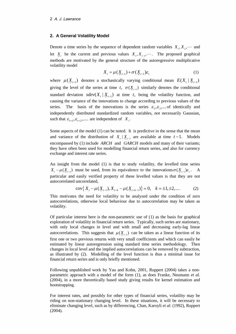
A plot of the FTSE100 index series , 1, 2,...,1542t
I t is given by the upper trace in
Figure 1, and the lower trace is the corresponding return series1 1
( ) .t t t
I I I
This is
Volatility Graphics 5
01/01/201101/01/201001/01/200901/01/200801/01/200701/01/200601/01/2005
8000
7000
6000
5000
4000
10%
5%
0%
-5%
-10%
Daily Date
Retu
rns
FT
SE
Valu
es
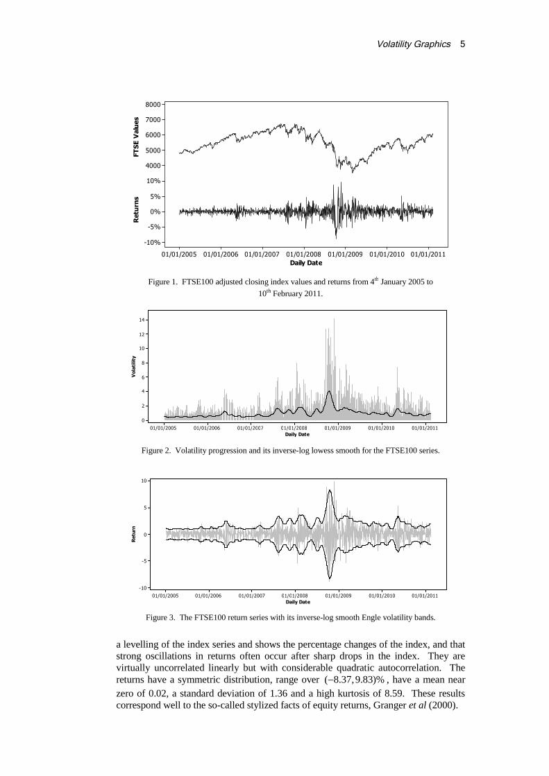
Figure 1. FTSE100 adjusted closing index values and returns from 4th January 2005 to
10th February 2011.
01/01/201101/01/201001/01/200901/01/200801/01/200701/01/200601/01/2005
14
12
10
8
6
4
2
0
Daily Date
Vola
tility
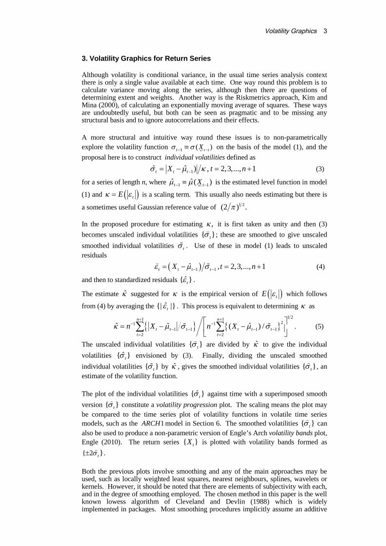
Figure 2. Volatility progression and its inverse-log lowess smooth for the FTSE100 series.
01/01/201101/01/201001/01/200901/01/200801/01/200701/01/200601/01/2005
10
5
0
-5
-10
Daily Date
Retu
rn
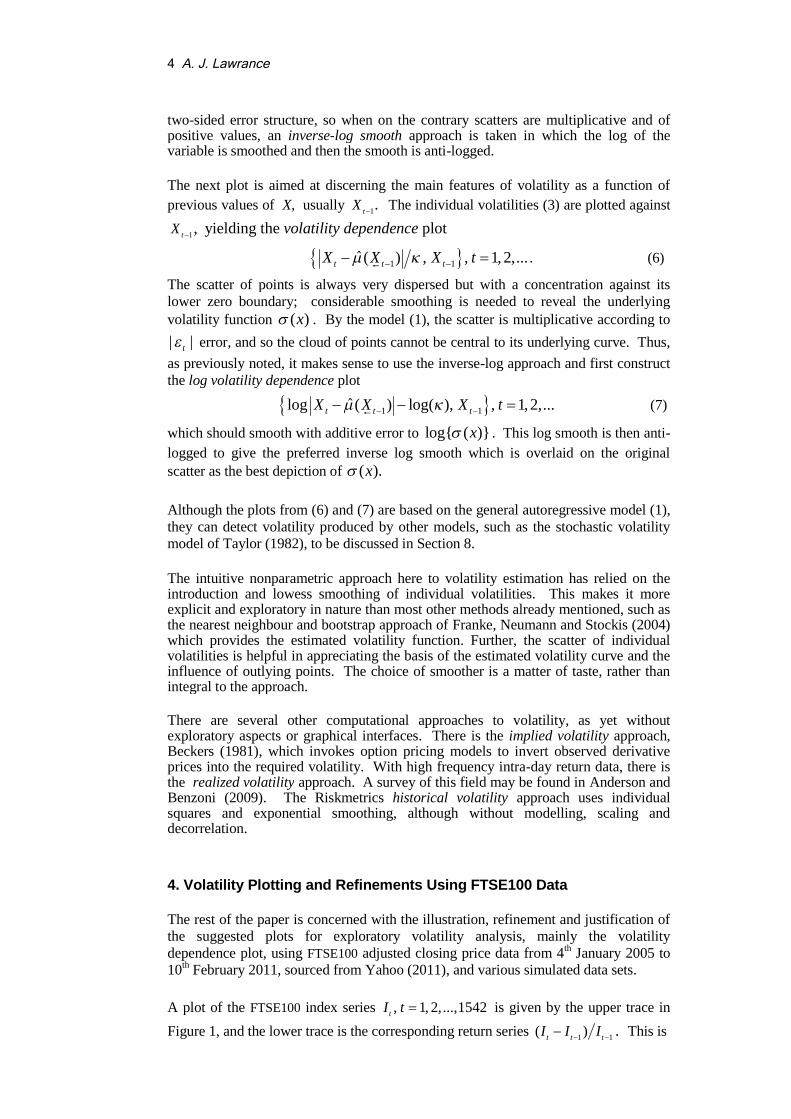
Figure 3. The FTSE100 return series with its inverse-log smooth Engle volatility bands.
a levelling of the index series and shows the percentage changes of the index, and thatstrong oscillations in returns often occur after sharp drops in the index. They arevirtually uncorrelated linearly but with considerable quadratic autocorrelation. Thereturns have a symmetric distribution, range over ( 8.37,9.83)% , have a mean near
zero of 0.02, a standard deviation of 1.36 and a high kurtosis of 8.59. These resultscorrespond well to the so-called stylized facts of equity returns, Granger et al (2000).
6 A. J. Lawrance
6420-2-4-6
10
8
6
4
2
1
0
Previous Return
Vola
tility
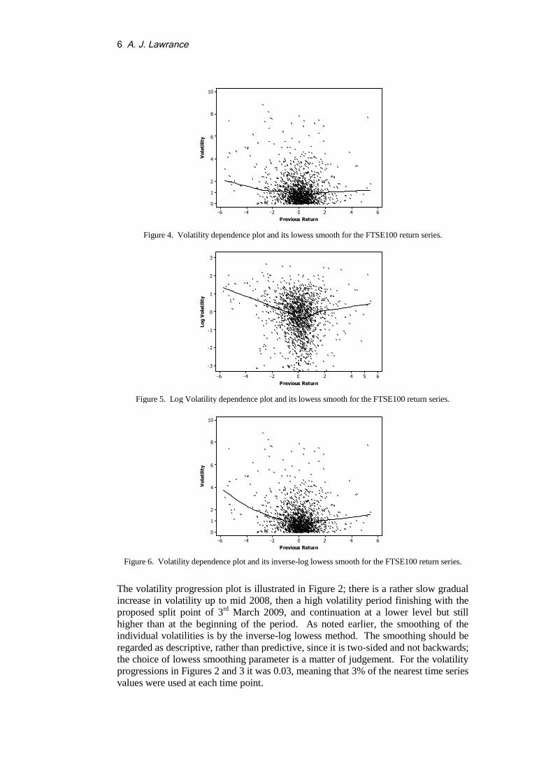
Figure 4. Volatility dependence plot and its lowess smooth for the FTSE100 return series.
65420-2-4-6
3
2
1
0
-1
-2
-3
Previous Return
Log
Vola
tility
Figure 5. Log Volatility dependence plot and its lowess smooth for the FTSE100 return series.
Figure 6. Volatility dependence plot and its inverse-log lowess smooth for the FTSE100 return series.
The volatility progression plot is illustrated in Figure 2; there is a rather slow gradualincrease in volatility up to mid 2008, then a high volatility period finishing with theproposed split point of 3rd March 2009, and continuation at a lower level but stillhigher than at the beginning of the period. As noted earlier, the smoothing of theindividual volatilities is by the inverse-log lowess method. The smoothing should beregarded as descriptive, rather than predictive, since it is two-sided and not backwards;the choice of lowess smoothing parameter is a matter of judgement. For the volatilityprogressions in Figures 2 and 3 it was 0.03, meaning that 3% of the nearest time seriesvalues were used at each time point.
6420-2-4-6
10
8
6
4
2
1
0
Previous Return
Vola
tility
Volatility Graphics 7
6420-2-4-6
12
10
8
6
4
2
1
0
Previous Model-Residual
Vola
tility
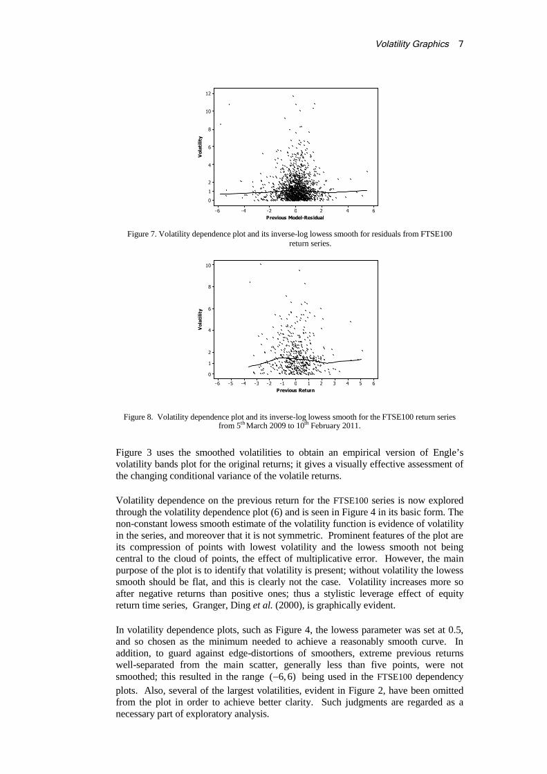
Figure 7. Volatility dependence plot and its inverse-log lowess smooth for residuals from FTSE100return series.
6543210-1-2-3-4-5-6
10
8
6
4
2
1
0
Previous Return
Vola
tility
Figure 8. Volatility dependence plot and its inverse-log lowess smooth for the FTSE100 return seriesfrom 5th March 2009 to 10th February 2011.
Figure 3 uses the smoothed volatilities to obtain an empirical version of Engle’svolatility bands plot for the original returns; it gives a visually effective assessment ofthe changing conditional variance of the volatile returns.
Volatility dependence on the previous return for the FTSE100 series is now exploredthrough the volatility dependence plot (6) and is seen in Figure 4 in its basic form. Thenon-constant lowess smooth estimate of the volatility function is evidence of volatilityin the series, and moreover that it is not symmetric. Prominent features of the plot areits compression of points with lowest volatility and the lowess smooth not beingcentral to the cloud of points, the effect of multiplicative error. However, the mainpurpose of the plot is to identify that volatility is present; without volatility the lowesssmooth should be flat, and this is clearly not the case. Volatility increases more soafter negative returns than positive ones; thus a stylistic leverage effect of equityreturn time series, Granger, Ding et al. (2000), is graphically evident.
In volatility dependence plots, such as Figure 4, the lowess parameter was set at 0.5,and so chosen as the minimum needed to achieve a reasonably smooth curve. Inaddition, to guard against edge-distortions of smoothers, extreme previous returnswell-separated from the main scatter, generally less than five points, were notsmoothed; this resulted in the range ( 6, 6) being used in the FTSE100 dependency
plots. Also, several of the largest volatilities, evident in Figure 2, have been omittedfrom the plot in order to achieve better clarity. Such judgments are regarded as anecessary part of exploratory analysis.
8 A. J. Lawrance
Figure 5 repeats the plot in Figure 4 using volatility on the log scale and avoidscompression of the scatter, as previously asserted.
The inverse of the log lowess smooth from Figure 5 is now used to replace the lowesssmooth in Figure 4. This results in Figure 6, the preferred version of the volatilitydependence plot.
The practical message from Figure 6 is a refinement of that from Figure 3, namely thatthere is evidence for asymmetric volatility of the FTSE100 returns, with a tendency ofhigh volatility to follow low return when considered over the over the period 4th
January 2005 to 10th February 2011. Although this plot is fairly convincing, it isnatural to take the residuals from the model (1), as defined at (4), and examine themfor remaining volatility. In the case of the FTSE100 series, Figure 7 indicates clearlythat this is not the case.
Further similar analysis to that given by Figures 4-7 was under taken for prior- andpost- 4th March 2009, a proxy for the supposed end of recession. Essentially the sameresults were obtained for the data up to the 4th March. From the 5th March onwardsvery different results were obtained, as shown in the volatility dependence plot inFigure 8; first, the range of returns is much smaller, within 5% and secondly, thereis now hardly any evidence of volatility, a previously very unusual situation in aperiod of 488 trading days. This did, however, accord with current market perceptionsat the time.
5. Bootstrap Validation of Volatility Dependence Plots
There could be concern for the validity of volatility dependence plots in respect ofunderlying statistical variation associated with them. Thus, there is a further need foran uncertainty assessment of the lowess smoothed volatility function. While thiswould be a complicated or intractable task to achieve formally, an exploratorynonparametric bootstrap approach is a practical response. In this approach, the
FTSE100 smoothed volatilities { }t
were used as the estimated volatility function in
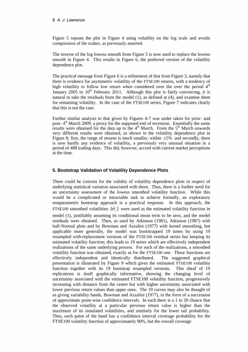
model (1), justifiably assuming its conditional mean term to be zero, and the modelresiduals were obtained. Then, as used by Atkinson (1981), Atkinson (1987) withhalf-Normal plots and by Bowman and Azzalini (1977) with kernel smoothing, butapplicable more generally, the model was bootstrapped 19 times by using 19resampled with-replacement versions of the FTSE100 residual series but keeping itsestimated volatility function; this leads to 19 series which are effectively independentrealizations of the same underlying process. For each of the realizations, a smoothedvolatility function was obtained, exactly as for the FTSE100 one. These functions areeffectively independent and identically distributed. The suggested graphicalpresentation is illustrated by Figure 9 which gives the estimated FTSE100 volatilityfunction together with its 19 bootstrap resampled versions. This sheaf of 19replications is itself graphically informative, showing the changing level ofuncertainty associated with the estimated FTSE100 volatility function, progressivelyincreasing with distance from the centre but with higher uncertainty associated withlower previous return values than upper ones. The 19 curves may also be thought ofas giving variability bands, Bowman and Azzalini (1977), in the form of a successionof approximate point-wise confidence intervals. In each there is a 1 in 20 chance thatthe observed volatility at a particular previous return value is higher than themaximum of its simulated volatilities, and similarly for the lower tail probability.Thus, each point of the band has a confidence interval coverage probability for theFTSE100 volatility function of approximately 90%, but the overall coverage

Volatility Graphics 9
6420-2-4-6
10
8
6
4
2
1
0
Previous Return
Vola
tility
Figure 9. Volatility dependence plot and its inverse-log lowess smooth (dark line) for the FTSE100return series and 19 bootstrap versions.
6420-2-4-6
10
8
6
4
2
1
0
Previous Return
Vola
tility
Figure 10. Volatility dependence plot and its inverse-log lowess smooth (dark line) for the FTSE100return series and a sheaf of 19 volatility curves of the resampled model residuals.
probability is not easy to assess in a simple way. However, the main importance ofthe graphics is to provide guidance as to what are extreme fluctuations.
Although the previous volatility curve estimate and its bootstrap uncertainty analysisgive quite compelling evidence that the FTSE100 series exhibits asymmetricvolatility, the same resampling approach can also be used to provide a graphically-based informal test of the hypothesis that there is no volatility. Instead of creating 19bootstrap resamplings using the estimated FTSE100 volatility function, a constantvolatility function is used, corresponding to the null hypothesis of no volatility,together, with 19 resampled sets of FTSE100 residuals. A sheaf of 19 resampledvolatility functions is thus obtained, exactly as before. Figure 10 shows these togetherwith the originally estimated FTSE100 volatility function. It is quite clear that the nullhypothesis is untenable and additionally that the evidence comes mainly from the lowreturns. The informal significance level of the point-wise tests follows as 10%according to the previous arguments. Once again, graphical evidence from the sheafof 19 resamplings provides a good indication as to what can be considered extreme.
10 A. J. Lawrance
6420-2-4-6
12
10
8
6
4
2
1
0
Previous Value
Vola
tility
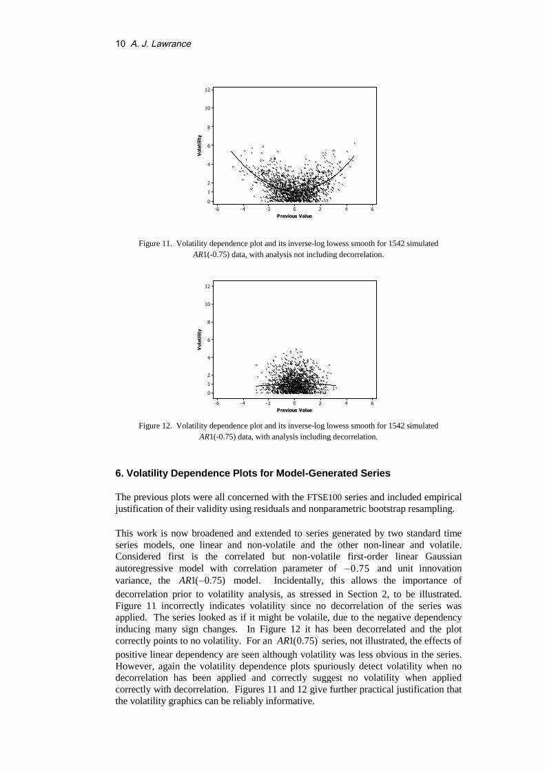
Figure 11. Volatility dependence plot and its inverse-log lowess smooth for 1542 simulated
AR1(-0.75) data, with analysis not including decorrelation.
6420-2-4-6
12
10
8
6
4
2
1
0
Previous Value
Vola
tility
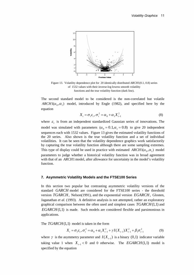
Figure 12. Volatility dependence plot and its inverse-log lowess smooth for 1542 simulated
AR1(-0.75) data, with analysis including decorrelation.
6. Volatility Dependence Plots for Model-Generated Series
The previous plots were all concerned with the FTSE100 series and included empiricaljustification of their validity using residuals and nonparametric bootstrap resampling.
This work is now broadened and extended to series generated by two standard timeseries models, one linear and non-volatile and the other non-linear and volatile.Considered first is the correlated but non-volatile first-order linear Gaussianautoregressive model with correlation parameter of 0.75 and unit innovationvariance, the 1( 0.75)AR model. Incidentally, this allows the importance of
decorrelation prior to volatility analysis, as stressed in Section 2, to be illustrated.Figure 11 incorrectly indicates volatility since no decorrelation of the series wasapplied. The series looked as if it might be volatile, due to the negative dependencyinducing many sign changes. In Figure 12 it has been decorrelated and the plotcorrectly points to no volatility. For an 1(0.75)AR series, not illustrated, the effects of
positive linear dependency are seen although volatility was less obvious in the series.However, again the volatility dependence plots spuriously detect volatility when nodecorrelation has been applied and correctly suggest no volatility when appliedcorrectly with decorrelation. Figures 11 and 12 give further practical justification thatthe volatility graphics can be reliably informative.
Volatility Graphics 11
6420-2-4-6
12
10
8
6
4
2
1
0
Previous Value
Vola
tility
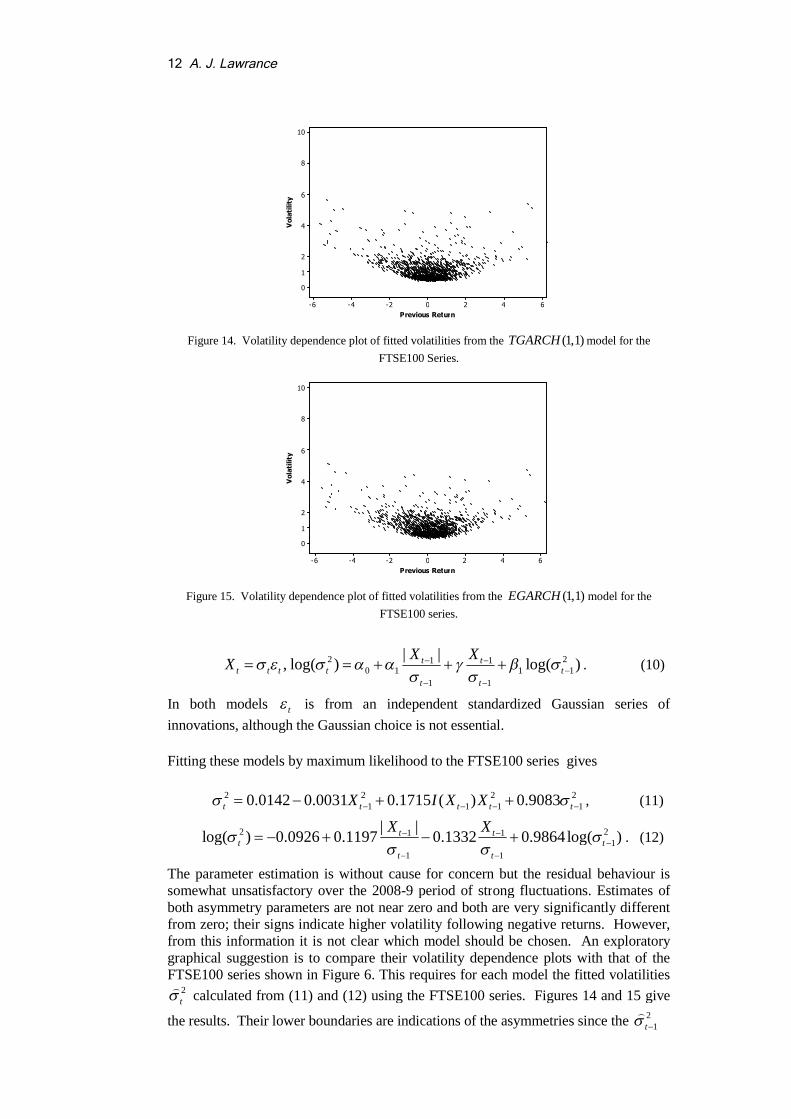
Figure 13. Volatility dependence plot for 20 identically distributed ARCH1(0.1, 0.8) series
of 1532 values with their inverse-log lowess smooth volatility
functions and the true volatility function (dark line).
The second standard model to be considered is the non-correlated but volatile
0 11( ),ARCH model, introduced by Engle (1982), and specified here by the
equation2 2
0 1 1,t t t t tX X (8)
where t is from an independent standardized Gaussian series of innovations. The
model was simulated with parameters 0 1( )0.1, 0.8 to give 20 independent
sequences each with 1532 values. Figure 13 gives the estimated volatility functions ofthe 20 series. Also shown is the true volatility function and a set of individualvolatilities. It can be seen that the volatility dependence graphics work satisfactorilyby capturing the true volatility function although there are some sampling extremes.
This type of display could be used in practice with estimated 0 11( ),ARCH model
parameters to judge whether a historical volatility function was in broad agreementwith that of an 1ARCH model, after allowance for uncertainty in the model’s volatilityfunction.
7. Asymmetric Volatility Models and the FTSE100 Series
In this section two popular but contrasting asymmetric volatility versions of thestandard GARCH model are considered for the FTSE100 series - the threshold
version ,TGARCH Nelson(1991), and the exponential version ,EGARCH Glosten,
Jaganathan et al. (1993). A definitive analysis is not attempted, rather an exploratorygraphical comparison between the often used and simplest cases (1,1)TGARCH and
(1,1)EGARCH is made. Such models are considered flexible and parsimonious in
applications.
The (1,1)TGARCH model is taken in the form
2 2 2 20 1 1 1 1 1 1, ( )t t t t t t t tX X I X X (9)
where is the asymmetry parameter and 1( )tI X is a binary (0,1) indicator variable
taking value 1 when 1 0tX and 0 otherwise. The (1,1)EGARCH model is
specified by the equation
12 A. J. Lawrance
6420-2-4-6
10
8
6
4
2
1
0
Previous Return
Vola
tility
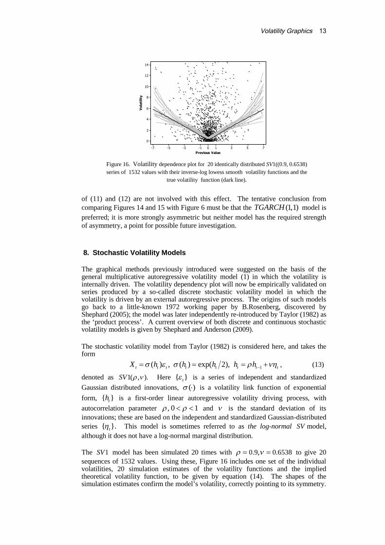
Figure 14. Volatility dependence plot of fitted volatilities from the (1,1)TGARCH model for the
FTSE100 Series.
6420-2-4-6
10
8
6
4
2
1
0
Previous Return
Vola
tility
Figure 15. Volatility dependence plot of fitted volatilities from the (1,1)EGARCH model for the
FTSE100 series.
2 21 10 1 1 1
1 1
| |, log( ) log( )t t
t t t t t
t t
X XX
. (10)
In both models t is from an independent standardized Gaussian series of
innovations, although the Gaussian choice is not essential.
Fitting these models by maximum likelihood to the FTSE100 series gives
2 2 2 21 1 1 10.0142 0.0031 0.1715 ( ) 0.9083t t t t tX I X X , (11)
2 21 11
1 1
| |log( ) 0.0926 0.1197 0.1332 0.9864log( )t t
t t
t t
X X
. (12)
The parameter estimation is without cause for concern but the residual behaviour issomewhat unsatisfactory over the 2008-9 period of strong fluctuations. Estimates ofboth asymmetry parameters are not near zero and both are very significantly differentfrom zero; their signs indicate higher volatility following negative returns. However,from this information it is not clear which model should be chosen. An exploratorygraphical suggestion is to compare their volatility dependence plots with that of theFTSE100 series shown in Figure 6. This requires for each model the fitted volatilities
2t
calculated from (11) and (12) using the FTSE100 series. Figures 14 and 15 give
the results. Their lower boundaries are indications of the asymmetries since the 21t
Volatility Graphics 13
75310-1-3-5-7
14
12
10
8
6
4
2
0
Previous Value
Vola
tility
Figure 16. Volatility dependence plot for 20 identically distributed SV1((0.9, 0.6538)
series of 1532 values with their inverse-log lowess smooth volatility functions and the
true volatility function (dark line).
of (11) and (12) are not involved with this effect. The tentative conclusion fromcomparing Figures 14 and 15 with Figure 6 must be that the (1,1)TGARCH model is
preferred; it is more strongly asymmetric but neither model has the required strengthof asymmetry, a point for possible future investigation.
8. Stochastic Volatility Models
The graphical methods previously introduced were suggested on the basis of thegeneral multiplicative autoregressive volatility model (1) in which the volatility isinternally driven. The volatility dependency plot will now be empirically validated onseries produced by a so-called discrete stochastic volatility model in which thevolatility is driven by an external autoregressive process. The origins of such modelsgo back to a little-known 1972 working paper by B.Rosenberg, discovered byShephard (2005); the model was later independently re-introduced by Taylor (1982) asthe ‘product process’. A current overview of both discrete and continuous stochasticvolatility models is given by Shephard and Anderson (2009).
The stochastic volatility model from Taylor (1982) is considered here, and takes theform
1( ) , ( ) exp( 2),t t t t t t t tX h h h h h , (13)
denoted as 1( , ).SV Here { }t is a series of independent and standardized
Gaussian distributed innovations, ( ) is a volatility link function of exponential
form, { }th is a first-order linear autoregressive volatility driving process, with
autocorrelation parameter , 0 1 and is the standard deviation of its
innovations; these are based on the independent and standardized Gaussian-distributed
series { }.t This model is sometimes referred to as the log-normal SV model,
although it does not have a log-normal marginal distribution.
The 1SV model has been simulated 20 times with 0.9 0.6538, to give 20
sequences of 1532 values. Using these, Figure 16 includes one set of the individualvolatilities, 20 simulation estimates of the volatility functions and the impliedtheoretical volatility function, to be given by equation (14). The shapes of thesimulation estimates confirm the model’s volatility, correctly pointing to its symmetry.
14 A. J. Lawrance
The 1SV model is a two-equation time series model with two innovation variables t
and t , and does not explicitly relate current value to past values as with single-
equation models; therefore it can not be directly compared to models in the
autoregressive volatility family (1). It is instructive therefore to use (13) to relate tX
and 1tX by eliminating th and 1th between their two equations; then there is the
alternative representation
1 1| | exp( 2) .t t t t tX X (14)
This demonstrates that the 1SV model has first-order autoregressive volatility
function 1| |tX but that the innovations 1exp( 2)t t t
are formed from the
two IID series of innovations and are dependent. Due to this structure it is not amember of the autoregressive volatility family (1). Further, its volatility function is
not continuous at 1 0tX , although a smooth approximation has been given by
lowess smoothing in Figure 16.
A useful feature of the representation (14) is afforded by its logarithmic-absolute valuetransformation which brings it to be the linear model
11 12log | | log | | log | | log | |,t t t t tX X (15)
but with two innovation variables. Thus, the logarithmic-absolute valuetransformation eliminates volatility from the 1SV model. This is a helpful feature indata analysis since using the volatility dependence plot on both the untransformed andtransformed data could give evidence for the suitability or not of an 1SV model.
9. A Theoretical Illustration of Volatility Decorrelation
As just seen in Section 8, in a multiple-equation time series model, the volatilityfunction may be implicit rather than explicit. Another such case is the first-orderautoregressive (1)AR model with (1)ARCH innovations. This is an autocorrelated
volatility model. Thus, suppose
1t t tX X e (16)
where the innovations { }te are generated by the (1)ARCH model
20 1 1t t te e . (17)
The { }t are independent and identically distributed. A single-equation form of this
model is obtained by setting 1t t te X X in (17) and becomes
21 0 1 1 2( )t t t t tX X X X . (18)
This is in the class of models (1) where there is a level term and the volatility is now afunction of the two immediately past values; hence the volatility dependence scatterwould be in three dimensions and need a smoothing surface. However, it is pertinent
to note that the volatility function of (18) involves the decorrelated1t
X
values, so
alternatively, the series could be decorrelated initially, and the decorrelated valuesused as ARCH1 values in the volatility dependence plots (6) and (7). In effect, this is aparametric version of the non-parametric decorrelation strategy.
Volatility Graphics 15
10. Discussion
The proposed graphics can be applied to many types of financial time series as well asindex returns, such as individual equity returns, portfolio returns, exchange rates andinterest rates, and to other time series areas requiring volatility analysis. The behaviourof volatility dependence has been found to vary with the area of application. Inregard to interest rates, there is some evidence that differenced series point toincreased volatility after substantially increased rates.
There are a number of possible extensions to the proposed methods. Empiricalexperience suggests that volatility dependence plots can also be univariately effectivewith the previous two or three values. They could also be extended to jointly explorea volatility surface in terms of the previous two values. The extent of practical gainfrom more sophisticated non-parametric methods of volatility estimation could beinvestigated. Higher order multiplicative autoregressive representations of stochasticvolatility models offer further model-checking developments. Other extensions, suchas generalizations to vector time series, should also be possible.
References
Anderson, T.G. and Benzoni, K. (2009) Realized volatility, in Handbook of Financial TimeSeries, Ed. T.G. Anderson , R.A. Davis , J.-P. Kreiss and T. Mikosch, Heidelberg: Springer-Verlag.
Anderson, T.G., Davies, R.A., Kreiss, J.P. and Mikosch, T. (2009) Handbook of FinancialTime Series: Springer-Verlag.
Atkinson, A.C. (1981) Two graphical displays for outlying and influential observations inregression, Biometrika, 68, 13-20.
Atkinson, A.C. (1987) Plots, Transformations and Regression, Oxford: Clarendon Press.
Beckers, S. (1981) Standard deviations implied in option prices as predictors of future stockprice variability, Journal of Banking and Finance, 5, 363-381.
Bowman, A.W. and Azzalini, A. (1977) Applied Smoothing Techniques for Data Analysis,Oxford: Clarendon Press.
Chan, C., Karoyli, G.A., Longstaff, F.A. and Sanders, A.B. (1992) An empirical comparisonof alternative models for short term interest rates, Journal of Finance, XLVII, 1209-1277.
Cleveland, W.S. and Devlin, S.J. (1988) Locally-weighted regression: An approach toregression analysis by local fitting, Journal of the American Statistical Association, 83, 596-610.
Engle, R.F. (1982) Autoregressive conditional heteroscedasticity with estimates of thevariance of United Kingdom inflation, Econometrica, 50, 987-1008.
Engle, R.F. (2010) Robert Engle's FT Lectures on Volatility, parts 1-5:http://readingthemarkets.blogspots.com/2010/09/robert-engles-ft-lectures.
Fan, J. and Yao, Q. (2003) Nonlinear Time Series, New York: Springer.
Franke, J., Neumann, M.H. and Stockis, J.-P. (2004) Bootstrapping nonparametric estimatorsof the volatility function, Journal of Econometrics, 118, 189-218.
Glosten, L.R., Jaganathan, R. and Runkle, D. (1993) On the relation between expected valueand volatility of the normal excess return on stocks, Journal of Finance, 48, 1779-1801.

16 A. J. Lawrance
Granger, C.W., Ding, Z. and Spear, S. "Stylized facts on the temporal and distributionalproperties of absolute returns: an update," Presented at Hong Kong International Workshopon Statistics and Finance: An Interface, 2000, Eds., London: Imperial College Press.
Kim, J. and Mina, J. (2000) Riskgrades Technical Document, New York: Riskmetrics.
Ruppert, D. (2004) Statistics and Finance: An Introduction, New York: Springer.
Shephard, N. (2005) Stochastic Volatility: Selected Readings: Oxford University Press.
Shephard, N. and Anderson, T.G. (2009) Stochastic volatility: origins and overview, inHandbook of Financial Time Series, Ed. T.G. Anderson , R.A. Davis , J.-P. Kreiss and T.Mikosch, Heidelberg: Springer-Verlag, 233-254.
Taylor, S.J. (1982) Financial returns modelled by the product of two stochastic processes - astudy of daily sugar prices 1961-79, in Time Series Analysis: Theory and Practice, Ed. O.D.Anderson, Amsterdam: North-Holland, 203-226.
Yahoo (2011) FTSE100 historical prices:http://finance.yahoo.com/q/hp?s=%5EFTSE+Historical+Prices.