Embed Size (px)
Citation preview

HAL Id: hal-01527222https://hal.archives-ouvertes.fr/hal-01527222
Submitted on 24 May 2017
HAL is a multi-disciplinary open accessarchive for the deposit and dissemination of sci-entific research documents, whether they are pub-lished or not. The documents may come fromteaching and research institutions in France orabroad, or from public or private research centers.
L’archive ouverte pluridisciplinaire HAL, estdestinée au dépôt et à la diffusion de documentsscientifiques de niveau recherche, publiés ou non,émanant des établissements d’enseignement et derecherche français ou étrangers, des laboratoirespublics ou privés.
Exploratory spatial data analysis of the distribution ofregional per capita GDP in Europe, 1980-1995
Julie Le Gallo, Cem Ertur
To cite this version:Julie Le Gallo, Cem Ertur. Exploratory spatial data analysis of the distribution of regional percapita GDP in Europe, 1980-1995. [Research Report] Laboratoire d’analyse et de techniqueséconomiques(LATEC). 2000, 25 p., Graph, ref. bib. : 29 ref. �hal-01527222�

LABORATOIRE D'ANALYSE ET DE TECHNIQUES ÉCONOMIQUES
UMR5118 CNRS
DOCUMENT DE TRAVAIL
CENTRE NATIONAL DE LA RECHERCHE SCIENTIFIQUE
Pôle d'Économie et de Gestion
UNIVERSITE DE BOURGOGNE
2, bd Gabriel- BP 26611 - F -21066 Dijon cedex - Tél. 03 80 39 54 30 - Fax 03 80 39 5443
Courrier électronique: [email protected]
ISSN : 1260-8556

n° 2000-09
Exploratory spatial data analysis of the distribution of regional per capita GDP in Europe, 1980-1995
Julie LE GALLO, Cem ERTUR
August 2000
e-mail : JleGallo(cb,aol. com
Cem. ErturdcÒM-bourzozne. fr
Website :http://www.u-bourgogne.fr/LATEC
Previous versions of this paper were presented at the 6*h RSAI World Congress 2000 “Regional Science in a Small World”, Lugano, Switzerland, May 16-20, 2000 and 40*ERSA Congress “European Monetary Union and Regional Policy”, Barcelona, Spain, 29 August - 1 September, 2000. We would like to thank R. Florax and C. Baumont for their helpful comments. Any errors or omissions remain our responsibility.
Exploratory Spatial Data Analysis of the distribution ofregional per capita GDP in Europe, 1980-1995
Abstract. The aim of this paper is to study the dynamics of European regional per capita product over time and space. This purpose is achieved by using the recently developed methods of Exploratory Spatial Data Analysis. Using a sample of European regions over the 1980-1995 period, we find strong evidence of global and local spatial autocorrelation in per capita GDP throughout the period. The detection of clusters of high and low per capita products during the period is an indication of the persistence of spatial disparities between European regions. This analysis is finally refined by the investigation of the spatial pattern of regional growth.
JEL classification: C21,018, 052, RII, R12
Key words: exploratory spatial data analysis, distribution of regional per capita GDP, European Union, spatial autocorrelation, regional inequalities
1 Introduction
The integration of the European market has stimulated the analysis of regional economic
convergence within the European Union in the recent macroeconomic literature (Neven and
Gouyette 1995; Abraham and Von Rompuy 1995; Armstrong 1995; Molle and Broeckhout
1995). Most of the time, the empirical methods that have been used are identical to the
methods used in international studies. However, at the regional scale, spatial effects and
particularly spatial autocorrelation are determining for the analysis of convergence processes.
Several factors, like trade between regions, technology and knowledge diffusion and more
generally regional externalities and spillovers, lead to geographically dependent regions: there
are spatial interactions between regions and the geographical location plays an important role.
Despite their importance, the role of spatial effects in convergence processes has been only
2

recently examined using spatial statistics and spatial econometric methods (Lopez-Bazo et al.
1999; Fingleton 1999; Rey and Montouri 1999).
Therefore, this paper aims at studying the dynamics of European regional per capita
product over time and space. In this purpose, we use the recently developed methods of
Exploratory Spatial Data Analysis to examine the spatial distribution of regional per capita
products. The detection of global and local spatial autocorrelation enables to characterize the
way the economic activities are located in the European Union and the way this pattern of
location has changed over the period.
In the second section, we briefly present the principles and methods of Exploratory
Spatial Data Analysis (ESDA). Using a sample of European regions over the 1980-1995
period, we compute in the third section a global spatial autocorrelation statistic, as well as
local Moran autocorrelation statistics (Moran scatterplot and LISA; Anselin 1995, 1996) in
order to detect clusters of high and low per capita products. Indeed, the existence of those
clusters during the period would be an indication of the persistence of spatial disparities
between European regions. The spatial pattern of regional growth is finally investigated.
2 Exploratory Spatial Data Analysis
Exploratory Spatial Data Analysis (ESDA) is a set of techniques aimed at describing
and visualizing spatial distributions, at identifying atypical localizations or spatial outliers, at
detecting patterns of spatial association, clusters or hot spots, and at suggesting spatial
regimes or other forms of spatial heterogeneity (Haining 1990; Bailey and Gatrell 1995;
Anselin 1998a, 1998b). These methods provide measures of global and local spatial
autocorrelation.
2. 1 Global spatial autocorrelation
Spatial autocorrelation can be defined as the coincidence of value similarity with
locational similarity (Anselin 2000). Therefore there is positive spatial autocorrelation when
high or low values of a random variable tend to cluster in space and there is negative spatial

autocorrelation when geographical areas tend to be surrounded by neighbors with very
dissimilar values.
The measurement of global spatial autocorrelation is based on the Moran’s I statistic,
which is the most widely known measure of spatial clustering (Cliff and Ord 1973, 1981;
Upton and Fingleton 1985; Haining 1990). For each year of the period 1980-1995, this
statistic is written in the following way:
where xit is the observation in region i and year t , fut is the mean of the observations across
regions in year t . n is the number of regions. Wy is the element of the spatial weight matrix
W . This matrix contains the information about the relative spatial dependence between the n
regions i . The elements wu on the diagonal are set to zero whereas the elements indicate
the way region i is spatially connected to the region j . Finally, S0 is a scaling factor equal to
the sum of all the elements of W .
The spatial weight matrix we use in this study is based on the 10 nearest neighbors
calculated from the great circle distance between region centroids. In Europe, regions have on
average 5 to 6 contiguous neighbors, our choice of 10 yields a ring around each region of
approximately the first and second order contiguous regions and moreover connects United-
Kingdom as well as some islands such as Sicilia, Sardegna, and Baleares to continental
Europe. Furthermore, it also connects Greece to Italy, so that the block-diagonal structure of
the simple contiguity matrix is avoided. This feature is of particular interest when working on
a sample of European regions, which are less compact than US states.
Noting z, the vector of the n observations for year t in deviation from the mean /ut ,
(1) can be written in the following matrix form:
(1)
4

In order to normalize the outside influence upon each region, the spatial weight matrix
is row-standardized such that the elements in each row sum to 1. In this case, the expression
(2) simplifies since for row-standardized weights S0=n.
Moran’s I statistic gives a formal indication on the degree of linear association between
the vector z, of observed values and the vector Wz, of spatially weighted averages of
neighboring values, called the spatially lagged vector. Values of I larger than the expected
value E( l ) = - l /(n - l ) indicate positive spatial autocorrelation, while values smaller than the
expected indicate negative spatial autocorrelation. Inference is based on the permutation
approach with 10000 permutations. In this approach, it is assumed that, under the null
hypothesis, each observed value could have occurred at all locations with equal likelihood.
But instead of using the theoretical mean and standard deviation (given by Cliff and Ord
1981), a reference distribution is empirically generated for I, from which the mean and
standard deviation are computed. In practice this is carried out by permuting the observed
values over all locations and by re-computing I for each new sample. The mean and standard
deviation for I are then the computed moments for the reference distribution for all
permutations (Anselin 1995).
2.2 Local spatial autocorrelation
Moran’s I statistic is a global statistic: it does not enable us to appreciate the regional
structure of spatial autocorrelation. However, one can wonder which regions contribute more
to the global spatial autocorrelation, if there are local spatial clusters of high or low values,
and finally to what point the global evaluation of spatial autocorrelation masks atypical
localizations or “pockets of local nonstationarity”, i.e. respectively regions or groups of
contiguous regions, which deviate from the global pattern of positive spatial autocorrelation.

The analysis of local spatial autocorrelation is carried out with two tools: first, the
Moran scatterplot (Anselin 1996), which is used to visualize local spatial instability, and
second, local indicators of spatial association “LISA” (Anselin 1995), which are used to test
the hypothesis of random distribution by comparing the values of each specific localization
with the values in the neighboring localizations.
Moran Scatterplot
Inspection of local spatial instability is carried out by the means of the Moran scatterplot
(Anselm 1996), which plots the spatial lag Wz, against the original values z , . The four
different quadrants of the scatterplot correspond to the four types of local spatial association
between a region and its neighbors: (HH) a region with a high1 value surrounded by regions
with high values (Quadrant I in top on the right), (LH) a region a with low value surrounded
by regions with high values (Quadrant II in top on the left), (LL) a region with a low value
surrounded by regions with low values (Quadrant III in bottom on the left), (HL) a region with
a high value surrounded by /regions with low values (Quadrant IV in bottom on the right).
Quadrants I and IE refer to positive spatial autocorrelation indicating spatial clustering of
similar values whereas quadrants II and IV represent negative spatial autocorrelation
indicating spatial clustering of dissimilar values. The Moran scatterplot may thus be used to
visualize atypical localizations, i.e. regions in quadrant II or in the quadrant IV. Moreover, the
use of standardized variables allows the Moran scatterplots to be comparable across time.
The global spatial autocorrelation may also be visualized in this graph since, from (2)
Moran’s I is formally equivalent to the slope coefficient of the linear regression of Wz, on
z, using a row-standardized weight matrix. Therefore, this regression can be assessed with
diagnostics for model fit. The detection of outliers and sites, which exert strong influence on
Moran’s I, is based on standard regression diagnostics: studentized residuals and leverage
measures are used to detect outliers, and Cook’s distance is an influence measure (Belsley et
al. 1980; Haining 1994,1995). The studentized residual is a measure of the extreme character
6

of an observation along the dependent variable domain and is calculated as the studentized
difference between the actual value and the predicted value. The leverage quantifies the
extreme nature of an observation in the range of the independent variable and is assessed
using the diagonal elements of the hat matrix2 (Haoglin and Welsch 1978). Finally, the
Cook’s distance combines the two previous diagnostics and measures the extent to which
regression coefficients are changed by the deletion of a particular observation (Cook 1977;
Weisberg 1985).
Let us note however that the Moran scatterplot does not give any indications of
significant spatial clustering and therefore, it cannot be considered as a Local Indicator of
Spatial Association in the sense defined by Anselin (1995).
Local indicators of spatial association (LISA)
Anselin (1995) defines a local indicator of spatial association as any statistics satisfying
two criteria3. First, the LISA for each observation gives an indication of significant spatial
clustering of similar values around that observation; second, the sum of the LISA for all
observations is proportional to a global indicator of spatial association.
The local version of the Moran’s I statistic for each region i and year t can then be
written as following:
where the summation over j is such that only neighboring values of j are included. It is
straightforward to see that the sum of local Moran’s statistics can be written:
1 High (respectively low) means above (respectively below) the mean.2 The hat matrix is defined as H = X(X'X)~' X' where X is the matrix of observations on the explanatory variables in a regression.3 Note that the Getis and Ord (1992) local statistics G,(d) and G' (if) are not LISAs in the sense defined byAnselin (1995) since they are not related to a global statistic of spatial association and will not be used in this study.
(3)

From (1), it follows that the global Moran’s / statistic is proportional to the sum of local
Moran’s statistics:
',=2X./S° <5)
For a row-standardized weight matrix, S0=n so that /, = —V : the global Moran’s /n i '
equals the mean of the local Moran’s statistics. A positive value for , indicates clustering of
similar values (high or low) whereas a negative value indicates clustering of dissimilar values.
Due to the presence of global spatial autocorrelation, inference must be based on the
conditional permutation approach: the value xi at site i is held fixed, while the remaining
values are randomly permuted over all locations (note that only the quantity (x,, ~M<)
needs to be computed for each permutation since the term (jc( , ~M,)/mo remains constant for
a given region i ). It should be stressed that p -values obtained for the local Moran’s statistics
are actually pseudo-significance levels. Inference is further complicated by the fact that local
Moran’s statistics will be correlated when the neighborhood sets of two regions contain
common elements (Ord and Getis 1995; Anselin 1995). This is actually a problem of multiple
statistical comparison and the significance levels must be approximated by the Bonferroni
inequality or by the procedure elaborated by Sidak (1967)4. As noted by Anselin (1995, p.96):
“This means that when the overall significance associated with the multiple comparisons
(correlated tests) is set to a , and there are m comparisons, then the individual significance a,
should be set to a/m (Bonferroni) or l - ( l - a ) 1/m (Sidak)”. With m = n, the number of
regions of the sample, these procedures can be overly conservative to assess the significance
of local Moran’s statistics. The second procedure requires that the variables are multivariate
normal, which is unlikely to be the case with LISA. In this respect, we will present the results
obtained with both the usual 5% pseudo-significance level, which may be too liberal, and the
10% Bonferroni pseudo-significance level (with n =138, we get a, =7.246.10"4), which may
8

be too conservative in opposition to the proceeding one. These two significance level can
therefore be considered as the two extreme bounds for the inference.
Anselin (1995) gives two interpretations for local Moran’s statistics: they can be used,
first, as indicators of local spatial clusters (or hot spots), which can be identified as locations
or sets of neighboring locations for which the LISA are significant and second, as diagnostics
for local instability, i.e. for significant outliers with respect to the measure of global spatial
autocorrelation (atypical localizations or pockets of nonstationarity). The second
interpretation of the LISA statistics is similar to the use of a Moran scatterplot to identify
outliers and leverage points for Moran’s I: since there is a link between the local indicators
and the global statistic, LISA outliers will be associated to the regions which are the most
influential on Moran’s I.
3 Empirical results
We apply ESDA techniques to European regional data on per capita GDP in logarithms.
The data are extracted from the EUROSTAT-REGIO databank5. Our sample includes 138
regions for 11 countries (Denmark, Luxembourg and United Kingdom in NUTS1 level and
Belgium, Spain, France, Germany, Greece, Italy, Netherlands and Portugal in NUTS2 level6)
over the 1980-1995 period7.
3.1 Global spatial autocorrelation
Table 1 displays the evolution of the spatial autocorrelation of per capita GDP over the
1980-1995 period for the 138 European regions of our sample. It appears that per capita
regional GDPs are positively spatially autocorrelated since the statistics are significant with
4 More about this problem can be found in Savin (1984).5 Series E2GDP measured in Ecuhab units.6 We use Eurostat 1995 nomenclature of statistical territorial units, which is referred to as NUTS: NUTS1 means European Community Regions while NUTS2 means Basic Administrative Units.7 We exclude Groningen in the Netherlands from the sample due to some anomalies related to North Sea Oil revenues, which increase notably its per capita GDP. We exclude also Canary Islands and Ceuta y Mellila, which are geographically isolated. Corse, Austria, Finland, Ireland and Sweeden are excluded due to data nonavailability over the 1980-1995 period in the EUROSTAT-REGIO databank. Berlin and East Germany are also excluded due to well-known historical and political reasons.
9

p = 0.0001 for every year8. This result suggests that the hypothesis of spatial randomness is
rejected and that the distribution of per capita regional GDP is by nature clustered over the
whole period. In other words, the regions with relatively high per capita GDP (respectively
low) are localized close to other regions with relatively high per capita GDP (respectively
low) more often than if this localization was purely random.
If we consider now the evolution of the Moran’s / statistics over the period, we can see
that the value of the statistic has slightly increased over the period. If this scheme keeps on in
the future, the spatial distribution of per capita GDP will remain clustered and will not tend
toward a spatially random distribution. Moran’s / statistics thus indicates a global significant
trend to the geographical clustering of similar regions in terms of log per capita GDP.
[Table 1 about here]
3.2 Moran scatterplots
Since Moran’s I yields a single result for the entire data set, it cannot discriminate
between a spatial clustering of high values and a spatial clustering of low values in the case of
a global positive spatial autocorrelation. Furthermore, it may mask regions that deviate from
this global pattern. These limitations are overcome by the Moran scatterplots.
Figures 1 and 2 display the Moran scatterplots for the initial and final years of our
sample: 1980 and 1995. On the one hand, we can see that almost all of the European regions
are characterized by positive spatial association (as indicated by the slope of the regression
line). On the other hand, there are little “atypical” regions i.e. deviating from the global
pattern of positive autocorrelation. More precisely, as can be seen in table 4, in 1980, 97.8%
of the European regions show association of similar values (65.2% in quadrant I (HH) and
32.6% in quadrant III (LL)) and in 1995, 94.9% of the European regions show this positive
association (56.5% in quadrant I (HH) and 38.4% in quadrant III (LL)). This may indicate the
existence of two regimes of spatial autocorrelation, the first one corresponding to the HH
scheme and the second one to the LL scheme, both of them representing positive spatial
8 All computations are carried out by the means of the SpaceStat 1.90 software (Anselin 1999).10

association. Not surprisingly, the Moran scatterplots reveal a clear north-south polarization of
the regions: northern regions are to be found in the first quadrant (HH type) while southern
regions are in the third quadrant (LL type). The major change between 1980 and 1995
concerns the British regions: they are in the third quadrant in 1995 (LL) whereas they were in
the first quadrant in 1980 (HH).
In 1980, only 3 regions show association of dissimilar values (2 in quadrant II (LH) and
1 in quadrant IV (HL)). We can note however that Aquitaine (France) is located at the border
between the French regions, which are HH regions, and the Spanish regions, which are LL
regions. This geographical situation explains why Aquitaine is a HL region. The 2 LH regions
are Wales and Northern Ireland (United-Kingdom). In 1995, there are 7 atypical regions
(Hainaut and Namur (Belgium), Languedoc-Roussillon (France), East Anglia (United
Kingdom)) in quadrant II (LH) and Aquitaine, Midi-Pyrenees (France) and Lazio (Italy) in
quadrant IV (HL)).
[Figures 1 and 2 about here]
The Moran scatterplot can also be used to assess the presence of outliers, which are
defined as the points further than 2 units away from the origin. In 1980, there are no regions
that have a per capita GDP more than two standard deviations above the mean whereas Voreio
Aigaio (Greece) and all Portuguese regions (except the capital region Lisboa) have per capita
GDPs less than two standard deviations below the mean (horizontal axis in Figure 1). There is
no outlier on the vertical axis (Figure 1). In 1995, Hamburg and Darmstadt (Germany) are
outliers with per capita GDPs more than two standard deviations above the mean (Figure 2).
The Portuguese regions cannot be considered as outliers anymore except Alentejo (Portugal)
as well as Ipeiros and Voreio Aigaio (Greece).
The first 2 columns and first 2 rows of Table 2 display a summary of the most extreme
observations according to the Moran regression diagnostics for 1980 and 1995. First, the
largest studentized residuals represent large deviations from the model fit. In the table are
reported the 7 studentized residuals larger than 2 in absolute value in 1980 and 1995. Second

are reported the observations associated with leverages higher than 2p/n (where p is the
number of explanatory variables in the regression, i.e. p= 2 and n = 138). There are 12 such
observations in 1980 and 1995, most of them being located in Portugal, Greece and Germany.
Finally, a region is considered to be influential if the associated Cook’s distance is larger than
F(0.5;p;rt - p) = 0.6967 withp = 2 and n = 138. The results are not reported in the table since
there was no occurrence of a region exceeding this level for all years (the highest value is
0.216 for Alentejo (Portugal) in 1988). These results suggest that, although some regions have
large leverages and studentized residuals, no region appears to be particularly influential in
the sample.
[Table 2 about here]
More insight to the evolution of Moran’s scatterplots over time is provided by a
newly introduced measure of space-time transitions, which is based on the classification of
the transitions over time of a region and its neighbors in four groups (Rey, 1999). The first
includes the transitions with a relative move of only the region, for example a HH region in
the first period that becomes a LH region in the following period. The other cases are HL-
LL, LH-HH and LL-HL. The second group contains the transitions of the neighbors only:
HH-HL, HL-HH, LH-LL and LL-LH while the transitions of both a region and its
neighbors belong to the third group: HH-LL, HL-LH, LH-HL and LL-HH. Finally, the 4
cases in which the region and its neighbors remain at the same level are in the fourth group.
High stability in the types of transitions is reflected by a high amount of type 4 transitions
and low values of the flux (or instability) measure, which is defined as the frequency of the
first and second type of transitions over all 15 years of transitions. For time intervals of 1, 5
and 10 years, the fourth type of transition is always the most common one (95.6%, 89.9%
and 85.3%) and the flux measure is respectively equal to 4%, 7.9% and 8.8%. These results
denote a high cohesion between European regions and a very low rate of mobility,
increasing very slowly with the transition interval. This finding is refined by the study of
local spatial autocorrelation statistics.

3.3 Local Spatial Autocorrelation Statistics
In order to examine further these results that are consistent with EU economic reports, it
is worth computing the local indicators of spatial dependence since no indication of
significant local spatial clustering is provided by the Moran scatterplots. With the aim of
identifying the spatial movements that occurred during the whole 1980-1995 period, we will
only retain the phenomena of local clusters and the atypical localizations for which the local
Moran’s statistics are significant. The results of this procedure are summarized in Table 3.
[Table 3 about here]
The number of years over the whole period with significant local statistics (using a
pseudo-level of significance of 5% and a Bonferroni pseudo-level of significance of 10%) is
displayed in the second column9. The number of years during which the region falls into a
certain quadrant of the Moran scatterplot with a significant local statistics are displayed in the
following columns (HH, HL LH or LL). The corresponding years are finally displayed in the
two last columns. Several points can be highlighted.
First, the local pattern of spatial association reflects the global trend to positive spatial
autocorrelation since 98.83% of the significant local indicators, using the 5% pseudo
significance level, fall either into quadrant I or in quadrant III of the scatterplot, i.e.
representing HH and LL types of clustering. We note however that the distribution between
associations of the HH and LL types is uneven since 62.23% of the regions fall into quadrant
I: we thus mainly detect regions or sets of regions with high per capita GDP surrounded by
other regions with high per capita GDP10.
Second, deviations of the global trend are marginal and are dominated by a particular
form of negative spatial association: the LH type, where a region with low per capita GDP is
surrounded by regions with high per capita GDP (0.68% of the significant LISA). Only two
HL regions, or “diamonds in the rough”, are detected: Madrid (Spain) for 1991 and 1992. The
9 We can note that 66.1% of these indicators are significant at the 5% pseudo-significance level (1459 versus a total of 2208) and only 28.4% at the 10% Bonferroni pseudo-significance level (628 versus a total of 2208).
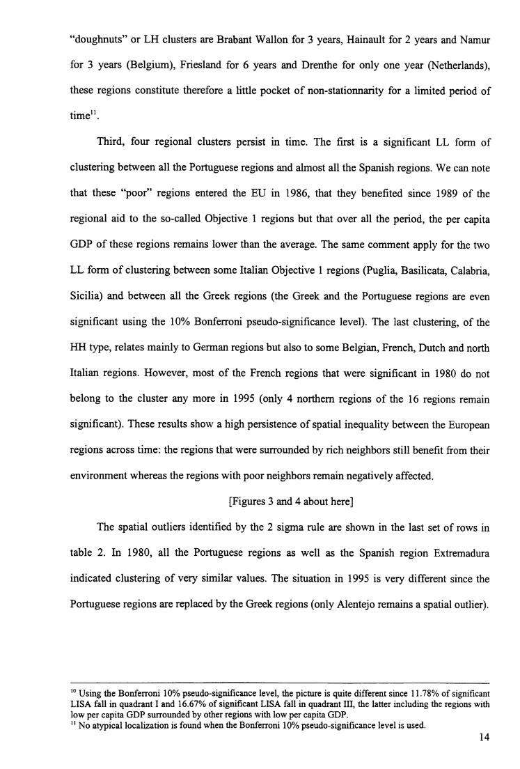
“doughnuts” or LH clusters are Brabant Wallon for 3 years, Hainault for 2 years and Namur
for 3 years (Belgium), Friesland for 6 years and Drenthe for only one year (Netherlands),
these regions constitute therefore a little pocket of non-stationnarity for a limited period of
time".
Third, four regional clusters persist in time. The first is a significant LL form of
clustering between all the Portuguese regions and almost all the Spanish regions. We can note
that these “poor” regions entered the EU in 1986, that they benefited since 1989 of the
regional aid to the so-called Objective 1 regions but that over all the period, the per capita
GDP of these regions remains lower than the average. The same comment apply for the two
LL form of clustering between some Italian Objective 1 regions (Puglia, Basilicata, Calabria,
Sicilia) and between all the Greek regions (the Greek and the Portuguese regions are even
significant using the 10% Bonferroni pseudo-significance level). The last clustering, of the
HH type, relates mainly to German regions but also to some Belgian, French, Dutch and north
Italian regions. However, most of the French regions that were significant in 1980 do not
belong to the cluster any more in 1995 (only 4 northern regions of the 16 regions remain
significant). These results show a high persistence of spatial inequality between the European
regions across time: the regions that were surrounded by rich neighbors still benefit from their
environment whereas the regions with poor neighbors remain negatively affected.
[Figures 3 and 4 about here]
The spatial outliers identified by the 2 sigma rule are shown in the last set of rows in
table 2. In 1980, all the Portuguese regions as well as the Spanish region Extremadura
indicated clustering of very similar values. The situation in 1995 is very different since the
Portuguese regions are replaced by the Greek regions (only Alentejo remains a spatial outlier).
10 Using the Bonferroni 10% pseudo-significance level, the picture is quite different since 11.78% of significant LISA fall in quadrant I and 16.67% of significant LISA fall in quadrant III, the latter including the regions with low per capita GDP surrounded by other regions with low per capita GDP.11 No atypical localization is found when the Bonferroni 10% pseudo-significance level is used.
14

3.4 Spatial patterns of growth rates
To refine this analysis, we apply the ESDA techniques to the growth rates of per capita
GDP in order to study the geographical patterns in growth processes.
The computation of Moran’s I statistics on the growth rate of per capita GDP between
1980 and 1995 of the various regions reveals a positive spatial autocorrelation (0.422 with a
/»-value of 0.0001). It means that the regions with relatively high per capita GDP growth rate
(respectively low) are localized close to other regions with relatively high per capita GDP
growth rate (respectively low) more often than if this localization was purely random.
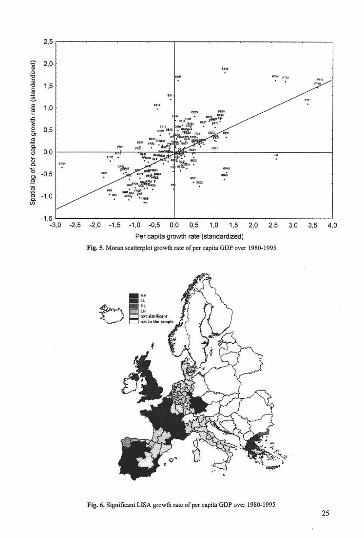
The Moran scatterplot for growth rates is displayed in figure 5. Compared to the
scatterplots for per capita GDP in 1980 and 1995, there is much more instability: only 73.2%
of the European regions show association of similar values (33.3% in quadrant I (HH) and
39.9% in quadrant III (LL)) while 26.8% of the regions are negatively associated (11.6% in
quadrant II (LH) and 15.2% in quadrant IV (HL)). All the Portuguese regions have growth
rates more than two standard deviations above the mean. Let’s recall that they were outliers in
the opposite quadrant in 1980. We will come back to this inverse relationship between the per
capita GDP in 1980 and growth rates at the end of this paragraph. Finally, the most extreme
observations according to the Moran regression diagnostics are shown in the last column of
table 2. As for per capita GDP in 1980 and 1995, there was no influential region according to
the Cook’s distance criterion.
[Figure 5 about here]
The procedure of evaluation of local spatial autocorrelation applied to the growth rates
(table 4, 3rd column) shows that the patterns of spatial association remain dominated by
clustering of LL or HH types12. Galicia and Asturias in Spain are the 2 regions with low
growth rates surrounded by regions with high growth rates. The regions with high growth
rates surrounded by regions with low growth rates are to be found in Greece : Anatoliki
Makedonia, Ionia Nisia and Kriti. The significant LISA at the 5% level are shown in figure 6.
15

To study the possible geographical characteristics implied by /? -convergence processes,
we compared the pattern of spatial association of growth rate with the pattern of spatial
association of initial per capita GDP (table 4, first and 3rd columns) in order to look for a
possible inverse relationship. Several results can be underlined.
It appears that, in only 43% of the cases, the regions that were in a certain quadrant for
per capita GDP level in 1980 are in the opposite quadrant for their growth rate. But this global
feature masks different behaviors. Thus, the regions of Portugal and some Spanish regions had
in 1980 a low per capita GDP and were surrounded by regions with low per capita GDP
(clustering of the LL type) but their growth rate is, as for their neighbors, higher than the
average (clustering of the HH type). The spatial autocorrelation indicators highlight the
dynamic character of these regions, whose economic performances within the group of the
Southern regions of Europe were often underlined. On the contrary, the majority of the French
regions, the British regions, some regions in Belgium and in the Netherlands, are
characterized by a configuration of the initial per capita GDP of HH type and a configuration
of the growth rates of the LL type.
Other characteristics between the patterns of spatial association can be highlighted. On
the one hand, within the group of the Southern regions, certain poor regions of Spain, Italy
and Greece do not manage to take off, just like their neighbors (configurations of the LL type
for the initial per capita GDP and the growth rates) or in spite of the dynamism of their
neighbors (configuration of the LL type for the initial per capita GDP and of LH type for the
growth rates). These regions thus show strong signs of delay of development. On the other
hand, almost all the German regions are very dynamic since they started with high levels, as
well as their neighbors and still had a HH type form of clustering for their growth rates.
[Table 4 about here]
[Figure 6 about here]
12 42.7% (15.2%) of the LISA computed are significant at the 5% pseudo-level (resp. 10% Bonferroni pseudolevel).
16

4 Conclusion
The study of the spatial distribution of regional per capita GDP in Europe over 1980-
1995 using Exploratory Spatial Data Analysis (ESDA) highlights the importance of spatial
interactions and geographical locations in regional growth and convergence issues. ESDA
appears therefore as a powerful tool to finely reveal the characteristics of economic
development of each region in relation to those of its geographical environment.
First, ESDA reveals significant positive global spatial autocorrelation, which is
persistent over the whole period: regions with relatively high (resp. low) per capita GDP are
and remain localized close to other regions with relatively high (low) per capita GDP and that
the spatial distribution of regional per capita GDP is not random. From the applied
econometrics perspective, this result has a major implication for the suitable estimation of
/^-convergence models: spatial autocorrelation should systematically be tested for in cross
section specifications and if detected, an appropriate spatial specification (spatial
autoregressive model, spatial error model or spatial cross regressive model) should be
estimated using the proper econometric tools to achieve reliable statistical inference.
Second, the Moran scatterplot and LISA show the persistence of the high-high and low-
low clustering types for regional per capita GDP, confirming the north-south polarization of
European regions. This reveals some kind of spatial heterogeneity hidden in the global
positive spatial autocorrelation pattern and may indicate the co-existence of two distinct
spatial regimes. Spatial effects could then perform differently in Northern Europe than in
Southern Europe. Moreover the convergence process, if it exists, may be different across
regimes. Once again from the applied econometrics perspective, this result suggest that the
potential for distinct spatial regimes should also be considered carefully in the estimation of
/^-convergence models, which should be tested for structural instability. All these aspects will
be studied in further research.
17

References
Abraham F, Von Rompuy P (1995) Regional convergence in the European Monetary Union. Papers in Regional Science 74: 125-142
Anselin L (1995) Local indicators of spatial association-LISA. Geographical Analysis 27: 93-115 Anselin L (1996) The Moran scatterplot as an ESDA tool to assess local instability in spatial
association. In: Fisher M, Schölten HJ, Unwin D (eds) Spatial analytical perspectives on GIS. Taylor & Francis, London
Anselin L (1998a) Interactive techniques and exploratory spatial data analysis. In: Longley PA, Goodchild MF, Maguire DJ, Wind DW (eds) Geographical information systems: principles, techniques, management and applications. Wiley, New York
Anselin L (1998b) Exploratory spatial data analysis in a geocomputational environment. In: Longley PA, Brooks SM, McDonnell R, Macmillan B (eds) Geocomputation, a primer. Wiley, New York
Anselin L (1999) SpaceStat, a software package for the analysis of spatial data, Version 1.90. Ann Arbor, BioMedware
Anselin L (2000) Spatial econometrics. In: Baltagi B (eds) Companion to econometrics. Basil Blackwell, Oxford.
Armstrong H (1995) Convergence among the regions of the European union. Papers in Regional Science 74: 143-152
Bailey T, Gatrell AC (1995) Interactive spatial data analysis. Harlow, Longman Belsley D, Kuh E, Welsch R (1980) Regression diagnostics: identifying influential data and sources
of collinearity. Wiley, New York Cliff AD, Ord JK (1973) Spatial autocorrelation. London, Pion Cliff AD, Ord JK (1981) Spatial processes: models and applications. London, Pion Cook R (1977) Detection of influential observations in linear regression. Technometrics 19: 15-18 Fingleton B (1999) Estimates of time to economic convergence: an analysis of regions of the
European Union. International Regional Science Review 22: 5-34 Getis A, Ord JK (1992) The analysis of spatial association by use of distance statistics. Geographical
Analysis 24: 189-206Haining R (1990) Spatial data analysis in the social and environmental sciences. Cambridge,
Cambridge University Press Haining R (1994) Diagnostics for regression modeling in spatial econometrics. Journal of Regional
Science 34: 325-341Haining R (1995) Data problems in spatial econometric modeling. In: Anselin L, Florax R (eds) New
directions in spatial econometrics. Springer, Berlin Hoaglin D, Welsch R (1978) The hat matrix in regression and ANOVA. The American Statistician 32:
17-22Löpez-Bazo E, Vayä E, Mora A, Surinach J (1999) Regional economic dynamics and convergence in
the European union. Annals of Regional Science 33: 343-370 Molle W, Boeckhout S (1995) Economic disparity under conditions of integration - A long term view
of the European case. Papers in Regional Science 74: 105-123 Neven D, Gouyette C (1995) Regional convergence in the European community. Journal of Common
Market Studies 33: 47-65Ord JK, Getis A, 1995, Local spatial autocorrelation statistics: distributional issues and an application.
Geographical Analysis 27: 286-305 Rey S (1999) Spatial empirics for economic growth and convergence, mimeo, San Diego State
University, SeptemberRey S, Montouri B (1999) US regional income convergence: a spatial econometric perspective.
Regional Studies 33: 143-1564 Savin NE (1984) Multiple hypotheses testing. In: Griliches Z, Intriligator MD (eds) Handbook of
Econometrics, volume II. Elsevier Science Publishers Sidäk Z (1967) Rectangular confidence regions for the means of multivariate normal distributions.
Journal of the American Statistical Assocation 62: 626-633 Upton GJG, Fingleton B (1985) Spatial data analysis by example. Wiley, New York Weisberg S (1985) Applied linear regression. Wiley, New York
18

Table 1. Moran’s / statistics for log per capita GDP over 1980-1995
Year Moran’s I Standard deviation Standardized value1980 0.774 0.033940 23.0241981 0.760 0.033971 22.5741982 0.746 0.033956 22.1611983 0.779 0.034083 23.0601984 0.757 0.034019 22.4461985 0.766 0.034077 22.6921986 0.785 0.034126 23.2131987 0.789 0.034164 23.2891988 0.773 0.034196 22.8021989 0.750 0.034221 22,1131990 0.762 0.034242 22.4611991 0.754 0.034311 22.1741992 0.770 0.034323 22.6511993 0.790 0.034272 23.2591994 0.799 0.034267 23.5141995 0.802 0.034222 23.653
Note: The expected value for Moran’s I statistic is constant for each year: E(l) = -0.007. All statistics are significant at p = 0.0001.
Table 2. Outliers : initial and terminal years and growth rates for log per capita GDP
1980 1995 GrowthRegion Studentized
ResidualRegion Studentized
ResidualRegion Studentized
ResidualSterea Ellada -3.445158 Ile de France -3.139385 Andalucia 3.497511
Bruxelles -2.893242 Hamburg -2.886250 Extremadura 2.822284Studentized Hamburg -2.500151 Bruxelles -2.654439 Galicia 2.745314
residuals Attiki -2.298205 Luxembourg (Lux) -2.612451 Luxembourg (Lux) -2.666020exceeding Ile de France -2.225954 Attiki -2.337432 Asturias 2.591420
2 in absolute Asturias -2.099516 Darmstadt -2.130149 Kriti -2.436728value Lüneburg 2.073019 Madrid -2.005542 Ionia Nisia
Notio Agaio-2.195220-2.142425
Region Leverage Region Leverage Region LeverageCentro 0.072428 Ipeiros 0.052553 Algarve 0.105763Norte 0.065610 Hamburg 0.046399 Centro 0.102492
Alentejo 0.062048 Voreio Aigaio 0.040424 Norte 0.089878Algarve 0.058095 Alentejo 0.038027 Sterea Ellada 0.065942
leverage Voreio Aigaio 0.038353 Darmstadt 0.037616 Lisboa 0.064531exceeding Hamburg 0.036314 Centro 0.034994 Luxembourg (Lux) 0.055558
4/N Extremadura 0.035489 Norte 0.032597 Alentejo 0.054656Ipeiros 0.035076 Dyptiki Ellada 0.031850 Picardie 0.030390
Bruxelles 0.032278 Oberbayem 0.031539Lisboa 0.031164 Luxembourg (Lux) 0.030974
Ionia Nisia 0.029664 Peloponnissos 0.030740Anatoliki Makedonia 0.029641 Bremen 0.029290
Region LISA Region LISA Region LISAExtremadura 3.668896 Anatoliki Makedonia 2.995502 Norte 3.708258
Norte 4.323912 Kentriki Makedonia 2.587855 Centro 5.333233Centro 5.100167 Dyptiki Makedonia 2.769021 Lisboa 4.516306
LISA Lisboa 3.432059 Thessalia 2.891856 Alentejo 4.173558outliers Alentejo 4.938435 Ipeiros 3.841003 Algarve 5.762157
(2-sigma Algarve 4.744208 Ionia Nisia 2.69785rule) Dyptiki Ellada
Sterea Ellada Peloponnisos Voreio Aigaio
Alentejo
3.1088092.6638723.0454413.2755642.801488
19

•o<DNECDTJC3Q.oCDro'a.cook_<DQ.O)O
03
CDCLCO
Log per capita GDP (standardized)
Fig. 1. Moran scatterplot for log per capita GDP 1980
Fig. 2. Moran scatterplot log per capita GDP 1995
2 0

Table 3. Local Indicators of Spatial Association (LISA): Log per capita GDP (1980-1995)
Code Region Signif HH LH LL HL Years 5% Years 10% Bonf.BELGIUM
Be1 Bruxelles 1(0) 1 80Be21 Anvers 6(0) 6 80-81 ;87; 93-95Be22 Limburg (B) 12(0) 12 80-83;85-88;92-95Be23 Oost Vlaanderen 4(0) 4 80-81:94-95Be24 Vlaams Brabant 4(0) 4 80-81;94-95Be25 West Vlaanderen 5(0) 5 80-81:93-95Be31 Brabant Wallon 5(0) 2 3 80:95/81:93-94Be32 Hainaut 4(0) 2 2 80-81 / 94-95Be33 Liège 4(0) 4 80:93-95Be34 Luxembourg (B) 9(0) 9 80-81:86-88:92-95Be35 Namur
GERMANY5(0) 2 3 80-81 / 93-95
De11 Stuttgart 16(15) 16(15) 80-95 80:82-95Del 2 Karlsruhe 16(16) 16(16) 80-95 80-95Del 3 Freiburg 16(16) 16(16) 80-95 80-95De14 Tübingen 16(16) 16(16) 80-95 80-95De21 Oberbayem 16(9) 16(9) 80-95 83-84:87-88:91-95De22 Niederbayem 16(9) 16(9) 80-95 87-95De23 Oberpfalz 16(16) 16(16) 80-95 80-95De24 Oberfranken 16(13) 16(13) 80-95 83-95De25 Mittelfranken 16(15) 16(15) 80-95 80:82-95De26 Unterfranken 16(13) 16(13) 80-95 83-95De27 Schwaben 16(13) 16(13) 80-95 83-95De5 Bremen 16(0) 16 80-95De6 Hamburg 16(3) 16(3) 80-95 93-95De71 Darmstadt 16(2) 16(2) 80-95 93:95De72 Giessen 16(11) 16(11) 80-95 80:83-84:86-88:91-95De73 Kassel 16(4) 16(4) 80-95 92-95De91 Braunschweig 16(11) 16(11) 80-95 80:82-84:87-88:91-95De92 Hannover 16(7) 16(7) 80-95 80:82-84:93-95De93 Lüneburg 16(14) 16(14) 80-95 80-88:91-95De94 Weser-Ems 16(5) 16(5) 80-95 80-83:95Deal Düsseldorf 14(0) 14 80-90:93-95Dea2 Köln 14(0) 14 80-81:83:85-95Dea3 Münster 16(0) 16 80-95Dea4 Detmold 16(2) 16(2) 80-95 93:95Dea5 Arnsberg 16(3) 16(3) 80-95 93-95Deb1 Koblenz 16(3) 16(3) 80-95 93-95Deb2 Trier 12(0) 12 80-81:85-90:92-95Deb3 Rheinhessen-Pfalz 16(16) 16(16) 80-95 80-95Dec Saarland 16(0) 16 80-95Def Schleswig-Holstein 16(10) 16(10) 80-95 81-87:93-95Dk DENMARK
SPAIN16(7) 16(7) 80-95 80:82-84:93-95
Es11 Galicia 16(15) 16(15) 80-95 80-91:93-95Es12 Asturias 16(10) 16(10) 80-95 80-88:94Es13 Cantabria 16(0) 16 80-95Es21 Pais Vasco 9(0) 9 81-87 :94-95Es22 Navarra 7(0) 7 81-87Es23 La Rioja 11(0) 11 80-88:94-95Es24 Aragon 4(0) 4 82-85Es3 Madrid 16(7) 14(7) 2 80-90:93-95/91-92 81-87Es41 Castilla-Leon 16(5) 16(5) 80-95 81-85Es42 Castilla-la Mancha 16(2) 16(2) 80-95 82-83Es43 Extremadura 16(16) 16(16) 80-95 80-95Es51 Cataluña 0(0)Es52 Valenciana 13(0) 13 80-89:93-95Es53 Islas Baleares 9(0) 9 80-86:94-95Es61 Andalucía 16(16) 16(16) 80-95 80-95Es62 Murcia
FRANCE16(5) 16(5) 80-95 81-85
Fr1 Ile de France 2(0) 2 80-81Fr21 Champagne-Ardenne 9(0) 9 80-82 ;85-87 :93-95Fr22 Picardie 10(0) 10 80-83:85-87:93-95Fr23 Haute-Normandie 10(0) 10 80-89Fr24 Centre 8(0) 8 80-87Fr25 Basse-Normandie 10(0) 10 80-89Fr26 Bourgogne 11(1) 11(1) 80-90 81Fr3 Nord-Pas-De-Calais 3(0) 3 80-81:95Fr41 Lorraine 16(0) 16 80-95Fr42 Alsace 16(2) 16(2) 80-95 80:95Fr43 Franche-Comté 16(0) 16 80-95Fr51 Pays de la Loire 8(0) 8 80-87Fr52 Bretagne 10(0) 10 80-89Fr53 Poitou-Charentes 8(0) 8 80-87Fr61 Aquitaine 0(0)Fr62 Midi-Pyrénées 0(0)
21
Code Region HH LH LL HL Years 5% Years 10% Bonf.Fr63 Limousin 9(0) 9 80-88Fr71 Rhöne-Alpes 2(0) 2 86-87Fr72 Auvergne 4(0) 4 80-82 ;86Fr81 Languedoc-Roussillon 0(0)Fr82 PACA
GREECE9(0) 9 83-91
Gr11 Anatoliki Makedonia 16(16) 16(16) 80-95 80-95Gr12 Kentriki Makedonia 16(16) 16(16) 80-95 80-95Gr13 Dytiki Makedonia 16(16) 16(16) 80-95 80-95Gr14 Thessalia 16(16) 16(16) 80-95 80-95Gr21 Ipeiros 16(16) 16(16) 80-95 80-95Gr22 Ionia Nisia 16(16) 16(16) 80-95 80-95Gr23 Dytiki Ellada 16(16) 16(16) 80-95 80-95Gr24 Sterea Ellada 16(16) 16(16) 80-95 80-95Gr25 Peloponnisos 16(16) 16(16) 80-95 80-95Gr3 Attiki 16(16) 16(16) 80-95 80-95Gr41 Voreio Aigaio 16(16) 16(16) 80-95 80-95Gr42 Notio Aigaio 16(16) 16(16) 80-95 80-95Gr43 Kriti
ITALY16(16) 16(16) 80-95 80-95
It11 Piemonte 14(0) 14 81-94It12 Valle d'Aosta 16(0) 16 80-95It13 Liguria 10(0) 10 83-92It2 Lombardia 12(3) 12(3) 83-94 89-91It31 Trentino - Alto Adige 15(2) 15(2) 81-95 90-91It32 Veneto 12(1) 12(1) 83-94 91It33 Friuli - Venezia Giulia 14(1) 14(1) 82-95 91It4 Emilia - Romagna 9(0) 9 84-92It51 Toscana 7(0) 7 86-92It 52 Umbria 0(0)It53 Marche 0(0)It6 Lazio 0(0)It71 Abruzzo 0(0)It72 Molise 1 (0) 1 95It8 Campania 4(0) 4 80-82;95It91 Puglia 16(2) 16(2) 80-95 94-95It92 Basilacata 6(0) 6 80-82;93-95It93 Calabria 16(2) 16(2) 80-95 94-95Ita Sicilia 8(0) 8 80-83:85:93-95Itb Sardegna 0(0)Lu LUXEMBOURG
NEDERLAND7(0) 7 80-81:86-87:93-95
NI12 Friesland 16(0) 10 6 80-87:93-95 / 85:88-92Nil 3 Drenthe 16(1) 15(1) 1 80-91:93-95/92 80NI2 Oost Nederland 12(0) 12 80-88:93-95NI31 Utrecht 14(0) 14 80-90:93-95NI32 Noord-Holland 12(0) 12 80-88:93-95NI33 Zuid-Holland 5(0) 5 80-81:93-95NI34 Zeeland 5(0) 5 80-81:93-95NI41 Noord-Brabant 12(0) 12 80-83:86-90:93-95NI42 Limburg (NL)
PORTUGAL6(0) 6 80-81:87 :93-95
Pt11 Norte 16(16) 16(16) 80-95 80-95Pt12 Centro 16(16) 16(16) 80-95 80-95Pt13 Lisboa e vale do Tejo 16(16) 16(16) 80-95 80-95Pt14 Alentejo 16(16) 16(16) 80-95 80-95Pt15 Algarve
UNITED-KINGDOM16(16) 16(16) 80-95 80-95
Uk1 North 0(0)Uk2 Yorkshire and Humberside 0(0)Uk3 East Midlands 0(0)Uk4 East Anglia 1 (0) 1 81Uk5 South East 0(0)Uk6 South West 0(0)Uk7 West Midlands 0(0)Uk8 North West 0(0)Uk9 Wales 0(0)Uka Scotland 0(0)Ukb Northern Ireland 0(0)
Signif. tot. 5% 1459 908 15 534 2% versus total of 2208 66.08 41.12 0.68 24.18 0.09% versus signif. tot. 5% 62.23 1.03 36.6 0.14Signif. tot. 10% Bonf. (628) (260) (0) (368) (0)% versus total of 2208 28.44 11.78 0 16.67 0% versus signif. tot. 10% 41.4 0 58.6 0
Note: signif: number of years local statistics is significant at 5% pseudo-significance level (in brackets at 10% Bonferroni pseudo-significance level) based on 10000 permutations; HH, LH, LL and HL: number of years local statistics is respectively in quadrant I, II, III and IV of Moran’s scatterplot.
2 2

TABLE 4. Spatial Association Patterns: initial and terminal years and growth rates for log per capita GDP (1980-1995)
Code Region 1980 1995 growth
Be1BELGIUMBaixelles HH HH LL
Be21 Anvers HH HH LLBe22 Limburg (B) HH HH HLBe23 Oost Vlaanderen HH HH LLBe24 Vlaams Brabant HH HH HLBe25 West Vlaanderen HH HH HLBe31 Brabant wallon HH HH LLBe32 Hainaut HH LH LLBe33 Liège HH HH LHBe34 Luxembourg (B) HH HH HHBe35 Namur HH LH LH
De11GERMANYStuttgart HH* HH* HH
Del 2 Karlsruhe HH* HH* HHDel 3 Freiburg HH* HH* HLDe14 Tübingen HH* HH* HHDe21 Oberbayem HH HH* HHDe22 Niederbayem HH HH* HHDe23 Oberpfalz HH* HH* HHDe24 Oberfranken HH HH* HHDe25 Mittelfranken HH* HH* HHDe26 Unterfranken HH HH* HHDe27 Schwaben HH HH* HHDe5 Bremen HH HH HHDe6 Hamburg HH HH* HHDe71 Darmstadt HH HH* HHDe72 Giessen HH* HH* HHDe73 Kassel HH HH* HHDe91 Braunschweig HH* HH* HHDe92 Hannover HH* HH* HHDe93 Lüneburg HH* HH* HHDe94 Weser-Ems HH* HH* HLDeal Düsseldorf HH HH LLDea2 Köln HH HH HHDea3 Münster HH HH HLDea4 Detmold HH HH* HHDea5 Arnsberg HH HH* LHDeb1 Koblenz HH HH* HHDeb2 Trier HH HH HHDeb3 Rheinhessen-Pfalz HH* HH* LHDec Saarland HH HH HHDef Schleswig-Holstein HH HH* HHDk DENMARK HH* HH* HH
Es11SPAINGalicia LL* LL* LH*
Es12 Asturias LL* LL LHEs13 Cantabria LL LL LHEs21 Pais Vasco LL LL HHEs22 Navarra LL LL HHEs23 La Rioja LL LL HHEs24 Aragon LL LL HHEs3 Madrid LL LL HHEs41 Castilla-Leon LL LL HHEs42 Castillada Mancha LL LL HHEs43 Extremadura LL* LL* HH*Es51 Cataluña LL LL HLEs52 Valenciana LL LL HHEs53 Islas Baleares LL LL HHEs61 Andalucía LL*
ii-i HH*Es62 Murcia LL LL HH
Fr1FRANCEIle de France HH HH LL
Fr21 Champagne-Ardenne HH HH LLFr22 Picardie HH HH LLFr23 Haute-Normandie HH HH LLFr24 Centre HH HH LL*Fr25 Basse-Normandie HH HH LL*Fr26 Bourgogne HH HH LL*Fr3 Nord-Pas-De-Calais HH HH LLFr41 Lorraine HH HH LHFr42 Alsace HH* HH* LHFr43 Franche-Comté HH HH LL
Code Region 1980 1995 growthFr51 Pays de la Loire HH HH LLFr52 Bretagne HH HH LLFr53 Poitou-Charentes HH HH LLFr61 Aquitaine HL HL LLFr62 Midi-Pyr6n6es HH HL LLFr63 Limousin HH HH LLFr71 Rhöne-Alpes HH HH LLFr72 Auvergne HH HH LL*Fr81 Languedoc-Roussillon HH LH LLFr82 PACA
GREECEHH HH LL
Gr11 Anatoliki Makedonia LL* LL* HLGr12 Kentriki Makedonia LL* LL* LLGr13 Dytiki Makedonia LL* LL* LLGr14 Thessalia LL* LL* LLGr21 Ipeiros LL* LL* LLGr22 lonia Nisia LL* LL* HLGr23 Dytiki Ellada LL* LL* LLGr24 Sterea Ellada LL* LL* LLGr25 Peloponnisos LL* LL* LLGr3 Attiki LL* LL* LLGr41 Voreio Aigaio LL* LL* HLGr42 Notio Aigaio LL* LL* HLGr43 Kriti
ITALYLL* LL* HL
It11 Piemonte HH HH LLIt12 Valle d'Aosta HH HH LLIt13 Liguria HH HH HLIt2 Lombardia HH HH LHIt31 Trentino - Alto Adige HH HH HHIt 32 Veneto HH HH HHIt33 Friuli - Venezia Giulia HH HH HHIt4 Emilia - Romagna HH HH LHIt51 Toscana HH HH LHIt 52 Umbria LL LL LHIt53 Marche LL LL LHIt6 Lazio LL HL HLIt71 Abruzzo LL LL HLIt72 Molise LL LL HLIt8 Campania LL LL LLIt91 Puglia LL LL* LLIt92 Basilacata LL LL LHIt93 Calabria LL LL* HLIta Sicilia LL LL LHItb Sardegna LL LL HLLu LUXEMBOURG
NEDERLANDHH HH HL
NI12 Friesland HH HH LLNI13 Drenthe HH* HH LLNI2 Oost Nederland HH HH LLNI31 Utrecht HH HH HLNI32 Noord-Holland HH HH LLNI33 Zuid-Holland HH HH LLNI34 Zeeland HH HH LLNI41 Noord-Brabant HH HH HLNI42 Limburg (NL)
PORTUGALHH HH LL
Pt11 Norte LL* LL* HH*Pt12 Centro LL* LL* HH*Pt13 Lisboa e vale do Tejo LL* LL* HH*Pt14 Alentejo LL* LL* HH*R15 Algarve
UNITED-KINGDOMLL* LL* HH*
Uk1 North HH LL LL*Uk2 Yorkshire and Humberside HH LL LL*Uk3 East Midlands HH LL LL*Uk4 East Anglia HH LH LLUk5 South East HH HH LLUk6 South West HH LL LL*Uk7 West Midlands HH LL LL*Uk8 North West HH LL LL*Uk9 Wales LH LL LL*Uka Scotland HH LL LL*Ukb Northern Ireland LH LL LL*
Note: in bold significant at 5% (* significant at 10% Bonferroni) pseudo-signifiance level based on 10000 Permutations.
23

Fig. 3. Significant LISA Log per capita GDP 1980
Fig. 4. Significant LISA Log per capita GDP 1995
24
Spat
ial
lag
of pe
r ca
pita
grow
th
rate
(sta
ndar
dize
d)
- 3,0 - 2,5 - 2,0 - 1,5 - 1,0 - 0,5 0,0 0,5 1,0 1,5 2,0 2,5 3,0 3,5 4,0
Per capita growth rate (standardized)
Fig. 5. Moran scatterplot growth rate of per capita GDP over 1980-1995
Fig. 6. Significant LISA growth rate of per capita GDP over 1980-199525