Exploring Coupled Atmosphere‐Ocean Data Assimilation Strategies with an EnKF, a Low‐Order Model and CMIP5 data

Robert Tardif Gregory J. Hakim 

Chris Snyder

University of Washington

NCAR

L

World Weather Open Science Conference 2014, Montréal

Motivation

Growing interest in near‐term (interannual to interdecadal) climate predictions (Meehl et al. 2009, 2013)

2WWOSC 2014, Montréal

Boundary‐valueproblem

Need accurate external forcings: ‐ solar variability,‐ greenhouse gases,‐ aerosols, …

Model errorInitial‐valueproblem

Models drift away from obs. (large biases) =>‐ Improve models‐ Parameter estimation‐ Post‐processing (bias correction)‐ Anomaly initialization

Skill of uninitialized forecasts limited to large scale externally forced climate variability(Sakaguchi et al. 2012)

For accurate predictions of internal variability: need coherent initialization of coupled 

**low‐frequency** atmosphere & ocean

Challenges / overarching questions• Context: Interacting slow (ocean) & fast (atmosphere) components of 

the climate system

• Challenges & overarching questions:o Unclear how to best initialize the coupled system

Q1: Traditional NWP‐style data assimilation (DA) appropriate?

o Slow has the memory but fewer observations than in fast Q2: Possible to initialize poorly observed or unobserved ocean?

Can obs. info. be effectively transferred to key unobserved variablesacross atmosphere‐ocean interface? 

o Coherence between initial conditions of slow & fast relies on “cross‐media” covariances Q3: What do these look like? How to reliably estimate? 

Fast component is “noisy” (i.e. high‐frequencies)…

o Practical considerations  Q4: Can coupled DA be done at reasonable cost? 

3WWOSC 2014, Montréal

Initialization approaches• Various methods considered so far:

1. Forcing ocean model with atmospheric reanalyses: no ocean DA2. Data assimilation (DA) performed independently in atmosphere & 

ocean (i.e. combine independent atmospheric & oceanic reanalysis products)

3. Weakly coupled DA:  Assimilation done separately in atmosphere & ocean but use fully coupled model to “carry” information forward

4. Fully coupled DA: w/ cross‐media covariances, still in infancy (Zhang et al. 2007, 2010)

4

(simple)

(comprehensive)

Here, consider fully coupled ensemble DA

WWOSC 2014, Montréal

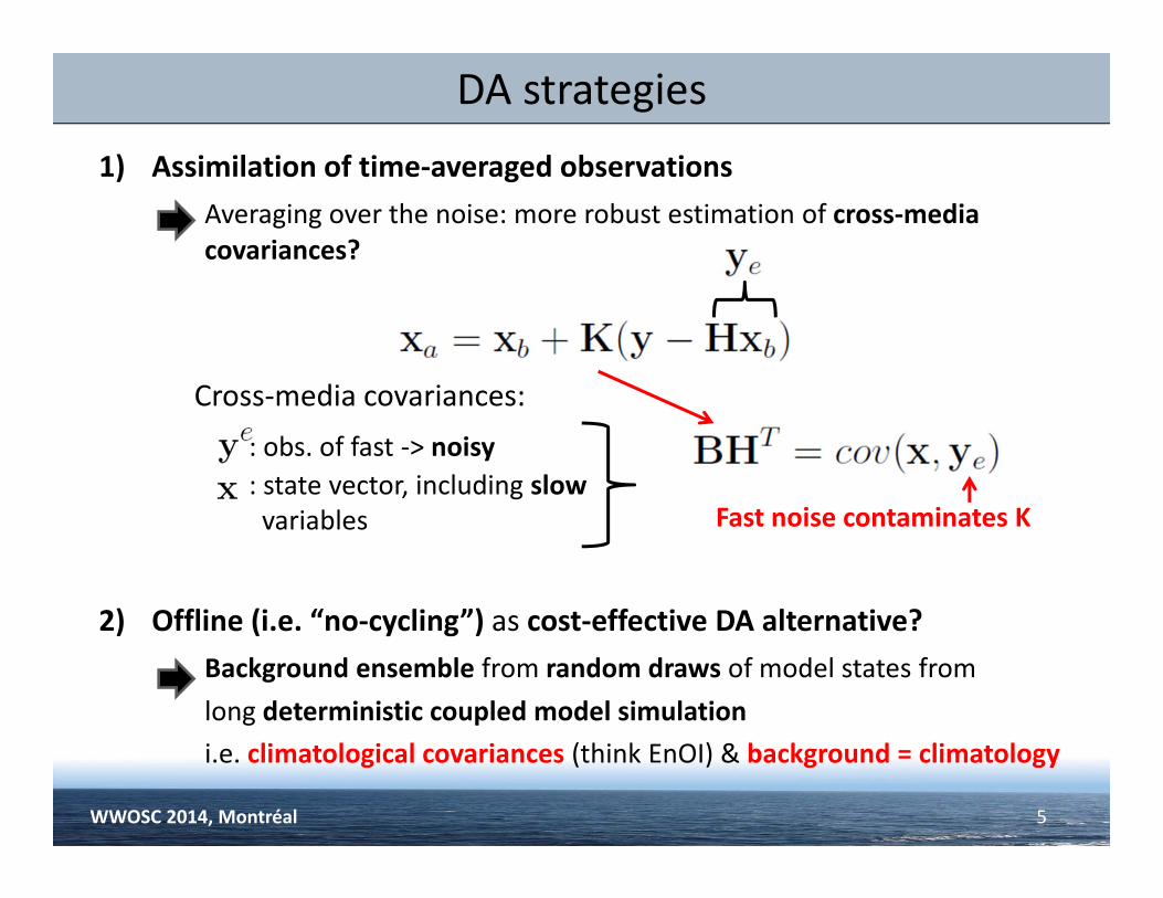
DA strategies1) Assimilation of time‐averaged observations

Averaging over the noise: more robust estimation of cross‐media covariances?

2) Offline (i.e. “no‐cycling”) as cost‐effective DA alternative?Background ensemble from random draws of model states from long deterministic coupled model simulationi.e. climatological covariances (think EnOI) & background = climatology

5

Cross‐media covariances: : obs. of fast ‐> noisy: state vector, including slowvariables Fast noise contaminates K

WWOSC 2014, Montréal

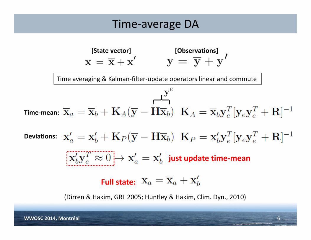
Time‐average DA

6

just update time‐mean

Time‐mean: 

Deviations:

(Dirren & Hakim, GRL 2005; Huntley & Hakim, Clim. Dyn., 2010)

Time averaging & Kalman‐filter‐update operators linear and commute

WWOSC 2014, Montréal

Full state:

[State vector] [Observations]

DA with simplified system• Use low‐order analogue of coupled North Atlantic climate system 

o Analyses of Atlantic meridional overtuning ciculation (AMOC) as canonical problem Key component in decadal/centennial climate variability & predictability

Not well observed (i.e. important challenge for coupled DA)

1. Low‐order coupled atmosphere‐ocean model Cheap to run: allows multiple realizations over the attractor

2. Promising concepts tested using data from a comprehensive AOGCM (i.e. CCSM4) To assess robustness of results in realistic system

7WWOSC 2014, Montréal

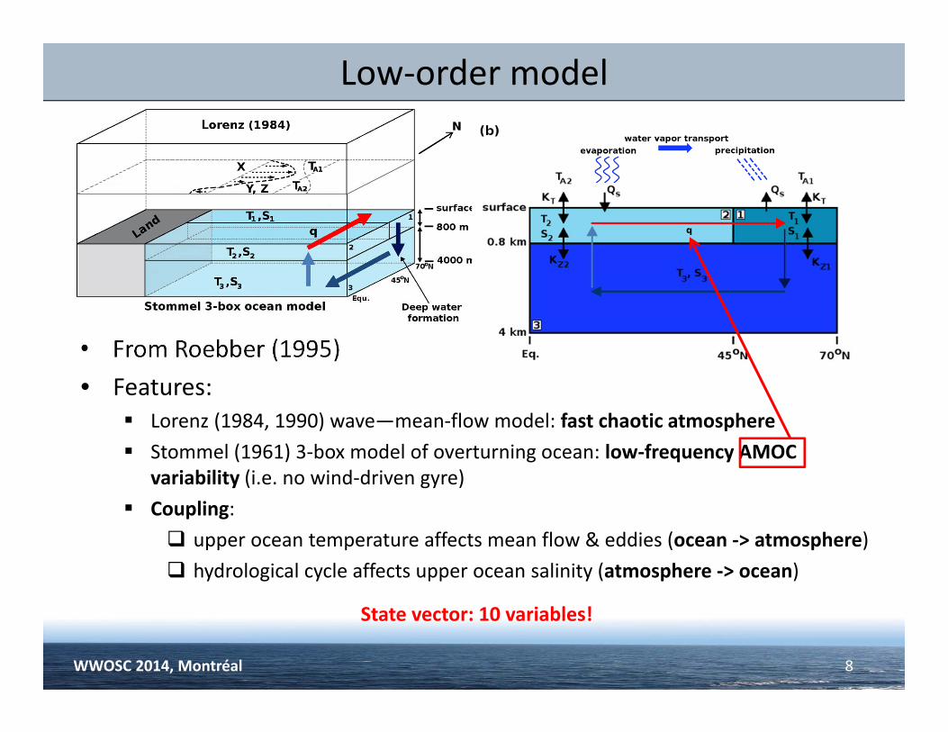
Low‐order model

• From Roebber (1995)• Features:

Lorenz (1984, 1990) wave—mean‐flow model: fast chaotic atmosphere Stommel (1961) 3‐box model of overturning ocean: low‐frequency AMOC 

variability (i.e. no wind‐driven gyre) Coupling: 

upper ocean temperature affects mean flow & eddies (ocean ‐> atmosphere) hydrological cycle affects upper ocean salinity (atmosphere ‐> ocean)

8

State vector: 10 variables!

WWOSC 2014, Montréal

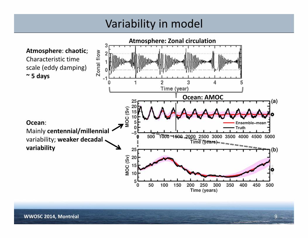
Variability in model

9

Ocean: AMOC

Atmosphere: Zonal circulation

Ocean: Mainly centennial/millennialvariability; weaker decadal variability

Atmosphere: chaotic;Characteristic time scale (eddy damping) ~ 5 days

WWOSC 2014, Montréal

Atmosphere—ocean covariability• Role of atmospheric observations in coupled DA

• Increase in covariability w.r.t. AMOC for annual & longer scales• Eddy “energy” (=X2+Y2) has more information than state variables 

(atmosphere ‐> ocean coupling through hydrologic cycle)

10

Correlations with AMOC vs averaging time

day

yearXYZ

WWOSC 2014, Montréal

DA experiments• EnKF w/ perturbed obs. & inflation for calibrated ensembles• Perfect model framework: (obs. from “truth” w/ Gaussian noise added)• Obs. error stats: large SNR (to mimmick “reliable” modern obs). • 100‐member ensemble

• Compared: o daily DA (availability of observations) » frequent assimilation of 

raw observations (i.e. NWP‐style DA)o time‐averaged DA (annual cycling)

o Data denial: from well‐observed ocean (except AMOC) to not observed at all (atmospheric obs. only)

o Cycling vs. “no‐cycling”

11WWOSC 2014, Montréal

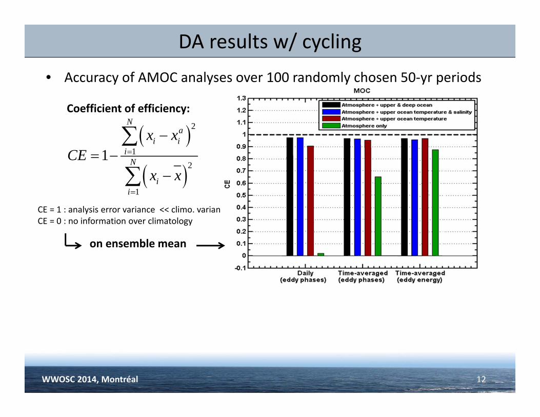
DA results w/ cycling

12

2

12

1

1

Na

i ii

N

ii

x xCE

x x

Coefficient of efficiency: 

• Accuracy of AMOC analyses over 100 randomly chosen 50‐yr periods

CE = 1 : analysis error variance  << climo. varianceCE = 0 : no information over climatology

WWOSC 2014, Montréal

on ensemble mean

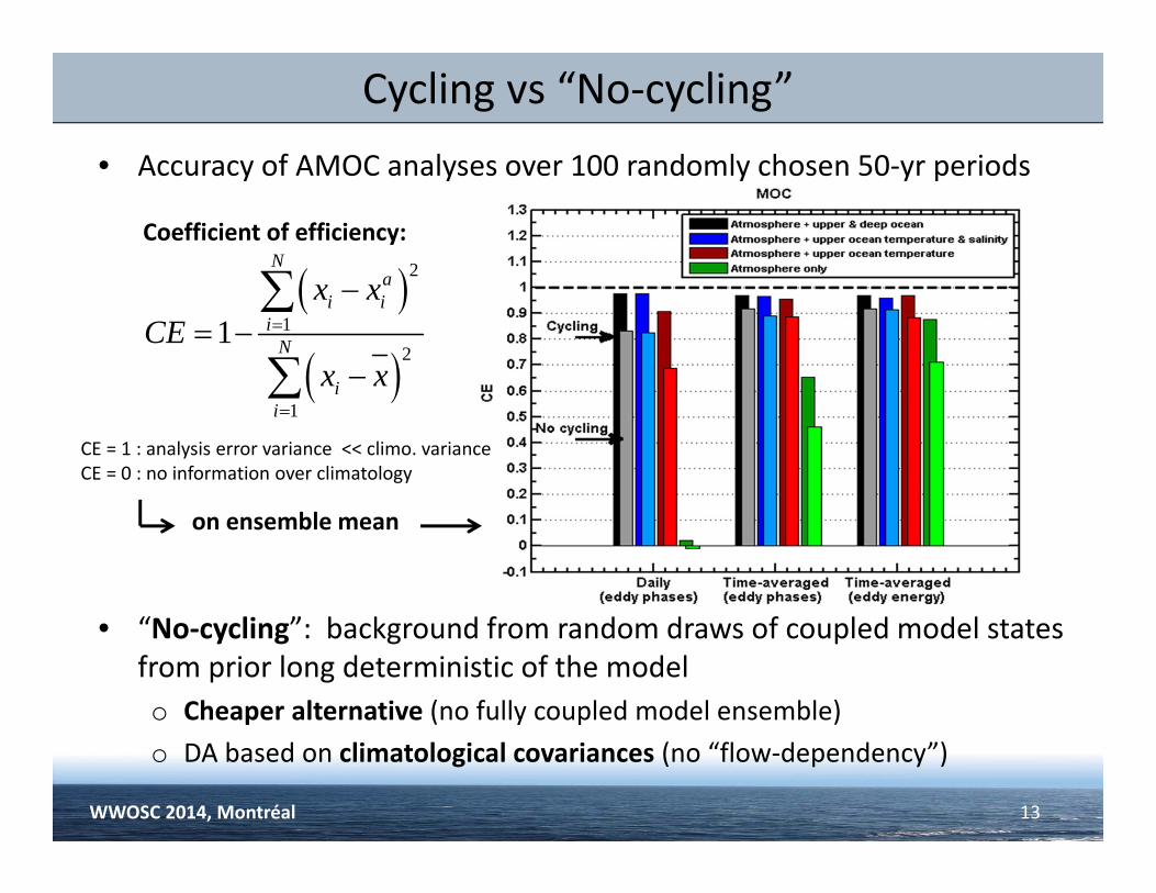
Cycling vs “No‐cycling”

13

2

12

1

1

Na

i ii

N

ii

x xCE

x x

Coefficient of efficiency: 

• Accuracy of AMOC analyses over 100 randomly chosen 50‐yr periods

• “No‐cycling”:  background from random draws of coupled model states from prior long deterministic of the modelo Cheaper alternative (no fully coupled model ensemble)o DA based on climatological covariances (no “flow‐dependency”)

CE = 1 : analysis error variance  << climo. varianceCE = 0 : no information over climatology

WWOSC 2014, Montréal

on ensemble mean

“No‐cycling” DA w/ comprehensive AOGCM• Strategy: derive low‐order analogue using CCSM4 gridded output

o “Coarse‐grained” representation of the N. Atlantic climate system, but underlying complex (i.e. realistic) dynamics

o 1000‐yr “Last Millenium” CMIP5 simulation (pre‐industrial natural variability)o Low‐order variables: Ocean: T & S averaged over boxes [ upper (i.e. 200m) subpolar ocean ] Atmosphere: Eddy heat flux across 40oN & MSLP along transect at 40oN  AMOC index: Max. value of overturning streamfunction in N. Atlantic

14

monthly

10‐yr running mean

WWOSC 2014, Montréal

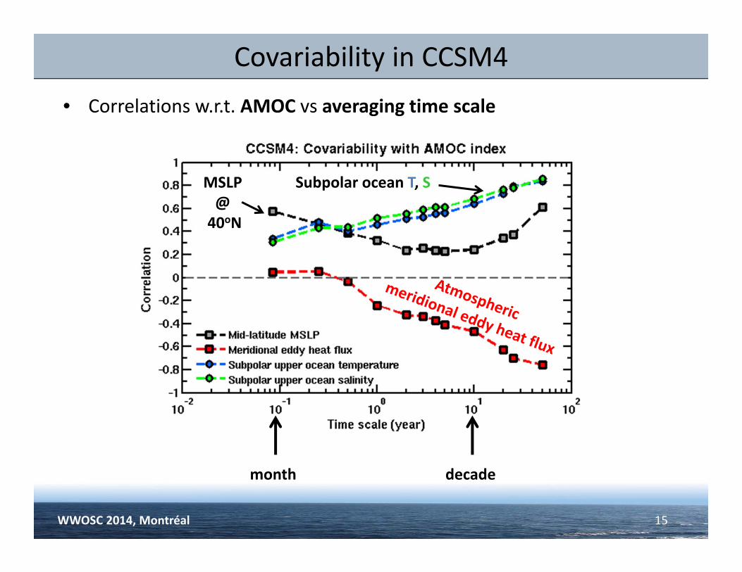
Covariability in CCSM4• Correlations w.r.t. AMOC vs averaging time scale

15WWOSC 2014, Montréal

Subpolar ocean T, S

month decade

MSLP @ 40oN

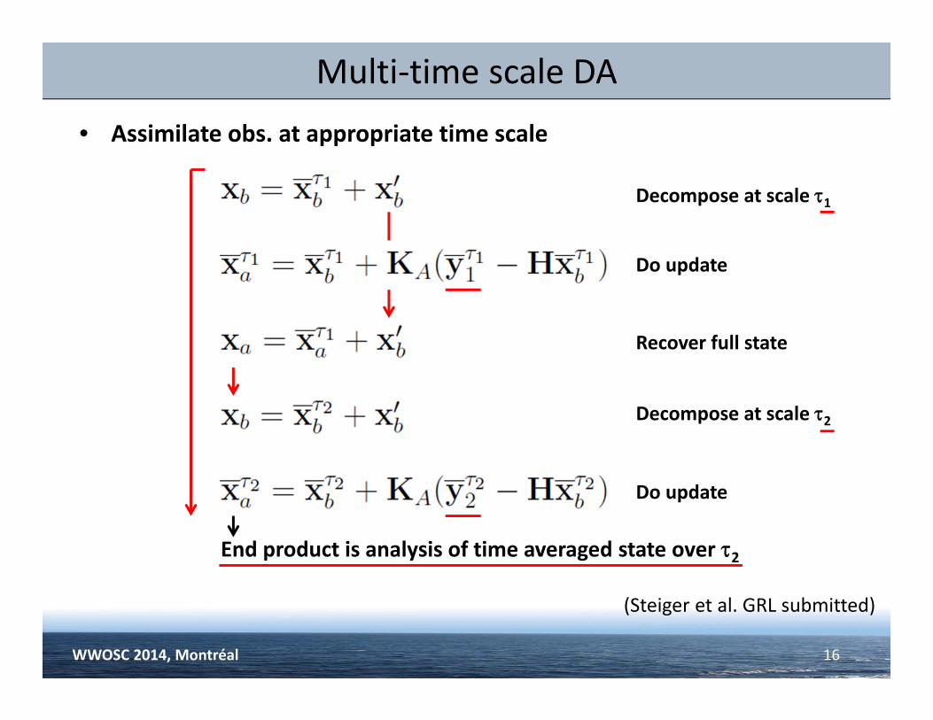
Multi‐time scale DA• Assimilate obs. at appropriate time scale

16

(Steiger et al. GRL submitted)

WWOSC 2014, Montréal

End product is analysis of time averaged state over 2 

Recover full state

Do update

Decompose at scale 1

Do update

Decompose at scale 2

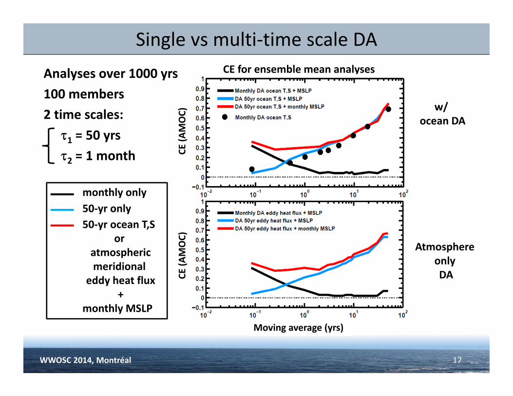
Analyses over 1000 yrs100 members2 time scales:

1 = 50 yrs2 = 1 month

Single vs multi‐time scale DA

17WWOSC 2014, Montréal

w/ ocean DA

Atmosphere only DA

CE for ensemble mean analyses

monthly only50‐yr only50‐yr ocean T,S

or atmosphericmeridional

eddy heat flux+

monthly MSLP

Moving average (yrs)

Moving average (yrs)

CE (A

MOC)

CE (A

MOC)

Summary & conclusions• Q1: NWP‐style DA appropriate to initialize slow component?

A: Yes, if *sufficient* obs. in ocean• Q2: Possible to initialize poorly observed or unobserved ocean? 

(i.e. ocean DA vs fully coupled DA)A: Yes, with time‐average DAo Frequent ocean DA slightly more effective when ocean is well‐observedo Fully coupled DA of time‐averaged obs. critical with poorly observed 

ocean• Q3: How to reliably estimate cross‐media covariances?

A: Use time‐averaging over appropriate scaleo Averaging over “noise” in fast component = > enhanced covariability

• Q4: Simplified cost‐effective coupled DA available?A: Yes, “no‐cycling” DA (of time‐averaged obs.) cheap & viable  

alternative

18WWOSC 2014, Montréal