1

Exploring Structural Consistency in GraphRegularized Joint Spectral-Spatial Sparse Coding

for Hyperspectral Image ClassificationChanghong Liu, Jun Zhou, Senior Member, IEEE, Jie Liang, Yuntao Qian, Member, IEEE, Hanxi Li,

and Yongsheng Gao, Senior Member, IEEE

Abstract—In hyperspectral image classification, both spec-tral and spatial data distributions are important in describingand identifying different materials and objects in the image.Furthermore, consistent spatial structures across bands can beuseful in capturing inherent structural information of objects.These imply that three properties should be considered whenreconstructing an image using sparse coding methods. Firstly,the distribution of different ground objects leads to differentcoding coefficients across the spatial locations. Secondly, localspatial structures change slightly across bands due to differentreflectance properties of various object materials. Lastly andmore importantly, some sort of structural consistency shall beenforced across bands to reflect the fact that the same objectappears at the same spatial location in all bands of an image.Based on these considerations, we propose a novel joint spectral-spatial sparse coding model that explores structural consistencyfor hyperspectral image classification. For each band image, weadopt a sparse coding step to reconstruct the structures in theband image. This allows different dictionaries be generated tocharacterize the band-wise image variation. At the same time,we enforce the same coding coefficients at the same spatiallocation in different bands so as to maintain consistent structuresacross bands. To further promote the discriminating power ofthe model, we incorporate a graph Laplacian sparsity constraintinto the model to ensure spectral consistency in the dictionarygeneration step. Experimental results show that the proposedmethod outperforms some state-of-the-art spectral-spatial sparsecoding methods.

Index Terms—Hyperspectral image, structural consistency,sparse coding, graph Laplacian regularizer.

I. INTRODUCTION

Remote sensing hyperspectral images (HSI) are acquiredin hundreds of bands to measure the reflectance of earthsurface, discriminate various materials, and classify groundobjects. HSI classification aims at assigning each pixel with

C. Liu and H. Li are with the School of Computer and InformationEngineering, Jiangxi Normal University, Nanchang, 330022, China.

J. Zhou is with the School of Information and Communication Technol-ogy, Griffith University, Nathan, Australia. Corresponding author: J. Zhou(jun.zhou@griffith.edu.au)

J. Liang is with the School of Engineering, the Australian NationalUniversity, Canberra, Australia.

Y. Qian is with the Institute of Artificial Intelligence, College of ComputerScience, Zhejiang University, Hangzhou, 310027, China.

Y. Gao is with the School of Engineering, Griffith University, Nathan,Australia.

This work was supported by the Australian Research Council LinkageProject (No. LP150100658), the National Natural Science Foundation of China(No. 61571393, 61462042, 61365002, 61262036), and the Visiting ScholarsSpecial Funds from Young and Middle-aged Teachers Development Programfor Universities in Jiangxi Province.

one thematic class in a scene [1]. Various machine learningmodels have been proposed for this purpose, such as Bayesianmodel [1], random forest [2], neural networks [3], supportvector machines (SVM) [4]–[7], sparse representation [8]–[13], and deep learning [14], [15].

Many HSI classification methods make prediction based onthe spectral response at a single pixel [6], [8], [9], [16]–[19].While spectral information is essential in image classificationand material identification, information extracted from spatialdomain is very useful to discriminate various targets made ofthe same materials [20], [21]. To address this need, spectral-spatial HSI classification approaches have been reported, eachtype of approach exploring and exploiting different waysto integrate spatial features with spectral features. Mura etal. and Ghamisi et al. proposed mathematical morphologymethods to analyze spatial relationships between pixels usingstructured elements [22], [23]. Markov random field methodsconsidered spatial information by adding to the objectivefunction a term that defines spatial correlations in the priormodel [24], [25]. Qian et al. developed 3D discrete wavelettransform to extract 3D features along spectral and spatialdimensions simultaneously [26]. Moreover, many researchersproposed sparse representation methods to include spatialsparsity constraints or kernel function to integrate spectral andspatial features [10], [12], [27]–[31].

Among these approaches, sparse representation based clas-sifiers have achieved the state-of-the-art performance [27],[32]. They provide an effective way of modelling the spatialneighborhood relationship and the distribution of atoms in thespectral or spatial domain, so that both spectral and spatialinformation can be seamlessly integrated and modeled. Insparse representation, a test sample is treated as a linearcombination of atoms from training samples or a learneddictionary. A sparse regularization term is normally includedto learn a discriminative representation of images [33]–[35].Recently, structured sparsity priors are also incorporated intoreconstruction methods [12], [36]–[39]. These include jointsparsity constraint [40], group sparsity constrain [41], graphLaplacian sparsity constraint [36], low-rank constraint [42],and low-rank group sparsity constraint [12]. Graph Laplaciansparsity constraint is based on the spatial dependencies be-tween the neighboring pixels [12], [36]. It preserves the localmanifold structure so that if two data points are close in theiroriginal data space, the sparse representations of these twodata points are also close to each other in the new data space.

2

Band 6 Band 15 Band 32 Band 45 Band 80 Band 100

(a)

(b)

(c)

(d)

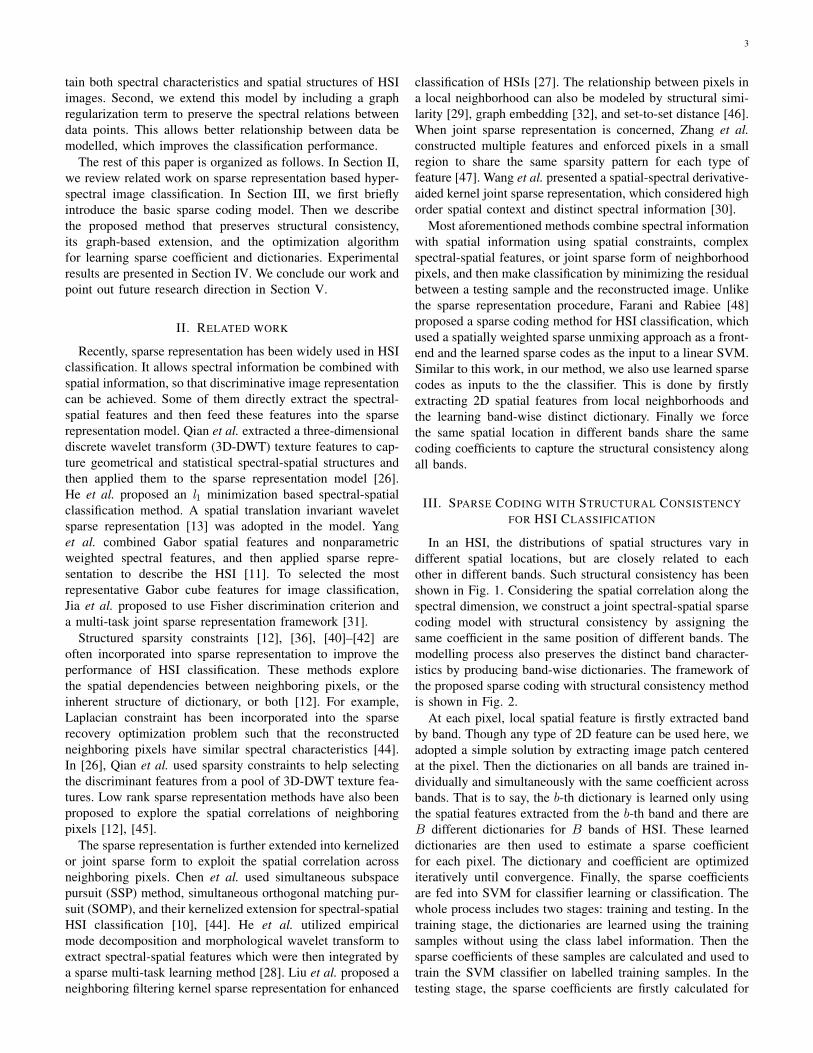
Fig. 1. Consistent structures in the University of Pavia dataset. (a) Pixel (362, 149) in bands 6, 15, 32, 45, 80 and 100 for the “Bitumen” class. (b) 13× 13patches centered at pixel (362, 149). (c) Pixel (251, 76) in bands 6, 15, 32, 45, 80 and 100 for the “Bricks” class. (d) 13× 13 patches centered at pixel (251,76).

Although spectral-spatial analysis has been studied inten-sively in HSI classification, how to explore the local structuralinformation has not been adequately addressed. To get a deeperunderstanding of the structural information embedded in ahyperspectral image, we use the University of Pavia imagein Fig. 1 as an example. In the first row, bands 6, 15, 32,45, 80 and 100 are displayed. In the second and fourth rows,small patches extracted from neighborhoods around pixels(362, 149) and (251, 76) are displayed, respectively. Threeobservations can be obtained from this figure. Firstly, variousland cover classes have different distributions in the spatialdomain. This happens in all bands. Secondly, local spatialstructures change slightly across different bands. This is dueto the distinct reflectance properties of object materials atdifferent light wavelength. As a consequence, the extractedGabor features at the same location in different bands alsochange slightly. Lastly and more importantly, some sort ofstructural consistency can be observed across bands, as theground objects at each location are consistent in all bands.Such consistency has been proved to be useful in hyperspec-tral image denoising [43]. In general, image representationand classification models shall be able to address all theseobservations.

Motivated by the above observations, we propose a noveljoint spectral-spatial framework to explore structural consis-tency along all bands in the sparse coding model. For eachband image, image patches or 2D image features centered atpixels are firstly extracted from local neighborhood, whichcontain local structures of the central pixels. Then a sparsecoding step is adopted to reconstruct the structures in theband images. This allows different dictionaries be generated tocharacterize the band-wise image variation. At the same time,consistent structures across bands are maintained by enforcingthe same coding coefficients at the same spatial location indifferent bands. To further promote the discriminating powerof the model, a graph Laplacian sparsity constraint is incor-porated into the model to ensure spectral consistency in thedictionary generation step. At last, the learned coefficients arefed into the classifier for pixel-wise classification.

The contribution of this paper lies in two aspects. First, wepropose a novel joint spectral-spatial sparse coding framework,which can explore the structural consistency along all bandsand integrate the spectral information and spatial structuresinto a sparse coding framework. Under this framework, 2Dstructural features can be applied to HSI classification effec-tively and directly, and the learned coefficients inherently con-

3

tain both spectral characteristics and spatial structures of HSIimages. Second, we extend this model by including a graphregularization term to preserve the spectral relations betweendata points. This allows better relationship between data bemodelled, which improves the classification performance.

The rest of this paper is organized as follows. In Section II,we review related work on sparse representation based hyper-spectral image classification. In Section III, we first brieflyintroduce the basic sparse coding model. Then we describethe proposed method that preserves structural consistency,its graph-based extension, and the optimization algorithmfor learning sparse coefficient and dictionaries. Experimentalresults are presented in Section IV. We conclude our work andpoint out future research direction in Section V.

II. RELATED WORK

Recently, sparse representation has been widely used in HSIclassification. It allows spectral information be combined withspatial information, so that discriminative image representationcan be achieved. Some of them directly extract the spectral-spatial features and then feed these features into the sparserepresentation model. Qian et al. extracted a three-dimensionaldiscrete wavelet transform (3D-DWT) texture features to cap-ture geometrical and statistical spectral-spatial structures andthen applied them to the sparse representation model [26].He et al. proposed an l1 minimization based spectral-spatialclassification method. A spatial translation invariant waveletsparse representation [13] was adopted in the model. Yanget al. combined Gabor spatial features and nonparametricweighted spectral features, and then applied sparse repre-sentation to describe the HSI [11]. To selected the mostrepresentative Gabor cube features for image classification,Jia et al. proposed to use Fisher discrimination criterion anda multi-task joint sparse representation framework [31].

Structured sparsity constraints [12], [36], [40]–[42] areoften incorporated into sparse representation to improve theperformance of HSI classification. These methods explorethe spatial dependencies between neighboring pixels, or theinherent structure of dictionary, or both [12]. For example,Laplacian constraint has been incorporated into the sparserecovery optimization problem such that the reconstructedneighboring pixels have similar spectral characteristics [44].In [26], Qian et al. used sparsity constraints to help selectingthe discriminant features from a pool of 3D-DWT texture fea-tures. Low rank sparse representation methods have also beenproposed to explore the spatial correlations of neighboringpixels [12], [45].

The sparse representation is further extended into kernelizedor joint sparse form to exploit the spatial correlation acrossneighboring pixels. Chen et al. used simultaneous subspacepursuit (SSP) method, simultaneous orthogonal matching pur-suit (SOMP), and their kernelized extension for spectral-spatialHSI classification [10], [44]. He et al. utilized empiricalmode decomposition and morphological wavelet transform toextract spectral-spatial features which were then integrated bya sparse multi-task learning method [28]. Liu et al. proposed aneighboring filtering kernel sparse representation for enhanced

classification of HSIs [27]. The relationship between pixels ina local neighborhood can also be modeled by structural simi-larity [29], graph embedding [32], and set-to-set distance [46].When joint sparse representation is concerned, Zhang et al.constructed multiple features and enforced pixels in a smallregion to share the same sparsity pattern for each type offeature [47]. Wang et al. presented a spatial-spectral derivative-aided kernel joint sparse representation, which considered highorder spatial context and distinct spectral information [30].

Most aforementioned methods combine spectral informationwith spatial information using spatial constraints, complexspectral-spatial features, or joint sparse form of neighborhoodpixels, and then make classification by minimizing the residualbetween a testing sample and the reconstructed image. Unlikethe sparse representation procedure, Farani and Rabiee [48]proposed a sparse coding method for HSI classification, whichused a spatially weighted sparse unmixing approach as a front-end and the learned sparse codes as the input to a linear SVM.Similar to this work, in our method, we also use learned sparsecodes as inputs to the the classifier. This is done by firstlyextracting 2D spatial features from local neighborhoods andthe learning band-wise distinct dictionary. Finally we forcethe same spatial location in different bands share the samecoding coefficients to capture the structural consistency alongall bands.

III. SPARSE CODING WITH STRUCTURAL CONSISTENCYFOR HSI CLASSIFICATION

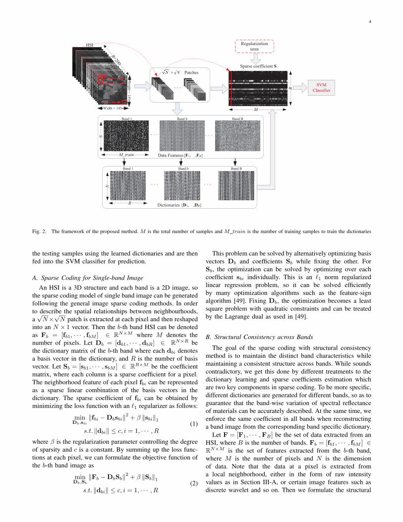
In an HSI, the distributions of spatial structures vary indifferent spatial locations, but are closely related to eachother in different bands. Such structural consistency has beenshown in Fig. 1. Considering the spatial correlation along thespectral dimension, we construct a joint spectral-spatial sparsecoding model with structural consistency by assigning thesame coefficient in the same position of different bands. Themodelling process also preserves the distinct band character-istics by producing band-wise dictionaries. The framework ofthe proposed sparse coding with structural consistency methodis shown in Fig. 2.

At each pixel, local spatial feature is firstly extracted bandby band. Though any type of 2D feature can be used here, weadopted a simple solution by extracting image patch centeredat the pixel. Then the dictionaries on all bands are trained in-dividually and simultaneously with the same coefficient acrossbands. That is to say, the b-th dictionary is learned only usingthe spatial features extracted from the b-th band and there areB different dictionaries for B bands of HSI. These learneddictionaries are then used to estimate a sparse coefficientfor each pixel. The dictionary and coefficient are optimizediteratively until convergence. Finally, the sparse coefficientsare fed into SVM for classifier learning or classification. Thewhole process includes two stages: training and testing. In thetraining stage, the dictionaries are learned using the trainingsamples without using the class label information. Then thesparse coefficients of these samples are calculated and used totrain the SVM classifier on labelled training samples. In thetesting stage, the sparse coefficients are firstly calculated for

4

B=200

× Patches

HSI

Dictionaries {D1, ,DB}

Sparse coefficient S

Band 1 Band b Band B

N

R

M

R

Width = 145

Heig

ht =

14

5

Data Features{F1, ,FB}

Band 1 Band b Band B

N

M_train

Regularization

term

SVM

Classifier

Fig. 2. The framework of the proposed method. M is the total number of samples and M train is the number of training samples to train the dictionaries

the testing samples using the learned dictionaries and are thenfed into the SVM classifier for prediction.

A. Sparse Coding for Single-band Image

An HSI is a 3D structure and each band is a 2D image, sothe sparse coding model of single band image can be generatedfollowing the general image sparse coding methods. In orderto describe the spatial relationships between neighbourhoods,a√N×√N patch is extracted at each pixel and then reshaped

into an N × 1 vector. Then the b-th band HSI can be denotedas Fb = [fb1, · · · , fbM ] ∈ RN×M where M denotes thenumber of pixels. Let Db = [db1, · · · ,dbR] ∈ RN×R bethe dictionary matrix of the b-th band where each dbi denotesa basis vector in the dictionary, and R is the number of basisvector. Let Sb = [sb1, · · · , sbM ] ∈ RR×M be the coefficientmatrix, where each column is a sparse coefficient for a pixel.The neighborhood feature of each pixel fbi can be representedas a sparse linear combination of the basis vectors in thedictionary. The sparse coefficient of fbi can be obtained byminimizing the loss function with an `1 regularizer as follows:

minDb,sbi

‖fbi −Dbsbi‖2 + β ‖sbi‖1

s.t. ‖dbi‖ ≤ c, i = 1, · · · , R(1)

where β is the regularization parameter controlling the degreeof sparsity and c is a constant. By summing up the loss func-tions at each pixel, we can formulate the objective function ofthe b-th band image as

minDb,Sb

‖Fb −DbSb‖2 + β ‖Sb‖1

s.t. ‖dbi‖ ≤ c, i = 1, · · · , R(2)

This problem can be solved by alternatively optimizing basisvectors Db and coefficients Sb while fixing the other. ForSb, the optimization can be solved by optimizing over eachcoefficient sbi individually. This is an `1 norm regularizedlinear regression problem, so it can be solved efficientlyby many optimization algorithms such as the feature-signalgorithm [49]. Fixing Db, the optimization becomes a leastsquare problem with quadratic constraints and can be treatedby the Lagrange dual as used in [49].

B. Structural Consistency across Bands

The goal of the sparse coding with structural consistencymethod is to maintain the distinct band characteristics whilemaintaining a consistent structure across bands. While soundscontradictory, we get this done by different treatments to thedictionary learning and sparse coefficients estimation whichare two key components in sparse coding. To be more specific,different dictionaries are generated for different bands, so as toguarantee that the band-wise variation of spectral reflectanceof materials can be accurately described. At the same time, weenforce the same coefficient in all bands when reconstructinga band image from the corresponding band specific dictionary.

Let F = [F1, · · · ,FB ] be the set of data extracted from anHSI, where B is the number of bands. Fb = [fb1, · · · , fbM ] ∈RN×M is the set of features extracted from the b-th band,where M is the number of pixels and N is the dimensionof data. Note that the data at a pixel is extracted froma local neighborhood, either in the form of raw intensityvalues as in Section III-A, or certain image features such asdiscrete wavelet and so on. Then we formulate the structural

5

consistency model for the whole HSI as

minD1,··· ,DB ,S

B∑b=1

‖Fb −DbS‖2 + β ‖S‖1

s.t. ‖dbi‖ ≤ c, i = 1, · · · , R, b = 1, · · · , B(3)

where D1, · · · ,DB ∈ RN×R are the dictionaries for differentbands, R is the size of dictionary, and S ∈ RR×M is thesparse coefficient matrix, which is the same for all bands.

C. Extension with Graph Constraint

In order to capture the structural relationship between theneighboring pixels and improve the discriminative capabilityof the learned model, sparse coding models are usually addedwith certain constraints [12], [36], [40]–[42]. In particular,recent work show that graph Laplacian sparsity constrainthas demonstrated exceptional performance when comparedwith alternatives [12]. Graph Laplacian sparsity constraints canpreserve the local manifold structure of data. If two data pointsxi and xj are close in their original space, the correspondingsparse coefficients si and sj shall also be close in the newspace.

Inspired by this idea, we also incorporate graph Laplaciansparsity constraint into the proposed method. This constraintbuilds the nearest neighbor graph using the spectral fea-ture. This makes the learned sparse coefficients preserve thematerial spectral characteristics and the spatial correlationsof pixels because local structures might be made of samematerials.

Let the spectral features of a set of pixels be X =[X1, · · · ,XM ] ∈ RB×M , where B is the number of bands,and M is the number of pixels. We construct a K-nearestneighbor (KNN) graph G with M vertices and calculatethe weight matrix W of G. If Xi is among the K-nearestneighbors of Xj or Xj is among the K-nearest neighbors ofXi, Wij = 1, otherwise, Wij = 0. The Laplacian constraintis to map the weighted graph G to the sparse coefficients S.It is defined as

Tr(SLST ) =1

2

M∑i=1

M∑j=1

(si − sj)Wij (4)

where L = P − W is the Laplacian matrix, P =diag(p1, · · · , pM ) is a diagonal matrix and pi =

∑Mj=1 Wij

is the degree of Xi. Combining the Laplacian constraint intothe sparse coding model in Equation (3), the objective func-tion of the graph-based sparse coding model with structuralconsistency is formulated as

minD1,··· ,DB ,S

B∑b=1

‖Fb −DbS‖2 + αTr(SLST ) + β ‖S‖1

s.t. ‖dbi‖ ≤ c, i = 1, · · · , R, b = 1, · · · , B.(5)

D. Iterative Optimization Process

The sparse coding problem is usually solved by the l1-normminimization optimization methods [36], [49]. Followed by

the l1-norm minimization, the problem in Equation (5) canbe solved by alternatively optimizing the dictionaries and thesparse coefficients while fixing the other. More specifically,the optimization procedure includes two iterative steps: (1)learning sparse coefficients S while fixing the dictionariesD1, · · · ,DB , and (2) learning the dictionaries D1, · · · ,DB

while fixing the sparse coefficients S.1) Learning Sparse Coefficients S: When fixing the dictio-

naries D1, · · · ,DB , the sparse coefficients S learning problembecomes

minS

B∑b=1

‖Fb −DbS‖2 + αTr(SLST ) + β ‖S‖1 . (6)

This can be rewritten as

minS

M∑i=1

B∑b=1

‖fib −Dbsi‖2 + α

M∑i,j=1

LijsTi sj + β

M∑i=1

‖si‖1

(7)where ‖si‖1 =

∑Rr=1 |s

(r)i | and s

(r)i is the r-th element of

si. Each vector si in S can be updated individually whilekeeping all the others vectors {sj}j 6=i as constants. Then theoptimization problem for si becomes

minsi

f(si) =

B∑b=1

‖fib −Dbsi‖2 +αLiisTi si + sTi hi + β ‖si‖1

(8)where

hi = 2α

∑j 6=i

Lijsj

(9)

Following the feature-sign search algorithm [49], the optimiza-tion problem in Equation (8) can be implemented by searchingfor the optimal active set, which is a set of potentially nonzerocoefficients, and their corresponding signs. The reasons aretwo-folds:

(1) If we know the signs of all elements in si, theoptimization problem in Equation (8) becomes a standardunconstrained quadratic optimization problem which can besolved analytically and efficiently.

(2) The non-smooth optimization theory [50] shows thatthe necessary condition for a parameter vector to be a localminima is that the zero-vector is an element of the sub-differential [36], so the active set A can be obtained by

A ={j|s(j)i = 0, |∇(j)

i gs(si)| > β}

(10)

where ∇(j)i denotes the subdifferentiable value of the jth

element of si, s(j)i is the jth element of si and gs(si) =∑B

b=1 ‖fib −Dbsi‖2 + αLiisTi si + sTi hi. For each iteration,

the j-th element with the largest sub-gradient value is selectedinto the active set from zero-value elements of si given by,

j = argmaxj|∇(j)

i gs(si)|. (11)

To locally improve this objective, the sign θj of s(j)i is

estimated by

θj =

{−1, if ∇(j)

i gs(si) > β

1, if ∇(j)i gs(si) < −β

(12)

6

Let θ be the signs corresponding to the active set A. Theoptimization problem in Equation (8) reduces to a standardunconstrained quadratic optimization problem

minsi

fnew (si) =

B∑b=1

∥∥∥fib − Dbsi

∥∥∥2 + αLiisTi si + sTi hi + βθ.

(13)This can be solved efficiently and the optimal value ofsi over the current active set can be obtained by letting(∂fnew (si)/∂si) = 0. Then we get

snewi = (

B∑b=1

DTb Db + αLiiI)

−1(

B∑b=1

DTb fbi − (hi + βθ)/2)

(14)where I is the identity matrix. Then the line search is per-formed between the current solution si and snewi to searchfor the optimal active set and signs which can minimize theobjective function in Equation (8) and get the optimal solutionmathbfs∗i . The algorithm for learning the sparse coefficientsS is summarized in Algorithm 1.

Algorithm 1 Learning sparse coefficients S based onfeature-sign searchInput:

Data from B bands F1, · · · ,FB ∈ RN×M .Dictionaries from B bands D1, · · · ,DB ∈ RN×R.Laplacian matrix L, regularization parameters β and α.

Output:The optimal coefficient matrix S = [s∗1, · · · , s∗M ].

1: for each i ∈ [1,M ] do2: initialize:3: si = ~0, θ = ~0 and the active set A = ∅.4: activate:5: Select j using Equation (11), activate s

(j)i (A = A ∪

{j}) and update the sign θj of s(j)i using Equation (12).6: feature-sign:7: Let D1, · · · , DB be the sub-matrices of D1, · · · ,DB

that contain only the columns corresponding to theactive set.

8: Let si, θ, and hi be the sub-vectors of si, θ, and hi

corresponding to the active set.9: Solve the unconstrained quadratic optimization problem

using Equation (13) and get the optimal value of si overthe current active set using Equation (14).

10: Perform a discrete line search on the closed line seg-ment from si to snewi and update si to the point withthe lowest objective value.

11: Remove the zero value of si from the active set andupdate θ = sign(si).

12: check the convergence conditions:13: (a) Convergence condition for nonzero coefficients:

∇(j)i gs(si) + βsign(s

(j)i ) = 0,∀s(j)i 6= 0. If condition

(a) is not satisfied, go to Step 6. Otherwise checkcondition (b).

14: (b) Covergence condition for zero coefficients:|∇(j)

i gs(si)| ≤ β. If condition (b) is not satisfied, go toStep 4, otherwise return si as the optimal solution s∗i .

15: end for

2) Learning dictionaries D1, · · · ,DB: In our method,different dictionaries are generated for different bands, butthese bands share the same sparse coefficients S for preservingconsistent structures in the image. The b-th dictionary isconstructed from data Fb in the b-th band, so the dictionaryin each band can be learned individually when fixing thesparse coefficients S. The problem of learning the dictionarybecomes a least squares problem with quadratic constraints foreach band, so the dictionaries D1, · · · ,DB can be obtainedseparately by the following objective function:

minD1

‖F1 −D1S‖2minD2

‖F2 −D2S‖2...

minDB

‖FB −DBS‖2

(15)

This optimization problem can be solved by the Lagrangiandual method. The whole procedure is summarized in Algo-rithm 2.

Algorithm 2 Optimizing dictionariesInput:

Data from B bands F1, · · · ,FB ∈ RN×Mtrain .Laplacian matrix Ltr ∈ RMtrain×Mtrain .Regularization parameters β and α. Iteration number ρand the objective error γ.

Output:Coefficient matrix Str ∈ RR×Mtrain .B bands of dictionaries D1, · · · ,DB ∈ RN×R.

1: Initialize B bands of dictionaries D1, · · · ,DB randomlyand set iteration counter t=1.

2: while (t ≤ ρ) do3: Update the coefficient matrix Str with Algorithm 1.4: Calculate the objective value Ot =∑B

b=1 ‖Fb −DbStr‖2 + αTr(StrLSTtr) + β ‖Str‖1

5: Update the dictionaries D1, · · · ,DB :6: for b = 1 to B do7: min

Db

‖Fb −DbStr‖28: end for9: if (Ot−1 −Ot) < γ then

10: break11: end if12: t← t+ 113: end while

E. Discussion and Analysis

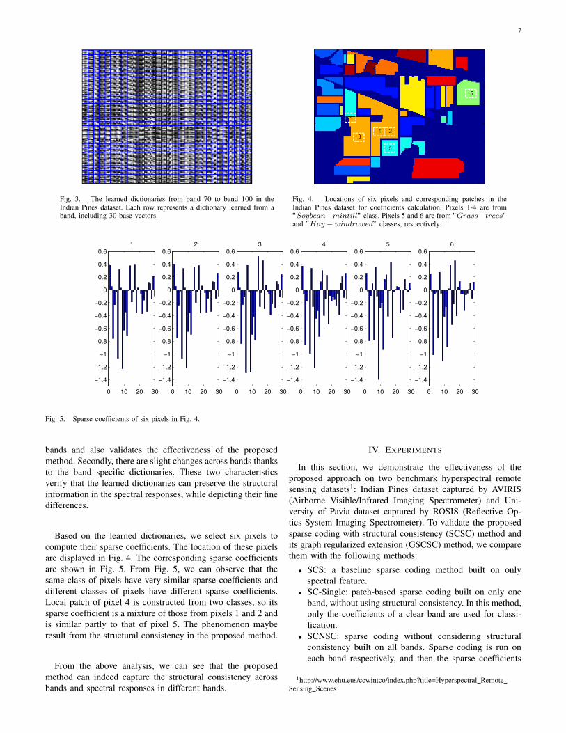
To get better understanding of the learned dictionaries andcoefficients, we analyse the outcome of the proposed methodon the Indian Pines dataset. In this experiment, the size ofdictionary is set to 30. Image patches of size 9 × 9 centeredat each pixel are used as the input. Fig. 3 shows the obtaineddictionaries from the 70th to the 100th bands, in which eachcell represents a base vector in a dictionary and each rowshows the dictionary learned from a band.

Two significant characteristics can be observed from thisfigure. Firstly, the dictionaries have great similarities acrossbands, which reflects the inherent structural consistency across

7

Fig. 3. The learned dictionaries from band 70 to band 100 in theIndian Pines dataset. Each row represents a dictionary learned from aband, including 30 base vectors.

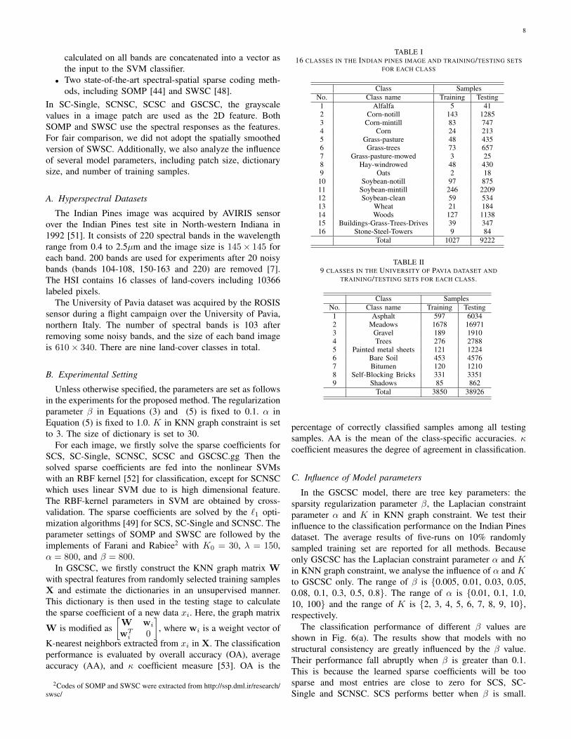
Fig. 4. Locations of six pixels and corresponding patches in theIndian Pines dataset for coefficients calculation. Pixels 1-4 are from”Soybean−mintill” class. Pixels 5 and 6 are from ”Grass−trees”and ”Hay − windrowed” classes, respectively.

0 10 20 30

−1.4

−1.2

−1

−0.8

−0.6

−0.4

−0.2

0

0.2

0.4

0.6

1

0 10 20 30

−1.4

−1.2

−1

−0.8

−0.6

−0.4

−0.2

0

0.2

0.4

0.6

2

0 10 20 30

−1.4

−1.2

−1

−0.8

−0.6

−0.4

−0.2

0

0.2

0.4

0.6

3

0 10 20 30

−1.4

−1.2

−1

−0.8

−0.6

−0.4

−0.2

0

0.2

0.4

0.6

4

0 10 20 30

−1.4

−1.2

−1

−0.8

−0.6

−0.4

−0.2

0

0.2

0.4

0.6

5

0 10 20 30

−1.4

−1.2

−1

−0.8

−0.6

−0.4

−0.2

0

0.2

0.4

0.6

6

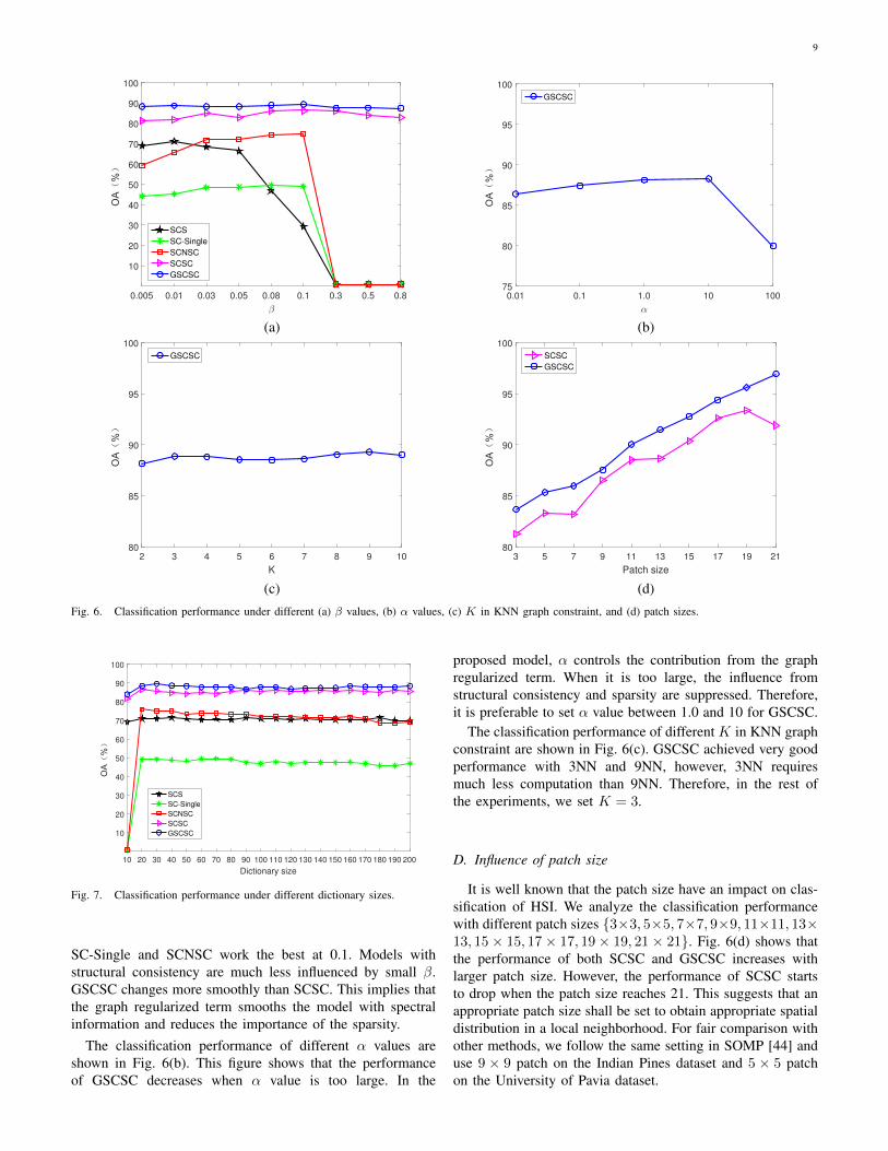
Fig. 5. Sparse coefficients of six pixels in Fig. 4.

bands and also validates the effectiveness of the proposedmethod. Secondly, there are slight changes across bands thanksto the band specific dictionaries. These two characteristicsverify that the learned dictionaries can preserve the structuralinformation in the spectral responses, while depicting their finedifferences.

Based on the learned dictionaries, we select six pixels tocompute their sparse coefficients. The location of these pixelsare displayed in Fig. 4. The corresponding sparse coefficientsare shown in Fig. 5. From Fig. 5, we can observe that thesame class of pixels have very similar sparse coefficients anddifferent classes of pixels have different sparse coefficients.Local patch of pixel 4 is constructed from two classes, so itssparse coefficient is a mixture of those from pixels 1 and 2 andis similar partly to that of pixel 5. The phenomenon mayberesult from the structural consistency in the proposed method.

From the above analysis, we can see that the proposedmethod can indeed capture the structural consistency acrossbands and spectral responses in different bands.

IV. EXPERIMENTS

In this section, we demonstrate the effectiveness of theproposed approach on two benchmark hyperspectral remotesensing datasets1: Indian Pines dataset captured by AVIRIS(Airborne Visible/Infrared Imaging Spectrometer) and Uni-versity of Pavia dataset captured by ROSIS (Reflective Op-tics System Imaging Spectrometer). To validate the proposedsparse coding with structural consistency (SCSC) method andits graph regularized extension (GSCSC) method, we comparethem with the following methods:

• SCS: a baseline sparse coding method built on onlyspectral feature.

• SC-Single: patch-based sparse coding built on only oneband, without using structural consistency. In this method,only the coefficients of a clear band are used for classi-fication.

• SCNSC: sparse coding without considering structuralconsistency built on all bands. Sparse coding is run oneach band respectively, and then the sparse coefficients

1http://www.ehu.eus/ccwintco/index.php?title=Hyperspectral RemoteSensing Scenes

8

calculated on all bands are concatenated into a vector asthe input to the SVM classifier.

• Two state-of-the-art spectral-spatial sparse coding meth-ods, including SOMP [44] and SWSC [48].

In SC-Single, SCNSC, SCSC and GSCSC, the grayscalevalues in a image patch are used as the 2D feature. BothSOMP and SWSC use the spectral responses as the features.For fair comparison, we did not adopt the spatially smoothedversion of SWSC. Additionally, we also analyze the influenceof several model parameters, including patch size, dictionarysize, and number of training samples.

A. Hyperspectral Datasets

The Indian Pines image was acquired by AVIRIS sensorover the Indian Pines test site in North-western Indiana in1992 [51]. It consists of 220 spectral bands in the wavelengthrange from 0.4 to 2.5µm and the image size is 145× 145 foreach band. 200 bands are used for experiments after 20 noisybands (bands 104-108, 150-163 and 220) are removed [7].The HSI contains 16 classes of land-covers including 10366labeled pixels.

The University of Pavia dataset was acquired by the ROSISsensor during a flight campaign over the University of Pavia,northern Italy. The number of spectral bands is 103 afterremoving some noisy bands, and the size of each band imageis 610× 340. There are nine land-cover classes in total.

B. Experimental Setting

Unless otherwise specified, the parameters are set as followsin the experiments for the proposed method. The regularizationparameter β in Equations (3) and (5) is fixed to 0.1. α inEquation (5) is fixed to 1.0. K in KNN graph constraint is setto 3. The size of dictionary is set to 30.

For each image, we firstly solve the sparse coefficients forSCS, SC-Single, SCNSC, SCSC and GSCSC.gg Then thesolved sparse coefficients are fed into the nonlinear SVMswith an RBF kernel [52] for classification, except for SCNSCwhich uses linear SVM due to is high dimensional feature.The RBF-kernel parameters in SVM are obtained by cross-validation. The sparse coefficients are solved by the `1 opti-mization algorithms [49] for SCS, SC-Single and SCNSC. Theparameter settings of SOMP and SWSC are followed by theimplements of Farani and Rabiee2 with K0 = 30, λ = 150,α = 800, and β = 800.

In GSCSC, we firstly construct the KNN graph matrix Wwith spectral features from randomly selected training samplesX and estimate the dictionaries in an unsupervised manner.This dictionary is then used in the testing stage to calculatethe sparse coefficient of a new data xi. Here, the graph matrix

W is modified as[W wi

wTi 0

], where wi is a weight vector of

K-nearest neighbors extracted from xi in X. The classificationperformance is evaluated by overall accuracy (OA), averageaccuracy (AA), and κ coefficient measure [53]. OA is the

2Codes of SOMP and SWSC were extracted from http://ssp.dml.ir/research/swsc/

TABLE I16 CLASSES IN THE INDIAN PINES IMAGE AND TRAINING/TESTING SETS

FOR EACH CLASS

Class SamplesNo. Class name Training Testing1 Alfalfa 5 412 Corn-notill 143 12853 Corn-mintill 83 7474 Corn 24 2135 Grass-pasture 48 4356 Grass-trees 73 6577 Grass-pasture-mowed 3 258 Hay-windrowed 48 4309 Oats 2 1810 Soybean-notill 97 87511 Soybean-mintill 246 220912 Soybean-clean 59 53413 Wheat 21 18414 Woods 127 113815 Buildings-Grass-Trees-Drives 39 34716 Stone-Steel-Towers 9 84

Total 1027 9222

TABLE II9 CLASSES IN THE UNIVERSITY OF PAVIA DATASET AND

TRAINING/TESTING SETS FOR EACH CLASS.

Class SamplesNo. Class name Training Testing1 Asphalt 597 60342 Meadows 1678 169713 Gravel 189 19104 Trees 276 27885 Painted metal sheets 121 12246 Bare Soil 453 45767 Bitumen 120 12108 Self-Blocking Bricks 331 33519 Shadows 85 862

Total 3850 38926

percentage of correctly classified samples among all testingsamples. AA is the mean of the class-specific accuracies. κcoefficient measures the degree of agreement in classification.

C. Influence of Model parameters

In the GSCSC model, there are tree key parameters: thesparsity regularization parameter β, the Laplacian constraintparameter α and K in KNN graph constraint. We test theirinfluence to the classification performance on the Indian Pinesdataset. The average results of five-runs on 10% randomlysampled training set are reported for all methods. Becauseonly GSCSC has the Laplacian constraint parameter α and Kin KNN graph constraint, we analyse the influence of α and Kto GSCSC only. The range of β is {0.005, 0.01, 0.03, 0.05,0.08, 0.1, 0.3, 0.5, 0.8}. The range of α is {0.01, 0.1, 1.0,10, 100} and the range of K is {2, 3, 4, 5, 6, 7, 8, 9, 10},respectively.

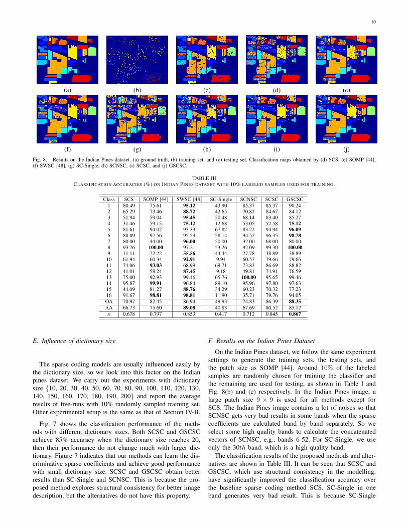
The classification performance of different β values areshown in Fig. 6(a). The results show that models with nostructural consistency are greatly influenced by the β value.Their performance fall abruptly when β is greater than 0.1.This is because the learned sparse coefficients will be toosparse and most entries are close to zero for SCS, SC-Single and SCNSC. SCS performs better when β is small.

9

0.005 0.01 0.03 0.05 0.08 0.1 0.3 0.5 0.8

β

10

20

30

40

50

60

70

80

90

100

SCS

SC-Single

SCNSC

SCSC

GSCSC

0.01 0.1 1.0 10 100

α

75

80

85

90

95

100

GSCSC

(a) (b)

2 3 4 5 6 7 8 9 10

K

80

85

90

95

100

GSCSC

3 5 7 9 11 13 15 17 19 21

Patch size

80

85

90

95

100

SCSC

GSCSC

(c) (d)

Fig. 6. Classification performance under different (a) β values, (b) α values, (c) K in KNN graph constraint, and (d) patch sizes.

10 20 30 40 50 60 70 80 90 100 110 120 130 140 150 160 170 180 190 200

Dictionary size

10

20

30

40

50

60

70

80

90

100

SCS

SC-Single

SCNSC

SCSC

GSCSC

Fig. 7. Classification performance under different dictionary sizes.

SC-Single and SCNSC work the best at 0.1. Models withstructural consistency are much less influenced by small β.GSCSC changes more smoothly than SCSC. This implies thatthe graph regularized term smooths the model with spectralinformation and reduces the importance of the sparsity.

The classification performance of different α values areshown in Fig. 6(b). This figure shows that the performanceof GSCSC decreases when α value is too large. In the

proposed model, α controls the contribution from the graphregularized term. When it is too large, the influence fromstructural consistency and sparsity are suppressed. Therefore,it is preferable to set α value between 1.0 and 10 for GSCSC.

The classification performance of different K in KNN graphconstraint are shown in Fig. 6(c). GSCSC achieved very goodperformance with 3NN and 9NN, however, 3NN requiresmuch less computation than 9NN. Therefore, in the rest ofthe experiments, we set K = 3.

D. Influence of patch size

It is well known that the patch size have an impact on clas-sification of HSI. We analyze the classification performancewith different patch sizes {3×3, 5×5, 7×7, 9×9, 11×11, 13×13, 15 × 15, 17 × 17, 19 × 19, 21 × 21}. Fig. 6(d) shows thatthe performance of both SCSC and GSCSC increases withlarger patch size. However, the performance of SCSC startsto drop when the patch size reaches 21. This suggests that anappropriate patch size shall be set to obtain appropriate spatialdistribution in a local neighborhood. For fair comparison withother methods, we follow the same setting in SOMP [44] anduse 9 × 9 patch on the Indian Pines dataset and 5 × 5 patchon the University of Pavia dataset.

10

(a) (b) (c) (d) (e)

(f) (g) (h) (i) (j)Fig. 8. Results on the Indian Pines dataset. (a) ground truth, (b) training set, and (c) testing set. Classification maps obtained by (d) SCS, (e) SOMP [44],(f) SWSC [48], (g) SC-Single, (h) SCNSC, (i) SCSC, and (j) GSCSC.

TABLE IIICLASSIFICATION ACCURACIES (%) ON INDIAN PINES DATASET WITH 10% LABELED SAMPLES USED FOR TRAINING.

Class SCS SOMP [44] SWSC [48] SC-Single SCNSC SCSC GSCSC1 80.49 75.61 95.12 43.90 85.37 85.37 90.242 65.29 73.46 88.72 42.65 70.82 84.67 84.123 51.94 59.04 95.45 20.48 68.14 83.40 85.274 31.46 59.15 75.12 12.68 53.05 52.58 75.125 81.61 94.02 93.33 67.82 83.22 94.94 96.096 88.89 97.56 95.59 58.14 94.52 96.35 98.787 80.00 44.00 96.00 20.00 32.00 68.00 80.008 93.26 100.00 97.21 53.26 92.09 99.30 100.009 11.11 22.22 55.56 44.44 27.78 38.89 38.8910 61.94 60.34 92.91 9.94 60.57 79.66 79.6611 74.06 93.03 68.99 69.71 73.83 86.69 88.8212 41.01 58.24 87.45 9.18 49.81 74.91 76.5913 75.00 92.93 99.46 65.76 100.00 95.65 99.4614 95.87 99.91 96.84 89.10 95.96 97.80 97.6315 44.09 81.27 88.76 34.29 60.23 70.32 77.2316 91.67 98.81 98.81 11.90 35.71 79.76 94.05OA 70.97 82.45 86.94 49.93 74.83 86.39 88.35AA 66.73 75.60 89.08 40.83 67.69 80.52 85.12κ 0.678 0.797 0.853 0.417 0.712 0.845 0.867

E. Influence of dictionary size

The sparse coding models are usually influenced easily bythe dictionary size, so we look into this factor on the Indianpines dataset. We carry out the experiments with dictionarysize {10, 20, 30, 40, 50, 60, 70, 80, 90, 100, 110, 120, 130,140, 150, 160, 170, 180, 190, 200} and report the averageresults of five-runs with 10% randomly sampled training set.Other experimental setup is the same as that of Section IV-B.

Fig. 7 shows the classification performance of the meth-ods with different dictionary sizes. Both SCSC and GSCSCachieve 85% accuracy when the dictionary size reaches 20,then their performance do not change much with larger dic-tionary. Figure 7 indicates that our methods can learn the dis-criminative sparse coefficients and achieve good performancewith small dictionary size. SCSC and GSCSC obtain betterresults than SC-Single and SCNSC. This is because the pro-posed method explores structural consistency for better imagedescription, but the alternatives do not have this property.

F. Results on the Indian Pines Dataset

On the Indian Pines dataset, we follow the same experimentsettings to generate the training sets, the testing sets, andthe patch size as SOMP [44]. Around 10% of the labeledsamples are randomly chosen for training the classifier andthe remaining are used for testing, as shown in Table I andFig. 8(b) and (c) respectively. In the Indian Pines image, alarge patch size 9 × 9 is used for all methods except forSCS. The Indian Pines image contains a lot of noises so thatSCNSC gets very bad results in some bands when the sparsecoefficients are calculated band by band separately. So weselect some high quality bands to calculate the concatenatedvectors of SCNSC, e.g., bands 6-52. For SC-Single, we useonly the 30th band, which is a high quality band.

The classification results of the proposed methods and alter-natives are shown in Table III. It can be seen that SCSC andGSCSC, which use structural consistency in the modelling,have significantly improved the classification accuracy overthe baseline sparse coding method SCS. SC-Single in oneband generates very bad result. This is because SC-Single

11

(a) (b) (c) (d) (e)

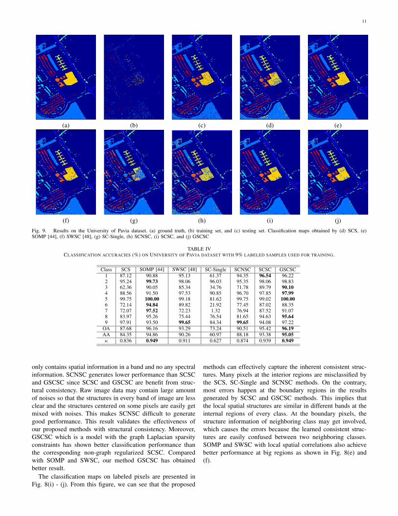
(f) (g) (h) (i) (j)Fig. 9. Results on the University of Pavia dataset. (a) ground truth, (b) training set, and (c) testing set. Classification maps obtained by (d) SCS, (e)SOMP [44], (f) SWSC [48], (g) SC-Single, (h) SCNSC, (i) SCSC, and (j) GSCSC

TABLE IVCLASSIFICATION ACCURACIES (%) ON UNIVERSITY OF PAVIA DATASET WITH 9% LABELED SAMPLES USED FOR TRAINING.

Class SCS SOMP [44] SWSC [48] SC-Single SCNSC SCSC GSCSC1 87.12 90.88 95.13 61.37 94.35 96.54 96.222 95.24 99.73 98.06 96.03 95.35 98.06 98.833 62.36 90.05 85.34 34.76 71.78 89.79 90.104 88.56 91.50 97.53 90.85 96.70 97.85 97.995 99.75 100.00 99.18 81.62 99.75 99.02 100.006 72.14 94.84 89.82 21.92 77.45 87.02 88.357 72.07 97.52 72.23 1.32 76.94 87.52 91.078 83.97 95.26 75.44 76.54 81.65 94.63 95.649 97.91 93.50 99.65 84.34 99.65 94.08 97.22

OA 87.68 96.16 93.29 73.24 90.51 95.42 96.19AA 84.35 94.86 90.26 60.97 88.18 93.38 95.05κ 0.836 0.949 0.911 0.627 0.874 0.939 0.949

only contains spatial information in a band and no any spectralinformation. SCNSC generates lower performance than SCSCand GSCSC since SCSC and GSCSC are benefit from struc-tural consistency. Raw image data may contain large amountof noises so that the structures in every band of image are lessclear and the structures centered on some pixels are easily getmixed with noises. This makes SCNSC difficult to generategood performance. This result validates the effectiveness ofour proposed methods with structural consistency. Moreover,GSCSC which is a model with the graph Laplacian sparsityconstraints has shown better classification performance thanthe corresponding non-graph regularized SCSC. Comparedwith SOMP and SWSC, our method GSCSC has obtainedbetter result.

The classification maps on labeled pixels are presented inFig. 8(i) - (j). From this figure, we can see that the proposed

methods can effectively capture the inherent consistent struc-tures. Many pixels at the interior regions are misclassified bythe SCS, SC-Single and SCNSC methods. On the contrary,most errors happen at the boundary regions in the resultsgenerated by SCSC and GSCSC methods. This implies thatthe local spatial structures are similar in different bands at theinternal regions of every class. At the boundary pixels, thestructure information of neighboring class may get involved,which causes the errors because the learned consistent struc-tures are easily confused between two neighboring classes.SOMP and SWSC with local spatial correlations also achievebetter performance at big regions as shown in Fig. 8(e) and(f).

12

G. Results on the University of Pavia Dataset

We use the same experimental settings as in [44] to generatethe training set, the testing set and the patch size on theUniversity of Pavia dataset. Around 9% of the labeled samplesare randomly chosen for training and the remaining are usedfor testing. More detailed information on the training andtesting sets are shown in Table II and Fig. 9(b) and (c).Considering the small spatial homogeneity in the Universityof Pavia image, a small patch size of 5×5 is used all methodsexcept SCS. SCNSC uses all bands of sparse coefficients andconcatenates them into a vector.

The classification results of various methods are presented inTable IV. Fig. 9(d) - (j) gives the classification maps on labeledpixels. The proposed methods achieve great improvement overthe baseline SCS and are better than SC-Single and SCNSCwith no structural consistency. They also generate slightlyhigher performance than SOMP and SWSC which are basedon spatial correlations. From Fig. 9, we can see that the“Meadows” class at the bottom of the HSI is a large regionand its internal pixels should have similar spatial structureand spectral information. Therefore, most pixels in this classare classified correctly by our methods. Because SCS capturesonly spectral information and SCNSC uses only spatial infor-mation, they are strongly influenced by the noises in differentbands. The proposed methods explore spatial consistency andenforce the spatial structures along the spectral dimension, andthus show many advantages in the classification.

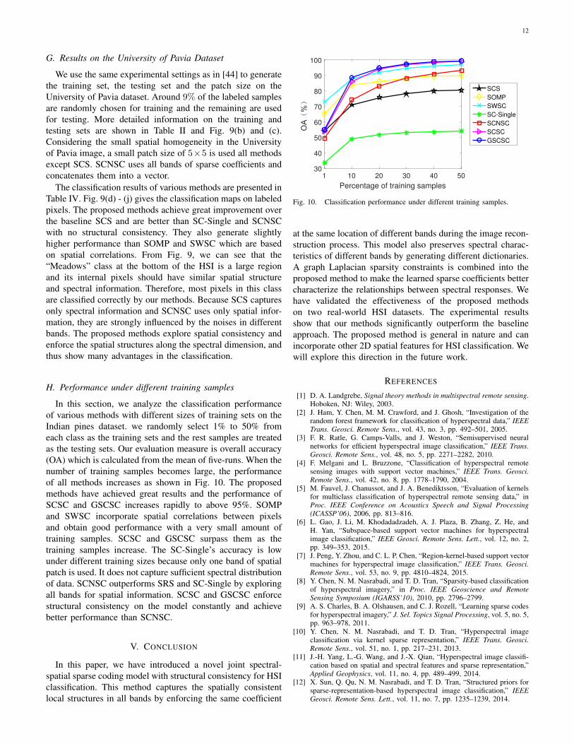
H. Performance under different training samples

In this section, we analyze the classification performanceof various methods with different sizes of training sets on theIndian pines dataset. we randomly select 1% to 50% fromeach class as the training sets and the rest samples are treatedas the testing sets. Our evaluation measure is overall accuracy(OA) which is calculated from the mean of five-runs. When thenumber of training samples becomes large, the performanceof all methods increases as shown in Fig. 10. The proposedmethods have achieved great results and the performance ofSCSC and GSCSC increases rapidly to above 95%. SOMPand SWSC incorporate spatial correlations between pixelsand obtain good performance with a very small amount oftraining samples. SCSC and GSCSC surpass them as thetraining samples increase. The SC-Single’s accuracy is lowunder different training sizes because only one band of spatialpatch is used. It does not capture sufficient spectral distributionof data. SCNSC outperforms SRS and SC-Single by exploringall bands for spatial information. SCSC and GSCSC enforcestructural consistency on the model constantly and achievebetter performance than SCNSC.

V. CONCLUSION

In this paper, we have introduced a novel joint spectral-spatial sparse coding model with structural consistency for HSIclassification. This method captures the spatially consistentlocal structures in all bands by enforcing the same coefficient

1 10 20 30 40 50

Percentage of training samples

30

40

50

60

70

80

90

100

SCS

SOMP

SWSC

SC-Single

SCNSC

SCSC

GSCSC

Fig. 10. Classification performance under different training samples.

at the same location of different bands during the image recon-struction process. This model also preserves spectral charac-teristics of different bands by generating different dictionaries.A graph Laplacian sparsity constraints is combined into theproposed method to make the learned sparse coefficients bettercharacterize the relationships between spectral responses. Wehave validated the effectiveness of the proposed methodson two real-world HSI datasets. The experimental resultsshow that our methods significantly outperform the baselineapproach. The proposed method is general in nature and canincorporate other 2D spatial features for HSI classification. Wewill explore this direction in the future work.

REFERENCES

[1] D. A. Landgrebe, Signal theory methods in multispectral remote sensing.Hoboken, NJ: Wiley, 2003.

[2] J. Ham, Y. Chen, M. M. Crawford, and J. Ghosh, “Investigation of therandom forest framework for classification of hyperspectral data,” IEEETrans. Geosci. Remote Sens., vol. 43, no. 3, pp. 492–501, 2005.

[3] F. R. Ratle, G. Camps-Valls, and J. Weston, “Semisupervised neuralnetworks for efficient hyperspectral image classification,” IEEE Trans.Geosci. Remote Sens., vol. 48, no. 5, pp. 2271–2282, 2010.

[4] F. Melgani and L. Bruzzone, “Classification of hyperspectral remotesensing images with support vector machines,” IEEE Trans. Geosci.Remote Sens., vol. 42, no. 8, pp. 1778–1790, 2004.

[5] M. Fauvel, J. Chanussot, and J. A. Benediktsson, “Evaluation of kernelsfor multiclass classification of hyperspectral remote sensing data,” inProc. IEEE Conference on Acoustics Speech and Signal Processing(ICASSP’06), 2006, pp. 813–816.

[6] L. Gao, J. Li, M. Khodadadzadeh, A. J. Plaza, B. Zhang, Z. He, andH. Yan, “Subspace-based support vector machines for hyperspectralimage classification,” IEEE Geosci. Remote Sens. Lett., vol. 12, no. 2,pp. 349–353, 2015.

[7] J. Peng, Y. Zhou, and C. L. P. Chen, “Region-kernel-based support vectormachines for hyperspectral image classification,” IEEE Trans. Geosci.Remote Sens., vol. 53, no. 9, pp. 4810–4824, 2015.

[8] Y. Chen, N. M. Nasrabadi, and T. D. Tran, “Sparsity-based classificationof hyperspectral imagery,” in Proc. IEEE Geoscience and RemoteSensing Symposium (IGARSS’10), 2010, pp. 2796–2799.

[9] A. S. Charles, B. A. Olshausen, and C. J. Rozell, “Learning sparse codesfor hyperspectral imagery,” J. Sel. Topics Signal Processing, vol. 5, no. 5,pp. 963–978, 2011.

[10] Y. Chen, N. M. Nasrabadi, and T. D. Tran, “Hyperspectral imageclassification via kernel sparse representation,” IEEE Trans. Geosci.Remote Sens., vol. 51, no. 1, pp. 217–231, 2013.

[11] J.-H. Yang, L.-G. Wang, and J.-X. Qian, “Hyperspectral image classifi-cation based on spatial and spectral features and sparse representation,”Applied Geophysics, vol. 11, no. 4, pp. 489–499, 2014.

[12] X. Sun, Q. Qu, N. M. Nasrabadi, and T. D. Tran, “Structured priors forsparse-representation-based hyperspectral image classification,” IEEEGeosci. Remote Sens. Lett., vol. 11, no. 7, pp. 1235–1239, 2014.

13

[13] L. He, Y. Li, X. Li, and W. Wu, “Spectral-spatial classification of hy-perspectral images via spatial translation-invariant wavelet-based sparserepresentation,” IEEE Trans. Geosci. Remote Sens., vol. 53, no. 5, pp.2696–2712, 2015.

[14] M. E. Midhun, S. R. Nair, V. T. N. Prabhakar, and S. S. Kumar, “Deepmodel for classification of hyperspectral image using restricted Boltz-mann machine,” in Proc. International Conference on InterdisciplinaryAdvances in Applied Computing, 2014, pp. 1–7.

[15] Y. Chen, X. Zhao, and X. Jia, “Spectralcspatial classification of hyper-spectral data based on deep belief network,” IEEE J. Sel. Topics Appl.Earth Observ. Remote Sens., vol. 8, no. 6, pp. 2381–2392, 2015.

[16] A. Plaza, J. A. Benediktsson, J. W. Boardman, J. Brazile, L. Bruzzone,G. Camps-Valls, J. Chanussot, M. Fauvel, P. Gamba, A. Gualtieri,M. Marconcini, J. C. Tilton, and G. Trianni, “Recent advances intechniques for hyperspectral image processing,” Remote Sensing ofEnvironment, vol. 113, no. 9, pp. S110–S122, 2009.

[17] U. Srinivas, Y. Chen, V. Monga, N. M. Nasrabadi, and T. D. Tran,“Exploiting sparsity in hyperspectral image classification via graphicalmodels,” IEEE Geosci. Remote Sensing Lett., vol. 10, no. 3, pp. 505–509, 2013.

[18] Z. tao Qin, W. nian Yang, R. Yang, X. yu Zhao, and T. jiao Yang,“Dictionary-based, clustered sparse representation for hyperspectral im-age classification,” Journal of Spectroscopy, 2015.

[19] W. Li, Q. Du, F. Zhang, and W. Hu, “Hyperspectral image classificationby fusing collaborative and sparse representations,” IEEE J. Sel. TopicsAppl. Earth Observ. Remote Sens., vol. PP, no. 99, pp. 1–20, 2016.

[20] M. Fauvel, Y. Tarabalka, J. A. Benediktsson, J. Chanussot, and J. C.Tilton, “Advances in spectral-spatial classification of hyperspectral im-ages,” Proceedings of the IEEE, vol. 101, no. 3, pp. 652–675, 2013.

[21] Z. H. Nezhad, A. Karami, R. Heylen, and P. Scheunders, “Fusion ofhyperspectral and multispectral images using spectral unmixing andsparse coding,” IEEE J. Sel. Topics Appl. Earth Observ. Remote Sens.,vol. 9, no. 6, pp. 2377–2389, 2016.

[22] M. D. Mura, A. Villa, J. A. Benediktsson, J. Chanussot, and L. Bruzzone,“Classification of hyperspectral images by using extended morphologicalattribute profiles and independent component analysis,” IEEE Geosci.Remote Sens. Lett., vol. 8, no. 3, pp. 542–546, 2011.

[23] P. Ghamisi, M. D. Mura, and J. A. Benediktsson, “A survey on spectral-spatial classification techniques based on attribute profiles,” IEEE Trans.Geosci. Remote Sens., vol. 53, no. 5, pp. 2335–2353, 2015.

[24] X. Jia and J. Richards, “Managing the spectral-spatial mix in contextclassification using Markov random fields,” IEEE Geosci. Remote Sens.Lett., vol. 5, pp. 311–314, 2008.

[25] J. Xia, J. Chanussot, P. Du, and X. He, “Spectral-spatial classificationfor hyperspectral data using rotation forests with local feature extractionand Markov random fields,” IEEE Trans. Geosci. Remote Sens., vol. 53,no. 5, pp. 2532–2546, 2015.

[26] Y. Qian, M. Ye, and J. Zhou, “Hyperspectral image classification basedon structured sparse logistic regression and three-dimensional wavelettexture features,” IEEE Trans. Geosci. Remote Sens., vol. 51, no. 4-2,pp. 2276–2291, 2013.

[27] J. Liu, Z. Wu, Z. Wei, L. Xiao, and L. Sun, “Spatial-spectral kernelsparse representation for hyperspectral image classification,” IEEE J.Sel. Topics Appl. Earth Observ. Remote Sens., vol. 6, no. 6, pp. 2462–2471, Dec 2013.

[28] Z. He, Q. Wang, Y. Shen, and M. Sun, “Kernel sparse multitasklearning for hyperspectral image classification with empirical modedecomposition and morphological wavelet-based features,” IEEE Trans.Geosci. Remote Sens., vol. 52, no. 8, pp. 5150–5163, 2014.

[29] H. Zhang, J. Li, Y. Huang, and L. Zhang, “A nonlocal weighted jointsparse representation classification method for hyperspectral imagery,”IEEE J. Sel. Topics Appl. Earth Observ. Remote Sens., vol. 7, no. 6, pp.2056–2065, 2014.

[30] J. Wang, L. Jiao, H. Liu, S. Yang, and F. Liu, “Hyperspectral imageclassification by spatialcspectral derivative-aided kernel joint sparserepresentation,” IEEE J. Sel. Topics Appl. Earth Observ. Remote Sens.,vol. 8, no. 6, pp. 2485–2500, June 2015.

[31] S. Jia, J. Hu, Y. Xie, L. Shen, X. Jia, and Q. Li, “Gabor cube selectionbased multitask joint sparse representation for hyperspectral imageclassification,” IEEE Trans. Geosci. Remote Sens., vol. 54, no. 6, pp.3174–3187, 2016.

[32] Z. Xue, P. Du, J. Li, and H. Su, “Simultaneous sparse graph embeddingfor hyperspectral image classification,” IEEE Trans. Geosci. RemoteSens., vol. 53, no. 11, pp. 6114–6133, 2015.

[33] J. Wright, A. Y. Yang, A. Ganesh, S. S. Sastry, and Y. Ma, “Robust facerecognition via sparse representation,” IEEE Trans. Pattern Anal. Mach.Intell., vol. 31, no. 2, pp. 210–227, 2009.

[34] J. Wright, Y. Ma, J. Mairal, G. Sapiro, T. S. Huang, and S. Yan, “Sparserepresentation for computer vision and pattern recognition,” Proceedingsof the IEEE, vol. 98, no. 6, pp. 1031–1044, 2010.

[35] Z. Shu, J. Zhou, P. Huang, X. Yu, Z. Yang, and C. Zhao, “Local andglobal regularized sparse coding for data representation,” Neurocomput-ing, vol. 175, pp. 188–197, 2016.

[36] M. Zheng, J. Bu, C. Chen, C. Wang, L. Zhang, G. Qiu, and D. Cai,“Graph regularized sparse coding for image representation,” IEEE Trans.Image Process., vol. 20, no. 5, pp. 1327–1336, 2011.

[37] S. Gao, I. W.-H. Tsang, and L.-T. Chia, “Laplacian sparse coding,hypergraph laplacian sparse coding, and applications,” IEEE Trans.Pattern Anal. Mach. Intell., vol. 35, no. 1, pp. 92–104, 2013.

[38] L. Tong, J. Zhou, X. Bai, and Y. Gao, “Dual graph regularized NMF forhyperspectral unmixing,” in Proc. International Conference on DigitalImage Computing: Techniques and Applications, 2014, pp. 1–8.

[39] Z. Shu, J. Zhou, L. Tong, X. Bai, and C. Zhao, “Multilayer manifold andsparsity constrainted nonnegative matrix factorization for hyperspectralunmixing,” in Proc. IEEE Conference on Image Processing (ICIP’15),2015, pp. 2174–2178.

[40] E. Berg and M. P. Friedlander, “Joint-sparse recovery from multiplemeasurements,” IEEE Trans. Inf. Theory, vol. 56, no. 5, pp. 2516–2527,2010.

[41] A. Rakotomamonjy, “Surveying and comparing simultaneous sparseapproximation (or group-lasso) algorithms,” Signal Processing, vol. 91,no. 7, pp. 1505–1526, 2011.

[42] G. Liu, Z. Lin, S. Yan, J. Sun, Y. Yu, and Y. Ma, “Robust recoveryof subspace structures by low-rank representation,” IEEE Trans. PatternAnal. Mach. Intell., vol. 35, no. 1, pp. 171–184, 2013.

[43] M. Ye, Y. Qian, and J. Zhou, “Multitask sparse nonnegative matrixfactorization for joint spectral-spatial hyperspectral imagery denoising,”IEEE Trans. Geosci. Remote Sens., vol. 53, no. 5, pp. 2621–2639, 2015.

[44] Y. Chen, N. M. Nasrabadi, and T. D. Tran, “Hyperspectral imageclassification using dictionary-based sparse representation,” IEEE Trans.Geosci. Remote Sens., vol. 49, no. 10, pp. 3973–3985, 2011.

[45] S. Jia, X. Zhang, and Q. Li, “Spectralspatial hyperspectral imageclassification using `1/2 regularized low-rank representation and sparserepresentation-based graph cuts,” IEEE J. Sel. Topics Appl. EarthObserv. Remote Sens., vol. 8, no. 6, pp. 2473–2484, 2015.

[46] H. Yuan and Y. Y. Tang, “Sparse representation based on set-to-setdistance for hyperspectral image classification,” IEEE J. Sel. Topics Appl.Earth Observ. Remote Sens., vol. 8, no. 6, pp. 2464–2472, 2015.

[47] E. Zhang, L. Jiao, X. Zhang, H. Liu, and S. Wang, “Class-leveljoint sparse representation for multifeature-based hyperspectral imageclassification,” IEEE J. Sel. Topics Appl. Earth Observ. Remote Sens.,vol. PP, no. 99, pp. 1–18, 2016.

[48] A. S. Farani and H. R. Rabiee, “When pixels team up: Spatially weightedsparse coding for hyperspectral image classification,” IEEE Geosci.Remote Sens. Lett., vol. 12, no. 1, pp. 107–111, 2015.

[49] H. Lee, A. Battle, R. Raina, and A. Y. Ng, “Efficient sparse coding al-gorithms,” in Proc. Advances in Neural Information Processing Systems(NIPS’06), 2006, pp. 801–808.

[50] R. Fletcher, Practical methods of optimization. Hoboken, NJ: Wiley,1987.

[51] VIRIS NW Indianas Indian Pines 1992 data set. [Online]. Available:http://cobweb.ecn.purdue.edu/biehl/MultiSpec/documentation.html

[52] C.-C. Chang and C.-J. Lin, “LIBSVM: A library for support vectormachines,” ACM Transactions on Intelligent Systems and Technology,vol. 2, no. 3, pp. 389–396, 2011.

[53] J. A. Richards, Remote Sensing Digital Image Analysis: An Introduction,5th ed. New York, NY, USA: Springer Berlin Heidelberg, 2013.

14

Changhong Liu received the B.S. and M.S. degreesin computer science from Jiangxi Normal University,Nanchang, China, in 2000 and 2004, respectively,and the Ph.D. degree in computer application tech-nology from University of Science & TechnologyBeijing, Beijing, China, in 2011.

She is currently a lecturer in the School of Com-puter and Information Engineering, Jiangxi NormalUniversity, China. During 2015, she was a VisitingFellow in the School of Information and Commu-nication Technology at Griffith University, Nathan,

Australia. Her research interests include pattern recognition, hyperspectralimaging, computer vision, and machine learning.

Jun Zhou received the B.S. degree in computerscience and the B.E. degree in international businessfrom Nanjing University of Science and Technology,Nanjing, China, in 1996 and 1998, respectively. Hereceived the M.S. degree in computer science fromConcordia University, Montreal, Canada, in 2002,and the Ph.D. degree from the University of Alberta,Edmonton, Canada, in 2006.

He is a senior lecturer in the School of Infor-mation and Communication Technology at GriffithUniversity, Nathan, Australia. Previously, he had

been a research fellow in the Research School of Computer Science atthe Australian National University, Canberra, Australia, and a researcher inthe Canberra Research Laboratory, NICTA, Australia. His research interestsinclude pattern recognition, computer vision and spectral imaging with theirapplications to remote sensing and environmental informatics.

Jie Liang Jie Liang received the B.E. degree inautomatic control from National University of De-fense Technology, Changsha, China, in 2011. He iscurrently working toward the Ph.D. degree in theResearch School of Engineering, Australian NationalUniversity, Canberra, Australia. He is also a visitingscholar in the School of Information of Commu-nication Technology at Griffith University, Nathan,Australia.

His research topic is spectral-spatial feature ex-traction for hyperspectral image classification.

Yuntao Qian (M’04) received the B.E. and M.E.degrees in automatic control from Xi’an JiaotongUniversity, Xi’an, China, in 1989 and 1992, respec-tively, and the Ph.D. degree in signal processingfrom Xidian University, Xi’an, China, in 1996.

During 1996–1998, he was a Postdoctoral Fel-low with the Northwestern Polytechnical University,Xi’an, China. Since 1998, he has been with theCollege of Computer Science, Zhejiang University,Hangzhou, China, where he is currently a Profes-sor in computer science. During 1999–2001, 2006,

2010, and 2013, he was a Visiting Professor at Concordia University, HongKong Baptist University, Carnegie Mellon University, the Canberra ResearchLaboratory of NICTA, and Griffith University. His current research interestsinclude machine learning, signal and image processing, pattern recognition,and hyperspectral imaging.

Prof. Qian is an Associate Editor of the IEEE JOURNAL OF SELECTEDTOPICS IN APPLIED EARTH OBSERVATIONS AND REMOTE SENSING

Hanxi Li received the B.Sc. and M.Sc. degrees fromthe School of Automation Science and ElectricalEngineering, Beihang University, Beijing, China, in2004 and 2007 respectively, and the Ph.D. degreefrom the Research School of Information Scienceand Engineering at the Australian National Univer-sity, Canberra, Australia, in 2011.

He was a Researcher at NICTA (Australia) from2011-2015. He is currently a Special Term Pro-fessor in the School of Computer and InformationEngineering, Jiangxi Normal University, China. His

recent areas of interest include visual tracking, face recognition, and deeplearning.

Yongsheng Gao received the B.Sc. and M.Sc. de-grees in electronic engineering from Zhejiang Uni-versity, Hangzhou, China, in 1985 and 1988, respec-tively, and the Ph.D. degree in computer engineeringfrom Nanyang Technological University, Singapore.He is currently a Professor with the School of En-gineering, Griffith University, Brisbane, QLD, Aus-tralia. He had been the Leader of Biosecurity Group,Queensland Research Laboratory, National ICT Aus-tralia (ARC Centre of Excellence), a consultant ofPanasonic Singapore Laboratories, and an Assistant

Professor in the School of Computer Engineering, Nanyang TechnologicalUniversity, Singapore.

His research interests include face recognition, biometrics, biosecurity, im-age retrieval, computer vision, pattern recognition, environmental informatics,and medical imaging.