Embed Size (px)
Citation preview

University of Southern Queensland
School of Civil Engineering and Surveying
Exploring the Application of
Closed Form Solutions in
Geotechnical Problems
A dissertation submitted by
Timothy Eaton
in fulfilment of
ENG4112 Research Project
towards the degree of
Bachelor of Civil Engineering
Submitted: 17th October, 2013
Supervisor: Kazem Ghabraie
Abstract
This project explores the uses, values and limitations of closed form solutions in
specific areas of geotechnical engineering. Three closed form (analytical) solutions,
Kelvin’s, Boussinesq’s and Mindlin’s solutions have been chosen and researched to
determine their applications in geotechnical engineering. These applications have
been examined with the aim to modify, further define and/or extend upon them
so that they may be applicable to new problems.
A review of research on Kelvin’s, Mindlin’s and Boussinesq’s solutions gave an
indication of the ways each of the solutions could be applied to solve for certain
problems. After noting the likeness of the solutions and the accomplishments that
had been achieved with the relatively popular Boussinesq’s soultion, the aim was
to subject the lesser known and utilised Mindlin’s solution to similar concepts.
The integration of Mindlin’s solution for a sub-surface circular loading was per-
formed and is shown here in full, something which does not appear to have been
published. From this Newmark inspired Mindlin based influence charts were gener-
ated which were found to be of little practical use. Following this the relationship
between both Boussinesq’s and Mindlin’s solutions was investigated and analysed
resulting in the production of a design chart that may be applicable to a bi-loaded
anchor system.
On a whole the work undertaken in this dissertation showed the main values of the
closed form solution in the area of stresses in soil masses were that of insight and
flexibility, and their main limitation was that of the simplifying assumptions that
were required to be made.

University of Southern Queensland
Faculty of Health, Engineering and Sciences
ENG4111/2 Research Project
Limitations of Use
The Council of the University of Southern Queensland, its Faculty of Health, En-
gineering Sciences, and the staff of the University of Southern Queensland, do
not accept any responsibility for the truth, accuracy or completeness of material
contained within or associated with this dissertation.
Persons using all or any part of this material do so at their own risk, and not at the
risk of the Council of the University of Southern Queensland, its Faculty of Health,
Engineering Sciences or the staff of the University of Southern Queensland.
This dissertation reports an educational exercise and has no purpose or validity be-
yond this exercise. The sole purpose of the course pair entitled ”Research Project”
is to contribute to the overall education within the student’s chosen degree pro-
gram. This document, the associated hardware, software, drawings, and other
material set out in the associated appendices should not be used for any other
purpose: if they are so used, it is entirely at the risk of the user.
Dean
Faculty of Health, Engineering Sciences
2

Certification of Dissertation
I certify that the ideas, designs and experimental work, results, analyses and conclu-
sions set out in this dissertation are entirely my own effort, except where otherwise
indicated and acknowledged.
I further certify that the work is original and has not been previously submitted
for assessment in any other course or institution, except where specifically stated.
Student Name: Timothy Eaton
Student Number: 0061004795
Signature: ______________________________
Date: ______________________________
3

Acknowledgements
A pass of sincere thanks is due to my supervisor, Dr. Kazem Ghabraie. For it
was his direction, ideas and willingness to help at all times that gave this thesis its
proper flow and structure. I would also like to thank him for providing me with a
topic of which I found very interesting, and one that introduced me to the academic
process in an exciting manner. Additionally a devout thanks for his assistance in
MATLAB and LaTeX coding, two things of which I did not have a high degree of
competency with by any means.
Acknowledgement also goes out to my girlfriend, Kirsty, for her support and en-
couragement. Additional thanks goes out to my family and friends for injecting
positivity during the time spent working on this dissertation.
4

Contents
1 Introduction 11
1.1 Types of Solutions . . . . . . . . . . . . . . . . . . . . . . . . . . . 11
1.2 Benefits and Limitations of the Closed Form Solution . . . . . . . . 12
2 Introduction to 2D Models 14
2.1 Plane Strain . . . . . . . . . . . . . . . . . . . . . . . . . . . . . . . 15
2.2 Plane Stress . . . . . . . . . . . . . . . . . . . . . . . . . . . . . . . 17
2.3 Axisymmetric Models . . . . . . . . . . . . . . . . . . . . . . . . . . 18
3 Solutions for Stress in Soil Masses and their Applications 20
3.1 Introduction . . . . . . . . . . . . . . . . . . . . . . . . . . . . . . . 20
3.2 Kelvin’s Solution . . . . . . . . . . . . . . . . . . . . . . . . . . . . 21
3.3 Boussinesq’s Solution . . . . . . . . . . . . . . . . . . . . . . . . . . 23
3.4 Mindlin’s Solution . . . . . . . . . . . . . . . . . . . . . . . . . . . 24
5

3.5 Applications in Geotechnical Problems . . . . . . . . . . . . . . . . 27
3.5.1 Applications in Piling . . . . . . . . . . . . . . . . . . . . . . 28
3.5.2 Applications in Anchoring . . . . . . . . . . . . . . . . . . . 29
3.5.3 Applications in Tunnelling . . . . . . . . . . . . . . . . . . . 31
3.5.4 Applications in Contact Mechanics . . . . . . . . . . . . . . 33
3.5.5 General Research and Applications . . . . . . . . . . . . . . 33
3.5.6 Summary of Applications . . . . . . . . . . . . . . . . . . . 35
4 Circular Sub-Surface Loading 36
4.1 Introduction . . . . . . . . . . . . . . . . . . . . . . . . . . . . . . . 36
4.2 Integration of Mindlin’s Solution . . . . . . . . . . . . . . . . . . . 36
4.2.1 Comparing Integrated Mindlin’s and Boussinesq’s Solutions 42
5 Exploring the Applications of the Integrated Mindlin’s Solution 44
5.1 Mindlin Based Influence Chart . . . . . . . . . . . . . . . . . . . . . 44
5.1.1 Limitations . . . . . . . . . . . . . . . . . . . . . . . . . . . 48
5.2 Stress Estimation In Bi-Loaded Anchors . . . . . . . . . . . . . . . 48
5.2.1 Example . . . . . . . . . . . . . . . . . . . . . . . . . . . . . 51
5.2.2 Graphical Approach . . . . . . . . . . . . . . . . . . . . . . 52
6

5.2.3 Cancelling All Tensile Stresses . . . . . . . . . . . . . . . . . 57
5.2.4 Forming a Single Design Chart . . . . . . . . . . . . . . . . 63
5.2.5 Conclusion and Limitations . . . . . . . . . . . . . . . . . . 66
6 Conclusions and Further Work 68
6.1 Conclusions . . . . . . . . . . . . . . . . . . . . . . . . . . . . . . . 68
6.2 Further Work . . . . . . . . . . . . . . . . . . . . . . . . . . . . . . 69
A Project Specification 74
B General 76
C MATLAB Code 79
7

List of Figures
2.1 Plane Strain (Source: http://academic.uprm.edu/pcaceres/Courses/
MechMet/MET-2B.pdf . . . . . . . . . . . . . . . . . . . . . . . . . 16
2.2 Plane Stress (Source: http://academic.uprm.edu/pcaceres/Courses/
MechMet/MET-2B.pdf) . . . . . . . . . . . . . . . . . . . . . . . . 17
2.3 Stress strain axisymmetry of a pile (Powrie 2004, pp.71). . . . . . . 18
3.1 Kelvin’s Solution for a point load P in an infinite elastic space (Pou-
los & Davis 1974, pp.16). . . . . . . . . . . . . . . . . . . . . . . . . 21
3.2 Boussinesq’s solution for a point load P acting at the surface of a
semi-infinite elastic space (Perloff & Baron 1976, pp.179). . . . . . . 23
3.3 Mindlin’s solution for a force normal to the boundary in the interior
of a semi-infinite mass (Mindlin 1936). . . . . . . . . . . . . . . . . 25
3.4 Selvadurai’s anchored rigid circular plate (Selvadurai 1979). . . . . 30
3.5 Tunnel problem (Chow 1994, pp.16). . . . . . . . . . . . . . . . . . 32
8

3.6 Dominguez (1966) detailed how the stress due to a uniform dis-
tributed load over the area of the shaded section above could be
found through integration. . . . . . . . . . . . . . . . . . . . . . . 34
4.1 A uniformly distributed vertical circular loading beneath the surface
(x-y plane). . . . . . . . . . . . . . . . . . . . . . . . . . . . . . . . 37
5.1 Table of values for creation of Newmark style Mindlin based influ-
ence chart. c/z = 0.3 and ν=0.3. . . . . . . . . . . . . . . . . . . . 45
5.2 The developed Mindlin based influence chart for c/z = 0.3 and
ν = 0.3. . . . . . . . . . . . . . . . . . . . . . . . . . . . . . . . . . 46
5.3 An isometric representation of a bi-loaded anchor system with a
Boussinesq load acting on the surface plane and a Mindlin load
acting on a parallel sub-surface plane a distance of c below. . . . . 50
5.4 Influence factor curves for eq. 4.12 . . . . . . . . . . . . . . . . . . 54
5.5 Behaviour of influence factor curves for eq. 4.12 . . . . . . . . . . . 55
5.6 Behaviour of a combined Mindlin - Boussinesq influence factor curve
against increasing depth z. c = 4m. . . . . . . . . . . . . . . . . . 56
5.7 Ratio of loads required to nullify tensile stresses at depth z. c = 4m,
R = 4m. . . . . . . . . . . . . . . . . . . . . . . . . . . . . . . . . 59
5.8 Modified to include qB/qM ratio from Figure 5.7, the combined
Mindlin - Boussinesq influence factor curve against increasing depth
z. c = 4m, R = 4m. . . . . . . . . . . . . . . . . . . . . . . . . . . 60
5.9 Stress with depth, no surface load c = 7m, R = 2m, q = 200kPa . . 61
9

5.10 Stress with depth, no surface load c = 7m, R = 2m, q = 300kPa . . 62
5.11 Design chart providing the required ratio of qB/qM for each value of
R/c. . . . . . . . . . . . . . . . . . . . . . . . . . . . . . . . . . . . 65
B.1 Mindlin based influence chart for test 1 performed in section 5.1 . . 77
B.2 Mindlin based influence chart for test 2 performed in section 5.1 . . 78
10

Chapter 1
Introduction
1.1 Types of Solutions
Before we start, it is worth defining what exactly a closed form solution is. An
exact definition is a debated topic by mathematicians but for this thesis a solution
is of closed-form if an exact and nicely closed solution can be obtained from a
small number of equations, something which could practically be undertaken by
hand. Solutions of closed form are also referred to as analytical solutions, given
that the problem is solved through analysis (Neumann 2004).
Other types of common solutions are numerical solutions and experimental solu-
tions. Numerical solutions are often aided greatly by the calculation abilities of
computers and can involve thousands of calculations resulting in a long list of num-
bers which then can be formulated into an approximation (Neumann 2004). Ex-
perimental solutions are as the name implies, solutions which are acquired through
experimental data and or observation (empirical solution).
11

Chapter 1 1.2. Benefits and Limitations of the Closed Form Solution
1.2 Benefits and Limitations of the Closed Form
Solution
Depending on subject, numerical solutions can give more accurate results than their
closed form counterparts, particularly because the mathematics involved would
become too tedious and/or complex to perform analytically. That is not to say
that with today’s modern computers and programs that analytical solutions in
these situations are obsolete, as they still very much provide a wide range of uses
and values of which numerical solutions do not possess.
A way in which one may understand these benefits is to look deeper into the
structure of the closed form solution. The closed-form solution involves an under-
standing of the definitions of the system parameters and the product/s of their
interactions, and the combination of this information to reach a desired conclu-
sion. This is an integral process in solving physical processes analytically and an
effective way in understanding their true nature as it can unveil the limitations and
assumptions made. It is through this fundamental structure that it may be said
closed form solutions offer an advantage over numerical solutions, as the analysis
of a system and the interactions of its components is one which can yield great
insight. One can examine an equation, alter it, incorporate it; as methods to see
the interconnections and intricacies of the processes within it.
Closed form solutions also possess other advantages. Given that many closed form
solutions are purely mathematical in form, it is then permissible to subject it to the
many operations and manipulations which encompass mathematics. This flexibility
allows the possibilities for closed-form solutions to morph into solutions for related
problems. Furthermore, due to its synthesis from the raw components of a system
it can also be used for validation, though one should be mindful of the simplifying
assumptions involved in these solutions. Such assumptions are a major limitation of
the closed form solution, however they are a necessary accommodation as without
12

Chapter 1 1.2. Benefits and Limitations of the Closed Form Solution
them, solving more complicated models analytically may become impracticable or
even impossible. In situations where higher accuracy is required or the model has
become too complex to allow for the application of analytical solutions, numerical
solutions are of preference.
The exploration of such qualities and the overall values of the closed-form solution
in geotechnical problems is a major objective of this dissertation. In addition
to this, the secondary objective is to explore the relationships between selected
geotechnical solutions and their capabilities, which will be introduced over the
coming chapters.
13

Chapter 2
Introduction to 2D Models
This thesis will center around the 2D analysis of geotechnical problems, relevant
to one area in particular the plane theory of elasticity. The elastic property of a
material relates to its deformational response under loading. If the material returns
to its original state once the forces are removed it is known as perfectly elastic
(Timoshenko & Goodier 1951). Whether or not a solid does this is ultimately due
to its atomic properties but this aspect will not be considered in this thesis.
Soil is not an elastic material however treating it as such allows the use of solutions
and methods of analysis for calculating stresses and strains in response to applied
forces (Powrie 2004, pp.329). By selecting the right elastic parameters, elastic
analysis on soil masses can still provide reasonable results (Powrie 2001, pp.321).
Two dimensional elasticity consists of two general types of planar analysis, plane
strain and plane stress.
14
Chapter 2 2.1. Plane Strain
Elastic parameters related to this type of analysis are.
Young’s Modulus
E = σ/ε
Shear Modulus
G = τxy/γxy
Poisson’s Ratio
ν = εtransverse/εaxial
In modern times finite element packages are a very effective means for solving
linear elastic boundary value problems (Bower 2008). However exact solutions are
of practical importance in areas such as; contact problems, stress concentrations,
thermal stress problems, solutions for cracks and dislocations in solids (Bower
2008).
2.1 Plane Strain
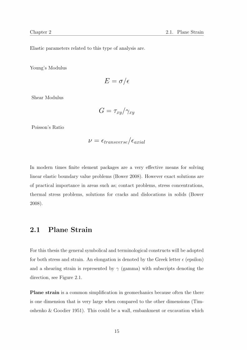
For this thesis the general symbolical and terminological constructs will be adopted
for both stress and strain. An elongation is denoted by the Greek letter ε (epsilon)
and a shearing strain is represented by γ (gamma) with subscripts denoting the
direction, see Figure 2.1.
Plane strain is a common simplification in geomechanics because often the there
is one dimension that is very large when compared to the other dimensions (Tim-
oshenko & Goodier 1951). This could be a wall, embankment or excavation which
15
Chapter 2 2.1. Plane Strain
is extremely long in comparison to its height and width, the assumption is that
the strain in the longitudinal direction is zero (Powrie 2004, pp.70). The principle
of plane strain may only be applied when there are no significant changes in cross
sectional dimensions or loadings.
For example taking the cross section of an extremely long embankment and the z
axis as the longitudinal direction; the z dimension is so large when compared to
the other dimensions any strain (a ratio of its deformed length over its original
length) will be so small that it can be deemed negligible and therefore εz, γxz and
γyz would be approximately equal to 0. The application of plane strain greatly
simplifies any subsequent stress analysis on the body (Powrie 2004, pp.70). See
Figure 2.1 for a diagrammatic representation of plane strain.
Figure 2.1: Plane Strain (Source: http://academic.uprm.edu/pcaceres/Courses/
MechMet/MET-2B.pdf
16
Chapter 2 2.2. Plane Stress
2.2 Plane Stress
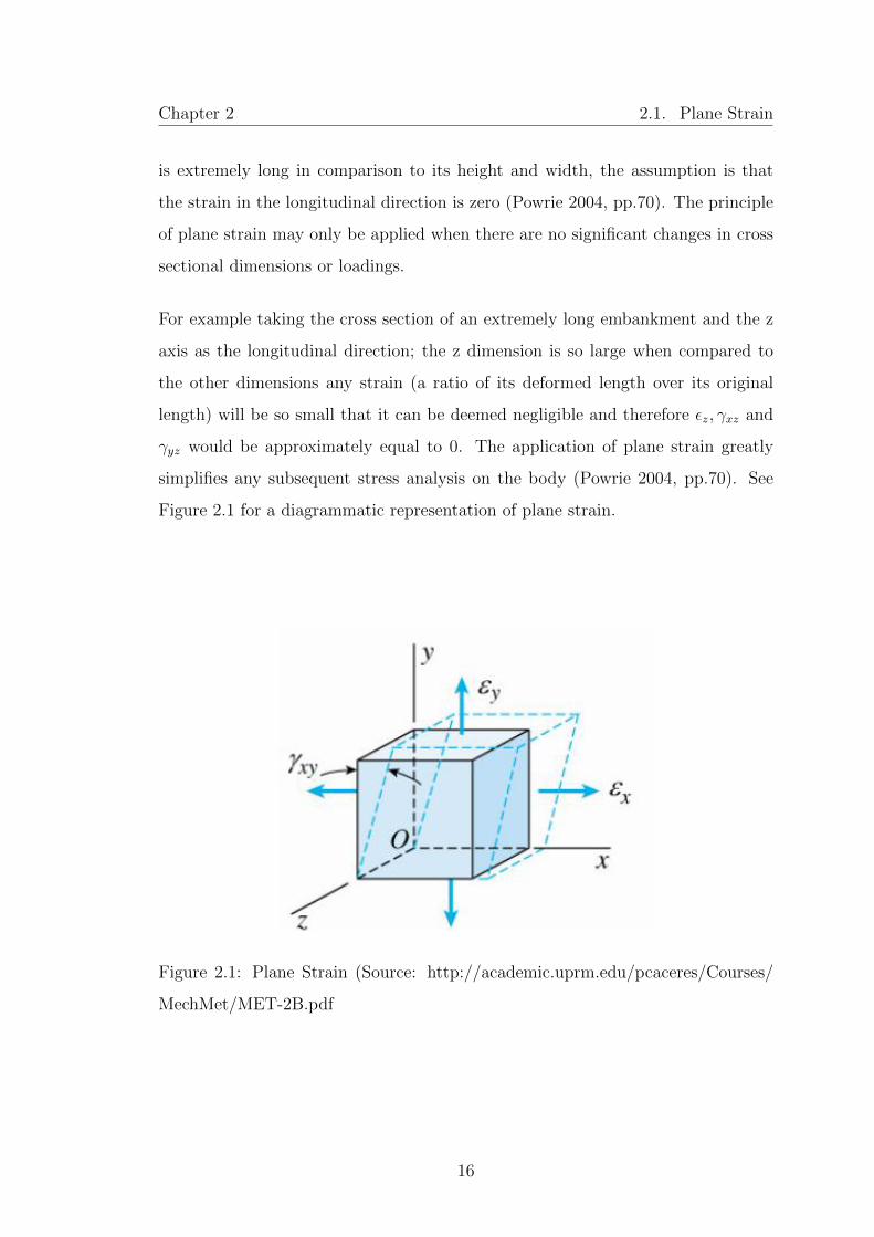
A stress that is normal to the plane is denoted by the Greek letter σ (sigma).
A stress which acts parallel to the plane is denoted by the Greek letter τ(tau).
Axial subscripts are used to denote the planar direction in which these stresses
act, for example a subscript of σx means a normal stress, acting parallel to the
x-axis (Timoshenko & Goodier 1951). For τxy the first letter indicates that the
stress is normal to the x axis and the second letter indicates that it is in the same
direction as the y axis.
Plane stress similarly to plane strain suggests the negligence or nullification of
normal and shear stress in one axial direction. Typically a state of plane stress
occurs when one dimension is very small relative to the others. A related example
could be the stresses on a thin plate submerged in soil media.
Figure 2.2: Plane Stress (Source: http://academic.uprm.edu/pcaceres/Courses/
MechMet/MET-2B.pdf)
In soil mechanics compressive stresses and strains are usually taken as positive and
shear stresses and associated strains which create a clockwise moment about an
17

Chapter 2 2.3. Axisymmetric Models
exterior point to the plane being considered will be taken as positive (Perloff &
Baron 1976, pp.55). These conventions will be adopted in this thesis.
2.3 Axisymmetric Models
Powrie (2004, pp.71) states that when stress and strain conditions on a plane
have rotational symmetry about the vertical axis it can be termed axisymmetric.
Like plain strain, when a body satisfies axisymmetry stress analysis is greatly
simplified. On occasions where a problem is restricted from featuring either of
these simplifications numerical solutions are usually required such as finite element
or finite difference analysis (Powrie 2004, pp.71).
Figure 2.3: Stress strain axisymmetry of a pile (Powrie 2004, pp.71).
In geomechanics this principle can typically be applied to circular subsurface ob-
jects. Axisymmetry is a convenience as it can provide a simplification of the rela-
tionships between variables. For example taking an axisymmetric loading around
the circumference of a circular tunnel simplifies the relationship between tunnel
18

Chapter 2 2.3. Axisymmetric Models
loading and spatial dimensions. Using the same example axisymmetric soil condi-
tions surrounding the tunnel would eliminate the significance of the location of the
cross section taken.
19
Chapter 3
Solutions for Stress in Soil Masses
and their Applications
3.1 Introduction
This chapter sets the foundation for the area of Geotechnical Engineering in which
this paper focuses, stress in soil masses. Three solutions for linear elasticity prob-
lems have been selected. The three solutions that have been selected are all closely
related yet are individualised in terms of their load placements. The first of the
solutions was developed by Lord Kelvin (1824-1907) a physicist and engineer, for a
point load acting within an infinite elastic mass. The second by Joseph Boussinesq
(1842-1929) a French physicist, for a point load acting on the surface of a linear
elastic semi-infinite mass. The third by Raymond D. Mindlin (1906-1987) for a
point load acting beneath the surface of a semi-infinite mass.
All three solutions assume a homogeneous, isotropic, elastic medium. A material
is said to be homogeneous when its physical properties are identical at all points
within its boundaries and it is said to be isotropic when the elastic properties
20
Chapter 3 3.2. Kelvin’s Solution
of the material are the same in all directions (Timoshenko & Goodier 1951). In
reality absolute homogeneity and isotropy are both unlikely but the assumptions
can still provide accurate results as long as the geometric dimensions of the body
under study are large enough so that internal inconsistencies may be averaged out
(Timoshenko & Goodier 1951). In Geomechanics any vast discrepancies in soil
properties would need to be taken into account.
3.2 Kelvin’s Solution
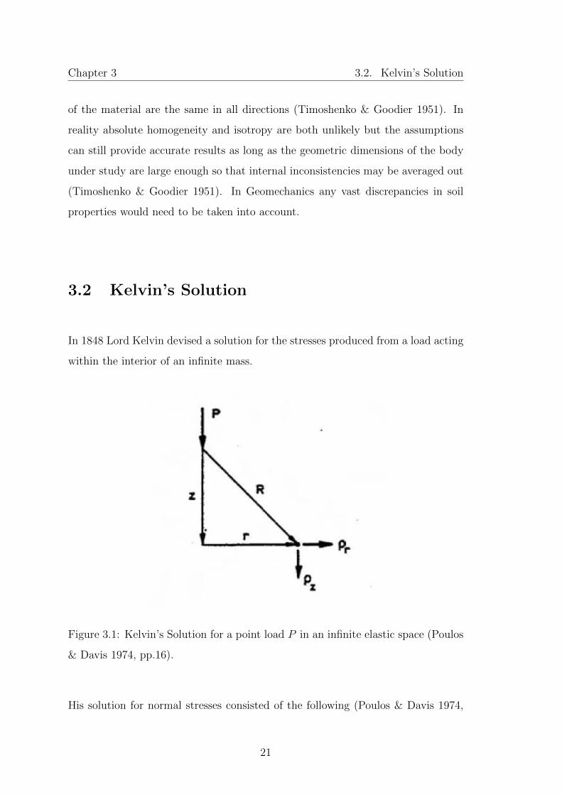
In 1848 Lord Kelvin devised a solution for the stresses produced from a load acting
within the interior of an infinite mass.
Figure 3.1: Kelvin’s Solution for a point load P in an infinite elastic space (Poulos
& Davis 1974, pp.16).
His solution for normal stresses consisted of the following (Poulos & Davis 1974,
21

Chapter 3 3.2. Kelvin’s Solution
pp.16).
σz =P
8π(1− ν)
[3z3
R5+
(1− 2ν)z
R3
](3.1)
σr =P
8π(1− ν)
z
R3
[−3r2
R2− (1− ν)
](3.2)
σθ = −P (1− 2ν)
8π(1− ν)
z
R3(3.3)
and for displacement,
ρz =P (1 + ν)
8π(1− ν)ER
[3− 4ν
z2
R2
](3.4)
ρr = − P (1 + ν)
8π(1− ν)E· rzR3
(3.5)
where subscripts r,z and θ indicate direction. θ is the circumferential direction,
perpendicular to both r and z
As Kelvin’s problem excludes a surface, the practical applications of this particular
solution are limited. Kelvin’s solution can be integrated to determine distributed
loads.
22

Chapter 3 3.3. Boussinesq’s Solution
3.3 Boussinesq’s Solution
In 1885 Boussinesq solved the problem involving a point load acting at the surface
of an elastic half space (a body of infinite depth and width, also known as a
semi-infinite domain) to find the stress and strains at any point within it (Powrie
2004, pp.336).
Figure 3.2: Boussinesq’s solution for a point load P acting at the surface of a
semi-infinite elastic space (Perloff & Baron 1976, pp.179).
Referring to the figure above, the Boussinesq solution consists of the following
equations for normal stress (Poulos & Davis 1974, pp.16).
σz =3Pz3
2πR5(3.6)
23

Chapter 3 3.4. Mindlin’s Solution
σr = − P
2πR2
[−3r2z
R3− (1− 2ν)R
R + z
](3.7)
σθ = −(1− 2ν)R
2πR2
[z
R− R
R + z
](3.8)
and for displacement,
ρz =P (1 + ν)
2πER
[2(1− ν) +
z2
R2
](3.9)
ρr =P (1 + ν)
2πER
[rz
R2− r(1− 2ν)
R + z
](3.10)
where subscripts r,z and θ indicate direction. θ is the circumferential direction,
perpendicular to both r and z. Due to the fact that many geotechnical engineering
tasks take place on the surface these equations are extremely useful. Like Kelvin’s
solution, Boussinesq’s equations can also be integrated to facilitate for line loads
and area loads.
3.4 Mindlin’s Solution
In 1936 Raymond D. Mindlin developed a solution of the three dimensional elastic-
ity equations for a homogeneous, isotropic, semi-infinite solid with a force acting
in its interior (Mindlin 1936).
Kelvin and Boussinesq had both reached fundamental results in this area prior to
Mindlin’s development. Both of their solutions had a range of practical uses, but
Mindlin still saw room for advancement. Mindlin described his paper as a solution
24
Chapter 3 3.4. Mindlin’s Solution
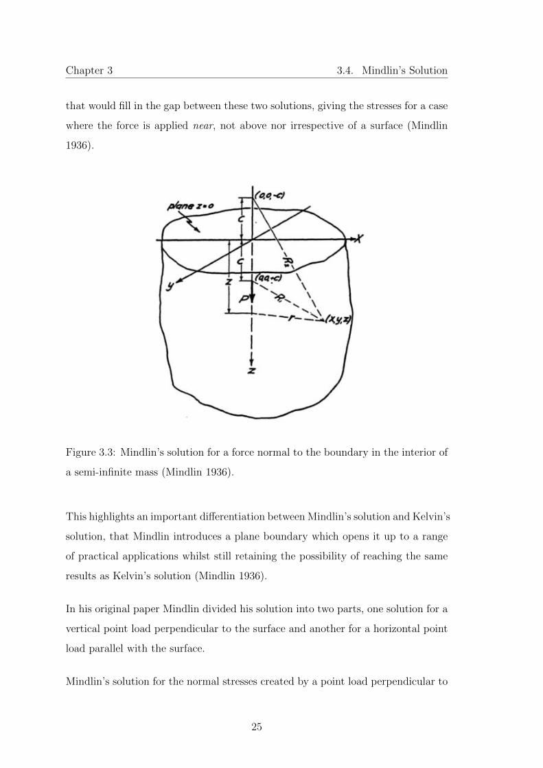
that would fill in the gap between these two solutions, giving the stresses for a case
where the force is applied near, not above nor irrespective of a surface (Mindlin
1936).
Figure 3.3: Mindlin’s solution for a force normal to the boundary in the interior of
a semi-infinite mass (Mindlin 1936).
This highlights an important differentiation between Mindlin’s solution and Kelvin’s
solution, that Mindlin introduces a plane boundary which opens it up to a range
of practical applications whilst still retaining the possibility of reaching the same
results as Kelvin’s solution (Mindlin 1936).
In his original paper Mindlin divided his solution into two parts, one solution for a
vertical point load perpendicular to the surface and another for a horizontal point
load parallel with the surface.
Mindlin’s solution for the normal stresses created by a point load perpendicular to
25

Chapter 3 3.4. Mindlin’s Solution
the surface involves the following equations (Poulos & Davis 1974, pp.16).
σx =− P
8π(1− ν)
[(1− 2ν)(z − c)
R31
− 3x2(z − c)R5
1
+(1− 2ν)[3(z − c)− 4ν(z + c)]
R32
− 3(3− 4ν)x2(z − c)− 6c(z + c)[(1− 2ν)z − 2νc]
R52
− 30cx2z(z + c)
R72
−(
4(1− ν)(1− 2ν)
R2(R2 + z + c)
)(1− x2
R2(R2 + z + c)− x2
R22
) ](3.11)
σy =− P
8π(1− ν)
[(1− 2ν)(z − c)
R31
− 3y2(z − c)R5
1
+(1− 2ν)[3(z − c)− 4ν(z + c)]
R32
− 3(3− 4ν)y2(z − c)− 6c(z + c)[(1− 2ν)z − 2νc]
R52
− 30cy2z(z + c)
R72
−(
4(1− ν)(1− 2ν)
R2(R2 + z + c)
)(1− y2
R2(R2 + z + c)− y2
R22
) ](3.12)
σz =− P
8π(1− ν)
[−(1− 2ν)(z − c)
R31
+(1− 2ν)(z − c)
R32
− 3(z − c)3
R51
− 3(3− 4ν)z(z + c)2 − 3c(z + c)(5z − c)R5
2
− 30cz(z + c)3
R72
] (3.13)
Furthermore noting axisymmetry for the case of vertical load, instead of two for-
mulae σx and σy, it can be exemplified by one formula σr.
σr =− P
8π(1− ν)
[(1− 2ν)(z − c)
R31
− (1− 2ν)(z + 7c)
R32
+4(1− ν)(1− 2ν)
R2(R2 + z + c)
− 3r2(z − c)R5
1
+6c(1− 2ν)(z + c)2 − 6c2(z + c)− 3(3− 4ν)r2(z − c)
R52
− 30cr2z(z + c)
R72
](3.14)
26

Chapter 3 3.5. Applications in Geotechnical Problems
and for displacement,
ρz =P
16πG(1− ν)
[3− 4ν
R1
+8(1− ν)2 − (3− 4ν)
R2
+(z − c)2
R31
+(3− 4ν)(z + c)2 − 2cz
R32
+6cz(z + c)2
R52
] (3.15)
ρr =Pr
16πG(1− ν)
[z − cR3
1
+(3− 4ν)(z − c)
R32
− 4(1− ν)(1− 2ν)
R2(R2 + z + c)
+6cz(z + c)
R52
(3.16)
Where,
r =√x2 + y2
R1 =√r2 + (z − c)2
R2 =√r2 + (z + c)2
3.5 Applications in Geotechnical Problems
This section provides a review of literature on the applications of closed form
Mindlin’s, Boussinesq’s and Kelvin’s solutions. There has been many numerical
methods developed referencing these solutions but as this thesis centres on ana-
lytical solutions these papers will not be reviewed. Additionally papers which in-
volve anisotropic or non-homogeneous media will not be considered as the solutions
discussed in this thesis are specifically formulated for an isotropic, homogeneous
medium.
27

Chapter 3 3.5. Applications in Geotechnical Problems
3.5.1 Applications in Piling
As piles are generally inserted into the ground for the support and stability of
structures they are responsible for the transmission of heavy loadings into the
soil beneath. Pile analysis is a major civil engineering problem and one in which
elasticity theory has been used as a method to analyse piles and pile groups.
In their 1971 paper Butterfield and Banerjee performed an elastic analysis of rigid
and compressible piles and pile groups based on the use of Mindlin’s solution in
a homogeneous isotropic medium. Through integration of Mindlin’s point load
solutions they were able to obtain insight into the relationships between certain
variables within the system.
The study observed the effect of variations in the ratio of pile length to pile diame-
ter, the ratio of modulus of elasticity of the pile to shear modulus of the medium of
which it is situated and the effect that enlarging the base has on the load displace-
ment characteristics of singular piles. When Butterfield and Banerjee compared
their results with published approximate solutions and laboratory tests they found
them to be close enough to warrant the use of their solution for the calculation of
pile group settlement ratios and the prediction of pile group behaviour based on
single pile load displacement data.
Comparisons between Mindlin’s solution and Boussinesq’s solution for the stresses
resulting from distributed subsurface loadings (triangular and rectangular) were
studied by Geddes in 1966. While Mindlin’s solution was applied successfully it
was found that if Boussinesq’s solution was adopted significant overestimates were
produced (Geddes 1969). This is because Boussinesq’s solution is not designed for
subsurface loading.
Geddes (1969) modified the Boussinesq solution to include subsurface loading cater-
ing for vertical skin friction forces in piles. A limitation being that it does not
28

Chapter 3 3.5. Applications in Geotechnical Problems
take into account the presence of overburden loading as the solution is based on
the Boussinesq solution which acts at the surface. Therefore in general Geddes’
solution will produce overestimates for stress. As the solution was intended for
approximation purposes this inaccuracy is only a minor limitation.
Tian-quan (1981) detailed pile analysis on both rigid and compressible piles by
using two simple integral equation methods. The first consisting of a horizontal
Mindlin force distributed along an axis combined with a Boussinesq point force
and the second consisting of a a distributed vertical Mindlin force (Tian-quan
1981). The paper was able to transform a three dimensional problem into a one
dimensional Fredholm integral equation of the first kind.
3.5.2 Applications in Anchoring
Similarly to piling, Earth or ground anchors are a foundation providing support
and stability for certain structures. Anchors are tensile members as there are usu-
ally tensile forces involved, anchoring in place whilst undergoing uplift forces or
horizontal pull out forces (Altun, Karakan and Caglar Tuna 2013). Sub-surface
loadings such as these open up anchoring problems to analysis via Mindlin’s so-
lution. Furthermore some anchors provide an opposite force acting at the surface
compressing the soil, such as a plate, in this case Boussinesq’s solution may be
used. Having both tensile and compressive forces working together can improve
the support offered by the anchor so for some designs it may be preferable to have
both, thus it may be possible to analyse an anchor system involving a combination
of both Mindlin’s and Boussinesq’s solutions.
Many of the following applications are more related to contact mechanics which
strays somewhat further away from the more traditional civil and geotechnical
engineering applications discussed in other sections. Nonetheless they represent
an important and well researched area on the application of the selected elasticity
29

Chapter 3 3.5. Applications in Geotechnical Problems
solutions whilst often containing problems in relation to ground anchors.
Selvadurai (1979) formulated a closed form solution based on Mindlin’s equations
for the displacement experienced by a rigid circular plate connected to a ground
anchor. The problem involved an isotropic, elastic half-space subject to axisym-
metric internal and external loads (see Figure 3.4) (Selvadurai 1979). The analysis
contained a variety of distributed loading cases, constant, linear and parabolic; ne-
glecting any effects of friction (Selvadurai 1979). The paper also suggests that this
particular problem has useful connections with rock anchoring and in situ testing.
Figure 3.4: Selvadurai’s anchored rigid circular plate (Selvadurai 1979).
In their 2013 research paper, Altun, Karakan and Caglar Tuna followed on from
Salvarudai’s 1979 work, analysing the load-displacement relationship for a rigid
ground anchored circular plate using Mindlin’s solution. The effects of anchor
length, anchor depth and the type of load distribution has on the load-displacement
relationship was also observed (Altun et al. 2013).
For verification purposes Altun, Karkan and Caglar Tuna also undertook FEM
30

Chapter 3 3.5. Applications in Geotechnical Problems
(Finite Element Method) analysis and compared it with their analytical results.
It was found that the two methods did not agree well for Mindlin’s problem and
that the reasoning for this was due to discrepancies in the solution procedures
and the material properties assigned in each method (Altun et al. 2013). In spite
of these disagreements it is suggested that the analytical solutions to determine
anchor displacements may still be applicable as long as it is in the case of an ideal
soil and the elastic parameters are determined correctly (Altun et al. 2013).
3.5.3 Applications in Tunnelling
Tunnels are often a part of engineering projects in areas such as transport, public
health and mining engineering. Tunnels have been subjected to research in which
elastic analysis including Mindlin’s solution has been performed in order to pre-
dict nearby soil displacements and to examine the effect of stresses on places of
interest in the proximity. Such analysis could theoretically be performed on other
underground excavations such as caverns or shafts.
Zhang et al. (2013) utilised a semi-analytical approach for geotechnical tunnel anal-
ysis where the tunnel was assumed as an elastic beam. An integrated Boussinesq’s
solution was used to determine the distributed soil stresses and tunnel displacement
induced by an adjacent excavation. Additionally, through integration of Mindlin’s
solution, Zhang et al. (2013) was able to estimate the resistance of a tunnel. Their
work is founded on the contemporary challenges of incorporating metro systems
into urban areas, as the interaction between underground structures and existing
tunnels represents a significant safety concern.
Among the results were the effects of different factors on heave displacement (heav-
ing of a tunnel happens due to the rebound of soil when adjacent soil is exca-
vated), these included excavation area, relative distance and construction proce-
dure (Zhang et al. 2013). A good conformity was found when the displacement
31

Chapter 3 3.5. Applications in Geotechnical Problems
results were verified against the field measurements for deep excavations above
metro tunnels (Zhang et al. 2013).
Among the limitations of the semi-analytical method, Zhang et al. (2013) noted
that it was best used for quick assessment of tunnel displacement and for higher
accuracy numerical analysis should be utilised. Additionally clarification is needed
as to whether or not this method may be applied when soil properties change with
time, take for example soft clays (Zhang et al. 2013).
Chow (1994, p.16) used Mindlin’s solution for finding the surface displacement in a
shallow tunneling problem (see figure 3.5). Chow postulated that the total vertical
displacement at point O could be found through integrating equation 3.15 along
the y axis from −∞ to +∞.
Figure 3.5: Tunnel problem (Chow 1994, pp.16).
In the paper a solution was reached which could not be evaluated analytically (and
hence exact surface displacements could not be found). After reformulating the
approach, relative surface displacements were found by comparing displacements
at two points (Chow 1994).
32

Chapter 3 3.5. Applications in Geotechnical Problems
3.5.4 Applications in Contact Mechanics
Mindlin’s solution has been used in a wide range of research in contact problems.
Selvadurai (2001) analysed via Mindlin’s problem for a half space bonded with a
thin plate of infinite extent at the surface subject to an axisymmetric load. The aim
of such an analysis is to identify and develop integral expressions for the influence
a Mindlin force has on deflections and moments inside the plate (Selvadurai 2001).
Rahman and Newaz (2000) modelled a Boussinesq type solution for a load acting
at the surface of an isotropic half-space in which the surface had been coated with
a thin soft film. The applications for this research are more tuned to mechanical
areas with such examples given as magnetic layer protection for hard disk files
and thermal protection in aerospace design (Rahman & Newaz 2000). In general,
the results may be useful in determining solutions for frictionless contact problems
where the surface is reinforced by thin coatings (Rahman & Newaz 2000).
3.5.5 General Research and Applications
Sun et al. (2013) developed an extended, integrated form of Mindlin’s displacement
equations to find displacements at an arbitrary point induced by horizontally or
vertically distributed loading acting normally or tangentially. The results were
compared and found to correlate well with existing literature in the area (Sun et
al. 2013).
Sun et al. (2013) indicate that the formulae can be used to understand displace-
ment fields around embedded structures in practical situations and furthermore
may be useful in the development of future computer programs in the area.
Basile (2002) presented the integration for a singular Mindlin displacement so-
lution over a cylindrical surface. The derivation of the equation is presented in
33

Chapter 3 3.5. Applications in Geotechnical Problems
full. Such analytical solutions are helpful in reducing computational resources
required in certain analyses (Basile 2002). Likewise Douglas and Davis (1964) in-
tegrated Mindlin’s horizontal displacement equations in order to attain values for
the displacement and rotation of a vertically buried footing subject to moment
and horizontal loadings. Ultimately this solution was used in a numerical method,
however this paper is still somewhat relevant to this thesis as the integration of
Mindlin’s solution is displayed.
Figure 3.6: Dominguez (1966) detailed how the stress due to a uniform distributed
load over the area of the shaded section above could be found through integration.
Dominguez (1966) showed the steps involved in integrating Boussineq’s equation
for normal stress along the x,y,z axes for both horizontal and vertical loadings over
a radial area (see Figure 3.6). Dominguez’s expressions are also fairly flexible as
can be seen from Figure 3.6 in that it allows the disregard of certain segments of
the circle based on input radius (ρ) and the angular span (φ).
34

Chapter 3 3.5. Applications in Geotechnical Problems
The expressions developed by Dominguez could be further built upon or used in
subsequent analysis. Dominguez’s integrated Boussinesq’s solution is used as a
calculation check in Chapter 4.
Acknowledging the previously published results by Poulos Davis (1974), Vaziri et
al. (1982) produced the integrated forms of Mindlin’s displacement equations in
both the x and z directions for both horizontal and vertical loadings. Through
integrating these equations Vaziri et al. produced the expressions for the dis-
placements due to a uniform shear stress as well as displacements produced by a
uniformly distributed pressure. The motivation behind this research was to assist
in the development of a computer program for retaining walls (Vaziri et al. 1982).
Vaziri et al. (1982) validated the integrated solutions using a variety of techniques
which found them to be correct.
3.5.6 Summary of Applications
Overall there is by no means a large amount of literature on this topic area. The lit-
erature reviewed in this section makes heavy use of both Boussinesq’s and Mindlin’s
solutions over a variety of applications mainly piling, anchoring and tunnelling. As
these were the main areas of application, they will serve as first preference when
exploring possible new analytical calculations within them.
It is also worth noting the absence of Kelvin’s solution in the literature. The
reason for this is most likely due to the limited practical value of Kelvin’s solu-
tion. Nonetheless it is still an important solution as it set the foundation for both
Boussinesq and Mindlin to build upon in the formulation of their own solutions.
35
Chapter 4
Circular Sub-Surface Loading
4.1 Introduction
Now that the abilities and possible areas of application of the chosen solutions have
been identified this chapter serves as an exploration into some of the possible appli-
cations which have not yet been covered in literature. The calculations presented
here can further undergo subsequent analysis against their numerical counterparts
in order to determine their true value, both in general and due to its analytical
form.
4.2 Integration of Mindlin’s Solution for a Uni-
formly Distributed Sub-Surface Circular Load
While much of the covered literature (Geddes 1966, Vaziri et al. 1982, Basile 2002,
Zhang et al. 2013, Douglas Davis 1964) included developed integrated Mindlin’s
solutions for sub-surface loadings; these publications do not all explicitly show
36

Chapter 4 4.2. Integration of Mindlin’s Solution
the integration process nor state the fully integrated solution. Additionally there
appears to be an emphasis on integrating Mindlin’s displacement equations whilst
the integration of Mindlin’s original stress equations appear to have not yet been
published. Geddes (1966) did include and show the integration of Mindlin’s stress
equations however it was a modified version to cater for numerical applications.
This section contains the integration of the original normal stress equation devel-
oped by Mindlin as well as a possible ways in which it can be applied.
Figure 4.1 illustrates a potential area of exploration for the integrated form of
Mindlin’s equation for normal stress generated by a vertical force.
Figure 4.1: A uniformly distributed vertical circular loading beneath the surface
(x-y plane).
37

Chapter 4 4.2. Integration of Mindlin’s Solution
Taking Mindlin’s equation for normal stress in the z direction,
σz =− P
8π(1− ν)
[−(1− 2ν)(z − c)
R31
+(1− 2ν)(z − c)
R32
− 3(z − c)3
R51
− 3(3− 4ν)z(z + c)2 − 3c(z + c)(5z − c)R5
2
− 30cz(z + c)3
R72
] (4.1)
and integrating with respect to r and integrating again with respect to θ (angle in
radians), we can find σz induced by a uniformly loaded circular area, with a load
per unit area of q and a radius of R,
σz =
∫ 2π
0
∫ R
0
−q · r · dr · dθ8π(1− ν)
[−(1− 2ν)(z − c)
R31
+(1− 2ν)(z − c)
R32
− 3(z − c)3
R51
− 3(3− 4ν)z(z + c)2 − 3c(z + c)(5z − c)R5
2
− 30cz(z + c)3
R72
](4.2)
σz =− q
8π(1− ν)
∫ 2π
0
dθ
∫ R
0
r · dr[−(1− 2ν)(z − c)
R31
+(1− 2ν)(z − c)
R32
− 3(z − c)3
R51
− 3(3− 4ν)z(z + c)2 − 3c(z + c)(5z − c)R5
2
− 30cz(z + c)3
R72
](4.3)
Remembering,
R1 =√r2 + (z − c)2
R2 =√r2 + (z + c)2
38
Chapter 4 4.2. Integration of Mindlin’s Solution
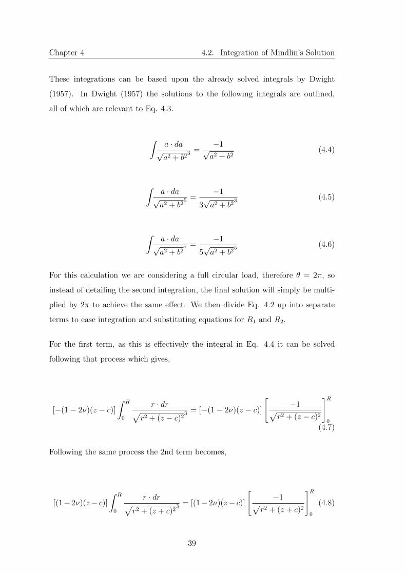
These integrations can be based upon the already solved integrals by Dwight
(1957). In Dwight (1957) the solutions to the following integrals are outlined,
all of which are relevant to Eq. 4.3.
∫a · da√a2 + b2
3 =−1√a2 + b2
(4.4)
∫a · da√a2 + b2
5 =−1
3√a2 + b2
3 (4.5)
∫a · da√a2 + b2
7 =−1
5√a2 + b2
5 (4.6)
For this calculation we are considering a full circular load, therefore θ = 2π, so
instead of detailing the second integration, the final solution will simply be multi-
plied by 2π to achieve the same effect. We then divide Eq. 4.2 up into separate
terms to ease integration and substituting equations for R1 and R2.
For the first term, as this is effectively the integral in Eq. 4.4 it can be solved
following that process which gives,
[−(1− 2ν)(z − c)]∫ R
0
r · dr√r2 + (z − c)23
= [−(1− 2ν)(z − c)]
[−1√
r2 + (z − c)2
]R0
(4.7)
Following the same process the 2nd term becomes,
[(1− 2ν)(z− c)]∫ R
0
r · dr√r2 + (z + c)2
3 = [(1− 2ν)(z− c)]
[−1√
r2 + (z + c)2
]R0
(4.8)
39
Chapter 4 4.2. Integration of Mindlin’s Solution
Integrating the 3rd term with assistance from equation 4.5, results in
[−3(z − c)3]∫ R
0
r · dr√r2 + (z − c)25
= −3(z − c)3[
−1
3√r2 + (z − c)23
]R0
(4.9)
Integrating the 4th term with assistance from equation 4.5, results in
−m∫ R
0
r · dr√r2 + (z + c)2
5 = −m
[−1
3√r2 + (z + c)2
3
]R0
(4.10)
where
m = 3(3− 4ν)z(z + c)2 − 3c(z + c)(5z − c)
Integrating the 5th term with assistance from equation 4.6, results in
−30cz(z + c)3∫ R
0
r · dr√r2 + (z + c)2
7 = −30cz(z + c)3
[−1
5√r2 + (z + c)2
5
]R0
(4.11)
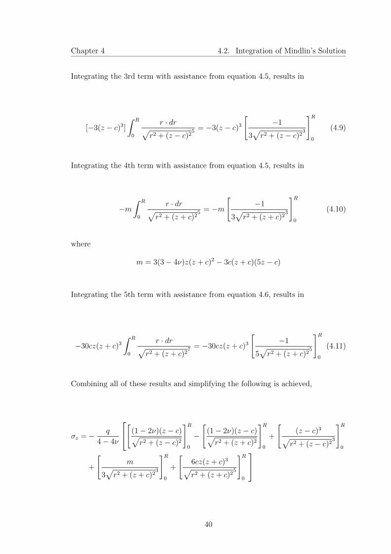
Combining all of these results and simplifying the following is achieved,
σz =− q
4− 4ν
[(1− 2ν)(z − c)√r2 + (z − c)2
]R0
−
[(1− 2ν)(z − c)√r2 + (z + c)2
]R0
+
[(z − c)3√
r2 + (z − c)23
]R0
+
[m
3√r2 + (z + c)2
3
]R0
+
[6cz(z + c)3√r2 + (z + c)2
5
]R0
40

Chapter 4 4.2. Integration of Mindlin’s Solution
Finally we obtain
σz =− q
4− 4ν
[[(1− 2ν)(z − c)√R2 + (z − c)2
]−
[(1− 2ν)(z − c)√
(z − c)2
]−
[(1− 2ν)(z − c)√R2 + (z + c)2
]
+
[(1− 2ν)(z − c)√
(z + c)2
]+
[(z − c)3√
R2 + (z − c)23
]−
[(z − c)3√(z − c)23
]
+
[m
3√R2 + (z + c)2
3
]−
[m
3√
(z + c)23
]+
[6cz(z + c)3√R2 + (z + c)2
5
]−
[6cz(z + c)3√
(z + c)25
] (4.12)
where
m = 3(3− 4ν)z(z + c)2 − 3c(z + c)(5z − c)
41

Chapter 4 4.2. Integration of Mindlin’s Solution
4.2.1 Comparing Integrated Mindlin’s and Boussinesq’s So-
lutions
As a preliminary exercise a comparison will be made between the integrated Mindlin’s
solution developed previously and integrated forms of Boussinesq’s equation for the
same parameter encountered in the literature.
Mindlin’s solution is developed exclusively for sub-surface loading, this section
looks at the effectiveness of Mindlin’s solution if the value of c were reduced to 0
as to imply the loading is at the surface. Furthermore this exercise will validate
whether or not Mindlin’s solution has been correctly integrated in Eq. 4.12.
Take c = 0 m (so that the load acts at the surface) therefore,
m = 3(3− 4ν)z(z + c)2 − 3c(z + c)(5z − c) = 3(3− 4ν)z(z)2 − 0 = 3z3(3− 4ν)
substituting these into Eq. 4.12 gives,
σz =− q
4− 4ν
[ z(1− 2ν)√R2 + z2
]−[z(1− 2ν)√R2 + z2
]+
[z(1− 2ν)√
z2
]−[z(1− 2ν)√
z2
]
+
[z3
√R2 + z2
3
]−
[z3√z2
3
]+
[3z3(3− 4ν)
3√R2 + z2
3
]−
[3z3(3− 4ν)
3√z2
3
]+ 0
σz =− q
4− 4ν
[[z3
√R2 + z2
3
]− 1 +
[z3(3− 4ν)√R2 + z2
3
]− (3− 4ν)
]
σz = − q
4− 4ν
[[z3
√R2 + z2
3
]+
[z3(3− 4ν)√R2 + z2
3
]− (4− 4ν)
]
42
Chapter 4 4.2. Integration of Mindlin’s Solution
σz = − q
4− 4ν
[z3(4− 4ν)
(R2 + z2)3/2− (4− 4ν)
]
σz =q(4− 4ν)
(4− 4ν)− qz3(4− 4ν)
(4− 4ν)(R2 + z2)3/2
σz = q
(1− z3
(R2 + z2)3/2
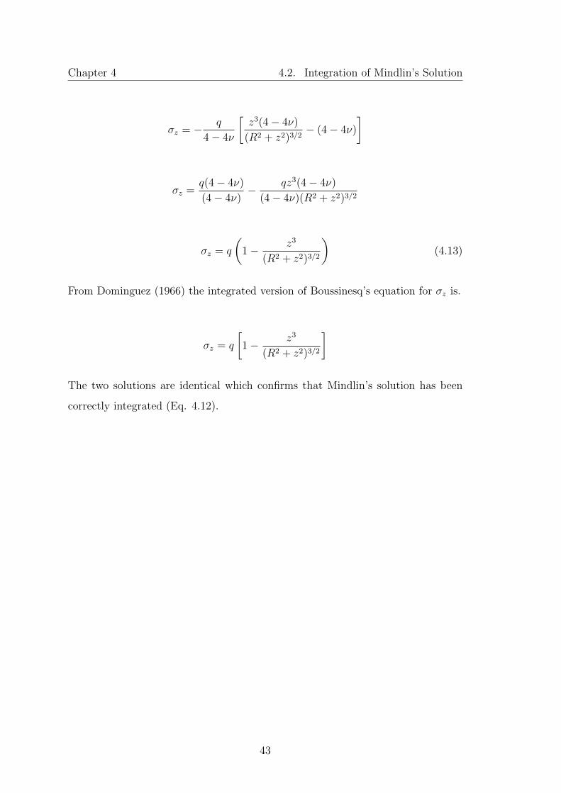
)(4.13)
From Dominguez (1966) the integrated version of Boussinesq’s equation for σz is.
σz = q
[1− z3
(R2 + z2)3/2
]
The two solutions are identical which confirms that Mindlin’s solution has been
correctly integrated (Eq. 4.12).
43

Chapter 5
Exploring the Applications of the
Integrated Mindlin’s Solution
This section explores some possible applications for the integrated Mindlin’s solu-
tion developed earlier (Eq. 4.12).
5.1 Mindlin Based Influence Chart
A Mindlin-based influence chart would offer advantages such as quick approxima-
tion, the ability to obtain values for irregular shaped loadings and easier calcula-
tion of stresses that are offset (do not lie directly beneath the center of the circular
loading). Such charts do not appear to exist for Mindlin’s solution though have
been developed for Boussinessq’s solution, namely Newmark’s chart developed by
Nathan Newmark in 1942 (Das & Sobhan 2010).
Noting the likeness between the integrated Mindlin’s solution (Eq. 4.12) and the
integrated Boussinesq’s solution for normal stress induced by a vertical load an at-
44

Chapter 5 5.1. Mindlin Based Influence Chart
tempt was made to develop an influence chart for Mindlin’s solution similar to that
of Newmark’s influence chart for Boussinesq’s solution. Newmark’s influence chart
is of great practical value due to its versatility, efficiency and useful approximation
capabilities.
In order to develop a chart similar to that of Newmark’s several variables had to
be taken as constants, namely, poisson’s ratio ν and the ratio c/z, where c is the
depth from the surface to the loaded area and z is the depth of the point of interest.
If these constants were taken as variables the values used to generate the chart
would not correlate and the chart would be useless. A trial and error approach was
undertaken by inputting different values of R into Eq. 4.12 to obtain predetermined
incremental values of σzq
. The same inputs used to generate Newmark’s chart were
targeted. Figure 5.1 shows the table of these results for c/z = 0.3 and ν = 0.3.
Newmark’s chart represents a special case of these charts with c/z = 0.
Figure 5.1: Table of values for creation of Newmark style Mindlin based influence
chart. c/z = 0.3 and ν=0.3.
Like in Newmark’s chart values of R/z were then used as the radii for the circles in
Figure 5.2. Again like Newmark’s chart the circles are dissected by evenly spaced
angular lines, the influence value is obtained by 1/N , where N is the number
of elements on the chart and the length of line AB represents the unit length
45

Chapter 5 5.1. Mindlin Based Influence Chart
R/z = 1(Das & Sobhan 2010).
Figure 5.2: The developed Mindlin based influence chart for c/z = 0.3 and ν = 0.3.
Two tests were performed to validate the accuracy of Figure 5.2 using the same
equation as Newmark’s chart (Das & Sobhan 2010, pp.344).
σz = (IV )qM (5.1)
where, IV is the influence value, q is the area load and M is the number of elements
covered by the area when placed on the chart. The diagrammatic components of
the following tests are located in Appendix B.
46

Chapter 5 5.1. Mindlin Based Influence Chart
TEST 1
z = 10m
c = 3m
R = 5m
q = 150kN
which gives 66 elements on chart therefore,
σz = 0.005 · 66 · 150 = 49.5 kN/m2
The above values when substitued into Mindlin’s solution gives σz = 50.08 kN/m2
error = 1.158%
Therefore, a good agreement was found and the chart can be deemed accurate.
TEST 2
z = 8m
c = 3m
R = 2m
q = 150kN
which gives 23 elements on chart therefore,
σz = 0.005 · 23 · 150 = 17.25 kN/m2
The above values when substituted into Mindlin’s solution gives σz = 18.04 kN/m2
error = 4.38% This error is much higher than test 1, which shows the chart not
useful for cz6= 0.3
47
Chapter 5 5.2. Stress Estimation In Bi-Loaded Anchors
5.1.1 Limitations
Although this chart can provide a quick and accurate approximation, the concept
of a Mindlin’s solution-based influence chart is of little practical value overall due
to the many variables which must maintain a constant value for the chart to be
produced. Therefore a different chart must be produced depending on different
values of c/z and ν. Further simplification was investigated with the aim to achieve
a pair of charts or graphs with one similar to Figure 5.2 and another that would
give a different scale to be utilised in conjunction with the other based off of ν
and cz. However due to the complexity of the integrated Mindlin’s solution (Eq.
4.12), this task was deemed too difficult to achieve with questions over its general
possibility.
Therefore even though a Mindlin-based influence chart was successfully created, it
serves little practical value due to the need to generate a great number of charts
for a great number of situations which would be very time consuming.
5.2 Stress Estimation In Bi-Loaded Anchors
Having reached severe limitations with the Mindlin based influence chart in the
previous section the need to find an useful application for Eq. 4.12 remained.
Investigations into applications for which the circular subsurface loading equation
could be applied were undertaken with a preference that it have practical relativity.
It was decided that the solution could obtain useful results if applied to a simpli-
fied anchor system. Recognition that both Boussinesq’s and Mindlin’s solutions
are mathematically compatible and therefore combinationally possible, provided
a particular avenue of intrigue. A bi-loaded anchor system, one of which that
contained two loads, a surface load representable by Boussinesq’s solution, and a
subsurface load expressible by that of Mindlin’s solution was explored.
48

Chapter 5 5.2. Stress Estimation In Bi-Loaded Anchors
It was deemed that Eq. 4.12 may be an effective way to determine the amount of
loading required to eliminate tension in bi-loaded ground anchors. Figure 5.3 shows
the loading conditions for a bi-loaded ground anchor analysed in this thesis. Such
an anchor is commonly used in practice as the compressive force applied at the
surface further strengthens the anchorage. Given a uniformly distributed circular
surface and sub-surface load it is possible to then combine both Eqs. 4.12 and
4.13 (Mindlin’s and Boussinesq’s respectively) to formulate what surface loading
is required to nullify tensile stresses directly beneath the sub-surface load. It is an
important area of examination with practical significance as tensile stresses in soil
beneath the ground anchor would ultimately mean failure due to the poor tensile
capacity of soil.
Both Boussinesq’s and Mindlin’s solutions are particularly compatible in this cir-
cumstance as the value of z would be the same for both. As a negative stress
indicates a tensile stress, combining Eqs. 4.12 and 4.13, equating to zero and then
solving for the circular surface load would give the load needed at the surface to
nullify tensile stresses beneath the anchor.
49

Chapter 5 5.2. Stress Estimation In Bi-Loaded Anchors
Figure 5.3: An isometric representation of a bi-loaded anchor system with a Boussi-
nesq load acting on the surface plane and a Mindlin load acting on a parallel
sub-surface plane a distance of c below.
50

Chapter 5 5.2. Stress Estimation In Bi-Loaded Anchors
5.2.1 Example
This example displays the steps involved in finding the required qB to nullify tensile
stresses, although as seen in the next section this is not the penultimate solution
in doing so.
Taking z = c as this is where the maximum tensile stresses would reside.
ν = 0.25
z = c = 5m
RB = 1.2m
RM = 1.2m
qM = 200 kN/m2
qB =?
Taking the integrated Mindlin solution
σz =− qM4− 4ν
[[(1− 2ν)(z − c)√R2M + (z − c)2
]−
[(1− 2ν)(z − c)√
(z − c)2
]−
[(1− 2ν)(z − c)√R2M + (z + c)2
]
+
[(1− 2ν)(z − c)√
(z + c)2
]+
[(z − c)3√
R2M + (z − c)23
]−
[(z − c)3√(z − c)23
]
+
[m
3√R2M + (z + c)2
3
]−
[m
3√
(z + c)23
]+
[6cz(z + c)3√R2M + (z + c)2
5
]−
[6cz(z + c)3√
(z + c)25
] where
m = 3(3− 4ν)z(z + c)2 − 3c(z + c)(5z − c)
and the integrated Boussinesq solution
σz = qB
[1− z3
(R2B + z2)3/2
]
substituting in the values we get
51

Chapter 5 5.2. Stress Estimation In Bi-Loaded Anchors
m = 3(3− 4× 0.25)5(5 + 5)2 − 3× 5(5 + 5)(5× 5− 5) = 3000− 3000 = 0
qB
[1− 53
(0.82 + 52)3/2
]=
200
4− 4× 0.25
[[−(1− 2× 0.25)− 1 +
[6× 5× 5(5 + 5)3√
1.22 + (5 + 5)25
]
−
[6× 5× 5(5 + 5)3√
(5 + 5)25
]
0.08057qB = 66.6667 [−0.5− 1 + 1.4473− 1.5]
0.08057qB = 66.6667×−1.5527
qB =−103.5133
0.08057
qB = −1284.8kN/m2
5.2.2 Graphical Approach for a Bi-Loaded Anchor System
Having reached difficulties in developing an effective Newmark style influence chart
for Mindlin’s solution, an attempt was made to create a graph which was also based
on influence factors (σz/q) that could allow an easy comparison between integrated
Mindlin’s and Boussinesq’s solutions. The plots in this section were developed using
the computer program MATLAB, the code for which can be found in Appendix
C. Figure 5.4 shows the influence factor curves for multiple values of ν and for
Boussinesq’s equation for an increasing ratio R/z.
Discussion of Figures 5.4, 5.5 and 5.6
An interesting thing to note is that when z = c and R = 0, the integrated Mindlin’s
solution is equal to 12. This emulates what happens when c approaches ∞ where
Mindlin’s solution becomes reminiscent Kelvin’s solution. Figure 5.4 can be used
for estimating the R/z required for the Boussinesq load to nullify the maximum
52

Chapter 5 5.2. Stress Estimation In Bi-Loaded Anchors
tensile stresses caused by the subsurface Mindlin load (which is at the point of
loading z = c). The figure also conveys a strange result, the curves for ν = 0.5
and ν = 0.4 gives an I > 1 at a certain range of R/z with a maximum of 1.009
occurring at R/z = 4 on the ν = 0.5 curve. Such a result should be impossible as
the maximum difference between compressive and tensile influence factors should
be exactly equal to 1 at z = c. The point located infinitesimally above c+, should
emanate a compressive stress and the point infinitesimally below c−, a tensile stress
given the load is acting directly upwards, normal to the surface. An influence factor
of > 1 negates such a necessity. The cause of this anomaly is unknown but it could
represent a problem or limitation of Mindlin’s solution.
Following the curve for ν = 0.5, when R/z = 1 the influence factor is 0.75 and from
the Boussinesq curve, the surface loading would require an R/z = 1.233 to achieve
the same influence factor and counter this. Therefore from this information we
know that the RB would need to be altered in Eq. 4.13, see below.
σz = q
(1− z3
((1.233RB)2 + z2)3/2
)
Doing so, arrives at Figure 5.6 which indicates that tensile stresses are still present.
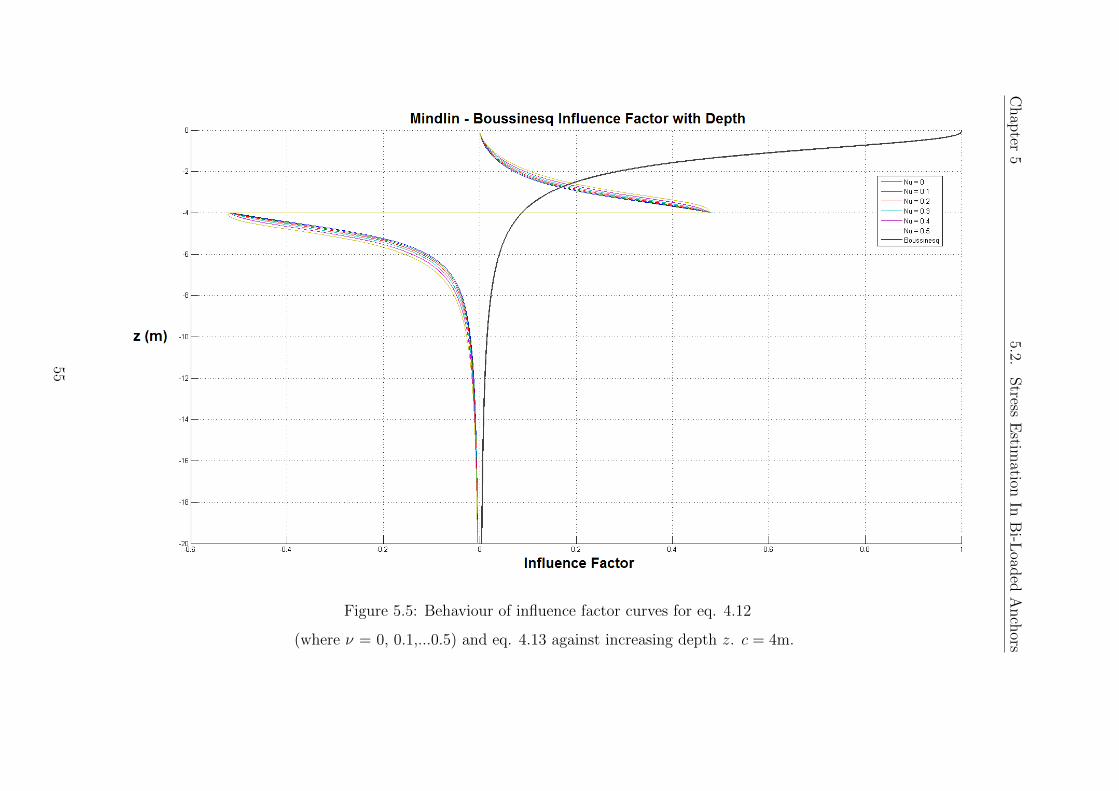
An explanation for this presence can be obtained by observing Figure 5.5 which
exhibits the decline in stress caused by both loads as the depth increases. This
element is a limitation of Figure 5.4 as it does not take into account the weakening
intensity of the Boussinesq surface load as the depth z, increases. So the above
equation results in Figure 5.6 where tensile stresses are nullified at the point of
loading (σz = 0 at c−) but as the depth z, increases below this point there is a
zone where the subsurface Mindlin loading has much more of an influence on the
stress conditions than Boussinesq’s surface load does and hence tensile stresses
remain. It is possible to develop a graphical relationship between the surface and
subsurface loadings that nullify not only the maximum, but all tensile stresses,
this is presented in the next section.
53

Chap
ter5
5.2.Stress
Estim
ationIn
Bi-L
oaded
Anch
ors
Figure 5.4: Influence factor curves for eq. 4.12
with ν = 0, 0.1,...0.5 and eq. 4.13.
54
Chap
ter5
5.2.Stress
Estim
ationIn
Bi-L
oaded
Anch
ors
Figure 5.5: Behaviour of influence factor curves for eq. 4.12
(where ν = 0, 0.1,...0.5) and eq. 4.13 against increasing depth z. c = 4m.
55

Chap
ter5
5.2.Stress
Estim
ationIn
Bi-L
oaded
Anch
ors
Figure 5.6: Behaviour of a combined Mindlin - Boussinesq influence factor curve against increasing depth z. c = 4m.
56
Chapter 5 5.2. Stress Estimation In Bi-Loaded Anchors
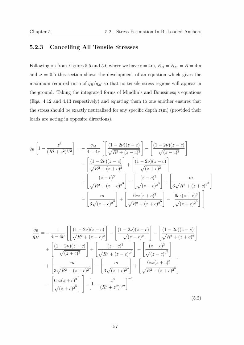
5.2.3 Cancelling All Tensile Stresses
Following on from Figures 5.5 and 5.6 where we have c = 4m, RB = RM = R = 4m
and ν = 0.5 this section shows the development of an equation which gives the
maximum required ratio of qB/qM so that no tensile stress regions will appear in
the ground. Taking the integrated forms of Mindlin’s and Boussinesq’s equations
(Eqs. 4.12 and 4.13 respectively) and equating them to one another ensures that
the stress should be exactly neutralized for any specific depth z(m) (provided their
loads are acting in opposite directions).
qB
[1− z3
(R2 + z2)3/2
]=− qM
4− 4ν
[[(1− 2ν)(z − c)√R2 + (z − c)2
]−
[(1− 2ν)(z − c)√
(z − c)2
]
−
[(1− 2ν)(z − c)√R2 + (z + c)2
]+
[(1− 2ν)(z − c)√
(z + c)2
]
+
[(z − c)3√
R2 + (z − c)23
]−
[(z − c)3√(z − c)23
]+
[m
3√R2 + (z + c)2
3
]
−
[m
3√
(z + c)23
]+
[6cz(z + c)3√R2 + (z + c)2
5
]−
[6cz(z + c)3√
(z + c)25
]
qBqM
=− 1
4− 4ν
[[(1− 2ν)(z − c)√R2 + (z − c)2
]−
[(1− 2ν)(z − c)√
(z − c)2
]−
[(1− 2ν)(z − c)√R2 + (z + c)2
]
+
[(1− 2ν)(z − c)√
(z + c)2
]+
[(z − c)3√
R2 + (z − c)23
]−
[(z − c)3√(z − c)23
]
+
[m
3√R2 + (z + c)2
3
]−
[m
3√
(z + c)23
]+
[6cz(z + c)3√R2 + (z + c)2
5
]
−
[6cz(z + c)3√
(z + c)25
] · [1− z3
(R2 + z2)3/2
]−1
(5.2)
57

Chapter 5 5.2. Stress Estimation In Bi-Loaded Anchors
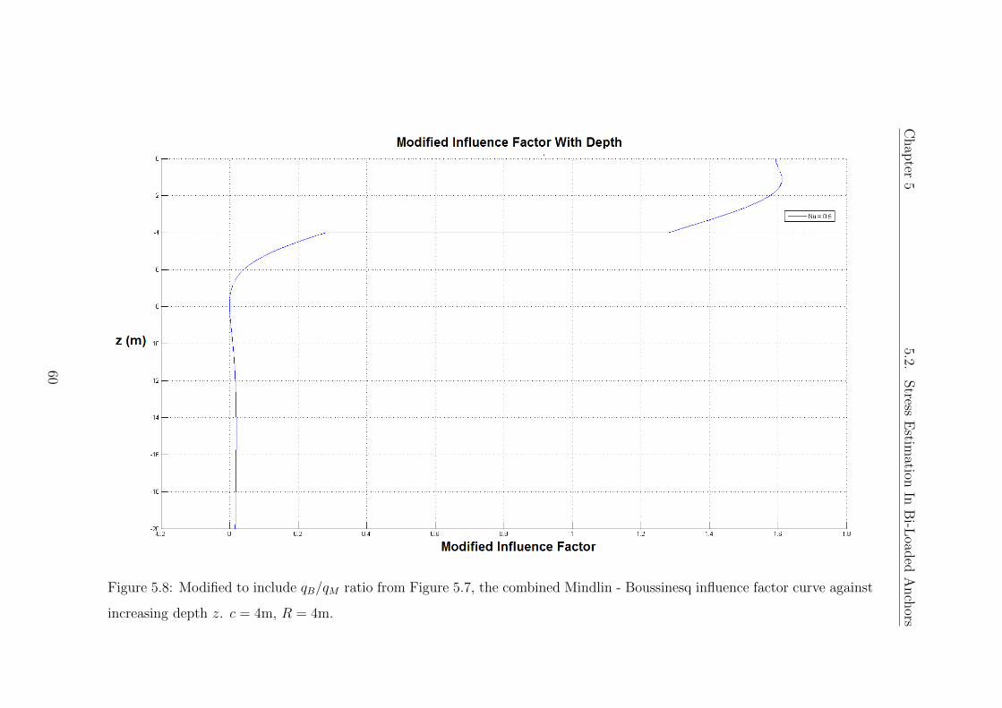
Using this equation for an array of z values gives Figure 5.7. Note that the peak
negative influence factor on Figure 5.6 occurs at a depth of 6.28m which does
not equal where the peak ratio is situated in Figure 5.7 which occurs at 7.9m.
This makes sense because again, Boussinesq’s equation is continually getting less
intense. Figure 5.8 is proof that implementing the ratio qB/qM = 1.593 obtained
from Figure 5.7 into the equation below eliminates all tensile stresses in the system.
I = IM + (qBqM
)IB
where,
IM is the Mindlin influence factor (σM/qM)
IB is the Boussinesq influence factor (σB/qB)
58

Chap
ter5
5.2.Stress
Estim
ationIn
Bi-L
oaded
Anch
ors
Figure 5.7: Ratio of loads required to nullify tensile stresses at depth z. c = 4m, R = 4m.
59
Chap
ter5
5.2.Stress
Estim
ationIn
Bi-L
oaded
Anch
ors
Figure 5.8: Modified to include qB/qM ratio from Figure 5.7, the combined Mindlin - Boussinesq influence factor curve against
increasing depth z. c = 4m, R = 4m.
60

Chap
ter5
5.2.Stress
Estim
ationIn
Bi-L
oaded
Anch
ors
Figure 5.9: Stress with depth, no surface load c = 7m, R = 2m, q = 200kPa
and γ = 18kN/m3.
61

Chap
ter5
5.2.Stress
Estim
ationIn
Bi-L
oaded
Anch
ors
Figure 5.10: Stress with depth, no surface load c = 7m, R = 2m, q = 300kPa
and γ = 18kN/m3.
62

Chapter 5 5.2. Stress Estimation In Bi-Loaded Anchors
Discussion of Figures 5.9 and 5.10
Figures 5.9 and 5.10 show the stress against depth when instead of a surface load,
the uplift force of the anchor is mitigated purely by the weight of the soil, γ
(kN/m3). The difference that can be observed between Figure 5.9 and Figure 5.10
is a demonstration of the ability and ease of which a parametric study can be
performed with these solutions. Figure 5.9 would indicate that the weight of the
soil is enough to ensure the anchor system is entirely in compression and therefore
would not fail, whereas figure 5.10 illustrates that increasing the Mindlin load from
200kPa to 300kPa and not changing any of the other variables would induce tensile
stresses and therefore possible soil failure for this particular case.
Summary
Similarly to the Mindlin based influence chart developed earlier, the figures up
until this point require numerical inputs for some parameters which limits their
practical value. Specific values of c, R and additionally in the second case, q
and γ must be chosen before the graphs can be generated. Although unlike the
Newmark styled influence chart from earlier, the figures created represent a visual
and insightful demonstration of how stress weakens with depth as well as the
entanglement of Boussinesq’s and Mindlin’s solutions and the overall influences
that certain parameters have within them.
5.2.4 Forming a Single Design Chart
As the value of qB/qM required to nullify tensile stresses depends entirely on R/c
(if both subsurface and surface loads have the same radius R, ie. RB = RM = R)
a table of values could be formulated giving the maximum ratio of qB/qM for each
R/c and from that, a graph. Given the complexity of Eq. 5.2, it is not possible
to directly equate qB/qM to R/c so another method must be used. This would
63

Chapter 5 5.2. Stress Estimation In Bi-Loaded Anchors
be a very time consuming task to do manually but the computational power of
MATLAB supplies a timely alternative. A major simplification in such a case
would be that RB = RM which, from a practical point of a view is not an overly
demanding requirement. Furthermore, optimization of radii against surface and
sub-surface loadings is possible with subsequent analysis.
Taking a look at Eq. 4.12 it can be seen that on the left hand side of the equation
we have units of pressure denoted by σz and on the right hand side of the equation
exterior to the main set of parentheses we also have a pressure given by q. Therefore
the final unit obtained through solving for the terms inside the parentheses must
be dimensionless. This allows that R, c and z to all be divided by c resulting in an
identical dimensionless answer. Doing so allows the performance of computations
with a unified variable R/c which is what is needed to determine maximum values
of qB/qM . This approach was undertaken in the MATLAB code, giving Figure
5.11.
64

Chap
ter5
5.2.Stress
Estim
ationIn
Bi-L
oaded
Anch
ors
Figure 5.11: Design chart providing the required ratio of qB/qM for each value of R/c.
65

Chapter 5 5.2. Stress Estimation In Bi-Loaded Anchors
Figure 5.11 represents a design chart which, assuming that the radius of Boussi-
nesq’s load is equal to that of the Mindlin’s load gives the required loading ratio on
the surface against the subsurface to nullify all tensile stresses within the system.
It was ensured that for each case, qB/qM achieved a maximum prior to reaching
the limiting value of z = 20m used in the MATLAB script. It is also important
to note that the chart does not take into account soil weight and thus it can be
deemed as conservative.
5.2.5 Conclusion and Limitations
A single design chart (Figure 5.11) was reached, however it makes the assumption
that RB = RM , which could be overcome by some further work on the solutions.
The set back that was encountered of not fully taking into account the variation of
stress intensity with depth was a great demonstration of the insight in which the
closed form solution can give. The closed form nature means that the plots are
exact and the graphical nature of the investigation allows for a quick visual inspec-
tion which is a useful educational tool. This section has also been an exhibition
into the flexibility of the closed form solution and the ease at which modifications
can be made.
Sabatini, Pass & Bachus (1999, pp. 68) state that when compression anchors (bi-
loaded anchors) are to be used for permanent application, pre-design test programs
may be required to assure satisfactory performance unless verification can be ob-
tained from prior experience or research results. It would seem that the results
(or similar) obtained from this thesis may be applicable to the aforementioned
pre-design stage to suggest plausibility as it should give a conservative estimate.
Although, it is likely that the results obtained here would need follow up work to
make them more applicable for practical use.
66

Chapter 5 5.2. Stress Estimation In Bi-Loaded Anchors
It is important to stress however that although the figures in this section are
focused on a practical topic, the anchor system analysed here is heavily simplified
and thus the results gathered here are not entirely realistic. In addition to the
aforementioned isotropic, homogeneous, elastic conditions of the soil media the
model assumes that the anchor is flexible and that the loads on the anchor are
uniformly distributed. It also neglects anchor thickness and for the bi-loaded case
does not take into account soil weight. Anchors in practice are almost always
angled, usually between 15 and 30 degrees (Sabatini, Pass & Bachus 1999, pp.70).
The anchor in this problem and its associated mathematics are applicable only for
an orientation normal to a horizontal surface. However an angled analysis would be
possible by amalgamating multiple equations from Mindlin’s solution for stresses
in different directions.
Overall both benefits and limitations of the closed form solution can be readily
seen throughout this section and a valid design chart was produced. Of further
note the answer from the example performed in Section 5.2 was verified as correct
using the MATLAB code. MATLAB code used for the creation of Figures 5.4 -
5.11 can be found in Appendix C.
67

Chapter 6
Conclusions and Further Work
6.1 Conclusions
Three related geotechnical, closed form solutions were chosen and researched. This
research showed the applications for which they can be used; mainly, tunnelling,
piling and anchoring. This research also gave an indication on the sorts of processes
in which the solutions may be subjected to and just what could be achieved.
Mindlin’s solution was successfully integrated for the vertical stress produced under
the center of a circular sub-surface loading. This solution was used to obtain charts
and plots that were compared and analysed. The first of which was a Newmark
styled Mindlin based influence chart that was deemed not practically useful due
to the fact that one chart would have to be produced for each configuration of
variables. The next array of plots were based on an anchor system of which Figure
5.11 represents the final, and the most practical. It is capable of giving some
conservative estimates in compression anchor design.
Of the main objectives outlined in the project specification (listed in Appendix
68

Chapter 6 6.2. Further Work
A), only the final and supplementary objective which was to compare the closed
form solutions with their numerical alternatives was not undertaken due to time
constraints.
On a whole the category of closed form solutions in geotechnical engineering was
reviewed throughout this project; their prominent benefits were that of insight and
flexibility and their main limitation, their simplifying assumptions.
6.2 Further Work
The mathematics for the anchor system that was investigated in Chapter 5 could
be modified as to be more realistic. Most especially re-orientating the anchor at
an angle and reducing a number of other unrealistic traits mentioned in Section
5.2.5.
In Section 5.2.3 an anchor system with no surface loading is examined and a small
parametric study is performed but no singular design chart was developed that
would show the depth required for an anchor to be placed so that purely the
weight of the soil would nullify tensile stresses. Interest in to the prospect of a
singular design chart for this case could be further investigated.
The reason for an I > 1 which is seen in Figure 5.4 is currently unknown. One
possible reason for the anomaly is that it is a created as a result of the circular
integration. If the same chart was generated for say, a rectangular integration the
reason could be explained.
Comparisons with numerical solutions were not performed due to time limitations
but would be a valuable source of information in certifying the overall value of
closed form solutions in this area, and evaluate the levels of error caused by sim-
plifying assumptions involved.
69

Chapter 6 6.2. Further Work
Kelvin’s solution was chosen as one to be investigated in this project, but no results
or data was obtained that was centred around it. One possible area of exploration
would be the application of Kelvin’s solution in deep tunnelling, where the effects
of the surface could be deemed negligible.
70
References
Altun, S., Karakan, E., and Tuna, S. C. (2013). Load displacement relationship
for a rigid circular foundation anchored by Mindlin soltuions. Scientia Iranica,
20(3):397–405.
Basile, F. (2002). Integrated form of singluar Mindlin’s solution. In Proc. 10th
ACME Conference, pages 191–194.
Bower, A. F. (2008). Analytical techniques and solutions for linear elastic solids.
http://solidmechanics.org/text/Chapter5_1/Chapter5_1.htm. Accessed
14 October 2014.
Butterfield, R. and Banerjee, P. (1971). The elastic analysis of compressible piles
and pile groups. Geotechnique, 21(1):43–60.
Chow, L. (1994). The prediction of surface settlements due to tunnelling in soft
ground. PhD thesis, Brasenose College, University of Oxford.
Das, B. M. and Sobhan, K. (2010). Principles of Geotechnical Engineering, SI.
Cengage Learning, Stamford, USA, 8th edition.
Dominguez, B. (1966). Stress and displacements in semi-infinite media. Master’s
thesis, Universidad Nacional de Bueonos Aires.
Douglas, D. J. and Davis, E. H. (1964). The movement of buried footings due to
moment and horizontal load and the movement of anchor plates. Geotechnique,
14(2):115–132.
71

Chapter 6 References
Dwight, H. B. (1957). Tables of integrals and other mathematical data. The Macmil-
lan Company, New York, 3rd edition.
Geddes, J. D. (1966). Stresses in foundation soils due to vertical subsurface loading.
Geotechnique, 16(3).
Geddes, J. D. (1969). Boussinesq-based approximations to the vertical stresses
caused by pile-type subsurface loadings. Geotechnique, 19(4):509–514.
Mindlin, R. (1936). Force at a point in the interior of a semi-infinite solid. Physics,
7(5):195–202.
Neumann, E. (2004). Numerical vs. analytical solutions. http://www.
myphysicslab.com/numerical_vs_analytic.html. Accessed 7 May 2014.
Perloff, W. H. and Baron, W. (1976). Soil Mechanics Principles and Applications.
John Wiley Sons.
Poulos, H. and Davis, E. (1974). Elastic Solutions for Soil and Rock Mechanics.
Centre for Geotechnical Research, University of Sydney.
Powrie, W. (2001). Soil Mechanics Concepts Applications. Spon Press, 2nd edition.
Rahman, M. and Newaz, G. (2000). Boussinesq type solution for transversely
isotropic half-space coated with a thin film. International Journal of Engineering
Science, 38(7):807–822.
Sabatini, P. J., Pass, D. G., and Bachus, R. C. (1999). Geotechnical Engineering
Circular No.4 - Ground Anchors and Anchored Systems. GeoSyntec Consultants,
1100 Lake Hearn Drive, Atlanta, Georgia.
Selvadurai, A. P. S. (1979). The displacement of a rigid circular foundation an-
chored to an isotropic elastic half-space. Geotechnique, 29(2):195–202.
Selvadurai, A. P. S. (2001). Mindlin’s problem for a halfspace with a bonded
flexural surface constraint. Mechanics Research Communications, 28(2):157–
164.
72

Chapter 6 References
Sun, H. S., Lei, G. H., Ng, C. W. W., and Zheng, Q. (2013). Displacements under
linearly distributed pressures by extended Mindlins equations. Computers and
Geotechnics, 50:143–149.
Tian-quan, Y. (1981). Pile analysis by simple integral equation methods. Applied
Mathematics and Mechanics, 2(3).
Timoshenko, S. and Goodier, J. (1951). Theory of Elasticity. McGraw-Hill Book
Company.
Vaziri, H., Simpson, B., Pappin, J. W., and Simpson, L. (1982). Integrated forms
of Mindlin’s equations. Geotechnique, 32(3):275–278.
Zhang, J. F., Chen, J. J., Wang, J. H., and Zhu, Y. F. (2013). Prediction of
tunnel displacement induced by adjacent excavation in soft soil. Tunnelling and
Underground Space Technology, 36:24–33.
73

Appendix A
Project Specification
74


Appendix B
General
76

Figure B.1: Mindlin based influence chart for test 1 performed in section 5.1
77

Figure B.2: Mindlin based influence chart for test 2 performed in section 5.1
78

Appendix C
MATLAB Code
79

function Inffactor = IntegMindlin_F(v,z,c,R)
%Calculating Terms of Equation 4.12 Individually
m = 3*(3-4*v)*z*(z+c).^2 - 3*c*(z+c)*(5*z-c); %Numerator for terms 7,8
tn = (1-2*v)*(z-c); %Numerator for terms 1-4
t1 = tn./[(R.^2+(z-c)^2).^0.5]; %Term 1
t2 = tn./[((z-c)^2).^0.5]; %Term 2
t3 = tn./[(R.^2+(z+c)^2).^0.5]; %Term 3
t4 = tn./[((z+c)^2).^0.5]; %Term 4
t5 = ((z-c)^3)./[(R.^2+(z-c)^2).^1.5]; %Term 5
t6 = ((z-c)^3)./[((z-c)^2).^1.5]; %Term 6
t7 = m./[3*(R.^2+(z+c)^2).^1.5]; %Term 7
t8 = m./[3*((z+c)^2).^1.5]; %Term 8
t9 = (6*c*z*(z+c)^3)./(R.^2+(z+c)^2).^2.5; %Term 9
t10 = (6*c*z*(z+c)^3)./((z+c)^2).^2.5; %Term 10
Inffactor = -(1./(4-4*v)).*(t1 - t2 - t3 + t4 + t5 - t6 + t7 - t8 + t9
- t10);
80

%ENG4111/4112 Research Project
%Name: Tim Eaton
%File: MindlinPlot_F.m
%For plotting Mindlin-Boussinesq Influence Factor Curves
%Last modified 14th September, 2014
clear all
close all
clc
z = 4; %Depth to point of interest (metres)
c = 3.99999; %Depth to Mindlin loading (metres)
R = 0:0.1:20; %Radius of circular distributed load (metres)
x = R/z;
for v = 0:0.1:0.5; %Poisson’s Ratio
y = IntegMindlin_F(v,z,c,R);
%Plotting
hold all
grid on
plot(x,y)
axis([0 5 0.5 1.05])
xlabel(’R/z’)
ylabel(’Influence Factor’)
title(’Mindlin - Boussinesq Influence Factor Curves z=c’);
end
%Calculating and plotting Boussinesq’s Equation
B = 1-(z.^3)./[(R.^2+z.^2).^(3/2)];
plot(x,B,’LineWidth’,2)
legend(’Nu = 0’,’Nu = 0.1’,’Nu = 0.2’,’Nu = 0.3’,’Nu = 0.4’,’Nu = 0.5’
,’Boussinesq’)
81

%ENG4111/4112 Research Project
%Name: Tim Eaton
%File: MindlinBoussinesqStresswithDepth.m
%For observing Mindlin - Boussinesq stress behaviour against depth
%Last modified 14th September, 2014
clear all
close all
clc
z = 0:0.001:20; %Depth to point of interest (metres)
c = 4.00001; %Depth to Mindlin loading (metres)
R = 1; %Radius of circular distributed load (metres)
for v = 0:0.1:0.5; %Poisson’s Ratio
x = IntegMindlin_F(v,z,c,R);
hold all
grid on
plot(x,-z)
ylabel(’z (m)’)
xlabel(’Influence Factor’)
title(’Mindlin - Boussinesq Influence Factor with Depth’);
end
%Calculating and plotting Boussinesq’s Equation
B = 1-(z.^3)./(R.^2+z.^2).^(3/2);
plot(B,-z,’LineWidth’,2)
legend(’Nu = 0’,’Nu = 0.1’,’Nu = 0.2’,’Nu = 0.3’,’Nu = 0.4’
,’Nu = 0.5’,’Boussinesq’)
82

%ENG4111/4112 Research Project
%Name: Tim Eaton
%File: CombinedPlot.m
%For observing Mindlin - Boussinesq COMBINED stress behaviour against depth
%Last modified 14th September, 2014
clear all
close all
clc
z = 0:0.001:20; %Depth to point of interest (metres)
c = 3.99999; %Depth to Mindlin loading (metres)
R = 4; %Radius of circular distributed load (metres)
%Calculating Boussinesq’s Equation
%1.233 obtained from script file MindlinPlot_F.m
B = 1-(z.^3)./((1.233*R)^2+z.^2).^(3/2);
for v = 0.5; %Poisson’s Ratio
x = IntegMindlin_F(v,z,c,R) + B;
hold all
grid on
plot(x,-z)
ylabel(’z (m)’)
xlabel(’Influence Factor’)
title(’Combined Mindlin - Boussinesq Influence Factor with Depth’);
legend(’Nu = 0.5’)
end
83
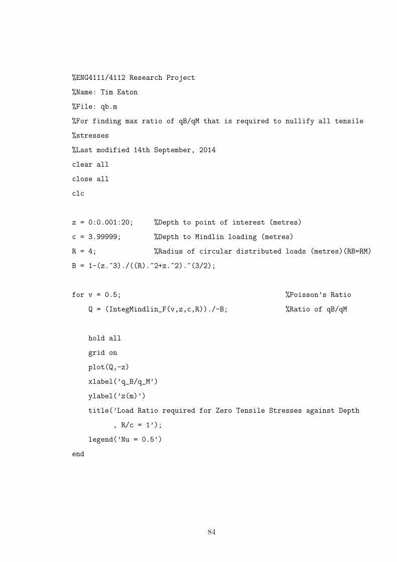
%ENG4111/4112 Research Project
%Name: Tim Eaton
%File: qb.m
%For finding max ratio of qB/qM that is required to nullify all tensile
%stresses
%Last modified 14th September, 2014
clear all
close all
clc
z = 0:0.001:20; %Depth to point of interest (metres)
c = 3.99999; %Depth to Mindlin loading (metres)
R = 4; %Radius of circular distributed loads (metres)(RB=RM)
B = 1-(z.^3)./((R).^2+z.^2).^(3/2);
for v = 0.5; %Poisson’s Ratio
Q = (IntegMindlin_F(v,z,c,R))./-B; %Ratio of qB/qM
hold all
grid on
plot(Q,-z)
xlabel(’q_B/q_M’)
ylabel(’z(m)’)
title(’Load Ratio required for Zero Tensile Stresses against Depth
, R/c = 1’);
legend(’Nu = 0.5’)
end
84

%ENG4111/4112 Research Project
%Name: Tim Eaton
%File: ModifiedIF.m
%For checking ratio obtained from script qb.m
%Last modified 14th September, 2014
clear all
close all
clc
z = 0:0.001:20; %Depth to point of interest (metres)
c = 3.99999; %Depth to Mindlin loading (metres)
R = 4; %Radius of circular distributed load (metres)
Q = 1.593; %qB/qM ratio obtained from script qb.m plot
%Calculating Boussinesq’s Equation
B = 1-(z.^3)./((R)^2+z.^2).^(3/2);
for v = 0.5; %Poisson’s Ratio
y = IntegMindlin_F(v,z,c,R) + Q*B;
hold all
grid on
plot(y,-z)
xlabel(’Modified Influence Factor’)
ylabel(’z(m)’)
title(’Modified Influence Factor with Depth’);
legend(’Nu = 0.5’)
end
85

%ENG4111/4112 Research Project
%Name: Tim Eaton
%File: nosurcharge.m
%For seeing at what depth Mindlin stresses are canceled out by self weight
%of soil
%Last modified 18th September, 2014
clear all
close all
clc
z = 0:0.001:20; %Depth to point of interest (metres)
c = 7.00001; %Depth to Mindlin loading (metres)
R = 2; %Radius of circular distributed load (metres)
q = 300; %Mindlin load kPa
gamma = 18; %Unit weight of the soil kN/m^3
G = gamma.*z; %Stress due to soil weight kPa
for v = 0:0.1:0.5; %Poisson’s Ratio
x = IntegMindlin_F(v,z,c,R).*q + G;
hold all
grid on
plot(x,-z)
ylabel(’z (m)’)
xlabel(’Stress (kPa)’)
title(’Mindlin vs soil weight with Depth’);
legend(’Nu = 0’,’Nu = 0.1’,’Nu = 0.2’,’Nu = 0.3’,’Nu = 0.4’
,’Nu = 0.5’)
end
86

%ENG4111/4112 Research Project
%Name: Tim Eaton
%File: qratio_max_plot.m
%For finding max values of qB/qM that is required to nullify all tensile
%stresses for each value of R/c
%Last modified 12th October, 2014
clear all
close all
clc
Z = 0:0.001:20; %Depth to point of interest (metres)
C = 1.99999; %Depth to Mindlin loading (metres)
z = Z./C; %dimensionless transformation
c = 1; %dimensionless transformation
%r = Radius of circular distribute loads (metres)(RB=RM)
%v = Poisson’s ratio
%Q = Ratio of qB/qM
%%%%%%CASE 1%%%%%%
i=0;
v = 0.5;
for r = 0.00001:0.1:10.00001;
R = r./C;
i = i+1;
A(i) = r./C;
B = 1-(Z.^3)./((r).^2+Z.^2).^(3/2);
Q = (IntegMindlin_F(v,z,c,R))./-B;
qmax(i) = max(Q);
hold all
87
grid on
plot(A,qmax)
axis([0 5 1 6])
ylabel(’Ratio of q_B to q_M’)
xlabel(’R/c’)
title(’Required ratio q_B/q_M to nullify all Tensile Stresses’)
end
%%%%%%CASE 2%%%%%%
v=0.4;
for r = 0.00001:0.1:10.00001;
R = r./C;
i = i+1;
A4(i) = r./C;
B = 1-(Z.^3)./((r).^2+Z.^2).^(3/2);
Q = (IntegMindlin_F(v,z,c,R))./-B;
qmax4(i) = max(Q);
plot(A4,qmax4)
end
%%%%%%CASE 3%%%%%%
v=0.3;
for r = 0.00001:0.1:10.00001;
R = r./C;
i = i+1;
A3(i) = r./C;
B = 1-(Z.^3)./((r).^2+Z.^2).^(3/2);
Q = (IntegMindlin_F(v,z,c,R))./-B;
qmax3(i) = max(Q);
88

plot(A3,qmax3)
end
%%%%%%CASE 4%%%%%%
v=0.2;
for r = 0.00001:0.1:10.00001;
R = r./C;
i = i+1;
A2(i) = r./C;
B = 1-(Z.^3)./((r).^2+Z.^2).^(3/2);
Q = (IntegMindlin_F(v,z,c,R))./-B;
qmax2(i) = max(Q);
plot(A2,qmax2)
end
%%%%%%CASE 5%%%%%%
v=0.1;
for r = 0.00001:0.1:10.00001;
R = r./C;
i = i+1;
A1(i) = r./C;
B = 1-(Z.^3)./((r).^2+Z.^2).^(3/2);
Q = (IntegMindlin_F(v,z,c,R))./-B;
qmax1(i) = max(Q);
plot(A1,qmax1)
legend(’v = 0.1’,’v = 0.2’,’v = 0.3’,’v = 0.4’,’v = 0.5’)
end
89

90