Exploring the Bullwhip Effect and Inventory Stability in a ...cdn.intechopen.com/...bullwhip_effect_and_inventory_stability_in_a...International Journal of Engineering Business Management

International Journal of Engineering Business Management Special Issue on Innovations in Fashion Industry

Exploring the Bullwhip Effect and Inventory Stability in a Seasonal Supply Chain Regular Paper

Francesco Costantino1, Giulio Di Gravio1,*, Ahmed Shaban1,2 and Massimo Tronci1 1 Department of Mechanical and Aerospace Engineering, University of Rome “La Sapienza”, Rome, Italy 2 Department of Industrial Engineering, Fayoum University, Fayoum, Egypt * Corresponding author E-mail: [email protected]

Received 1 June 2013; Accepted 15 July 2013 DOI: 10.5772/56833 © 2013 Costantino et al.; licensee InTech. This is an open access article distributed under the terms of the Creative Commons Attribution License (http://creativecommons.org/licenses/by/3.0), which permits unrestricted use, distribution, and reproduction in any medium, provided the original work is properly cited.

Abstract The bullwhip effect is defined as the distortion of demand information as one moves upstream in the supply chain, causing severe inefficiencies in the whole supply chain. Although extensive research has been conducted to study the causes of the bullwhip effect and seek mitigation solutions with respect to several demand processes, less attention has been devoted to the impact of seasonal demand in multi‐echelon supply chains. This paper considers a simulation approach to study the effect of demand seasonality on the bullwhip effect and inventory stability in a four‐echelon supply chain that adopts a base stock ordering policy with a moving average method. The results show that high seasonality levels reduce the bullwhip effect ratio, inventory variance ratio, and average fill rate to a great extent; especially when the demand noise is low. In contrast, all the performance measures become less sensitive to the seasonality level when the noise is high. This performance indicates that using the ratios to measure seasonal supply chain dynamics is misleading, and that it is better to directly use the variance (without dividing by the demand variance) as the estimates for the bullwhip

effect and inventory performance. The results also show that the supply chain performances are highly sensitive to forecasting and safety stock parameters, regardless of the seasonality level. Furthermore, the impact of information sharing quantification shows that all the performance measures are improved regardless of demand seasonality. With information sharing, the bullwhip effect and inventory variance ratios are consistent with average fill rate results. Keywords Supply Chain, Information Sharing, Bullwhip Effect, Seasonal Demand, Inventory Variance Ratio, Order Variance, Inventory Variance, Order‐Up‐To, Fill Rate, Simulation

1. Introduction A supply chain is defined as a system of suppliers, manufacturers, distributors, retailers, and customers where raw materials, finances and information flows connect participants in both directions. The main

Francesco Costantino, Giulio Di Gravio, Ahmed Shaban and Massimo Tronci: Exploring the Bullwhip Effect and Inventory Stability in a Seasonal Supply Chain

1www.intechopen.com

ARTICLE

www.intechopen.com Int. j. eng. bus. manag., 2013, Vol. 5, Special Issue Innovations in Fashion Industry, 23:2013

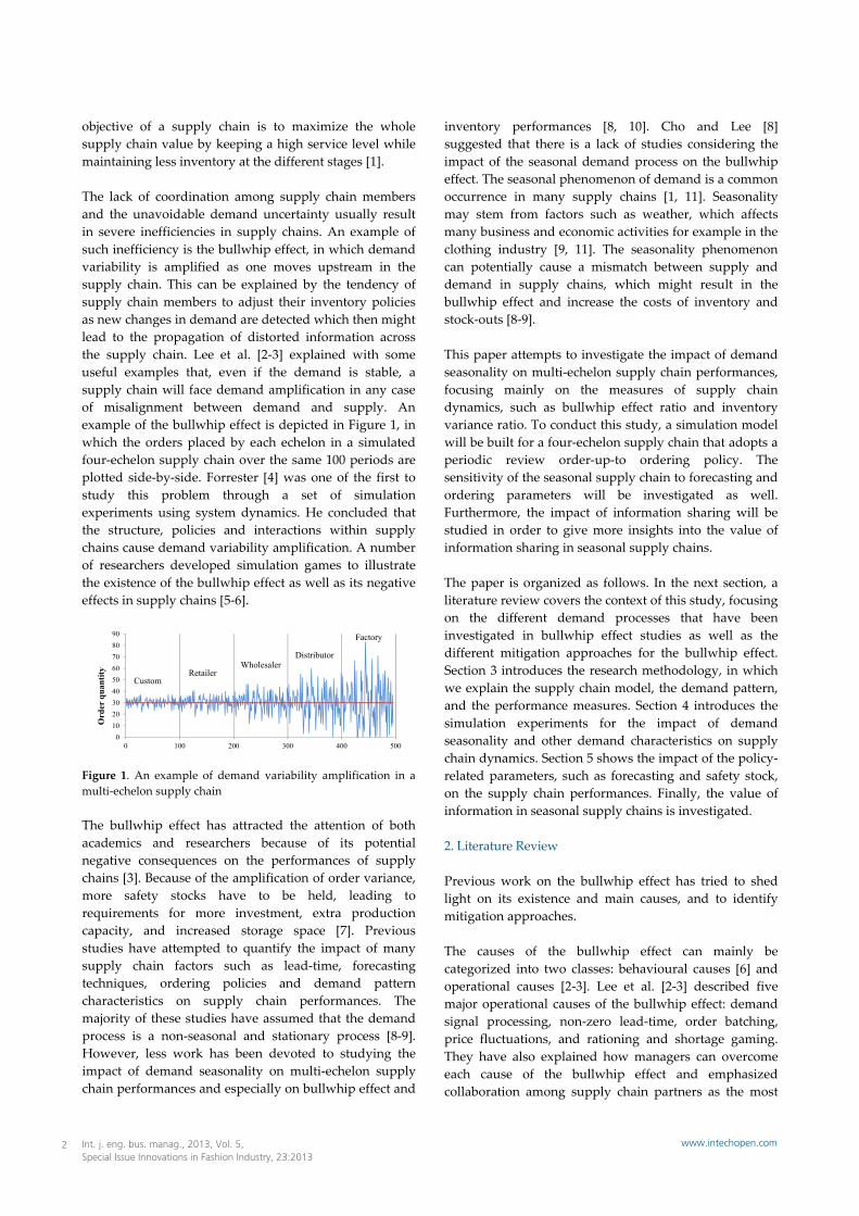
objective of a supply chain is to maximize the whole supply chain value by keeping a high service level while maintaining less inventory at the different stages [1]. The lack of coordination among supply chain members and the unavoidable demand uncertainty usually result in severe inefficiencies in supply chains. An example of such inefficiency is the bullwhip effect, in which demand variability is amplified as one moves upstream in the supply chain. This can be explained by the tendency of supply chain members to adjust their inventory policies as new changes in demand are detected which then might lead to the propagation of distorted information across the supply chain. Lee et al. [2‐3] explained with some useful examples that, even if the demand is stable, a supply chain will face demand amplification in any case of misalignment between demand and supply. An example of the bullwhip effect is depicted in Figure 1, in which the orders placed by each echelon in a simulated four‐echelon supply chain over the same 100 periods are plotted side‐by‐side. Forrester [4] was one of the first to study this problem through a set of simulation experiments using system dynamics. He concluded that the structure, policies and interactions within supply chains cause demand variability amplification. A number of researchers developed simulation games to illustrate the existence of the bullwhip effect as well as its negative effects in supply chains [5‐6].

Figure 1. An example of demand variability amplification in a multi‐echelon supply chain The bullwhip effect has attracted the attention of both academics and researchers because of its potential negative consequences on the performances of supply chains [3]. Because of the amplification of order variance, more safety stocks have to be held, leading to requirements for more investment, extra production capacity, and increased storage space [7]. Previous studies have attempted to quantify the impact of many supply chain factors such as lead‐time, forecasting techniques, ordering policies and demand pattern characteristics on supply chain performances. The majority of these studies have assumed that the demand process is a non‐seasonal and stationary process [8‐9]. However, less work has been devoted to studying the impact of demand seasonality on multi‐echelon supply chain performances and especially on bullwhip effect and

inventory performances [8, 10]. Cho and Lee [8] suggested that there is a lack of studies considering the impact of the seasonal demand process on the bullwhip effect. The seasonal phenomenon of demand is a common occurrence in many supply chains [1, 11]. Seasonality may stem from factors such as weather, which affects many business and economic activities for example in the clothing industry [9, 11]. The seasonality phenomenon can potentially cause a mismatch between supply and demand in supply chains, which might result in the bullwhip effect and increase the costs of inventory and stock‐outs [8‐9]. This paper attempts to investigate the impact of demand seasonality on multi‐echelon supply chain performances, focusing mainly on the measures of supply chain dynamics, such as bullwhip effect ratio and inventory variance ratio. To conduct this study, a simulation model will be built for a four‐echelon supply chain that adopts a periodic review order‐up‐to ordering policy. The sensitivity of the seasonal supply chain to forecasting and ordering parameters will be investigated as well. Furthermore, the impact of information sharing will be studied in order to give more insights into the value of information sharing in seasonal supply chains. The paper is organized as follows. In the next section, a literature review covers the context of this study, focusing on the different demand processes that have been investigated in bullwhip effect studies as well as the different mitigation approaches for the bullwhip effect. Section 3 introduces the research methodology, in which we explain the supply chain model, the demand pattern, and the performance measures. Section 4 introduces the simulation experiments for the impact of demand seasonality and other demand characteristics on supply chain dynamics. Section 5 shows the impact of the policy‐related parameters, such as forecasting and safety stock, on the supply chain performances. Finally, the value of information in seasonal supply chains is investigated. 2. Literature Review Previous work on the bullwhip effect has tried to shed light on its existence and main causes, and to identify mitigation approaches. The causes of the bullwhip effect can mainly be categorized into two classes: behavioural causes [6] and operational causes [2‐3]. Lee et al. [2‐3] described five major operational causes of the bullwhip effect: demand signal processing, non‐zero lead‐time, order batching, price fluctuations, and rationing and shortage gaming. They have also explained how managers can overcome each cause of the bullwhip effect and emphasized collaboration among supply chain partners as the most

0102030405060708090

0 100 200 300 400 500

Ord

er q

uant

ity

CustomRetailer

WholesalerDistributor

Factory

Int. j. eng. bus. manag., 2013, Vol. 5, Special Issue Innovations in Fashion Industry, 23:2013

2 www.intechopen.com

important solution. Subsequently, extensive research has been conducted to quantify the bullwhip effect while considering these causes based on four modelling approaches: statistical, control theoretic, simulation games, and simulation. The statistical approaches have been mainly used to derive closed‐form expressions for the bullwhip effect [3, 12‐15] and recently for net inventory variance [14, 16‐17] under specific supply chain settings. The control theoretic approaches have also been used as an equivalent alternative to the statistical approaches; in particular, this approach has been utilized to design ordering policies to smooth placed orders [18‐20]. Hosoda and Disney [17] pointed out that “the statistical approaches become unmanageable when net inventory variances are considered for measuring the inventory performance because the expressions for the covariance between the states of the system become very complex to derive”. Different simulation modelling approaches have also been used to study supply chain dynamics; some authors adopted system dynamics [21‐22] and others discrete‐event simulation [7, 23‐25]. In this paper, we adopt a simulation approach since we aim to study the impact of demand seasonality in a multi‐echelon supply chain, which is a complex system to solve with analytical models. We further estimate some measures (e.g., inventory variance) that cannot be easily obtained by analytical approaches. Several authors have focused on the impact of forecasting techniques, lead‐time and ordering policies on the bullwhip effect in order to give useful insights on the optimum operational practices under different settings and assumptions [3, 12‐15, 21‐22]. The majority of these studies have assumed that the demand process is a non‐seasonal and stationary process and have modelled it as an autoregressive moving average (ARMA) process type of the first order. Of particular interest to us, Chen et al. [12] used an auto‐regressive AR(1) demand process for a two‐echelon serial supply chain and derived analytically a lower bound of the bullwhip effect, when the retailer employs the order‐up‐to with the moving average (MA) method to forecast lead‐time demand. Chen et al. [13] and Xu et al. [26] obtained similar results when the exponential smoothing technique is employed for forecasting. Chen et al. [13] indicated also that if a smoothing parameter in exponential smoothing is set in order to achieve equal forecasting accuracy for both exponential smoothing and moving average methods, then exponential smoothing gives larger order variance. Alwan et al. [27] studied the bullwhip effect under a base‐stock policy applying the Mean Squared Error optimal forecasting method to an AR(1) and investigated further the stochastic nature of the ordering process for an incoming ARMA(1,1) using the same inventory policy and forecasting technique. Duc et al. [28] quantified the bullwhip effect for a two‐stage supply chain in which the

demand process followed ARMA(1, 1) with a base‐stock policy with the MMSE method used at the retailer. They analytically investigated the effects of the autoregressive coefficient, the moving average coefficient, and the lead‐time on the bullwhip effect. Many other studies have adopted the normality assumption of the external demand to study the bullwhip effect [7, 19, 23‐25]. Recently, some authors have adopted artificial intelligence techniques such as fuzzy logic in order to model supply chain operations and external demand [29]. Limited research has been conducted to explore the effect of demand seasonality on the demand variability amplification in multi‐echelon supply chains [8]. Cho and Lee [8] adopted an analytical approach to quantify the bullwhip effect in a two‐echelon supply chain in which the external demand is a SARMA (1, 0) X (0,1)s scheme, a seasonal autoregressive‐moving average process, and the retailer places his orders based on a base stock policy. They further extended their work by studying the value of information sharing in a two‐echelon supply chain by evaluating the bullwhip effect under three information‐sharing scenarios [9]. Lau et al. [30] investigated via simulation the effects of information sharing and early order commitment on the performance of four inventory policies used by retailers facing seasonal demand in a supply chain of one capacitated supplier and four retailers. Bayraktar et al. [10] analysed the impact of exponential smoothing forecasts on the bullwhip effect for electronic supply chain management (E‐SCM) applications and they considered the external demand to have a seasonal component. They concluded that, although high seasonality reduces the forecast accuracy, it has a positive influence on the reduction of the bullwhip effect. Different mitigation approaches have been suggested to handle the bullwhip effect in supply chains. Most importantly, collaboration has been proven to have a significant impact on supply chain performances and the bullwhip effect [31‐33]. Several authors have examined the impact of collaboration initiatives such as vendor‐managed inventory (VMI) on the bullwhip effect [3, 34‐36]. Many other studies have examined the impact of sharing customer demand information [7, 9, 21, 30, 37]. Recently, innovative information‐sharing polices requiring less implementation effort have been proposed by Costantino et al. [24] to improve supply chain dynamics, and other authors have also introduced a modelling formalism for the synchronized supply chain that needs full visibility of supply chain information [38]. In this research, we investigate the impact of information sharing in seasonal supply chains. The literature analysis reveals that relatively little work has been devoted to exploring the impact of seasonal demand


3www.intechopen.com

on the bullwhip effect and inventory performances, especially in multi‐echelon supply chains. This study is an attempt to fill this gap by studying the effect of seasonal demand and its interaction with other parameters in a multi‐echelon supply chain through a simulation study. In particular, the impact of other bullwhip causes such as the forecasting and ordering policy parameters will be investigated jointly with the seasonality level. Finally, information sharing as a mitigation approach will be evaluated in a seasonal supply chain. 3. Research Methodology

3.1 Supply Chain Model

In this research, we model a multi‐echelon supply chain that consists of a customer, a retailer, a wholesaler, a distributor, and a factory to conduct various investigations (see Figure 2). This is a well‐known supply chain model, known as the Beer Game structure, and has been utilized in many previous bullwhip effect investigations [7, 23‐25, 38]. It is assumed that all echelons have unlimited stocking capacity, both the supplier and the factory have unlimited capacity, and the ordering and delivery lead‐times are deterministic and fixed across the supply chain, with ordering lead‐time = 1 and delivery lead‐time = 2.

Figure 2. A multi‐echelon supply chain We assume that each echelon in the supply chain employs the order‐up‐to ordering policy (base stock policy). This ordering policy has been widely considered in the literature of supply chain dynamics because of its popularity in practice [39]. In this policy, at the end of each review period ( R ), an order i

tO is placed whenever the inventory position i

tIP is lower than a specific target level i

tS (see equation (1)). The inventory position represents the difference between 1

itS and the incoming

order itIO , as shown in equation (2). The review period is

considered to be equal to one (i.e., 1R ).

{( ),0}i i it t tO Max S IP (1)

1i i i

t t tIP S IO (2)

The target inventory position itS (order up to level) is

calculated based on the expected demand over the total lead‐time (ordering and delivery lead‐times) plus the safety stock component ( i

tSS ). This can be represented as shown in equation (3).

ˆi i it t tS LD SS (3)

The moving average forecasting technique is considered to calculate the expected demand ( ˆ i

tD ) because of its popularity both in research and in practice [12‐13, 39]. The future demand is calculated based on the last consecutive in incoming orders/demand, as shown in equation (4), where in is the averaging time.

11

1ˆin

i it t j

ji

D IOn

(4)

We have considered the safety stock component in equation (3) by extending the lead‐time by ik ; this approach is more practical and is common in the bullwhip effect literature [19, 25]. The target inventory position i

tS can be rewritten as in equation (5).

ˆ( )i it i tS L k D (5)

3.2 Demand Model

As the main objective of this paper is to quantify the bullwhip effect and inventory performance in a seasonal multi‐echelon supply chain, the external demand ( tD ) faced by the retailer is generated to have a seasonal component according to the formula in equation (6). This demand generator has been given by Zhao and Xie [40] and consists of constant demand (parameter, base ), trend component (parameter, slope ), seasonal components (sinusoidal function with parameters season and SeasonCycle ), and noise component (parameter, ). Accordingly, different demand patterns with different characteristics can be generated using the below formula. For all demand patterns across this paper, the trend component is neglected (i.e.,

0slope ) unless something else is mentioned. Furthermore, the demand parameters will be selected in a way that avoids generating negative values by selecting the base value to be high enough in comparison to season and .

22sin N 0,

tD base slope t

season tSeasonCycle

(6)

3.3 Performance Measures The objective of this study is to investigate the impact of seasonal demand characteristics in a multi‐echelon supply chain in terms of demand variability amplification and the corresponding inventory performance across the supply chain. To this end, three performance measures are considered: bullwhip effect ratio, inventory variance ratio, and average fill rate.



3.3.1 Bullwhip Effect Ratio

The bullwhip effect ratio has been widely used in the literature on supply chain dynamics [24, 38, 39]. The bullwhip effect ratio expresses the amplification of demand variability across the supply chain. In particular, Chen et al. [12] quantified the bullwhip effect ( iBWE )

analytically in terms of the variance of the orders ( 2iO )

placed by echelon i relative to the variance of the demand faced by the retailer, both divided by their respective means. Therefore, the bullwhip effect can be quantified according to the formula in equation (7).

2

2

//

i iO Oi

D D

BWE

(7)

3.3.2 Inventory Variance Ratio

The second measure is called inventory variance ratio, which was proposed by Disney and Towill [41] to measure the degree of inventory stability. This quantifies the fluctuations in net inventory ( 2

iNI ) relative to the

fluctuations in demand variability ( 2D ), as seen in

equation (8). It can also measure the amplification in inventory instability as we move up the supply chain [38]. An increased inventory variance ratio would result in higher holding and backlog costs, lower service level and increasing average inventory costs per period [39].

2

2iNI

iD

InvR

(8)

3.3.3 Average Fill Rate

The average fill rate is representative of customer service level, since it quantifies the percentage of items delivered immediately by echelon i to satisfy an incoming order [42]. Fill rate ( i

tFR ) is computed every time there is a positive incoming order (i.e., when 0i

tIO ), as shown in equation (9), where i

tSR stands for the shipment released by echelon i at t , 1

itB stands for the initial backlog at echelon i at t ,

and itIO is the incoming order to echelon i at time t . The

effective simulation time is equivalent to the summation of all periods with 0i

tIO ; hence, effT T . Its time series

constitutes the history of the delivery system effectiveness that will be used to calculate the average fill rate ( iAFR ).

11

1

100 0

0 0

i ii it tt tii

tti it t

SR B if SR BIOFR

if SR B

(9)

1effT i

tti

eff

SLAFR

T (10)

The average fill rate ( iAFR ) is computed only over the effective simulation time ( effT ), as indicated in equation

(10). This measure will be calculated for all echelons in the supply chain in order to find a relationship between bullwhip effect ratio, inventory variance ratio and average service level in the seasonal supply chain. 4. Simulation Experiments and Results A simulation model was developed considering the above multi‐echelon supply chain model using the SIMUL8 simulation package. The simulation model and the demand generator were then verified and validated through a large number tests. 4.1 The impact of demand characteristics The impact of demand seasonality was evaluated by quantifying the bullwhip effect ratio, inventory variance ratio and average fill rate under four seasonal levels, 0, 5, 10 and 15 units, keeping the slope equal to zero and the base demand fixed and equal to 100 units in all scenarios. The experiments were carried out under three different levels of the noise, 5 , 10 and 15 units, in order to understand the interaction effect between the seasonality and the noise on the supply chain performances. For all scenarios, the forecasting and safety stock parameters were considered as 10in and 1ik , respectively. To conduct the experiments, in each scenario the simulation model was run for 10 replications of 1200 periods each, considering the first 200 periods as a warm‐up period. 4.1.1 Bullwhip Effect Analysis The impact of seasonality on the bullwhip effect under different noise levels ( ) is summarized in Figure 3. The results show that the bullwhip effect is present in all cases and the demand variability seems to increase geometrically across the supply chain, from the retailer to the factory. This conclusion is similar to the findings of Chatfield et al. [7], Costantino et al. [24] and Dejonkheere et al. [19] regarding a normally distributed demand process. It can be further observed that increased seasonality level helps to reduce the bullwhip effect regardless of the noise level of the demand process. This happens because the higher seasonality cancels the amplification in the order variability, as confirmed by Bayraktar et al. [10] who studied the bullwhip effect in relation to a two‐echelon E‐Supply Chain with seasonal demand. It can also be observed that the higher noise level helps to reduce the impact of seasonality on the bullwhip effect at all echelons. When there is no seasonality ( 0season ), higher levels of noise result in lower bullwhip effect. However, when seasonality is present and high, larger noise levels leads to a higher bullwhip effect in comparison to lower noise levels. As can


5www.intechopen.com

be seen, the gap between the bullwhip effect ratios produced by each echelon under the different seasonality levels, across the supply chain, becomes very narrow when both the seasonality and the noise are high (Figure 3c).

Figure 3. The impact of seasonality on the bullwhip effect under different standard deviations In addition to the above analysis, we also investigated the impact of different seasonal cycles with different levels of seasonality on the bullwhip effect in the supply chain. The results are depicted in Figure 4 and show that as the seasonal cycle increases, the bullwhip effect decreases. This conclusion is the same under the two different levels of seasonality. However, the bullwhip effect ratio will be very high when the seasonality is high and the seasonal cycle is low.

Figure 4. The impact of seasonal cycle on the bullwhip effect under different seasonality levels

4.1.2 Inventory Performance Analysis The inventory performance is evaluated through two measures: inventory variance ratio and average fill rate. The results of the inventory variance ratio under the different combinations of the demand seasonality and noise levels are exhibited in Figure 5. It can be seen that the inventory variance ratio increases geometrically in the upstream direction for all combinations of seasonality and noise levels (Figure 5a‐c). The results further show that increased seasonality leads to increased inventory variance ratio to some extent at the downstream echelons, especially when the noise level is high. However, the inventory variance ratio tends to decrease at the upstream echelons with higher seasonality. This can be explained by the above results on the bullwhip effect with seasonality, as the bullwhip effect propagation across the supply chain tends to decrease when the seasonality level is higher. Again, similar to the bullwhip effect results, the gap between inventory variance ratios at each echelon under the different seasonality levels across the supply chain becomes very narrow when both the seasonality and the noise are high (Figure 5c).

Figure 5. The impact of seasonality level on the inventory variance ratio under different standard deviations

05

1015202530354045

Retailer Wholesaler Distributor Factory

Bullw

hip e

ffect

ratio

Supply chain echelon

(a) σ = 5

Season = 0 Season = 5Season = 10 Season = 15

0

10

20

30

40


Bullw

hip e

ffect

ratio


(b) σ = 10


0

5

10

15

20

25

30

35


Bullw

hip e

ffect

ratio


(c) σ = 15


0

10

20

30

40

50

60

7 28 52 100 7 28 52 100

Season=5 Season=15

Bullw

hip

effe

ct ra

tio

Season_Cycle


0102030405060708090


Inve

ntor

y va

rianc

e rat

io


(a) σ = 5


0102030405060708090


Inve

ntor

y var

ianc

e rat

io


(b) σ = 10


0102030405060708090


Inve

ntor

y va

rianc

e rat

io


(c) σ = 15




The impact of the seasonal cycle on the inventory variance ratio under different seasonality levels is depicted in Figure 6. The results reveal that the inventory variance ratio will be very high when the seasonal cycle is small and the seasonality level is high. It can also be argued that when the seasonality level is small, the inventory variance ratio will be less sensitive to the seasonal cycle. The lowest inventory variance ratio is realized when both the seasonality level and the seasonal cycle are very high (Figure 6).

Figure 6. The impact of seasonal cycle on the inventory variance ratio under different seasonality levels The average fill rate under the different combinations of seasonality and noise levels, at each echelon in the supply chain, is presented in Figure 7. It can be seen that the highest average fill rates are realized when both the seasonality and noise are low (Figure 7a). As the seasonality increases, the average fill rate decreases as we move upstream in the supply chain, regardless of the noise level, which means that the upstream echelons are prone to additional inventory costs due to the demand seasonality. This can be attributed to the failure of upstream echelons to account for demand seasonality as we move upstream in the supply chain. Furthermore, as expected, a higher noise level reduces the average fill rate, especially when the seasonality is high. The joint impact of the seasonality and the seasonal cycle is depicted in Figure 8. The results show that an acceptable average fill rate is realized across the supply chain when the seasonal cycle is high, whatever the seasonality level. For example, when the seasonal cycle is high ( 52SeasonCycle ), the average fill rate seems to be the same under both the seasonality levels. This can be attributed to the ability of each partner in the supply chain to meet the incoming orders when the seasonal cycle is long and the demand changes are lower to some extent. It can also be observed that high seasonality with low seasonal cycle leads to an unacceptable average fill rate. With lower seasonality, the supply chain is less sensitive to the seasonal cycle change, as can be inferred from the results in Figure 8.

Figure 7. The impact of seasonality level on the average fill rate under different standard deviations

Figure 8. The impact of the seasonal cycle on the average fill rate under different seasonality levels There is a paradox here: the results show that larger demand seasonality results in lower bullwhip effect and inventory variance ratios whilst the average fill rate is decreased, as explained above. It is common for the inventory variance to increase as the bullwhip effect increases, and thus the average fill rate decreases. Therefore, these results are misleading; this can be attributed to the characteristics of the performance measures used to quantify the bullwhip effect and inventory stability. Using the ratios ( iBWE and iInvR )

0

50

100

150

200

250

300

7 28 52 100 7 28 52 100

Season=5 Season=15

Inve

ntor

y va

rian

ce r

atio

Season_Cycle


95

96

97

98

99

100

101


Aver

age f

ill ra

te


(a) σ = 5


86889092949698

100102


Aver

age f

ill ra

te


(b) σ = 10


75

80

85

90

95

100

105


Aver

age f

ill ra

te


(c) σ = 15


0

20

40

60

80

100

120

7 28 52 100 7 28 52 100

Season=5 Season=15

Aver

age

fill r

ate

Season_Cycle



7www.intechopen.com

when the demand is seasonal and the seasonality level is high, the ratios tend to hide the content of information distortion in the supply chain, leading to misleading conclusions about the real dynamics in the chain. Therefore, it is better to quantify the bullwhip effect and inventory stability using the variance estimates without dividing by the demand variance. This is better clarified in Figure 9, in which we present again the results from Figures 3, 5 and 7 but in terms of the variance estimates along with the average fill rate, in order to show the consistency with these performance measures. The results in Figure 9 reveal that the order variance and inventory variance increase exponentially whilst the average fill rate decreases as both the seasonality and the noise increase. These results with variances seem more consistent in comparison to the above results that rely on the ratios.

Figure 9. The joint impact of seasonality and noise on the order variance, inventory variance and average fill rate 5. The impact of policy‐related parameters It has been recognized that forecasting and ordering policy are two main causes of the bullwhip effect [2‐3, 19]. Therefore, it is worth studying the impact of the safety stock parameter and the moving average parameter on seasonal supply chain performances. To conduct this analysis, we consider the following demand characteristics: 100base , 52SeasonCycle and 10 .

For each scenario, the simulation model was run for 10 replications of 1200 periods each, considering the first 200 periods as a warm‐up period. 5.1 The impact of the forecasting parameter We analysed the impact of the moving average parameter under two different levels of demand seasonality. The safety stock parameter was kept the same at 1ik for all scenarios. The results of the supply chain performances ( iBWE , iInvR and iAFR ) under the different scenarios of seasonality and moving average parameters are presented in Figure 10. The results reveal that using larger values of the moving average parameter decreases both the bullwhip effect and inventory variance ratios whilst improving the average fill rate. It can also be observed that the reduction in both bullwhip effect and inventory variance ratios will be greater when demand seasonality is high. This conclusion has already been explained above. Furthermore, it can be argued that using larger values of the moving average parameter makes the bullwhip effect less sensitive to the seasonality level.

Figure 10. The impact of the moving average parameter on the supply chain performances 5.2 The impact of the safety stock parameter We analysed the impact of the safety stock parameter on the supply chain performances under two different levels

010002000300040005000600070008000

Seas

on =

0

Seas

on =

5

Seas

on =

10

Seas

on =

15

Seas

on =

0

Seas

on =

5

Seas

on =

10

Seas

on =

15

Seas

on =

0

Seas

on =

5

Seas

on =

10

Seas

on =

15

Sigma = 5 Sigma = 10 Sigma = 15

Ord

er v

aria

nce

Seasonality level

(a) Order variance

Retailer

Wholesaler

Distributor

Factory

0

5000

10000

15000

20000

25000

Seas

on =

0

Seas

on =

5

Seas

on =

10

Seas

on =

15

Seas

on =

0

Seas

on =

5

Seas

on =

10

Seas

on =

15

Seas

on =

0

Seas

on =

5

Seas

on =

10

Seas

on =

15


Inve

ntor

y va

rianc

e

Seasonality level

(b) Inventory variance

Retailer

Wholesaler

Distributor

Factory

75

80

85

90

95

100

105

Seas

on =

0

Seas

on =

5

Seas

on =

10

Seas

on =

15

Seas

on =

0

Seas

on =

5

Seas

on =

10

Seas

on =

15

Seas

on =

0

Seas

on =

5

Seas

on =

10

Seas

on =

15


Aver

age f

ill ra

te

Seasonality level

(c) Average fill rate

Retailer

Wholesaler

Distributor

Factory

020406080

100120140160180200

5 15 5 15

Season=5 Season=15

Bullw

hip

effe

ct ra

tio

Moving average parameter

(a) Bullwhip effect ratio


0100200300400500600700

5 15 5 15

Season=5 Season=15

InvR


(b) Inventory variance ratio


0

20

40

60

80

100

120

5 15 5 15

Season=5 Season=15

AFR






of demand seasonality. The moving average parameter was kept the same at 10in in all simulation scenarios. The simulation results of this experiment are exhibited in Figure 11.

Figure 11. The impact of the safety stock parameter on the supply chain performances The impact of the safety stock parameter reveals that, although increasing the safety stock somewhat improves the average fill rate across the supply chain, it will lead to increases in both the bullwhip effect and the inventory variance, which might be reflected again in the average fill rate across the supply chain. For example, in Figure 11c, increasing the safety stock from 1ik to 3ik is not enough to satisfy the customer demand 100% at all echelons. Specifically, when 3ik , the upstream echelons realize an average fill rate of less than 100%, regardless of seasonality level. However, the problem is severe when the seasonality level is high ( 15season ). Therefore, it can be argued that increasing the safety stock level increases both the bullwhip effect and the inventory variance, especially when the seasonality level is high; this might lead to a decrease in the average fill rate because of the high variability propagated across the supply chain.

6. The impact of information sharing It has been widely recognized that collaboration in supply chains is a significant factor to improve supply chain performances [2]. In particular, information sharing in customer demand has been the most‐suggested approach to mitigate the bullwhip effect [2‐3, 19]. Therefore, we attempted to quantify and compare the impact of customer demand information sharing (info_shar) on supply chain performances with no information sharing (no_info_shar). To conduct this analysis, we considered the following demand characteristics and simulation settings:

100base , 52SeasonCycle and 10 ; 10in and 10ik , respectively. For each scenario, the simulation

model was run for 10 replications of 1200 periods each, considering the first 200 periods as a warm‐up period. The results show that information sharing definitely helps to mitigate both the bullwhip effect and the inventory variance, as well as improving the average fill rate, regardless of seasonality level (Figure 12). It can be observed that the best performance in terms of all performance measures ( iBWE , iInvR and iAFR ) is achieved when the customer demand information is shared and the seasonality level is low.

Figure 12. The impact of information sharing on supply chain performances under different seasonality levels

0

20

40

60

80

100

120

1 3 1 3

Season=5 Season=15

Bullw

hip

effe

ct ra

tio

Safety stock parameter



050

100150200250300350

1 3 1 3

Season=5 Season=15

InvR




86889092949698

100102

1 3 1 3

Season=5 Season=15

AFR



Retailer Wholesaler Distributor Factory05

101520253035

5 15 5 15

no_info_shar info_shar

Bullw

hip

effe

ct ra

tio

Seasonality level



01020304050607080

5 15 5 15


InvR

Seasonality level



86889092949698

100102

5 15 5 15


AFR

Seasonality level




9www.intechopen.com

Interestingly, the impact of the seasonality level on the supply chain performances, when information is shared, is totally different from what we concluded when information is not shared. As can be seen, when information is shared (info_shar), increased seasonality level increases both the bullwhip effect and the inventory variance, and decreases the average fill rate. However, it is clear in both cases (info_shar & no_info_shar) that the average fill rate decreases as the seasonality level increases. 7. Discussion and Conclusions This paper has attempted to fill a research gap by studying the impact of demand seasonality in a four‐echelon supply chain that employs a base stock ordering policy with a moving average method. This study methodology relies on using a simulation approach to conduct the various experiments and analysis. The results show that high seasonality levels reduce the bullwhip effect ratio, inventory variance ratio, and average fill rate to a great extent, especially when the demand noise is low. In contrast, all the performance measures become less sensitive to the seasonality level when the noise is high. The results also show that the supply chain performances are highly sensitive to the forecasting and safety stock parameters regardless of seasonality level. Larger values of the moving average parameter reduce the bullwhip effect and inventory variance ratios whilst improving the average fill rate. The impact of information sharing has been quantified to give useful insights into the value of information sharing in multi‐echelon supply chains with seasonal demand. The impact of demand seasonality when demand information is shared is different to when it is not shared, since larger seasonality leads to a higher bullwhip effect and inventory variance ratio and a lower average fill rate. This indicates that traditional performance measures for bullwhip effect and inventory variance ratios are not appropriate when external demand is seasonal. Where there is no information sharing there are misleading discrepancies between the bullwhip effect ratio and inventory variance ratio on the one hand and average fill rate on the other. Therefore, traditional bullwhip effect and inventory performance measures should not be used for studying the bullwhip effect when the external demand is seasonal. Instead, the order variance and inventory variance are better estimates for the supply chain dynamics. Although this study has mainly attempted to give useful insights into the impact of demand seasonality in a multi‐echelon supply chain, there are many directions for extending the current study in future work. The impact of sophisticated forecasting techniques should be

investigated to reveal the most appropriate methods for seasonality. In addition, other ordering policies that allow order smoothing should also be investigated. The design of new measures that can accurately estimate the seasonal supply chain dynamics is also needed, now we have shown that traditional bullwhip effect measures are misleading, especially when customer demand information is not visible for all partners in the supply chain. 8. References [1] Chopra S, and Meindl P (2004) Supply Chain

Management: Strategy, Planning and Operation. Upper Saddle River, USA: Prentice Hall.

[2] Lee HL, Padmanabhan V, Whang S (1997) The bullwhip effect in supply chains. Sloan management review, 38(3), 93‐102.

[3] Lee HL, Padmanabhan V, and Whang S (1997) Information distortion in a supply chain: The bullwhip effect. Management Science, 43(4), 546‐558.

[4] Forrester JW (1958) Industrial dynamics – a major breakthrough for decision makers. Harvard Business Review, 36(4), 37‐66.

[5] Rong Y, Snyder LV, Shen ZJM (2008) The impact of ordering behavior on order‐quantity variability: a study of forward and reverse bullwhip effects. Flexible Services and Manufacturing Journal, 20(1‐2), 95‐124.

[6] Sterman JD (1989) Modeling managerial behavior: misperceptions of feedback in a dynamic decision making experiment. Management Science, 35(3), 321‐339.

[7] Chatfield DC, Kim JG, Harrison TP, Hayya JC (2004) The bullwhip effect – impact of stochastic lead time, information quality, and information sharing: A simulation study. Production and Operations Management, 13(4), 340‐353.

[8] Cho DW, Lee YH (2012) Bullwhip effect measure in a seasonal supply chain. Journal of Intelligent Manufacturing, 23(6), 2295‐2305.

[9] Cho DW, Lee YH (2013) The value of information sharing in a supply chain with a seasonal demand process. Computers and Industrial Engineering, 65(1), 97‐108.

[10] Bayraktar E, Koh SCL, Gunasekaran A, Sari K, Tatoglu E (2008) The role of forecasting on bullwhip effect for E‐SCM applications. International Journal of Production Economics, 113(1), 193‐204.

[11] Wei WWS (1990) Time series analysis: Univariate and multivariate methods. Redwood City, California: Addison‐Wesley.

[12] Chen F, Drezner Z, Ryan JK, Simchi‐Levi D (2000) Quantifying the bullwhip effect in a simple supply chain: The impact of forecasting, lead times, and information. Management Science, 46(3), 436‐443.



[13] Chen F, Ryan JK, Simchi‐Levi D (2000) Impact of exponential smoothing forecasts on the bullwhip effect. Naval Research Logistics, 47(4), 269‐286.

[14] Ma Y, Wang N, Che A, Huang Y, Xu J (2013) The bullwhip effect on product orders and inventory: a perspective of demand forecasting techniques. International Journal of Production Research, 51(1), 281‐302.

[15] Zhang XL (2004) The impact of forecasting methods on the bullwhip effect. International Journal of Production Economics, 88(1), 15‐27.

[16] Hosoda T, Disney SM (2006) The governing dynamics of supply chains: The impact of altruistic behaviour. Automatica, 42(8), 1301‐1309.

[17] Hosoda T, Disney SM (2006) On variance amplification in a three‐echelon supply chain with minimum mean square error forecasting. Omega, 34(4), 344‐358.

[18] Dejonckheere J, Disney SM, Lambrecht MR, Towill DR (2003) Measuring and avoiding the bullwhip effect: A control theoretic approach. European Journal of Operational Research, 147(3), 567‐590.

[19] Dejonckheere J, Disney SM, Lambrecht MR, Towill DR (2004) The impact of information enrichment on the bullwhip effect in supply chains: a control engineering perspective. European Journal of Operational Research, 153(3), 727‐750.

[20] Jakšič M, Rusjan B (2008) The effect of replenishment policies on the bullwhip effect: a transfer function approach. European Journal of Operational Research, 184(3), 946‐961.

[21] Barlas Y, Gunduz B (2011) Demand forecasting and sharing strategies to reduce uctuations and the bullwhip effect in supply chains. Journal of the Operational Research Society, 62(3), 458‐473.

[22] Wright D, Yuan X (2008) Mitigating the bullwhip effect by ordering policies and forecasting methods. International Journal of Production Economics, 113(2), 587‐597.

[23] Chatfield DC (2013) Underestimating the bullwhip effect: a simulation study of the decomposability assumption. International Journal of Production Research, 51(1), 230‐244.

[24] Costantino F, Gravio GD, Shaban A, Tronci M (2013) Information sharing policies based on tokens to improve supply chain performances. International Journal of Logistics Systems and Management, 14(2), 133‐160.

[25] Costantino F, Gravio GD, Shaban A, Tronci M (2013) Replenishment Policy Based on Information Sharing to Mitigate the Severity of Supply Chain Disruption. International Journal of Logistics Systems and Management, forthcoming. http://www.inderscience.com/info/ingeneral/forthcoming.php?jcode=ijlsm. [Accessed 5 June 2013]

[26] Xu K, Dong Y, Evers PT (2001) Towards better coordination of the supply chain. Transportation Research Part E: Logistics and Transportation Review, 37(1), 35‐54.

[27] Alwan, LC, Liu JJ, Yao DQ (2003) Stochastic characterization of upstream demand processes in a supply chain. IIE Transactions, 35(3), 207‐219.

[28] Duc, TTH, Luong HT, Kim YD (2008) A measure of bullwhip effect in supply chains with a mixed autoregressive‐moving average demand process. European Journal of Operational Research, 187(1), 243‐256.

[29] Zarandi MH, Pourakbar M, Turksen IB (2008) A fuzzy agent‐based model for reduction of bullwhip effect in supply chain systems. Expert Systems with Applications, 34(3), 1680‐1691.

[30] Lau RSM, Xie J, Zhao X (2008) Effects of inventory policy on supply chain performance: A simulation study of critical decision parameters. Computers & Industrial Engineering, 55(3), 620‐633.

[31] Holweg M, Disney S, Holmström J, Småros J, (2005) Supply Chain Collaboration: Making Sense of the Strategy Continuum. European Management Journal, 23(2), 170‐181.

[32] Bregni A, D’Avino M, De Simone V, Schiraldi MM (2013) Formulas of Revised MRP. International Journal of Engineering Business Management, 5(1), 1‐8.

[33] Trapero JR, Kourentzes N, Fildes R (2012) Impact of information exchange on supplier forecasting performance. Omega, the International Journal of Management Science, 40(6), 738‐747.

[34] Disney SM, Towill DR (2003) Vendor‐managed inventory (VMI) and bullwhip reduction in a two level supply chain. International Journal of Operations and Production Management, 23(6), 625‐651.

[35] Disney SM, Towill DR (2003) The effect of vendor managed inventory dynamics on the bullwhip effect in supply chains. International Journal of Production Economics, 85(2), 199‐215.

[36] Sari K (2008) On the benefits of CPFR and VMI: A comparative simulation study. International Journal of Production Economics, 113(2), 575‐586.

[37] Agrawal S, Sengupta RN, Shanker K (2009) Impact of information sharing and lead‐time on bullwhip effect and on‐hand inventory. European Journal of Operational Research, 192(2), 576‐593.

[38] Ciancimino E, Cannella S, Bruccoleri M, Framinan JM (2012) On the Bullwhip Avoidance Phase: The Synchronised Supply Chain. European Journal of Operational Research, 221(1), 49‐63.

[39] Disney SM, Lambrecht MR (2008) On replenishment rules, forecasting, and the bullwhip effect in supply chains. Foundations and Trends in Technology, Information and Operations Management, 2, 1‐80.


11www.intechopen.com

[40] Zhao XD, Xie JX (2002) Forecasting errors and the value of information sharing in a supply chain. International Journal of Production Research, 40(2), 311‐335.

[41] Disney SM, Towill DR (2003) On the bullwhip and inventory variance produced by an ordering policy. Omega, the International Journal of Management Science, 31(3), 157‐167.

[42] Zipkin PH (2000) Foundations of Inventory Management. New York: McGraw‐Hill.



Documents

Exploring the Bullwhip Effect and Inventory Stability in a ...cdn.intechopen.com/...bullwhip_effect_and_inventory_stability_in_a...International Journal of Engineering Business Management