Embed Size (px)
Citation preview

1
Exploring the Possibility of New Physics
Part II
Clashing with General Relativity near Black Holes
Julian Williams December 2016 [email protected]
Abstract
The first section of this paper (Quantum mechanics and the Warping of Spacetime) attempted
to show that the fundamental particles of the Standard Model can be built from infinite
superpositions borrowing mass from a Higgs type scalar field and energy from zero point
fields. As zero point energy densities are limited, especially at cosmic wavelengths, this
requires space to expand exponentially with time to make the zero point energy available,
equal to that required. There is a minimum graviton wavenumber mink at which this balance
occurs. The density of these mink gravitons is min min minGk Gk
K dk where minGkK is a constant
scalar, in any coordinates, at all points in spacetime. The value of 1
min Horizonk R
decreases
with cosmic time T , but increases around mass concentrations, inversely to the value of 00g
in the local metric. These borrowed cosmic wavelength quanta are Planck energy zero point
modes redshifted from a holographic horizon receding at light velocity. We suggested that an
infinitesimally modified General Relativity is consistent with this. This paper extends these
arguments to include angular momentum and the Kerr Metric. In the first paper to keep things
simple we used the fact that the vast majority of mink gravitons around mass concentrations is
due to (Universe)* * (Universe)m m
. We ignored the relatively smaller number of
mink gravitons emitted by mass concentrations themselves ( *
m m ). This paper includes
their effect and proposes that as well as the usual 2 /m r term, the metric also includes an 2 2
/m r term (in Planck units) causing insignificant changes in the solar system 16( 10
at
Earth radius versus 810
for the normal 2 /m r metric term). The effect of this extra term
however is more significant close to Black Holes. The radius of a non-rotating Black Hole
increases 27% from 2r m to 2.54r m , but a maximum spin Black Hole remains at
r m . These changes should only significantly affect the fine details of the last two or three
cycles of gravitational waves from black hole mergers, and will probably only be possible to
test for after further accuracy improvements in the future. Depending on the degree of spin,
these changes may reduce slightly the maximum possible neutron star mass before a black
hole forms. The 00T component of the Stress Energy tensor is based on mass densities and
does not appear to naturally relate with an 2 2/m r term in the metric. This may introduce a
tension with General Relativity in its current form, but only in the extreme region near black
holes. It may also possibly question the validity of the Equivalence Principle in these regions.

2
1 Introduction ........................................................................................................................ 3
2 The Expanding Universe and General Relativity .............................................................. 7
2.1 Zero point energy densities are limited ....................................................................... 7
2.1.1 Virtual Particles and Infinite Superpositions ....................................................... 7
2.1.2 Virtual graviton density at wavenumber k in a causally connected Universe .... 8
2.2 Can we relate all this to General Relativity? ............................................................. 11
2.2.1 Approximations with possibly important consequences.................................... 11
2.2.2 The Schwarzchild metric near large masses ...................................................... 15
2.3 Angular Momentum and the Kerr Metric ................................................................. 17
2.3.1 Stress tensor sources for spin 2 gravitons but 4 current sources for spin 1 ....... 22
2.3.2 Circularly polarized gravitons from corotating space ........................................ 23
2.3.3 Transverse polarized gravitons from a rotating mass ........................................ 24
2.4 The Expanding Universe ........................................................................................... 26
2.4.1 Holographic horizons and red shifted Planck scale zero point modes............... 27
2.4.2 Plotting available and required zero point quanta.............................................. 29
2.4.3 Possible consequences of a small gravitational coupling constant .................... 31
2.4.4 A possible exponential expansion solution and scale factors ............................ 31
2.4.5 Possible values for b and plotting scale factors ................................................. 34
2.5 An Infinitesimal change to General Relativity effective at cosmic scale ................. 34
2.5.1 Non comoving coordinates in Minkowski spacetime where g ............ 35
2.5.2 Non comoving coordinates when g ...................................................... 36
2.5.3 Is inflation in this proposed scenario really necessary? ..................................... 38
2.5.4 Why do we think virtual particle pairs do not matter?....................................... 38
2.6 Messing up what was starting to look promising, or maybe not ............................... 39
2.6.1 The kmin virtual gravitons emitted by the mass interacting with itself ............. 39
2.6.2 What does this extra term mean for non rotating black holes? .......................... 40
2.6.3 What does it mean for rotating black holes? ...................................................... 41
2.6.4 The determinant of the metric and the mink graviton constant minGk
K ............... 43
2.6.5 General Relativity is based on mass not mass squared ...................................... 43
2.6.6 Frame Dragging has to occur in this proposed scenario .................................... 44
2.7 Revisiting some aspects of the first paper that we have now modified .................... 45
2.7.1 Infinitesimal rest masses .................................................................................... 45
2.7.2 Redshifted zero point energy from the horizon behaves differently to local ..... 45
2.7.3 Revisiting the building of infinite superpositions .............................................. 45
2.8 Gravitational Waves .................................................................................................. 46
2.8.1 Constant transverse areas in low energy waves ................................................. 46
2.8.2 What happens in high energy waves? ................................................................ 47
2.8.3 No connection between wave frequency and radiated quanta energy ............... 47
3 Conclusions ...................................................................................................................... 48
4 References ........................................................................................................................ 49

3
1 Introduction
The universe we live in is currently described by two models: “The Standard Model of
Particle Physics” and “The Standard Model of Cosmology”. An excellent summary of these
models, their problems and possible solutions, can be found in the popular science magazine
“New Scientist” 24 September 2016. It very succinctly describes: “Six Principles, Six
Problems and Six Solutions.” While the Standard Model of Particle Physics is remarkably
accurate in its predictions, and apparently complete, it is also as they say in this article
“strangely incomplete”. Supersymmetry, proposed to solve some of its issues, is not panning
out as expected, and increasingly particle physicists are facing the uncomfortable prospect
that it may not be the hoped for answer. Nuetrinoes have a small mass when they shouldn’t,
without supersymmetry there is no force unification, and gravity is not included.
In the first paper [7] we attempted to show that the fundamental particles of the Standard
Model can be built from infinite superpositions apart from infinitesimal but important
differences. They all had mass which naturally divided into two sets. Spin 2 gravitons, spin 1
photons and gluons, all had infinitesimal mass approximately the inverse of the causally
connected horizon radius or 3310 .eV
They all travel at virtually light velocity.The rest had
finite masses of micro electron volts upwards. The fundamental forces all related with each
other, at the Planck energy cutoff of superpositions; but in a manner that seemed to fit nicely
with the Standard Model. In the final third of this first paper we tried to fit infinite
superpositions with General Relativity and The Standard Model of Cosmology. Because
these infinite superpositions borrow energy from zero point fields, which are in very limited
supply at cosmic wavelengths, we found that space has to expand exponentially with time. It
all only worked if space was flat on average. The equations we derived looked the same for
all comoving observers. Regardless of an observer’s position in the universe this expansion
looked the same apart from the effect of initial quantum fluctuations at the start. This
removes one of the key reasons for inflation. The universe in this proposed scenario always
looks the same and is flat on average for all observers with or without inflation. Even to
observers near the horizon or outside it. The properties and equations controlling distant
universes should be identical to ours and there would be no metaverses which are a natural
endpoint of inflation. We connected these equations with an infinitesimally modified GR
equation locally, but with profound implications at cosmic scale.
4
1 8(Background)
2
GG R g R T T
c
In comoving coordinates (Background)T has just one component 00 UT the average
density of the universe.

4
This modification limits the range of GR to scales smaller than the radius of the universe and
guarantees flatness on average regardless of the value of . The overall exponential
expansion of space is controlled by equations balancing the zero point energy available to
that borrowed by infinite superpositions. Dark Energy is not required for this accelerating
expansion, but Dark Matter is still required inside galaxies to hold them together against
centrifugal forces due to their fast rotation. We found a spin 2 massive graviton type infinite
superposition as a possible dark matter candidate that would not show up in current weak
interaction type searches. Spacetime has to warp in accord with GR around mass
concentrations to make available the zero point energy required by their extra cosmic
wavelength gravitons. To keep things simple we looked only at the long range gravitons
emitted by this mass that interact with the rest of the mass in the universe
(Universe)* * (Universe)m m
while ignoring the relatively smaller number of long
range gravitons emitted by the mass interacting with itself ( *m m
). This paper looks at the
( * )m m
term which is only significant close to black holes. It unfortunately messes up a
nice agreement with the Schwarzchild solution by adding an 2 2/m r term (in Planck units). In
the solar system this is insignificant, where at Earth radius 8/ 10m r
& 2 2 16
/ 10 ,m r
but
a non rotating black hole radius increases approximately 27% from 2r m to 2.54r m .
With angular momentum this becomes the modified ergosphere maximum diameter, but the
radius of a maximum spin black hole is unchanged at r m . These changes may possibly
introduce a tension with the field equations of General Relativity, but only close to Black
holes. The 00T component, based on mass/energy density, does not seem to naturally relate
with an 2 2/m r term. The Riemannian tensor however, that controls the curvature of
spacetime would remain king, always controlling the metric. This will hopefully become
clearer as we proceed. These changes would only be seen as small changes in the last few
cycles of the gravitational waves from black hole mergers recently observed. The accuracy of
these observations will almost certainly improve with time and these changes may be
detected. They may also change slightly the maximum mass at which neutron stars form
black holes depending on their angular momentum.
At the risk of some repitition with the above we repeat some of the abstract and introduction
of that earlier paper:
“In a different approach, it proposes fundamental particles formed from infinite
superpositions with mass borrowed from a Higgs type scalar field. However energy is also
borrowed from zero point vector fields. Just as the Standard Model divides the fundamental
particles into two types…those with mass and those without, with the Higgs mechanism
providing the difference…infinite superpositions seem also to divide naturally into two sets:
(a) those with “infinitesimal” mass, and (b) those with significant mass (from micro electron
volts upwards). In the infinitesimal set (a), photons, gluons and gravitons (so that gravitons in

5
particular can span the cosmos) all have 3310
eV mass, approximately the inverse of the
radius of the causally connected, or observable universe 9
46 10OU
R light years. This
mass is also close to some recent proposals [8] giving gravitons a mass of 3310 eV
to
explain the accelerating expansion of the universe. These infinitesimal mass values are so
close to zero the symmetry breaking of the Standard Model remains essentially valid. These
particles travel so close to the speed of light they have virtually fixed helicity, with the Higgs
mechanism increasing their mass from infinitesimal type (a) to significant or measureable
type (b) values.”
In that earlier paper infinite superpositions are always built in some rest frame in which they
had no nett momentum p but only 2
p terms. In the “infinitesimal” mass set this rest frame can
be, and usually is, travelling at almost light velocity, as seen from our usual (nearly)
comoving frame. We also divided the world of all interactions into two sets.
(a) Primary Interactions are only virtual. They build all the fundamental particles in the
form of infinite superpositions.
(b) Secondary Interactions are all the others that occur between fundamental particles, both
virtual and real. They are the real world of experiments that the Standard Model is all about.
The rules for borrowing energy from zero point fields can be different for both (a) & (b).
Primary interactions are between spin zero particles borrowed from a Higgs type scalar field
and the zero point vector fields. In the 1970’s models were proposed with preons as common
building blocks of leptons and quarks [10] [11] [12] [13] In contrast with the spin zero
particles in this paper, most of these earlier models used real spin ½ building blocks. As in
earlier models this paper also calls the common building blocks preons, but here the preons
are both virtual, and spin zero bosons. There are only three preons; red, green and blue, all
with positive electric charge. There are also three anti preons; antired, antigreen and antiblue,
all with negative electric charge. As preons are spin zero there can be no weak charge
involved in primary interactions. This is all explained more fully in the first paper. These
preons build all spin ½ leptons and quarks, spin 1 gluons, photons, W & Z particles, plus spin
2 gravitons. This is in contrast to only leptons and quarks in the earlier models.
In the rest frame in which the particles are built the spin zero preons are born with zero
momentum. This means they are born with infinite wavelength allowing the possibility that
they can borrow zero point energy from an infinite distance. We proposed that they borrow
redshifted Planck energy zero point quanta from a holographic horizon receding at light like
velocities relative to comoving coordinates instantaneously on that horizon. This is necessary
because at cosmic wavelengths of OUR the density of zero point modes is almost zero and

6
insufficient to build all the fundamental particles; gravitons in particular. We also found that
there is always some minimum wavenumber 1
min OHk R
where the density of this redshifted
supply of zero point quanta is equal to that required to build gravitons which are the largest
user of these cosmic wavelength quanta. At minimum wavenumber mink the probability
density of gravitons is min min minGk GkK dk where minGk
K is a constant scalar, in any
coordinates, at all points in spacetime. The value of 1
min Horizonk R
however depends on the
cosmic time T , but also on the value of 00g in the local metric. The Riemannian spacetime
curvature tensor is controlled by the need to keep what we call “The mink Graviton Constant
minGkK ” invariant.
For the sake of clarity, and to avoid continually referring to the earlier paper this paper
repeats (with some changes and corrections) some of the final third (of the earlier paper), but
now includes cosmic wavelength gravitons emitted by the mass interacting with itself
( * )m m
, and also includes the effects of angular momentum.
Einstein published his General Theory of Relativity [1] 100 years ago. There have been many
attempts over the intervening years to modify it with different goals in mind. A dissertation
by Germanis [2] discusses some of these modifications [3] [4] [5] [6] . If we ignore the
possible tension with General Relativity close to black holes, the main modification proposed
in these papers, (Background)T T versus simply T , has an infinitesimal effect locally,
but significant implications at cosmic scale. The current Standard Model of Cosmology is
based on unmodified General Relativity. It requires Dark energy to accelerate the expansion,
it requires 1 , it requires Inflation so that regions initially out of causal contact can have
(almost) uniform properties and to produce the observed average flatness. The modification
in red above, proposed in these two papers, should eliminate the need for these requirements.
If minGkK is invariant at all points in spacetime, the equations controlling the expansion of
space and the warping of spacetime around mass concentrations are the same for all observers
in this universe and should also be for those far away. There should be no metaverses and no
need for anthropic arguments. The original arguments behind the Cosmological Model, of
uniformity on average everwhere, should be absolutely true.
While the arguments proposed in these papers are radical, and will no doubt contain many
errors, the principles behind them may well suggest a possible different path forward.
It is probably to our evolutionary advantage that what we call established or collective
knowledge, or paradigms particularly in science, changes slowly; and only after evidence for
change builds to a tipping point. In the end however, science, as it always has in the past,
slowly but surely progresses towards the simplest explanations regardless.

7
2 The Expanding Universe and General Relativity
2.1 Zero point energy densities are limited
If the fundamental particles can be built from energy borrowed from zero point fields and as
this energy source is limited, (particularly at cosmic wavelengths) there must be implications
for the maximum possible densities of these particles. In section 2.2.3 in [7] we discussed
how the preons that build fundamental particles are born from a Higg’s type scalar field with
zero momentum in the laboratory rest frame. In this frame they have an infinite wavelength
and can thus be borrowed from anywhere in the universe. This would suggest that there
should be little effect on localized densities, but possibly on overall average densities in any
or all of these universes. So which fundamental particle is there likely to be most of? Working
in Planck, or natural units with 1G we will temporarily assume the graviton coupling
constant between Planck masses is one. (We will modify this later but it helps to illustrate the
problem.) As an example there are approximately 6110M Planck masses within the
causally connected or observable universe. They have an average distance between them of
approximately the radius OH
R of this region. Thus there should be approximately 2 12210M
virtual gravitons with wavelengths of the order of radius OH
R within this same volume. No
other fundamental particle is likely to approach these values, for example the number of
virtual photons of this extreme wavelength is much smaller. (Virtual particles emerging from
the vacuum are covered in section 2.5.4) If this density of virtual gravitons needs to borrow
more energy from the zero point fields than what is available at these extreme wavelengths
does this somehow control the maximum possible density of a causally connected universe?
2.1.1 Virtual Particles and Infinite Superpositions
Looking carefully at section 3.3 in [7] we showed there that, for all interactions between
fundamental particles represented as infinite superpositions, the actual interaction is between
only single wavenumber k superpositions of each particle. We are going to conjecture that a
virtual particle of wavenumber k for example is just such a single wavenumber k member.
Only if we actually measure the properties of real particles do we observe the properties of
the full infinite superposition. The full properties do not exist until measurement, just as in so
many other examples in quantum mechanics. We will use this conjectured virtual property
below when looking at the probability density of virtual gravitons of the maximum possible
wavelength. These virtual gravitons would be a superposition of the three modes 3,4,5n of
a single wavenumber k , as in Table 4.3.1 in [7]. Time polarized or spherically symmetric
versions would be a further equal (1 / 5) superposition of 2, 1,0, 1, 2m states of the
above 3,4,5n mode superpositions. A spin 2 graviton in an 2m state is simply a
superposition of the three modes 3,4,5n as above but all in an 2m state. This is
explained in the first paper section 3.2.2 page 30 [7] .

8
2.1.2 Virtual graviton density at wavenumber k in a causally connected Universe
From here on we will work in natural or Planck units where 1c G .
General Relativity predicts nonlinear fields near black holes, but in the low average densities
of typical universes we can assume approximate linearity. The majority of mass moves
slowly relative to comoving coordinates so we can ignore momentum (i.e. 1) , provided
we limit this analyses initially to comoving coordinates. Spin 2 gravitons transform as the
stress tensor in contrast to the 4 current Lorentz transformations of spin 1, but, at low mass
velocities the only significant term is the mass density00
T . In comoving coordinates the vast
majority of virtual gravitons will thus be time polarized or spherically symmetric which we
will for simplicity call scalar. We should be able to simply apply the equations in sections 3.4
& 3.5 in [7] to spin 2 virtual graviton emissions, as they should apply equally to both spins 1
& 2 at low mass velocities. (This is not necessarily so near black holes.) We will assume
spherically symmetric 3l wavefunctions emit both spins 1 & 2 scalar virtual bosons, and
3, 2l m states can emit both 1m spin 1 bosons and 2m spin 2 gravitons. Section
3.4 in [7] derived the electrostatic energy between infinite superpositions. In flat space we
looked at the amplitude that each equivalent point charge emits a virtual photon, and then
focused on the interaction terms between them. Thus we can use the same scalar
wavefunctions Eq’s. (3.4.1) in [7] for virtual scalar gravitons as we did for virtual scalar
photons. Using 1 2( ) * 1( 2 ) 1 1 1 2 2 1 2 2( * ) ( * * ) ( * )
we showed
in section 3.4.1 in [7] that the interaction term for virtual photons is
1 2( )
1 2 2 1 1 2
1 2
4* * cos ( )
4
k r rke k r r
r r
(2.1. 1)
Where 1 2&r r are the distances to some point P from two charges or masses 1 & 2, and we
are looking at the interaction at point P as in Figure 2.1. 1. Equation (2.1. 1) is strictly true
only in flat space but it is still approximately true if the curvature is small or when
2 / 1m r , which we will assume applies almost everywhere throughout the universe
except in the infinitesimal fraction of space close to black holes. In both sections 3.4 & 3.5 in
[7] for simplicity and clarity, we delayed using coupling constants and emission probabilities
in the wavefunctions until necessary. We do the same here. There will also be some minimum
wavenumber k which we call mink where for all min
k k there will be insufficient zero point
energy available. We want Eq.(2.1. 1) to still apply at the maximum wavelength whe
2 1
Point P
1r
2r Figure 2.1. 1

9
min1 / ( 1 / )
OU ObsevableUniversek R R . In section 6 in [7] we found gravitons have an infinitesimal
rest mass 0m of the same order as this minimum wavenumber min
k . At these extreme k values
this rest mass must be included in the wavefunction negative exponential term. It is normally
irrelevant for infinitesimal masses. Section 6.2 in [7] looks at 2N infinitesimal rest masses
finding2
min1
kK . Using Eq. (3.1.11) in [7] with 1c
2 2
2 min
min 2
0
12
k
s n kK
m and for spin 2 gravitons
2 2
min 2
0 min2
0
1 or n k
m k nm
(2.1. 2)
From Table 4.3.1 in [7] we find
For 2N spin 2 gravitons 211.644n so that 0 min min
11.644 3.412m k k (2.1. 3)
This virtual mass 0m increases the negative energy of the virtual graviton from k to
2 2
0k m . The exponential decay term kr
e in its wavefunction becomes
2 20r k m
e
.
Using Eq. (2.1. 3) we can define a k such that
22 2 2 2
min min min i
2
n m n0 mi11.644 and 11.644 3.55 6k k kk k m k k k (2.1. 4)
A normalized virtual massles graviton wavefunction is 2
4
kr ikrk e
r
see Eq. (3.4.1) in [7]
and for infinitesimal mass gravitons this becomes using Eq. (2.1. 4)
A massless 2
4
kr ikrk e
r
becomes with infinitesimal mass 2
4
k r ikrk e
r
(2.1. 5)
Thus the massless interaction term in Eq. (2.1. 1) becomes with this infinitesimal mass 0m
1 2
( )1 2 2 1 1 2
1 2
4* * cos ( )
4
k r rke k r r
r r
(2.1. 6)
2dr
1dr 1
r
2r
Central point P Figure 2.1. 2

10
Let point P be anywhere in the interior region of a typical universe as in Figure 2.1. 2. Let
the average density be U
(subscript U for homogeneous universe density) Planck masses per
unit volume. Consider two spherical shells around the central point P of radii 1 2
&r r and
thicknesses 1 2
&dr dr with masses 2
1 1 1 14
U Udm dv r dr &
2
2 2 2 24
U Udm dv r dr .
Now we expect the graviton coupling constant to be 1G
between Planck masses but
because we do not really know this let us define
The Secondary graviton coupling constant between Planck masses G
(2.1. 7)
In section 3.4.1 in [7] Eq. (3.4.3) used a scalar emission probability (2 / )( / )dk k which
becomes (2 / )( / )G
dk k between Planck masses. (We return to this in section 2.4.2) Now
quantum interactions are instantaneous over all space but distant galaxies recede at light like
and greater velocities. However at the same cosmic time T in all comoving coordinate
systems, clocks tick at the same rate, and a wavenumber k (or frequency) in one comoving
coordinate system measures the same in all comoving coordinate systems. Thus as we
integrate over radii 1 2
& 0r r we can still use the same equations as if the distant
galaxies are not moving. (The vast majority of mass is moving relatively slowly in these
comoving coordinate systems and we return to this important comoving coordinate property
in section 2.4.1). Using this proposed coupling probability between Planck masses
(2 / )( / )G
dk k we can now integrate over both radii 1 2&r r ; but to avoid counting all pairs
of masses 1 2&dm dm twice, we must divide the integral by two. The total probability density
of virtual gravitons at any point P in the universe at wavenumber k is using Eq. (2.1. 6)
1 2
1 2
2
( )2 2
1 1 2 2 1 2
1 20
( )2
1 2 1 2
0
2 44 4 cos ( )
2 4
16 cos ( )
k r rU
Gk
k r r
G
G U
kr dr r dr e k r r
r r
kdk r r e k r r
k
Expanding 1 2 1 2 1 2cos ( ) cos cos sin sink r r kr kr kr kr , then using:
2 2
2 2 2
0
( ) cos( )( )
r
r
k krExp k r kr dr
k k
and 2 2 2
0
2( ) sin( )
( )
r
r
k krExp k r kr dr
k k
finally yields 2 2 2
2
2 2 4
( )16
( )Gk UG
k k kdk
k k k
2
2 2 2
116
( )UG
kdk
k k k
(2.1. 8)
From Eq.(2.1. 4) 2 2 2 2
0 min11.644k k m k k and we can write Eq.(2.1. 8) as
2 2
min2
22 2
min
11.644 116
2 11.644Gk G U
k kdk
k k k
m
2
22
2
4
in
11.644
2 11.66
441
G
Ux
x xdk
k
where
min
kx
k

11
2
4
min
2
22
0.3056Wa
52.35 11.644
2 11.64velength Graviton Probability Density
4
U
Gk
Gx
x xk dk
k
2
min min4
mi minn
0.3056Maximum wavelength Probability Density whe 1n U
Gk
G dk
kx
kk
(2.1. 9)
As we think minGK will prove to be a universal constant scalar we will write this as follows.
2
min min min min 4
min
0.3056Maximum wavelength Probability Density where U
Gk
G
Gk GkK dk K
k
(2.1. 10)
2.2 Can we relate all this to General Relativity?
The above assumes a homogeneous universe that is essentially flat on average. At any cosmic
time T it also assumes there is always some value mink where the borrowed energy density
min minGk ZPE E the available zero point energy density min
@ k . It is also in comoving
coordinates. At the same cosmic time T, all comoving observers measure the same
probability density min min minGk G kK dk as in Eq. (2.1. 10). So what happens if we put a small
mass concentration 1m at some point? The gravitons it emits must surely increase the local
density of mink gravitons upsetting the balance between borrowed energy and that available.
However General Relativity tells us that near mass concentrations the metric changes, radial
rulers shrink and local observers measure larger radial lengths. This expands locally
measured volumes lowering their measurement of the background minGk . But clocks slow
down also, increasing the measured value of mink . Let us look at whether we can relate these
changes in rulers and clocks with the min min minGk G kK dk of Eq. (2.1. 10).
2.2.1 Approximations with possibly important consequences
Let us refer back to Eq. (3.4.2) in [7] and the steps we took to derive it; but now including
2 2
0 min11.644k k m k k as in Eq. (2.1. 4)
1 2( )
1 2 2 1 1 2
1 2
4* * cos[ ( )]
4
k r rke k r r
r r
(2.2. 1)
And assume that space has to be approximately flat with errors 1/2
1 (1 2 / ) / .m r m r If
we now focus on Figure 2.1. 1, equation (2.2. 1) is the probability that an infinitesimal mass
virtual graviton of wavenumber k is at the point P if all other factors are one. Let us now put
a mass of 1m Planck masses at the Source 1 point in Figure 2.2. 1. Also assume that the point
P is reasonably close to mass 1m (in relation to the horizon radius) at distance 1
r as in Figure

12
Central observer
at point P 1
r
2.2. 1 and the vast majority of the rest of the mass inside the causally connected or
observable horizon OHR is at various radii r, equal to 2
r of Eq.(2.2. 1) where 2 1r r r and
thus 1cos[ ( )]k r r cos( )kr . Only under these conditions can we approximate Eq. (2.2. 1)
as
1 2 2 1
1
4* * cos( )
4
k rke kr
r r
(2.2. 2)
(We will later find that this approximation is consistent with limiting the range of GR to well
inside the horizon but to vast scales)
As we have assumed average particle velocities are low ( relative to comoving coordinates)
this is a time polarized or scalar interaction and as there are no directional effects we can
consider simple spherical shells of thickness dr and radius r around a central observer at the
point P which have mass 2
4 .U
dm r dr At each radius r the coupling factor
(2 / )( / )dk k using Eq. (2.1. 7) again is (2 / )( / )G
dk k between Planck masses and
again we use the fact that all instantaneously connected comoving clocks tick at the same
rate.
21 1
2 2Coupling factor 4
U
G Gm mdk dk
dm r drk k
(2.2. 3)
Including this coupling factor in Eq. (2.2. 2)
2 21 1
1 2 2 1
1
1
1
2 2 4( 4 )( * * ) 4 cos( )
4
8 cos( )
k r
U U
k rU
G G
G
m mdk dk kr dr r dr e kr
k k r r
m k dkre kr dr
r k
(2.2. 4)
Spherical shells thickness dr
& mass 2
4U
dm r dr
Mass 1m
r
Radius 1r r
Figure 2.2. 1

13
This is virtual graviton density at point P due to each spherical shell. (ignoring the relatively
small number of particularly mink gravitons emitted by mass 1
m itself 1 1
( * )m m
see section
2.6.1). Integrating over radius 0r the virtual graviton density at wavenumber k using
Eq’s. (2.1. 4 & (2.2. 4)
1
1 0
2 2
1
2 2 2
1
8cos( )
8 ( )
( )
k rU
G
U
G
G
m k dkre kr dr
r k
m k dk k k
r k k k
(2.2. 5)
Now 2 2 2 2 2
0 min11.644k k m k k and if min
k k then 2 2
min min12.644k k & so when min
k k :
1 1
2 2 2
min min1 min min
min 2 2 2
1 min min min
1
min Universe Universe min2
1 min
12.6448 (12.644 )
(12.644 )
= ( * + * ) 0.566
U
Gk
U
Gk m m
G
G
k dkm k k
r k k k
mdk
r k
(2.2. 6)
Equation (2.1. 10) suggests min min minGk G kK dk . In comoving coordinates in a metric far
from masses & g , mink has its lowest value. As we approach any mass min
k increases
to mink where we use green double primes when g to avoid confusion with the
min&k k of Eq. (2.1. 4). At a radius r from mass m the Schwarzchild metric is
1/2(1 2 / )m r
for the time and radial terms. Radial rulers shrink and clocks slow, measured
volumes and frequencies both increase locally as 1m
r .Thus using min min minGk G k
K dk
If r m ; min min min
minmin min1 1k
kk dm V V V
r V V
k
k dk
(2.2. 7)
So in this metric the total number of mink gravitons is the original ( )g
minGk of Eq.
(2.1. 10) plus the extra due to a local mass of Eq. (2.2. 6), but we have to divide this number
by the increased volume to get the new density n minmi(1 )
Gk Gk
m
r . Thus using Eq. (2.2. 7)
The new min min m
m
in mi
i minn
n (1 / )1 / (1 / )
Gk Gk Gk Gk
GkGkm r
V V m r
2
min min min min(1 / ) (1 2 / ) (if )
Gk Gk Gk Gkm r m r r m

14
min min
min
21Gk Gk
Gk
m
r
min
min
2Gk
Gk
m
r
(2.2. 8)
We can now put Eq’s. (2.1. 9), (2.2. 6) & (2.2. 8)) into this, and dropping the now
unnecessary subscripts the graviton coupling constant G cancels out:
min2
min min
2
minmin4
mi
2
min
n
0.566
2
0.305
1 8
6
. 53
U
Gk
UGk
G
UG
mdk
r k m k m
r rdk
k
(2.2. 9)
(Strictly speaking we should be using minkdk in the top line of this equation but the error is
second order as we are approximating with r m . We will do this more accurately below
for large masses.) For the above to be consistent with General Relativity this suggests that:
“At all points inside the horizon, and at any cosmic time T, the red highlighted part is 2 in
Planck units. This is simply equivalent to putting 2/ 1G c G c ”.
Thus we can say
2
2
min 2
min
(0.9266) 0.9266
Where the parameter is in radians, and is close to 1
The average density of the universe
.
U
OU
OH
kR
k R
(2.2. 10)
Putting Eq. (2.2. 10 the average density U into Eq.(2.1. 10) gives minGk
& minGkK .
2 2
mi
2
min min4
min
min min min min4
min
mi
n
mn
0.3056Maximum Wavelength Graviton Probability Density
0.3056 0.262
Where we label 0.26
(0.9266 )
"The2 a s
U
Gk
Gk Gk
G
G
G
Gk
G
dkk
dk dk K dkk
K
k
k
in
Graviton Constant".
(2.2. 11)
If our conjectures are true, this is the number density of maximum wavelength gravitons
excluding possible effects of virtual particles emerging from the vacuum. In section 2.5.4 we
argue these do not change the minGkK of Eq. (2.2. 11). However minGk
K does depend on the
graviton coupling constant G between Planck masses, but G
cancels out in Eq.(2.2. 9).
It does not affect the allowed universe average density U in Eq. (2.2. 10).

15
2.2.2 The Schwarzchild metric near large masses
At a radius r from a mass m (dropping the now unnecessary subscripts) the Schwarzchild
metric is 1/2
(1 2 / )m r
for the time and radial terms which can be written as
2
1 1 1
1 2 1/r
t
M
M
r
t
gm r g
(2.2. 12)
Velocity M ( 1c ) is that reached by a small mass falling from infinity and
1
M
is the metric
change in clocks and rulers due to mass m . We are using green symbols with the subscript M
for metrics g as we did for mink above. The symbols
1
M
help clarity in what follows.
2
2
00
2
1 1
1 2 /
M
M rr
m
r
gm r g
Using these symbols min min mimin min m nn iM M Gk M Gkdkdkkk
(2.2. 13)
In sections 2.1.2 & 2.2.2 we approximated in flat space. The wavelength of mink gravitons
span approximately to the horizon. They fill all of space. We can think of the space around
even a large black hole as an infinitesimal bubble on the scale of the observable universe. The
normalizing constant of a mink wavefunction emitted from a localized mass is only altered
very close to this mass. Over the vast majority of space it is unaltered. Only close to this mass
will local observers measure min minMk k due to the change in clocks. There is also a local
dilution of the normalizing constant due to the change in radial rulers. We will consider both
these changes in two steps to help illustrate our argument. Now repeat the derivation of
minGk as in section 2.2.1 but with a large central mass as in Figure 2.2. 1.
At the point P consider Eq.(2.2. 2) 1 2 2
1
1* * cos )4
4(
k rkr
r re
k
.
The red part is the normalizing factor discussed above where we will initially ignore the
dilution due to the local increase in volume. The green &k r kr can be thought of as invariant
phase angles. So if we ignore the dilution factor this equation is unaltered. However the
coupling factor contains all the masses in the universe and the local mass m . But in the
Schwarzchild metric this is the mass dispersed at infinity before it comes together. At a radius
r it is measured as Mm . For the same reasons all the mass in the universe is increased by
the same factor .M

16
We are left with the factor min
min
2G
dk
k
which is the same as min
min
min
min
2 2M
M
G Gd k
kk
dk
in the
changed metric. Ignoring the dilution factor, and considering only clock changes Eq.(2.2. 6)
becomes, dropping the now uneccesary subscripts
With only time change and no dilution min in
m
2
m2
in
0.566 U
Gk MG
mdk
r k
But 2
min
0.9266U
k
from Eq. (2.2. 10) so min m
2
in
2 0.262
Gk GM
mdk
r
From Equ’s. (2.2. 11) & (2.2. 13) min0.262
GGkK and
2 2M
m
r and we finally get
Before dilution of the normalization factor min min
2 2
min
M MGk GkK dk (2.2. 14)
So the total mink graviton density before dilution is the original min min minGk Gk
K dk plus the
extra min min
2 2
min
M MGk GkK dk . Thus before dilution
min min min min min
2 2 2 2
2
2 2 2
2
2
min min
min min min
(Total)
But
(1 )
(1 )
So undiluted (Total)
11
M M M M
M
M M
Gk Gk Gk Gk
Gk Gk
M
M
M
K dk K dk K dk
K dk
(2.2. 15)
If we now increase the volume to that in the new metric, the new volume is Mrr
g times
the original volume. So in the new metric we must divide this value by M .
In the new metric min min
min min
2
min mimin n M
Gk M
M
Gk
Gk Gk
K dkK dk kK d
(2.2. 16)
If for example 2M
, frequencies are doubled so min min2k k , the number density of
gravitons ( minGk min
2Gk
) is doubled, but so is the measurement of a local small volume
element, which is now 2V . The above equations tell us that the original minGk background
gravitons which occupied one unit of volume is now compressed into 1/2 a unit of volume
and the remaining 3/2 units of volume is taken up by extra gravitons due to the central mass.
Figure 2.2. 2 illustrates this. The metric appears to adjust itself so that minGkK (the maximum
wavelength graviton probability constant) is an invariant scalar. (See Figure 2.5. 1 also.)
What we have done in this section is only true if the increase in measured volume is equal to
the increase in measured frequency. In the Schwarzchild metric this is equivalent to saying
that 1rr tt
g g . But what happens in the Kerr metric with angular momentum?

17
2.3 Angular Momentum and the Kerr Metric
In the Schwarzchild metric the increase in volume is the same as the frequency increase as
1rr tt
g g and 4 2sing g r is invariant if there is no angular momentum. With angular
momentum both &g g change. The volume ratio of g space, to g space in
any metric at fixed &r is 4 2
( )( ) ( )( )
( )( ) sin
rr rr
rr
g g g g g g g gV
V g g g g r
(2.3. 1)
Now the Kerr metric can be written as 2 2 2 2
cosg r
2 2 2 2 2
2( sin )sinS
r rg r
2
2sinS
t
r rg
2
rrg
&
21 S
tt
r rg
Where 2 2
Sr r r and
J
mc and
22
S
Gmr m
c is the Schwarzchild radius in
Planck units where 1G c . Everything is in units of 2
length or (length) , but &rr tt
g g are
dimensionless. Because we want volume ratios as in Eq. (2.3. 1) we can write the above
version of the Kerr metric in a dimensionless form, leaving the 2(length) or length terms
2 2 2 2 2 2 2 2, sin & sin in d , sin d & sin etcr r r r r r d outside the metric tensor. This
effectively gives us the denominator 4 2sinr we want in Eq. (2.3. 1) as we will see. We
need to also remember that is a length dimension.
Measured local volumes double, & 3/2 units of volume
the increased number density equals the extra maximum
wavelength gravitons at that point due to a central mass.
Figure 2.2. 2 An infinitesimal local volume in a Schwarzchild metric where 2Mrr
g .
The background mink gravitons that originally occupied one
unit of volume are compressed into 1/2 a unit of volume as
number densities are doubled in this new metric.

18
Writing the above in dimensionless form as follows, using for the line element 2ds :
2
2 2
21 cosg
r
A Dimensionless form 2 2
2
2 2 21 sin
Ag
r r
of the Kerr metric 2
sint
Ag
r
2
rrg
2
1tt
Ag
(2.3. 2)
Where 2
21 A
r
and
2mA
r but we may add an
2
2
m
r later (see Section 2.6) which is
also dimensionless, as we have left out 1G c in Planck units. Now the space surrounding
a rotating mass corotates with it. If we move in this corotating reference frame there is a new
metric time component
2
t
tt tt
gg g
g
. Thus using Eq. (2.3. 2)
2 22
2 4 2
2 2 22
2 2 2
sin
(1 )
1 sin
t
tt tt
A
g A rg g
g A
r r
2 22
2 2
2 2 22 2
2 2 2
sin
(1 )
1 sin
A
A r
A
r r
2 2 2 2 2 2 22 2 2 2
2 2 2 2 2 2 2 2
2 22 2
2 2 2
(1 sin ) (1 ) sin sin
(1 sin )
A A AA
r r r r r
A
r r
2 2 22 2
2 2 2
2
(1 sin ) (1 )Ar r r
g
2 22 2
2 2
2
(1 cos ) (1 )Ar r
g
2 22 2 2
2 2
2 2
(1 ) (1 )
tt
A Ar rg
g g g
(2.3. 3)
19
(We have explicitly gone through this to show that if 2m
Ar
is dimensionless there is
potentially freedom to change it, as it will not change Eq. (2.3. 3), see Section 2.6)
We will do all our calculations in this corotating refence frame. Space is swirling around the
black hole effectively at rest in this frame as clocks also tick fastest in it. If a small mass, at
rest at infinity in the same rest frame as the rotating black hole, falls inwards, it will have the
same circumferential velocity as the corotating rest frames at all radii. It will be falling
radially through these corotating frames. As in section 2.2.2 we call this radial velocity M
where as in the non-rotating case
2
1
1M
M
but now
2
11
1M t
M
tg
the inverse rate of clocks.
In the corotating frame
2
2
1t
M
M
tg
g
g
(2.3. 4)
Frequencies measured in this corotating frame will increase as M .
Similarly using Eq’s. (2.3. 1) & (2.3. 4) we can get the volume element ratio
The volume element ratio 2
2 2 2( )
r Mr
gV g g g g
(2.3. 5)
With angular momentum we no longer have the same increase in frequency as volume as in
the Schwarzchild case. With no angular momentum we found that the probability density of
time polarized mink gravitons Eq. (2.2. 14)
min min
2
min
2
M MGk GkK dk
i in
2
m n m
2GkM
mK dk
r .
With angular momentum we can expect circularly polarized gravitons surrounding the
rotation axis and transversely polarized around the equator. This will increase the time
polarized 2m
r figure to some as yet unknown figure we simply label as X where
2X
m
r .
We will rewrite Eq.(2.2. 14) as min min mi
2
nk MG GkXK dk with rotation (2.3. 6)
Where the factor2
M is for the same clock rate change effect in the metric as before or see
section 2.3.2 and the derivation of Eq. (2.3. 13). Repeating the derivation of Eq.(2.2. 15)
min min min
2
min min m min
2
in(Undiluted Total) (1 )
Gk Gk Gk GkM MXK dk K dk K dX k

20
As in Eq.(2.2. 16) we need to divide this undiluted total by the new volume 2
MV in Eq.
(2.3. 5) to get the new min
k graviton densitymin
Gk
.
If our conjectures are correct m m minin niGkGk
K dk is always true, and as our measurement of
mink increases to
min minMk k in the new metric,
min
Gk
min minGk MK dk .
So rewriting Eq.(2.2. 16) as follows
min min min min
min min min2
2 2
min min
(1 ) (1 ) Gk Gk
Gk Gk k
M M
G M
M
KX d Xk K dkK dk K k
Vd
2
min min min m
2 2
in(1 )
Gk GkM MK dk K dkX
22 21
M MX
2
2
2 2
22
1 1( 1 cos )
M M
Xr
2
2
2(1 cos )
rX
g
using Eq. (2.3. 4)
2
22
2
2 222
2 2 2
1
1 cos
1 sin
Ar
A
r
Xr
r
using Eq’s.(2.3. 2)
We can write this as
2 2 2
2
2 2 2 22
2
2 222
2 2 2
1 sin 1
cos
1 sin
X
AA
r r r
Ar
r r
2 2
2 22
2
2 222
2 2 2
sin1
cos
1 sin
Ar
ArX
r r
2 2
22
2
2
sin1
cos
A
Xr g
r g
using Eq’s.(2.3. 2)
Which we will write as 2
2
2
2 2
2 co s
sin A
r g
AX
g r g
(2.3. 7)

21
Putting 2m
Ar
, the extra mink virtual gravitons 2
MX (due to a mass m rotating with
angular parameter but with dimensions of length) are the following three polarization
groups (The background mink virtual gravitons have been normalized to one when 1
M )
Time polarized spin 2 2 2 1M
m
r g
Transversely polarized spin 2:
22
2
2
2sin
M
m
r r
g g
( 2) ( 2)
2 2
m m
Circularly polarized spin 2: 2
2 2
2cos ( 2)
Mm
r
Comparing Figure 2.3. 1 & Figure 2.3. 2 there are some parallels with spinning charged
spheres in electromagnetism. The electrostatic energy density surrounding a charged sphere
however, reduces with radius as 4r , and magnetic energy as 6
r , or two more powers of
radius. With gravity however we have been looking at the probability density of minimum
wavenumber mink gravitons surrounding a mass. With no angular momentum there are only
time polarized mink gravitons and their extra probability density drops as 1
r , as so far we
have only focussed on those mink gravitons (the vast majority), that interact with the rest of
the mass in the universe. If a charged sphere rotates, there is a radial magnetic field of
circularly polarized 1m photons varying in intensity as 2cos and a transverse magnetic
field (of transversely polarized 1m photons) varying as 2sin as in Figure 2.3. 1.
Figure 2.3. 1 Spinning electrically charged sphere. At the same radius (@ 0)R
B
2 (@ / 2)T
B
Spin Axis RB Circularly polarized radial 1m photon
magnetic field intensity varies as 2 6cos / r
TB Transversely polarized 1m photon
magnetic field intensity varies as 2 6sin / r
Spherically symmetric time polarized photon
electrostatic field intensity outside sphere
varies as 41/ r .

22
Figure 2.3. 2 Spinning mass m with angular momentum length parameter . The time
polarized mink gravitons are distorted from spherical symmetry as 1/ g . For Sw
r r we
can ignore the effects of ,g g & 2
M , as all three rapidly tend to 1 when written in
dimensionless form as in Equ’s.(2.3. 2). These values are the extra probability densities
before the density dilution due to the expansion of space around the rotating mass.
2.3.1 Stress tensor sources for spin 2 gravitons but 4 current sources for spin 1
Spin 1 particles behave like a 4 vector, transforming with velocity as in the Special Relativity
transformations of Minkowski spacetime. Spin 2 gravitons, in contrast, behave differently
seeming to relate with the accelerations of General Relativity or non-Minkowski spacetime.
The shape of gravitational waves behaves like transversely polarized 2m particles,
suggesting the mink gravitons surrounding mass concentrations may only consist of time
polarized, plus 2m , transverse or circularly polarized, spin 2 particles. Time polarized
versions would consist of an equal 1 / 5 superposition of 2, 1,0, 1, 2m states. Before
we considered angular momentum we treated all mink gravitons as time polarized or
spherically symmetric. Unless close to black holes we only needed to think about mass
sources, as the only significant term in the stress tensor near slow moving masses is 00T . Also
there is no accepted quantum field theory relating spin 2 gravitons to General Relativity. It is
generally seen however, that spin 2 gravitons can be treated as coming from a Stress tensor
source in contrast to a 4 Current source for spin 1 photons.When we looked at non rotating
spherical masses it appeared that, even close to black holes, the spherical symmetry of the
Schwarzchild metric suggested similarly spherically symmetric, or time polarized, extra mink
gravitons right down to the horizon; with space expanding only radially. A stress tensor
source with no angular momentum has only time polarized mink gravitons. But this clearly
changes when there is angular momentum in the source as above. We still have time
polarized mink gravitons due to the central mass but distorted from spherical symmetry as
Time polarized mink graviton extra probability density
outside sphere varying as 2 2 1M
m
r g
Spin Axis
Circularly polarized 2m mink graviton extra
probability density varying as 2
2 2
2cos
Mr
Transversely polarized 2m mink graviton extra
probability density varying as
2
2
2
2
2sin
M
m
r r
g g

23
1/ g which only affects the close in region and disappears as 0 . There are
transversely polarized 2m mink extra gravitons that are related to the central mass and the
angular momentum length parameter . The behaviour of the circularly polarized extra
2m mink gravitons is only related to angular momentum. These circularly polarized
gravitons do not have the 2 /m r factor that the transverse gravitons have, and thus behave
very differently. As we will discuss below it appears that they are generated from the
background time polarized mink gravitons by the swirling velocity of corotating space.
2.3.2 Circularly polarized gravitons from corotating space
With angular momentum the transversely polarized gravitons have the same 2 /m r factor as
the time polarized gravitons. They reduce in intensity as 31/ r . The circularly polarized
gravitons do not have this 2 /m r factor and reduce as 21/ r . The Kerr metric is an exact
solution to Einstein’s field equations, which we claim (in an infinitesimally modified form as
in Eq. (2.5. 6) are consistent with the mink Graviton constant being invariant at all points in
spacetime (section 2.6 changes this consistency in some respects only); or that Eq. (2.2. 11) is
always true. If this is so then Eq. (2.3. 7) should be true also. We can perhaps just accept that
it must be true, but at the same time look at whether it makes sense?
The angular momentum parameter has dimensions of length, and is defined as J
mc .
Because angular momentum is the cross product of momentum by radius or m v r , we can
think of this length parameter as a vector of length , pointing along the axis of spin, with
components cos at any polar angle to the spin axis. Space corotates around spinning
masses with angular velocity t
g
g
which in the plane of the equator simplifies to
3 2 2 3
S S
S
r c r c
r r r r
when &
Sr r .
At large radii the corotating velocity 2
Sr c
V rr
(2.3. 8)
Because &S
r have dimensions of length this equation has dimensions of velocity, and if
we divide it by c it is dimensionless. We will call it Coratating C
At large radii 2
S
Coratating C
rV r
c c r
(2.3. 9)
If we now think of J
mc as
m
m c c
v r v r we can consider a similar vector along the
spin axis consisting of the cross product of the corotating velocity of space 2
SrV
c r
by the
radius .r The length along the spin axis of this cross product vector c
V r is simply S
r
r
.

24
Length of vector c
V r along the spin axis is S
r
r
for
Sr r
(2.3. 10)
We need this vector length to be a dimensionless number representing the amplitude that a
background time polarized mink graviton generates a circularly polarized min
k graviton around
the spin axis. If we divide Eq. (2.3. 10) by the Schwarzchild radiusS
r , all rotating black holes
with the same percentage of maximum spin look identical and we get a dimensionless
magnitude as required
Magnitude of normalized dimensionless vector S
S S
r
r c r r r
V r
(2.3. 11)
Now the /t
g g in Eq. (2.3. 8) is measured by the clock rate at infinity. In the
corotating frame clocks tick slower and it is measured as the M of Eq. (2.3. 4) times greater.
In the corotating frame this magnitude becomes S
M M
r c r
V r
(2.3. 12)
The whirling velocity of space is a maximum out from the equator, but circularly polarized
gravitons generated in this region have to be distributed on this shell around the spin axis as
the square of the component of angular momentum. We thus conjecture that the probability
of background time polarized mink gravitons, on a corotating thin spherical shell at large
radius, generating circularly polarized mink gravitons around the spin axis on the same shell is
(before we expand the volume with the new spatial metric)
Probability of 2 2
min
2
m
2
in
Extra circularly polarized 2 gravitons cos
Background time polarized gravitons
Mm k
k r
(2.3. 13)
What we are suggesting here is that there is a background density of time polarized mink
gravitons on each corotating spherical shell. The swirling velocity of these mink gravitons
generates extra circularly polarized mink gravitons around the spin axis with a 2
cos
distribution around the spin axis on the same shell, in agreement with Figure 2.3. 2. We have
only derived this approximation at large radius, but we suggest that the swirling velocity of
corotating space makes this true at all radii apart from possible changes we discuss in section
2.6. Circular polarization is a result of the swirling velocity and not due to the mass.
2.3.3 Transverse polarized gravitons from a rotating mass
The mass is the cause of the extra time polarized mink gravitons varying as 2 /m r . As we
discussed earlier, in electromagnetism the electrostatic energy intensity drops as 41/ r , and
the magnetic (or transverse 1m polarization) intensity two powers of radius smaller, or as

25
2 6sin / r . But the ratio of time polarized to transverse polarized photons at any radius is
proportional to 2 2sin / r . In a similar manner the ratio of the extra transverse 2m min
k
gravitons to the extra time polarized mink gravitons due to a rotating mass is proportional to
2 2sin / r . The proportionality factor being the same 2 as for circular polarization.
For rotating black holes 2
2min
2
min
Extra time polarized gravitonssin
Extra tranversely polarized gravitons
k
k r
(2.3. 14)
As the Kerr metric is an exact solution for rotating black holes we can say that if the extra
mink gravitons due to a rotating mass are consistent with
2
MX where X is as in Eq. (2.3. 7)
then it is also consistent with keeping the Graviton constant minGkK as in Eq. (2.2. 11)
invariant in the spacetime surrounding it. We come back to this, and potential changes to the
dimensionless term 2 /A m r in section 2.6. When we looked at non rotating black holes in
section 2.2.2 we used simple first principles to show that the warping of spacetime around
them is consistent with an invariant Graviton constant minGkK . With rotating black holes we
have turned the argument around and assumed this invariance to derive the extra probability
densities of time, circular and transverse polarized mink gravitons, before the density dilution
due to the expansion of space around the rotating mass. We then tried to show that these extra
probability densities (as in Figure 2.3. 2) are not too far from what might be intuitively
expected. It is important to also remember that the Kerr metric is an exact solution for
rotating black holes and not for rotating masses in general. We have only considered here the
exact solution. We could perhaps summarize section 2.3 as follows:
Spherically symmetric “Einstein fictitious / Newtownian real” accelerations do not transform
spherically symmetric, or time polarixed mink gravitons.
Cylindrically symmetric “Einstein fictitious / Newtownian real” accelerations generate both
transverse and cylindrically polarized 2m mink gravitons.
This should not be confused with acceleration generating a thermal spectrum of real photons
and gravitons (and other particles) from the virtual pair background with a temperature
proportional to that acceleration. See for example [18].
We need to next include the relatively small number of mink gravitons emitted by the mass
itself ( * )m m
, which has effect close to black holes, but before we do that, it helps if we
first look at the expanding universe. This is almost a repeat of section 5.3 in [7], but Figure
2.4. 1 & Equ’s.(2.4. 12) help to make clearer the real significance of what the mink graviton
constant minGkK is all about, and why it has to be invariant throughout spacetime. It is the
cutoff wavenumber where the zero point quanta density available equals the quanta density
required by the mink graviton superpositions. The value of min
k reduces with cosmic time T but
increases around mass concentrations with the local metric clock rates. See Figure 2.5. 1.
This repeated section also has a few refinements and corrections from the first paper.
26
2.4 The Expanding Universe
Section 2.1.1 conjectures that virtual gravitons are single wavenumber k members of
superpositions, of width dk . They are thus, using Eq. (2.1.4) in [7], wavefunctions k
occurring with probability /sN dk k , but we have aready included factor /dk k in deriving
Eq’s.(2.1. 9), (2.2. 6) & (2.2. 11). The number density of k wavefunctions is simply
4k Gk Gk
sN for spin 2 & 2N gravitons. To get the number density of gravitons at
any wavenumber k we can rewite Eq. (2.1. 9) using Eq.(2.2. 10) for 2 4
min/
Uk & Eq.(2.2. 11).
2
4
mi
2 2
2 22 2
n
52.35 11.644 52.35 11.644
2 11
0.30560.26
.644 2 11.6442U
Gk
G
Gdk dk
x x
x xx xk
2
22
min
52.35 11.644 where
2 11.64404 2624 .
k Gk Gk GNs
x kx
x kxdk
(2.4. 1)
The blue part of Eq. (2.4. 1) is one when min/ 1k k x .
From Eq.(3.2.1) in [7] the vacuum debt for a superposition is 2
( ) .k k
debt n p k
Using Eq’s. (3.1.11), (3.1.12) & (3.2.10) in [7]
2
2
21
k
k
k
K
K
.
0
2 spin 2For k
n kK
mN and from Eq. (2.1. 3) 0 min
3.33m k from which we can show
2
2
2 2
2
2
minmin
wher 1
ek
x kx
x
k
kk k
.
From Table 4.3.1 in [7] 3.33n for gravitons. Each wavefunction k borrows from the
zero point fields2
2
2(3.3 )
13
kn
x
x
wavenumber k quanta. The quanta density required
@k by gravitons is:
2 2
222
2
222
@
@ min min min
min
52.35 11.644
1 2 11.644
104.7 11
(3.33) 0.262
1.745 &.644
4
1( 1) 2 11.644
1.745
w
hen
Quanta k G
Qk G
Quanta k Qk G
dk
dk
d
x x
x x x
x x kx
x k
k
x
(2.4. 2)
But the density of zero point modes available min@ k is
2 2
min/k dk (ignoring some small
factors). Even if 1G
this is too small by about2 2
min1/
OHk R . However the area of the
causally connected horizon 2
4OH
R suggests possible connections with Holographic horizons
and the AdS/CFT correspondence [24].

27
2.4.1 Holographic horizons and red shifted Planck scale zero point modes
Malcadena proposed AntiDesitter or Hyperbolic spacetime where Planck modes on a 2D
horizon are infinitely redshifted at the origin by an infinite change in the metric. In contrast
we have assumed flat space on average to the horizon. In section 2.2.3 in [7] we defined a
rest frame in which zero momentum preons with infinite wavelength build infinite
superpositions. If we also have a spherical horizon with Planck scale modes, but here
receding locally at the velocity of light, these Planck modes can be absorbed by infinite
wavelength preons (from that receding horizon) and red shifted in a radially focussed manner
inwards. We will argue in what follows, that at the centre where the infinite superpositions
are built, approximately 1/6 of these Planck modes can be absorbed from that horizon with
wavelengths of the order of the horizon radius. This potential possibility only exists because
zero momentum preons have an infinite wavelength. If any source of radiation recedes at
velocity /v c the frequency/wavenumber reduces as (1 )observer source
k k where2 1/2
(1 ) . In the extreme relativistic limit 1 & we can put1 .
2
2 2
Putting 1 implies 1 and 1 2
1
1
2 and 1 / 2
Thus
(1 )2 22
Observer
Source
k
k
(2.4. 3)
There is always some rest frame travelling at nearly light velocity that can redshift Planck
energy modes into a min1 /
OHk R mode and also many other frames travelling at various
lower velocities that can redshift Planck energy modes into any mink k mode . This is
special relativity applying locally. But in sections 2.1.2 & 2.2.1 we used the fact that clocks
in comoving coordinates tick at the same rate. So how does Eq.(2.4. 3) help? Space between
comoving galaxies expands with cosmic or proper time t and is called the scale factor ( )a t . It
is normally expressed as ( )p
a t t .
Thus 1
( )p
a t pt
and the Hubble parameter( )
( )( )
a t pH t
a t t
(2.4. 4)
Writing the present scale factor normalized to one so that ( ) 1a T implies ( ) /p P
a t t T , we
can get the causally connected horizon radius and the horizon velocity V. Using Eq. (2.4. 4)
0 0
The horizon radius only when is constant.( ) 1
T T
p
OH p
dt dt TR T p
a t t p
(2.4. 5)
1
0
The horizon velocity ( ) 1
But is the current Hubble constant so horizon velocity 1 ( )
T p
p pOH OH
OHp p p
OH
dR Rd dt T pV T pT R
dT dT t T T T
pV H T R
T
(2.4. 6)

28
Now the receding velocity of a comoving galaxy on the horizon is ( )OH
V H T R and thus
from Eq.(2.4. 6) the horizon velocity is always 1V V . In other words the horizon is
moving at light velocity relative to comoving coordinates instantaneously on the horizon as
measured by a central observer. Now clocks tick at the same rate in all comoving galaxies but
clocks moving at almost the horizon light velocity (relative to comoving coordinates
instantaneously on the horizon) will tick extremely slowly or as 1/ from Eq.(2.4. 3) as
special relativity applies locally in this case. Thus Planck modes on the receding horizon will
obey Eq’s.(2.4. 3) as seen in all comoving coordinates. Let us now imagine an infinity of
frames all travelling at various relativistic velocities relative to comoving coordinates
instantaneously on the horizon and radially as seen by central observers. We can think of
these as spherical shells on the horizon all of one Planck length thickness as measured by
observers moving radially with them. Transverse dimensions do not change for all radially
moving observers and the effective surface area of all these shells is2
4OH
R . The internal
volume of all these shells as measured in rest frames by observers moving radially with them
as each of these observers measures their thickness as one Planck length is
2 2Rest frame internal shell volume 4 4
OH OHV R R R (2.4. 7)
We want the zero point quanta available where these quanta have Planck energy E lasting
for Planck time T such that / 2E T . Before redshifting, a single zero point quanta
thus has Planck energy (temporarily using a single primed k that is not the k of Eq.(2.1. 4))
where 1k before redshifting and k after redshifting. The density of Planck energy zero
point modes in this shell is 2 2
/k dk and at energy / 2k per mode this is equivalent to
2
22
k dk
quanta, which we will write as zero point quanta density
3
22
dk
k
k
.
(2.4. 8)
Now at Planck energy 1k and we are redshifting to k where from Eq’s.(2.4. 3)
/ 2k k & / 2dk dk . Thus / /dk k dk k . As 1k Eq.(2.4. 8) becomes
3
2 2
1 1Planck Energy Zero Point Quanta Density before redshifting
2 2
dk dk
k k
(2.4. 9)
Now multiply density by volume ie. Eq’s. (2.4. 7) & (2.4. 9) to get the total Planck energy
zero point quanta inside the rest frame shell as 2
2
1
24
OH
dR
k
k . Two thirds of these quanta
are transverse and one third radial so only 1/ 6 of these quanta are available for redshifting
radially inwards. Using Eq.(2.4. 6): After redshifting to wavenumber k these quanta have
radius min min
min
1 1 OH
C
Rk kR
k k k k
and thus occupy spherical volume
33
min
3
4
3
OHR k
Vk
.

29
Again using min OHk R the effective quanta density becomes
3 23
2
3
min min m
2 2
@ 2 2 2
i
3
n
3 where
1
2
64
44 4
1
OH
Quant OHa k
k k kx x
R
dk
k k k kR dk dk
These quanta are half scalar and half the vector required to build infinite superpositions.
Density of vector quanta available after redshifting 2
2
28
kdkx
(2.4. 10)
Now an observer at the centre of all this sees space being added inside the horizon at the rate
of the horizon velocity 1 ( )OH
V H T R as in Eq. (2.4. 6). We will conjecture that the space
added in one unit of Planck time inside the expanding horizon also creates the source of these
zero point quanta that we can borrow. Thus Eq. (2.4. 10) becomes
222
2
2 2
min
(1 )Density of vector quanta availa ble
8 8
OH
k
H RV kdk x dk
k
(2.4. 11)
2.4.2 Plotting available and required zero point quanta
Figure 2.4. 1 plots Eq’s. (2.4. 2) & (2.4. 11) as a function of min/x k k and when min
k k
we can equate these
2
min2 min min min
min mi
2
n
Quanta required 1.745
Where 1.745 is the "Quanta req
Quanta ava
uired @
ilable =8
& 137.
Constant8
"
G Qk
Qk G G
dk K dk
K k
Vdk
V
(2.4. 12)
Equation (2.2. 10)
2
2the average density of the 0.univ 9266erse
U
OHR
allows us to solve
the present value of min OHk R . Using the 9 year WMAP (March 2013) data for Baryonic
Quanta available
Quanta reqired
min
kx
k
mink
Figure 2.4. 1
30
and Dark Matter density and radius 61
2.7 10OH
R Planck lengths ( 946 10 light years)
puts2
0.37U OH
R in Planck units. Thus2 2
0.9266 0.37U OH
R yields
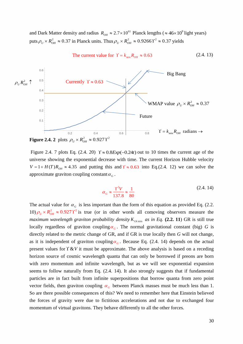
The current value for min0.63
OHk R (2.4. 13)
Figure 2.4. 2 plots 2 2
0.927U OH
R
Figure 2.4. 7 plots Eq. (2.4. 20) 0.8 ( 0.24 )Exp t out to 10 times the current age of the
universe showing the exponential decrease with time. The current Horizon Hubble velocity
1 ( ) 4.35OH
V H T R and putting this and 0.63 into Eq.(2.4. 12) we can solve the
approximate graviton coupling constant G .
2
1
137.8 80G
V
(2.4. 14)
The actual value for G is less important than the form of this equation as provided Eq. (2.2.
10)2 2
0.927U OH
R is true (or in other words all comoving observers measure the
maximum wavelength graviton probability density minGkK as in Eq. (2.2. 11) GR is still true
locally regardless of graviton coupling G . The normal gravitational constant (big) G is
directly related to the metric change of GR, and if GR is true locally then G will not change,
as it is independent of graviton coupling G . Because Eq. (2.4. 14) depends on the actual
present values for &V it must be approximate. The above analysis is based on a receding
horizon source of cosmic wavelength quanta that can only be borrowed if preons are born
with zero momentum and infinite wavelength, but as we will see exponential expansion
seems to follow naturally from Eq. (2.4. 14). It also strongly suggests that if fundamental
particles are in fact built from infinite superpositions that borrow quanta from zero point
vector fields, then graviton coupling G between Planck masses must be much less than 1.
So are there possible consequences of this? We need to remember here that Einstein believed
the forces of gravity were due to fictitious accelerations and not due to exchanged four
momentum of virtual gravitons. They behave differently to all the other forces.
0.2 0.4 0.6 0.8
0.1
0.2
0.3
0.4
0.5
0.6
2
U OHR
WMAP value 2
0.37U OH
R
Big Bang
Future
min radians
OHk R
Currently 0.63

31
2.4.3 Possible consequences of a small gravitational coupling constant
In quantum mechanics forces between charged particles are due to the exchange of virtual
bosons. All scattering crossections are calculated from the exchanged 4 momenum of these
bosons. General Relativity suggests that the forces of gravity are fictitious and only seem real
due to the change of the metric. This paper proposes that the change in the metric around
mass concentrations is consistent with keeping the “min
k Graviton Constant minGkK ” of Eq.
(2.2. 11) invariant. These changes in the metric are about 80 times greater than the coupling
constant suggests. We are suggesting in this paper that spin 2 gravitons only cause changes in
the metric by the need to keep min min minGk GkK dk invariant. The attempts to develop a
quantum field theory for gravitons have difficulty with the infinities at Planck energies that
are not renormalizable. They assume a gravitational coupling constant of one between Planck
masses. This could change if this coupling constant is in fact about 80 times smaller, as
Planck energy gravitons would no longer automatically form Black holes. However it may be
irrelevant if, as Einstein believed, gravity is not due to exchanged 4 momentum.
2.4.4 A possible exponential expansion solution and scale factors
Let the scale factor be a then density3
1
a and Eq. (2.2. 10) tells us the average density of
the universe
2
21.41
U
OHR
so that
2
2 3
1U
OH
KR a
where 1.41K is constant.
Thus 3 2 2 2/3 2/3
a KR a K R where OH
R R (2.4. 15)
The Hubble parameter H is
1/3 2/3 2/3 5/3
2/3 2/3 2/3 2/3
(2 / 3) (2 / 3) 2 1 1
3
dR dK R K Ra dR ddt dtHa K R K R R dt dt
2 Thus the Hubble Horizon velocity @ is
3OH
dR RR V H R
dt
d
dt
(2.4. 16)
We can also write Eq.(2.4. 14) 2164 a constant
GV , hence
22 0dV d V .
Thus 1
2
1dV
V dT
d
dT
and Eq. (2.4. 6) tells us that the Horizon velocity OHdR dR
Vdt dt
.
Equation (2.4. 6) also tells us that 1V H R V so we can write Eq. (2.4. 16) as
2 2
3( 1) 22
d
d
R R dVV
V ttV
d
3
R dVV
V dt ( 3)
dV VV
dt R
(2.4. 17)

32
We will look for an exponential increase of the horizon velocity so / 0dV dt and 3 .V
Let us try first a simple 3 ( )V Exp bt with 3V for all values of & 0b t .
Also simply put 0 0
3 ( )t t
R Vdt Exp bt dt thus 3[ ( ) 1]Exp bt
Rb
.
Putting this value for R plus 3 ( )V Exp bt & 3 3[ ( ) 1]V Exp bt into Eq. (2.4. 17)
( 3) 3 ( ) 3[ ( ) 31]3[ ( ) 1]
( )V b
V Exp bt Exp btR Exp b
dVbExp bt
d tt
.
But 3 ( )V Exp bt and again 3 ( ) 3 ( )dV d
Exp bt bExp btdt dt
. Thus Eq’s. (2.2. 10) & (2.4. 14)
are consistent with 3 ( )V Exp bt for positive b regardless of the value of graviton coupling G
A possible expansion solution is 3 ( )V Exp bt & 3[ ( ) 1]Exp bt
Rb
, 0.b
(2.4. 18)
But is this consistent with the local special relativity requirement for OHR ? In other words
does0
3[ ( ) 1]@ time ( )
( )
T dt Exp bTR T a T
a t b
? Now Eq. (2.4. 15) tells us the scale factor
3 2 2 2/3 2/3a KR a K R
but Eq.(2.4. 14) says2
1/V so the scale factor1/3 2/3
.a V R
From Eq. (2.4. 18) ignoring the constant factors 3 & b, ( )V Exp bt & ( ) 1R Exp bt
1/3 2/3
0
1/3 2/3
/3 2 3
0
1 /
The scale factor ( ) ( ) [ ( ) 1]
Thus ( )
=( ) [ ( ) 1]
3[ ( ) 1]
( )
( ) [ ( ) 1]
T
T
a t Exp b
a T
Exp bT E
t Exp bt
dtR
a t
dt
Exp bt Exp bt
Exp b
b
b
xp T
T
(2.4.19)
And Eq. (2.4. 18) appears to be a consistent exponential expansion for both V and R.
From Eq. (2.4. 14) we showed 1
2
1dV
V dT
d
dT
. Using Eq. (2.4. 18) 3 ( )V Exp bt &
3 ( )dV
bExp btdt
implies ( / 2)K Exp bt . The current value of 0.63 from Eq.(2.4.
13) and our best guess of 0.48b from Figure 2.4. 3 yields
min0.8 ( 0.24 ) in radians
OHk R Exp t
(2.4. 20)

33
Time t
0
0
0
Shaded Area
3 (0.48 )
3[ (0.48 ) 1]
0.48
( )( )
T
T
T
R Vdt
Exp t dt
Exp T
dta T
a t
Figure 2.4. 4
Time t
Figure 2.4. 5
0.48 is based on
1Hubble now
and is best guess.
b
T
Time t
0.8
0.5
0.3
b
b
b
Figure 2.4. 6
Hubble
b
Hubble parameter
1/H T now if 0.48b
always 2 / 3H t if 0b
Figure 2.4. 3

34
2.4.5 Possible values for b and plotting scale factors
This simple exponential expansion starts at the Big Bang and is very different to the current
cosmology models that keep a constant horizon velocity until Dark Energy starts to take
effect. This continuous exponential increase could well lead to slightly different values for
the radius OHR and also possibly the age 9
13.8 10T years. (Some recent observations [7]
have also been questioning the leading current dark energy explanations of acceleration).
Current cosmology models put the Hubble parameter as / 1/H a a T at present (based on 9
13.8 10T years). It also simplifies the plots above if we put 9
13.8 10 years 1T , with
OHR or radius R becoming multiples of 1T . Using Eq. (2.4. 6) 1 ( )V H T R , Figure 2.4.
3 plots the Hubble parameter by time ( 1)T now as a function of the exponential time
coefficient b showing if 0b that always 2 / (3 )H t as in current cosmology at critical
density with no dark energy. Also if 1/H T now the best guess is 0.48b . This yields
3.85R T or 15% greater than current cosmology. Figure 2.4. 4 plots horizon velocity &
Figure 2.4. 5 the scale factor based on 0.48b , but of course the actual value of b or rate of
change with time must be in agreement with the redshifts currently observed when looking
back towards the big bang. These could well change b and radius R. Figure 2.4. 6 plots the
transition to positive acceleration of the scale factor showing the effect of changing the value
of b. Figure 2.4. 7 plots Eq.(2.4. 20) min0.8 ( 0.24 )
OHk R Exp t out to 10 T.
2.5 An Infinitesimal change to General Relativity effective at cosmic scale
All we have discussed is based on the energy in the zero point fields being limited. We
argued that uniform mass density throughout the cosmos has mink graviton probability
density minGk as in Eq. (2.2. 11). At this probability density the zero point quanta density
available equals that required. To maintain this required balance as in Figure 2.4. 1 we argued
that around any mass concentration the curvature of space expands space locally so as to keep
the mink graviton constant min
0.262GGk
K as in Eq. (2.2. 11) invariant at all points. In other
words our conjecture only works if the local curvature of space depends on the difference
2 4 6 8 10
0.2
0.4
0.6
0.8
Figure 2.4. 7
Cosmic time t
0.63 radians now
Current time 1t
Big Bang

35
between the local mass density and the uniform background. Compared to General Relativity
this is an infinitesimal change except at cosmic scale. GR says the curvature of space depends
on local mass density whereas we argue that it depends on the difference between local mass
density and the average background (only a few hydrogen atoms per cubic metre). This
automatically guarantees the universe to be flat on average. All our aguments start with flat
space on average. The equations of GR would look almost identical except the Energy
Momentum Tensor T in comoving coordinates requires 00T the mass/energy density to
change from to U where the density of the universe U
is as in Eq.(2.2. 10).
00 In comoving cordinates changes from to in the Energy Momentum Tensor
UT T (2.5. 1)
2.5.1 Non comoving coordinates in Minkowski spacetime where g
To this point everything we have looked at has been in comoving coordinates. Velocities
relative to comoving coordinates are usually referred to as peculiar velocities, so, does what
we are saying above still apply in such non comoving coordinates? In section 2.3.1 we said
that spin 1 sources are 4 currents, but spin 2 graviton sources are the stress tensor. We have
also been saying up to here that the background mink gravitons are spherically symmetric or
time polarized in comoving coordinates. We are going to conjecture that in non rotating
Minkowski spacetime they are always time polarized, regardless of peculiar velocities. This
may seem impossible, as we would intuitively expect something to not remain spherically
symmetric if we move relative to it. But we are not talking about real particles; we are talking
about virtual spin 2 gravitons. We cannot see them, or detect them directly in any way, only
their consequences. We can calculate amplitudes and probabilities for their presence only. So
let us look again at these background mink graviton amplitudes and probabilities. In section
2.1.2 we found in Eq.(2.1. 10) the probability density of background mink virtual gravitons
2
Universe Universe min min min min 4
min
0.3056* where U
Gk Gk Gk
GK dk Kk
in comoving coordinates.
If we move relative to this at peculiar velocity P , measured volumes shrink as
1 2 1/2(1 )
P P
and all comoving mass increases as 2 1/2
(1 )P P
. (We will use red
symbols with the subscript P, and triple primes for wavenumber mink for peculiar velocities, to
distinguish them from metric changes where we used green and a double primed mink .) Thus
2
U P U .The minimum wavenumber min
k has its lowest value in comoving coordinates (at
least far from mass concentrations where g ) but at peculiar velocity P , mi minn P
k k .
2 4
4 4
2 2
min4 4
min mimi nn
and is invariant.U UU P
P
Gkkk
Kk
min min minGk GkK dk in non comoving coordinates if g
(2.5. 2)

36
2.5.2 Non comoving coordinates when g
Starting with Eq. (2.1. 10) min min minGk GkK dk we have just shown that this equation remains
true at any peculiar velocity P in flat spacetime. All that happens is that the values of min
k ,
mindk & min min minGk Gk
K dk all increase as 2 1/2
(1 )P P
. In other words the probability
of finding a mink graviton is always proportional to whatever the value min
k &min
dk is. Also the
amplitude to find a mink graviton is always proportional to either
mink or
mindk . We have
shown in sections 2.1 & 2.2 that around mass concentrations in comoving coordinates, the
mink gravitons are comprised of the background due to the universe plus the interaction
between the local mass and the universe as in Figure 2.2. 2 . This background mink graviton
probability, regardless of the local metric, is always proportional to whatever the local value
mink & min
dk is. Amplitudes are also always proportional to local values of min
k or min
dk .
minAmplitude (due to rest of universe)
Gk or Universe min
allways dk (2.5. 3)
As in Figure 2.2. 1 the probability for a small mass m to emit a mink graviton is
2 min
min
2G
dkm
k
.
The normalized wavefunction min2min min min
2 2 2
2 2 2 3.556
4 4 4
k rk k ke
r r r
minas 0k r & min min
3.556k k
using Eq. (2.1. 4). Thus we can say the:
2
min
minmin min
2 2
min
3.5563.5562Amplitude (due to small mas
2s
2
4 )
G Gk
Gdkdk k m
mk r r
m
min
2
3.5562=
4
m
Gdkm
r
is allways
min
2mdk
r
(2.5. 4)
The interaction between this small mass and the rest of the universe is
Universe Universe mimin m nminn i
2 + is allw* * ays
2Gk m m
m mdk
rddk k
r .
We have shown previously that minGkK is the proportionality constant. So regardless of
peculiar velocities
Universe Univmin min merse in + is allways
2* *
mG Gmk k
mK dk
r
(2.5. 5)
Thus Universe Universemin* * +
m mGk is always proportional to min
dk and at peculiar
velocity P ; mi minn P
k k & min minPkdk d . So both min min
&Gk Gk
increase as P and their
ratio does not change. The logic of our aguments is not affected by peculiar velocities. The
same is true for large masses moving at peculiar velocities. In a metric M as in section 2.2.2
(using four blue primes for combined peculiar velocity and metric changes) min minMPk k

37
and n mimi nMPd kk d . Both min min
&Gk Gk
increase as P
M and again their ratio does not
change. All the arguments we used in section 2.2.2 do not change and Equ’s. (2.2. 14), (2.2.
15) & (2.2. 16) still apply in non comoving coordinates providing M is the velocity reached
by a small test mass falling from infinity in the same rest frame as the mass concentration m
moving at peculiar velocity P . We can think of min
0.262GGk
K as a constant scalar
throughout the universe representing the Probability Density of finding a minimum
wavenumber min minMPk k virtual graviton at all points of spacetime. Near mass
concentrations the metric changes; local clock rates change, and so does the measurement of
mink , but not the scalar minGk
K . Locally measured infinitesimal volumes increase to
accommodate the extra locally emitted maximum wavelength gravitons keeping the scalar of
probability density constant. We argue that General Relativity is consistent with this. If we
think of the mass in the universe as a dust of density U essentially at rest in comoving
coordinates we can define a tensor (Background)T . In comoving coordinates
(Background)T has only one non zero term 00(Background)
UT . In any other coordinates
this same (Background)T tensor is transformed by the usual tensor transformations that
apply in GR. If these coordinates move at peculiar velocityP
then 2
00(Background)
P UT
2
00(Background)
PT . This all suggests the infinitesimally modified Einstein field equations
4
1 8(Background)
2
GG R g R T T
c
(2.5. 6)
We argue that Eq. (2.5. 6) is consistent with keeping the scalar min0.262
GGkK constant
throughout all spacetime as in Figure 2.5. 1. This infinitesimal modification is only relevant
in the extreme case as T approaches (Background)T . Far from mass concentrations
(Background)T T . Space curvature, in these remote voids, is in general somewhere
between slightly negative and zero; but the causally connected universe is flat on average
regardless of the value of . .
minGk
G
K
mink
min0.1 0.25k
very approximately
@ the Big Bang
62
min10k
now
At any cosmic time T in any coordinates, and in any metric,
in the infinitesimal band mindk , min min minGk Gk
K dk is always
true. minGkK is a constant scalar, but the measurement of min
k
depends on both local metric clockrates and cosmic time T .
Future
Figure 2.5. 1 Past
38
If there is no inflation, in comoving coordinates, at the Big Bang or slightly after, min
k starts at
just under one and is always close to the inverse of the causally connected horizon radius. It
is also close to the inverse of cosmic timeT . It is always at its minimum far from mass
concentrations, but increases with the slower clock rates in the local metric around mass
concentrations as in Figure 2.5. 1
2.5.3 Is inflation in this proposed scenario really necessary?
There are two main reasons, usually given, for why inflation is necessary:
(a) The average flatness of space.
(b) The almost uniform temperature of the cosmic microwave background from regions that
were initially out of causal contact.
If we put (Local) (Background)T T in Eq. (2.5. 6), the right hand side is identically zero,
and 1
02
G R g R on average throughout all space. The average curvature of all
space must be zero and space is compelled to be flat on average.
In section 2.4.4 we found that space naturally expands exponentially as in Eq.(2.4. 18) and
plotted in Figure 2.4. 4. The value of the constant b in 3 ( )V Exp bt has to fit experimental
observations. But if it is some fundamental constant, which does not seem unreasonable, it
must be the same for all comoving observers. If this is so the physics is identical for all such
observers regardless of whether they are in causal contact. Provided we can assume identical
starting points everywhere, of say the Planck temperature at cosmic time 0T , then apart
from quantum fluctuations, the average background temperature should be some function of
cosmic time T for all comoving observers, or at least up to the time the universe became
transparent. The physics controlling this should be identical in each comoving frame. Causal
contact should not be essential for this. Inflation only guarantees that the starting temperature
is uniform everywhere when it stops at approximately 0.T It also has to assume identical
physics everywhere from 0T for about the first 375,000 years, or untill the universe is
transparent. This is virtually identical to what we are proposing in our scenario.
2.5.4 Why do we think virtual particle pairs do not matter?
This topic is discussed more fully in the first paper [7] on pages 85 & 86. A shortened
summary goes a bit like this: Virtual particle pairs by definition only last briefly. Zero point
energies are limited mainly for times similar to the age of the universe. The conservation of
energy or in reality 4 momentum says that what we call “real matter or energy” can last for
close to the age of the universe. It will have mass and by definition it can be weighed. It can
move around, even close to the speed of light, but it is conserved. Gravitons that last this long
we have called mink gravitons and they can only couple to real, or long lasting energy/matter
that can be weighed in whatever manner. The rotating dark matter in galaxies we cannot

39
weigh directly, but it contributes to the theoretical weight of a galaxy. We have to allow for
this mass when studying galaxy dynamics. The gluons that bind quarks are virtual, and form
the bulk of nuclear mass and all normal matter. They are virtual particles, but protons appear
to last for at least the age of the universe. They must couple to long lasting min
k gravitons.
We cannot weigh the virtual particle pair background. It may have huge consequences in
quantum field theory, and we can measure these effects very accurately, but they are all due
to very brief events. We argue however that they do not couple tomin
k gravitons. If they
somehow did, the total number of min
k gravitons would be so vast it would completely
outstrip (by about 12010 ) the supply of min
k quanta supply from the holographic horizon.
2.6 Messing up what was starting to look promising, or maybe not
2.6.1 The kmin virtual gravitons emitted by the mass interacting with itself
In section 2 we started out by finding the average mink graviton probability density in a
uniform universe. We then placed a mass concentration in it and calculated the extra
probability density of mink gravitons (before the dilution due to local space expansion) due to
the amplitude of this mass by the amplitude of the rest of the mass in the universe. This ended
up being proportional to /m r in Planck units.
min Universe Universe( * ) ( * ) /
Gk m mm r as in Eq.(2.2. 6)
And this is true in weak field metrics, except as we start approaching the Schwarzchild
Radius because of the extra mink gravitons from the mass interacting with itself: *
m m .
Using Eq. (2.1. 5)
2 2
2 2*
r
m m G
km k e dk
r k
Also using Eq. (2.1. 4)2 2
min min11.644 3.556k k k k when min
k k
min2(3.556 )2
min min
2 2
min
3.556*
G
k r
m m
k e dkm
r k
The exponential term m i n m i n2 ( 3 . 5 5 6 ) 7 . 1 1 22 k r k rk re e e
and we are only interested in
radii r that are small in relation to the observable radius of the Universe 1
minOUR k
, just as
in the assumptions we made in section 2.2.1. Thus 0k r and 21
k re
in these regions so
we can approximate this equation as
2
min2 2
3.556*
Gm m
mdk
r

40
2
min min2 due to self emission * 0.36
k m GG m
mdk
r
2
min21.375 0.262
G
mdk
r
2
min min21.375
Gk
mK dk
r using Eq.(2.2. 11)
If the local clock rate is 00
1
M
g
as in Eq.(2.2. 13) but with a slightly modified 00
g (as
we will see below), before dilution due to the local space expansion we can measure:
Before dilution minGk due to *
m m
2
2
min min21.375
M Gk
mK dk
r
(2.6. 1)
2.6.2 What does this extra term mean for non rotating black holes?
When deriving Eq.(2.2. 14) we found (about two equations previous) that due to interactions
with the rest of the Universe min min min mi
2 2
n
2 0.262 2
Gk GkM MG
m mdk K dk
r r
2
min min mi2
2
nThus total 2 1.375
Gk GkM
m mK dk
r r
in Planck units.
(2.6. 2)
Staying on our current path appears to contradict General Relativity, but temporarily ignoring
this, let us repeat section 2.2.2 which modifies a non rotating black hole metric to
2
00 2
1 21 1.375
rr
m mg
g r r
2
2
2
2
2 2
21.375
1
1 2 / 1.375 /
M
M
m m
r r
m r m r
(2.6. 3)
Where M is the velocity reached by a small test mass falling in from infinity in the same
rest frame. Applying the same proceedures as in section 2.2.2 we can use Equ’s. (2.6. 3) to
show that min min minGk GkK dk in this new metric, and we will discuss possible tensions with
General Relativity in section 2.6.5. The modified non rotating horizon radius occurs when
2 22 1.375 0r mr m or the:
Modified non rotating horizon radius 2.54r m (2.6. 4)
This is approximately 27% larger than the Schwarzchild value.
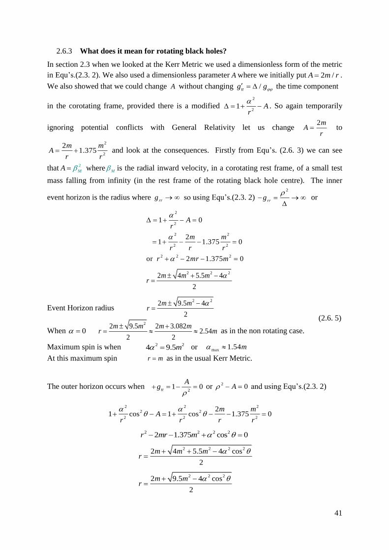
41
2.6.3 What does it mean for rotating black holes?
In section 2.3 when we looked at the Kerr Metric we used a dimensionless form of the metric
in Equ’s.(2.3. 2). We also used a dimensionless parameter A where we initially put 2 /A m r .
We also showed that we could change A without changing /tt
g g the time component
in the corotating frame, provided there is a modified 2
21 A
r
. So again temporarily
ignoring potential conflicts with General Relativity let us change 2m
Ar
to
2
2
21.375
m mA
r r and look at the consequences. Firstly from Equ’s. (2.6. 3) we can see
that2
MA where M
is the radial inward velocity, in a corotating rest frame, of a small test
mass falling from infinity (in the rest frame of the rotating black hole centre). The inner
event horizon is the radius where rrg so using Equ’s.(2.3. 2)
2
rrg
or
2
2
2 2
2 2
2 2 2
1 0
2 1 1.375 0
or 2 1.375 0
Ar
m m
r r r
r mr m
2 2 2
2 4 5.5 4
2
m m mr
Event Horizon radius 2 2
2 9.5 4
2
m mr
When 0 2
2 9.5 2 3.0822.54
2 2
m m m mr m
as in the non rotating case.
Maximum spin is when 2 24 9.5m or max
1.54m
At this maximum spin r m as in the usual Kerr Metric.
(2.6. 5)
The outer horizon occurs when 2
1 0tt
Ag
or 2
0A and using Equ’s.(2.3. 2)
2 2 2
2 2
2 2 2
21 cos 1 cos 1.375 0
m mA
r r r r
2 2 2 22 1.375 cos 0r mr m
2 2 2 2
2 4 5.5 4 cos
2
m m mr
2 2 2
2 9.5 4 cos
2
m mr

42
2 2
2
2 9.5 4Ergosphere radius @ 0 &
2
2 9.5 2.54 @
2 2
m mr
m mm
(2.6. 6)
Figure 2.6.1 Modified Kerr Metric with the dimensionless parameter A changed from
2mA
r
2
2
21.375
m mA
r r . (This conflicts with General Relativity near the horizon.)
Figure 2.6. 2 Spinning black hole mass m with angular momentum length parameter , but
with the dimensionless parameter A changed from 2m
Ar
2
2
21.375
m mA
r r . The
determinant of the metric is independent of A. The denominator terms &g g , in
dimensionless form as in Equ’s. (2.3. 2), rapidly tend to one, as does2
M for radii Sw
r r ,
and can be ignored.
Time polarized mink graviton extra probability density
outside sphere varying as
2
2
2
21.375
M
m m
r r
g
Spin Axis
Circularly polarized 2m mink graviton extra
probability density varying as 2
2 2
2cos
Mr
Transversely polarized 2m mink graviton extra probability
density varying as
2 2
2
2 2
2
21.375 sin
M
m m
r r r
g g
Event Horizon r m @ maximum spin is same as Kerr
Metric, but maximum spin has increased by 54% .
Ergosphere maximum radius 2.54r m is
the same as a modified non-spinning black
hole.

43
Figure 2.6.1 illustrates these changes from the Kerr Metric. The main effect from changing A
is to allow an increase in maximum spin from m to 1.54m , and an 27% increase in
the maximum ergosphere radius from 2 to 2.54mr m . It may appear to contradict General
Relativity, but provided the extra densities of time, 2m circular and transverse polarized
mink gravitons are as in Eq.(2.3. 7) with
2
2
21.375
m mA
r r then
min min minGk GkK dk is still
true in the rotating space outside the black hole.
Figure 2.6. 2 shows the probability densities of time polarized, circular and transverse
polarized 2m min
k gravitons as in Eq.(2.3. 7) in this modified metric before the
expansion of space, which dilutes the probabilies so as to keep the min
k graviton constant
minGkK invariant outside the black hole.
2.6.4 The determinant of the metric and the min
k graviton constant minGkK
In a corotating rest frame the metric can be written in diagonal form, as in this frame 0d
dt
.
Working in dimensionless form as in Equ’s.(2.3. 2) and using Eq. (2.3. 3)tt
gg
but
ignoring signs we have 2 2
2 4 2 2
2(1 cos )
rr ttg g g g g
g r
In dimensionless form the Determinant of 2
4 2 2
2(1 cos )g
r
It is independent of the dimensionless parameter .A
(2.6. 7)
Despite possible conflicts with General Relavity, if the determinant of the metric in a
corotating frame is as in Eq. (2.6. 7) or always 4 then the mink graviton probability density is
min min minGk GkK dk at all points outside the rotating black hole, and this is also true if there is
no rotation.
2.6.5 General Relativity is based on mass not mass squared
It would appear that including the self interaction term *m m
, with its introduction of an 2 2
/m r term in the metric, does not naturally relate with General Relativity where the Stress
Tensor has 00T based on mass/energy densities, with no mass squared terms. But if our
hypothesis that min min minGk GkK dk is to be always true, and we include the *
m m term then
we are forced to accept an 2 2/m r term in the metric. The match between an invariant min
k
graviton constant minGkK , and an infinitesimally modified General Relativity as in Eq.(2.5. 6)
4
1 8(Background)
2
GR g R T T
c
is remarkably accurate from close to black
holes to near the cosmic horizon. But not very close to black holes if we include *m m
.

44
Einstein based his remarkable equation on the Equivalence principle (the same physics in all
free falling frames as in empty space) and the covariant derivative behaving correctly in all
coordinates and throughout all spacetime. His thinking went along similar lines to Gauss’s2 , but in curved spacetime. This naturally leads to inverse square force laws with
inverse potentials, but the inclusion of an 2 2/m r potential term in the metric due to *
m m
seems to mess all this up. But does it really? Or alternatively, could it be trying to tell us
something that we did not want to know, but need to know?
Quantum mechanics in the form of QED tells us that close to fundamental electric charges
Gauss’s inverse square force law breaks down and QED takes over with almost unbelievable
accuracy. The inverse square electric force law had ruled with remarkable accuracy for over a
century before QED arrived on the scene. In fact it was the announcement of the Lamb Shift
at the Long Island conference in 1947 that started the big breakthroughs in QED. World War
II developments in radar had enabled these remarkably accurate experiments. Is it possible
that similar developments today will allow improvements in Gravitational Wave observation
accuracy? Developments that may see effects in gravity close to black hole horizons with
some parallels to those of QED close to electric charges?
2.6.6 Frame Dragging has to occur in this proposed scenario
Lense and Thirring [25] were the first to show that General Relativity predicted this about
two years after Schwarzchild’s solution to Einstein’s field equations. And of course the Kerr
metric exact solution for rotating black holes also confirms it. In section 2.2.2 we showed that
the Schwarzchild metric near large non-rotating masses is consistent with the mink graviton
constant minGkK as in Eq. (2.2. 11) remaining constant. This metric tells us that, as seen from
a large distance, time at the horizon of a black hole stops, and the velocity of light drops to
zero. Photons and gravitons are frozen in place. We have argued that the extra mink gravitons
near the horizon, due to this mass, cause this warping of spacetime that freezes time on the
horizon. This effectively locks spacetime to mass on that horizon. The extra mink gravitons
just above the horizon can be thought of as due to the adjacent mass immediately below
them, and in section 2.6.1 we addressed the affect of this *m m
self emission. So if space
time just above the horizon is locked to non-rotating black hole mass, it must also be locked
to the moving mass of a rotating black hole. We are of course assuming here that, as pointed
out in the first paper, infinite superpositions cannot exist inside the horizon. This suggests the
horizon might be a spacetime boundary consisting of a few Planck thicknesses of
exponentially decreasing Planck density mass. This also implies that the Equivalence
Principle could possibly breakdown near the horizon if these arguments involving infinite
superpositions are true. In normal General Relativity this breakdown in the laws of physics is
seen to occur at the central singularity. The breakdown has to happen somewhere in this
region, either at the centre or, as we suggest, it has to be the horizon [19] [20] [21] [22] [23].

45
2.7 Revisiting some aspects of the first paper that we have now modified
2.7.1 Infinitesimal rest masses
This was covered in the first paper but there are some small corrections as we had used the
expectation value of the superposition number n when we should have used 2n . Also
small corrections we have made in the expansion of the universe have changed the value of
min OHk R in Eq. (2.2. 10) from 0.51 to 0.63 . From Table 4.3.1 page 61 in the first
paper we find that for spin 1 24.095n and for spin 2 2
3.41n . Using these new
values and 0.63 we can redo Table 6.2.1 on page 84 of the first paper [7]. (These
changes increase infinitesimal rest masses approximately 20% compared with the first paper.)
Spin 2
n Compton Wavelength c Infinitesimal Rest Mass
1 4.095 0.58OH
R 347.8 10 .eV
2 3.41 0.49OH
R 349.3 10 .eV
Table 2.7. 1 Infinitesimal rest masses of 2N photons, gluons and gravitons.
2.7.2 Redshifted zero point energy from the horizon behaves differently to local
Local zero point energies are Lorentz invariant. At high frequencies there is no shortage
locally to build the high frequency components of superpositions. If a massive 1N virtual
pair emerges from the vacuum its life is short and it places little demand on long range
quanta. If there were no redshifted supply from the horizon there would be only a few modes
of the local supply of min1 /
OUk R quanta inside the horizon. Because preons are born with
zero momentum and infinite wavelength they can however absorb a different supply of
redshifted min1 /
OUk R quanta from the receding horizon as we have discussed. This min
k
quanta redshifted supply behaves differently to normal Lorentz invariant zero point local
fields. It behaves as min min
1.745 "The Quanta required @ Constant"Qk G
K k of Eq. (2.4. 12)
Where min min min
6.66 "The Graviton Constant"Qk Gk
K K k of Eq. (2.2. 11).This redshifted supply
is only available to preons that are born with zero momentum, or infinite wavelength, in the
rest frame in which infinite superpositions are built.
2.7.3 Revisiting the building of infinite superpositions
In section 2 of the first paper we developed equations to determine the probability of each
mode of a superposition using local zero point fields and in section 2 when we found the

46
cosmic wavelength supply inadequate we switched to a different redshifted supply for long
range quanta. So how do we justify our use of the local zero point fields to determine mode
probabilities and behaviours? There is simply a plentifull supply of high frequency local zero
point fields. This local supply is adequate for high densities of superpositions for all modes
from the Planck energy 1k high energy mode cutoffs to somewhere around 2010k
or
near nuclear wavelengths. Thus until we reach somewhere hear nuclear densities there is a
sufficient supply of local high frequency zero point fields to build infinite superpositions. The
coupling to local zero point fields in this high frequency region determines the behaviour of
all the standard model particles. There is however a gradual transition to absorbing quanta
from the redshifted horizon supply as the wavelength increases. Because the redshifted
supply of mink quanta behaves as the invariants
min minor
Qk GkK K above and entirely differently
to Lorentz invariant local zero point fields, spacetime has to warp around mass concentrations
and the universe has to expand.
2.8 Gravitational Waves
Our hypothesis has been throughout, that the warping of spacetime is directly related to
maintaining the maximum wavelength, or mink graviton density min min minGk Gk
G dk invariant
throughout all spacetime. Around non-rotating (spherically symmetric) mass concentrations
this warping decreases inversely with radius (at least well away from black holes) but always
in a spherically symmetric manner as the extra mink gravitons due to this mass are distributed
in the same spherical way. Likewise we get cylindrical symmetry for rotating mass
concentrations. Both these types of symmetries are the lowest energy stable state of the
metric. Disturbances to this stable state will travel as waves at the speed of light.
2.8.1 Constant transverse areas in low energy waves
If these mass concentrations accelerate, then just like accelerating electric charges they will
radiate gravitational energy in the form of real transversely polarized min2,m k gravitons.
This energy is a disturbance or oscillation in this lowest energy state mink graviton
background, but min min minGk GkG dk cannot change during these disturbances, so what is
going on? Let us imagine a region of spacetime far from mass concentrations where the
metric g and using , , ,t x y z coordinates let 00
1, 1, 1, 1.xx yy zz
g g g g
Ignoring signs the determinant of the metric 1g . Let a gravitational wave pass through
in the z direction with a tranverse wave in the ,x y plane. We know that a circular transverse
ring of particles will oscillate into and out of ellipses perpendicular to each other, in such a
manner that the enclosed area does not change, or that 1xx yy
g g during this oscillation.
Thus the measured volume of space does not change as the wave passes through and
min min minGk GkG dk does not change. The determinant of the metric 1g also does not
change. This is only approximately true as there are extra real transversely polarized

47
min2,m k gravitons passing through due to the energy in the wave, but the error is second
order unless the amplitude of the wave is quite large.
2.8.2 What happens in high energy waves?
We can imagine the extra gravitons around a mass concentration and the background
gravitons as in section 2.2 (if they are undergoing an acceleration as in binary pairs)
generating real transversely polarized 2m gravitons of the same wavenumbers. (This has
some parallels to what we found in the Kerr metric, but now with real gravitons.) The
intensity, or probability density, of these real gravitons will drop as the inverse radius
squared. We can also show from Equ’s.(2.1. 9) &(2.2. 5) that most of these gravitons are
close to mink wavenumber. About 66% between min
k & 2 mink and about 96% between min
k &
5 mink . Thus most of this radiated energy is near min
k . Just as measured volumes around mass
concentrations had to increase to accommodate extra mink gravitons, the transverse area of the
wave has to increase very slightly in relation to the oscillating constant area. Ignoring signs
again 1xx yy
g g so 001g to keep the metric determinant 1g . The small energy
density in the wave increases infinitesimally the local measurement of mink , thus allowing
min min minGk GkG dk to remain invariant as required. Close to orbiting binary black holes or
neutron stars this radiated energy intensity is huge and the changes in 00
&xx yy
g g g become
large in relation to the oscillating changes. Transverse areas and hence measured volumes
change significantly. This is in complete contrast to what happens at large distances, such as
when we observe gravitational waves here on Earth, where the transverse areas are virtually
constant during these oscillations.
2.8.3 No connection between wave frequency and radiated quanta energy
The frequency of the radiated wave is twice the orbital frequency of the binary pair source.
As most of the energy in the wave is in quanta near mink there is no connection with the
frequency of the radiated wave as in spin 1 photons in electromagnetism. In the recently
observed gravitational waves the wave frequency was 250 cycles per second just before
merger with wavelengths 1200 kilometres or approximately 4110 Planck lengths, whereas
the wavelength of mink gravitons is 62
min1/ 10
OUk R Planck lengths. The ratio between
them is 2110 . This ratio is inverse to the binary pair orbital frequency. It could only
approach one if the orbital period is approximately twice the age of the universe.

48
3 Conclusions
If the fundamental particles can be formed from infinite superpositions as outlined in the first
paper our hypothesis is that the warping of spacetime is directly related to maintaining the
maximum wavelength, or min
k graviton density min min minGk Gk
G dk invariant throughout all
spacetime. Thinking in a simple way and using the proportionality symbol as follows:
In a universe with no mass concentrations Universe Universmin e
( * )Gk
. With a concentration
of mass m , UnUniverse Univers iverse Universemi en
( * * )* ( *) )(m mm mGk
but space
expands locally to restore minGk
back to min min minGk Gk
G dk . The green term
Universe Universe( * * )
m m requires 2 /m r in the metric, and blends well with an
infinitesimally modified General Relativity. This modification changes the 00T component
from 00T , where is the local mass density, to
00 UT , where
U is the average
density of the Universe (only a few hyprogen atoms per cubic metre). It matches the
Schwarzchild metric, and can fit the Kerr metric. In the first paper we focused only on this
term to illustrate a possible connection with quantum mechanics, provided the fundamental
particles can be made from infinite superpositions borrowing energy from zero point fields.
This second paper messes up that nice connection by introducing the troublesome blue term
( * )m m
with its associated 2 2/m r in the metric. This does not seem to relate with mass
densities in Einstein’s stress energy tensor. It may not however alter the event horizon radius
of a maximum spin black hole, but does seem to allow about 54% more spin. These values as
with other findings are only approximate however, as for simplicity we assumed a square
cutoff at min.k An exponential cutoff is most likely and will no doubt change these values,
especially the coefficient of the 2 2/m r term in the metric due to ( * )
m m . But if our
conjecture is true this term will not go away. So regardless of these approximations, as most
black hole mergers are between high spin black holes, this extra term may change the fine
details of the last few cycles. Testing this has to await future accuracy improvements in
gravitational wave detectors. It may show up in the fine details of spinning neuton star
collapse. It may also raise the possibility that there could be a parallel with the breakdown of
the inverse square law for fundamental charges near the Compton wavelength. Does General
Relativity hold all the way through the horizon as is normally thought? Most physicists
believe that it breaks down at the central singularity and an infalling observer sees no change
as they pass the horizon. However this clashes with both the Firewall paradox and the
Information paradox [19] [20] [21] [22] [23]. This paper suggests that there may well be
other reasons to question the current orthodoxy of the central singularity breakdown?

49
4 References
[1] A. Einstein, “The Foundation of the General theory of Relativity” (1916) Annalen Phys,
49:769-822
[2] D. Germanis, “General Relativity and Modified Gravity,” September 2011 and references
therein. https://workspace.imperial.ac.uk
[3] R. Jackiw, S.Y.Pi, “Chern-Simons Modification of General Relativity” (2003)
arXiv:gr-qc/0308071v2
[4] U.Ertem, “Generalized Chern-Symons Modified Gravity in First-Order Formalism”
(2009), arXiv:0912.1433v1
[5] C. Brans and R.H. Dicke, “Mach’s Principle and a Relativistic Theory of Gravitation”,
Phys. Rev. 124, 925 (1961).
[6] Carl Brans, “Invariant Approach to the Geometry of Spaces in General Relativity,” Jour.
Math. Phys., 6 94 (1965)
[7] J.Williams, “Exploring the Possibility of New Physics: Quantum Mechanics and the
Warping of Spacetime”, viXra:1303.0029v6
[8] De Rham, C., Gabadadze, G. & Tolley, A.J. Phys. Rev. Lett. 106, 231101 (2011)
[9] De Rham, C., Gabadadze, G., Heisenberg, L. & Pirtskhalava, D. Phys. Rev.D83, 103516
(2011)
[10] J.C. Pati, A. Salam, Phys. Rev. D10, 275 (1974).
[11] See for example H. Terazawa, K. Akama, Phys. Lett. B96, 276 (1980) and references
therein.
[12] H. Harari, Phys. Lett. B86, 83 (1979).
[13] M. Shupe, Phys. Lett. B86, 87 (1979).
[14] A. Rae, “Quantum Mechanics 3rd
edition”, (Institute of Physics Publishing, Bristol,
1992).

50
[15] R. Feynman, “The Feynman Lectures on Physics.” Volume III. (Addison Wesley,
Reading, Massachusetts, 1964).
[16] I. Aitchison, A. Hey, “Gauge Theories in Particle Physics, 2nd
edition”, (Institute of
Physics Publishing, Bristol, 1989).
[17] Cosmological Constraints from Measurements of Type 1a Supernovae discovered during
the first 1.5 years of the Pan-STARRS 1 Survey. arXiv:1310.3828
[18] W.G. Unruh, “Notes on Black Hole Evaporation,” Phys. Rev.D14 (4):870892 (1976).
[19] D. Marolf and J. Polchinski, Phys. Rev. Lett. 111, 171301 (2013).
[20] A. Almheiri, D. Marolf, J. Polchinski, and J. Sully, Journal of High Energy Physics.
2013, No. 2, 063 (2013).
[21] K. Papadodimas and S. Raju, “An infalling Observer in AdS/CFT” arXiv:1211.6767
(2012)
[22] R. Bousso, “Frozen Vacuum” arXiv:1308.3697 (2013)
[23] J. Maldacena and L. Susskind, “Cool Horizons for Entangled Black Holes”
arXiv:1306.0533 (2013)
[24] Maldacena, Juan (1998). "The Large N limit of superconformal field theories and
supergravity". Advances in Theoretical and Mathematical Physics. 2: 231–252. arXiv:hep-
th/9711200 .
[25] Lense, J.; Thirring, H. (1918). “On the Influence of the Proper Rotation of Central
Bodies on the Motions of Planets and Moons According to Einstein's Theory of Gravitation”
Physikalische Zeitschrift. 19: 156–163. Bibcode:1918PhyZ...19..156L.