Embed Size (px)
Citation preview

Alexander J. Smola: Exponential Families and Kernels, Page 1
Exponential Families and KernelsLecture 1
Alexander J. [email protected]
Machine Learning ProgramNational ICT Australia
RSISE, The Australian National University

Outline
Alexander J. Smola: Exponential Families and Kernels, Page 2
Exponential FamiliesMaximum likelihood and Fisher informationPriors (conjugate and normal)
Conditioning and Feature SpacesConditional distributions and inner productsClifford Hammersley Decomposition
ApplicationsClassification and novelty detectionRegression
ApplicationsConditional random fieldsIntractable models and semidefinite approximations
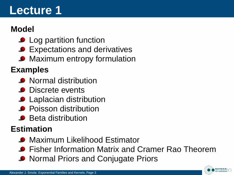
Lecture 1
Alexander J. Smola: Exponential Families and Kernels, Page 3
ModelLog partition functionExpectations and derivativesMaximum entropy formulation
ExamplesNormal distributionDiscrete eventsLaplacian distributionPoisson distributionBeta distribution
EstimationMaximum Likelihood EstimatorFisher Information Matrix and Cramer Rao TheoremNormal Priors and Conjugate Priors

The Exponential Family
Alexander J. Smola: Exponential Families and Kernels, Page 4
DefinitionA family of probability distributions which satisfy
p(x; θ) = exp(〈φ(x), θ〉 − g(θ))
Detailsφ(x) is called the sufficient statistics of x.X is the domain out of which x is drawn (x ∈ X).g(θ) is the log-partition function and it ensures that thedistribution integrates out to 1.
g(θ) = log
∫X
exp(〈φ(x), θ〉)dx

Example: Binomial Distribution
Alexander J. Smola: Exponential Families and Kernels, Page 5
Tossing coinsWith probability p we have heads and with probability 1−p we see tails. So we have
p(x) = px(1− p)1−x where x ∈ {0, 1} =: X
Massaging the math
p(x) = exp log p(x)
= exp (x log p + (1− x) log(1− p))
= exp(〈(x, 1− x)︸ ︷︷ ︸
φ(x)
, (log p, log(1− p))︸ ︷︷ ︸θ
〉)
The Normalization Once we relax the restriction on θ ∈ R2
we need g(θ) which yields
g(θ) = log(eθ1 + eθ2
)

Example: Binomial Distribution
Alexander J. Smola: Exponential Families and Kernels, Page 6

Example: Laplace Distribution
Alexander J. Smola: Exponential Families and Kernels, Page 7
Atomic decayAt any time, with probability θdx an atom will decay inthe time interval [x, x + dx] if it still exists. Consultingyour physics book tells us that this gives us the density
p(x) = θ exp(θx) where x ∈ [0,∞) =: X
Massaging the math
p(x) = exp(〈 −x︸︷︷︸
φ(x)
, θ〉 − − log θ︸ ︷︷ ︸g(θ)
)

Example: Laplace Distribution
Alexander J. Smola: Exponential Families and Kernels, Page 8

Example: Normal Distribution
Alexander J. Smola: Exponential Families and Kernels, Page 9
Engineer’s favorite
p(x) =1√
2πσ2exp
(− 1
2σ2(x− µ)2
)where x ∈ R =: X
Massaging the math
p(x) = exp
(− 1
2σ2x2 +
µ
σ2x− µ2
2σ2− 1
2log(2πσ2)
)= exp
(〈(x, x2)︸ ︷︷ ︸
φ(x)
, θ〉 −(
µ2
2σ2+
1
2log(2πσ2)
)︸ ︷︷ ︸
g(θ)
)
Finally we need to solve (µ, σ2) for θ. Tedious algebrayields θ2 := −1
2σ−2 and θ1 := µσ−2. We have
g(θ) = −1
4θ2
1θ−12 +
1
2log 2π − 1
2log−2θ2

Example: Normal Distribution
Alexander J. Smola: Exponential Families and Kernels, Page 10
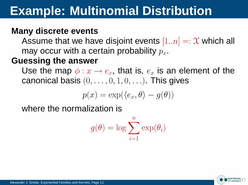
Example: Multinomial Distribution
Alexander J. Smola: Exponential Families and Kernels, Page 11
Many discrete eventsAssume that we have disjoint events [1..n] =: X which allmay occur with a certain probability px.
Guessing the answerUse the map φ : x → ex, that is, ex is an element of thecanonical basis (0, . . . , 0, 1, 0, . . .). This gives
p(x) = exp(〈ex, θ〉 − g(θ))
where the normalization is
g(θ) = log
n∑i=1
exp(θi)

Example: Multinomial Distribution
Alexander J. Smola: Exponential Families and Kernels, Page 12

Example: Poisson Distribution
Alexander J. Smola: Exponential Families and Kernels, Page 13
Limit of Binomial distributionProbability of observing x ∈ N events which are all in-dependent (e.g. raindrops per square meter, crimes perday, cancer incidents)
p(x) = exp (x · θ − log Γ(x + 1)− exp(θ)) .
Hence φ(x) = x and g(θ) = eθ.Differences
We have a normalization dependent on x alone,namely Γ(x + 1). This leaves the rest of the theoryunchanged.The domain is countably infinite.Effectively this assumes the measure 1
x! on the domainN.

Example: Poisson Distribution
Alexander J. Smola: Exponential Families and Kernels, Page 14

Example: Beta Distribution
Alexander J. Smola: Exponential Families and Kernels, Page 15
UsageOften used as prior on Binomial distributions(it is a conjugate prior as we will see later).
Mathematical Form
p(x) = exp(〈(log x, log(1− x)), (θ1, θ2)〉−log B(θ1+1, θ2+1))
where the domain is x ∈ [0, 1] and
g(θ) = log B(θ1 + 1, θ2 + 1)
= log Γ(θ1 + 1) + log Γ(θ2 + 1)− log Γ(θ1 + θ2 + 2)
Here B(α, β) is the Beta function.
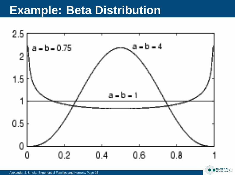
Example: Beta Distribution
Alexander J. Smola: Exponential Families and Kernels, Page 16

Example: Gamma Distribution
Alexander J. Smola: Exponential Families and Kernels, Page 17
UsagePopular as a prior on coefficientsObtained from integral over waiting times in Poissondistribution
Mathematical Form
p(x) = exp(〈(log x, x), (θ1, θ2)〉−log Γ(θ1+1)+(θ1+1) log−θ2)
where the domain is x ∈ [0,∞] and
g(θ) = log Γ(θ1 + 1) + (θ1 + 1) log−θ2)
Note that θ ∈ [0,∞)× (−∞, 0).

Example: Gamma Distribution
Alexander J. Smola: Exponential Families and Kernels, Page 18
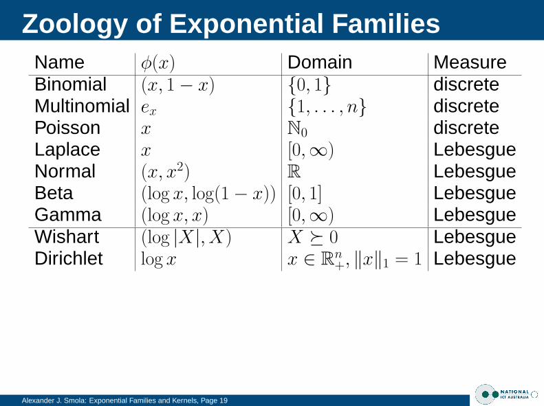
Zoology of Exponential Families
Alexander J. Smola: Exponential Families and Kernels, Page 19
Name φ(x) Domain MeasureBinomial (x, 1− x) {0, 1} discreteMultinomial ex {1, . . . , n} discretePoisson x N0 discreteLaplace x [0,∞) LebesgueNormal (x, x2) R LebesgueBeta (log x, log(1− x)) [0, 1] LebesgueGamma (log x, x) [0,∞) LebesgueWishart (log |X|, X) X � 0 LebesgueDirichlet log x x ∈ Rn
+, ‖x‖1 = 1 Lebesgue

Recall
Alexander J. Smola: Exponential Families and Kernels, Page 20
DefinitionA family of probability distributions which satisfy
p(x; θ) = exp(〈φ(x), θ〉 − g(θ))
Detailsφ(x) is called the sufficient statistics of x.X is the domain out of which x is drawn (x ∈ X).g(θ) is the log-partition function and it ensures that thedistribution integrates out to 1.
g(θ) = log
∫X
exp(〈φ(x), θ〉)dx

Benefits: Log-partition function is nice
Alexander J. Smola: Exponential Families and Kernels, Page 21
g(θ) generates cumulants:
g(θ) = log
∫exp(〈φ(x), θ〉)dx
Taking the derivative wrt. θ we can see that
∂θg(θ) =
∫φ(x) exp(〈φ(x), θ〉)dx∫
exp(〈φ(x), θ〉)dx= Ex∼p(x;θ) [φ(x)]
∂2θg(θ) = Covx∼p(x;θ) [φ(x)]
. . . and so on for higher order cumulants . . .Corollary:
g(θ) is convex

Benefits: Simple Estimation
Alexander J. Smola: Exponential Families and Kernels, Page 22
Likelihood of a set: Given X := {x1, . . . , xm} we get
p(X ; θ) =
m∏i=1
p(xi; θ) = exp
(m∑
i=1
〈φ(xi), θ〉 −mg(θ)
)Maximum Likelihood
We want to minimize the negative log-likelihood, i.e.
minimizeθ
g(θ)−
⟨1
m
m∑i=1
φ(xi), θ
⟩
=⇒ E[φ(x)] =1
m
m∑i=1
φ(xi) =: µ
Solving the maximum likelihood problem is easy .

Application: Laplace distribution
Alexander J. Smola: Exponential Families and Kernels, Page 23
Estimate the decay constant of an atom:We use exponential family notation where
p(x; θ) = exp(〈(−x), θ〉 − (− log θ))
Computing µSince φ(x) = −x all we need to do is average over alldecay times that we observe.
Solving for Maximum LikelihoodThe maximum likelihood condition yields
µ = ∂θg(θ) = ∂θ(− log θ) = −1
θ
This leads to θ = −1µ.

Benefits: Maximum Entropy Estimate
Alexander J. Smola: Exponential Families and Kernels, Page 24
EntropyBasically it’s the number of bits needed to encode a ran-dom variable. It is defined as
H(p) =
∫−p(x) log p(x)dx where we set 0 log 0 := 0
Maximum Entropy DensityThe density p(x) satisfying E[φ(x)] ≥ η with maximumentropy is exp(〈φ(x), θ〉 − g(θ)).
CorollaryThe most vague density with a given variance is theGaussian distribution.
CorollaryThe most vague density with a given mean is the Lapla-cian distribution.

Using it
Alexander J. Smola: Exponential Families and Kernels, Page 25
Observe Datax1, . . . , xm drawn from distribution p(x|θ)
Compute Likelihood
p(X|θ) =
m∏i=1
exp(〈φ(xi), θ〉 − g(θ))
Maximize itTake the negative log and minimize, which leads to
∂θg(θ) =1
m
m∑i=1
φ(xi)
This can be solved analytically or (whenever this is im-possible or we are lazy) by Newton’s method.
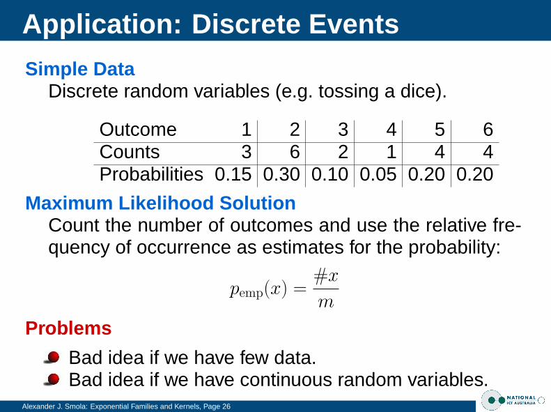
Application: Discrete Events
Alexander J. Smola: Exponential Families and Kernels, Page 26
Simple DataDiscrete random variables (e.g. tossing a dice).
Outcome 1 2 3 4 5 6Counts 3 6 2 1 4 4Probabilities 0.15 0.30 0.10 0.05 0.20 0.20
Maximum Likelihood SolutionCount the number of outcomes and use the relative fre-quency of occurrence as estimates for the probability:
pemp(x) =#x
m
Problems
Bad idea if we have few data.Bad idea if we have continuous random variables.

Tossing a dice
Alexander J. Smola: Exponential Families and Kernels, Page 27

Fisher Information and Efficiency
Alexander J. Smola: Exponential Families and Kernels, Page 28
Fisher ScoreVθ(x) := ∂θ log p(x; θ)
This tells us the influence of x on estimating θ. Its ex-pected value vanishes, since
E [∂θ log p(X ; θ)] =
∫p(X ; θ)∂θ log p(X ; θ)dX
= ∂θ
∫p(X ; θ)dX = 0.
Fisher Information MatrixIt is the covariance matrix of the Fisher scores, that is
I := Cov[Vθ(x)]

Cramer Rao Theorem
Alexander J. Smola: Exponential Families and Kernels, Page 29
EfficiencyCovariance of estimator θ̂(X) rescaled by I:
1/e := det Cov[θ̂(X)]Cov[∂θ log p(X ; θ)]
TheoremThe efficiency for unbiased estimators is never better(i.e. larger) than 1. Equality is achieved for MLEs.
Proof (scalar case only)By Cauchy-Schwartz we have(
Eθ
[(Vθ(X)− Eθ [Vθ(X)])
(θ̂(X)− Eθ
[θ̂(X)
])])2
≤Eθ
[(Vθ(X)− Eθ [Vθ(X)])2
]Eθ
[(θ̂(X)− Eθ
[θ̂(X)
])2]
= IB.

Cramer Rao Theorem
Alexander J. Smola: Exponential Families and Kernels, Page 30
ProofAt the same time, Eθ [Vθ(X)] = 0 implies that
Eθ
[(Vθ(X)− Eθ [Vθ(X)])
(θ̂(X)− Eθ
[θ̂(X)
])]=Eθ
[Vθ(X)θ̂(X)
]=
(∫p(X|θ)∂θ log p(X|θ)θ̂(X)dX
)=∂θ
∫p(X|θ)θ̂(X)dX = ∂θθ = 1.
Cautionary NoteThis does not imply that a biased estimator might nothave lower variance.

Fisher and Exponential Families
Alexander J. Smola: Exponential Families and Kernels, Page 31
Fisher Score
Vθ(x) = ∂θ log p(x; θ)
= φ(x)− ∂θg(θ)
Fisher Information
I = Cov[Vθ(x)]
= Cov[φ(x)− ∂θg(θ)]
= ∂2θg(θ)
Efficiency of estimator can be obtained directly from log-partition function.
Outer Product MatrixIt is given (up to an offset) by 〈φ(x), φ(x′). This leads toKernel-PCA . . .

Priors
Alexander J. Smola: Exponential Families and Kernels, Page 32
Problems with Maximum LikelihoodWith not enough data, parameter estimates will be bad.
Prior to the rescueOften we know where the solution should be. So weencode the latter by means of a prior p(θ).
Normal PriorSimply set p(θ) ∝ exp(− 1
2σ2‖θ‖2).Posterior
p(θ|X) ∝ exp
(m∑
i=1
〈φ(xi), θ〉 − g(θ)− 1
2σ2‖θ‖2
)

Tossing a dice with priors
Alexander J. Smola: Exponential Families and Kernels, Page 33

Conjugate Priors
Alexander J. Smola: Exponential Families and Kernels, Page 34
Problem with Normal PriorThe posterior looks different from the likelihood. Somany of the Maximum Likelihood optimization algorithmsmay not work ...
IdeaWhat if we had a prior which looked like additional data,that is
p(θ|X) ∼ p(X|θ)
For exponential families this is easy. Simply set
p(θ|a) ∝ exp(〈θ, m0a〉 −m0g(θ))
Posterior
p(θ|X) ∝ exp
((m + m0)
(⟨mµ + m0a
m + m0, θ
⟩− g(θ)
))

Example: Multinomial Distribution
Alexander J. Smola: Exponential Families and Kernels, Page 35
Laplace RuleA conjugate prior with parameters (a, m0) in the multino-mial family could be to set a = (1
n,1n, . . . ,
1n). This is often
also called the Dirichlet prior . It leads to
p(x) =#x + m0/n
m + m0instead of p(x) =
#x
m
ExampleOutcome 1 2 3 4 5 6Counts 3 6 2 1 4 4MLE 0.15 0.30 0.10 0.05 0.20 0.20MAP (m0 = 6) 0.25 0.27 0.12 0.08 0.19 0.19MAP (m0 = 100) 0.16 0.19 0.16 0.15 0.17 0.17

Optimization Problems
Alexander J. Smola: Exponential Families and Kernels, Page 36
Maximum Likelihood
minimizeθ
m∑i=1
g(θ)− 〈φ(xi), θ〉 =⇒ ∂θg(θ) =1
m
m∑i=1
φ(xi)
Normal Prior
minimizeθ
m∑i=1
g(θ)− 〈φ(xi), θ〉 +1
2σ2‖θ‖2
Conjugate Prior
minimizeθ
m∑i=1
g(θ)− 〈φ(xi), θ〉 + m0g(θ)−m0〈µ̃, θ〉
equivalently solve ∂θg(θ) =1
m + m0
m∑i=1
φ(xi) +m0
m + m0µ̃

Summary
Alexander J. Smola: Exponential Families and Kernels, Page 37
ModelLog partition functionExpectations and derivativesMaximum entropy formulation
A Zoo of DensitiesEstimation
Maximum Likelihood EstimatorFisher Information Matrix and Cramer Rao TheoremNormal Priors and Conjugate PriorsFisher information and log-partition function

Alexander J. Smola: Exponential Families and Kernels, Page 1
Exponential Families and KernelsLecture 2
Alexander J. [email protected]
Machine Learning ProgramNational ICT Australia
RSISE, The Australian National University

Outline
Alexander J. Smola: Exponential Families and Kernels, Page 2
Exponential FamiliesMaximum likelihood and Fisher informationPriors (conjugate and normal)
Conditioning and Feature SpacesConditional distributions and inner productsClifford Hammersley Decomposition
ApplicationsClassification and novelty detectionRegression
ApplicationsConditional random fieldsIntractable models and semidefinite approximations

Lecture 2
Alexander J. Smola: Exponential Families and Kernels, Page 3
Clifford Hammersley Theorem and Graphical ModelsDecomposition resultsKey connection
Conditional DistributionsLog partition functionExpectations and derivativesInner product formulation and kernelsGaussian Processes
ApplicationsClassification + RegressionConditional Random FieldsSpatial Poisson Models

Graphical Model
Alexander J. Smola: Exponential Families and Kernels, Page 4
Conditional Independencex, x′ are conditionally independent given c, if
p(x, x′|c) = p(x|c)p(x′|c)Distributions can be simplified greatly by conditionalindependence assumptions.
Markov NetworkGiven a graph G(V,E) with vertices V and edges Eassociate a random variable x ∈ R|V | with G.Subsets of random variables xS, xS′ are conditionallyindependent given xC if removing the vertices C fromG(V,E) decomposes the graph into disjoint subsetscontaining S, S ′.

Conditional Independence
Alexander J. Smola: Exponential Families and Kernels, Page 5
Cliques
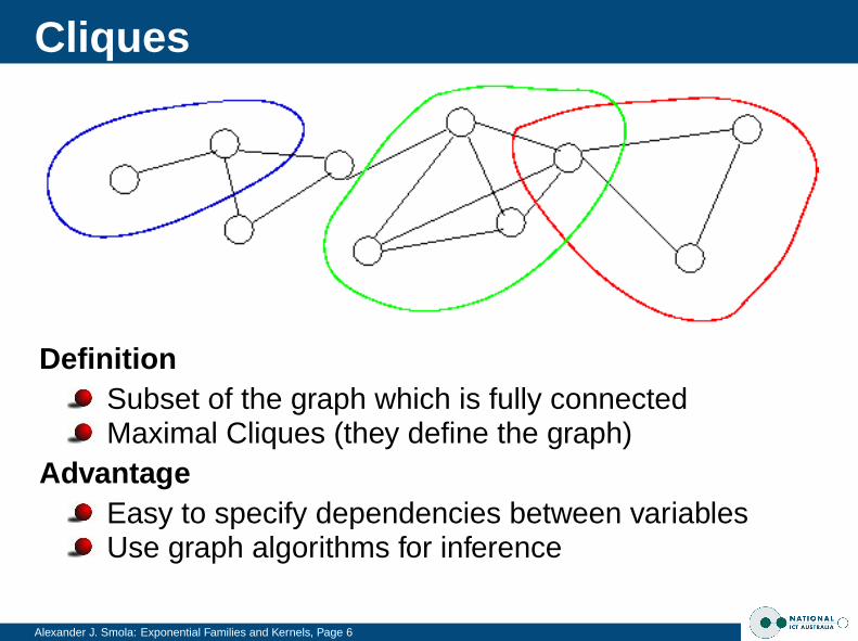
Alexander J. Smola: Exponential Families and Kernels, Page 6
DefinitionSubset of the graph which is fully connectedMaximal Cliques (they define the graph)
AdvantageEasy to specify dependencies between variablesUse graph algorithms for inference
Hammersley Clifford Theorem
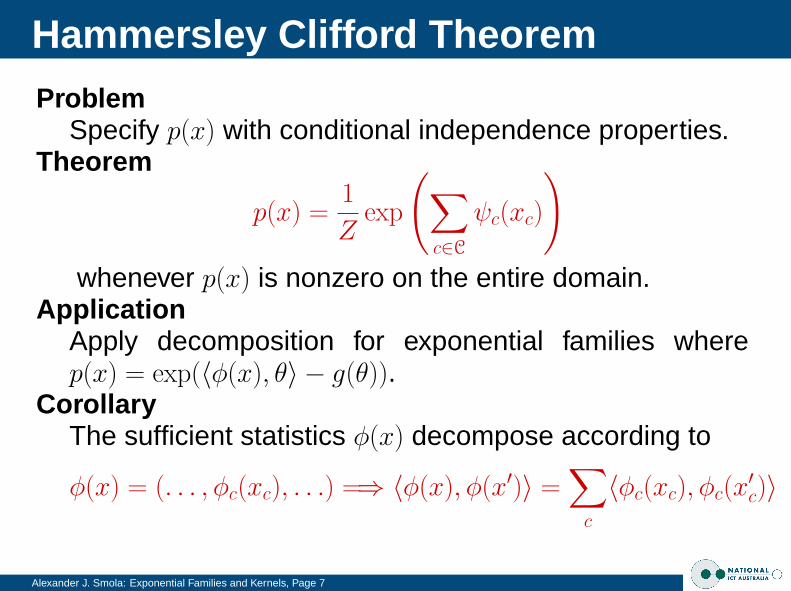
Alexander J. Smola: Exponential Families and Kernels, Page 7
ProblemSpecify p(x) with conditional independence properties.
Theorem
p(x) =1
Zexp
(∑c∈C
ψc(xc)
)whenever p(x) is nonzero on the entire domain.
ApplicationApply decomposition for exponential families wherep(x) = exp(〈φ(x), θ〉 − g(θ)).
CorollaryThe sufficient statistics φ(x) decompose according to
φ(x) = (. . . , φc(xc), . . .) =⇒ 〈φ(x), φ(x′)〉 =∑c
〈φc(xc), φc(x′c)〉

Proof
Alexander J. Smola: Exponential Families and Kernels, Page 8
Step 1: Obtain linear functionalCombing the exponential setting with the CH theorem:
〈Φ(x), θ〉 =∑c∈C
ψc(xc)− logZ + g(θ) for all x, θ.
Step 2: Orthonormal basis in θPick an orthonormal basis and swallow Z, g. This gives
〈Φ(x), ei〉 =∑c∈C
ηic(xc) for some ηic(xc).
Step 3: Reconstruct sufficient statistics
Φc(xc) := (η1c (xc), η
2c (xc), . . .)
which allows us to compute
〈Φ(x), θ〉 =∑c∈C
∑i
θiΦic(xc).

Example: Normal Distributions
Alexander J. Smola: Exponential Families and Kernels, Page 9
Sufficient StatisticsRecall that for normal distributions φ(x) = (x, xx>).
Clifford Hammersley Applicationφ(x) must decompose into subsets involving only vari-ables from each maximal clique.The linear term x is OK by default.The only nonzero terms coupling xixj are those corre-sponding to an edge in the graph G(V,E).
Inverse Covariance MatrixThe natural parameter aligned with xx> is the inversecovariance matrix.Its sparsity mirrors G(V,E).Hence a sparse inverse kernel matrix corresponds tographical model!

Example: Normal Distributions
Alexander J. Smola: Exponential Families and Kernels, Page 10
Density
p(x|θ) = exp
n∑i=1
xiθ1i +
n∑i,j=1
xixjθ2ij − g(θ)
Here θ2 = Σ−1, is the inverse covariance matrix. We havethat (Σ−1)[ij] 6= 0 only if (i, j) share an edge.
Conditional Distributions
Alexander J. Smola: Exponential Families and Kernels, Page 11
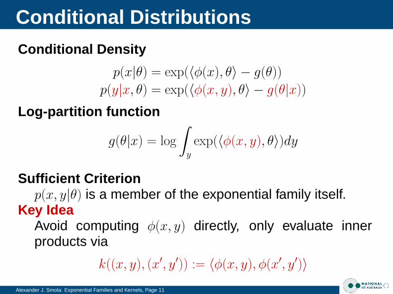
Conditional Density
p(x|θ) = exp(〈φ(x), θ〉 − g(θ))
p(y|x, θ) = exp(〈φ(x, y), θ〉 − g(θ|x))
Log-partition function
g(θ|x) = log
∫y
exp(〈φ(x, y), θ〉)dy
Sufficient Criterionp(x, y|θ) is a member of the exponential family itself.
Key IdeaAvoid computing φ(x, y) directly, only evaluate innerproducts via
k((x, y), (x′, y′)) := 〈φ(x, y), φ(x′, y′)〉

Conditional Distributions
Alexander J. Smola: Exponential Families and Kernels, Page 12
Maximum a Posteriori Estimation
− log p(θ|X) =
m∑i=1
−〈φ(xi), θ〉 +mg(θ) +1
2σ2‖θ‖2 + c
− log p(θ|X, Y ) =
m∑i=1
−〈φ(xi, yi), θ〉 + g(θ|xi) +1
2σ2‖θ‖2 + c
Solving the ProblemThe problem is strictly convex in θ.Direct solution is impossible if we cannot computeφ(x, y) directly.Solve convex problem in expansion coefficients.Expand θ in a linear combination of φ(xi, y).

Joint Feature Map
Alexander J. Smola: Exponential Families and Kernels, Page 13

Representer Theorem
Alexander J. Smola: Exponential Families and Kernels, Page 14
Objective Function
− log p(θ|X, Y ) =
m∑i=1
−〈φ(xi, yi), θ〉 + g(θ|xi) +1
2σ2‖θ‖2 + c
DecompositionDecompose θ into θ = θ‖ + θ⊥ where
θ‖ ∈ span{φ(xi, y) where 1 ≤ i ≤ m and y ∈ Y}Both g(θ|xi)and 〈φ(xi, yi), θ〉are independent of θ⊥.
Theorem− log p(θ|X, Y ) is minimized for θ⊥ = 0, hence θ = θ‖.
ConsequenceIf span{φ(xi, y) where 1 ≤ i ≤ m and y ∈ Y} is finite di-mensional, we have a parametric optimization problem.
Using It
Alexander J. Smola: Exponential Families and Kernels, Page 15
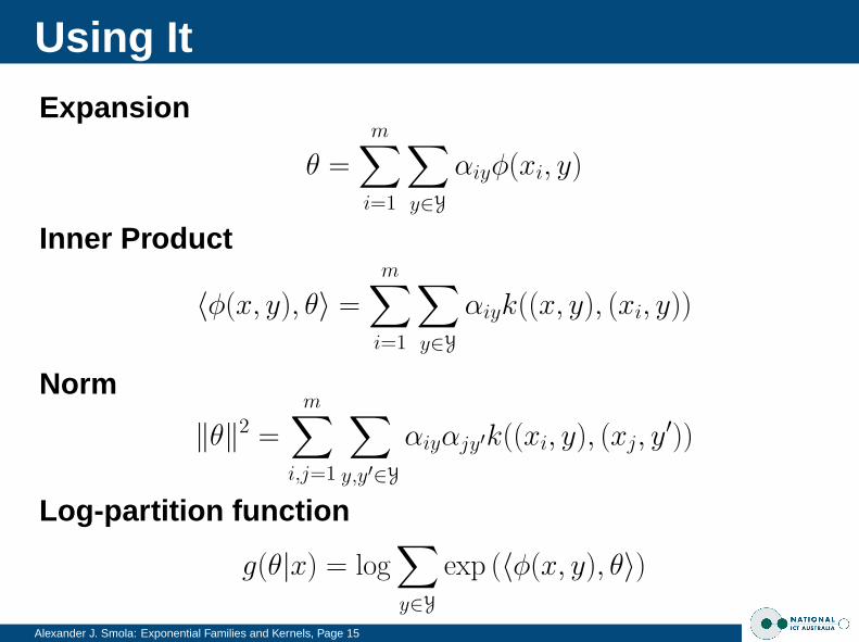
Expansion
θ =
m∑i=1
∑y∈Y
αiyφ(xi, y)
Inner Product
〈φ(x, y), θ〉 =
m∑i=1
∑y∈Y
αiyk((x, y), (xi, y))
Norm
‖θ‖2 =
m∑i,j=1
∑y,y′∈Y
αiyαjy′k((xi, y), (xj, y′))
Log-partition function
g(θ|x) = log∑y∈Y
exp (〈φ(x, y), θ〉)

The Gaussian Process Link
Alexander J. Smola: Exponential Families and Kernels, Page 16
Normal Prior on θ . . .
θ ∼ N(0, σ21)
. . . yields Normal Prior on t(x, y) = 〈φ(x, y), θ〉Distribution of projected Gaussian is Gaussian.The mean vanishes
Eθ[t(x, y)] = 〈φ(x, y),Eθ[θ]〉 = 0
The covariance yields
Cov[t(x, y), t(x′, y′)] = Eθ [〈φ(x, y), θ〉〈θ, φ(x′, y′)〉]= σ2〈φ(x, y), φ(x′, y′)〉︸ ︷︷ ︸
:=k((x,y),(x′,y′))
. . . so we have a Gaussian Process on x . . .with kernel k((x, y), (x′, y′)) = σ2〈φ(x, y), φ(x′, y′)〉.

Linear Covariance
Alexander J. Smola: Exponential Families and Kernels, Page 17
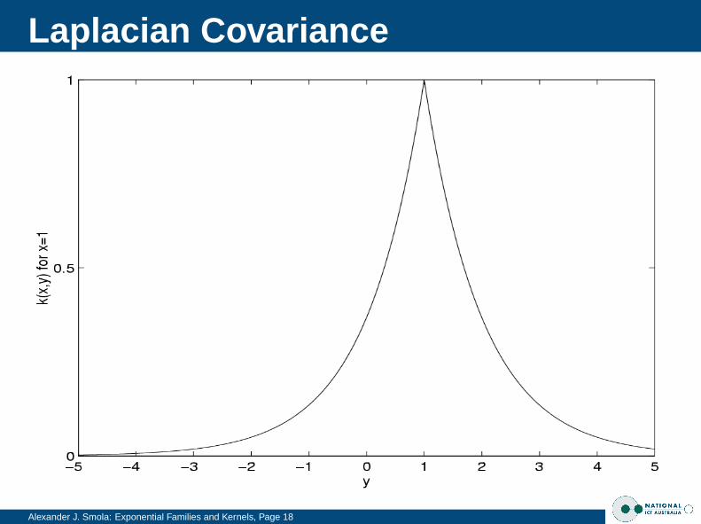
Laplacian Covariance
Alexander J. Smola: Exponential Families and Kernels, Page 18

Gaussian Covariance
Alexander J. Smola: Exponential Families and Kernels, Page 19
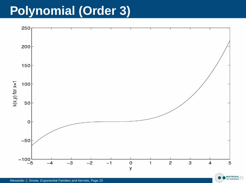
Polynomial (Order 3)
Alexander J. Smola: Exponential Families and Kernels, Page 20

B3-Spline Covariance
Alexander J. Smola: Exponential Families and Kernels, Page 21
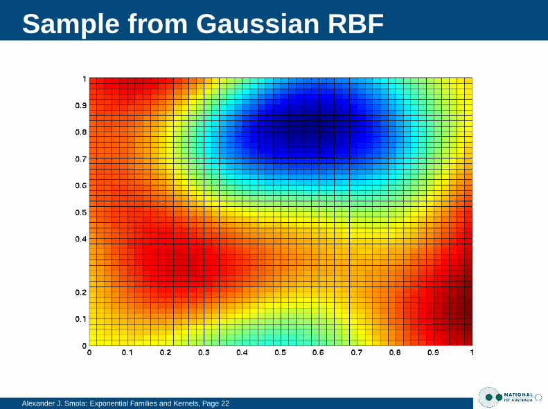
Sample from Gaussian RBF
Alexander J. Smola: Exponential Families and Kernels, Page 22

Sample from Gaussian RBF
Alexander J. Smola: Exponential Families and Kernels, Page 23

Sample from Gaussian RBF
Alexander J. Smola: Exponential Families and Kernels, Page 24
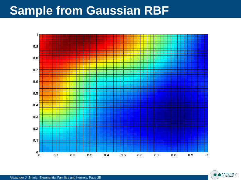
Sample from Gaussian RBF
Alexander J. Smola: Exponential Families and Kernels, Page 25

Sample from Gaussian RBF
Alexander J. Smola: Exponential Families and Kernels, Page 26

Sample from linear kernel
Alexander J. Smola: Exponential Families and Kernels, Page 27

Sample from linear kernel
Alexander J. Smola: Exponential Families and Kernels, Page 28

Sample from linear kernel
Alexander J. Smola: Exponential Families and Kernels, Page 29

Sample from linear kernel
Alexander J. Smola: Exponential Families and Kernels, Page 30

Sample from linear kernel
Alexander J. Smola: Exponential Families and Kernels, Page 31

General Strategy
Alexander J. Smola: Exponential Families and Kernels, Page 32
Choose a suitable sufficient statistic φ(x, y)
Conditionally multinomial distribution leads to Gaus-sian Process multiclass estimator: we have a distribu-tion over n classes which depends on x.Conditionally Gaussian leads to Gaussian Process re-gression: we have a normal distribution over a randomvariable which depends on the location.Note: we estimate mean and variance.Conditionally Poisson distributions yield locally vary-ing Poisson processes. This has no name yet ...
Solve the optimization problemThis is typically convex.
The bottom lineInstead of choosing k(x, x′) choose k((x, y), (x′, y′)).
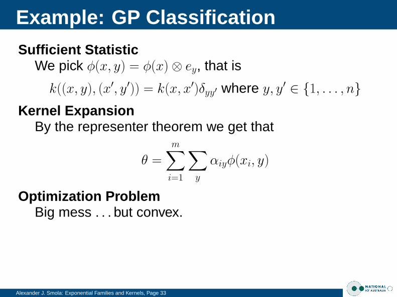
Example: GP Classification
Alexander J. Smola: Exponential Families and Kernels, Page 33
Sufficient StatisticWe pick φ(x, y) = φ(x)⊗ ey, that is
k((x, y), (x′, y′)) = k(x, x′)δyy′ where y, y′ ∈ {1, . . . , n}Kernel Expansion
By the representer theorem we get that
θ =
m∑i=1
∑y
αiyφ(xi, y)
Optimization ProblemBig mess . . . but convex.
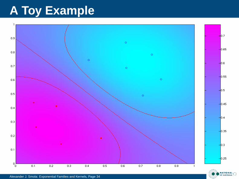
A Toy Example
Alexander J. Smola: Exponential Families and Kernels, Page 34

Noisy Data
Alexander J. Smola: Exponential Families and Kernels, Page 35
Summary
Alexander J. Smola: Exponential Families and Kernels, Page 36
Clifford Hammersley Theorem and Graphical ModelsDecomposition resultsKey connectionNormal distribution
Conditional DistributionsLog partition functionExpectations and derivativesInner product formulation and kernelsGaussian Processes
ApplicationsGeneralized kernel trickConditioning gives existing estimation methods back

Alexander J. Smola: Exponential Families and Kernels, Page 1
Exponential Families and KernelsLecture 3
Alexander J. [email protected]
Machine Learning ProgramNational ICT Australia
RSISE, The Australian National University

Outline
Alexander J. Smola: Exponential Families and Kernels, Page 2
Exponential FamiliesMaximum likelihood and Fisher informationPriors (conjugate and normal)
Conditioning and Feature SpacesConditional distributions and inner productsClifford Hammersley Decomposition
ApplicationsClassification and novelty detectionRegression
ApplicationsConditional random fieldsIntractable models and semidefinite approximations

Lecture 3
Alexander J. Smola: Exponential Families and Kernels, Page 3
Novelty DetectionDensity estimationThresholding and likelihood ratio
ClassificationLog partition functionOptimization problemExamplesClustering and transduction
RegressionConditional normal distributionEstimating the covarianceHeteroscedastic estimators

Density Estimation
Alexander J. Smola: Exponential Families and Kernels, Page 4
Maximum a Posteriori
minimizeθ
m∑i=1
g(θ)− 〈φ(xi), θ〉 +1
2σ2‖θ‖2
AdvantagesConvex optimization problemConcentration of measure
ProblemsNormalization g(θ) may be painful to computeFor density estimation we need no normalized p(x|θ)No need to perform particularly well in high densityregions
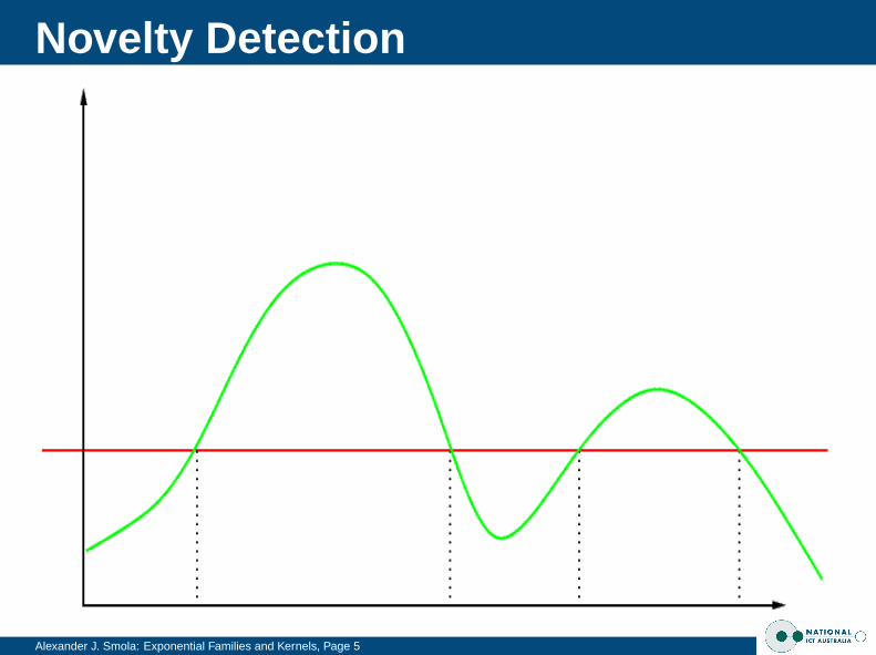
Novelty Detection
Alexander J. Smola: Exponential Families and Kernels, Page 5

Novelty Detection
Alexander J. Smola: Exponential Families and Kernels, Page 6
Optimization Problem
MAPm∑
i=1
− log p(xi|θ) +1
2σ2‖θ‖2
Noveltym∑
i=1
max
(− log
p(xi|θ)
exp(ρ− g(θ)), 0
)+
1
2‖θ‖2
m∑i=1
max(ρ− 〈φ(xi), θ〉, 0) +1
2‖θ‖2
AdvantagesNo normalization g(θ) neededNo need to perform particularly well in high densityregions (estimator focuses on low-density regions)Quadratic program

Geometric Interpretation
Alexander J. Smola: Exponential Families and Kernels, Page 7
IdeaFind hyperplane that has maximum distance from ori-gin , yet is still closer to the origin than the observations.
Hard Margin
minimize1
2‖θ‖2
subject to 〈θ, xi〉 ≥ 1
Soft Margin
minimize1
2‖θ‖2 + C
m∑i=1
ξi
subject to 〈θ, xi〉 ≥ 1− ξi
ξi ≥ 0
Dual Optimization Problem
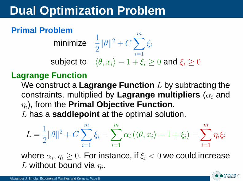
Alexander J. Smola: Exponential Families and Kernels, Page 8
Primal Problem
minimize1
2‖θ‖2 + C
m∑i=1
ξi
subject to 〈θ, xi〉 − 1 + ξi ≥ 0 and ξi ≥ 0
Lagrange FunctionWe construct a Lagrange Function L by subtracting theconstraints, multiplied by Lagrange multipliers (αi andηi), from the Primal Objective Function .L has a saddlepoint at the optimal solution.
L =1
2‖θ‖2 + C
m∑i=1
ξi −m∑
i=1
αi (〈θ, xi〉 − 1 + ξi)−m∑
i=1
ηiξi
where αi, ηi ≥ 0. For instance, if ξi < 0 we could increaseL without bound via ηi.

Dual Problem, Part II
Alexander J. Smola: Exponential Families and Kernels, Page 9
Optimality Conditions
∂θL = θ −m∑
i=1
αixi = 0 =⇒ θ =
m∑i=1
αixi
∂ξiL = C − αi − ηi = 0 =⇒ αi ∈ [0, C]
Now we substitute the two optimality conditions backinto L and eliminate the primal variables .
Dual Problem
minimize1
2
m∑i=1
αiαj〈xi, xj〉 −m∑
i=1
αi
subject to αi ∈ [0, C]
Convexity ensures uniqueness of the optimum.

The ν-Trick
Alexander J. Smola: Exponential Families and Kernels, Page 10
ProblemDepending on how we choose C, the number of pointsselected as lying on the “wrong” side of the hyperplaneH := {x|〈θ, x〉 = 1} will vary.
We would like to specify a certain fraction ν before-hand.We want to make the setting more adaptive to thedata.
SolutionUse adaptive hyperplane that separates data from theorigin, i.e. find
H := {x|〈θ, x〉 = ρ},where the threshold ρ is adaptive .

The ν-Trick
Alexander J. Smola: Exponential Families and Kernels, Page 11
Primal Problem
minimize1
2‖θ‖2 +
m∑i=1
ξi −mνρ
subject to 〈θ, xi〉 − ρ + ξi ≥ 0 and ξi ≥ 0
Dual Problem
minimize1
2
m∑i=1
αiαj〈xi, xj〉
subject to αi ∈ [0, 1] andm∑
i=1
αi = νm.
Difference to beforeThe
∑i αi term vanishes from the objective function but
we get one more constraint, namely∑
i αi = νm.

The ν-Property
Alexander J. Smola: Exponential Families and Kernels, Page 12
Optimization Problem
minimize1
2‖θ‖2 +
m∑i=1
ξi −mνρ
subject to 〈θ, xi〉 − ρ + ξi ≥ 0 and ξi ≥ 0
TheoremAt most a fraction of ν points will lie on the “wrong”side of the margin, i.e., yif (xi) < 1.At most a fraction of 1 − ν points will lie on the “right”side of the margin, i.e., yif (xi) > 1.In the limit, those fractions will become exact.
Proof IdeaAt optimum, shift ρ slightly: only the active constraintswill have an influence on the objective function.

Classification
Alexander J. Smola: Exponential Families and Kernels, Page 13
Maximum a Posteriori Estimation
− log p(θ|X, Y ) =
m∑i=1
−〈φ(xi, yi), θ〉 + g(θ|xi) +1
2σ2‖θ‖2 + c
DomainFinite set of observations Y = {1, . . . ,m}Log-partition function g(θ|x) easy to compute.Optional centering
φ(x, y) → φ(x, y) + c
leaves p(y|x, θ) unchanged (offsets both terms).Gaussian Process Connection
Inner product t(x, y) = 〈φ(x, y), θ〉 is drawn from Gaus-sian process, so same setting as in literature.

Classification
Alexander J. Smola: Exponential Families and Kernels, Page 14
Sufficient StatisticWe pick φ(x, y) = φ(x)⊗ ey, that is
k((x, y), (x′, y′)) = k(x, x′)δyy′ where y, y′ ∈ {1, . . . , n}Kernel Expansion
By the representer theorem we get that
θ =
m∑i=1
∑y
αiyφ(xi, y)
Optimization ProblemBig mess . . . but convex.Solve by Newton or Block-Jacobi method.

A Toy Example
Alexander J. Smola: Exponential Families and Kernels, Page 15

Noisy Data
Alexander J. Smola: Exponential Families and Kernels, Page 16

SVM Connection
Alexander J. Smola: Exponential Families and Kernels, Page 17
Problems with GP ClassificationOptimize even where classification is goodOnly sign of classification neededOnly “strongest” wrong class mattersWant to classify with a margin
Optimization Problem
MAPm∑
i=1
− log p(yi|xi, θ) +1
2σ2‖θ‖2
SVMm∑
i=1
max
(ρ− log
p(yi|xi, θ)
maxy 6=yip(y|xi, θ)
, 0
)+
1
2‖θ‖2
m∑i=1
max(ρ− 〈φ(xi, yi), θ〉 + maxy 6=yi
〈φ(xi, y), θ〉, 0) +1
2‖θ‖2

Binary Classification
Alexander J. Smola: Exponential Families and Kernels, Page 18
Sufficient StatisticsOffset in φ(x, y) can be arbitraryPick such that φ(x, y) = yφ(x)where y ∈ {±1}.Kernel matrix becomes
Kij = k((xi, yi), (xj, yj)) = yiyjk(xi, xj)
Optimization ProblemThe max over other classes becomes
maxy 6=yi
〈φ(xi, y), θ〉 = −y〈φ(xi), θ〉
Overall problemm∑
i=1
max(ρ− 2yi〈φ(xi), θ〉, 0) +1
2‖θ‖2

Geometrical Interpretation
Alexander J. Smola: Exponential Families and Kernels, Page 19
Minimize1
2‖θ‖2 subject to yi(〈θ, xi〉 + b) ≥ 1 for all i.

Optimization Problem
Alexander J. Smola: Exponential Families and Kernels, Page 20
Linear Functionf (x) = 〈θ, x〉 + b
Mathematical Programming SettingIf we require error-free classification with a margin, i.e.,yf (x) ≥ 1, we obtain:
minimize1
2‖θ‖2
subject to yi(〈θ, xi〉 + b)− 1 ≥ 0 for all 1 ≤ i ≤ m
ResultThe dual of the optimization problem is a simplequadratic program (more later ...).
Connection back to conditional probabilitiesOffset b takes care of bias towards one of the classes.

Regression
Alexander J. Smola: Exponential Families and Kernels, Page 21
Maximum a Posteriori Estimation
− log p(θ|X, Y ) =
m∑i=1
−〈φ(xi, yi), θ〉 + g(θ|xi) +1
2σ2‖θ‖2 + c
DomainContinuous domain of observations Y = RLog-partition function g(θ|x) easy to compute inclosed form as normal distribution.
Gaussian Process ConnectionInner product t(x, y) = 〈φ(x, y), θ is drawn from Gaussianprocess. In particular also rescaled mean and covari-ance.

Regression
Alexander J. Smola: Exponential Families and Kernels, Page 22
Sufficient Statistic (Standard Model)We pick φ(x, y) = (yφ(x), y2), that is
k((x, y), (x′, y′)) = k(x, x′)yy′ + y2y′2 where y, y′ ∈ R
Traditionally the variance is fixed, that is θ2 = const..Sufficient Statistic (Fancy Model)
We pick φ(x, y) = (yφ1(x), y2φ2(x)), that is
k((x, y), (x′, y′)) = k1(x, x′)yy′+k2(x, x′)y2y′2 where y, y′ ∈ R
We estimate mean and variance simultaneously .Kernel Expansion
By the representer theorem (and more algebra) we get
θ =
(m∑
i=1
αi1φ1(xi),
m∑i=1
αi2φ2(xi)
)

Training Data
Alexander J. Smola: Exponential Families and Kernels, Page 23

Mean ~k>(x)(K + σ21)−1y
Alexander J. Smola: Exponential Families and Kernels, Page 24

Variance k(x, x) + σ2 − ~k>(x)(K + σ21)−1~k(x)
Alexander J. Smola: Exponential Families and Kernels, Page 25

Putting everything together . . .
Alexander J. Smola: Exponential Families and Kernels, Page 26

Another Example
Alexander J. Smola: Exponential Families and Kernels, Page 27

Adaptive Variance Method
Alexander J. Smola: Exponential Families and Kernels, Page 28
Optimization Problem:
minimizem∑
i=1
−14
m∑j=1
α1jk1(xi, xj)
> m∑j=1
α2jk2(xi, xj)
−1 m∑j=1
α1jk1(xi, xj)
−1
2log det−2
m∑j=1
α2jk2(xi, xj)
− m∑j=1
[y>i α1jk1(xi, xj) + (y>j α2jyj)k2(xi, xj)
]+
12σ2
∑i,j
α>1iα1jk1(xi, xj) + tr[α2iα
>2j
]k2(xi, xj).
subject to 0 �m∑
i=1
α2ik(xi, xj)
Properties of the problem:The problem is convexThe log-determinant from the normalization of theGaussian acts as a barrrier function .We get a semidefinite program.

Heteroscedastic Regression
Alexander J. Smola: Exponential Families and Kernels, Page 29

Natural Parameters
Alexander J. Smola: Exponential Families and Kernels, Page 30

Lecture 3
Alexander J. Smola: Exponential Families and Kernels, Page 31
Novelty DetectionDensity estimationThresholding and likelihood ratio
ClassificationLog partition functionOptimization problemExamplesClustering and transduction
RegressionConditional normal distributionEstimating the covarianceHeteroscedastic estimators

Alexander J. Smola: Exponential Families and Kernels, Page 1
Exponential Families and KernelsLecture 4
Alexander J. [email protected]
Machine Learning ProgramNational ICT Australia
RSISE, The Australian National University

Outline
Alexander J. Smola: Exponential Families and Kernels, Page 2
Exponential FamiliesMaximum likelihood and Fisher informationPriors (conjugate and normal)
Conditioning and Feature SpacesConditional distributions and inner productsClifford Hammersley Decomposition
ApplicationsClassification and novelty detectionRegression
ApplicationsConditional random fieldsIntractable models and semidefinite approximations

Lecture 4
Alexander J. Smola: Exponential Families and Kernels, Page 3
Conditional Random FieldsStructured random variablesSubspace representer theorem and decompositionDerivatives and conditional expectations
Inference and Message PassingDynamic programmingMessage passing and junction treesIntractable cases
Semidefinite RelaxationsMarginal polytopesFenchel duality and entropyRelaxations for conditional random fields

Hammersley Clifford Corollary
Alexander J. Smola: Exponential Families and Kernels, Page 4
DecompositionThe sufficient statistics φ(x) decompose according to
φ(x) = (. . . , φc(xc), . . .)
Consequently we can write the kernel via
k(x, x′) = 〈φ(x), φ(x′)〉 =∑
c
〈φc(xc), φc(x′c)〉 =
∑c
kc(xc, x′c)

Conditional Random Fields
Alexander J. Smola: Exponential Families and Kernels, Page 5
Key PointsCliques are (xt, yt), (xt, xt+1), and (yt, yt+1)We can drop cliques in (xt, xt+1): they do not affectp(y|x, θ):
p(y|x, θ) = exp( ∑
t
〈φxy(xt, yt), θxy,t〉 + 〈φyy(yt, yt+1), θyy,t〉+
〈φxx(xt, xt+1), θxx,t〉 − g(θ|x))

Computational Issues
Alexander J. Smola: Exponential Families and Kernels, Page 6
Key PointsCompute g(θ|x) via dynamicAssume stationarity of the model, that is θc does notdepend on the position of the
Dynamic Programming
g(θ|x)
= log∑
y1,...,yT
T∏t=1
exp (〈φxy(xt, yt), θxy〉 + 〈φyy(yt, yt+1), θyy〉)︸ ︷︷ ︸Mt(yt,yt+1)
= log∑y1
∑y2
M1(y1, y2)∑y3
M2(y2, y3) . . .∑yT
MT (yT−1, yT )
So we can compute g(θ|x), p(yt|x, θ) and p(yt, yt+1|x, θ)via dynamic programming.

Forward Backward Algorithm
Alexander J. Smola: Exponential Families and Kernels, Page 7
Key IdeaStore sum over all y1, . . . , yt−1 (forward pass) and overall yt+1, . . . , yT as intermediate valuesWe get those values for all positions t in one sweep.Extend this to message passing (when we have trees).

Minimization
Alexander J. Smola: Exponential Families and Kernels, Page 8
Objective Function
− log p(θ|X,Y ) =
m∑i=1
−〈φ(xi, yi), θ〉 + g(θ|xi) +1
2σ2‖θ‖2 + c
∂θ − log p(θ|X,Y ) =
m∑i=1
−φ(xi, yi) + E [φ(xi, yi)|xi] +1
σ2θ
We only need E [φxy(xit, yit)|xi] and E[φyy(yit, yi(t+1))|xi
].
Kernel TrickConditional expectations of Φ(xit, yit) cannot be com-puted explicitly but inner products can.
〈φxy(x′t, y
′t),E [φxy(xt, yt)|x] = E [k((x′
t, y′t), (xt, yt)|x]
Only need marginals p(yt|x, θ) and p(yt, yt+1|x, θ),which we get via dynamic programming.

Subspace Representer Theorem
Alexander J. Smola: Exponential Families and Kernels, Page 9
Representer TheoremSolutions of the MAP problem are given by
θ ∈ span{φ(xi, y) for all y ∈ Y and 1 ≤ i ≤ n}Big Problem
|Y| could be huge, e.g. for sequence annotation 2n.Solution
Exploit decomposition of φ(x, y) into sufficient statis-tics on cliques.Restriction of Y to cliques is much smaller.
θc ∈ span{φc(xci, yc) for all yc ∈ Yc and 1 ≤ i ≤ n}Rather than 2n we now get 2|c|.
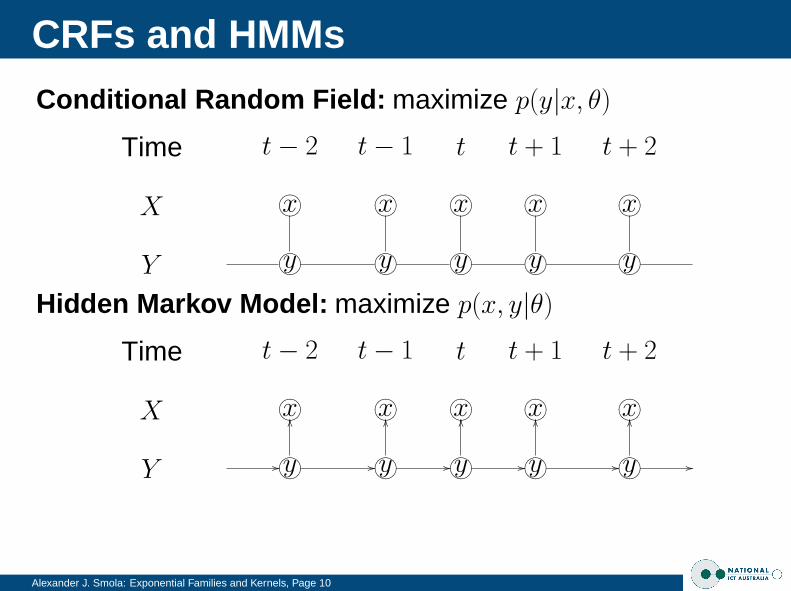
CRFs and HMMs
Alexander J. Smola: Exponential Families and Kernels, Page 10
Conditional Random Field: maximize p(y|x, θ)
Time t − 2 t − 1 t t + 1 t + 2
X ?>=<89:;x ?>=<89:;x ?>=<89:;x ?>=<89:;x ?>=<89:;x
Y ?>=<89:;y ?>=<89:;y ?>=<89:;y ?>=<89:;y ?>=<89:;y
Hidden Markov Model: maximize p(x, y|θ)
Time t − 2 t − 1 t t + 1 t + 2
X ?>=<89:;x ?>=<89:;x ?>=<89:;x ?>=<89:;x ?>=<89:;x
Y //?>=<89:;y //
OO
?>=<89:;y //
OO
?>=<89:;y //
OO
?>=<89:;y //
OO
?>=<89:;y //
OO

Equivalence Theorem
Alexander J. Smola: Exponential Families and Kernels, Page 11
TheoremCRFs and HMMs yield identical probability estimates forp(y|x, θ), if the set of functions is equally expressive.
ProofWrite out pCRF(y|x, θ) and pHMM(x, y|θ), and show thatthey only differ in the normalization.This disappears when computing pHMM(y|x, θ).
ConsequenceDifferential training for current HMM implementations.

Message Passing
Alexander J. Smola: Exponential Families and Kernels, Page 12
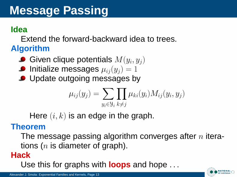
Message Passing
Alexander J. Smola: Exponential Families and Kernels, Page 13
IdeaExtend the forward-backward idea to trees.
AlgorithmGiven clique potentials M(yi, yj)Initialize messages µij(yj) = 1Update outgoing messages by
µij(yj) =∑yi∈Yi
∏k 6=j
µki(yi)Mij(yi, yj)
Here (i, k) is an edge in the graph.Theorem
The message passing algorithm converges after n itera-tions (n is diameter of graph).
HackUse this for graphs with loops and hope . . .

Junction Trees
Alexander J. Smola: Exponential Families and Kernels, Page 14
Stock standard algorithms available to transform graph intojunction tree. Now we can use message passing . . .

Junction Tree Algorithm
Alexander J. Smola: Exponential Families and Kernels, Page 15
IdeaMessages involve variables in the separator sets.
AlgorithmGiven clique potentials Mc(yc) and separator sets s.Initialize messages µc,s(ys) = 1Update outgoing messages by
µc,s(ys) =∑yc\ys
∏s′ 6=s
µc′,s′(ys′)Mc(yc)
Here s′ is a separator set connecting c with c′.Theorem
The message passing algorithm converges after n itera-tions (n is diameter of the hypergraph).
HackUse this for graphs with loops and hope . . .

Example
Alexander J. Smola: Exponential Families and Kernels, Page 16

Problems
Alexander J. Smola: Exponential Families and Kernels, Page 17
ScalingThe algorithm scales exponentially in the treewidth.Messages are of size d|Ys|.
Convergence with loopsUse of message passing may or may not converge. Noreal proof available.
WorkaroundUse a subset of the graph and solve the inference prob-lem with this. Average over spanning trees.
WorkaroundUse sampling methods for inference.

A Better Way
Alexander J. Smola: Exponential Families and Kernels, Page 18
Fenchel DualityCompute dual of log-partition function via
g∗(µ) = supθ∈Θ
〈µ, θ〉 − g(θ) (Θ is a convex domain)
Entropy and Expectation ParametersThe maximum of the optimization problem is obtained forµ = ∂θg(θ). This leads to
H =
∫− log p(x|θ)p(x|θ)dθ = −〈µ(θ), θ〉 + g(θ) = −g∗(µ)
Strong DualityDualizing again leads to
g(θ) = supµ∈M
〈θ, µ〉 + H(µ)

Semidefinite Relaxation
Alexander J. Smola: Exponential Families and Kernels, Page 19
Optimization Problem
g(θ) = supµ∈M
〈θ, µ〉 + H(µ)
Here M is the set of all possible marginals.Relaxations on M
The polytope M is convex (by duality), however it is hardto compute (as hard as g(θ)). So we relax it to M̃ byimpose constraints on higher order moments, such as
Interval and linear inequality constraints.SDP constraints on the covariance matrix.
Upper bound on H(µ)Gaussian bound on the covariance via G(µ). So we get
g(θ) ≤ supµ∈M̃
〈θ, µ〉 + G(µ)

Application to CRFs
Alexander J. Smola: Exponential Families and Kernels, Page 20
Optimization Problem
− log p(θ|X,Y )
=
m∑i=1
−〈φ(xi, yi), θ〉 + g(θ|xi) +1
2σ2‖θ‖2 + c
≤m∑
i=1
supµi∈M̃i
〈θ, µi − φ(xi, yi)〉 + H(µi) +1
2σ2‖θ‖2
Technical DetailsMinimization over θ and µi can be swapped (saddle-point property of a convex-concave problem) to obtaindual problem in θ.Map from µ to moments in y|x via invertible sufficientstatistics map.Constrained max-det problem.
Summary
Alexander J. Smola: Exponential Families and Kernels, Page 21
Conditional Random FieldsStructured random variablesSubspace representer theorem and decompositionDerivatives and conditional expectations
Inference and Message PassingDynamic programmingMessage passing and junction treesIntractable cases
Semidefinite RelaxationsMarginal polytopesFenchel duality and entropyRelaxations for conditional random fields

Shameless Plugs
Alexander J. Smola: Exponential Families and Kernels, Page 22
We are hiring. For details [email protected] (http://www.nicta.com.au)
PositionsPhD scholarshipsPostdoctoral positions, Senior researchersLong-term visitors (sabbaticals etc.)
More details on kernelshttp://www.kernel-machines.orghttp://www.learning-with-kernels.orgSchölkopf and Smola: Learning with Kernels
Machine Learning Summer Schoolhttp://www.mlss.ccMLSS’05 Canberra, Australia, 23/1-5/2/2005