Embed Size (px)
Citation preview

Exponential-Time Algorithms andComplexity of NP-Hard Graph Problems
Nina Taslaman
IT University of Copenhagen
Section of Theoretical Computer Science
PhD Dissertation
ii

Abstract
NP-hard problems are deemed highly unlikely to be solvable in polynomial time. Still,one can often find algorithms that are substantially faster than brute force solutions.This thesis concerns such algorithms for problems from graph theory; techniques forconstructing and improving this type of algorithms, as well as investigations into howfar such improvements can get under reasonable assumptions.
The first part is concerned with detection of cycles in graphs, especially pa-rameterized generalizations of Hamiltonian cycles. A remarkably simple Monte Carloalgorithm is presented for the problem of finding a cycle through a specified subset ofvertices or edges. The running time is exponential only in the number k of specifiedelements, with a dependence of 2k . Previously, the best upper bound for this problemwas doubly exponential in k10. The algorithm never reports a false positive, and withhigh probability any found solution is shortest possible. Moreover, the algorithm canbe used to find a cycle of given parity through the specified elements.
The second part concerns the hardness of problems encoded as evaluations ofthe Tutte polynomial at some fixed point in the rational plane, referred to as theTutte plane in this context. Under the Exponential Time Hypothesis, which claims acertain exponential-time requirement for solving the problem 3-Sat, superpolynomiallower bounds are given for problems restricted to simple or planar graphs. Therestriction to simple graphs has been studied previously and lower bounds existfor most of the Tutte plane; the contribution here is a first result for points onthe line corresponding to computation of all-terminal network reliability. For thesepoints, a novel reduction provides a lower bound that is asymptotically tight up to apolylogarithmic factor in the exponent. For planar graphs, lower bounds are found byexamining and combining existing reductions. An asymptotically tight bound is foundfor points corresponding to evaluation of the 3-state Potts model partition function;for remaining points the obtained lower bounds are significantly further from thebest known upper bound. These are the first results of this type for planar graphs, tothe best of the knowledge of the author. Along one particular line in the Tutte planethis is also the first such result for general graphs.
iii
iv

Acknowledgements
This piece of work would not have been possible without the guidance of my advisor,Thore Husfeldt, my co-authors Andreas Björklund and Holger Dell, the support of myfamily and friends, and Olof. For helpful comments and discussions I am also verygrateful to Danny Hermelin, Magnus Wahlström, Daniel Lokshtanov, and KonstantinKutzkov. Finally I wish to thank my assessment committee, Markus Bläser, Fedor V.Fomin, and Rasmus Pagh, for their invested time and feedback.
v

vi

Contents
1 Introduction 11.1 Basics . . . . . . . . . . . . . . . . . . . . . . . . . . . . . . . . . . . 1
1.1.1 Problems, algorithms, and complexity . . . . . . . . . . . . . 21.1.2 Graph theory . . . . . . . . . . . . . . . . . . . . . . . . . . 4
1.2 Exponential-Time Complexity . . . . . . . . . . . . . . . . . . . . . . 51.2.1 Parameterized complexity . . . . . . . . . . . . . . . . . . . . 6
1.3 Overview of this thesis . . . . . . . . . . . . . . . . . . . . . . . . . . 7
I Algebraic Algorithms for Cycle Detection 9
2 Finding Cycles in Graphs 112.1 Algorithmic techniques for cycle finding . . . . . . . . . . . . . . . . 12
2.1.1 Dynamic programming over subsets . . . . . . . . . . . . . . 122.1.2 The principle of inclusion and exclusion . . . . . . . . . . . 132.1.3 Color coding . . . . . . . . . . . . . . . . . . . . . . . . . . 132.1.4 Monomial sieving . . . . . . . . . . . . . . . . . . . . . . . . 14
2.2 Monomial sieving in action . . . . . . . . . . . . . . . . . . . . . . . 152.2.1 Monomial sieving for induced cycle detection . . . . . . . . 16
3 Finding Cycles Through Specified Elements 213.1 The K-Cycle problem . . . . . . . . . . . . . . . . . . . . . . . . . . . 22
3.1.1 Relation to the Disjoint Paths problem . . . . . . . . . . . . . 223.1.2 Main theorem . . . . . . . . . . . . . . . . . . . . . . . . . . 233.1.3 Related work . . . . . . . . . . . . . . . . . . . . . . . . . . . 233.1.4 Technique . . . . . . . . . . . . . . . . . . . . . . . . . . . . 25
3.2 Algorithm . . . . . . . . . . . . . . . . . . . . . . . . . . . . . . . . . 253.2.1 Terminology and definitions . . . . . . . . . . . . . . . . . . 253.2.2 Algorithm . . . . . . . . . . . . . . . . . . . . . . . . . . . . 263.2.3 Implementation details . . . . . . . . . . . . . . . . . . . . . 28
3.3 Correctness . . . . . . . . . . . . . . . . . . . . . . . . . . . . . . . . 293.4 Kernelization issues . . . . . . . . . . . . . . . . . . . . . . . . . . . 33
3.4.1 Kernelization lower bounds via composition . . . . . . . . . 34
vii
CONTENTS
3.4.2 An or-compositional generalization . . . . . . . . . . . . . . 353.4.3 Kernelization lower bounds via reduction . . . . . . . . . . . 363.4.4 A reduction idea . . . . . . . . . . . . . . . . . . . . . . . . 37
II Exponential-Time Complexity in the Tutte Plane 39
4 The Tutte Polynomial 414.1 The Potts model and the multivariate Tutte polynomial . . . . . . . . 42
4.1.1 Relation to the Tutte polynomial . . . . . . . . . . . . . . . . 434.1.2 The multivariate Tutte polynomial . . . . . . . . . . . . . . . 43
4.2 Algorithms . . . . . . . . . . . . . . . . . . . . . . . . . . . . . . . . 444.2.1 A vertex-exponential algorithm . . . . . . . . . . . . . . . . . 444.2.2 Obtaining coefficients . . . . . . . . . . . . . . . . . . . . . . 45
4.3 Complexity . . . . . . . . . . . . . . . . . . . . . . . . . . . . . . . . 454.3.1 Polynomial-time complexity . . . . . . . . . . . . . . . . . . 464.3.2 Exponential-time complexity . . . . . . . . . . . . . . . . . . 464.3.3 Complexity of approximation and sign . . . . . . . . . . . . 474.3.4 The line y = 1 . . . . . . . . . . . . . . . . . . . . . . . . . 48
4.4 Some useful properties . . . . . . . . . . . . . . . . . . . . . . . . . 484.4.1 Deletion-contraction and connectedness . . . . . . . . . . . 494.4.2 Point shifts, thickenings and stretches . . . . . . . . . . . . . 49
5 Lower Bounds for Simple Graphs 515.1 The reliability polynomial . . . . . . . . . . . . . . . . . . . . . . . . 51
5.1.1 Main theorem . . . . . . . . . . . . . . . . . . . . . . . . . . 535.1.2 Related work . . . . . . . . . . . . . . . . . . . . . . . . . . . 53
5.2 Tools adjusted for the reliability line . . . . . . . . . . . . . . . . . . 545.2.1 Multivariate formulation . . . . . . . . . . . . . . . . . . . . 545.2.2 Deletion-contraction identity . . . . . . . . . . . . . . . . . . 555.2.3 Stretches and thickenings . . . . . . . . . . . . . . . . . . . . 55
5.3 Hardness of computing coefficients . . . . . . . . . . . . . . . . . . . 575.4 Hardness of point evaluations . . . . . . . . . . . . . . . . . . . . . . 58
5.4.1 Wump graphs . . . . . . . . . . . . . . . . . . . . . . . . . . 585.4.2 Hardness of points on the reliability line . . . . . . . . . . . 63
6 Lower Bounds for Planar Graphs 656.1 Planar Tutte computations . . . . . . . . . . . . . . . . . . . . . . . . 66
6.1.1 Main theorems . . . . . . . . . . . . . . . . . . . . . . . . . 676.1.2 Related work . . . . . . . . . . . . . . . . . . . . . . . . . . . 68
6.2 Preliminaries . . . . . . . . . . . . . . . . . . . . . . . . . . . . . . . 686.3 The 3-state Potts hyperbola . . . . . . . . . . . . . . . . . . . . . . . 69
6.3.1 Planar 3-coloring . . . . . . . . . . . . . . . . . . . . . . . . 696.3.2 Hardness of points on the 3-state Potts hyperbola . . . . . . 70
viii
CONTENTS
6.4 The rest of the plane . . . . . . . . . . . . . . . . . . . . . . . . . . 716.4.1 Hardness of Hamiltonian cycles in cubic planar graphs . . . 716.4.2 Hardness of two-terminal reliability . . . . . . . . . . . . . . 716.4.3 Hardness on y = 1 and x = 1 . . . . . . . . . . . . . . . . 736.4.4 Hardness for remaining points . . . . . . . . . . . . . . . . . 76
6.5 Discussion . . . . . . . . . . . . . . . . . . . . . . . . . . . . . . . . 786.5.1 The chromatic line . . . . . . . . . . . . . . . . . . . . . . . 786.5.2 Coefficients via #3-Terminal Min-Cut . . . . . . . . . . . . . 796.5.3 An alternative starting point . . . . . . . . . . . . . . . . . . 80
7 Open Problems 83
A List of named problems 85
ix
CONTENTS
x
Chapter 1
Introduction
Some problems are harder than others, so it seems. In the field of computer science,the most famous notion of a hard problem is that of an NP-complete problem, suchas the classical Hamiltonian Cycle problem, which asks for the existence of a closedwalk with no self-intersections that connects all vertices in a given input graph. NP-complete problems are considered hard not because we do not know how to solvethem, but because no one has yet found a polynomial-time algorithm to solve anysuch problem, i.e. an algorithm that solves the problem within a number of stepsthat depends polynomially on the size of the input. It is a generally believed (butfamously unproved) hypothesis that there can be no polynomial-time algorithm forany NP-complete problem. This hypothesis is also known as P 6= NP.
It is a common misconception that one cannot solve NP-complete problems sig-nificantly faster than by exhaustive search, trying all valid possibilities for a solution.That this is not true has been known since the very introduction of the concept ofNP-completeness in the 1970’s; for example, the running time of exhaustive searchfor the Hamiltonian Cycle problem depends factorially on the number n of vertices,but already in the 1960’s Bellman [5] discovered an algorithm which improved thisto single exponential in n—a significant improvement indeed. Some decades ago,however, such improved exponential-time algorithms were often of little interest inpractice, as the limit of computational capacity still put up a barrier for relevant inputsizes. Clearly, the situation has changed since then, and during the last decade orso a renewed interest in improved exponential-time algorithms for NP-hard problemshas arisen.
This thesis concerns possibilities and limits of improved algorithms for NP-complete graph problems. In other words, we investigate the complexity of suchproblems from an exponential-time perspective.
1.1 Basics
Our notation is standard, but for clarity and completeness this section gives a briefreview of elementary concepts and terminology used in the thesis. Readers familiar
1
1.1. BASICS
with computational complexity and graph theory can skip directly to Section 1.2.
1.1.1 Problems, algorithms, and complexity
Consider the school-book exercise of finding an assignment to the boolean variablesx1, x2, x3, x4 such that the 3-CNF formula1
(x1 ∨ x2 ∨ x3) ∧ (x1 ∨ x3 ∨ x4) ∧ (x2 ∨ x3 ∨ x4) ∧ (x1 ∨ x3 ∨ x4)
is satisfied. This exercise is an instance of the following computational problem:
Input: A 3-CNF formula ϕ.Task: Find a satisfying assignment to the variables of ϕ.
A decision problem is a computational problem where the solution is a yes-or-no answer to some question regarding the input. An example is the famous3-Sat problem of determining whether an input 3-CNF formula has any satisfyingassignment. An instance of a decision problem for which the answer is ‘yes’ is ayes-instance, and an instance that is not a yes-instance is a no-instance. A countingproblem is a computational problem where the solution gives the size of some setrelated to the input. An example is the problem of counting the number of allsatisfying assignments of an input 3-CNF formula; this is called the #3-Sat problem,as it is the ‘counting version’ of 3-Sat.
A list of computational problems can be found in Appendix A.
Algorithms. An algorithm for a computational problem is a method, given as afinite set of instructions, for solving arbitrary instances of the problem. For example,an algorithm for the 3-Sat problem takes as input a specific 3-CNF formula ϕ, andwithin finite time outputs ‘yes’ or ‘no’ according to the satisfiability of ϕ.
The running time of an algorithm will in this thesis always refer to the worst caserunning time, i.e. the maximum number T (n) of computational steps the algorithmwill perform for any input of size n. If T (n) is polynomially bounded, i.e. ifT (n) ∈ nO(1), the algorithm is referred to as a polynomial-time algorithm. Otherwisethe running time is superpolynomial, and the algorithm is either exponential-timewith T (n) ∈ exp(nO(1)), or subexponential-time with T (n) ∈ exp(o(n)).
A Monte Carlo algorithm uses a random choice at some step, and has a smallprobability p < 1/2 of producing an incorrect solution. The running time of a MonteCarlo algorithm is deterministic, i.e. independent of the random choice. We will onlyconsider Monte Carlo algorithms with one-sided error, usually in the sense that afalse positive is never reported. Algorithms that do not employ random choices aredeterministic.
1A 3-CNF formula is a boolean formula in conjunctive normal form, i.e. a conjunction of disjunction-clauses, with 3 literals per clause.
2

CHAPTER 1. INTRODUCTION
Complexity. The complexity of a computational problem is the minimum runningtime achievable for any deterministic algorithm that solves the problem. The runningtime of any particular algorithm provides an upper bound on the complexity. A prob-lem is polynomial-time solvable if there is a deterministic polynomial-time algorithmfor it. The class of all such problems is called FP. The set of decision problems inFP is called P. A decision problem is in RP if it can be solved by a polynomial-timeMonte Carlo algorithm of one-sided error.
NP and #P. The complexity class NP consists of all decision problems for whichevery yes-instance has a witness that can be verified by a deterministic polynomial-time algorithm. For example, the problem 3-Sat is in NP: any satisfying assignmentto the input 3-CNF formula would constitute such a witness, as it can be checked bya routine polynomial-time calculation that it satisfies the input formula, and hencethat we are dealing with a yes-instance. The class of counting versions of problemsin NP, such as #3-Sat, is called #P.
Conjectures. While it is clear that P ⊆ NP, the question of the reverse inclusion isstill open and generally believed false. One reason for this is that despite extensiveefforts, no one has yet found a polynomial-time algorithm for 3-Sat. Note that#P ⊆ FP would imply P = NP, so the conjecture that #P 6⊆ FP is at least as likely asP 6= NP.
The polynomial hierarchy is an infinite hierarchy of complexity classes that gen-eralizes the relationship between P and NP. The ith level of this hierarchy is denotedΣpi . We have Σp
0 = P and Σp1 = NP, and Σp
i ⊆ Σpi+1 for all i > 0. The hierarchy
is said to collapse to its ith level if Σpi = Σp
i+1. It is conjectured that the polynomialhierarchy does not collapse to any level.
Reductions. A polynomial-time reduction from a problem A to a problem B isa construction through which A could be solved in polynomial time given anypolynomial-time algorithm for B. The problem A is said to be polynomial-time re-ducible to B if there exists such a reduction. A common type of polynomial-timereduction is that of a mapping reduction (a.k.a. many-one reduction), which definesa mapping from A-instances, IA, to B-instances, IB , such that the size of IB is atmost polynomial in the size of IA, and such that the solution status for IA is directlyrelated to the solution status for IB—for example, in the case of decision problems,such that IA is a yes-instance to A if, and only if, IB is a yes-instance to B.
Hardness and completeness. For a given complexity class C, a problem is said tobe C-hard if any problem in C is polynomial-time reducible to it. A C-hard memberof C is said to be C-complete. The problem 3-Sat is NP-complete, often taken as thecanonical NP-complete problem. The canonical #P-complete problem is #3-Sat. ThusP = NP if, and only if, 3-Sat is polynomial-time solvable, and similarly #P ⊆ FP if,and only if, #3-Sat is polynomial-time solvable.
3
1.1. BASICS
1.1.2 Graph theory
A graph is a tuple (V,E), where V is a set of elements referred to as vertices, and Eis a collection of pairs of vertices (u, v) = uv referred to as edges. We let n = |V |be the number of vertices, and m = |E| the number of edges. One of these numbersis usually taken as a measure of the size of the graph. The graph is directed if eachedge is considered as an ordered pair of vertices, so that uv 6= vu in general, andundirected otherwise. An undirected graph can be made directed by supplying anorientation to determine the direction of the edges. All graphs in this thesis areassumed to be undirected, unless explicitly stated otherwise. A subgraph of a graphG = (V,E) is a graph H = (V ′, E′) such that V ′ ⊆ V and E′ ⊆ E. If V ′ = Vwe say that H is a spanning. The complement of an undirected graph (V,E) is thegraph (V, V 2 \ E).
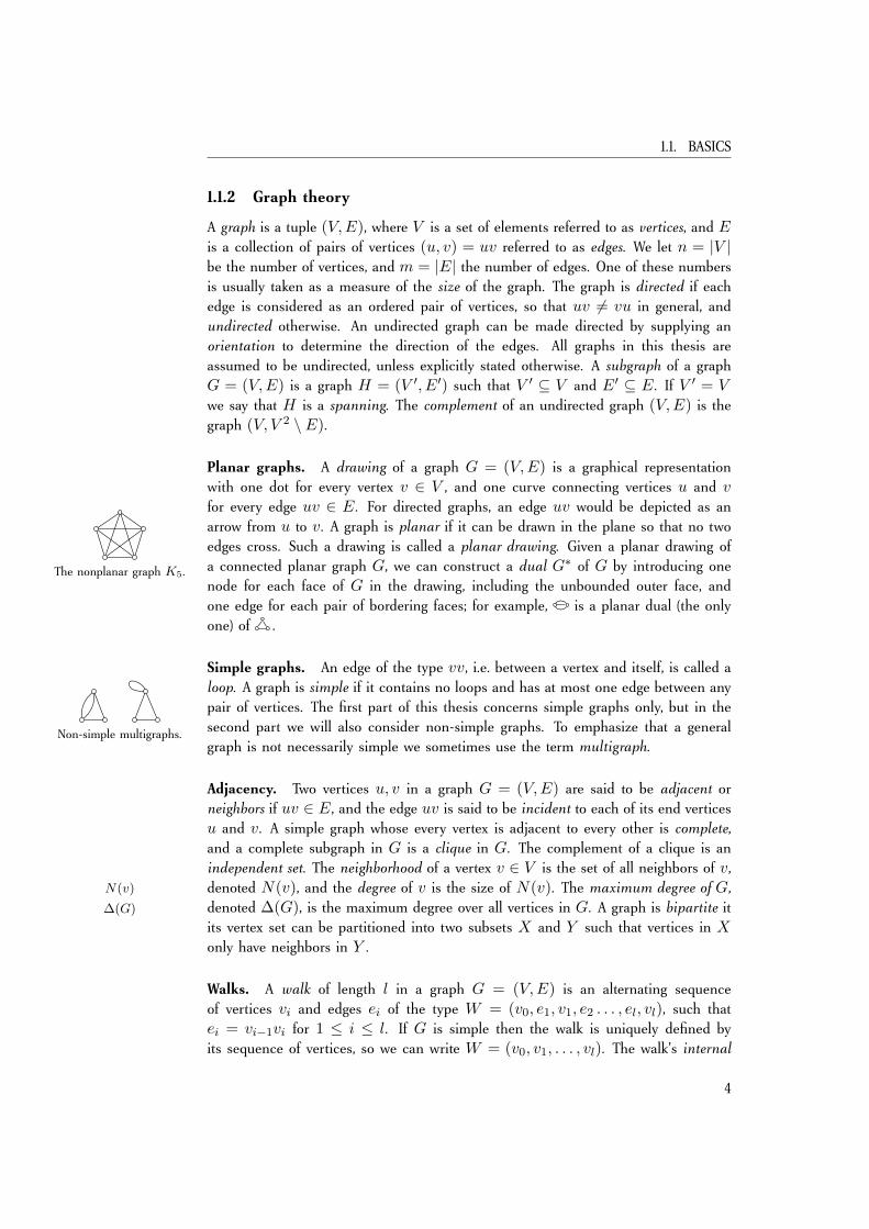
Planar graphs. A drawing of a graph G = (V,E) is a graphical representationwith one dot for every vertex v ∈ V , and one curve connecting vertices u and vfor every edge uv ∈ E. For directed graphs, an edge uv would be depicted as anarrow from u to v. A graph is planar if it can be drawn in the plane so that no twoedges cross. Such a drawing is called a planar drawing. Given a planar drawing of
The nonplanar graph K5. a connected planar graph G, we can construct a dual G∗ of G by introducing onenode for each face of G in the drawing, including the unbounded outer face, andone edge for each pair of bordering faces; for example, is a planar dual (the onlyone) of .
Simple graphs. An edge of the type vv, i.e. between a vertex and itself, is called aloop. A graph is simple if it contains no loops and has at most one edge between anypair of vertices. The first part of this thesis concerns simple graphs only, but in thesecond part we will also consider non-simple graphs. To emphasize that a generalgraph is not necessarily simple we sometimes use the term multigraph.
Non-simple multigraphs.
Adjacency. Two vertices u, v in a graph G = (V,E) are said to be adjacent orneighbors if uv ∈ E , and the edge uv is said to be incident to each of its end verticesu and v. A simple graph whose every vertex is adjacent to every other is complete,and a complete subgraph in G is a clique in G. The complement of a clique is anindependent set. The neighborhood of a vertex v ∈ V is the set of all neighbors of v,denoted N(v), and the degree of v is the size of N(v). The maximum degree of G,N(v)
denoted ∆(G), is the maximum degree over all vertices in G. A graph is bipartite it∆(G)
its vertex set can be partitioned into two subsets X and Y such that vertices in Xonly have neighbors in Y .
Walks. A walk of length l in a graph G = (V,E) is an alternating sequenceof vertices vi and edges ei of the type W = (v0, e1, v1, e2 . . . , el, vl), such thatei = vi−1vi for 1 ≤ i ≤ l. If G is simple then the walk is uniquely defined byits sequence of vertices, so we can write W = (v0, v1, . . . , vl). The walk’s internal
4

CHAPTER 1. INTRODUCTION
vertices are v1, . . . , vl−1. The walk is closed if v0 = vl, and simple if it has norepeated internal vertex.
Paths and cycles. The vertices and edges of a given walk in a graph form asubgraph that is called a cycle if the walk is closed, and a path otherwise. Notethat two simple, closed walks form the same cycle if one is a reversal, or a cyclicpermutation, of the other. An undirected graph containing no cycle is a forest. Adirected graph containing no cycle is said to be acyclic.
Connectedness. A graph is connected if any two vertices are connected by a path.A tree is a connected forest. A maximal, connected subgraph of a graph is called acomponent. The number of components of a graph (V,E) is denoted by κ(E); thus κ(E)
the graph is connected if, and only if, κ(E) = 1. A cut is a subset C ⊆ E whoseremoval increases the number of components of the graph. A singleton cut is calleda cut-edge.
Other graph structures. A k-coloring of a graph G = (V,E) is a partitioningof V into k classes (colors). A given k-coloring is said to be proper if no twoadjacent vertices are in the same color class. The chromatic number of a graph G isthe smallest number k such that G has a proper k-coloring. Proper 3-coloring.
A vertex cover of a graph G is a vertex subset such that every edge of G isincident to at least one vertex in it. A matching of G is a subset of mutuallynonadjacent edges, and a matching is perfect if it covers every vertex of G.
A k-flow in a directed graph (V,E) is an assignment φ : E 7→ ±1, . . . , k− 1to the edges, such that for any vertex v ∈ V the sum of the assigned values foroutgoing edges from v equals the sum over incoming edges to v. The number ofk-flows is independent of the edge orientation, and for an undirected graph k-flowsare considered with respect to an arbitrary fixed orientation.
1
1
2
2
−3
4-flow.
1.2 Exponential-Time Complexity
With successful advances in exponential-time algorithms, an interest in the notion ofexponential-time complexity followed naturally. For example, it would be interestingto know whether a given NP-complete problem is likely to require time exponentialin the input size n, or whether there is hope for some algorithm with subexponentialrunning time such as 2O(
√n). For such questions, the notion of NP-hardness is not
helpful, as it cannot distinguish between different superpolynomial time complexities.Instead, Impagliazzo, Paturi and Zane [57] introduced the Exponential Time Hypothesis,claiming a certain exponential-time lower bound for the problem 3-Sat,
3-Sat
Input: A 3-CNF formula ϕ with n variables and m clauses.Task: Decide whether ϕ is satisfiable.
The complexity claim is as follows.
5

1.2. EXPONENTIAL-TIME COMPLEXITY
Exponential Time Hypothesis (ETH):
There is a real number c > 0 such that no deterministic algorithmcan decide 3-Sat in time 2cn.
Later, as a consequence of the so called Sparsification lemma, the same authorsshowed that ETH would also rule out the existence of subexponential-time algorithmsfor 3-Sat in terms of the number of clauses.
Theorem 1.1 (Impagliazzo et al. [57]). Assuming ETH, there is a real number c > 0such that no deterministic algorithm can decide 3-Sat in time 2cm.
Under ETH we can get a more detailed picture of the complexity landscape withinthe class of NP-hard problems. Compared to classical complexity theory, we musthere pay more attention to any blow-up of instance sizes in a reduction, so as topreserve information about an exponential-time lower bound.
1.2.1 Parameterized complexity
Assuming ETH to be true, many NP-complete graph problems can be shown to requiretime exponential in the size of the input graph, usually measured in the number ofvertices n or edges m. However, for some problems there are other aspects, exceptthe size of the graph, that affect the complexity. For example, finding a minimumvertex cover in a general graph requires time exponential in n under ETH [57], butif we fix a number k then deciding whether the graph has a vertex cover of size atmost k is polynomial-time solvable: for every subset of k vertices—and there are(nk
)nO(1) ⊂ nO(k) such subsets—check if it forms a vertex cover.Detecting a vertex cover of given size is an example of a parameterized problem,
where part of the input is a natural number k measuring some parameter of theinput whose effect on the complexity we wish to highlight. Downey and Fellows givea systematic introduction to the theory of parameterized complexity in [32].
Fixed-parameter tractability. We can do better than the above suggested nO(k)-solution to the parameterized vertex cover problem, by first performing a certainpolynomial-time preprocessing step (see e.g. [37]) which either decides directly whetherthe input graph G has a vertex cover of size k, or returns a graph G′ of size at most2k such that G has a vertex cover of size k if, and only if, G′ has one. Then theabove brute-force approach can be applied to G′. In total, this gives a running timeof(2kk
)nO(1) ⊂ 2O(k)nO(1). This is an example of fixed-parameter tractability.
Definition 1.1. A computational problem is fixed-parameter tractable (FPT) with respectto parameter k if there is an algorithm for the problem with running time f(k)nO(1),where f is a function depending only on k, and n is the input size.
This type of complexity may be acceptable for instances where k is small comparedto n, provided the function f(k) does not grow too rapidly.
6
CHAPTER 1. INTRODUCTION
There is an analogue concept of NP-hardness for parameterized problems calledW[1]-hardness. We will not need the formal definition of the class W[1], but we notethe following result.
Theorem 1.2 (Downey and Fellows [32]). Assuming ETH, a problem that is W[1]-hardwith respect to a parameter k cannot be fixed-parameter tractable with respect to k.
Kernels. The preprocessing step mentioned above for the vertex cover problem isan example of a kernel: a mapping reduction from a parameterized problem to itself,that transforms any given instance into an equivalent instance of size f(k), for somefunction f depending only on the parameter k and referred to as the size of thekernel. For example the above vertex cover problem, parameterized by solution sizek, admits a kernel of size 2k. Such polynomial kernels are especially sought after,as they usually translate into FPT-algorithms with a decent dependency on k, suchas the 2O(k)nO(1)-time algorithm mentioned above. It can be shown (see e.g [11,Theorem 1]) that a problem admits a kernel for a parameter k if, and only if, it is alsofixed-parameter tractable with respect to k.
1.3 Overview of this thesis
Chapter 2 contains a brief review of algorithmic techniques of relevance for detectinglong cycles in graphs: dynamic programming, inclusion-exclusion, color coding, andin particular a monomial sieving technique due to Koutis and Williams [69]. Asa warm-up to Chapter 3, this monomial sieving technique is demonstrated on theproblem of detecting induced cycles in degree-bounded graphs, such that the solutionconnects a small number of terminal vertices.
Chapter 3 concerns the problem of finding a cycle through a given set of specifiedvertices and/or edges. A Monte Carlo algorithm is presented with a running time thatis exponential only in the number of specified elements. With high probability thealgorithm finds a shortest solution. It uses several techniques discussed in Chapter 2,and the correctness follows from a subtle pairing argument. This is joint workwith Andreas Björklund and Thore Husfeldt, and was published in [9]. Due to anobservation by Magnus Wahlström, this algorithm could be adjusted to also givecontrol of the parity of the length of a solution cycle. A problem concerning theparameterized complexity is discussed; this problem has now been solved by MagnusWahlström.
Chapter 4 gives an introduction to the Tutte polynomial, and to the #P-hardproblem of evaluating the Tutte polynomial of multigraphs at a given point in the(x, y)-plane. A brief survey of previous complexity results is given, especially thework by Dell et al. [30] on exponential-time complexity under #ETH, a countinganalogue of ETH.
Chapter 5 concerns the exponential-time complexity of evaluating the Tutte poly-nomial of simple graphs, in particular for points on the line x = 1 corresponding tothe reliability polynomial. In the framework proposed by Dell et al. [30] it is shown
7

1.3. OVERVIEW OF THIS THESIS
that, assuming #ETH, evaluation of the Tutte polynomial at a point with x = 1requires time exponential in Ω(m/log2m) for simple graphs of m edges, exceptfor the point (1, 1) which was already known to be polynomial-time solvable. Asthe problem is known to be solvable in vertex-exponential time for any point, thislower bound shows that the hardest instances are sparse graphs of roughly lineardensity. For y > 1 this is joint work with Thore Husfeldt, and was published in [56].Joining efforts with Holger Dell, the result was finally extended to the full line, andincorporated into the journal paper [29] which now gives asymptotically tight (up toa polylogarithmic factor in the exponent) lower bounds under #ETH for the wholeplane, except the line y = 1.
Chapter 6 concerns the exponential-time complexity of evaluating the Tutte poly-nomial of planar graphs. As an algorithm is known for this problem with a runningtime exponential only in O(
√n), the question is whether this is asymptotically op-
timal under #ETH. By analysis of existing polynomial-time reductions, this is shownto indeed be the case for general points, as a matching lower bound is found forany point on the hyperbola (x − 1)(y − 1) = 3. For remaining nontrivial pointsin the plane, lower bounds exponential in Ω(n1/k) are found for various k > 2. Inparticular, a lower bound exponential in Ω(n1/8) is given for the line y = 1. To thebest of the knowledge of the author, this is the first concrete superpolynomial lowerbound on this line also for multigraphs in general.
8

Part I
Algebraic Algorithms for CycleDetection
9

Chapter 2
Finding Cycles in Graphs
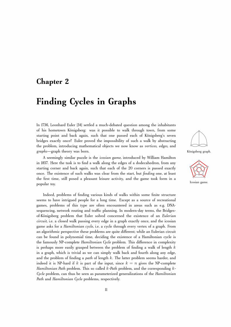
In 1736, Leonhard Euler [34] settled a much-debated question among the inhabitantsof his hometown Königsberg: was it possible to walk through town, from somestarting point and back again, such that one passed each of Königsberg’s sevenbridges exactly once? Euler proved the impossibility of such a walk by abstractingthe problem, introducing mathematical objects we now know as vertices, edges, and
Königsberg graph.graphs—graph theory was born.
A seemingly similar puzzle is the icosian game, introduced by William Hamiltonin 1857. Here the task is to find a walk along the edges of a dodecahedron, from anystarting corner and back again, such that each of the 20 corners is passed exactlyonce. The existence of such walks was clear from the start, but finding one, at leastthe first time, still posed a pleasant leisure activity, and the game took form in apopular toy. Icosian game.
Indeed, problems of finding various kinds of walks within some finite structureseems to have intrigued people for a long time. Except as a source of recreationalgames, problems of this type are often encountered in areas such as e.g. DNA-sequencing, network routing and traffic planning. In modern-day terms, the Bridges-of-Königsberg problem that Euler solved concerned the existence of an Euleriancircuit, i.e. a closed walk passing every edge in a graph exactly once, and the icosiangame asks for a Hamiltonian cycle, i.e. a cycle through every vertex of a graph. Froman algorithmic perspective these problems are quite different; while an Eulerian circuitcan be found in polynomial time, deciding the existence of a Hamiltonian cycle isthe famously NP-complete Hamiltonian Cycle problem. This difference in complexityis perhaps more easily grasped between the problem of finding a walk of length kin a graph, which is trivial as we can simply walk back and fourth along any edge,and the problem of finding a path of length k. The latter problem seems harder, andindeed it is NP-hard if k is part of the input, since k = n gives the NP-completeHamiltonian Path problem. This so called k-Path problem, and the corresponding k-Cycle problem, can thus be seen as parameterized generalizations of the HamiltonianPath and Hamiltonian Cycle problems, respectively.
11
2.1. ALGORITHMIC TECHNIQUES FOR CYCLE FINDING
2.1 Algorithmic techniques for cycle finding
Over the years, a number of interesting algorithmic techniques have evolved from, orfound nice application to, work on exact algorithms for the Hamiltonian Cycle/Pathproblem, or the k-Path/Cycle problem. This section describes four of the most influ-ential such techniques. Three of these techniques will be useful in Chapter 3, wherewe study another generalization of the Hamiltonian Cycle problem.
We will only consider the cycle-version of these problems, but the same tech-niques apply to the path-versions. Indeed, given an input graph G to the HamiltonianPath problem or the k-Path problem, we can construct a graph G′ by adding a newvertex to G and making it connected to every other vertex. Then G′ has a Hamilto-nian cycle if, and only if, G has a Hamiltonian path, and G′ has a cycle of lengthk + 1 if, and only if, G has a path of length k.
2.1.1 Dynamic programming over subsets
A brute-force solution to the Hamiltonian Cycle problem enumerates all permutationsof the vertices, and checks for each permutation whether it defines a closed walk inthe graph. The resulting running time is thus n!nO(1). This upper bound was dra-matically improved in 1962, when Bellman [5] and Held and Karp [53] independentlydiscovered the following algorithm based on dynamic programming:
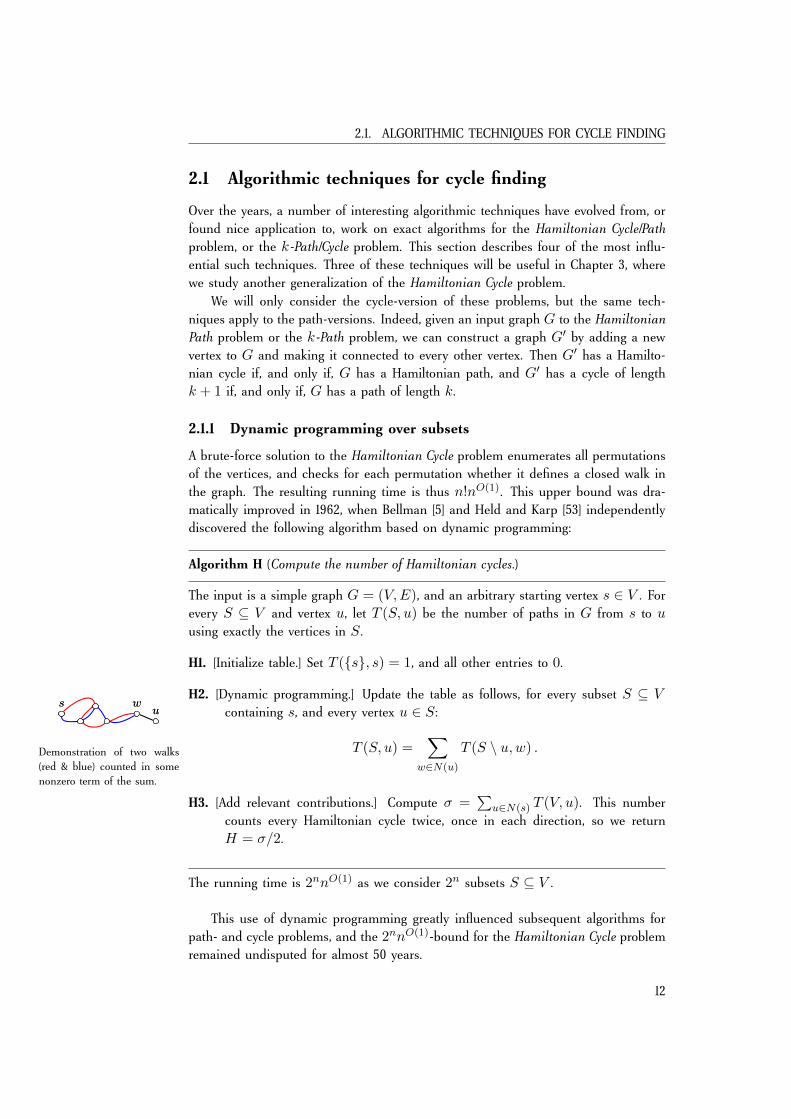
Algorithm H (Compute the number of Hamiltonian cycles.)
The input is a simple graph G = (V,E), and an arbitrary starting vertex s ∈ V . Forevery S ⊆ V and vertex u, let T (S, u) be the number of paths in G from s to uusing exactly the vertices in S.
H1. [Initialize table.] Set T (s, s) = 1, and all other entries to 0.
H2. [Dynamic programming.] Update the table as follows, for every subset S ⊆ Vcontaining s, and every vertex u ∈ S:
T (S, u) =∑
w∈N(u)
T (S \ u,w) .
s wu
s wu
Demonstration of two walks(red & blue) counted in somenonzero term of the sum.
H3. [Add relevant contributions.] Compute σ =∑
u∈N(s) T (V, u). This numbercounts every Hamiltonian cycle twice, once in each direction, so we returnH = σ/2.
The running time is 2nnO(1) as we consider 2n subsets S ⊆ V .
This use of dynamic programming greatly influenced subsequent algorithms forpath- and cycle problems, and the 2nnO(1)-bound for the Hamiltonian Cycle problemremained undisputed for almost 50 years.
12
CHAPTER 2. FINDING CYCLES IN GRAPHS
2.1.2 The principle of inclusion and exclusion
An issue with the above dynamic programming solution is that except for exponentialtime, it also requires exponential space. A way around this is the following technique,based on the principle of inclusion and exclusion.
For S ⊆ V , let AS be the set of closed walks of length n, starting and ending atsome given vertex s, that avoid all vertices in S. Then the number H of Hamiltoniancycles satisfies
2H = |A∅| = |⋃u∈V
Au|
=∑S⊆V
(−1)|S||⋂u∈S
Au|
=∑S⊆V
(−1)|S||AS | , (2.1)
where the second equality follows from the principle of inclusion and exclusion; seee.g. (9) in [55]. Again, every Hamiltonian cycle is counted twice in |A∅| (once ineach direction). We compute each value |AS | by dynamic programming similar toAlgorithm H: for every u ∈ V and k ≤ n − 1, compute the number TS(k, u) ofwalks of length k from some starting vertex s to u that avoid the vertices in S , untilwe can return |AS | =
∑u∈N(s) TS(n − 1, u). Note that for each subset S ⊆ V ,
the table TS only requires quadratic space, and we only need to keep one such tableat a time in memory, while still obtaining the time bound 2nnO(1).
This idea has been reinvented many times (see e.g. [67, 61, 4]) until the generaltechnique gained popular attention in recent years; see [55] for an overview of appli-cations. A variant of this technique is used in Björklund’s 1.657nnO(1)-time MonteCarlo algorithm [6] for the Hamiltonian Cycle problem—the first algorithm to beatthe longstanding bound of 2nnO(1).
2.1.3 Color coding
For the k-Cycle problem, the brute-force solution has an upper bound of O(nk): foreach choice of k vertices, check whether they constitute a simple cycle in the graph.Monien [80] gave an algorithm with running time k!nO(1), showing the problem tobe fixed-parameter tractable with respect to the parameter k. Considering the known2nnO(1)-time algorithm for the Hamiltonian Cycle problem, a natural question waswhether the factorial dependency on k of Monien’s algorithm could be improved toexponential. Alon, Yuster and Zwick [1] provided a positive answer to this question,giving a 5.44knO(1)-time randomized algorithm for the problem, and a deterministicversion in time cknO(1) for some large constant c, by introducing the technique ofcolor coding.
The idea of color coding is to pick a random k-coloring of the vertices, c : V →[k], and then to look for a colorful k-cycle, i.e. a cycle containing exactly one vertexof each color. For any given such coloring c we can again use dynamic programming
13
2.1. ALGORITHMIC TECHNIQUES FOR CYCLE FINDING
similar to Algorithm H to count the number of colorful k-cycles: for every subsetS ⊆ [k] and vertex pair u, v ∈ V , compute the number T (S, u, v) of colorful pathsfrom u to v that uses exactly the colors from S , each color exactly once. If the graphcontains a k-cycle, then it has probability k!/kk > 1/ek of becoming colorful by arandom k-coloring, so an expected number of O(ek) colorings are needed to detectit. Hence the expected time to find an existing k-cycle is ek2knO(1) ∈ 5.44knO(1).
This technique proved successful for finding other types of subgraphs as well, andmoreover had the benefit of easily extending to weighted graphs. It was successfullyapplied for identifying certain interaction chains in protein interaction networks [86,88], which renewed the interest in efficient algorithms for the k-Cycle problem.
2.1.4 Monomial sieving
The next question was whether the base of the exponential term in the new upperbound for the k-Cycle problem could be replaced by 2, as for the classical algorithmfor the Hamiltonian Cycle problem. A Monte Carlo algorithm satisfying this was even-tually found by Williams [97], by refining an algebraic ‘sieving’ technique introducedby Koutis [68]. The idea is to associate a certain polynomial with the graph, such thatevery term corresponds to a walk of length k, and such that a term is multilinear, i.e.contains no squared variable, if, and only if, the corresponding walk is simple.1 Whilethis polynomial is easily defined implicitly, for example as a recursion, it would notbe practical to compute the expanded form; indeed, there mere number of terms tocheck would exceed the wanted time bound. Instead the following theorem is used toprobabilistically sieve the given polynomial for monomials corresponding to k-cycles.
Theorem 2.1 (Koutis, Williams [69]). Let p(x1, . . . , xt) be a polynomial of degree atmost k, and suppose p can be represented by an arithmetic circuit of size polynomialin t, with no scalar multiplications. Then the existence of a multilinear term in p canbe decided by a Monte Carlo algorithm in time 2ktO(1), with small probability of afalse negative.
In short, the algorithm uses the arithmetic circuit, typically a dynamic program-ming formulation, to evaluate the polynomial at a random point of coordinates froma certain group algebra over a finite field Fq , such that any square evaluates to zeroin this algebra. The remaining sum, corresponding to multilinear terms, will thenevaluate to something nonzero with a probability given by the following lemma:
Lemma 2.1 (DeMillo-Lipton-Schwartz-Zippel). Let p ∈ Fq[x1, . . . , xt] be a nonzeropolynomial of total degree at most d. Then, for r1, r2, . . . , rt ∈ Fq selected indepen-dently and uniformly at random,
Pr[ p(r1, r2, . . . , rt) 6= 0 ] ≥ 1− d
q.
1The idea of associating a polynomial with a certain structure we want to find goes back to Tutte [91],who noted that a graph has a perfect matching if, and only if, the determinant of a certain matrix withvariable entries is a nonzero polynomial. Lovász [79] was the first to realize the algorithmic potential ofthis result, when coupled with the DeMillo-Lipton-Schwartz-Zippel lemma.
14
CHAPTER 2. FINDING CYCLES IN GRAPHS
The probability of a false negative in Theorem 2.1 decreases exponentially withthe number of such random evaluations of the given polynomial, with a rate thatdepends on the size of the chosen field Fq but not on k. The exponential term ofthe running time comes from the cost of arithmetic operations in the group algebra.
This approach to the k-Cycle problem inspired Björklund to the breakthroughalgorithm for the Hamiltonian Cycle problem [6], and by further development also ledto algorithms for a number of packing problems [8]. The result of Chapter 3 is alsoinspired by this work.
2.2 Monomial sieving in action
As a warm-up to Chapter 3, this section demonstrates a somewhat elaborate applica-tion of the above monomial sieving technique.
A subgraph of a given graph G is said to be induced if it can be obtained fromG by a sequence of vertex deletions. In particular, an induced cycle in a graph G is acycle C containing no chord in G, i.e. an edge connecting two nonadjacent verticeson C . And induced cycle of length at least four is called a hole. A hole is odd oreven according to the parity of its length.
It is a curious fact that, whereas we know how to decide in polynomial timewhether a graph contains an even hole [24, 23, 21], it is still open whether oddholes can be detected in polynomial time. This problem received much interest overthe years due to the Strong Perfect Graph Conjecture, which claimed that a graph isperfect2 if, and only if, either itself or its complement contains an odd hole. Thiswas finally proved by Chudnovsky et al. [22], yielding a complete characterization ofperfect graphs, and also a polynomial-time algorithm for the problem, as it turnedout that the problem of detecting either an odd hole or the complement of an oddhole is polynomial-time solvable [20]. This makes the unclear complexity of detectingodd holes quite intriguing.
Now suppose we want to check for odd holes in a graph of bounded degree. Wewill demonstrate how Theorem 2.1 can be used to do this, while also requiring thehole to pass through a small set of specified vertices. Thus we define the followingproblem.
∆d-l-K-Hole
Input: A simple graph G = (V,E) with n vertices, maximum degree d,a specified subset K ⊂ V of size k = (log n)O(1),and a number l ≥ 3.
Task: Decide whether G contains an induced cycle of length l,containing all vertices in K .
2A graph G is said to be perfect if the chromatic number of each induced subgraph H in G is thesize of the biggest clique in H .
15
2.2. MONOMIAL SIEVING IN ACTION
The Monte Carlo algorithm resulting from Theorem 2.1 will have a running time of2dlnO(1). This is not very interesting in itself, as the problem can be solved intime 2l log dnO(1) by simple branching, but the construction here serves to introduceseveral technical aspects we will encounter in Chapter 3.
2.2.1 Monomial sieving for induced cycle detection
To apply Theorem 2.1, we seek a polynomial p associated with any input graphG, such that p has a multilinear term if, and only if, the graph G contains aninduced cycle of length l through the specified vertices in K , and such that p canbe represented by a commutative arithmetic circuit of size polynomial in the numberof variables. The running time of the algorithm will be exponential in the degree ofthe polynomial p.
Defining the polynomial. For a given graph G = (V,E) of n vertices and medges, and a specified subset K ⊂ V of size at most (log n)O(1), we construct apolynomial p as follows:
Introduce a variable xv for every vertex v ∈ V , and a variable ye for everyedge e ∈ E. For any v ∈ V , let I(v) denote the set of incident edges to v. To eachclosed walk W = (v0, v1, . . . , vl−1, v0) in G, we associate the monomial m(W ) ofdegree at most dl given by
m(W ) =
xv0 ∏e∈I(v0)e6=vl−1v0
ye
·xv1 ∏
e∈I(v1)e6=v0v1
ye
. . .
xvl−1
∏e∈I(vl−1)e6=vl−2vl−1
ye
. (2.2)
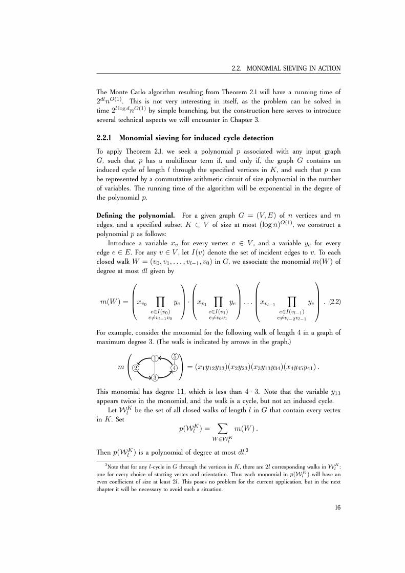
For example, consider the monomial for the following walk of length 4 in a graph ofmaximum degree 3. (The walk is indicated by arrows in the graph.)
m
1
2
3
4
5 = (x1y12y13)(x2y23)(x3y13y34)(x4y45y41) .
This monomial has degree 11, which is less than 4 · 3. Note that the variable y13appears twice in the monomial, and the walk is a cycle, but not an induced cycle.
Let WKl be the set of all closed walks of length l in G that contain every vertex
in K . Setp(WK
l ) =∑
W∈WKl
m(W ) .
Then p(WKl ) is a polynomial of degree at most dl.3
3Note that for any l-cycle in G through the vertices in K , there are 2l corresponding walks inWKl :
one for every choice of starting vertex and orientation. Thus each monomial in p(WKl ) will have an
even coefficient of size at least 2l. This poses no problem for the current application, but in the nextchapter it will be necessary to avoid such a situation.
16
CHAPTER 2. FINDING CYCLES IN GRAPHS
Correctness. We now argue that it is sufficient to look for multilinear terms in thepolynomial p(WK
l ).
Lemma 2.2. The polynomial p(WKl ) contains a multilinear term if, and only if, G
contains an l-hole containing every vertex in K .
Proof. Let W ∈ WKl . If W is not a cycle, then it contains some repeated internal
vertex v, yielding a square variable x2v in m(W ). If W is a cycle, but not induced(as in the above example), then there will be some chord of W , i.e. an edge e ∈ Eincident to two vertices vi and vj on W with |i−j| > 1 (indices considered modulol). The corresponding edge variable ye will be counted twice, in the ith and jthfactor of m(W ), yielding a square factor y2e . Thus, if W is not an induced cycle,then m(W ) is not multilinear.
Now suppose W is an induced cycle in G. Being a cycle, W will pass novertex more than once, so m(W ) is linear in every node variable xv . Being induced,there are only two ways in which an edge e ∈ E can have an endpoint on W :either e is incident to only one vertex vi of W , or e = vivi+1 for two consecutivevertices vi, vi+1 of W (indices considered modulo l). In either case the variable yeappears only once in m(w), in the ith factor. Thus m(W ) is linear also in everyedge variable ye—it is a multilinear term in p(WK
l ).
Arithmetic circuit. Then we show how to evaluate the polynomial efficiently.
Lemma 2.3. The polynomial p(WKl ) can be represented by an arithmetic circuit of
size polynomial in the number of variables.
Proof. We give a dynamic programming formulation of the polynomial p(WKl ).
For every closed walk W ∈ WKl , we would like to build the monomial m(W )
from smaller monomials corresponding to subwalks of W . To this end we define, forany walk W = (v0, v1, . . . , vr−1, vr), the monomial
m(W ) =
xv0 ∏e∈I(v0)
ye
·xv1 ∏
e∈I(v1)e6=v0v1
ye
. . .
xvr ∏e∈I(vr)e6=vr−1vr
ye
. (2.3)
Note that if vr ∈ N(v0), so that we can append the edge e = vrv0 to the end of Wto form a closed walk W ′, then m(W ) = yvr−1v0 ·m(W ′).
For all lengths r ≤ l, vertices u, v ∈ V , and subsets S ⊆ K , let WSr [u, v] be
the set of walks of length r from u to v passing every vertex of S , and set
T (r, u, v, S) =∑
W∈WSr [u,v]
m(W ) .
17
2.2. MONOMIAL SIEVING IN ACTION
We have
p(WKl ) =
∑W∈WK
l
m(W )
=∑v∈V
∑u∈N(v)
∑W∈WK
l−1[u,v]
m(W )
yuv
=∑v∈V
∑u∈N(v)
T (l − 1, v, u,K)/yuv . (2.4)
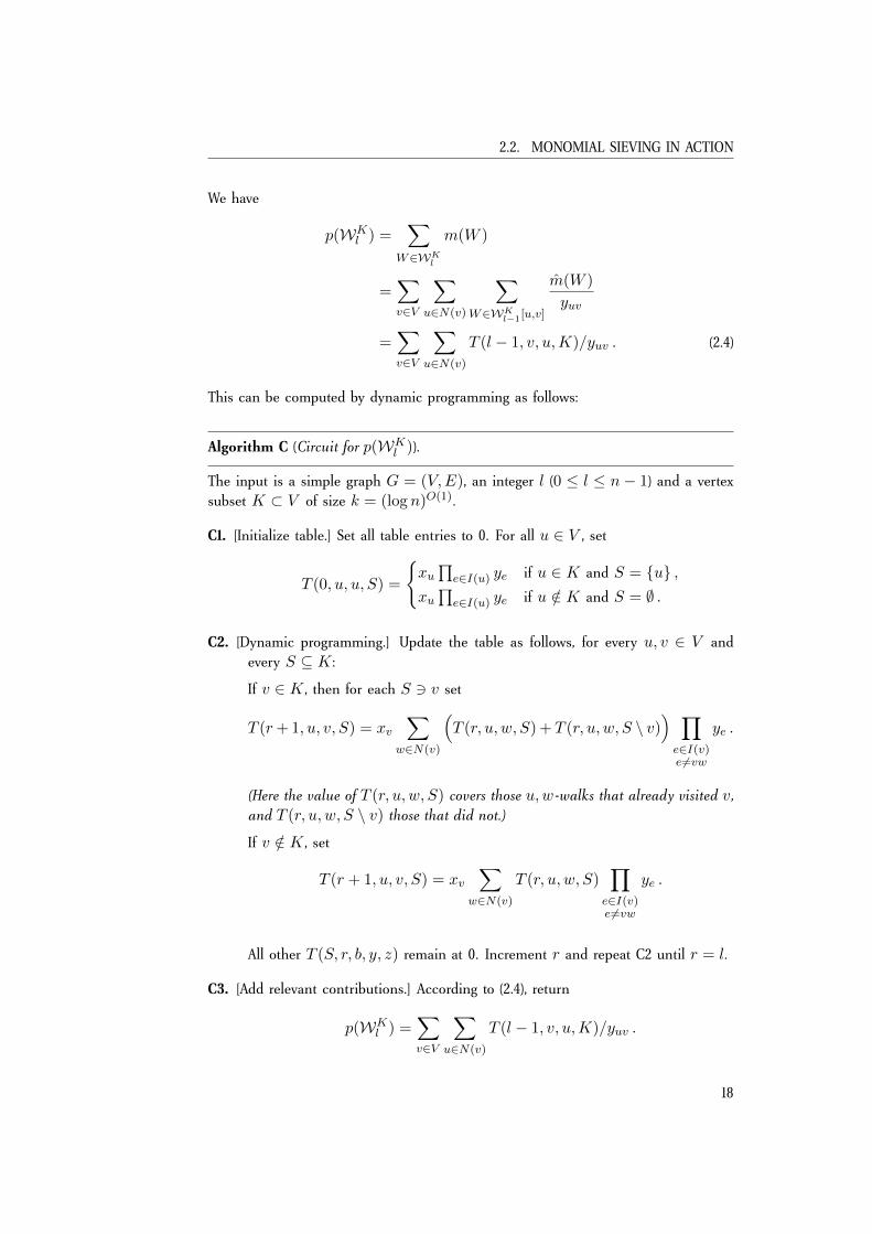
This can be computed by dynamic programming as follows:
Algorithm C (Circuit for p(WKl )).
The input is a simple graph G = (V,E), an integer l (0 ≤ l ≤ n− 1) and a vertexsubset K ⊂ V of size k = (log n)O(1).
C1. [Initialize table.] Set all table entries to 0. For all u ∈ V , set
T (0, u, u, S) =
xu∏e∈I(u) ye if u ∈ K and S = u ,
xu∏e∈I(u) ye if u /∈ K and S = ∅ .
C2. [Dynamic programming.] Update the table as follows, for every u, v ∈ V andevery S ⊆ K :
If v ∈ K , then for each S 3 v set
T (r+ 1, u, v, S) = xv∑
w∈N(v)
(T (r, u, w, S) + T (r, u, w, S \ v)
) ∏e∈I(v)e6=vw
ye .
(Here the value of T (r, u, w, S) covers those u,w-walks that already visited v,and T (r, u, w, S \ v) those that did not.)
If v /∈ K , set
T (r + 1, u, v, S) = xv∑
w∈N(v)
T (r, u, w, S)∏e∈I(v)e6=vw
ye .
All other T (S, r, b, y, z) remain at 0. Increment r and repeat C2 until r = l.
C3. [Add relevant contributions.] According to (2.4), return
p(WKl ) =
∑v∈V
∑u∈N(v)
T (l − 1, v, u,K)/yuv .
18
CHAPTER 2. FINDING CYCLES IN GRAPHS
This gives an arithmetic circuit for p(WKl ) of size O(2kn2d2), which is polyno-
mial in n + m since k = (log n)O(1) by assumption. The number of variables ofp(WK
l ) is n+m.
Thus Lemma 2.2 and Lemma 2.3 shows that the polynomial p(WKl ) satisfies the
assumptions in Theorem 2.1. As the degree of the polynomial is dl, this yields a2dlnO(1)-time Monte Carlo algorithm for the problem ∆d-l-K-Hole.
19
2.2. MONOMIAL SIEVING IN ACTION
20
Chapter 3
Finding Cycles Through SpecifiedElements
smile smite spite suite quite quire
shamesharescarescarssearstears
quirt
quilt
guilt
guile
guide
glide
slide
slime
clime
crime
prime
pride
price
prick
crick
crock
crookgrookgroomgloombloombloodbrood
broad bread dread tread treed trees
trews
trows
trots
toots
torts
worts
words
wordy
worry
wormy
worms
forms
foams
flams
slams
shamsshame
spite
guilt
pride
gloom
dread
worry
tears
smile
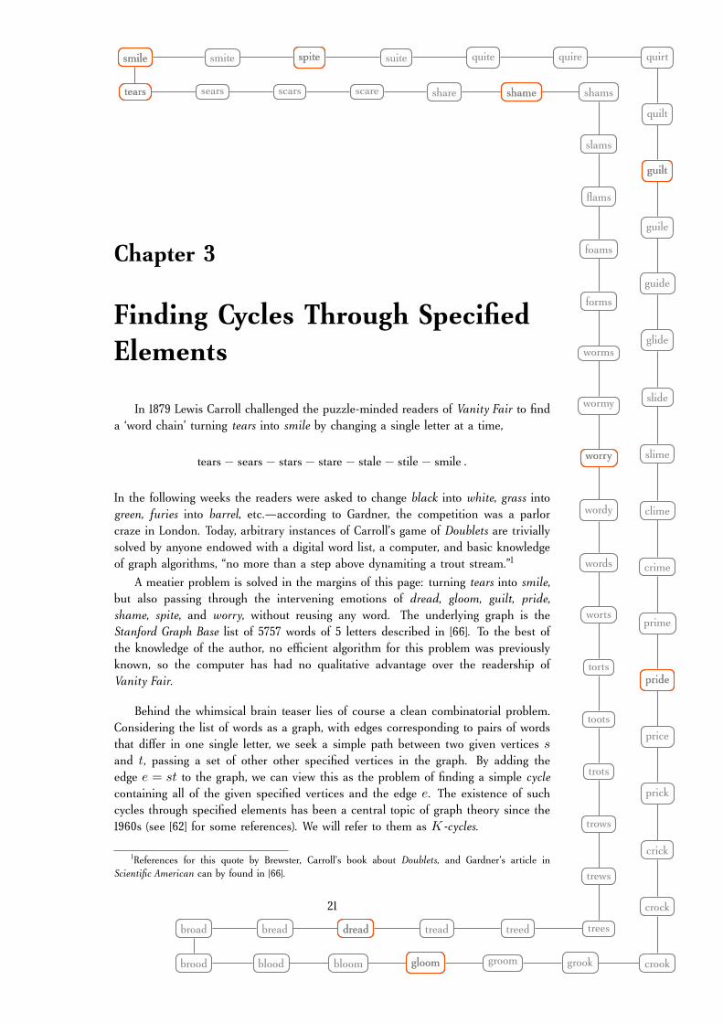
In 1879 Lewis Carroll challenged the puzzle-minded readers of Vanity Fair to finda ‘word chain’ turning tears into smile by changing a single letter at a time,
tears− sears− stars− stare− stale− stile− smile .
In the following weeks the readers were asked to change black into white, grass intogreen, furies into barrel, etc.—according to Gardner, the competition was a parlorcraze in London. Today, arbitrary instances of Carroll’s game of Doublets are triviallysolved by anyone endowed with a digital word list, a computer, and basic knowledgeof graph algorithms, “no more than a step above dynamiting a trout stream.”1
A meatier problem is solved in the margins of this page: turning tears into smile,but also passing through the intervening emotions of dread, gloom, guilt, pride,shame, spite, and worry, without reusing any word. The underlying graph is theStanford Graph Base list of 5757 words of 5 letters described in [66]. To the best ofthe knowledge of the author, no efficient algorithm for this problem was previouslyknown, so the computer has had no qualitative advantage over the readership ofVanity Fair.
Behind the whimsical brain teaser lies of course a clean combinatorial problem.Considering the list of words as a graph, with edges corresponding to pairs of wordsthat differ in one single letter, we seek a simple path between two given vertices sand t, passing a set of other other specified vertices in the graph. By adding theedge e = st to the graph, we can view this as the problem of finding a simple cyclecontaining all of the given specified vertices and the edge e. The existence of suchcycles through specified elements has been a central topic of graph theory since the1960s (see [62] for some references). We will refer to them as K-cycles.
1References for this quote by Brewster, Carroll’s book about Doublets, and Gardner’s article inScientific American can by found in [66].
21
3.1. THE K-CYCLE PROBLEM
3.1 The K-Cycle problem
For a graph G = (V,E) and a set K ⊆ V ∪ E of specified vertices or edges, aK-cycle in G is a simple cycle that includes all elements of K . By the parity of aK-cycle we refer to the parity of its length. We define the K-Cycle problem as follows,
K-Cycle
Input: A simple graph G = (V,E) with n vertices,and a subset K ⊆ V ∪ E of size k.
Task: Decide whether G contains a K-cycle.
We can restrict our attention to the case where K contains only vertices; indeed,any specified edge uv can be replaced by adding a fresh vertex w to K and V andadding the edges uw and wv to E. This increases n by at most k.
The K-Cycle problem can be seen as a generalization of the Hamiltonian Cycleproblem, corresponding to the case K = V . Consequently, the problem is NP-hardin general, and assuming ETH it cannot be solved in time 2o(k)nO(1) [57].
3.1.1 Relation to the Disjoint Paths problem
The K-Cycle problem has an interesting relation to the following well-known problem.
Disjoint Paths
Input: A simple graph G = (V,E) with n vertices,and a set of k vertex pairs (s1, t1), . . . , (sk, tk).
Task: Decide whether G contains k paths P1, . . . , Pk , pairwise disjointexcept possible overlapping endpoints, such that Pi connects si to ti.
This problem is central in areas such as high-speed network routing and trans-portation networks; see [42] for a survey of applications. It was a seminal resultof Robertson and Seymour’s Graph Minors Project that the Disjoint Paths problem isfixed-parameter tractable with respect to the number k of terminal pairs [85]. Wehave the following connection to the K-Cycle problem:
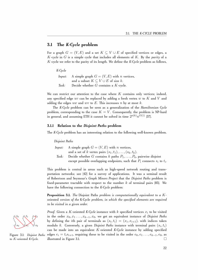
Proposition 3.1. The Disjoint Paths problem is computationally equivalent to a K-oriented version of the K-Cycle problem, in which the specified elements are requiredto be visited in a given order.
Proof. Given a K-oriented K-Cycle instance with k specified vertices xi to be visitedin the order x0, x1 . . . , xk−1, x0, we get an equivalent instance of Disjoint Pathsby defining the ith pair of terminals as (si, ti) = (xi, xi+1), with indices takenmodulo k. Conversely, a given Disjoint Paths instance with terminal pairs (si, ti)
t0 t1 t2
s0 s1 s2
Figure 3.1: Disjoint Pathsto K-oriented K-Cycle.
can be made into an equivalent K-oriented K-Cycle instance by adding specifiededges ei = tisi+1, requiring these to be visited in the order e0, e1 . . . , ek−1, e0, asillustrated in Figure 3.1.
22
CHAPTER 3. FINDING CYCLES THROUGH SPECIFIED ELEMENTS
From this connection it is immediate from Robertson and Seymour’s result thatthe K-Cycle problem is fixed-parameter tractable with respect to the number of spec-ified elements: simply consider each possible order to visit the k specified elements.Thus we know that the problem can be solved in time f(k)nO(1) for some functionf(k). This should, however, be considered a theoretical result, as the time depen-dency on k that follows implicitly from Robertson and Seymour’s constructions isquite extreme, involving repeated exponentiation and tower functions, which makes itcompletely impractical for any value of k. The first improvement over this was givenrecently by Kawarabayashi [62], with an algorithm whose dependency on k is doublyexponential in k10.
3.1.2 Main theorem
Section 3.2 presents a Monte Carlo algorithm for an optimization version of the K-Cycle problem, with a running time that matches the exponential-time lower boundunder ETH. The author is obliged to Magnus Wahlström for observing that the algo-rithm also solves a parity version of the problem.
Theorem 3.1. Let G be an n-vertex graph, and K a set of k specified vertices of edgesin G. A K-cycle of given parity in G can be found by a Monte Carlo algorithm intime 2knO(1), with a small probability of a false negative, or of a solution that is notshortest possible.
The problem of determining the length of a shortest K-cycle was not known tobe fixed-parameter tractable, to the best of the knowledge of the author.
Note that this result is an improvement not only in the theoretical sense. Whereasprevious algorithms would outperform the brute force solution only for inputs ofgalactic size, a straightforward implementation of the algorithm in Section 3.2 isable to find cycles through several specified elements in a graph with thousands ofvertices. Also, the algorithm is short and conceptually simple, using nothing morecomplicated than dynamic programming. The correctness argument is a bit moresubtle, but except for the DeMillo-Lipton-Schwartz-Zippel lemma, the presentation isself-contained.
If the graph has no K-cycle of the given parity, the algorithm will never report afalse positive. If the graph has a K-cycle of the given parity, then such a cycle willbe found with high probability, and it will be shortest possible with high probability.
3.1.3 Related work
The K-Cycle problem. For k = 1, the problem can be solved by breadth firstsearch, and for k = 2 it corresponds to detecting two vertex-disjoint paths betweenthe specified vertices, which is solvable by an adaption of the Ford-Fulkerson method;see e.g. [16, Chapter 9.1]. For k = 3, it can be solved in linear time by a dedicatedalgorithm [36, 73]. The mentioned algorithm by Kawarabayashi [62], involving someof the ideas of Robertson and Seymour [85], finds a cycle through k specified edges
23
3.1. THE K-CYCLE PROBLEM
in polynomial time provided k ∈ O((log logn)1/10). This remains the best knowndeterministic algorithm for general k.
The arguments needed to establish the correctness of previous algorithms for k ≥3 are complicated. The k = 3 algorithm by [73] requires extensive case analysispartially omitted from the journal version and appearing only in [72]. The other algo-rithms rely on combinatorial results, in the extreme case of Robertson and Seymour’salgorithm [85] the correctness proof requires hundreds of pages.
For directed graphs, the case k = 1 is solved as for undirected graphs, but alreadythe detection problem for k = 2 is NP-hard [41].
Shortest K-cycle. For the optimization problem of finding a shortest K-cycle, littlewas known. Dean’s list of open questions from a 1991 conference on graph minors[27] asks if the problem can be solved in polynomial time for fixed k; i.e. if theproblem is fixed-parameter tractable with respect to k. For k = 2, the problem is aspecial case of minimum-cost network flow and solvable by textbook algorithms; see[90] for some early results. According to [27], the case k = 3 is solved by Fleischnerand Woeginger in [36], though this is not made explicit. An algorithm for fixed k > 3does not follow from Robertson-Seymour techniques, and the question seems to haveremained open.
K-cycle of given parity. Kawarabayashi, Li, and Reed [64] give an algorithm fordetecting a K-cycle of given parity. For fixed k the running time is polynomial in n,so the problem was known to be fixed-parameter tractable with respect to k, but thedependency on k is not given.
K-cycle of given length. The brute-force way to find a K-cycle of length l is ofcourse to consider all
(nl
)candidate vertex subsets in G and see if they describe a
K-cycle. Algorithms for long paths whose running time is exponential in the pathlength are known, and it is easy to change these algorithm to consider only suchpaths that visit K , as for the algorithm described in Section 2.2. For example, thealgorithm in [8] can be modified to detect a K-cycle of length l in time 1.66lnO(1).While this may be competitive with previous algorithms for the he K-Cycle problemfor k > 3, it would for example be time-consuming to find the solution on the titlepage, which has l = 58. Moreover, it seems difficult to modify these algorithms tobe able to detect the absence of a K-cycle in time subexponential in n.
Induced K-cycle. Kobayashi and Kawarabayashi [63] give an algorithm for detect-ing an induced K-cycle in a planar graph in time wO(w)n2, where w = k2/3. Inparticular, their algorithm runs in polynomial time for k = o((log n/ log log n)2/3).For general graphs, this problem is NP-complete even for k = 2, and the ideas of thischapter do not seem to easily lend themselves to this induced version of the problem.
24
CHAPTER 3. FINDING CYCLES THROUGH SPECIFIED ELEMENTS
3.1.4 Technique
The algorithm presented in this chapter uses the monomial sieving idea discussed inthe previous chapter. Compared to other recent papers using this technique, such as[6, 8, 69, 97], the construction here is quite simple, but the analysis is more delicate.
One could view the determinant summation technique of [6], for the HamiltonianCycle problem, as detecting a cycle of length n through n/2 specified elements. Therunning time there is exponential in the number of vertices between the specifiedones. For the algorithm below the situation is reversed: the specified vertices areexponentially expensive, and the vertices in-between are cheap.
3.2 Algorithm
We first introduce some relevant concepts.
3.2.1 Terminology and definitions
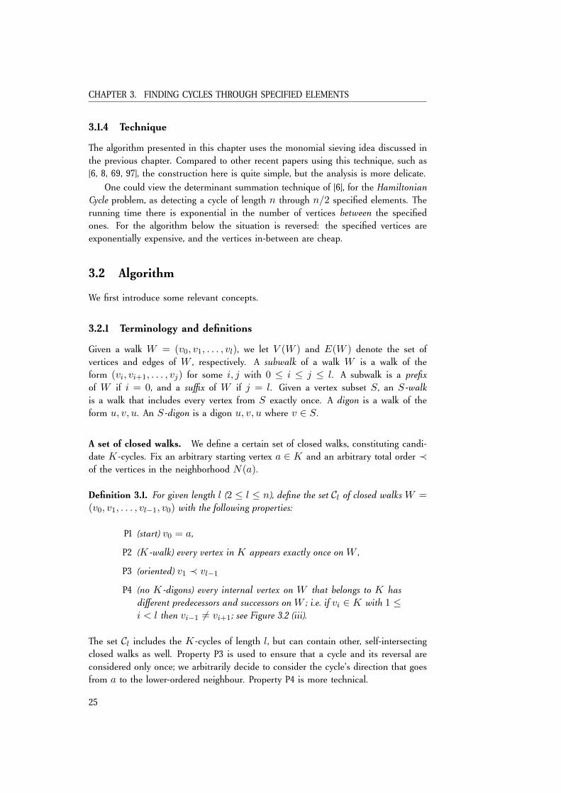
Given a walk W = (v0, v1, . . . , vl), we let V (W ) and E(W ) denote the set ofvertices and edges of W , respectively. A subwalk of a walk W is a walk of theform (vi, vi+1, . . . , vj) for some i, j with 0 ≤ i ≤ j ≤ l. A subwalk is a prefixof W if i = 0, and a suffix of W if j = l. Given a vertex subset S , an S-walkis a walk that includes every vertex from S exactly once. A digon is a walk of theform u, v, u. An S-digon is a digon u, v, u where v ∈ S.
A set of closed walks. We define a certain set of closed walks, constituting candi-date K-cycles. Fix an arbitrary starting vertex a ∈ K and an arbitrary total order ≺of the vertices in the neighborhood N(a).
Definition 3.1. For given length l (2 ≤ l ≤ n), define the set Cl of closed walks W =(v0, v1, . . . , vl−1, v0) with the following properties:
P1 (start) v0 = a,
P2 (K-walk) every vertex in K appears exactly once on W ,
P3 (oriented) v1 ≺ vl−1P4 (no K-digons) every internal vertex on W that belongs to K has
different predecessors and successors on W ; i.e. if vi ∈ K with 1 ≤i < l then vi−1 6= vi+1; see Figure 3.2 (iii).
The set Cl includes the K-cycles of length l, but can contain other, self-intersectingclosed walks as well. Property P3 is used to ensure that a cycle and its reversal areconsidered only once; we arbitrarily decide to consider the cycle’s direction that goesfrom a to the lower-ordered neighbour. Property P4 is more technical.
25
3.2. ALGORITHM
a
b y z
x
(i)
N(a)
a
v1
vl−1
(ii)
vi−1 vi+1
vi
(iii)
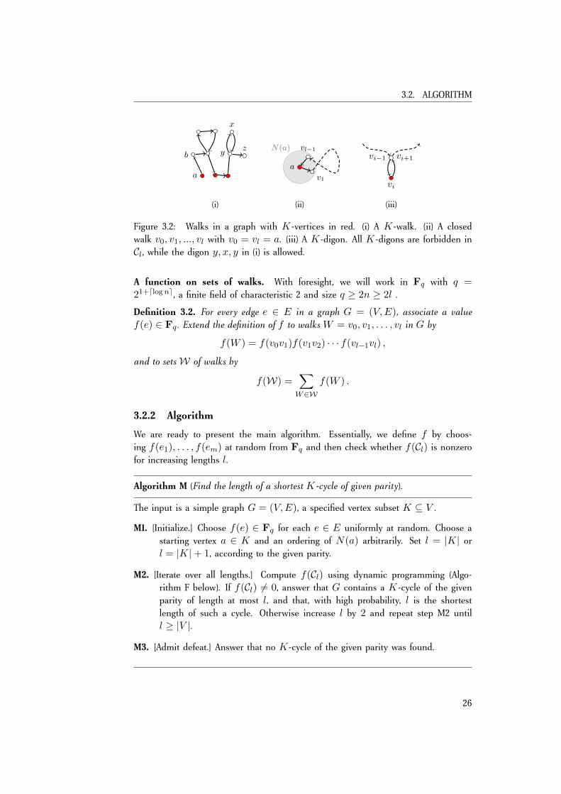
Figure 3.2: Walks in a graph with K-vertices in red. (i) A K-walk. (ii) A closedwalk v0, v1, ..., vl with v0 = vl = a. (iii) A K-digon. All K-digons are forbidden inCl, while the digon y, x, y in (i) is allowed.
A function on sets of walks. With foresight, we will work in Fq with q =21+dlogne, a finite field of characteristic 2 and size q ≥ 2n ≥ 2l .
Definition 3.2. For every edge e ∈ E in a graph G = (V,E), associate a valuef(e) ∈ Fq . Extend the definition of f to walks W = v0, v1, . . . , vl in G by
f(W ) = f(v0v1)f(v1v2) · · · f(vl−1vl) ,
and to setsW of walks by
f(W) =∑W∈W
f(W ) .
3.2.2 Algorithm
We are ready to present the main algorithm. Essentially, we define f by choos-ing f(e1), . . . , f(em) at random from Fq and then check whether f(Cl) is nonzerofor increasing lengths l.
Algorithm M (Find the length of a shortest K-cycle of given parity).
The input is a simple graph G = (V,E), a specified vertex subset K ⊆ V .
M1. [Initialize.] Choose f(e) ∈ Fq for each e ∈ E uniformly at random. Choose astarting vertex a ∈ K and an ordering of N(a) arbitrarily. Set l = |K| orl = |K|+ 1, according to the given parity.
M2. [Iterate over all lengths.] Compute f(Cl) using dynamic programming (Algo-rithm F below). If f(Cl) 6= 0, answer that G contains a K-cycle of the givenparity of length at most l, and that, with high probability, l is the shortestlength of such a cycle. Otherwise increase l by 2 and repeat step M2 untill ≥ |V |.
M3. [Admit defeat.] Answer that no K-cycle of the given parity was found.
26
CHAPTER 3. FINDING CYCLES THROUGH SPECIFIED ELEMENTS
This algorithm establishes Theorem 3.1. The proof of correctness is in Section 3.3.Note that if the algorithm reports a K-cycle at length l, then this is probably the
length of a shortest K-cycle, but as we will see there is a possibility that a shorterK-cycle was missed on a previous iteration, i.e., that we got a false negative at thatiteration. The probability of this situation is bounded by a fixed number p < 1/2,just as the probability of a false negative in general, and we can simply repeat thealgorithm until we are sufficiently confident of the answer.
Dynamic programming. The values f(Cl) in step M2 can be computed usingdynamic programming over the subsets of K and the length of the walk’s prefix, in asimilar vein as Algorithm H in the previous chapter. We only need to maintain someextra information about the last two vertices on a walk’s prefix (in order to avoidbuilding an K-digon) and the second vertex (in order to determine the orientation ofthe final closed walk), as follows.
For every vertex subset S ⊆ K , vertices b, y, z ∈ V , and length r ≤ n − 1,define the values
T (S, r, b, y, z) =∑
W∈Wr
f(W ) ,
where the sum is taken over the set Wr of all walks W = v0, . . . , vr with theproperties
S1 (start and end) v0 = a, v1 = b, vr−1 = y, and vr = z,
S2 (S-walk) every vertex in S appears exactly once on W , and noother vertex from K appears on W ,
S3 (no S-digons) if vi ∈ S with 1 ≤ i < r then vi−1 6= vi+1.
The values T (S, r, b, y, z) can be computed for all arguments by dynamic pro-gramming in time O(2kn5); the details are given below.
Algorithm F (Compute f(Cl)).
The input is a simple graph G = (V,E), a vertex subset K ⊆ V with a ∈ K afixed starting vertex, an integer l (0 ≤ l ≤ n− 1), and values f(e) for each e ∈ E.
F1. [Initialize table.] Set all table entries to 0. Set T (a, 0, b, a, b) = f(ab) foreach b ∈ N(a)\K , and T (a, b, 0, b, a, b) = f(ab) for each b ∈ N(a)∩K .Set r = 2.
This covers all walks of lengthzero that satisfy properties S1,S2, and S3.
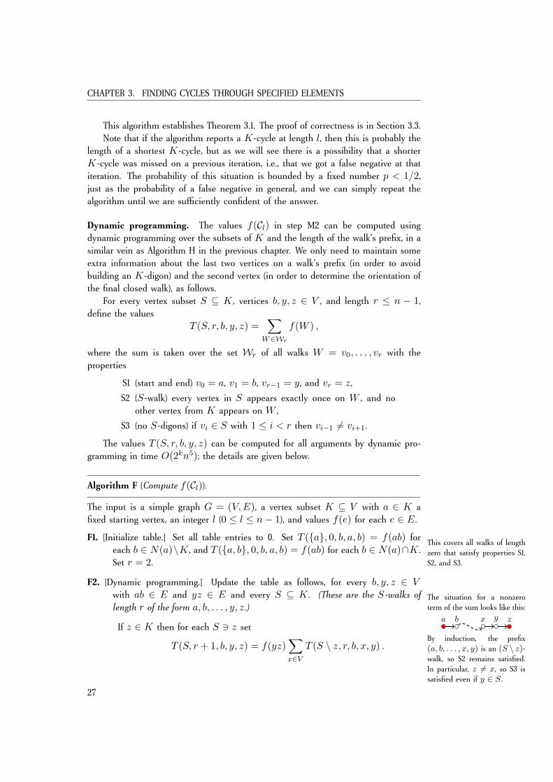
F2. [Dynamic programming.] Update the table as follows, for every b, y, z ∈ Vwith ab ∈ E and yz ∈ E and every S ⊆ K . (These are the S-walks oflength r of the form a, b, . . . , y, z.)
If z ∈ K then for each S 3 z set
T (S, r + 1, b, y, z) = f(yz)∑x∈V
T (S \ z, r, b, x, y) .
The situation for a nonzeroterm of the sum looks like this:
a b x y z
By induction, the prefix(a, b, . . . , x, y) is an (S \ z)-walk, so S2 remains satisfied.In particular, z 6= x, so S3 issatisfied even if y ∈ S.
27
3.2. ALGORITHM
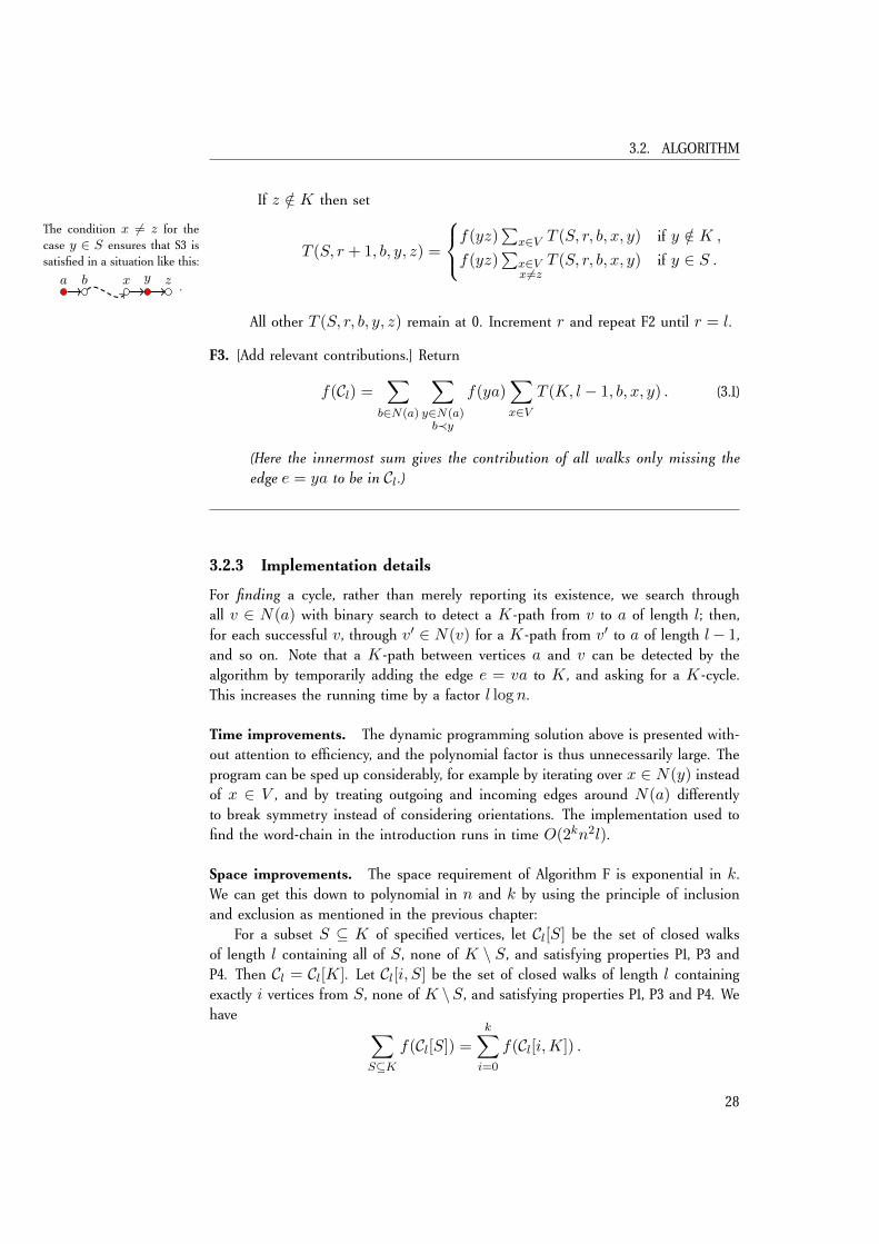
If z /∈ K then set
T (S, r + 1, b, y, z) =
f(yz)∑
x∈V T (S, r, b, x, y) if y /∈ K ,
f(yz)∑
x∈Vx 6=z
T (S, r, b, x, y) if y ∈ S .
The condition x 6= z for thecase y ∈ S ensures that S3 issatisfied in a situation like this:
a b x y z .
All other T (S, r, b, y, z) remain at 0. Increment r and repeat F2 until r = l.
F3. [Add relevant contributions.] Return
f(Cl) =∑
b∈N(a)
∑y∈N(a)b≺y
f(ya)∑x∈V
T (K, l − 1, b, x, y) . (3.1)
(Here the innermost sum gives the contribution of all walks only missing theedge e = ya to be in Cl.)
3.2.3 Implementation details
For finding a cycle, rather than merely reporting its existence, we search throughall v ∈ N(a) with binary search to detect a K-path from v to a of length l; then,for each successful v, through v′ ∈ N(v) for a K-path from v′ to a of length l− 1,and so on. Note that a K-path between vertices a and v can be detected by thealgorithm by temporarily adding the edge e = va to K , and asking for a K-cycle.This increases the running time by a factor l log n.
Time improvements. The dynamic programming solution above is presented with-out attention to efficiency, and the polynomial factor is thus unnecessarily large. Theprogram can be sped up considerably, for example by iterating over x ∈ N(y) insteadof x ∈ V , and by treating outgoing and incoming edges around N(a) differentlyto break symmetry instead of considering orientations. The implementation used tofind the word-chain in the introduction runs in time O(2kn2l).
Space improvements. The space requirement of Algorithm F is exponential in k.We can get this down to polynomial in n and k by using the principle of inclusionand exclusion as mentioned in the previous chapter:
For a subset S ⊆ K of specified vertices, let Cl[S] be the set of closed walksof length l containing all of S , none of K \ S , and satisfying properties P1, P3 andP4. Then Cl = Cl[K]. Let Cl[i, S] be the set of closed walks of length l containingexactly i vertices from S , none of K \S , and satisfying properties P1, P3 and P4. Wehave ∑
S⊆Kf(Cl[S]) =
k∑i=0
f(Cl[i,K]) .
28
CHAPTER 3. FINDING CYCLES THROUGH SPECIFIED ELEMENTS
By the principle of inclusion and exclusion—we here use a different formulation thanthat used for (2.1)—we get
f(Cl[K]) =∑S⊆K
(−1)|K|−|S|k∑i=0
f(Cl[i, S]) .
Thus
f(Cl) =∑S⊆K
k∑i=0
f(Cl[i, S]) mod 2 , (3.2)
and for all S ⊆ K the inner sum in (3.2) can be computed by dynamic programmingin Fq in a similar fashion as Algorithm F above, over the walk’s prefix/suffix, lengthand number of visited K-vertices, rather than over the subsets themselves.
3.3 Correctness
To see that Algorithm M is correct, we use a polynomial-sieving formulation akin tothe one in Section 2.2. We consider the polynomial pl ∈ Fq[x1, . . . , xm] defined fora given graph G = (V,E) and specified subset K ⊆ V by
pl(x1, . . . , xm) =∑W∈Cl
∏ei∈E(W )
xi . (3.3)
Then f(Cl) = pl(f(e1), . . . , f(em)). From the definition, it is clear that pl is apolynomial in m variables of total degree l.
The following result implies correctness of Algorithm M. We let π(l) denote theparity of l.
Lemma 3.1. Let G = (V,E) be a simple graph with K ⊆ V , and let pl ∈Fq[x1, . . . , xm] be defined as in (3.3). If G has no K-cycle of parity π(l) and lengthat most l − 2, then it has a K-cycle of length l if and only if pl is nonzero.
We break this lemma into Lemma 3.2 and Lemma 3.3 below.
Since Algorithm M chooses the values f(e1), . . . , f(em) at random, we canview its behaviour as evaluating pl(x1, . . . , xm) at a random point in Fmq . If pl isidentically zero, then Algorithm M never reports a nonzero value. Conversely, theprobability of a false negative, that is, reporting 0 when pl is not identically zero, isbounded by l/q by the DeMillo-Lipton-Schwartz-Zippel lemma (Lemma 2.1).
We note that if a false negative has been reported at length l, Algorithm M willcontinue to search for longer K-cycles. Then Lemma 3.1 no longer applies for thesesubsequent iterations, and the algorithm may report something nonzero at a higheriteration, regardless of whether there are longer K-cycles or not in the graph. Thus,if the algorithm terminates with pl 6= 0 for some l, we can be completely certain thatthere is a shortest K-cycle of length at most l, but with a probability less than l/qthe shortest K-cycle is actually shorter than l. If there is no K-cycle of the reported
29

3.3. CORRECTNESS
length l in the graph, then this is necessarily discovered during the search step, andwe simply repeat the algorithm until we find a shorter length. Otherwise we find aK-cycle of length l that has a small probability of not being a shortest one of thegiven parity.
It remains to establish Lemma 3.1.
Lemma 3.2. If G has a K-cycle of length l, then pl is nonzero in Fq[x1, . . . , xm].
Proof. A K-cycle C ∈ Cl contributes the monomial
mC =∏
ei∈E(C)
xi
to pl. This monomial depends only on the set of edges on C . With properties P3and P1, the simple cycle C can be recovered from E(C), so mC will be a uniquecontribution to pl and thus constitutes a nonzero term over Fq .
We now argue that all walks in Cl must pair up and cancel whenever G hasno K-cycle of length at most l and of the same parity as l. To show this, wedefine a fixed-point-free involution on Cl, that is, a mapping φ : Cl → Cl suchthat φ(φ(W )) = W and φ(W ) 6= W for all W ∈ Cl. Such a mapping partitions Clinto pairs of walks W,φ(W ).
Lemma 3.3. If G has no K-cycle of parity π(l) and length at most l, then there is afixed-point-free involution φ : Cl → Cl such that f(W ) = f(φ(W )) for each W ∈Cl.
The basic idea of the proof is to define φ like so: Every walk in Cl that isnot a K-cycle must contain a repeated internal vertex. For example, in a graph ofnine vertices labeled 1–9, the closed walk 123567541 contains the repeated internalvertex 5. We want to map this walk to the walk 123
←−−567541 = 123576541 obtained
from reversing the cycle between the first and last occurrence of 5, like this:
1 57→
1 5.
The resulting closed walk is different, yet corresponds to the same monomial since itcontains the same edges. For this idea to work for general closed walks, we need tobe careful about internal palindromes (123
←−−−5676541) and how to choose the repeated
internal vertex.
Proof of Lemma 3.3. We first need some extra terminology. If the end vertex of awalk W and the starting vertex of another walk W ′ are neighbors, we write WW ′
for the concatenated walk. We let←−W denote the reversal of the walk W , and say
that W is a palindrome if W =←−W . A palindrome is nontrivial if it contains more
than one vertex. A repeated internal vertex on a walk is critical. If u is a criticalvertex in W , define
30
CHAPTER 3. FINDING CYCLES THROUGH SPECIFIED ELEMENTS
[uWu] : The subwalk in W of maximum lengthstarting and ending at u.
Given a critical vertex u of W , we can decompose W as
W = X[uWu]Z , (3.4)
for some prefix X and suffix Z of W , such that neither X nor Z contains u. Bycontraction of [uWu] in W we refer to the operation X[uWu]Z 7→ XuZ .
Let G be a graph without K-cycles of parity π(l) and length at most l. Wedefine the mapping φ : Cl → Cl as follows. Given a walk W ∈ Cl, let v be theoutput from the following procedure:
Algorithm R (Find v).
The input is W ∈ Cl.
R1. Let i = 0 and W0 = W .
R2. Let v be the first critical vertex in Wi.
R3. Decompose Wi as X[vWiv]Z . If [vWiv] is a palindrome, set Wi+1 = XvZ ,increment i, and go to R2.
R4. Return v. ([vWiv] is not a palindrome.)
Decompose W as X[vWv]Z for the vertex v returned by Algorithm R, and let
φ : X[vWv]Z 7→ X←−−−−[vWv]Z .
(For example, on input 12345432345467861, Algorithm R returns v = 6:
W0 = 1[2345432]345467861 ,W1 = 123[454]67861 ,W2 = 1234[6786]1 ,
(3.5)
soφ(12345432345467861) = 123454323454
←−−67861
= 12345432345468761 .)
To see that φ is well-defined, we need to show that Algorithm R does outputa critical vertex v on input W ∈ Cl. We first show that Algorithm R satisfies thefollowing invariant:
I1. Wi ∈ Cl−2m for some m ≥ 0 .
31
3.3. CORRECTNESS
The proof is by induction on i, with the case i = 0 established by the inputrequirement. Suppose that Wi−1 ∈ Cl−2m′ for some m′ ≥ 0. Note that Wi isobtained from Wi−1 by contracting some nontrivial palindromic subwalk. Sinceany palindromic walk has even length, the length of Wi must be l − 2m for somem > m′. It remains to check that Wi satisfies properties P1–P4.
Firstly, no nontrivial palindrome [uWi−1u] can contain any specified verticex x ∈K , for as Wi−1 satisfies property P4, x cannot be the middle vertex in [uWi−1u],and as Wi−1 satisfies property P2, x cannot be any of the other vertices of [uWi−1u],because these are necessarily critical. Thus, Wi must contain every vertex in K thatis present in Wi−1, so properties P1 (since a ∈ K ) and P2 will remain satisfiedin Wi. Also P3 remains satisfied, since the given total order of vertices in N(a) isunaffected by contractions. As for property P4, note that if the jth node vj on Wi−1is removed in Wi, then its neighbors vj−1 and vj+1 on Wi−1 must both appearin the palindrome [uWi−1u] that is contracted in Wi, so by the above argumentvj−1, vj+1 /∈ K . This means that neighbors on Wi−1 of any vertex in K must bepreserved in Wi, so no K-digon can appear in Wi as a result of the contraction, andproperty P4 remains satisfied. We conclude that Wi ∈ Cl−2m for some m > m′ ≥ 0.
It follows that Algorithm R must terminate; otherwise, Wi would eventually haveno critical vertex, and by invariant I1 be a K-cycle in G of length l−2m, contrary toassumption. Also, the output vertex v must be critical in the input walk W , becauseV (Wi) ⊆ V (W ).
To see that φ is an involution on Cl, write
W = X[vWv]Z and φ(W ) = X←−−−−[vWv]Z .
We first note that Algorithm R outputs the same vertex v also on input φ(W ). Thisfollows as W and φ(W ) share the same prefix X , so Algorithm R will perform the
same contractions until it reaches v. It then terminates, returning v, since←−−−−[vWv] is
not a palindrome if [vWv] is not a palindrome. Thus
φ(φ(W )) = X←−−−−←−−−−[vWv]Z = W .
To see that φ is fixed-point-free, it suffices to show that [vWv] is not a palin-drome for the output vertex v. It is clear that at some step of Algorithm R, thesubwalk [vWiv] is not a palindrome. The following invariant then provides proof bycontrapositive.
I2. If u is a critical vertex in Wi such that [uWiu] is a palindrome,then [uWi+1u] will also be a palindrome.
We verify I2 by considering cases. Let v be the first critical vertex in Wi. If v = u,then [uWi+1u] = u, a palindrome. If [vWiv] contains no copy of u, or is not a
32
CHAPTER 3. FINDING CYCLES THROUGH SPECIFIED ELEMENTS
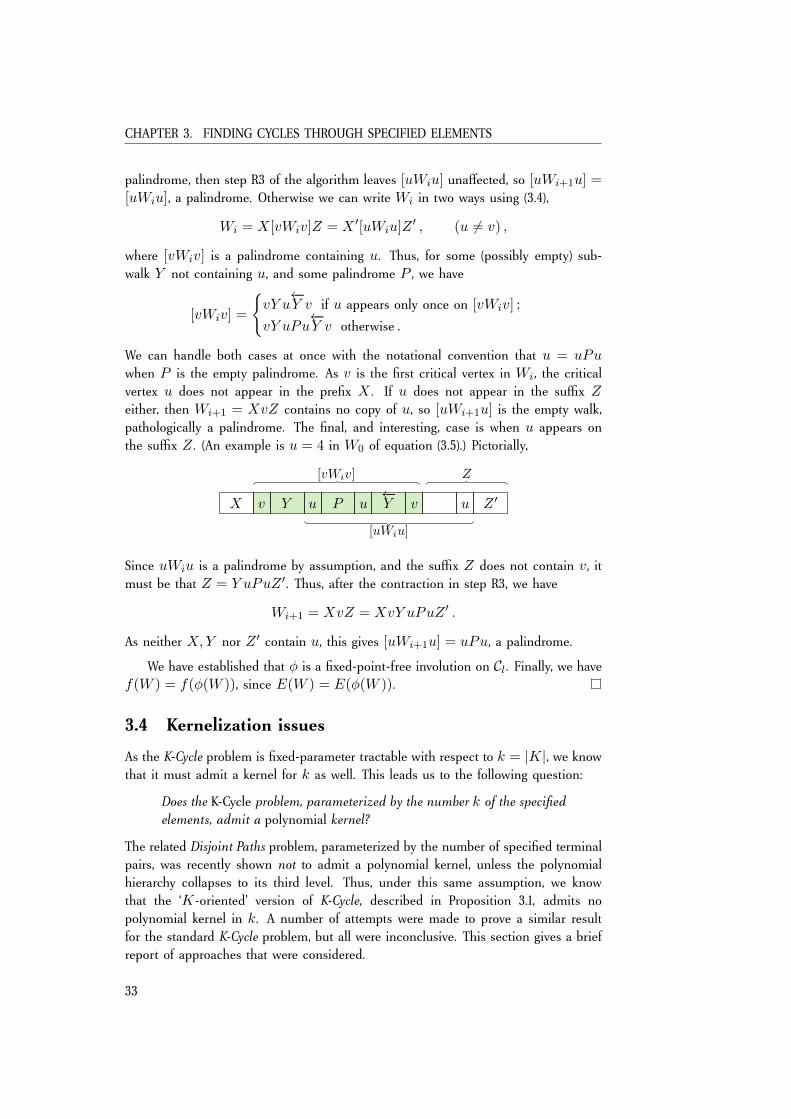
palindrome, then step R3 of the algorithm leaves [uWiu] unaffected, so [uWi+1u] =[uWiu], a palindrome. Otherwise we can write Wi in two ways using (3.4),
Wi = X[vWiv]Z = X ′[uWiu]Z ′ , (u 6= v) ,
where [vWiv] is a palindrome containing u. Thus, for some (possibly empty) sub-walk Y not containing u, and some palindrome P , we have
[vWiv] =
vY u←−Y v if u appears only once on [vWiv] ;
vY uPu←−Y v otherwise .
We can handle both cases at once with the notational convention that u = uPuwhen P is the empty palindrome. As v is the first critical vertex in Wi, the criticalvertex u does not appear in the prefix X . If u does not appear in the suffix Zeither, then Wi+1 = XvZ contains no copy of u, so [uWi+1u] is the empty walk,pathologically a palindrome. The final, and interesting, case is when u appears onthe suffix Z . (An example is u = 4 in W0 of equation (3.5).) Pictorially,
X v Y u P u←−Y v u Z ′
Z[vWiv]
[uWiu]
Since uWiu is a palindrome by assumption, and the suffix Z does not contain v, itmust be that Z = Y uPuZ ′. Thus, after the contraction in step R3, we have
Wi+1 = XvZ = XvY uPuZ ′ .
As neither X,Y nor Z ′ contain u, this gives [uWi+1u] = uPu, a palindrome.
We have established that φ is a fixed-point-free involution on Cl. Finally, we havef(W ) = f(φ(W )), since E(W ) = E(φ(W )).
3.4 Kernelization issues
As the K-Cycle problem is fixed-parameter tractable with respect to k = |K|, we knowthat it must admit a kernel for k as well. This leads us to the following question:
Does the K-Cycle problem, parameterized by the number k of the specifiedelements, admit a polynomial kernel?
The related Disjoint Paths problem, parameterized by the number of specified terminalpairs, was recently shown not to admit a polynomial kernel, unless the polynomialhierarchy collapses to its third level. Thus, under this same assumption, we knowthat the ‘K-oriented’ version of K-Cycle, described in Proposition 3.1, admits nopolynomial kernel in k. A number of attempts were made to prove a similar resultfor the standard K-Cycle problem, but all were inconclusive. This section gives a briefreport of approaches that were considered.
33
3.4. KERNELIZATION ISSUES
Latest developments. We now have an explanation to the failure of the belowdescribed attempts; it has, quite recently, come to the attention of the author thatMagnus Wahlström has found a polynomial kernel for the K-Cycle problem. Thismarks a fundamental difference to the Disjoint Paths problem. The exponential-timeupper bound for the K-Cycle problem remains unchanged, however, as the newly foundkernel does not provide a better exponential dependency on k than the algorithmpresented in this chapter.
3.4.1 Kernelization lower bounds via composition
In [12], Bodlaender et al. initiated the study of superpolynomial lower bounds ofkernel sizes for fixed-parameter tractable problems. To this end they introduced theconcepts of or-composition and and-composition for a parameterized problem.
Definition 3.3. An or-composition for a parameterized problem P is a polynomial-time algorithm with the following behavior:
Input: A number of P-instances (P1, k), . . . , (Pr, k).Task: Find a P-instance (P ′, k′) such that
1. k′ is polynomial in k, and2. (P ′, k′) has a solution⇔ (Pi, ki) has a solution for some i.
An and-composition is defined analogously, with requirement 2. sharpened torequire that (Pi, ki) has a solution for all i ∈ 1, . . . r.
Together with the following theorem, these types of compositionality can be usedto rule out polynomial kernels. The result for or-composition is due to Bodlaenderet al. [12] and Fortnow and Santhanam [38]; the result for and-composition is due toBodlaender et al. [12] and Drucker [33].
Theorem 3.2 (Bodlaender et al. [12], Fortnow and Santhanam [38], Drucker [33]). Let Pbe an NP-complete problem that is fixed-parameter tractable with respect to parameterk, and suppose P is or-compositional, or and-compositional, with respect to k. ThenP admits no polynomial kernel in k, unless the polynomial hierarchy collapses to itsthird level.
Several NP-complete, fixed-parameter tractable problems are known to be or-compositional. This is easily seen for problems such as k-Cycle or k-Path parameter-ized by k, where we can simply consider the disjoint union of the input instances.No such obvious or-composition presents itself for the K-Cycle problem, as e.g. thetotal set of specified elements will be spread out over the input instances.
For other problems the notion of and-composition is more natural. For example,the NP-complete problem of finding a Hamiltonian path with given start and end,parameterized by the width of a given tree-decomposition, is easily seen to be and-compositional by forming a chain of the input graphs, connecting them by theirspecified end nodes [14]. Again, the situation is not immediate for the K-Cycle problem.For example, using some chain-construction in the style of the mentioned examplewould multiply our parameter k = |K| by the number of input graphs.
34
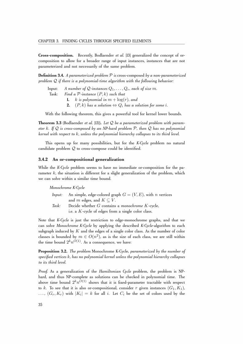
CHAPTER 3. FINDING CYCLES THROUGH SPECIFIED ELEMENTS
Cross-composition. Recently, Bodlaender et al. [13] generalized the concept of or-composition to allow for a broader range of input instances, instances that are notparameterized and not necessarily of the same problem.
Definition 3.4. A parameterized problem P is cross-composed by a non-parameterizedproblem Q if there is a polynomial-time algorithm with the following behavior:
Input: A number of Q-instances Q1, . . . , Qr , each of size m.Task: Find a P-instance (P, k) such that
1. k is polynomial in m+ log(r), and2. (P, k) has a solution⇔ Qi has a solution for some i.
With the following theorem, this gives a powerful tool for kernel lower bounds.
Theorem 3.3 (Bodlaender et al. [13]). Let Q be a parameterized problem with param-eter k. If Q is cross-composed by an NP-hard problem P , then Q has no polynomialkernel with respect to k, unless the polynomial hierarchy collapses to its third level.
This opens up for many possibilities, but for the K-Cycle problem no naturalcandidate problem Q to cross-compose could be identified.
3.4.2 An or-compositional generalization
While the K-Cycle problem seems to have no immediate or-composition for the pa-rameter k, the situation is different for a slight generalization of the problem, whichwe can solve within a similar time bound.
Monochrome K-Cycle
Input: An simple, edge-colored graph G = (V,E), with n verticesand m edges, and K ⊆ V .
Task: Decide whether G contains a monochrome K-cycle,i.e. a K-cycle of edges from a single color class.
Note that K-Cycle is just the restriction to edge-monochrome graphs, and that wecan solve Monochrome K-Cycle by applying the described K-Cycle-algorithm to eachsubgraph induced by K and the edges of a single color class. As the number of colorclasses is bounded by m ∈ O(n2), as is the size of each class, we are still withinthe time bound 2knO(1). As a consequence, we have:
Proposition 3.2. The problem Monochrome K-Cycle, parameterized by the number ofspecified vertices k, has no polynomial kernel unless the polynomial hierarchy collapsesto its third level.
Proof. As a generalization of the Hamiltonian Cycle problem, the problem is NP-hard, and thus NP-complete as solutions can be checked in polynomial time. Theabove time bound 2knO(1) shows that it is fixed-parameter tractable with respectto k. To see that it is also or-compositional, consider r given instances (G1,K1),. . . , (Gr,Kr) with |Ki| = k for all i. Let Ci be the set of colors used by the
35
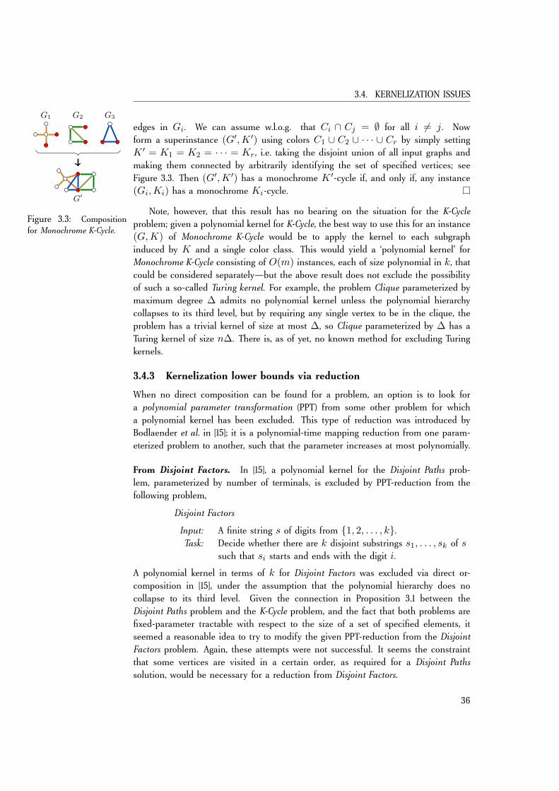
3.4. KERNELIZATION ISSUES
edges in Gi. We can assume w.l.o.g. that Ci ∩ Cj = ∅ for all i 6= j. Nowform a superinstance (G′,K ′) using colors C1 ∪ C2 ∪ · · · ∪ Cr by simply settingK ′ = K1 = K2 = · · · = Kr , i.e. taking the disjoint union of all input graphs andmaking them connected by arbitrarily identifying the set of specified vertices; seeFigure 3.3. Then (G′,K ′) has a monochrome K ′-cycle if, and only if, any instance
G1 G2 G3
G′
Figure 3.3: Compositionfor Monochrome K-Cycle.
(Gi,Ki) has a monochrome Ki-cycle.
Note, however, that this result has no bearing on the situation for the K-Cycleproblem; given a polynomial kernel for K-Cycle, the best way to use this for an instance(G,K) of Monochrome K-Cycle would be to apply the kernel to each subgraphinduced by K and a single color class. This would yield a ‘polynomial kernel’ forMonochrome K-Cycle consisting of O(m) instances, each of size polynomial in k, thatcould be considered separately—but the above result does not exclude the possibilityof such a so-called Turing kernel. For example, the problem Clique parameterized bymaximum degree ∆ admits no polynomial kernel unless the polynomial hierarchycollapses to its third level, but by requiring any single vertex to be in the clique, theproblem has a trivial kernel of size at most ∆, so Clique parameterized by ∆ has aTuring kernel of size n∆. There is, as of yet, no known method for excluding Turingkernels.
3.4.3 Kernelization lower bounds via reduction
When no direct composition can be found for a problem, an option is to look fora polynomial parameter transformation (PPT) from some other problem for whicha polynomial kernel has been excluded. This type of reduction was introduced byBodlaender et al. in [15]; it is a polynomial-time mapping reduction from one param-eterized problem to another, such that the parameter increases at most polynomially.
From Disjoint Factors. In [15], a polynomial kernel for the Disjoint Paths prob-lem, parameterized by number of terminals, is excluded by PPT-reduction from thefollowing problem,
Disjoint Factors
Input: A finite string s of digits from 1, 2, . . . , k.Task: Decide whether there are k disjoint substrings s1, . . . , sk of s
such that si starts and ends with the digit i.
A polynomial kernel in terms of k for Disjoint Factors was excluded via direct or-composition in [15], under the assumption that the polynomial hierarchy does nocollapse to its third level. Given the connection in Proposition 3.1 between theDisjoint Paths problem and the K-Cycle problem, and the fact that both problems arefixed-parameter tractable with respect to the size of a set of specified elements, itseemed a reasonable idea to try to modify the given PPT-reduction from the DisjointFactors problem. Again, these attempts were not successful. It seems the constraintthat some vertices are visited in a certain order, as required for a Disjoint Pathssolution, would be necessary for a reduction from Disjoint Factors.
36
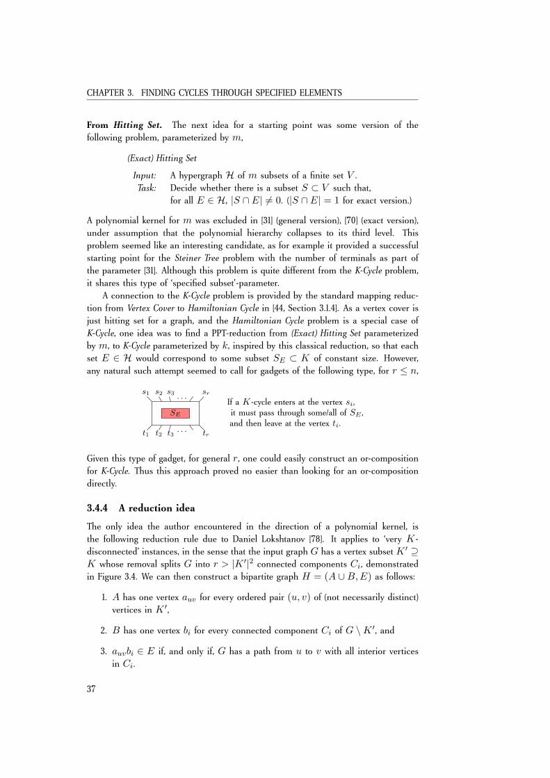
CHAPTER 3. FINDING CYCLES THROUGH SPECIFIED ELEMENTS
From Hitting Set. The next idea for a starting point was some version of thefollowing problem, parameterized by m,
(Exact) Hitting Set
Input: A hypergraph H of m subsets of a finite set V .Task: Decide whether there is a subset S ⊂ V such that,
for all E ∈ H, |S ∩ E| 6= 0. (|S ∩ E| = 1 for exact version.)
A polynomial kernel for m was excluded in [31] (general version), [70] (exact version),under assumption that the polynomial hierarchy collapses to its third level. Thisproblem seemed like an interesting candidate, as for example it provided a successfulstarting point for the Steiner Tree problem with the number of terminals as part ofthe parameter [31]. Although this problem is quite different from the K-Cycle problem,it shares this type of ‘specified subset’-parameter.
A connection to the K-Cycle problem is provided by the standard mapping reduc-tion from Vertex Cover to Hamiltonian Cycle in [44, Section 3.1.4]. As a vertex cover isjust hitting set for a graph, and the Hamiltonian Cycle problem is a special case ofK-Cycle, one idea was to find a PPT-reduction from (Exact) Hitting Set parameterizedby m, to K-Cycle parameterized by k, inspired by this classical reduction, so that eachset E ∈ H would correspond to some subset SE ⊂ K of constant size. However,any natural such attempt seemed to call for gadgets of the following type, for r ≤ n,
SE
s1 s2 s3 sr. . .
t1 t2 t3 tr. . .
If a K-cycle enters at the vertex si,it must pass through some/all of SE ,and then leave at the vertex ti.
Given this type of gadget, for general r, one could easily construct an or-compositionfor K-Cycle. Thus this approach proved no easier than looking for an or-compositiondirectly.
3.4.4 A reduction idea
The only idea the author encountered in the direction of a polynomial kernel, isthe following reduction rule due to Daniel Lokshtanov [78]. It applies to ‘very K-disconnected’ instances, in the sense that the input graph G has a vertex subset K ′ ⊇K whose removal splits G into r > |K ′|2 connected components Ci, demonstratedin Figure 3.4. We can then construct a bipartite graph H = (A ∪B,E) as follows:
1. A has one vertex auv for every ordered pair (u, v) of (not necessarily distinct)vertices in K ′,
2. B has one vertex bi for every connected component Ci of G \K ′, and
3. auvbi ∈ E if, and only if, G has a path from u to v with all interior verticesin Ci.
37
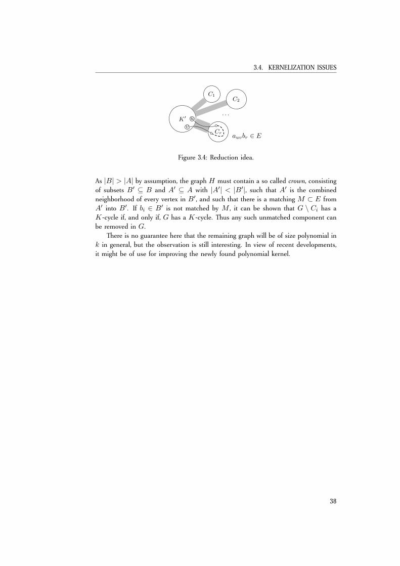
3.4. KERNELIZATION ISSUES
K′
C1C2
Cr
u
v
. . .
auvbr ∈ E
Figure 3.4: Reduction idea.
As |B| > |A| by assumption, the graph H must contain a so called crown, consistingof subsets B′ ⊆ B and A′ ⊆ A with |A′| < |B′|, such that A′ is the combinedneighborhood of every vertex in B′, and such that there is a matching M ⊂ E fromA′ into B′. If bi ∈ B′ is not matched by M , it can be shown that G \ Ci has aK-cycle if, and only if, G has a K-cycle. Thus any such unmatched component canbe removed in G.
There is no guarantee here that the remaining graph will be of size polynomial ink in general, but the observation is still interesting. In view of recent developments,it might be of use for improving the newly found polynomial kernel.
38

Part II
Exponential-Time Complexity inthe Tutte Plane
39

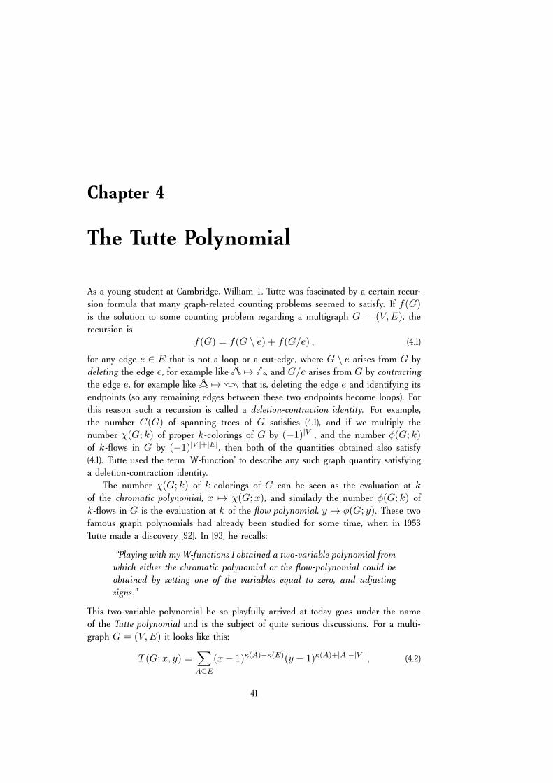
Chapter 4
The Tutte Polynomial
As a young student at Cambridge, William T. Tutte was fascinated by a certain recur-sion formula that many graph-related counting problems seemed to satisfy. If f(G)is the solution to some counting problem regarding a multigraph G = (V,E), therecursion is
f(G) = f(G \ e) + f(G/e) , (4.1)
for any edge e ∈ E that is not a loop or a cut-edge, where G \ e arises from G bydeleting the edge e, for example like 7→ , and G/e arises from G by contractingthe edge e, for example like 7→ , that is, deleting the edge e and identifying itsendpoints (so any remaining edges between these two endpoints become loops). Forthis reason such a recursion is called a deletion-contraction identity. For example,the number C(G) of spanning trees of G satisfies (4.1), and if we multiply thenumber χ(G; k) of proper k-colorings of G by (−1)|V |, and the number φ(G; k)of k-flows in G by (−1)|V |+|E|, then both of the quantities obtained also satisfy(4.1). Tutte used the term ‘W-function’ to describe any such graph quantity satisfyinga deletion-contraction identity.
The number χ(G; k) of k-colorings of G can be seen as the evaluation at kof the chromatic polynomial, x 7→ χ(G;x), and similarly the number φ(G; k) ofk-flows in G is the evaluation at k of the flow polynomial, y 7→ φ(G; y). These twofamous graph polynomials had already been studied for some time, when in 1953Tutte made a discovery [92]. In [93] he recalls:
“Playing with my W-functions I obtained a two-variable polynomial fromwhich either the chromatic polynomial or the flow-polynomial could beobtained by setting one of the variables equal to zero, and adjustingsigns.”
This two-variable polynomial he so playfully arrived at today goes under the nameof the Tutte polynomial and is the subject of quite serious discussions. For a multi-graph G = (V,E) it looks like this:
T (G;x, y) =∑A⊆E
(x− 1)κ(A)−κ(E)(y − 1)κ(A)+|A|−|V | , (4.2)
41
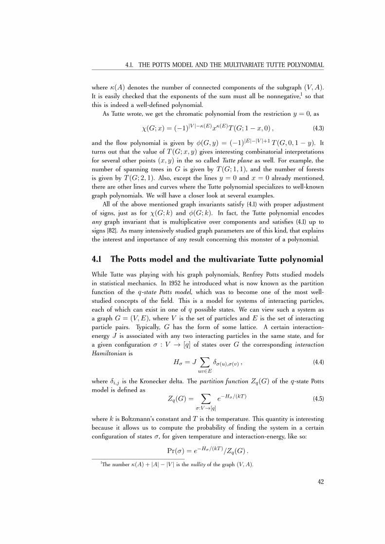
4.1. THE POTTS MODEL AND THE MULTIVARIATE TUTTE POLYNOMIAL
where κ(A) denotes the number of connected components of the subgraph (V,A).It is easily checked that the exponents of the sum must all be nonnegative,1 so thatthis is indeed a well-defined polynomial.
As Tutte wrote, we get the chromatic polynomial from the restriction y = 0, as
χ(G;x) = (−1)|V |−κ(E)xκ(E)T (G; 1− x, 0) , (4.3)
and the flow polynomial is given by φ(G, y) = (−1)|E|−|V |+1 T (G, 0, 1 − y). Itturns out that the value of T (G;x, y) gives interesting combinatorial interpretationsfor several other points (x, y) in the so called Tutte plane as well. For example, thenumber of spanning trees in G is given by T (G; 1, 1), and the number of forestsis given by T (G; 2, 1). Also, except the lines y = 0 and x = 0 already mentioned,there are other lines and curves where the Tutte polynomial specializes to well-knowngraph polynomials. We will have a closer look at several examples.
All of the above mentioned graph invariants satisfy (4.1) with proper adjustmentof signs, just as for χ(G; k) and φ(G; k). In fact, the Tutte polynomial encodesany graph invariant that is multiplicative over components and satisfies (4.1) up tosigns [82]. As many intensively studied graph parameters are of this kind, that explainsthe interest and importance of any result concerning this monster of a polynomial.
4.1 The Potts model and the multivariate Tutte polynomial
While Tutte was playing with his graph polynomials, Renfrey Potts studied modelsin statistical mechanics. In 1952 he introduced what is now known as the partitionfunction of the q-state Potts model, which was to become one of the most well-studied concepts of the field. This is a model for systems of interacting particles,each of which can exist in one of q possible states. We can view such a system asa graph G = (V,E), where V is the set of particles and E is the set of interactingparticle pairs. Typically, G has the form of some lattice. A certain interaction-energy J is associated with any two interacting particles in the same state, and fora given configuration σ : V → [q] of states over G the corresponding interactionHamiltonian is
Hσ = J∑uv∈E
δσ(u),σ(v) , (4.4)
where δi,j is the Kronecker delta. The partition function Zq(G) of the q-state Pottsmodel is defined as
Zq(G) =∑
σ:V→[q]
e−Hσ/(kT ) (4.5)
where k is Boltzmann’s constant and T is the temperature. This quantity is interestingbecause it allows us to compute the probability of finding the system in a certainconfiguration of states σ, for given temperature and interaction-energy, like so:
Pr(σ) = e−Hσ/(kT )/Zq(G) .
1The number κ(A) + |A| − |V | is the nullity of the graph (V,A).
42
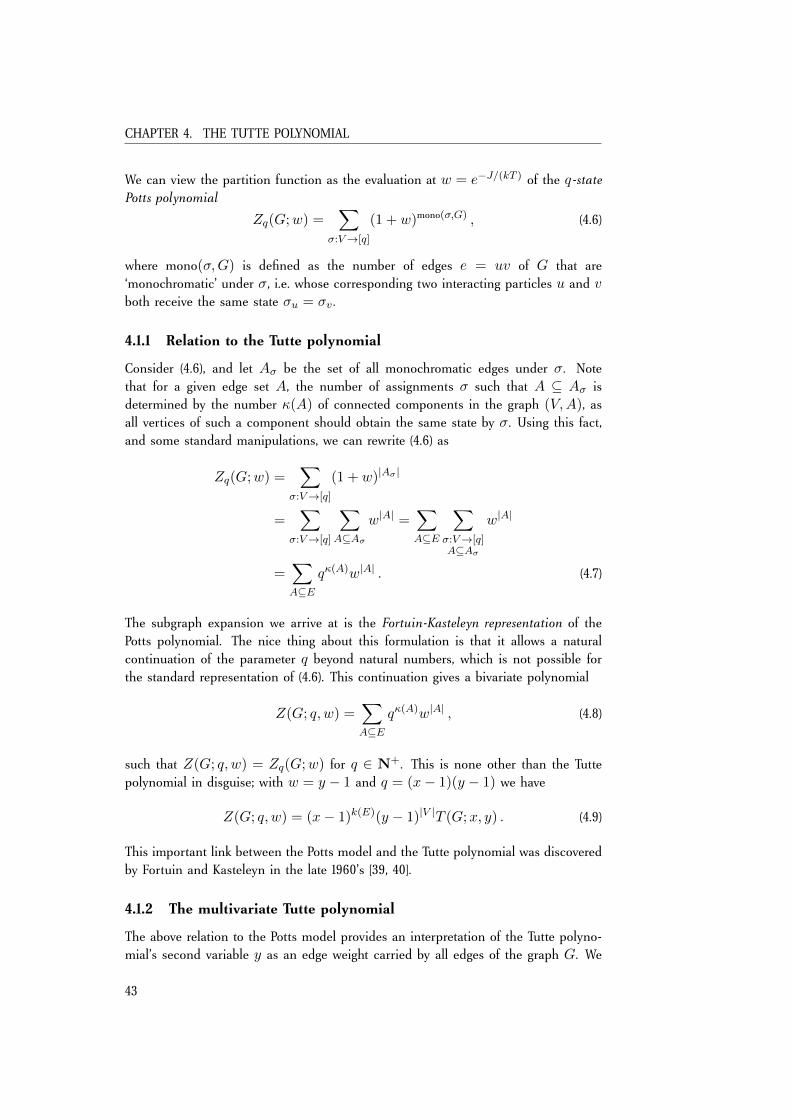
CHAPTER 4. THE TUTTE POLYNOMIAL
We can view the partition function as the evaluation at w = e−J/(kT ) of the q-statePotts polynomial
Zq(G;w) =∑
σ:V→[q]
(1 + w)mono(σ,G) , (4.6)
where mono(σ,G) is defined as the number of edges e = uv of G that are‘monochromatic’ under σ, i.e. whose corresponding two interacting particles u and vboth receive the same state σu = σv .
4.1.1 Relation to the Tutte polynomial
Consider (4.6), and let Aσ be the set of all monochromatic edges under σ. Notethat for a given edge set A, the number of assignments σ such that A ⊆ Aσ isdetermined by the number κ(A) of connected components in the graph (V,A), asall vertices of such a component should obtain the same state by σ. Using this fact,and some standard manipulations, we can rewrite (4.6) as
Zq(G;w) =∑
σ:V→[q]
(1 + w)|Aσ |
=∑
σ:V→[q]
∑A⊆Aσ
w|A| =∑A⊆E
∑σ:V→[q]A⊆Aσ
w|A|
=∑A⊆E
qκ(A)w|A| . (4.7)
The subgraph expansion we arrive at is the Fortuin-Kasteleyn representation of thePotts polynomial. The nice thing about this formulation is that it allows a naturalcontinuation of the parameter q beyond natural numbers, which is not possible forthe standard representation of (4.6). This continuation gives a bivariate polynomial
Z(G; q, w) =∑A⊆E
qκ(A)w|A| , (4.8)
such that Z(G; q, w) = Zq(G;w) for q ∈ N+. This is none other than the Tuttepolynomial in disguise; with w = y − 1 and q = (x− 1)(y − 1) we have
Z(G; q, w) = (x− 1)k(E)(y − 1)|V |T (G;x, y) . (4.9)
This important link between the Potts model and the Tutte polynomial was discoveredby Fortuin and Kasteleyn in the late 1960’s [39, 40].
4.1.2 The multivariate Tutte polynomial
The above relation to the Potts model provides an interpretation of the Tutte polyno-mial’s second variable y as an edge weight carried by all edges of the graph G. We
43
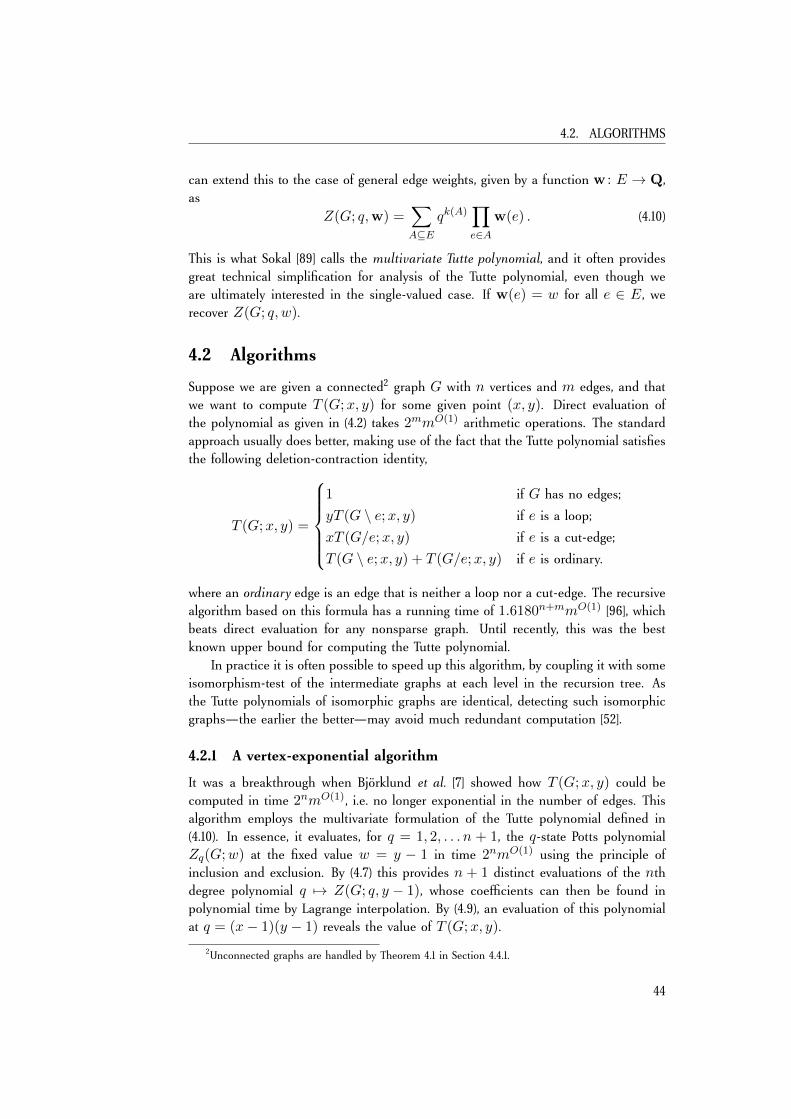
4.2. ALGORITHMS
can extend this to the case of general edge weights, given by a function w : E → Q,as
Z(G; q,w) =∑A⊆E
qk(A)∏e∈A
w(e) . (4.10)
This is what Sokal [89] calls the multivariate Tutte polynomial, and it often providesgreat technical simplification for analysis of the Tutte polynomial, even though weare ultimately interested in the single-valued case. If w(e) = w for all e ∈ E , werecover Z(G; q, w).
4.2 Algorithms
Suppose we are given a connected2 graph G with n vertices and m edges, and thatwe want to compute T (G;x, y) for some given point (x, y). Direct evaluation ofthe polynomial as given in (4.2) takes 2mmO(1) arithmetic operations. The standardapproach usually does better, making use of the fact that the Tutte polynomial satisfiesthe following deletion-contraction identity,
T (G;x, y) =
1 if G has no edges;
yT (G \ e;x, y) if e is a loop;
xT (G/e;x, y) if e is a cut-edge;
T (G \ e;x, y) + T (G/e;x, y) if e is ordinary.
where an ordinary edge is an edge that is neither a loop nor a cut-edge. The recursivealgorithm based on this formula has a running time of 1.6180n+mmO(1) [96], whichbeats direct evaluation for any nonsparse graph. Until recently, this was the bestknown upper bound for computing the Tutte polynomial.
In practice it is often possible to speed up this algorithm, by coupling it with someisomorphism-test of the intermediate graphs at each level in the recursion tree. Asthe Tutte polynomials of isomorphic graphs are identical, detecting such isomorphicgraphs—the earlier the better—may avoid much redundant computation [52].
4.2.1 A vertex-exponential algorithm
It was a breakthrough when Björklund et al. [7] showed how T (G;x, y) could becomputed in time 2nmO(1), i.e. no longer exponential in the number of edges. Thisalgorithm employs the multivariate formulation of the Tutte polynomial defined in(4.10). In essence, it evaluates, for q = 1, 2, . . . n + 1, the q-state Potts polynomialZq(G;w) at the fixed value w = y − 1 in time 2nmO(1) using the principle ofinclusion and exclusion. By (4.7) this provides n + 1 distinct evaluations of the nthdegree polynomial q 7→ Z(G; q, y − 1), whose coefficients can then be found inpolynomial time by Lagrange interpolation. By (4.9), an evaluation of this polynomialat q = (x− 1)(y − 1) reveals the value of T (G;x, y).
2Unconnected graphs are handled by Theorem 4.1 in Section 4.4.1.
44
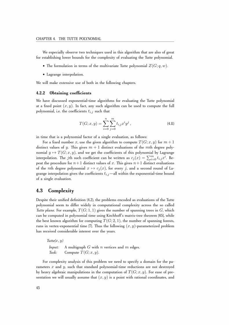
CHAPTER 4. THE TUTTE POLYNOMIAL
We especially observe two techniques used in this algorithm that are also of greatfor establishing lower bounds for the complexity of evaluating the Tutte polynomial.
• The formulation in terms of the multivariate Tutte polynomial Z(G; q, w).
• Lagrange interpolation.
We will make extensive use of both in the following chapters.
4.2.2 Obtaining coefficients
We have discussed exponential-time algorithms for evaluating the Tutte polynomialat a fixed point (x, y). In fact, any such algorithm can be used to compute the fullpolynomial, i.e. the coefficients ti,j such that
T (G;x, y) =n∑i=0
m∑j=0
ti,jxiyj , (4.11)
in time that is a polynomial factor of a single evaluation, as follows:For a fixed number x, use the given algorithm to compute T (G;x, y) for m+ 1
distinct values of y. This gives m + 1 distinct evaluations of the mth degree poly-nomial y 7→ T (G;x, y), and we get the coefficients of this polynomial by Lagrangeinterpolation. The jth such coefficient can be written as cj(x) =
∑mi=0 ti,jx
i. Re-peat the procedure for n+1 distinct values of x. This gives n+1 distinct evaluationsof the nth degree polynomial x 7→ cj(x), for every j, and a second round of La-grange interpolation gives the coefficients ti,j—all within the exponential-time boundof a single evaluation.
4.3 Complexity
Despite their unified definition (4.2), the problems encoded as evaluations of the Tuttepolynomial seem to differ widely in computational complexity across the so calledTutte plane. For example, T (G; 1, 1) gives the number of spanning trees in G, whichcan be computed in polynomial time using Kirchhoff’s matrix-tree theorem [65], whilethe best known algorithm for computing T (G; 2, 1), the number of spanning forests,runs in vertex-exponential time [7]. Thus the following (x, y)-parameterized problemhas received considerable interest over the years.
Tutte(x, y)
Input: A multigraph G with n vertices and m edges.Task: Compute T (G;x, y).
For complexity analysis of this problem we need to specify a domain for the pa-rameters x and y, such that standard polynomial-time reductions are not destroyedby heavy algebraic manipulations in the computation of T (G;x, y). For ease of pre-sentation we will usually assume that (x, y) is a point with rational coordinates, and
45
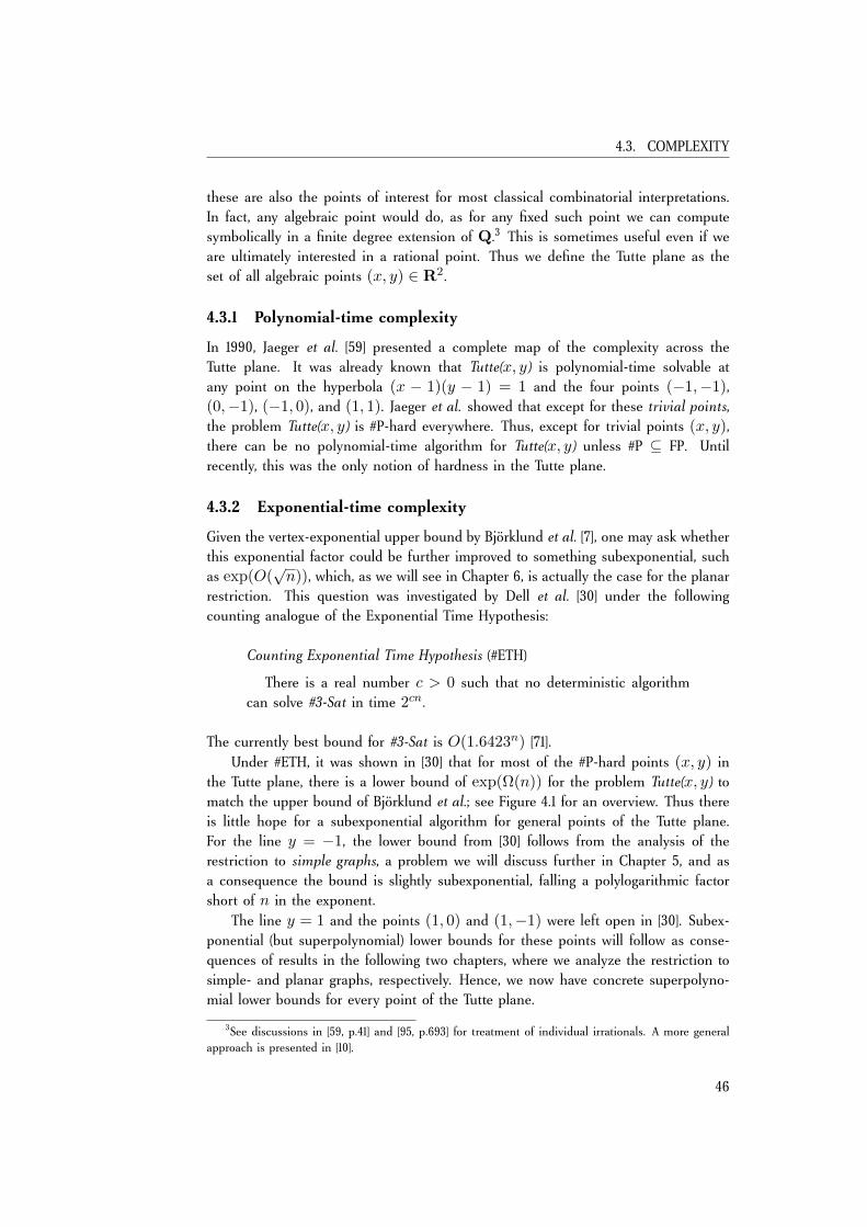
4.3. COMPLEXITY
these are also the points of interest for most classical combinatorial interpretations.In fact, any algebraic point would do, as for any fixed such point we can computesymbolically in a finite degree extension of Q.3 This is sometimes useful even if weare ultimately interested in a rational point. Thus we define the Tutte plane as theset of all algebraic points (x, y) ∈ R2.
4.3.1 Polynomial-time complexity
In 1990, Jaeger et al. [59] presented a complete map of the complexity across theTutte plane. It was already known that Tutte(x, y) is polynomial-time solvable atany point on the hyperbola (x − 1)(y − 1) = 1 and the four points (−1,−1),(0,−1), (−1, 0), and (1, 1). Jaeger et al. showed that except for these trivial points,the problem Tutte(x, y) is #P-hard everywhere. Thus, except for trivial points (x, y),there can be no polynomial-time algorithm for Tutte(x, y) unless #P ⊆ FP. Untilrecently, this was the only notion of hardness in the Tutte plane.
4.3.2 Exponential-time complexity
Given the vertex-exponential upper bound by Björklund et al. [7], one may ask whetherthis exponential factor could be further improved to something subexponential, suchas exp(O(
√n)), which, as we will see in Chapter 6, is actually the case for the planar
restriction. This question was investigated by Dell et al. [30] under the followingcounting analogue of the Exponential Time Hypothesis:
Counting Exponential Time Hypothesis (#ETH)
There is a real number c > 0 such that no deterministic algorithmcan solve #3-Sat in time 2cn.
The currently best bound for #3-Sat is O(1.6423n) [71].Under #ETH, it was shown in [30] that for most of the #P-hard points (x, y) in
the Tutte plane, there is a lower bound of exp(Ω(n)) for the problem Tutte(x, y) tomatch the upper bound of Björklund et al.; see Figure 4.1 for an overview. Thus thereis little hope for a subexponential algorithm for general points of the Tutte plane.For the line y = −1, the lower bound from [30] follows from the analysis of therestriction to simple graphs, a problem we will discuss further in Chapter 5, and asa consequence the bound is slightly subexponential, falling a polylogarithmic factorshort of n in the exponent.
The line y = 1 and the points (1, 0) and (1,−1) were left open in [30]. Subex-ponential (but superpolynomial) lower bounds for these points will follow as conse-quences of results in the following two chapters, where we analyze the restriction tosimple- and planar graphs, respectively. Hence, we now have concrete superpolyno-mial lower bounds for every point of the Tutte plane.
3See discussions in [59, p.41] and [95, p.693] for treatment of individual irrationals. A more generalapproach is presented in [10].
46
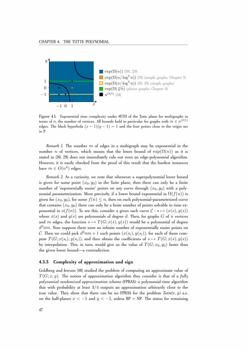
CHAPTER 4. THE TUTTE POLYNOMIAL
x−1 0 1
y
−1
0
1
exp(Ω(n)) [30], [29]
exp(Ω(n/ log2 n)) [29] (simple graphs, Chapter 5)
exp(Ω(n/ log3 n)) [30, 29] (simple graphs)exp(Ω( 8
√n) (planar graphs, Chapter 6)
nO(1) [59]
Figure 4.1: Exponential time complexity under #ETH of the Tutte plane for multigraphs interms of n, the number of vertices. All bounds hold in particular for graphs with m ∈ nO(1)
edges. The black hyperbola (x − 1)(y − 1) = 1 and the four points close to the origin arein P.
Remark 1. The number m of edges in a multigraph may be exponential in thenumber n of vertices, which means that the lower bound of exp(Ω(n)) as it isstated in [30, 29] does not immediately rule out even an edge-polynomial algorithm.However, it is easily checked from the proof of this result that the hardest instanceshave m ∈ O(n4) edges.
Remark 2. As a curiosity, we note that whenever a superpolynomial lower boundis given for some point (x0, y0) in the Tutte plane, then there can only be a finitenumber of ‘exponentially easier’ points on any curve through (x0, y0) with a poly-nomial parameterization. More precisely, if a lower bound exponential in Ω(f(n)) isgiven for (x0, y0), for some f(n) ≤ n, then on each polynomial-parameterized curvethat contains (x0, y0) there can only be a finite number of points solvable in time ex-ponential in o(f(n)). To see this, consider a given such curve C : s 7→ (x(s), y(s))where x(s) and y(s) are polynomials of degree d. Then, for graphs G of n verticesand m edges, the function s 7→ T (G;x(s), y(s)) would be a polynomial of degreed2nm. Now suppose there were an infinite number of exponentially easier points onC. Then we could pick d2nm+ 1 such points (x(si), y(si)), for each of them com-pute T (G;x(si), y(si)), and then obtain the coefficients of s 7→ T (G;x(s), y(s))by interpolation. This, in turn, would give us the value of T (G;x0, y0) faster thanthe given lower bound—a contradiction.
4.3.3 Complexity of approximation and sign
Goldberg and Jerrum [48] studied the problem of computing an approximate value ofT (G;x, y). The notion of approximation algorithm they consider is that of a fullypolynomial randomized approximation scheme (FPRAS): a polynomial-time algorithmthat with probability at least 3/4 outputs an approximation arbitrarily close to thetrue value. They show that there can be no FPRAS for the problem Tutte(x, y) a.e.on the half-planes x < −1 and y < −1, unless RP = NP. The status for remaining
47
4.4. SOME USEFUL PROPERTIES
points with x, y > −1 remains open, except at the known trivial points and theupper branch of the hyperbola (x − 1)(x − 2) = 2, for which a FPRAS followsfrom [60].
Very recently, these results were sharpened as a result of Goldberg and Jerrum’swork on the complexity of computing the sign of T (G;x, y). This seems ‘almost likea decision problem’, as there are only three possible outcomes: positive, negative, orzero, but in [50] they show that, for large regions of the plane, this problem is in fact#P-hard. As a consequence, approximation at these points is also #P-hard. Thus, interms of polynomial-time complexity, approximation is as hard as exact computationfor large parts of the Tutte plane. For most remaining points, including all those withx, y > −1 and x+ y > 0, it is shown that the sign can be computed in polynomialtime, and that an approximation can be computed in polynomial time using an NPoracle. This marks a clear distinction between these problems and exact computationof Tutte(x, y), where we have #P-hardness a.e.
4.3.4 The line y = 1
The line y = 1 in the Tutte plane deserves some attention, because, as Figure 4.1shows, the current lower bound under #ETH for these points is ‘very sub-exponential’.Here the Tutte polynomial specializes to the generating function of forests in G,weighted by the number of edges it contains,
F (G;w) =∑F⊆E
(V,F ) forest
w|F | . (4.12)
The relation to the Tutte polynomial is F (G;w) = w|V |−κ(E)T (G; 1 + 1/w, 1).This line resist the analysis of [48, 50, 30, 29], and, unlike all other nontrivial
points of the Tutte plane, the only proof of #P-hardness at these points relies on the#P-hardness for the restricted class of planar graphs, for which there is a direct proofby Vertigan [95]. As the problem Tutte(x, y) restricted to planar graphs has a knownupper bound exponential in O(
√n) [87], this approach could at best give a lower
bound exponential in Ω(√n) under #ETH. However, not even such a result has been
found for this line.In Chapter 6 we note that the planar reduction of [95] yields a lower bound
exponential in Ω( 8√n) under #ETH for planar multigraphs. This is by reduction
from the problem of computing the coefficients of w 7→ F (G;w), which has thesame lower bound under #ETH. The same reduction can be used directly for generalmultigraphs, but there is no immediate gain in this approach, as no better bound forfinding coefficients of w 7→ F (G;w) for general multigraphs has yet been found.
4.4 Some useful properties
We here list some elementary properties of the Tutte polynomial that will be usefulin the following chapters.
48
CHAPTER 4. THE TUTTE POLYNOMIAL
4.4.1 Deletion-contraction and connectedness
The deletion-contraction identity in (4.13) is sometimes taken as the definition of theTutte polynomial. We restate it here for easy reference.
T (G;x, y) =
1 if G has no edges;
yT (G \ e;x, y) if e is a loop;
xT (G/e;x, y) if e is a cut-edge;
T (G \ e;x, y) + T (G/e;x, y) if e is ordinary.
(4.13)
This formula can be obtained by routine calculations from the subgraph expansion(4.2), considering the effects of a deletion or contraction on the number of compo-nents, vertices, and edges, depending on the type of edge that is manipulated.
The subgraph expansion for the multivariate Tutte polynomial in (4.10) has a lesscomplicated dependency on the number of components than that of the standardTutte polynomial, and the resulting deletion-contraction identity takes the same formregardless of the type of edge under consideration. It follows easily from (4.10) that
Z(G; q,w) = Z(G \ e; q,w) + w(e)Z(G/e; q,w) . (4.14)
Using (4.13), it follows by induction on the number of ordinary edges that theTutte polynomial is multiplicative over 2-connected components:
Theorem 4.1. Let G be the union of two graphs G1 and G2 with at most one vertexin common. Then
T (G;x, y) = T (G1;x, y) · T (G2;x, y) . (4.15)
This means that for exponential-time analysis of Tutte(x, y), we can always assumethat the input graph is 2-connected without loops.
4.4.2 Point shifts, thickenings and stretches
Given two points (x, y) and (x′, y′) in the Tutte plane, there are always some graphsG′ and G such that T (G′;x, y) = T (G;x′, y′). For example,
T ( ;x, y) = T ( ; 0, x3) = x3 .
Sometimes it is possible to define a mapping ϕ, such that for any graph G
T (ϕ(G);x, y) ∼ T (G;x′, y′) ,
where ∼ denotes equality up to some simple closed-form expression. We then saythat the point (x, y) is shifted to the point (x′, y′) via the transformation ϕ. Such ashift provides a reduction from Tutte(x′, y′) to Tutte(x, y). This was one of the maintechniques used by Jaeger et al. in [59] for studying #P-hardness across the Tutte plane,and it is also a crucial tool in the analysis of exponential-time complexity. Note thatthe strength of such a reduction depends on the size of ϕ(G). If, for example,the number of nodes increases quadratically, then a lower bound of exp(Ω(n)) forTutte(x, y) only implies a lower bound of exp(Ω(
√n)) for Tutte(x′, y′).
49
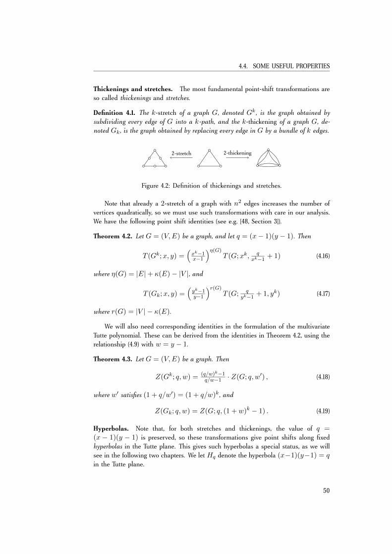
4.4. SOME USEFUL PROPERTIES
Thickenings and stretches. The most fundamental point-shift transformations areso called thickenings and stretches.
Definition 4.1. The k-stretch of a graph G, denoted Gk , is the graph obtained bysubdividing every edge of G into a k-path, and the k-thickening of a graph G, de-noted Gk , is the graph obtained by replacing every edge in G by a bundle of k edges.
2-stretch 2-thickening
Figure 4.2: Definition of thickenings and stretches.
Note that already a 2-stretch of a graph with n2 edges increases the number ofvertices quadratically, so we must use such transformations with care in our analysis.We have the following point shift identities (see e.g. [48, Section 3]).
Theorem 4.2. Let G = (V,E) be a graph, and let q = (x− 1)(y − 1). Then
T (Gk;x, y) =(xk−1x−1
)η(G)T (G;xk, q
xk−1 + 1) (4.16)
where η(G) = |E|+ κ(E)− |V |, and
T (Gk;x, y) =(yk−1y−1
)r(G)T (G; q
yk−1 + 1, yk) (4.17)
where r(G) = |V | − κ(E).
We will also need corresponding identities in the formulation of the multivariateTutte polynomial. These can be derived from the identities in Theorem 4.2, using therelationship (4.9) with w = y − 1.
Theorem 4.3. Let G = (V,E) be a graph. Then
Z(Gk; q, w) = (q/w)k−1q/w−1 · Z(G; q, w′) , (4.18)
where w′ satisfies (1 + q/w′) = (1 + q/w)k , and
Z(Gk; q, w) = Z(G; q, (1 + w)k − 1) . (4.19)
Hyperbolas. Note that, for both stretches and thickenings, the value of q =(x − 1)(y − 1) is preserved, so these transformations give point shifts along fixedhyperbolas in the Tutte plane. This gives such hyperbolas a special status, as we willsee in the following two chapters. We let Hq denote the hyperbola (x−1)(y−1) = qin the Tutte plane.
50
Chapter 5
Lower Bounds for Simple Graphs
In this chapter we consider the restriction of Tutte(x, y) to simple input graphs.
Simple Tutte(x, y)
Input: A simple graph G with n vertices and m edges.Task: Compute T (G;x, y).
This restriction is of particular interest because most of the graphs studied in sta-tistical mechanics arise from bond structures that are simple. From the perspectiveof polynomial-time complexity, the picture of the Tutte plane for simple graphs co-incides with the general case, i.e. Simple Tutte(x, y) is #P-hard for all points (x, y)except for the hyperbola H1 and the points (−1,−1), (0,−1), (−1, 0), and (1, 1),where it is polynomial-time solvable. The study of exponential-time complexity under#ETH was initiated by Dell et al. in [30], where lower bounds exponential in n weregiven for the line y = 0, and exponential in m/ log3(m) for most other points ofthe Tutte plane. These exponential bounds in terms of edge size, together with theknown 2nmO(1)-time upper bound, show that the hardest instances for such pointsare sparse graphs.
A few lines were left open in [30], in particular the line x = 1 which requiresa somewhat different treatment and will be the focus of this chapter. This so calledreliability line was the subject of [56], which is joint work with Thore Husfeldt andcontains a lower bound exponential in m/ log2(m) for all points of the line withy > 1. Together with Holger Dell, the result was extended to the full line x = 1.This work is incorporated into the journal paper [29], which now gives exponential (atleast within a polylogarithmic factor) lower bounds under #ETH for the whole Tutteplane, except the line y = 1; see Figure 5.1 for an overview.
5.1 The reliability polynomial
On the line x = 1, the Tutte polynomial specializes to the reliability polynomial,an object studied in algebraic graph theory [47, Section 15.8]. For a connected
51
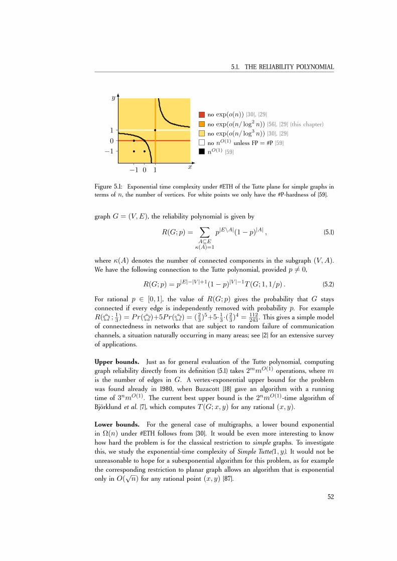
5.1. THE RELIABILITY POLYNOMIAL
x−1 0 1
y
−1
0
1
no exp(o(n)) [30], [29]
no exp(o(n/ log2 n)) [56], [29] (this chapter)
no exp(o(n/ log3 n)) [30], [29]
no nO(1) unless FP = #P [59]
nO(1) [59]
Figure 5.1: Exponential time complexity under #ETH of the Tutte plane for simple graphs interms of n, the number of vertices. For white points we only have the #P-hardness of [59].
graph G = (V,E), the reliability polynomial is given by
R(G; p) =∑A⊆Eκ(A)=1
p|E\A|(1− p)|A| , (5.1)
where κ(A) denotes the number of connected components in the subgraph (V,A).We have the following connection to the Tutte polynomial, provided p 6= 0,
R(G; p) = p|E|−|V |+1(1− p)|V |−1T (G; 1, 1/p) . (5.2)
For rational p ∈ [0, 1], the value of R(G; p) gives the probability that G staysconnected if every edge is independently removed with probability p. For exampleR( ; 1
3) = Pr( )+5Pr( ) = (23)5+5· 13 ·(23)4 = 112
243 . This gives a simple modelof connectedness in networks that are subject to random failure of communicationchannels, a situation naturally occurring in many areas; see [2] for an extensive surveyof applications.
Upper bounds. Just as for general evaluation of the Tutte polynomial, computinggraph reliability directly from its definition (5.1) takes 2mmO(1) operations, where mis the number of edges in G. A vertex-exponential upper bound for the problemwas found already in 1980, when Buzacott [18] gave an algorithm with a runningtime of 3nmO(1). The current best upper bound is the 2nmO(1)-time algorithm ofBjörklund et al. [7], which computes T (G;x, y) for any rational (x, y).
Lower bounds. For the general case of multigraphs, a lower bound exponentialin Ω(n) under #ETH follows from [30]. It would be even more interesting to knowhow hard the problem is for the classical restriction to simple graphs. To investigatethis, we study the exponential-time complexity of Simple Tutte(1, y). It would not beunreasonable to hope for a subexponential algorithm for this problem, as for examplethe corresponding restriction to planar graph allows an algorithm that is exponentialonly in O(
√n) for any rational point (x, y) [87].
52
CHAPTER 5. LOWER BOUNDS FOR SIMPLE GRAPHS
We have R(G; 0) = 1 and R(G; 1) = 0 for all connected graphs, so for p = 0and p = 1 the reliability polynomial is always easy to evaluate. One may askwhat the situation is for values close to these two extremes. Note that p = 1corresponds to the limit point (1, 1) in the Tutte plane, which we know is alsoa polynomial-time point for the problem Tutte(x, y), though for less trivial reasons(Kirchhoff’s matrix-tree theorem). Moreover, for p = 1
2 it is easily seen that (5.1)equals the number of connected, spanning subgraphs of G, divided by 2m. This isan interesting enumeration problem in itself, and one could be tempted to hope foran algorithm faster than vertex-exponential, considering that the related problem offinding the number of spanning trees of G can be solved in polynomial time (again,the point (1, 1) in the Tutte plane).
5.1.1 Main theorem
We give a lower bound of the problem of computing all-terminal graph reliability forthe class of simple graphs for all nontrivial probabilities p. Beyond this interpretation,the lower bound extends to all nontrivial points on the full line x = 1 in theTutte plane. We use the framework introduced by Dell et al. in [30] for studyingexponential-time complexity in the Tutte plane under the hypothesis #ETH.
Theorem 5.1. Let y 6= 1 be a rational number. Then, under #ETH, there is noexp(o(m/ log2m))-time algorithm for Simple Tutte(1, y).
In particular, the bound holds for y = 2, i.e. counting the number of connectedspanning subgraphs of a given graph.
We have expressed the lower bound in terms of the parameter m, the numberof edges of the input graph. Since n ≤ m + 1 for connected graphs, the resultimplies a lower bound of exp(Ω(n/ log2 n)) also in terms of the parameter n,the number of vertices of the input graph. The formulation in terms of m is in-teresting, because together with the vertex-exponential algorithm from [7] it showsthat the hardest instances have roughly linear density, ruling out a better algorithmthan exp(O(n/ log2 n)) even for the restricted case of sparse graphs.
Our bound does not quite match the upper bounds of [18, 7]. This situation issimilar to the bounds reported in [30] for other regions of the Tutte plane, which alsofall a few logarithmic factors (in the exponent) short of the best known algorithms.The bound does, however, suffice to separate the complexity of reliability computationfor simple graphs from the subexponential-time bound for the planar case.
5.1.2 Related work
The structural complexity (in terms of #P-hardness) of Simple Tutte(1, y) follows fromthe mentioned result of Jaeger et al. [59], which covered every point in the Tutteplane, but in fact the case of all-terminal graph reliability was settled by Provanand Ball already in the 1980’s [84]. The reductions in these papers do not preservethe parameters n and m, so that the running time bounds under #ETH implicitlyprovided by their techniques are typically exponential in Ω(n1/k) for some k.
53

5.2. TOOLS ADJUSTED FOR THE RELIABILITY LINE
The problem Simple Tutte(1, y) has a number of natural extensions.
1. We can consider the computational problem of finding the reliability polyno-mial itself, instead of its value at a fixed point p = 1/y. The input to thisproblem is a graph, and the output is a list of coefficients. For example, oninput , the output should be R( ; p) = 4p5 − 15p4 + 20p3 − 10p2 + 1.
2. We can associate individual probabilities to every edge. For example, the graph12
14 becomes disconnected with probability 5
8 .
3. We can consider multigraphs like , but with the same edge-failure prob-ability p. As indicated by the example (set p = 1
2 and compare to the above),the multigraph case is a special case of the individually edge-weighted case, afact that we will use later.
All of these problems are at least as hard as the problem under consideration in thischapter. Lower bounds of size exp(Ω(m)) are given in [30] or follow relatively easily;see Section 5.3.
A recent paper of Hoffman [54] studies the complexity of another graph polyno-mial, the independent set polynomial, in the same framework.
5.2 Tools adjusted for the reliability line
The line x = 1 in the Tutte plane is the vertical component of the hyperbola
H0 = (x, y) : (x− 1)(y − 1) = 0 .
This hyperbola resists the analysis of e.g. [30], because the the multivariate formulationtypically assumes that q = (x − 1)(y − 1) 6= 0. Thus we will need some modifiedversions of the tools described in Chapter 4.
By the multiplicative property (4.15), we can restrict our attention to connectedgraphs G = (V,E), i.e. we may assume that κ(E) = 1 as in the definition of thereliability polynomial.
5.2.1 Multivariate formulation
The multivariate Tutte polynomial Z(G; q,w) defined in (4.10) evaluates to zerowhenever q = 0, which is not very helpful. Instead we consider the following slightlymodified polynomial introduced in Sokal [89, Section 2.3],
Z0(G; q,w) = q−κ(E)Z(G; q,w)
=∑A⊆E
∏e∈A
w(e)qκ(A)−κ(E) . (5.3)
For κ(E) = 1 and q = 0 this gives a weighted version of the reliability polynomial,
R(G;w) =∑A⊆Eκ(A)=1
∏e∈A
w(e) . (5.4)
54

CHAPTER 5. LOWER BOUNDS FOR SIMPLE GRAPHS
We get the following connection to the reliability polynomial, for p 6= 0,
R(G; p) = p|E|R(G; 1p − 1) . (5.5)
5.2.2 Deletion-contraction identity
A deletion-contraction identity for Z0 follows implicitly from (4.14). Since Z0 =q−k(E)Z , equation (4.14) gives
Z0(G; q,w) =
qZ0(G− e; q,w) + w(e)Z0(G/e; q,w) if e is a cut-edge,
Z0(G− e; q,w) + w(e)Z0(G/e; q,w) otherwise.(5.6)
5.2.3 Stretches and thickenings
Along the reliability line, the weight shift identities of Theorem 4.2 for stretches andthickenings are not valid. Goldberg and Jerrum derived corresponding versions for thepolynomial R(G;w) in [48] for the special case when every edge of the inserted k-path or k-bundle has the same weight. We need multiweighted versions of these.By w[e 7→ w′] we denote the function w′ : E(G)→ Q that is identical to w exceptat the edge e where w′(e) = w′.
Lemma 5.1. Let G be a connected graph with edge weights given by w : E(G)→ Q.
(i) If ϕ(G) is obtained from G by replacing a single edge e ∈ E with a simple pathof k edges P = e1, ..., ek with w(ei) = wi, then
R(ϕ(G);w) = CP · R(G;w[e 7→ w′]) ,
where1
w′=
1
w1+ · · ·+ 1
wkand CP =
1
w′
k∏i=1
wi . (5.7)
(ii) If ϕ(G) is obtained from G by replacing a single edge e ∈ E with a bundle of kparallel edges B = e1, . . . , ek with w(ei) = wi, then
R(ϕ(G);w) = R(G;w[e 7→ w′]) ,
where
w′ = −1 +
k∏i=1
(1 + wi) . (5.8)
Proof. We repeat the arguments from the proof in [48, Section 4.3]. For a given setA ⊂ E of edges we let w(P ) =
∏e∈Aw(e).
Let S be the set of subsets A ⊆ E \e that already span the whole graph G =(V,E), i.e.
S = A ⊆ E \ e : κ(A) = 1 ,
55
5.2. TOOLS ADJUSTED FOR THE RELIABILITY LINE
and let T be the set of subsets that need the edge e to span the graph, i.e.
T = A ⊆ E \ e : κ(A) = 2 and κ(A ∪ e) = 1 .
With w′ denoting the weight of the edge e in the graph G, (5.3) gives
R(G;w[e 7→ w′]) =∑A∈S
w(A)(1 + w′) +∑A∈T
w(A)w′ . (5.9)
We will compare the S-sum and the T -sum here to the corresponding sums obtainedwhen we replace the edge e by a path or a bundle.
(i) When ϕ is the operation described in (ii), we get
R(ϕ(G);w) =∑A∈S
w(A)
(w(P ) +
k∑i=1
w(P \ ei)
)+∑A∈T
w(A)w(P )
=∑A∈S
w(A)
k∏i=1
wi +
k∑j=1
∏i 6=j
wi
+∑A∈T
w(A)
k∏i=1
wi .
Comparing the S-sum and T -sum here to those in (5.9), it is easy to check that w′
and Cp as defined in (5.7) indeed satisfy R(ϕ(G);w) = CP · R(G;w[e 7→ w′]).(ii) When ϕ is the operation described in (ii), we have
R(ϕ(G);w) =∑A∈S
w(A)
1 +∑
∅⊂A′⊆B
w(A′)
+∑A∈T
w(A)
∑∅⊂A′⊆B
w(A′)
,
and (5.8) follows since
∑∅⊂A′⊆B
w(A′) =k∏i=1
(wi + 1)− 1 .
The case of uniform edge weights will still be useful to us, so we state it here foreasy reference.
Corollary 5.1. If ϕ(G) is obtained from G by replacing a single edge e ∈ E with asimple path of k edges of weight w, then
R(ϕ(G);w) = kwk−1 · R(G;w[e 7→ w/k]) , (5.10)
and if it is obtained from G by replacing e ∈ E with a bundle of k parallel edges ofweight w, then
R(ϕ(G);w) = R(G;w[e 7→ (1 + w)k − 1]) . (5.11)
56
CHAPTER 5. LOWER BOUNDS FOR SIMPLE GRAPHS
These rules are transitive [48, Lemma 1], and so can be freely combined formore intricate weight shifts. As the problem Simple Tutte(x, y) that we are ultimatelyanalyzing concerns unweighted (or rather ‘constantly weighted’) graphs G, the weightshifts we use on these graphs must be the same for all edges. This calls for thegraph theoretic version of Brylawski’s tensor product for matroids [17]. We will usethe following terminology.
Definition 5.1 (Graph inflation). Let H be a graph with two distinguished ‘terminal’vertices. For any graph G = (V,E), an H-inflation of G, denoted G⊗H , is obtainedby replacing every edge xy ∈ E by (a fresh copy of) H , identifying x with one of theterminals of H and y with the other.
Stretches and thickenings are special cases of graph inflations. For example, G2 =G⊗ ( ) and G2 = G⊗ ( ).
Note that if H is not symmetric with respect to its two terminals, then a givengraph G may have several non-isomorphic inflations G⊗H , since there are in gen-eral two non-isomorphic ways two replace an edge by H . For us this difference doesnot matter, as the resulting Tutte polynomials turn out to be the same; this followsfrom the fact that any graph so obtained defines the same cycle matroid, whichuniquely determines the Tutte polynomial [25]. Thus we choose G⊗H arbitrarilyamong the graphs that satisfy the condition in the definition above. Graph inflationis not commutative and Sokal [89] uses the notation ~GH .
5.3 Hardness of computing coefficients
As a first step towards Theorem 5.1 we consider the problem of computing thecoefficients of the Tutte polynomial along fixed hyperbolas Hq . Our starting point isthe following hardness result, related to the problem of counting 3-terminal minimumcuts—an approach first considered by Goldberg and Jerrum [48] in the context ofapproximation complexity.
Lemma 5.2 (Lemma 1 in [30]). Let q be a rational number with q /∈ 1, 2, andconsider a simple graph G = (V,E), with a subset T ⊆ E of three specified edges,and edge weights given by
w(e) =
−1, if e ∈ T ,w, if e ∈ E \ T .
(5.12)
Assuming #ETH, there is no exp(o(m))-time algorithm computing the coefficients ofthe polynomial w 7→ Z0(G; q,w) for such weighted graphs G of m edges.
The following lemma gives an extension to the case q = 0 of [30, Lemma 2].
Lemma 5.3. Assuming #ETH, there is no exp(o(m))-time algorithm computing thecoefficients of the polynomial v 7→ R(G; v) for simple graphs G of m edges.
57
5.4. HARDNESS OF POINT EVALUATIONS
Proof. Let G be a simple graph of m edges, weighted as in (5.12) for three specifiededges T = e1, e2, e3. From Lemma 5.2, with q = 0, it only remains to get ridof the negative weights and reduce to a single-valued weight function. As only thethree edges in T have negative weights, we can use deletion-contraction for this. Theproof of Lemma 5.2 given in [30] uses the restriction that the subgraph (V,E \ T ) isconnected, so we can assume that no edge in T is a cut-edge. Three applications of(5.6) with q = 0, to delete and contract these T -edges, gives
R(G;w) =∑
C⊆1,2,3
(−1)|C|R(GC ;w), (5.13)
where for each C ⊆ 1, 2, 3, the graph GC is constructed from G according to therule: if i ∈ C then contract ei, otherwise delete ei. The remaining edges in eachgraph GC are in one-to-one correspondence with the edges in E \T ; especially, theyall have the same weight w, so R(GC ;w) = R(GC ;w).
The graphs GC are not necessarily simple, as the contractions may producemultiple edges and loops. To address this we consider the 3-stretch G3
C . From mapplications of the weight-shift identity (5.10), one for every edge of GC , we get
R(G3C ;w) = (3w2)m · R(GC ;w/3) . (5.14)
In summary, an algorithm to find the coefficients of v 7→ R(G; v) for simplegraphs G could be used to compute the coefficients of v 7→ R(G3
C ; v), and thus via(5.14) the coefficients of v 7→ R(GC ; v) for each subset C ⊆ 1, 2, 3. By (5.13) thiswould give the coefficients of w 7→ R(G;w), which by Lemma 5.2 cannot be donein time exp(Ω(m)) under #ETH. We note that each 3-stretch G3
C has O(m) verticesand edges, so the lower bound is preserved.
5.4 Hardness of point evaluations
In this section we address the hardness of Simple Tutte(1, y) for fixed rational y 6= 1,formulated as the problem of computing R(G;w) for a given simple graph G andnonzero rational number w. We use a technique based on interpolation. In broadstrokes, we seek a suitable class of graphs Hi such that we can compute thecoefficients of the univariate polynomial v 7→ R(G; v) for given G by interpolationfrom sufficiently many evaluations R(G;wi) ∼ R(G⊗Hi;w). For this to work,we need that the number of distinct weight shifts w 7→ wi provided by the graphinflations is at least m+ 1, one more than the degree of the polynomial.
5.4.1 Wump graphs
Bump! Bump! Bump! Did you ever ride a Wump? We have a Wump,with just one hump. But we know a man called Mr. Gump. Mr. Gumphas a seven hump Wump. So... if you like to go Bump! Bump! just jumpon the hump of the Wump of Mr. Gump. – Dr. Seuss
58
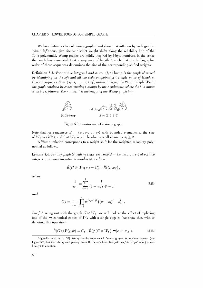
CHAPTER 5. LOWER BOUNDS FOR SIMPLE GRAPHS
We here define a class of Wump graphs1, and show that inflation by such graphs,Wump inflations, give rise to distinct weight shifts along the reliability line of theTutte polynomial. Wump graphs are mildly inspired by l-byte numbers, in the sensethat each has associated to it a sequence of length l, such that the lexicographicorder of these sequences determines the size of the corresponding shifted weights.
Definition 5.2. For positive integers i and s, an (i, s)-hump is the graph obtainedby identifying all the left and all the right endpoints of i simple paths of length s.Given a sequence S = 〈s1, s2, . . . , sl〉 of positive integers, the Wump graph WS isthe graph obtained by concatenating l humps by their endpoints, where the i-th humpis an (i, si)-hump. The number l is the length of the Wump graph WS .
(4, 2)-hump S = 〈3, 2, 3, 2〉
Figure 5.2: Construction of a Wump graph.
Note that for sequences S = 〈s1, s2, . . . , sl〉 with bounded elements si the sizeof WS is O(l2), and that WS is simple whenever all elements si ≥ 2.
A Wump-inflation corresponds to a weight-shift for the weighted reliability poly-nomial as follows.
Lemma 5.4. For any graph G with m edges, sequence S = 〈s1, s2, . . . , sl〉 of positiveintegers, and non-zero rational number w, we have
R(G⊗WS ;w) = CmS · R(G;wS) ,
where1
wS=
l∑i=1
1
(1 + w/si)i − 1(5.15)
and
CS =1
wS·
l∏i=1
w(si−1)i((w + si)
i − sii).
Proof. Starting out with the graph G⊗WS , we will look at the effect of replacingone of the m canonical copies of WS with a single edge e. We show that, with ϕdenoting this operation,
R(G⊗WS ;w) = CS · R(ϕ(G⊗WS);w[e 7→ wS ]) , (5.16)
1Originally, such as in [56], Wump graphs were called Bounce graphs for obvious reasons (seeFigure 5.2), but then the quoted passage from Dr. Seuss’s book One fish two fish red fish blue fish wasbrought to attention.
59
5.4. HARDNESS OF POINT EVALUATIONS
where wS satisfies (5.15), and w takes the old value w on all unaffected edges. Thelemma then follows by successively applying ϕ to each canonical copy of WS inG⊗WS .
The first step towards transforming a Wump graph (say, ) into a singleedge, is to contract each si-path of the i-th hump into a single edge, for i = 1, . . . , l.In other words, we perform the inverse of an si-stretch to the i-th hump. By (5.10)of Corollary 5.1, this ‘unstretching’ of the i-th hump contributes a factor (siw
si−1)i
to the polynomial, and each edge in the resulting (i, 1)-hump receives a weightof w/si. Repeating this process for each of the l humps in WS gives a simplifiedWump graph W 1
S generated by a sequence of 1s ( ). We let φ(G⊗WS)denote the graph obtained from G⊗WS by simplifying one canonical copy of WS
like this. By transitivity, we get the weight shift
R(G⊗WS ;w) =( l∏i=1
(siwsi−1)i
)· R(φ(G⊗WS);w′) ,
where w′ takes the value w/si on every edge of the ith hump of the simplifiedsubgraph W 1
S , and the old value w outside W 1S . Next, we replace each hump of W 1
S
by a single edge, to get a simple path ( ) of length l. This corresponds tothe inverse of an i-thickening for ith hump, for i = 1, . . . , l. By (5.11) of Corollary 5.1,this ‘unthickening’ does not produce any new factors for the polynomial, but theweight of the ith edge in the resulting path becomes
wi = (1 + w/si)i − 1 .
Finally, we compress the l-path into a single edge e, and the claim in (5.16) followsfrom Lemma 5.1 (i).
We now show that Wump inflations provide a rich enough class of weight shiftsw 7→ wS to provide points enough for interpolation. The ranges of w for whichwe prove this are general enough to allow for interpolation on the whole reliabilityline, and we make no attempt at extending the ranges.
Lemma 5.5. Let w be a rational number with w ∈ (−1, 0) or w ∈ (9,∞). For allintegers m ≥ 1, there exist integer sequences S0, . . . , Sm such that
(i) WSi is simple with O(log2m) edges for all i, and
(ii) wSi 6= wSj for all i 6= j, with wS as defined in (5.15).
Furthermore, such sequences Si can be computed in time polynomial in m.
Proof. Let r be a positive integer to be chosen later, only depending on w. Weconsider the set of sequences S = 〈s1, . . . , sl〉 of length l = r log(m + 1), suchthat si ∈ 2, 3 whenever i is a multiple of r, and si = 2 otherwise. Since r is aconstant and all si ≥ 2, this construction satisfies (i).
60
CHAPTER 5. LOWER BOUNDS FOR SIMPLE GRAPHS
Now consider any two distinct such sequences S = 〈si〉 and T = 〈ti〉. Toaddress (ii), we consider the difference
∆ =1
wS− 1
wT,
and show that ∆ 6= 0.Using Lemma 5.4 we get a sum expression for ∆,
∆ =l∑
i=1
1
(1 + w/si)i − 1−
l∑i=1
1
(1 + w/ti)i − 1
=l∑
i=1
g((1 + w/si)
i)−
l∑i=1
g((1 + w/ti)
i),
(5.17)
where g(x) = 1x−1 . This function is negative and strictly decreasing on (0, 1), and
positive and strictly decreasing on (1,∞). For convenience we let
a = min
(1 + w3
), (1 + w
2 )
and b = max
(1 + w3 ), (1 + w
2 ).
By the monotonicity of g we have g(ai) > g(bi) for all positive numbers i.Case 1: w > 9. Here we have a = (1 +w/3) and b = (1 +w/2). We set r = 1
and let k be the smallest index for which sk 6= tk . We can safely assume that sk = 3and tk = 2, otherwise just exchange the roles of S and T . Thus, in (5.17), terms of thesums for i < k cancel. The terms corresponding to i = k give g(ak) − g(bk) > 0.We apply the monotonicty of g to the terms for i > k, which allows us to lowerbound ∆ as follows,
∆ ≥
(g(ak) +
l∑i=k+1
g(bi)
)−
(g(bk) +
l∑i=k+1
g(ai)
)= f(a)− f(b) ,
where
f(x) = g(xk)−l∑
i=k+1
g(xi) =1
xk − 1−
l∑i=k+1
1
xi − 1. (5.18)
We now claim that f is strictly decreasing on (4,∞). This implies ∆ > 0, becausefor w > 9 we have 4 < a < b, and then ∆ ≥ f(a)− f(b) > 0. To prove this claim,consider
f ′(x) = − kxk−1
(xk − 1)2+
l∑i=k+1
ixi−1
(xi − 1)2. (5.19)
Let Ti(x) denote the ith term in this sum. For x > 4 we have
2Ti+1(x) < Ti(x) ,
61
5.4. HARDNESS OF POINT EVALUATIONS
because this inequality is equivalent to
2
(1 +
1
i
)x <
(x+
x− 1
xi − 1
)2
,
and in this expression we have LHS ≤ 4x < x2 ≤ RHS for all x > 4 and positiveintegers i. Thus, for x > 4 we can upper bounds the derivative in (5.19) as
f ′(x) <kxk−1
(xk − 1)2
(−1 +
l∑i=k+1
1
2i−k
)< 0 ,
which proves the claim.Case 2: w ∈ (−1, 0). Here we have a = (1 + w/2) and b = (1 + w/3).
We choose r to be a positive integer that satisfies br < 14 . Let rk be the smallest
index for which srk 6= trk . We assume w.l.o.g. that srk = 3 and trk = 2, otherwiseexchange the roles of S and T . In (5.17), terms of the sum for i < rk cancel, and sodo terms for those i’s that are not multiples of r. The terms corresponding to i = rkcontribute g(brk) − g(ark) < 0. We apply the monotonicty of g to the remainingterms for i > rk, which allows us to upper bound ∆ as follows,
∆ ≤
g(brk) +
l/r∑i=k+1
g(ari)
−g(ark) +
l/r∑i=k+1
g(bri)
,
where g(x) = 1x−1 . For x ∈ (0, 1), we can expand g(x) into the geometric series
g(x) = −∞∑j=0
xj .
Applying this representation to our estimate for ∆ and rearranging terms, we arriveat
∆ ≤∞∑j=0
(arj)k − (brj)k +
l/r∑i=k+1
((brj)i − (arj)i
)=
∞∑j=0
(F (arj)− F (brj)
),
where F is the function
F (y) = yk −l/r∑
i=k+1
yi .
We claim that F is strictly increasing on (0, 14). This implies ∆ < 0, because withthe given choice of r we have 0 < arj < brj < 1
4 for all positive integers j, and
62
CHAPTER 5. LOWER BOUNDS FOR SIMPLE GRAPHS
then F (arj) − F (brj) < 0 for j ≥ 1, and for j = 0 the term is 0. To prove thisclaim, consider
F ′(y) = kyk−1 −l/r∑
i=k+1
iyi−1 .
We obtain F ′(y) > 0 for y ∈ (0, 14) from the following calculation.
1
kyk−1·
l/r∑i=k+1
iyi−1 =
l/r∑i=k+1
i
kyi−k =
l/r−k∑i=1
(1 +
i
k
)yi
≤l/r−k∑i=1
(1 + i) yi ≤∞∑i=1
yi +∞∑i=1
iyi
=1
1− y− 1 +
y
(1− y)2≤ 4
3− 1 +
4
9< 1 .
5.4.2 Hardness of points on the reliability line
We are ready to prove Theorem 5.1. We consider the following equivalent claim.
Proposition 5.1. Let w 6= 0 be a rational number. Then, assuming #ETH, there is noexp(o(m/ log2m))-time algorithm computing the value of R(G;w) for simple inputgraphs G of m edges.
Proof. If w < −1, we can pick a positive integer k big enough such that
w′ := w/k > −1 .
This weight shift corresponds to the k-stretch of G by (5.10) of Corollary 5.1. On theother hand, if 0 < w < 9, we can pick a positive integer k such that
w′ := (w/2 + 1)k − 1 > 9 .
This weight shift corresponds to the 2-stretch of the k-thickening of G, by combiningthe weight shift identities of Corollary 5.1. In any case, the transformed graphG′ remains simple, the number of edges is increased by a constant factor of atmost 2k, and the value of R(G;w′) can be obtained in constant time from the valueof R(G′;w). Thus we can safely assume that w ∈ (−1, 0) or w > 9.
Now, by contradiction, suppose there was an exp(o(m/ log2m))-time algorithmfor evaluating R(G;w) for simple graphs G of m edges. Given such a graph G, wecan, according to Lemma 5.5, construct m+1 Wump graphs WS in polynomial time,such that each Wump inflation G⊗WS is simple with O(m log2m) edges, and suchthat the corresponding weight shifts w 7→ wS are all distinct. By Lemma 5.4, we couldthen use the assumed algorithm to compute R(G⊗WS ;w) ∼ R(G;wS) for eachWS , giving m+ 1 distinct evaluations of the mth-degree polynomial v 7→ R(G; v),and thus its coefficients by interpolation—all in time exp(o(m)). By Lemma 5.3there can be no such algorithm, unless #ETH fails.
63
5.4. HARDNESS OF POINT EVALUATIONS
64
Chapter 6
Lower Bounds for Planar Graphs
In this chapter we consider the restriction of Tutte(x, y) to planar input graphs.
Planar Tutte(x, y)
Input: A planar multigraph G with n vertices and m edges.Task: Compute T (G;x, y).
For this problem the complexity picture of the Tutte plane is slightly different. Oneof the most important differences is the hyperbola H2, i.e. the set of points (x, y)satisfying (x − 1)(y − 1) = 2, along which Planar Tutte(x, y) is polynomial-timesolvable, in addition to the trivial points for Tutte(x, y). This is a big thing intheoretical physics, because on this hyperbola the Tutte polynomial specializes tothe partition function of the so called Ising model (a.k.a. the 2-state Potts model).Vertigan [95] showed that that except for the hyperbolas H2, H1 and the points(−1,−1), (0,−1), (−1, 0), and (1, 1), every other point of the Tutte plane is#P-hard for Planar Tutte(x, y).
From the perspective of exponential-time complexity, the planar restriction givesan even more striking difference, because even at the #P-hard points, the problemPlanar Tutte(x, y) has an upper bound that is exponential only in O(
√n), due to an
algorithm by Sekine et al. [87]. A natural question is then whether this is optimalunder #ETH. To investigate this we will dig into the literature and look at existingstandard reductions with exponential-time glasses. We will see that the algorithm bySekine et al. is indeed optimal for the general problem, as a matching lower boundunder #ETH is found for points on the hyperbola H3. For remaining regions ofthe plane, lower bounds exponential in Ω(n1/k) are found under #ETH for variousk > 2. In particular, for points on the line y = 1 we get a lower bound exponentialin Ω(n1/8), which seems to be the first explicit superpolynomial lower bound also forthe general problem Tutte(x, 1). All bounds are shown to hold for graphs of O(n2)edges; see Figure 6.1 for an overview.
65

6.1. PLANAR TUTTE COMPUTATIONS
x−1 0 1
y
−1
0
1
no exp(o(√n)) , (§ 6.3.2)
no exp(o( 8√n)) , (§ 6.4.3)
no exp(o( 16√n)) , (§ 6.4.3)
no exp(o( 24√n)) , (§ 6.4.4)
no exp(o( 48√n)) , (§ 6.4.4)
nO(1) [59]
Figure 6.1: Exponential time complexity under #ETH of the Tutte plane for planar graphs interms of n, the number of vertices. All bounds hold in particular for graphs with m ∈ O(n2)edges.
6.1 Planar Tutte computations
It is generally considered one of the landmarks of statistical physics when Onsager [81]could give a closed form expression of the partition function of the Ising model (or2-state Potts model) for planar lattice graphs in 1944. A number of serious attemptswere made over the years to extend his result to other nontrivial graph classes, and toq-state Potts models for q > 2, but no progress was made. A vivid description of thefrustrations of these years can be found in the introduction of [58]. With our currentknowledge of computational tractability over the Tutte plane, and the relation (4.7)between the q-state Potts model and the Tutte polynomial along Hq , we now have anexplanation to the failure of these attempts. The #P-hardness map of the Tutte planeby Jaeger et al. [59] implies that Onsager’s result is unlikely to be extended to generalgraphs, and the corresponding #P-hardness map for planar graphs by Vertigan [95]implies that Onsager’s result is unlikely to be extended to q > 2 for planar graphs.
A subexponential upper bound From the previous chapters we know that, assum-ing #ETH, computation of T (G;x, y) for general fixed (x, y) requires time exponen-tial in the number of vertices or edges for multigraphs, and that for simple graphswe are within a polylogarithmic factor, in the exponent, of this bound. The situationfor the planar case is quite different, as there is a 2O(
√n)mO(1)-time algorithm by
Sekine et al. [87] from 1995. This situation is common to many other NP-hard prob-lems, such as Independent Set [77] and Hamiltonian Cycle [28] for which algorithmsexponential in O(
√n) are also known for planar graphs. These algorithms all use an
approach introduced by Lipton and Tarjan [76, 77], namely, a combination of dynamicprogramming and the planar separator theorem. This theorem states that in a pla-nar graph one can efficiently find a subset of O(
√n) vertices whose removal splits
the graph into components of size at most 2n/3. Without going into details, thealgorithm of Sekine et al. computes T (G;x, y) for planar G recursively, using thedeletion-contraction expansion of (4.13), and the planar separator theorem is involvedin finding a beneficial ordering of edges to be deleted-and-contracted, such that the
66
CHAPTER 6. LOWER BOUNDS FOR PLANAR GRAPHS
number of redundant computations can be more effectively reduced compared to thecase of a general recursion tree.
6.1.1 Main theorems
The question under consideration here is whether the 2O(√n)mO(1)-time algorithm
for Planar Tutte(x, y) by Sekine et al. has an asymptotically optimal dependency onthe number n of vertices, assuming #ETH. As remarked in Section 4.3.2, the numberm of edges for a general input graph could in fact be exponential in n, so we needto make sure that any lower bound in terms of n holds for graphs that are not toodense.
In [29], an almost complete map of the exponential-time complexity across theTutte plane for both multigraphs and simple graphs was presented. This was achievedby finding exact, exponential-time-preserving, versions of reductions in Goldberg andJerrum’s paper [48], concerning NP-hardness of approximation. Motivated by thissuccess, a similar translation of the same authors’ reductions for the planar case in[49] was sought. This worked out only for points on the hyperbola H3, which issomewhat surprising as the upper branch of this hyperbola was not covered by theinapproximability result of [49].
Theorem 6.1. Let (x, y) ∈ Q2 with (x−1)(y−1) = 3 and y 6= −1. Then, assuming#ETH, there is no exp(o(
√n))-time algorithm for Planar Tutte(x, y). The bound holds
especially for input graphs of O(n2) edges.
Consequently, the algorithm by Sekine et al. is indeed optimal for the generalproblem Planar Tutte(x, y), assuming #ETH. Proofs are given in Section 6.3.
Unfortunately, the idea of the reduction in [49] that covers the main regionsof the plane seems to not lend itself easily to our purpose; see discussion in sec-tion 6.5.2. Instead, the #P-hardness reductions of Vertigan [95] were studied, whichled to conditional lower bounds of the type exp(Ω(n1/k)) for various k > 2. Theconclusions are contained in the following theorem. These bounds leave the questionof exponential-time complexity of Planar Tutte(x, y) very much open for most of theTutte plane, but are included here for a complete picture of the current situation.
Theorem 6.2. Let (x, y) ∈ Q2 with (x − 1)(y − 1) /∈ 1, 2, 3. Then, assuming#ETH, there is no algorithm for Planar Tutte(x, y) with running time
(i) exp(o( 8√n)) if y = 1 and x 6= 1,
(ii) exp(o( 16√n)) if x = 1 and y 6= 1,
(iii) exp(o( 24√n)) for any remaining point with x 6= 1 and y /∈ 0,−1,
(iv) exp(o( 48√n)) for any remaining point with x 6= 1 and y ∈ 0,−1, even for
simple planar graphs.
The bounds hold especially for input graphs of O(n2) edges.
67

6.2. PRELIMINARIES
Proofs are in Section 6.4. The result for the line y = 1 is of particular interest,as this seems to be the first concrete superpolynomial lower bound also for the moregeneral problem Tutte(x, 1). In fact, the only proof of #P-hardness of Tutte(x, 1) seemsto rely on the hardness proof for the planar case.
6.1.2 Related work
The stuff of this chapter builds heavily on two papers.The first, by Goldberg and Jerrum [49], shows hardness of approximation of
Planar Tutte(x, y) for large regions of the Tutte plane, in the sense of excluding afully polynomial randomized approximation scheme (FPRAS) under the assumptionthat RP 6=NP. This was a follow-up on their previous work [48] on general graphs.
The second paper, by Vertigan [95]1, contains the mentioned result of #P-hardnessfor every point of the Tutte plane except those on H1, H2 and the points (−1,−1),(0,−1), (−1, 0), and (1, 1). In fact, Vertigan’s results are explicitly stated for anyalgebraic point (x, y), an extension that we will also use at one point.
6.2 Preliminaries
Reductions in this chapter will repeatedly involve the problem of finding coefficientsof various graph polynomial s 7→ p(G; s) for planar graphs G. We let [sd]p(G; s)denote the coefficient of sd in p(G; s). Below we give some basic properties ofplanar graphs that we will use.
Euler’s equation. Euler’s equation says that if n,m, f denote the number of ver-tices, edges and faces, respectively, of a planar graph G, then
n−m+ f = 2 . (6.1)
In the case that the planar graph G is also simple, then each face is bounded by atleast three edges, and we get
m ≤ 3n+ 6 . (6.2)
The Tutte polynomial for dual graphs. A given planar graph G may have differentnon-isomorphic duals G∗, resulting from different planar drawings of G, but the Tuttepolynomial is blind to this difference due to the following pleasant property,
T (G;x, y) = T (G∗; y, x) . (6.3)
This identity is classically used for mirroring hardness results over the line y = xin the Tutte plane. However, for exponential-time complexity we must use this withcaution, because, unless G is of bounded degree, the number of faces f in G, andthus the number n∗ = f of vertices in G∗, may be much larger than n.
1This work appeared already in Vertigan’s PhD thesis from 1991 [94].
68

CHAPTER 6. LOWER BOUNDS FOR PLANAR GRAPHS
6.3 The 3-state Potts hyperbola
To prove Theorem 6.1 we start out from a coloring problem. The same approach isused in [49, Section 4].
6.3.1 Planar 3-coloring
We give a lower bound for the planar version of the following classical problem.
3-Coloring
Input: A simple graph G with n vertices and m edges.Task: Decide whether there is a proper 3-coloring of G.
For general simple graphs, an edge-exponential lower bound under ETH was givenalready in [57]. In [30], this result was extended to the counting version #3-Coloringunder #ETH.
Theorem 6.3 (Dell et al. [30]). Assuming #ETH, there is no exp(o(m))-time algorithmfor #3-Coloring.
We consider the restriction of this problem to planar graphs, #Planar 3-Coloring,and show the following corresponding lower bound.
Theorem 6.4. Assuming #ETH, there is no exp(o(√n))-time algorithm for #Planar
3-Coloring.
Note that for connected, simple, planar graphs we have n ≤ m ≤ 3n − 6 byEuler’s equation, so this bound is equivalent to the same bounds in terms of m.Thus, given Theorem 6.3, it is enough to find a reduction from #Planar 3-Coloring toits planar counterpart, such that the number of edges does not increase too much.This is provided by the following lemma.
Lemma 6.1. There is a mapping reduction from #3-Coloring to #Planar 3-Coloring,mapping graphs of m edges to graphs of O(m2) edges.
Proof. We show that the claim is satisfied by a standard reduction from 3-Coloring toPlanar 3-Coloring in [44], if we replace the crossover gadget used in [44] by the graphW shown in Figure 6.2, which was introduced in [3] to preserve information aboutthe number of colorings.
Figure 6.2: W , with con-nection vertices in black.
Given a simple input graph G to #3-Coloring, consider a drawing of G in theplane such that at most two edges cross at any given point. A simple planar graphG′ is constructed from this drawing by successively picking an edge that is crossedby other edges, along this edge replacing each crossing by a copy of the gadget W ,without introducing new edge intersections; see Figure 6.3. It is shown in [3] that Ghas k proper 3-colorings if, and only if, G′ has k · 2c(G) proper 3-colorings, wherec(G) is the number of edge-intersections in the drawing of G. We note that thenumber of edges of G′ satisfies m′ ≤ m + 31c(G). Since c(G) < m2 for simplegraphs G, this means m′ ∈ O(m2). The claim follows.
69
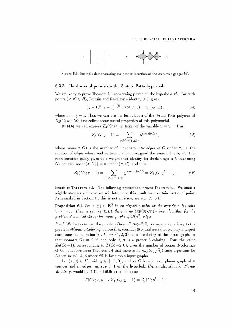
6.3. THE 3-STATE POTTS HYPERBOLA
W W W
Figure 6.3: Example demonstrating the proper insertion of the crossover gadget W .
6.3.2 Hardness of points on the 3-state Potts hyperbola
We are ready to prove Theorem 6.1, concerning points on the hyperbola H3. For suchpoints (x, y) ∈ H3, Fortuin and Kasteleyn’s identity (4.9) gives
(y − 1)n(x− 1)κ(E)T (G;x, y) = Z3(G;w) , (6.4)
where w = y − 1. Thus we can use the formulation of the 3-state Potts polynomialZ3(G;w). We first collect some useful properties of this polynomial.
By (4.6), we can express Z3(G;w) in terms of the variable y = w + 1 as
Z3(G; y − 1) =∑
σ:V→1,2,3
ymono(σ,G) , (6.5)
where mono(σ,G) is the number of monochromatic edges of G under σ, i.e. thenumber of edges whose end vertices are both assigned the same value by σ. Thisrepresentation easily gives us a weight-shift identity for thickenings: a k-thickeningGk satisfies mono(σ,Gk) = k ·mono(σ,G), and thus
Z3(Gk; y − 1) =∑
σ:V→1,2,3
yk·mono(σ,G) = Z3(G; yk − 1) . (6.6)
Proof of Theorem 6.1. The following proposition proves Theorem 6.1. We state aslightly stronger claim, as we will later need this result for a certain irrational point.As remarked in Section 4.3 this is not an issue; see e.g. [59, p.41].
Proposition 6.1. Let (x, y) ∈ R2 be an algebraic point on the hyperbola H3 withy 6= −1. Then, assuming #ETH, there is no exp(o(
√n))-time algorithm for the
problem Planar Tutte(x, y) for input graphs of O(n2) edges.
Proof. We first note that the problem Planar Tutte(−2, 0) corresponds precisely to theproblem #Planar 3-Coloring. To see this, consider (6.5) and note that we may interpreteach state configuration σ : V → 1, 2, 3 as a 3-coloring of the input graph, sothat mono(σ,G) = 0 if, and only if, σ is a proper 3-coloring. Thus the valueZ3(G;−1), corresponding to T (G;−2, 0), gives the number of proper 3-coloringsof G. It follows from Theorem 6.4 that there is no exp(o(
√n))-time algorithm for
Planar Tutte(−2, 0) under #ETH for simple input graphs.Let (x, y) ∈ H3 with y /∈ −1, 0, and let G be a simple, planar graph of n
vertices and m edges. As x, y 6= 1 on the hyperbola H3, an algorithm for PlanarTutte(x, y) would by (6.4) and (6.6) let us compute
T (Gk;x, y) ∼ Z3(Gk; y − 1) = Z3(G; yk − 1)
70
CHAPTER 6. LOWER BOUNDS FOR PLANAR GRAPHS
for k = 1, . . . ,m+ 1. Since y /∈ 0, 1,−1 this gives m+ 1 distinct evaluations ofthe mth degree polynomial w 7→ Z3(G;w), and thus we could get the coefficientsby interpolation. This in turn would let us evaluate Z3(G; 0), which by the abovediscussion cannot be done in time exp(o(
√n)) under #ETH. As G is simple and
planar, Euler’s equation gives m ∈ O(n), so the thickened graph Gk will have nvertices and km ∈ O(n2) edges for any k ≤ m+ 1, and the claim follows.
6.4 The rest of the plane
For the remaining points of the plane we turn to the work done by Vertigan [95]concerning #P-hardness for Planar Tutte(x, y). These results rely on a hardness resultby Provan [83] of computing two-terminal network reliability—a concept related tothe all-terminal reliability studied in Chapter 5—which in turn relies on the hardnessof counting Hamiltonian cycles in cubic graphs.
6.4.1 Hardness of Hamiltonian cycles in cubic planar graphs
We consider the following problem.
#Planar Cubic Hamiltonian Cycle
Input: A cubic, planar graph G with n vertices and m edges.Task: Find the number of Hamiltonian cycles in G.
The decision version of this problem was shown NP-hard in [46] by reduction from3-Sat. Provan [83] noted that the same reduction shows #P-hardness of #Planar CubicHamiltonian Cycle by reduction from #3-Sat. In fact, it is made explicit in [46, p.711]that the construction maps a 3-CNF formula ϕ of n variables to a cubic planar graphG of O(n2) vertices. Thus we have the following conditional lower bound.
Theorem 6.5. Assuming #ETH, there is no exp(o(√n))-time algorithm for the prob-
lem #Planar Cubic Hamiltonian Cycle.
6.4.2 Hardness of two-terminal reliability
Like the concept of all-terminal network reliability defined in the previous chapter,the two-terminal version also considers a connected graph G = (V,E) with edgefailure probability p, but instead of the probability R(G; p) that the full graph Gstays connected, we are given two vertices s, t ∈ V and consider the probabilityRs,t(G; p) that s and t remain connected by a path. We can express this probabilityas
Rs,t(G; p) =∑A⊆E
s,t connected
p|A|(1− p)|E|−|A| . (6.7)
Note that the sum in (6.7) is taken over all edge subsets containing an (s, t)-path; welet Es,t(G) denote the collection of all such subsets. We will ultimately be interested
71

6.4. THE REST OF THE PLANE
in the problem of computing the size of this set. From (6.7) we see that
|Es,t(G)| = 2|E|Rs,t(G; 1/2) . (6.8)
For a given probability p, define the problem
∆3-Planar Path Reliability(p)
Input: A planar graph G = (V,E) of maximum degree threewith n vertices and m edges and s, t ∈ V .
Task: Compute Rs,t(G; p).
In [83], #P-hardness of this problem is shown by reduction from #Planar CubicHamiltonian Cycle. We obtain the following lower bound.
Proposition 6.2. Let p ∈ (0, 1) be a fixed rational number. Assuming #ETH, thereis no exp(o( 4
√n))-time algorithm for the problem ∆3-Planar Path Reliability(p). In
particular, the bound applies to computation of |Es,t(G)|.
To prove this, we study the vertex expansion of the reduction in [83].
Provan’s reductions. There are two steps to the reduction in [83]. The first stepconcerns a certain intermediate quantity called Rs,t(G,S, l, k), defined for a graphG = (V,E) with terminals s, t ∈ V , an edge subset S ⊆ E, and numbers l, k ∈ N.In [83, p.697], this quantity is related to Rs,t(G; p) by the equation
Rs,t(Gq,r; p) =
∑i,j
(−pq+1)i(−pr+1)jRs,t(G,S, i, j) , (6.9)
where Gq,r is the graph obtained from G by (q+ 1)-stretching every edge in S and(r + 1)-stretching every edge in E \ S.
Define the problem
∆3-Planar ProvanInput: A planar graph G = (V,E) of maximum degree three, with
n vertices, s, t ∈ V , a subset S ⊆ E , and numbers l, k ∈ N.Task: Compute Rs,t(G,S, l, k).
The first step of the reduction is the following result.
Lemma 6.2 (Theorem 1 in [83]). There is a mapping reduction from #Planar CubicHamiltonian Cycle to the problem ∆3-Planar Provan that maps graphs of n vertices tographs of 3n+ 2 vertices.
This fact, together with the following lemma and the exp(Ω(√n))-time lower
bound for #Planar Cubic Hamiltonian Cycle of Theorem 6.5, proves Proposition 6.2.
Lemma 6.3. For any probability p ∈ (0, 1) there is a polynomial-time reduction fromthe problem ∆3-Planar Provan to ∆3-Planar Path Reliability(p) that maps graphs of nvertices to sets of graphs of O(n2) vertices each.
72
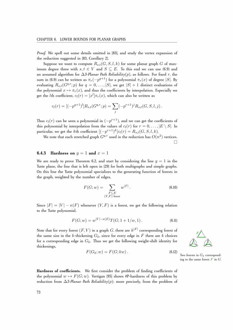
CHAPTER 6. LOWER BOUNDS FOR PLANAR GRAPHS
Proof. We spell out some details omitted in [83], and study the vertex expansion ofthe reduction suggested in [83, Corollary 2].
Suppose we want to compute Rs,t(G,S, l, k) for some planar graph G of max-imum degree three with s, t ∈ V and S ⊆ E. To this end we can use (6.9) andan assumed algorithm for ∆3-Planar Path Reliability(p), as follows. For fixed r, thesum in (6.9) can be written as πr(−pq+1) for a polynomial πr(x) of degree |S|. Byevaluating Rs,t(Gq,r; p) for q = 0, . . . , |S|, we get |S| + 1 distinct evaluations ofthe polynomial x 7→ πr(x), and thus the coefficients by interpolation. Especially weget the lth coefficient, cl(r) = [xl]πr(x), which can also be written as
cl(r) = [(−pq+1)l]Rs,t(Gq,r; p) =
∑j
(−pr+1)jRs,t(G,S, l, j) .
Thus cl(r) can be seen a polynomial in (−pr+1), and we can get the coefficients ofthis polynomial by interpolation from the values of cl(r) for r = 0, . . . , |E \ S|. Inparticular, we get the kth coefficient [(−pr+1)k]cl(r) = Rs,t(G,S, l, k).
We note that each stretched graph Gq,r used in the reduction has O(n2) vertices.
6.4.3 Hardness on y = 1 and x = 1
We are ready to prove Theorem 6.2, and start by considering the line y = 1 in theTutte plane, the line that is left open in [29] for both multigraphs and simple graphs.On this line the Tutte polynomial specializes to the generating function of forests inthe graph, weighted by the number of edges,
F (G;w) =∑F⊆E
(V,F ) forest
w|F | . (6.10)
Since |F | = |V | − κ(F ) whenever (V, F ) is a forest, we get the following relationto the Tutte polynomial,
F (G;w) = w|V |−κ(E)T (G; 1 + 1/w, 1) . (6.11)
Note that for every forest (F, V ) in a graph G, there are k|F | corresponding forest ofthe same size in the k-thickening Gk , since for every edge in F there are k choicesfor a corresponding edge in Gk . Thus we get the following weight-shift identity forthickenings,
F (Gk;w) = F (G; kw) . (6.12)
F
Two forests in G2 correspond-ing to the same forest F in G.
Hardness of coefficients. We first consider the problem of finding coefficients ofthe polynomial w 7→ F (G;w). Vertigan [95] shows #P-hardness of this problem byreduction from ∆3-Planar Path Reliability(p); more precisely, from the problem of
73
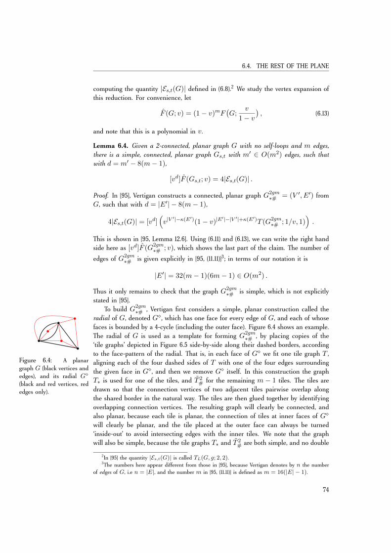
6.4. THE REST OF THE PLANE
computing the quantity |Es,t(G)| defined in (6.8).2 We study the vertex expansion ofthis reduction. For convenience, let
F (G; v) = (1− v)mF(G;
v
1− v), (6.13)
and note that this is a polynomial in v.
Lemma 6.4. Given a 2-connected, planar graph G with no self-loops and m edges,there is a simple, connected, planar graph Gs,t with m′ ∈ O(m2) edges, such thatwith d = m′ − 8(m− 1),
[vd]F (Gs,t; v) = 4|Es,t(G)| .
Proof. In [95], Vertigan constructs a connected, planar graph G2gm∗# = (V ′, E′) from
G, such that with d = |E′| − 8(m− 1),
4|Es,t(G)| = [vd](v|V
′|−κ(E′)(1− v)|E′|−|V ′|+κ(E′)T (G2gm
∗# ; 1/v, 1)).
This is shown in [95, Lemma 12.6]. Using (6.11) and (6.13), we can write the right handside here as [vd]F (G2gm
∗# ; v), which shows the last part of the claim. The number of
edges of G2gm∗# is given explicitly in [95, (11.11)]3; in terms of our notation it is
|E′| = 32(m− 1)(6m− 1) ∈ O(m2) .
Thus it only remains to check that the graph G2gm∗# is simple, which is not explicitly
stated in [95].To build G2gm
∗# , Vertigan first considers a simple, planar construction called theradial of G, denoted G, which has one face for every edge of G, and each of whosefaces is bounded by a 4-cycle (including the outer face). Figure 6.4 shows an example.
Figure 6.4: A planargraph G (black vertices andedges), and its radial G
(black and red vertices, rededges only).
The radial of G is used as a template for forming G2gm∗# , by placing copies of the
‘tile graphs’ depicted in Figure 6.5 side-by-side along their dashed borders, accordingto the face-pattern of the radial. That is, in each face of G we fit one tile graph T ,aligning each of the four dashed sides of T with one of the four edges surroundingthe given face in G, and then we remove G itself. In this construction the graphT∗ is used for one of the tiles, and T 2
# for the remaining m − 1 tiles. The tiles aredrawn so that the connection vertices of two adjacent tiles pairwise overlap alongthe shared border in the natural way. The tiles are then glued together by identifyingoverlapping connection vertices. The resulting graph will clearly be connected, andalso planar, because each tile is planar, the connection of tiles at inner faces of G
will clearly be planar, and the tile placed at the outer face can always be turned‘inside-out’ to avoid intersecting edges with the inner tiles. We note that the graphwill also be simple, because the tile graphs T∗ and T 2
# are both simple, and no double
2In [95] the quantity |Es,t(G)| is called TL(G, g; 2, 2).3The numbers here appear different from those in [95], because Vertigan denotes by n the number
of edges of G, i.e n = |E|, and the number m in [95, (11.11)] is defined as m = 16(|E| − 1).
74
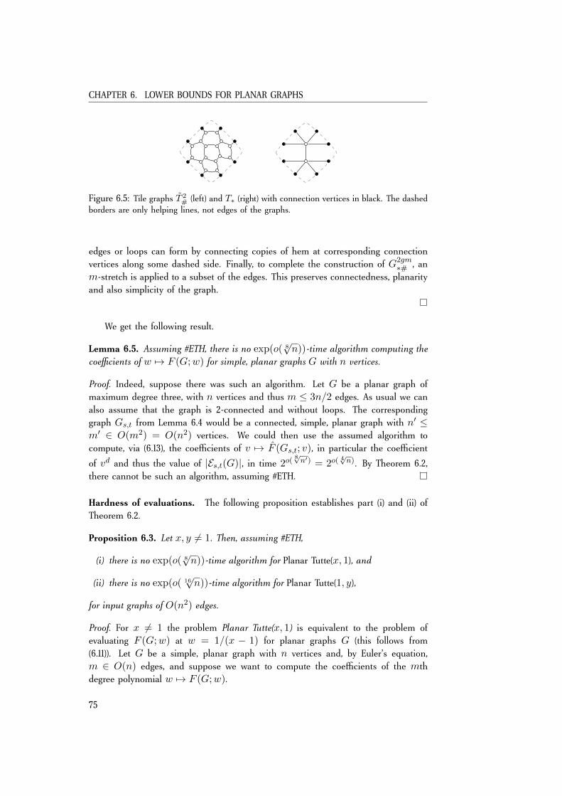
CHAPTER 6. LOWER BOUNDS FOR PLANAR GRAPHS
Figure 6.5: Tile graphs T 2# (left) and T∗ (right) with connection vertices in black. The dashed
borders are only helping lines, not edges of the graphs.
edges or loops can form by connecting copies of hem at corresponding connectionvertices along some dashed side. Finally, to complete the construction of G2gm
∗# , anm-stretch is applied to a subset of the edges. This preserves connectedness, planarityand also simplicity of the graph.
We get the following result.
Lemma 6.5. Assuming #ETH, there is no exp(o( 8√n))-time algorithm computing the
coefficients of w 7→ F (G;w) for simple, planar graphs G with n vertices.
Proof. Indeed, suppose there was such an algorithm. Let G be a planar graph ofmaximum degree three, with n vertices and thus m ≤ 3n/2 edges. As usual we canalso assume that the graph is 2-connected and without loops. The correspondinggraph Gs,t from Lemma 6.4 would be a connected, simple, planar graph with n′ ≤m′ ∈ O(m2) = O(n2) vertices. We could then use the assumed algorithm tocompute, via (6.13), the coefficients of v 7→ F (Gs,t; v), in particular the coefficient
of vd and thus the value of |Es,t(G)|, in time 2o(8√n′) = 2o(
4√n). By Theorem 6.2,there cannot be such an algorithm, assuming #ETH.
Hardness of evaluations. The following proposition establishes part (i) and (ii) ofTheorem 6.2.
Proposition 6.3. Let x, y 6= 1. Then, assuming #ETH,
(i) there is no exp(o( 8√n))-time algorithm for Planar Tutte(x, 1), and
(ii) there is no exp(o( 16√n))-time algorithm for Planar Tutte(1, y),
for input graphs of O(n2) edges.
Proof. For x 6= 1 the problem Planar Tutte(x, 1) is equivalent to the problem ofevaluating F (G;w) at w = 1/(x − 1) for planar graphs G (this follows from(6.11)). Let G be a simple, planar graph with n vertices and, by Euler’s equation,m ∈ O(n) edges, and suppose we want to compute the coefficients of the mthdegree polynomial w 7→ F (G;w).
75
6.4. THE REST OF THE PLANE
(i) By the thickening identity (6.12), an algorithm for Planar Tutte(x, 1) could beused to compute F (Gk;w) = F (G; kw) for k = 1, . . . ,m + 1, giving m + 1distinct evaluations of w 7→ F (G;w) and thus the coefficients by interpolation. AsGk has n vertices and O(m2) = O(n2) edges for k ≤ m + 1, the given boundfollows from Lemma 6.5.
(ii) By (6.3) we have T (G∗k; y, 1) = T (Gk; 1, y) for any planar dual G∗k ofGk . Thus the above interpolation procedure for obtaining the coefficients of w 7→F (G;w) could be performed also with an algorithm for Planar Tutte(1, y). Wenote that G∗k will be a connected graph with the same number m′ ∈ O(n2) ofedges as Gk , and, by Euler’s theorem, with n∗ ∈ O(m′) ⊂ O(n2) vertices. Theclaimed bound for Planar Tutte(1, y) then follows from the above bound for PlanarTutte(x, 1).
6.4.4 Hardness for remaining points
Finally we consider points on hyperbolas Hq for remaining rationals q /∈ 0, 1, 2, 3.For technical simplification we will use the formulation of the multivariate Tuttepolynomial defined in (4.10). Recall that T (G;x, y) is computationally equivalent toZ(G; q, w), with q = (x− 1)(y − 1) and w = y − 1, whenever q 6= 0.
Hardness of coefficients. We first consider the problem of finding coefficientsof the polynomial w 7→ Z(G; q, w) for planar graphs. Vertigan [95] shows #P-hardness also of this problem by reduction from two-terminal reliability. However,this reduction gives a much worse vertex expansion than the corresponding reductionfor the forest-counting polynomial. To get a somewhat better superpolynomial lowerbound, we will instead use Proposition 6.1 and reduce from a point on the hyperbolaH3. We first use an intermediate reduction from [95].
Let
Z(G; q, v) = (1− v)|E|q−|V |Z(G; q, qv/(1− v)) , (6.14)
and note that this is a polynomial in v.
Lemma 6.6. Given a connected, planar graph G with n vertices and m edges, anda natural number k, there is a simple, connected, planar graph G〈k〉 with m′ ∈O(k4m2) edges, such that with d = m′ − 2k2m and xk = 1 + (q − 1)k ,
[vd]Z(G〈k〉; q, v) = (q − 1)k·κ(E)T (G;xk, xk) .
Proof. In [95], a graph called Gk# is constructed by glueing together copies of a
certain tile graph T k# in the same fashion as described in the proof of Lemma 6.4.
The graph T k# is a generalization of the graph T 2# in Figure 6.5 to 4k connection
vertices, with the same grid-like structure. Thus Gk# will also be connected, simpleand planar.
76

CHAPTER 6. LOWER BOUNDS FOR PLANAR GRAPHS
Let (V ′, E′) = Gk#. From [95, (11.2)]4 it follows that
|E′| = 8k3(k + 1)m2 + 4k2m ∈ O(k4m2) ,
and it is shown in [95, Lemma 12.3] that with d = |E′| − 2k2m,
(q − 1)k·κ(E)T (G;xk, xk) = [vd]CvT
(Gk#;
1
v, 1 +
qv
1− v
),
where Cv = vn′−κ(E′)(1 − v)m
′−n′+κ(E′). The expression on the right hand sidecan also be written as [vd]Z(Gk#; q, v).
We get the following result.
Lemma 6.7. Let q /∈ 0, 1, 2. Then, assuming #ETH, there is no exp(o( 24√n))-time
algorithm computing the coefficients of w 7→ Z(G; q, w) for simple, planar graphs Gof n vertices.
Proof. Let α = 1+√
3, and note that (α, α) ∈ H3 and that this is an algebraic point.It follows from Proposition 6.1 that there can be no exp(o(
√n))-time algorithm for
Planar Tutte(α, α) under #ETH, even when restricted to graphs of m ∈ O(n2) edges.As (α, α) is a point on the line y = x in the Tutte plane, the same lower boundmust then apply to the problem of computing the coefficients of x 7→ T (G;x, x)for planar graphs G with O(n2) edges. This is the starting point.
Now suppose there was an exp(o( 24√n))-time algorithm computing the coef-
ficients of w 7→ Z(G; q, w) for planar graph with O(n2) edges. Let G be sucha graph, let k ≤ m + 1, and consider the corresponding connected, simple, pla-nar graph G〈k〉 as defined in Lemma 6.6. Since G has m ∈ O(n2) edges, thegraph G〈k〉 has n′ ≤ m′ ∈ O(m2k4) ⊆ O(n12) vertices, according to Lemma 6.6.We could then use the assumed algorithm to compute, via (6.14), the coefficients ofv 7→ Z(G〈k〉; q, v). In particular, we would get the coefficient of vd and thus thevalue of T (G;xk, xk), with xk = 1 + (q − 1)k and d as defined in Lemma 6.6,since q 6= 1. Repeating this procedure for k = 1, . . . ,m + 1 would provide m + 1evaluations of the mth degree polynomial x 7→ T (G;x, x), and these evaluationswould all be distinct since q /∈ 0, 1, 2. Hence we could get the full polynomialx 7→ T (G;x, x) by interpolation. The claim then follows from the above discus-sion.
Hardness of evaluations. The following proposition establishes part (iii) and (iv) ofTheorem 6.2.
Proposition 6.4. Let (x, y) be a nontrivial point in the Tutte plane with q =(x − 1)(y − 1) /∈ 0, 1, 2. Then, assuming #ETH, there is no algorithm for Pla-nar Tutte(x, y) with running time
4Again, in [95] Vertigan denotes by n the number of edges of G, i.e n = |E|, and the number m in[95, (11.2)] is defined as m = 4k2n.
77
6.5. DISCUSSION
(i) exp(o( 24√n)) if x 6= 1 and y /∈ 0,−1 for input graphs of O(n2) vertices,
(ii) exp(o( 48√n)) if x 6= 1 and y ∈ 0,−1 for simple input graphs.
Proof. Let G be a connected, simple, planar graph with n vertices and m ∈ O(n)edges (by Euler’s equation), and suppose we want to compute the coefficients of themth degree polynomial w 7→ Z(G; q, w). Recall that for q 6= 0 the problem PlanarTutte(x, y) is computationally equivalent to evaluation of Z(G; q, w) at w = y − 1for planar graphs G.
(i) For y /∈ 0,−1, corresponding to w /∈ −1,−2, we use thickening andinterpolation. By (4.19) a k-thickening for the multivariate Tutte polynomial corre-sponds to the weight shift w 7→ (1 + w)k − 1, so we get distinct weight shiftsfor distinct values of k for the given restriction on w. Thus we could apply analgorithm for Planar Tutte(x, y) to input graphs Gk for k = 1, . . . ,m + 1, to getm + 1 distinct evaluations Z(Gk; q, w) = Z(G; q, wk), and then the coefficientsof w 7→ Z(G; q, w) by interpolation. As Gk has n vertices and O(m2) ⊂ O(n2)edges for all k ≤ m+ 1, the result follows from Lemma 6.7.
(ii) For y ∈ 0,−1, corresponding to w ∈ −1,−2 we use the same argumentwith stretches instead of thickenings. Note that since G is simple and planar, thegraph Gk is also simple and planar with O(m2) = O(n2) vertices for any k ≤ m+1.By (4.18), a k-stretch for the multivariate Tutte polynomial corresponds to a weightshift w 7→ w′, where (1 + q/w′) = (1 + q/w)k . We must ensure that distinctvalues of k gives gives distinct weight shifts. For w = −1 this is true providedq /∈ 1, 2, which holds by assumption. For w = −2 this is true provided q /∈ 2, 4,which also holds by assumption since (w, q) = (−2, 4) corresponds to the point(x, y) = (−1,−1), which is a trivial point in the Tutte plane and thus excluded byassumption. The result then follows from Lemma 6.7.
6.5 Discussion
From Theorem 6.1 we have an asymptotically tight lower bound for the problem PlanarTutte(x, y) for points on the hyperbola H3. Compared to this result, the bounds forother regions of the plane provided by Theorem 6.2 certainly leave substantial gapsto the O(
√n)-exponential upper bound. There is no apparent reason why points on
the hyperbola H3 should present much harder problems than points on any othercurve in the Tutte plane, so it seems likely that the lower bounds of Theorem 6.2can be significantly improved. In this section we look at some approaches to thisproblem, as well as obstacles that were encountered.
6.5.1 The chromatic line
On the chromatic line y = 0, the Tutte polynomial specializes to the chromaticpolynomial χ(G;x) defined in (4.3). For points on this line we only have a lowerbound exponential in Ω( 48
√n) under #ETH from Theorem 6.2(iii), except for the
78
CHAPTER 6. LOWER BOUNDS FOR PLANAR GRAPHS
point (−2, 0) where a tight lower bound exponential in Ω(√n) follows from Theo-
rem 6.1. For both multigraphs and simple graphs this one point (−2, 0) determinesthe exponential-time complexity of any other point on the chromatic line, by a well-known reduction due to Linial [75], based on the following identity:
Theorem 6.6 (Linial [75]). Let i ∈ 1, 2, . . . and let r be any real number. Then
χ(G+Ki; r) = r(r − 1) . . . (r − i+ 1) · χ(G; r − i) , (6.15)
where G + Ki is the graph consisting of G and a clique Ki on i vertices, each ofwhich is adjacent to every vertex of G.
For planar graphs we cannot use this reduction, as the graphs G + Ki are verynonplanar in general. It would be interesting to find a planarity-preserving reductionfor the chromatic line.
The status of line is particularly intriguing as there can only be a finite numberof points on it where the tight lower bound does not hold, considering the remark inSection 4.3.2.
6.5.2 Coefficients via #3-Terminal Min-Cut
The lower bounds of Theorem 6.2 (iii) and (iv) are particularly far from the upperbound. This is due to the exp(Ω( 24
√n))-time lower-bound of Lemma 6.7 for com-
puting coefficients of w 7→ Z(G; q, w) for simple planar graphs. We can comparethis to Lemma 5.3 of the previous chapter, which gives a lower bound of exp(Ω(m))under #ETH, for the same problem for general simple graphs. That bound, as wellas the approximation-hardness result of [48], rests ultimately on the hardness of thefollowing problem
Simple #3-Terminal Min-Cut
Input: A simple graph G = (V,E) with n vertices, m edgesand terminals t1, t2, t3 ∈ V .
Task: Find the number of cuts of minimum size such thatt1, t2 and t3 are in distinct components.
Dahlhaus et al. [26] showed that the decision version of this problem is NP-complete,and a lower bound of exp(Ω(m)) for the counting version under #ETH follows in[29, Theorem C.1]. However, Dahlhaus et al. also showed that the decision problemPlanar 3-Terminal Min-Cut is in P, which leaves the status of the counting versionopen for planar graphs. It may very well be in FP.
Moreover, even if Simple #3-Terminal Min-Cut would be hard also for planargraphs, the reduction to the coefficient problem used for Lemma 5.3 is not planaritypreserving. The first step of this reduction is the proof of [30, Lemma 1], where threenew edges are added to the input graph G to Simple #3-Terminal Min-Cut. Then, forLemma 5.3, these newly added edges would be removed again using deletions and
79
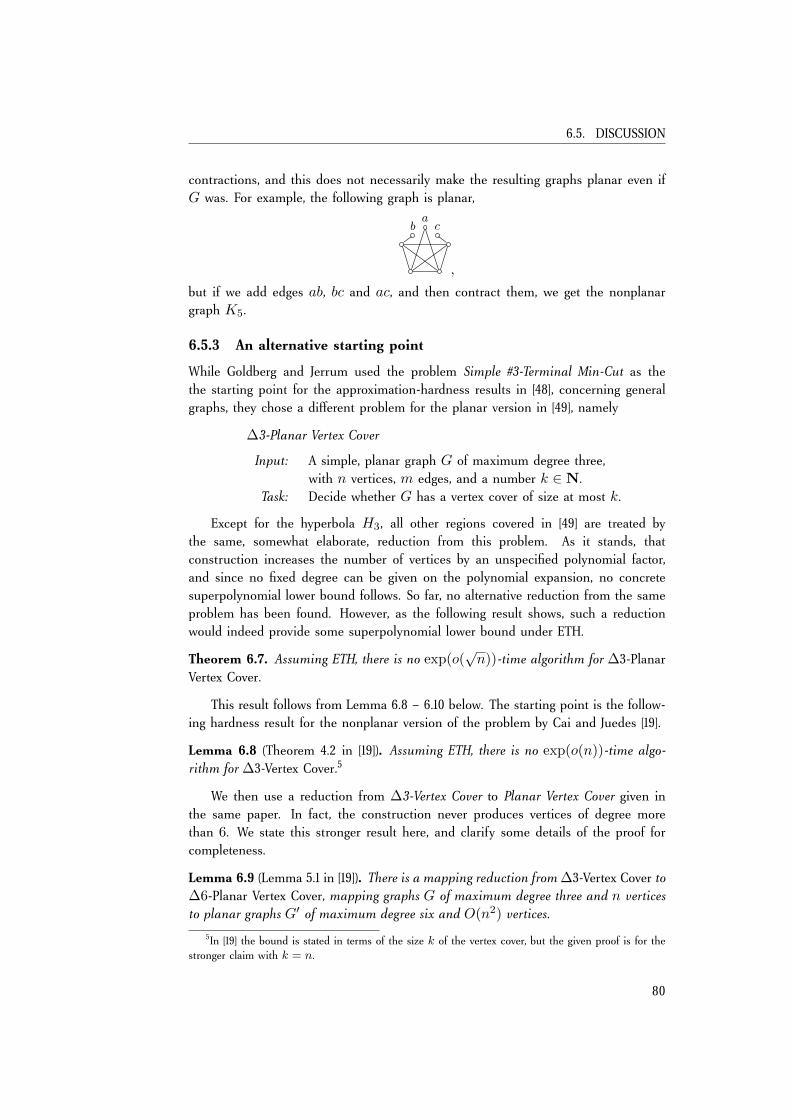
6.5. DISCUSSION
contractions, and this does not necessarily make the resulting graphs planar even ifG was. For example, the following graph is planar,
ab c
,
but if we add edges ab, bc and ac, and then contract them, we get the nonplanargraph K5.
6.5.3 An alternative starting point
While Goldberg and Jerrum used the problem Simple #3-Terminal Min-Cut as thethe starting point for the approximation-hardness results in [48], concerning generalgraphs, they chose a different problem for the planar version in [49], namely
∆3-Planar Vertex Cover
Input: A simple, planar graph G of maximum degree three,with n vertices, m edges, and a number k ∈ N.
Task: Decide whether G has a vertex cover of size at most k.
Except for the hyperbola H3, all other regions covered in [49] are treated bythe same, somewhat elaborate, reduction from this problem. As it stands, thatconstruction increases the number of vertices by an unspecified polynomial factor,and since no fixed degree can be given on the polynomial expansion, no concretesuperpolynomial lower bound follows. So far, no alternative reduction from the sameproblem has been found. However, as the following result shows, such a reductionwould indeed provide some superpolynomial lower bound under ETH.
Theorem 6.7. Assuming ETH, there is no exp(o(√n))-time algorithm for ∆3-Planar
Vertex Cover.
This result follows from Lemma 6.8 – 6.10 below. The starting point is the follow-ing hardness result for the nonplanar version of the problem by Cai and Juedes [19].
Lemma 6.8 (Theorem 4.2 in [19]). Assuming ETH, there is no exp(o(n))-time algo-rithm for ∆3-Vertex Cover.5
We then use a reduction from ∆3-Vertex Cover to Planar Vertex Cover given inthe same paper. In fact, the construction never produces vertices of degree morethan 6. We state this stronger result here, and clarify some details of the proof forcompleteness.
Lemma 6.9 (Lemma 5.1 in [19]). There is a mapping reduction from ∆3-Vertex Cover to∆6-Planar Vertex Cover, mapping graphs G of maximum degree three and n verticesto planar graphs G′ of maximum degree six and O(n2) vertices.
5In [19] the bound is stated in terms of the size k of the vertex cover, but the given proof is for thestronger claim with k = n.
80
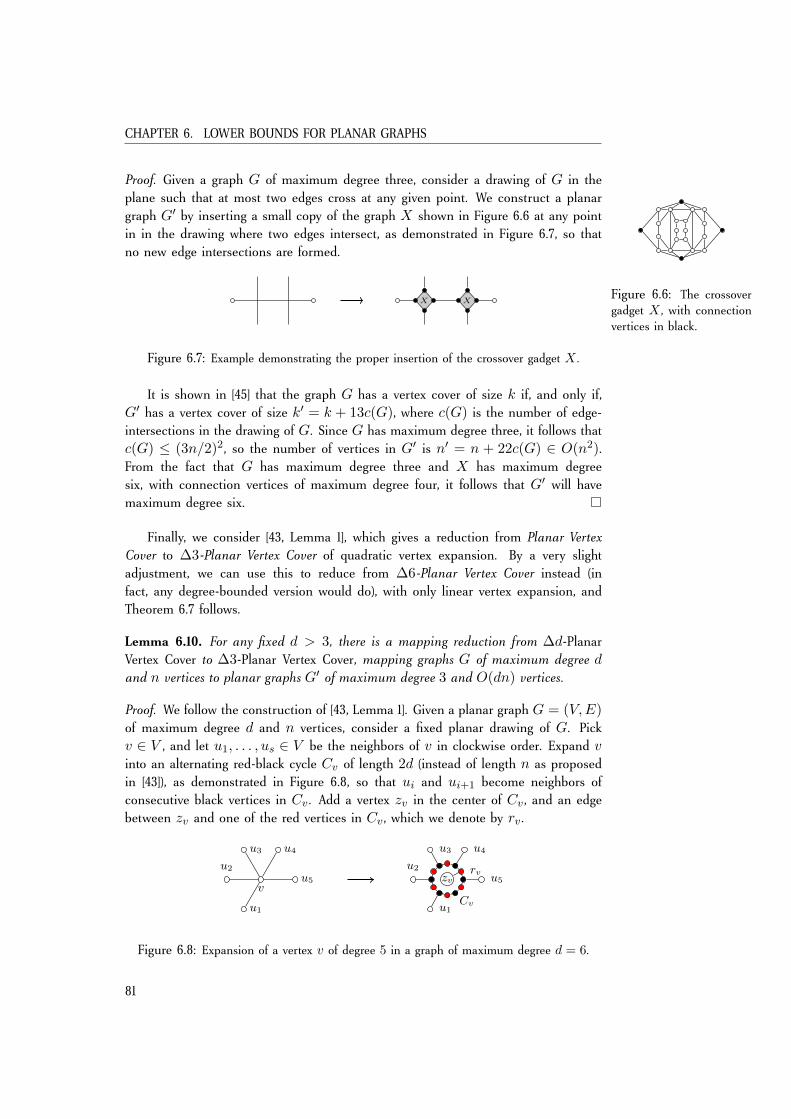
CHAPTER 6. LOWER BOUNDS FOR PLANAR GRAPHS
Proof. Given a graph G of maximum degree three, consider a drawing of G in theplane such that at most two edges cross at any given point. We construct a planargraph G′ by inserting a small copy of the graph X shown in Figure 6.6 at any pointin in the drawing where two edges intersect, as demonstrated in Figure 6.7, so thatno new edge intersections are formed.
Figure 6.6: The crossovergadget X , with connectionvertices in black.
X X
Figure 6.7: Example demonstrating the proper insertion of the crossover gadget X .
It is shown in [45] that the graph G has a vertex cover of size k if, and only if,G′ has a vertex cover of size k′ = k + 13c(G), where c(G) is the number of edge-intersections in the drawing of G. Since G has maximum degree three, it follows thatc(G) ≤ (3n/2)2, so the number of vertices in G′ is n′ = n + 22c(G) ∈ O(n2).From the fact that G has maximum degree three and X has maximum degreesix, with connection vertices of maximum degree four, it follows that G′ will havemaximum degree six.
Finally, we consider [43, Lemma 1], which gives a reduction from Planar VertexCover to ∆3-Planar Vertex Cover of quadratic vertex expansion. By a very slightadjustment, we can use this to reduce from ∆6-Planar Vertex Cover instead (infact, any degree-bounded version would do), with only linear vertex expansion, andTheorem 6.7 follows.
Lemma 6.10. For any fixed d > 3, there is a mapping reduction from ∆d-PlanarVertex Cover to ∆3-Planar Vertex Cover, mapping graphs G of maximum degree dand n vertices to planar graphs G′ of maximum degree 3 and O(dn) vertices.
Proof. We follow the construction of [43, Lemma 1]. Given a planar graph G = (V,E)of maximum degree d and n vertices, consider a fixed planar drawing of G. Pickv ∈ V , and let u1, . . . , us ∈ V be the neighbors of v in clockwise order. Expand vinto an alternating red-black cycle Cv of length 2d (instead of length n as proposedin [43]), as demonstrated in Figure 6.8, so that ui and ui+1 become neighbors ofconsecutive black vertices in Cv . Add a vertex zv in the center of Cv , and an edgebetween zv and one of the red vertices in Cv , which we denote by rv .
vu5
u4u3
u2
u1
zvrv
u5
u4u3
u2
u1Cv
Figure 6.8: Expansion of a vertex v of degree 5 in a graph of maximum degree d = 6.
81
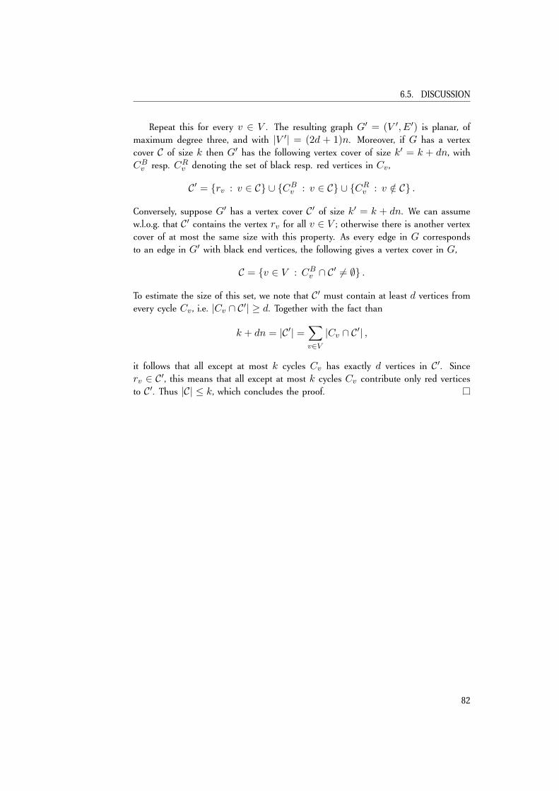
6.5. DISCUSSION
Repeat this for every v ∈ V . The resulting graph G′ = (V ′, E′) is planar, ofmaximum degree three, and with |V ′| = (2d + 1)n. Moreover, if G has a vertexcover C of size k then G′ has the following vertex cover of size k′ = k + dn, withCBv resp. CRv denoting the set of black resp. red vertices in Cv ,
C′ = rv : v ∈ C ∪ CBv : v ∈ C ∪ CRv : v /∈ C .
Conversely, suppose G′ has a vertex cover C′ of size k′ = k + dn. We can assumew.l.o.g. that C′ contains the vertex rv for all v ∈ V ; otherwise there is another vertexcover of at most the same size with this property. As every edge in G correspondsto an edge in G′ with black end vertices, the following gives a vertex cover in G,
C = v ∈ V : CBv ∩ C′ 6= ∅ .
To estimate the size of this set, we note that C′ must contain at least d vertices fromevery cycle Cv , i.e. |Cv ∩ C′| ≥ d. Together with the fact than
k + dn = |C′| =∑v∈V|Cv ∩ C′| ,
it follows that all except at most k cycles Cv has exactly d vertices in C′. Sincerv ∈ C′, this means that all except at most k cycles Cv contribute only red verticesto C′. Thus |C| ≤ k, which concludes the proof.
82
Chapter 7
Open Problems
In Chapter 3, a 2knO(1)-time Monte Carlo algorithm was presented for the K-Cycleproblem. This algorithm can find a shortest solution of given parity, but more thanthat we cannot specify the length of the output. This could be something for futureinvestigations. It would also be interesting to know how close to this time bound adeterministic algorithm could get, as the current best deterministic algorithm is stilldoubly exponential in k10 [62]. Finally, it would of course be nice to find a relevantapplication of this result.
As for the lower bounds in the Tutte plane, the line y = 1, except for the point(1, 1), is still left completely open for simple graphs, and even for multigraphs thebest we have on this line is the exp(Ω( 8
√n))-bound from the planar case. For
simple graphs, only the chromatic line has a lower bound matching the upper boundof exp(O(n)), all other results being of type exp(Ω(n/ logk n)), where k dependson the size expansion of the given reduction. It does not seem unreasonable that thistight bound of the chromatic line could be extended to further points in the plane, orat least that some of the lower bounds could be sharpened by improved reductions.Even more so, the lower bounds of type exp(Ω( k
√n)) reported for the planar case
are for most points very far from the upper bound exp(O(√n)), as discussed in
Section 6.5.
83
84
Appendix A
List of named problems
Below is a list of the statements of computational problems mentioned in the thesis.Other problems are variations or specializations of these problems, according to thefollowing conventions, where Q denotes a given problem:
#Q is the standard counting version of Q (a decision problem),Simple Q is the restriction of Q to simple input graphs,Planar Q is the restriction of Q to planar input graphs,Cubic Q is the restriction of Q to cubic input graphs, and
∆d-Q is the restriction of Q to input graphs of maximum degree d.
3-Coloring
Input: A graph G with n vertices and m edges.Task: Decide whether G has a proper 3-coloring.
3-Sat
Input: A 3-CNF formula ϕ with n variables and m clauses.Task: Decide whether ϕ is satisfiable.
3-Terminal Min-Cut
Input: A graph G = (V,E) with n vertices, m edges, three terminalst1, t2, t3 ∈ V and a number k ∈ N.
Task: Decide whether there is a cut of size k such that t1, t2 and t3are in distinct components.
Clique
Input: A graph G with n vertices, and a number k ∈ N.Task: Decide whether G contains a clique of k vertices.
85
Disjoint Paths
Input: A simple graph G = (V,E) with n vertices, and k vertex pairs(s1, t1), . . . , (sk, tk).
Task: Decide whether G contains k mutually disjoint paths P1, . . . , Pksuch that Pi connects si to ti.
Disjoint Factors
Input: A finite string s of digits from 1, 2, . . . , k.Task: Decide whether there are k disjoint substrings s1, . . . , sk of s
such that si starts and end with the digit i.
Exact Hitting Set
Input: A hypergraph H consisting of m subsets of a finite set V .Task: Decide whether there is a subset S ⊂ V such that
|S ∩ E| = 1 for all E ∈ H.
Hamiltonian Cycle (Path)
Input: A graph G with n vertices and m edges.Task: Decide whether G contains a Hamiltonian cycle (path).
Hitting Set
Input: A hypergraph H consisting of m subsets of a finite set V .Task: Decide whether there is a subset S ⊂ V such that
|S ∩ E| 6= 0 for all E ∈ H.
Independent Set
Input: A graph G with n vertices, and a number k ∈ N.Task: Decide whether G contains an independent set of k vertices.
K-Cycle
Input: A simple graph G = (V,E) with n vertices, and a subsetK ⊆ V ∪ E of size k.
Task: Decide whether G contains a K-cycle.
k-Cycle (-Path)
Input: A graph G with n vertices and m edges, and a number k ∈ N.Task: Decide whether G contains a cycle (path) of length k.
l-K-Hole
Input: A simple graph G = (V,E) with n vertices, a subset K ⊂ Vof size k = (log n)O(1), and a number l ≥ 3.
Task: Decide whether G contains an induced cycle of length l,containing all vertices in K .
86
APPENDIX A. LIST OF NAMED PROBLEMS
Monochrome K-Cycle
Input: An simple, edge-colored graph G = (V,E) with n vertices,and a subset K ⊆ V ∪ E of size k.
Task: Decide whether G contains a monochrome K-cycle.
Steiner Tree
Input: A graph G = (V,E) with n vertices, a set of s terminalst1, . . . , ts ∈ V , and a number k ∈ N.
Task: Decide whether G contains a tree connecting all terminalsand including at most k other vertices.
Tutte(x, y)
Input: A multigraph G with n vertices and m edges.Task: Compute T (G;x, y), as defined in (4.2).
Path Repiability(p)
Input: A graph G = (V,E) with n vertices, m edges,and terminals s, t ∈ V .
Task: Compute Rs,t(G; p), as defined in (6.7).
Vertex Cover
Input: A simple graph G with n vertices, m edges, and k ∈ N.Task: Decide whether G has a vertex cover of size at most k.
87

88

Bibliography
[1] N. Alon, R. Yuster, and U. Zwick. Color-coding. J. ACM, 42(4):844–856, 1995.
[2] M. O. Ball, C. J. Colbourn, and J. S. Provan. Network Reliability. In NetworkModels, volume 7 of Handbooks in operations research and management science,pages 673–762. Elsevier Science, 1995.
[3] R. Barbanchon. On unique graph 3-colorability and parsimonious reductions inthe plane. Theor. Comput. Sci., 319(1–3):455–482, 2004.
[4] E. T. Bax. Inclusion and exclusion algorithm for the Hamiltonian path problem.Inf. Process. Lett., 47(4):203–207, 1993.
[5] R. Bellman. Dynamic programming treatment of the travelling salesman problem.J. ACM, 9(1):61–63, 1962.
[6] A. Björklund. Determinant sums for undirected Hamiltonicity. In Proceedings ofthe 51st Annual IEEE Symposium on Foundations of Computer Science, FOCS 2010,pages 173–182. IEEE Computer Society, 2010.
[7] A. Björklund, T. Husfeldt, P. Kaski, and M. Koivisto. Computing the Tutte polyno-mial in vertex-exponential time. In Proceedings of the 47th annual IEEE Sympo-sium on Foundations of Computer Science, FOCS 2008, pages 677–686, 2008.
[8] A. Björklund, T. Husfeldt, P. Kaski, and M. Koivisto. Narrow sieves for parameter-ized paths and packings. CoRR, abs/1007.1161, 2010.
[9] A. Björklund, T. Husfeldt, and N. Taslaman. Shortest cycle through specifiedelements. In Proceedings of the Twenty-Third Annual ACM-SIAM Symposium onDiscrete Algorithms, SODA 2012, pages 1747–1753. SIAM, 2012.
[10] M. Bläser, H. Dell, and J. A. Makowsky. Complexity of the bollobás-riordanpolynomial. exceptional points and uniform reductions. Theor. Comput. Syst.,46(4):690–706, 2010.
[11] H. L. Bodlaender. Kernelization: New upper and lower bound techniques. InParameterized and Exact Computation, 4th International Workshop, IWPEC 2009,Revised Selected Papers, volume 5917 of Lect. Notes Comput. Sci., pages 17–37,2009.
89
BIBLIOGRAPHY
[12] H. L. Bodlaender, R. G. Downey, M. R. Fellows, and D. Hermelin. On problemswithout polynomial kernels. J. Comput. Syst. Sci., 75(8):423–434, 2009.
[13] H. L. Bodlaender, B. M. P. Jansen, and S. Kratsch. Cross-composition: A newtechnique for kernelization lower bounds. In Proceedings of the 28th InternationalSymposium on Theoretical Aspects of Computer Science, STACS 2011, volume 9 ofLIPIcs, pages 165–176, 2011.
[14] H. L. Bodlaender, S. Thomassé, and A. Yeo. Analysis of data reduction: Transfor-mations give evidence for non-existence of polynomial kernels. Technical report,Department of Information and Computing Sciences, Utrecht University, 2008.
[15] H. L. Bodlaender, S. Thomassé, and A. Yeo. Kernel bounds for disjoint cycles anddisjoint paths. Theor. Comput. Sci., 412(35):4570–4578, 2011.
[16] J. Bondy and U. Murty. Graph Theory, volume 244 of Graduate Texts in Mathe-matics. Springer, 2008.
[17] T. Brylawski. The Tutte polynomial. I. General theory. In Matroid theory andits applications, C.I.M.E. Summer Schools, pages 125–275. C.I.M.E., Ed. Liguori,Napoli & Birkhäuser, 1982.
[18] J. A. Buzacott. A recursive algorithm for finding reliability measures related to theconnection of nodes in a graph. Networks, 10(4):311–327, 1980.
[19] L. Cai and D. Juedes. On the existence of subexponential parameterized algo-rithms. J. Comput. Syst. Sci., 67(4):789–807, 2003.
[20] M. Chudnovsky, G. Cornuéjols, X. Liu, P. D. Seymour, and K. Vuskovic. Recogniz-ing berge graphs. Combinatorica, 25(2):143–186, 2005.
[21] M. Chudnovsky, K. Kawarabayashi, and P. D. Seymour. Detecting even holes. J.Graph Theor., 48(2):85–111, 2005.
[22] M. Chudnovsky, N. Robertson, P. Seymour, and R. Thomas. The strong perfectgraph theorem. Annals of Mathematics, 164:51–229, 2006.
[23] M. Conforti, G. Cornuéjols, A. Kapoor, and K. Vuskovic. Even-hole-free graphspart i: Decomposition theorem. J. Graph Theor., 39(1):6–49, 2002.
[24] M. Conforti, G. Cornuéjols, A. Kapoor, and K. Vuskovic. Even-hole-free graphspart ii: Recognition algorithm. J. Graph Theor., 40(4):238–266, 2002.
[25] H. H. Crapo. The Tutte polynomial. Aequationes Mathematicae, 3:211–229, 1969.
[26] E. Dahlhaus, D. S. Johnson, C. H. Papadimitriou, P. D. Seymour, and M. Yan-nakakis. The complexity of multiterminal cuts. SIAM J. Comput., 23(4):864–894,1994.
90
BIBLIOGRAPHY
[27] N. Dean. Open problems. In Graph Structure Theory: Proceedings of the AMS-IMS-SIAM Joint Summer Research Conference 1991, volume 147 of ContemporaryMathematics, pages 677–688. AMS, 1991.
[28] V. G. Deineko, B. Klinz, and G. J. Woeginger. Exact algorithms for the Hamiltoniancycle problem in planar graphs. Oper. Res. Lett., 34(3):269–274, 2006.
[29] H. Dell, T. Husfeldt, D. Marx, N. Taslaman, and M. Wahlén. Exponential timecomplexity of the permanent and the Tutte polynomial. ACM Trans. Algorithms,to appear.
[30] H. Dell, T. Husfeldt, and M. Wahlén. Exponential time complexity of the perma-nent and the Tutte polynomial. In Automata, Languages and Programming, 37thInternational Colloquium, ICALP 2010, Proceedings, Part I, volume 6198 of Lect.Notes Comput. Sci., pages 426–437. Springer, 2010.
[31] M. Dom, D. Lokshtanov, and S. Saurabh. Incompressibility through colors andids. In Automata, Languages and Programming, 36th International Colloquium,ICALP 2009, Proceedings, Part I, volume 5555 of Lect. Notes Comput. Sci., pages378–389. Springer, 2009.
[32] R. G. Downey and M. R. Fellows. Parameterized Complexity. Springer, 1999.
[33] A. Drucker. New limits to classical and quantum instance compression. InProceedings of the 53rd Annual IEEE Symposium on Foundations of ComputerScience, FOCS 2012, Lect. Notes Comput. Sci. Springer, 2012. To appear.
[34] L. Euler. Solutio problematis ad geometriam situs pertinentis. Commentariiacademiae scientiarum Petropolitanae, 8:128–140, 1741.
[35] M. R. Fellows. The Robertson-Seymour theorems: A survey of applications. InGraphs and Algorithms: Proceedings of the AMS-IMS-SIAM Joint Summer ResearchConference 1989, volume 89 of Contemporary Mathematics, pages 1–18. AMS, 1989.
[36] H. Fleischner and G. J. Woeginger. Detecting cycles through three fixed verticesin a graph. Inf. Process. Lett., 42(1):29–33, 1992.
[37] J. Flum and M. Grohe. Parameterized Complexity Theory. Springer, 2006.
[38] L. Fortnow and R. Santhanam. Infeasibility of instance compression and succinctPCPs for NP. J. Comput. Syst. Sci., 77(1):91–106, 2011.
[39] C. M. Fortuin and P. W. Kasteleyn. Phase transitions in lattice systems withrandom local properties. J. Phys. Soc. Japan, 26(Suppl.):11–14, 1969.
[40] C. M. Fortuin and P. W. Kasteleyn. On the random-cluster model: I. Introductionand relation to other models. Physica, 57(4):536–564, 1972.
91
BIBLIOGRAPHY
[41] S. Fortune, J. E. Hopcroft, and J. Wyllie. The directed subgraph homeomorphismproblem. Theor. Comput. Sci., 10:111–121, 1980.
[42] A. Frank. Packing paths, cuts and circuits - a survey. In Paths, Flows, andVLSI-Layout, volume 9 of Algorithms and Combinatorics, pages 49–100. Springer,1990.
[43] M. R. Garey and D. S. Johnson. The rectilinear Steiner tree problem is NP-complete. SIAM J. Appl. Math., 32:826–834, 1977.
[44] M. R. Garey and D. S. Johnson. Computers and Intractability: A Guide to theTheory of NP-Completeness. W. H. Freeman, 1979.
[45] M. R. Garey, D. S. Johnson, and L. J. Stockmeyer. Some simplified NP-completegraph problems. Theor. Comput. Sci., 1(3):237–267, 1976.
[46] M. R. Garey, D. S. Johnson, and R. E. Tarjan. The planar Hamiltonian circuitproblem is NP-complete. SIAM J. Comput., 5(4):704–714, 1976.
[47] C. Godsil and G. Royle. Algebraic Graph Theory. Graduate Texts in Mathematics.Springer, 2001.
[48] L. A. Goldberg and M. Jerrum. Inapproximability of the Tutte polynomial. Infor-mation and Computation, 206(7):908–929, 2008.
[49] L. A. Goldberg and M. Jerrum. Inapproximability of the Tutte polynomial of aplanar graph. CoRR, abs/0907.1724, 2009.
[50] L. A. Goldberg and M. Jerrum. The complexity of computing the sign of the Tuttepolynomial (and consequent #P-hardness of approximation). CoRR, abs/1202.0313,2012.
[51] R. Haas and M. Hoffmann. Chordless paths through three vertices. Theor. Comput.Sci., 351(3):360–371, 2006.
[52] G. Haggard, D. J. Pearce, and G. Royle. Computing Tutte polynomials. ACM Trans.Math. Softw., 37(3), 2010.
[53] M. Held and R. Karp. A dynamic programming approach to sequencing problems.Journal of the Society for Industrial and Applied Mathematics, 10(1):196–210, 1962.
[54] C. Hoffmann. Exponential time complexity of weighted counting of independentsets. In Proceedings of the 5th International Symposium on Parameterized andExact Complexity, IPEC 2010, volume 6478 of Lect. Notes Comput. Sci., pages180–191. Springer, 2010.
[55] T. Husfeldt. Invitation to algorithmic uses of inclusion-exclusion. In Proceedingsof the 38th international conference on Automata, languages and programming,ICALP 2011, Part II, volume 6756 of Lect. Notes Comput. Sci., pages 42–59. Springer,2011.
92
BIBLIOGRAPHY
[56] T. Husfeldt and N. Taslaman. The exponential time complexity of computingthe probability that a graph is connected. In Proceedings of the 5th InternationalSymposium on Parameterized and Exact Complexity, IPEC 2010, volume 6478 ofLect. Notes Comput. Sci., pages 192–203. Springer, 2010.
[57] R. Impagliazzo, R. Paturi, and F. Zane. Which problems have strongly exponentialcomplexity? J. Comput. Syst. Sci., 63(4):512–530, 2001.
[58] S. Istrail. Statistical mechanics, three-dimensionality and NP-completeness: I.Universality of intractability for the partition function of the Ising model acrossnon-planar lattices. In Proceedings of the 32nd annual ACM Symposium on Theoryof Computing, STOC 2000, pages 87–96. ACM, 2000.
[59] F. Jaeger, D. L. Vertigan, and D. J. Welsh. On the computational complexity ofthe Jones and Tutte polynomials. Math. Proc. Cambridge Philos. Soc., 108(1):35–53,1990.
[60] M. Jerrum and A. Sinclair. Polynomial-time approximation algorithms for theIsing model. SIAM J. Comput., 22(5):1087–1116, 1993.
[61] R. M. Karp. Dynamic programming meets the principle of inclusion and exclusion.Oper. Res. Lett., 1(2):49–51, 1982.
[62] K. Kawarabayashi. An improved algorithm for finding cycles through elements.In Proceedings of Integer Programming and Combinatorial Optimization, 13th In-ternational Conference, IPCO 2008, pages 374–384, 2008.
[63] K. Kawarabayashi and Y. Kobayashi. Algorithms for finding an induced cycle inplanar graphs. Combinatorica, 30(6):715–734, 2010.
[64] K. Kawarabayashi, Z. Li, and B. A. Reed. Recognizing a totally odd K4-subdivision,parity 2-disjoint rooted paths and a parity cycle through specified elements. InProceedings of the Twenty-First Annual ACM-SIAM Symposium on Discrete Algo-rithms, SODA 2010, pages 318–328, 2010.
[65] G. Kirchhoff. Über die Auflösung der Gleichungen, auf welche man bei derUntersuchung der linearen Verteilung galvanischer Ströme geführt wird. Ann.Phys. Chem., 72:497–508, 1847.
[66] D. E. Knuth. Combinatorial Algorithms, Part 1, volume 4A of The Art of ComputerProgramming. Addison-Wesley Professional, 2011.
[67] S. Kohn, A. Gottlieb, and M. Kohn. A generating function approach to the travelingsalesman problem. In ACM ’77 Proceedings of the 1977 annual conference, pages294–300. ACM, 1977.
93
BIBLIOGRAPHY
[68] I. Koutis. Faster algebraic algorithms for path and packing problems. In Automata,Languages and Programming, 35th International Colloquium, ICALP 2008, Pro-ceedings, Part I, volume 5125 of Lect. Notes Comput. Sci., pages 575–586. Springer,2008.
[69] I. Koutis and R. Williams. Limits and applications of group algebras for parame-terized problems. In Automata, Languages and Programming, 36th InternationalColloquium, ICALP 2009, Proceedings, Part I, volume 5555 of Lect. Notes Comput.Sci., pages 653–664. Springer, 2009.
[70] S. Kratsch and M. Wahlström. Preprocessing of min ones problems: A dichotomy.In Automata, Languages and Programming, 37th International Colloquium, ICALP2010, Proceedings, Part I, volume 6198 of Lect. Notes Comput. Sci., pages 653–665.Springer, 2010.
[71] K. Kutzkov. New upper bound for the #3-SAT problem. Inf. Process. Lett., 105(1):1–5,2007.
[72] A. LaPaugh. The subgraph isomorphism problem. Technical report, MassachusettsInstitute of Technology, Laboratory for Computer Science TM 99, 1978.
[73] A. S. LaPaugh and R. L. Rivest. The subgraph homeomorphism problem. J.Comput. Syst. Sci., 20(2):133–149, 1980.
[74] B. Lévêque, D. Y. Lin, F. Maffray, and N. Trotignon. Detecting induced subgraphs.Discrete Appl. Math., 157(17):3540–3551, 2009.
[75] N. Linial. Hard enumeration problems in geometry and combinatorics. SIAM J.Algebra. Discr., 7(2):331–335, 1986.
[76] R. J. Lipton and R. E. Tarjan. A separator theorem for planar graphs. SIAM J.Appl. Math., 36(2):177–189, 1979.
[77] R. J. Lipton and R. E. Tarjan. Applications of a planar separator theorem. SIAM J.Comput., 9(3):615–627, 1980.
[78] D. Lokshtanov. Private communication, February 2012.
[79] L. Lovász. On determinants, matchings, and random algorithms. In Proceedingsof Conference on Fundamentals of Computing Theory, pages 565–574. Akademia-Verlag, 1979.
[80] B. Monien. How to find long paths efficiently. In Analysis and Design of Al-gorithms for Combinatorial Problems, volume 109 of North-Holland MathematicsStudies, pages 239–254. North-Holland, 1985.
[81] L. Onsager. Crystal statistics. I. A two-dimensional model with an order-disordertransition. Phys. Rev., 65:117–149, 1944.
94
BIBLIOGRAPHY
[82] J. Oxley and D. Welsh. The Tutte polynomial and percolation. In Graph Theoryand Related Topics, pages 329–339. Academic Press, 1979.
[83] J. S. Provan. The complexity of reliability computations in planar and acyclicgraphs. SIAM J. Comput., 15(3):694–702, 1986.
[84] J. S. Provan and M. O. Ball. The complexity of counting cuts and of computingthe probability that a graph is connected. SIAM J. Comput., 12(4):777–788, 1983.
[85] N. Robertson and P. D. Seymour. Graph minors .XIII. The disjoint paths problem.J. Comb. Theory, Ser. B, 63(1):65–110, 1995.
[86] J. Scott, T. Ideker, R. M. Karp, and R. Sharan. Efficient algorithms for detectingsignaling pathways in protein interaction networks. J. Comput. Biol., 13(2):133–144,2006.
[87] K. Sekine, H. Imai, and S. Tani. Computing the Tutte polynomial of a graph ofmoderate size. In Algorithms and Computations: 6th International Symposium,ISAAC ’95, Proceedings, volume 1004 of Lect. Notes Comput. Sci., pages 224–233.Springer, 1995.
[88] T. Shlomi, D. Segal, E. Ruppin, and R. Sharan. QPath: a method for queryingpathways in a protein-protein interaction network. BMC Bioinformatics, 7(1):1–9,2006.
[89] A. D. Sokal. The multivariate Tutte polynomial (alias Potts model) for graphsand matroids. In Surveys in Combinatorics, volume 327 of London MathematicalSociety Lecture Note Series, pages 173–226. Cambridge University Press, 2005.
[90] J. W. Suurballe and R. E. Tarjan. A quick method for finding shortest pairs ofdisjoint paths. Networks, 14(2):325–336, 1984.
[91] W. Tutte. The factorization of linear graphs. J. Lond. Math. Soc., 22:459–474, 1947.
[92] W. Tutte. A contribution to the theory of chromatic polynomials. Canad. J. Math.,6:80–91, 1953.
[93] W. Tutte. Graph-polynomials. Advances in Applied Mathematics, 32(1–2):5–9,2004.
[94] D. L. Vertigan. On the Computational Complexity of Tutte, Jones, Homfly andKauffman Invariants. PhD thesis, University of Oxford, 1991.
[95] D. L. Vertigan. The computational complexity of Tutte invariants for planargraphs. SIAM J. Comput., 35(3):690–712, 2005.
[96] H. S. Wilf. Algorithms and complexity. Prentice Hall, 1986.
[97] R. Williams. Finding paths of length k in O*(2k) time. Inf. Process. Lett., 109(6):315–318, 2009.
95


![Exponential Separations in the Energy [2] Complexity of Leader Electionweizhan/files/leaderElectionSTOC.pdf · and for deterministic Leader Election algorithms, there is another exponential](https://img.pdfslide.net/doc/110x75/6014dd53d9794112ea0fff5b/exponential-separations-in-the-energy-2-complexity-of-leader-election-weizhanfilesleaderelectionstocpdf.jpg)