Embed Size (px)
Citation preview

Louisiana State UniversityLSU Digital Commons
LSU Master's Theses Graduate School
2006
Export-led growth in Southern AfricaRamona Sinoha-LopeteLouisiana State University and Agricultural and Mechanical College, [email protected]
Follow this and additional works at: https://digitalcommons.lsu.edu/gradschool_theses
Part of the Agricultural Economics Commons
This Thesis is brought to you for free and open access by the Graduate School at LSU Digital Commons. It has been accepted for inclusion in LSUMaster's Theses by an authorized graduate school editor of LSU Digital Commons. For more information, please contact [email protected].
Recommended CitationSinoha-Lopete, Ramona, "Export-led growth in Southern Africa" (2006). LSU Master's Theses. 1531.https://digitalcommons.lsu.edu/gradschool_theses/1531
EXPORT-LED GROWTH IN SOUTHERN AFRICA
A Thesis
Submitted to the Graduate Faculty of the Louisiana State University and
Agricultural and Mechanical College in Partial Fulfillment of the
requirements for the degree of Master of Science
in
The Department of Agricultural Economics and Agribusiness
By Ramona Sinoha-Lopete
B.S., Louisiana State University, 2004 May 2006

ii
ACKNOWLEDGMENTS
My gratitude goes to Almighty God for granting me the patience, serenity,
wisdom, and knowledge I needed to make this work a success. My sincere gratitude goes
to the University of Equatorial Guinea and to Chevron Equatorial Guinea, which granted
me the opportunity to do postgraduate studies. This work was created through the
unconditional love and moral support of my parents.
My thanks are extended to the Department of Agricultural Economics and
Agribusiness for accepting me into the program. Without the support of my major
professor, Dr. Hector Zapata, this work would not have been completed; therefore, my
gratitude goes to him for his efforts in making this thesis a reality and for contributing to
my understanding and appreciation of econometrics analysis and the topic at hand. I also
want to recognize the collaboration and support I received from my committee members:
• Dr. Roger Hinson, for accepting the responsibility of being part of my
committee, for taking the time to assist, support and advise me on so many
occasions.
• Dr. P. Lynn Kennedy, for collaborating and supporting the preparation of
my thesis.
This work was possible through the efforts of many graduate students in the
Department of Agricultural Economics and Agribusiness, including Dwi Susanto who
helped in my understanding of the basics of time series, and Elizabeth Roule who helped
in making my writing more professional. Thank you to everyone who has contributed to
my success.
iii
TABLE OF CONTENTS ACKNOWLEDGMENTS………………………………………………………………..ii LIST OF TABLES………………………………………………………………………..v LIST OF FIGURES...........................................................................................................vi ABSTRACT……………………………………………………………………………..vii CHAPTER 1. INTRODUCTION…………………………………………………………1
1.1. Problem Definition………………………………………………………………...3 1.2. Justification………………………………………………………………………..4 1.3. Research Objectives……………………………………………………………….5 1.4. Procedure and Data………………………………………………………………..6
1.4.1. Procedure..………………………………………………………………...6 1.4.2. Data..............................................................................................................7
1.5. Thesis Outline……………………………………………………………………..8 CHAPTER 2. LITERATURE REVIEW……………………………………………….....9 2.1. Previous Research on the ELG Hypothesis…………………………………….....9
2.1.1. Cross-Sectional Approach……….………………………………………..9 2.1.2. Time Series Approach……………..……………………………………..11
2.2. Southern Africa Economic Overview…………………………………………....24 CHAPTER 3. METHODOLOGY……………………………………………………….26 3.1. Theoretical Model…..……………………………………………………………26 3.2. Econometric Methods………………………………………………………........27
3.2.1. Unit Root Tests…………………………………………………………..28 3.2.2. Vector Autoregressive Models and Lag Length Selection……………....30 3.2.3. Co-Integration Test: Johansen’s Procedure……………………………...33 3.2.4. Granger-Causality Tests………………………………………………....36
CHAPTER 4. RESULTS AND DISCUSIONS………………………………………….42 4.1. Descriptive Analysis.…………………………………………………………….42 4.2. Econometric Analysis……………………………………………………………47 4.2.1. Unit Root Tests…..……………………………………............................47 4.2.2. VAR Models and Lag Length Selection…………………………………49
4.2.3. Co-Integration Test: Johansen’s……………………………....................51 4.2.4. Granger-Causality Tests of ELG on Bi-Variate Models…………………56
4.3. Comparative Analysis…………………………….……………………………...69 4.3.1. Analysis of the ELG Hypothesis in Southern Africa………………….....69 4.3.2. Botswana………………………………………………………………....75
4.3.3. Lesotho…………………………………………………………………...76 4.3.4. Malawi…………………………………………………………………...77 4.3.5. Mozambique……………………………………………………………..78 4.3.6. Namibia………………………………………………………………......81
iv
4.3.7. South Africa.……………………………………………………………..82 4.3.8. Swaziland…...……………………………………………………………83 4.3.9. Zambia…...………………………………………………………………84 4.3.10. Zimbabwe………………………………………………………………..85
CHAPTER 5. SUMMARY, CONCLUSIONS, LIMITATIONS AND FURTHER RESEARCH……………………………………………………………………………...90 5.1. Summary…………………………...………………………………………….....90 5.2. Conclusions……………………...…………………………………………….....92 5.3. Limitations and Further Research.……………………………………………….93 REFERENCES.………………………………………………………………………….94 APPENDIX A. GRAPHICAL REPRESENTATION FOR SELECTED VARIABLES
FOR SOUTHERN AFRICA (1980-2002)……………………............................99 APPENDIX B. PEARON’S CORRELATION COEFICINET FOR SELLECTED
VARIABLES, SOUTEHRN AFRICA (1980-2002)...........................................105 APPENDIX C. AUGMENTED DICKEY-FULLER AND PHILLIPS-PERRON UNIT
ROOT TESTS, SELECTED VARIABLES (1980-2002)...................................106 APPENDIX D. ARIMA PROCEDURE………………………………………………..115 APPENDIX E. ENGLE-GRANGER’S CO-INTEGRATION PROCEDURE………...119 APPENDIX F. MODELS RESIDUAL DIAGNOSTICS……………………………...121 VITA…………………………………………………………………………………....123

v
LIST OF TABLES 1. Descriptive Statistics for Real GDP, Real Exports, Real Gross Fixed Capital
Formation, and Labor for Southern Africa (1980- 2002)………………………46 2. Optimum Lags on Bi-variate VAR Models for Nine Southern African Countries
(1980-2002)……………………………………………………………………..50 3. Co-Integration Tests on Bi-Variate Models without Exogenous Variables for
Southern Africa (1980-2002)……………………………………….....…………53 4. Co-Integration Tests on Bi-Variate Models with Exogenous Variables for
Southern Africa (1980-2002)…...………………………………………………..54 5. Granger Non-Causality Tests of ELG, Bi-Variate Stationary Models without
Exogenous Variables, Selected Countries (1980-2002)............…………………58 6. Granger Non-Causality Tests of ELG, Bi-Variate Stationary Models with
Exogenous Variables for Swaziland (1980-2002)……..………………………...59 7. Granger Non-Causality Tests of ELG, Bi-Variate Models with No Exogenous
Variables and No Co-integration, Selected Countries, (1980-2002)…………….61 8. Granger Non-Causality Tests of ELG, Bi-Variate Models with Exogenous
Variables and No Co-integration, Selected Countries, (1980-2002)…………….62 9. Granger Non-Causality Tests of ELG, Bi-Variate Models with No Exogenous
Variables and the ECM, Selected Countries (1980-2002)………………..……..65 10. Granger Non-Causality Tests of ELG, Bi-Variate Models with Exogenous
Variables and the ECMX, Selected Countries (1980-2002).....………………….68 11. Tread Policy Reviews for Southern Africa...……………………………………..79 12. Trade Performance Index for Lesotho...…………………………………………88 13. Trade Performance Index for Botswana………………………………………....89 14. Trade Performance Index for Swaziland………………………………………...89

vi
LIST OF FIGURES FIGURE 1. Namibia’s Real GDP, (1980-2002)………………………............................43 FIGURE 2. Namibia’s Real Exports of Goods and Services, (1980-2002).......................43 FIGURE 3. Namibia’s Real Gross Fixed Capital Formation, (1980-2002)......................43 FIGURE 4. Namibia’s Labor Force, (1980-2002).………………………........................43
vii
ABSTRACT
The objective of this thesis was to examine the validity of the Export-Led Growth
(ELG) hypothesis in nine Southern African countries using annual data for the period
1980-2002. The thesis used time series econometric techniques to test for the causal
linkage between exports and economic growth in Southern Africa. Dynamic econometric
models were estimated to test for time series properties: unit root (ADF and PP tests), co-
integration (Johansen’s procedure), and Granger-causality (Likelihood Ratio test-LR).
The results of the unit root tests show that most of the series are stationary in first
differences (series in levels have unit root—I(1)). Co-integration and causality between
exports and economic growth were tested and compared using two types of bi-variate
vector autoregressive models: models without exogenous variables VAR (p), and models
with exogenous variables VARX (p, b). The results of the co-integration tests on both
types of bi-variate models show that all three Granger-causality alternative models fit the
ELG study for Southern Africa (stationary models; integrated but not co-integrated
models; and Error Correction Models). In both types of models, the direction of causation
(unidirectional or bidirectional) between GDP and exports was tested using a SUR
system of equations by computing the LR test. Without exogenous variables, the ELG
hypothesis is found to be valid in Lesotho and Swaziland, and, with exogenous variables,
it is valid in Botswana, Lesotho, and Swaziland, implying that expanding exports can
contribute to economic growth, poverty reduction, and job creation in all three countries.
This research reveals that, even though some countries have adopted export-friendly
policies, the long-term impact of such policies is yet to be observed for most countries.
Keywords: Exports, Economic Growth, VAR (p), Exogenous Variables, VARX (p, b), Co-Integration, ECM, ECMX, SUR, Granger-Causality, Southern Africa
1
CHAPTER 1
INTRODUCTION
The proliferation of trade is in the interest of many countries around the world as
a source of economic growth. The economic argument is that export expansion or export-
led-growth (ELG) leads to efficient allocation of resources resulting from foreign
competition, and to some extent poverty reduction (Hachicha, 2003). Export expansion in
less-developed countries (LDCs) can be used as an instrument of job creation and poverty
reduction. Many countries around the world (e.g., countries in Southern Africa) have
been constantly trying to shift toward the ELG strategy because of the potential benefits
associated with export expansion.
In recent years, some Southern African countries have been enjoying the benefits
associated with openness to the world market (e.g., increases in international oil and
metal prices). Over the last two decades, despite regional, domestic, economic, and social
issues, the economic condition of many Southern African countries has improved. For
instance, in the period 1980-2002, Southern Africa experienced favorable economic
performance. In US$, in 2002, the region’s average real GDP was $23.71 billion, more
than in 1980 ($16 billion). For the period 1980-2002, on average, South Africa’s GDP
was $147.9 billion. Zimbabwe’s GDP was above $6 billion. Zambia, Namibia, Malawi,
and Botswana had a GDP above $3 billion; Mozambique’s GDP was slightly above $2
billion, Swaziland’s GDP was above $1 billion, and Lesotho’s GDP was less than $1
million.
The labor force in the region has also increased. For the period 1980-2002, on
average, South Africa’s labor force was 14 million; Mozambique’s was 7.9 million;
Zimbabwe’s was 4.7 million; Malawi’s was 4.2 million and Zambia’s was 3.3 million.

2
Labor force participation was above 500,000 in Namibia, Botswana, and Lesotho.
Swaziland’s level of labor force was only 290,000.
The amount of capital investment in almost all countries has also increased,
implying that Southern African countries are increasing investment in either human or
physical capital. By improving human capital and increasing domestic productivity, most
Southern African countries are competing with international producers in the production
of goods for which they have a comparative advantage. The value of exports of goods
and services has also increased in almost all Southern African countries. In US$, in 2002,
the value of exports in the region was $6.62 billion, also found to be more than the value
in 1980 ($3.35 billion). In the period 1980-2002, on average, exports of goods and
services were valued at $31.35 billion in South Africa, and approximately $2 billion in
Botswana and Zimbabwe. Exports were almost $1 billion in Zambia and Namibia. For
the same period, Swaziland’s exports were approximately $800 million, in Malawi $416
million and in Mozambique $362 million. The percentage of GDP coming from the
export sector in Southern Africa has been increasing over the years. In 1980, on average,
exports in the region accounted for 40.5% of GDP, and in 2002, this percentage increased
to 45.3%. From 1980 to 2002, exports accounted for more than one third of the region’s
GDP (39%). In most Southern African countries, exports account for more than half of
their GDP. In the period 1980-2002, the percentage of exports contributing to GDP
varied across Southern Africa. Swaziland’s exports were 74.3% of GDP, Botswana’s
57%, Namibia’s 54.2%, Zambia’s 32%, Zimbabwe’s, 27.5%, South Africa’s 27%,
Malawi’s 25%, Lesotho’s 22%, and Mozambique’s 11%. It should be noted, however,
that the value of real GDP, real exports, labor force, and capital in the region vary
considerably depending on each country’s internal characteristics and political situation.

3
Studies have looked at the ELG hypothesis for both developed and less-developed
countries using either time series procedures or cross-sectional approaches. This paper
seeks to investigate how important the role of exports is in the economic growth of
Southern Africa. The study will be centered on a dynamic time series procedure to test
the validity of the ELG hypothesis for Southern Africa, including the countries of
Botswana, Malawi, Mozambique, Namibia, Lesotho, South Africa, Swaziland, Zambia,
and Zimbabwe. The purpose of this study is to answer the following questions: has export
expansion contributed to economic growth in all Southern Africa countries? Does the
empirical evidence support a reverse causal effect from economic growth to exports?
Which countries in Southern Africa are most likely to benefit from export expansion
policies? To test for the causality linkage between exports and economic growth in those
countries, the direction of causation (unidirectional or bidirectional causation) between
GDP and exports will be investigated.
1.1. Problem Definition
In many parts of Africa, poverty and lack of sufficient human capital is an issue of
concern for governments. Despite most African nations’ endowment of natural resources,
some countries have relatively stagnant economic conditions. Some other factors limiting
economic growth in Africa include the presence of weak governance, unstable policy
environments, poor public services, high transportation costs, high levels of
unemployment, insufficient infrastructure, low levels of education, and high rates of
HIV/AIDS infections (i.e., Botswana, Mozambique, Namibia, South Africa, and Zambia)
(Office of the U.S. Global AIDS Coordinator). An important developmental challenge
that continues to affect Sub-Saharan Africa is the presence of high poverty rates. In 2005,
about 43% of people in Sub-Saharan Africa lived in poverty, depending mostly on
4
agriculture to subsist (World Bank, 2005). Over the last two decades, the poverty
situation in Southern Africa has not improved. As for 2002, per capita income in most
Southern African countries did not outpace US$500 (e.g., Mozambique, Zambia, Malawi,
and Zimbabwe). During the 1990s, more than half of Southern Africa’s population lived
under poverty on either $1 or $2 per day (World Bank, 2005).
As Southern Africa’s countries take measures to reduce poverty, one likely
alternative may be the expansion of trade. The momentum generated by recent
agreements through the World Trade Organization provides a unique opportunity to
identify markets for export expansion. However, African nations face trade barriers (high
tariffs, quotas, and subsidies to farmers) from other countries that limit the imports of
African goods. There is little recent empirical evidence studying the relationship between
export expansion and economic growth in Southern Africa. If these countries pursue
policies that promote export expansion, will all countries benefit equally from such
expansion? What does the empirical evidence support, causation from exports to
economic growth or causation from economic growth to exports?
1.2. Justification
The 1980s was a decade of slow or negative growth in per capita GDP, worsening
balance of payments, debt and financial crises, and declining competitiveness for most
African countries (Njikam, 2003). Recently, however, new directions are being taken to
reduce poverty and improve economic conditions in African’s countries. One strategy
taken by many African countries is trade expansion through the encouragement of trade
liberalization with other countries (Anderson, 2004). In Southern Africa, many countries
are initiating economic reforms such as increasing trade within the region (interregional
trade) as well as increasing multi and bilateral trade agreements with other countries
5
outside the region. For many years, scholars have noted that trade liberalization for less-
developed countries can contribute to poverty reduction, economic development, and
growth (Hertel et al., 2001). However, it is uncertain whether expanding exports
ultimately contributes to all Southern African countries’ economic growth. Many studies
have looked at the benefits associated with increasing international trade with
neighboring countries, but few studies have looked at the linkage between exports and
economic growth in Southern Africa. Based on the importance of the ELG hypothesis in
trade and economic literature and the debate regarding its validity for Africa (e.g.,
Southern Africa), a detailed study of this hypothesis is needed for Southern Africa to see
if all countries in the region benefit equally from export-expansion policies. The results
of this analysis are expected to be relevant to Southern Africa policy makers, economists,
and interest groups because promoting growth through export expansion can contribute to
poverty reduction and job creation. The results obtained in this study will be meaningful
to all Southern African countries that rely heavily on their export markets for economic
growth and development. Countries that import products and services from Southern
Africa may also benefit when purchasing goods and services from Southern Africa
countries at favorable prices.
1.3. Research Objectives
The general objective of this thesis is to empirically test the ELG hypothesis for
Southern Africa for the time period 1980-2002.
The specific objectives of this thesis are to:
1. Estimate a dynamic time series econometric model for Southern Africa capturing
the relationship between exports and economic growth,
2. Test for a causal linkage between total exports and economic growth, and

6
3. Conduct a comparative analysis on the ELG hypothesis for Southern African
countries.
1.4. Procedure and Data
1.4.1. Procedure
1.4.1.1. Objective 1
The first objective is to estimate a dynamic time series econometric model for
Southern Africa, capturing the relationship between exports and economic growth (real
GDP growth). To accomplish this objective, neoclassical trade theory will be used to
develop an augmented neoclassical production function. In this model, exports will be
included as an explanatory variable in conjunction with capital and labor. Various Vector
Autoregressive (VAR) models will be estimated. Model specification and selection tests
will be conducted. To select the most appropriate model, two of the most commonly used
model-selection criteria will be used: the Akaike Information Criterion (AIC) and/or the
Schwartz Bayesian criterion (SBC). After the model specification and selection process is
completed, the final model will be estimated using the likelihood-estimation procedure.
For model specification, two tests will be carried out on the series: unit root tests and co-
integration test for long-run equilibrium relationships between the variables. The unit root
tests will be conducted using the Augmented Dickey-Fuller (ADF) and the Phillips-
Perron (PP) tests. Co-integration tests will be conducted using the Johansen’s procedure.
If the variables are found to be integrated but no co-integrated, various VAR in first
differences (VAR-D) will be estimated. If the series are found to be integrated and co-
integrated, various Error Correction Models (ECMs) will be estimated to adjust the series
into their long-run equilibrium conditions.

7
1.4.1.2. Objective 2 The second objective is to test for a causal linkage between total exports and
economic growth in Southern Africa. Granger-causality tests will be used to test for the
ELG and/or growth-led export hypotheses. The significance of the export coefficient in
the real GDP equation will be tested. This test implies that exports in previous periods
predict economic growth better than simply relying on lagged GDP data individually.
The reverse will also be conducted on the real GDP coefficient in the exports equation. If
integration of order one and co-integration are found, the ECM will be used on the co-
integrating vector(s) to test for Granger-causality based on the following null hypotheses:
(1) exports do not cause economic growth in the short run, (2) exports do not cause
economic growth in the long run, and (3) exports do not cause economic growth in either
the short run or the long run. The hypotheses that economic growth does not cause export
in either the short-run or the long-run or overall will also be tested.
1.4.1.3. Objective 3 The third objective is to conduct a comparative analysis on the ELG hypothesis
for Southern Africa. A comparative analysis will be conducted on the results obtained
from objectives one and two for each country separately. The results from the ELG
models, as well as the GDP-led export models, will also be compared. Finally, export
policy implications will be highlighted in a comparative setting.
1.4.2. Data
To carry out this study, time series data for the period 1980-2002 is collected for
Southern African countries where data is available. Nine countries are included in the
analysis: Botswana, Malawi, Mozambique, Namibia, Lesotho, South Africa, Swaziland,
Zambia, and Zimbabwe. The data is obtained from the World Development Indicators

8
CD-ROM (2004) in line with the 1993 System of National Accounts (NSA). The
variables included in the analysis are gross domestic product, total exports of goods and
services, gross fixed capital formation (gross domestic fixed investment) and total labor
force. Gross fixed capital formation is included as a proxy for capital. It is measured as
the total value of a producer’s acquisitions, minus disposals of fixed assets during the
accounting period, plus certain additions to the value of non-produced assets (i.e., subsoil
assets or major improvements in the quantity, quality, or productivity of land) realized by
the productive activity of different institutional groups. All variables (except labor force)
are deflated to 1995 constant US$ (1995=100); labor is measured in million units.
1.5. Thesis Outline
This work is divided into five chapters. Chapter 1 includes the introduction, the
problem definition that leads to the study, the justification of need for the study, the
objectives to be accomplished, and the procedures to be followed. Chapter 2 provides an
extensive literature review on the ELG hypothesis and an overview of Southern Africa
economic conditions. Chapter 3 presents the methodology needed to carry out the study,
including the selected economic theory and the econometric methods to be followed (unit
root tests, co-integration test, and Granger-causality test). Chapter 4 presents the results
obtained from the analysis and the comparative analysis for Southern Africa. Chapter 5
includes the following elements: summary, conclusions, limitations, and the need for
further research on the ELG hypothesis for Southern Africa.

9
CHAPTER 2
LITERATURE REVIEW
2.1. Previous Research on the ELG-Hypothesis
For many years, the impact of exports on economic growth or simply the Export-
Led Growth (ELG) hypothesis has been analyzed in many empirical studies in trade and
economic development (Darrat, 1986). While some studies report causal linkage between
exports and economic growth, others fail to provide evidence to support this relationship.
Recent empirical studies (e.g., Castro-Zuniga in 2004) have investigated the vast amount
of literature covering the issue of ELG in both developed and LDCs using either cross-
sectional or time series approaches.
2.1.1. Cross-Sectional Approach
In cross sectional studies, the ELG hypothesis is tested using either rank
correlation and/or estimating a regression equation where exports are included as an
explanatory variable together with classical inputs of production (capital and labor). In
cross-sectional studies various definitions of exports are considered (i.e., real exports
growth, manufacturing and merchandise exports, exports share of GDP, and the percent
share of changes in exports in GDP). Below is a summary of both types of cross sectional
approach studies.
2.1.1.1. Rank Correlation
With rank correlation, the ELG hypothesis is supported when the correlation
coefficient between exports and output is positive and statistically significant. Limitations
associated with this procedure include the presence of spurious correlation resulting in a
need for minimum development before any association exists; meanwhile, any observed

10
correlation can reflect an underlying relationship through other economic variables (GDP
to exports).
A study using rank correlation was conducted by Findlay (1984) and Krueger
(1985). In this work, the authors tested the ELG hypothesis for four Asian countries
(Hong Kong, Korea, Singapore, and Taiwan) using annual data for the period 1960-1982
(Darrat, 1986). The authors concluded that economic growth in all four countries was
driven by the countries’ export promotion. It was also concluded that higher exports
caused economic growth in all countries. Some limitations of this study included failure
to base conclusions on econometric testing and failure to consider the possibility that
simple correlations may not be appropriate to test for causality since high correlation
between the variables can also be the result of GDP growth resulting in exports.
2.1.1.2. Regression Approach
This approach involves estimating a linear regression model regressing a growth
variable (usually real GDP) against a set of explanatory variables, including exports. The
ELG hypothesis is supported when the coefficient of exports is positive and statistically
significant. By applying this procedure, some scholars agreed that developing countries
with favorable export growth experience a higher rate of economic growth. However,
there are some studies that did not support the idea of higher growth when applying this
procedure, and concluded that in some cases the way countries are grouped needs to be
considered (Giles and Williams, 2000). Some regression studies also concluded that it is
necessary to recognize that ELG changes with time. Some limitations associated with
regression application studies include failure to distinguish between statistical association
and statistical causation. The studies provide little insights about ways the exogenous
variables affect economic growth and the dynamic behavior within countries. They

11
implicitly assume that regression parameters are consistent across countries by not
allowing for differences between countries (e.g., institution, politics, financial structure
and reaction to external shock).
Two of the most commonly reported studies on regression are those conducted by
Ram (1985 and 1987). Ram’s studies represented a transition from the correlation
approach to some judgment of causality that could be achieved through regression
applications. Ram (1985) used the production function regressing real output on capital,
labor, and exports to test the ELG hypothesis on various countries. The countries
included in the analysis varied from developed to less-developed countries It was found
that export performance was important for economic growth for both developed and
LDCs countries. The approach taken in this study was an improvement on previous
studies because it included larger sample LDCs and within the sample, a greater fraction
of low income countries.
2.1.2. Time Series Approach
Time series approaches solve for some of the limitations presented in cross-
sectional studies. In most time series studies, three steps are commonly followed: (1) test
for unit roots in the series (stationary or non-stationary series) using the Augmented
Dickey-Fuller (ADF), and/or Phillip-Perron (PP) tests, (2) test for co-integration, using
Johansen (1988), Johansen and Juselius’s (1990) procedures, and/or Engle-Granger co-
integration approach, and (3) test for causality using the wildly applied causality
approach developed by Granger (1969). In Granger’s causality procedure, there is no
attempt to incorporate economic theory in order to impose any restriction on the
relationship between the variables of interest.
12
Since the 1980s, two of the procedures commonly used in empirical studies have
also been applied to most ELG studies in a dynamic time series setting. These procedures
are the estimation of vector autoregressive models (VAR) developed by Sims (1980)
and/or the structural vector autoregressive models developed by Bernanke, Blanchard and
Watson, and Sims (1986). The two important indicators of the VAR analysis are Impulse
Response Functions (IRFs) and Variance Decompositions (VDCs). These indicators
illustrate the dynamic characteristics of empirical models.
Although time series approaches test for causality between exports and economic
growth using econometric techniques, they still present some problems such as (1)
definition of the information, which some times leads to problems in an ELG study using
Granger-causality tests, (2) aggregation of data, a limitation realized in different findings
for specific countries where researchers have reached mixed conclusions when using
different data sets, and (3) lag-length selection, stationarity, and the presence of
deterministic terms. It is suggested that a researcher selects the appropriate lag-length to
avoid the erroneous conclusions of the Granger-causality test (Castro-Zuniga, 2004).
2.1.2.1. Recent ELG Studies with Time Series Approach
Over the past years, many empirical studies have investigated the validity of the
ELG hypothesis in either a bi-variate or multivariate setting using an augmented
neoclassical production function. Most of these studies used annual, quarterly and/or
monthly data to test for the properties of a time series. The most recent studies have been
reported in Castro-Zuniga’s thesis (2004).
Jung and Marshall (1985) examined the ELG hypothesis testing for causality and
auto-correlation (Box-Pierce statistics to test for general auto-regression on the residuals)
on a bi-variate autoregressive process for the period 1950-1981 for 37 countries. The

13
authors found that the ELG hypothesis was not supported in most of the countries except
for Indonesia, Egypt, Ecuador, and Costa Rica. The export reduction hypothesis was
supported in South Africa, Korea, Pakistan, Israel, Bolivia, and Peru. Unidirectional
causation from growth to exports was found in three countries (Iran, Kenya, and
Thailand), supporting the growth-led export hypothesis. Evidence of growth reducing
export was found in Greece and Israel. The authors did not test for stationarity and co-
integration.
Darrat (1986) re-estimated the ELG hypothesis in four Asian countries (Hong
Kong, Korea, Singapore, and Taiwan) using the same time period employed by Findlay
(1984) and Krueger (1985)—1960-1982. The equations were estimated using the Beach-
Mackinnon maximum-likelihood method correcting for serial correlation. To investigate
the directional causation between exports and economic growth in each country, Granger-
causality tests were used. It was found that exports did not cause economic growth and
economic growth did not generate export in Hong Kong, Korea, and Singapore, implying
that both variables were causally independent. In Taiwan, evidence of unidirectional
causation was found from economic growth to exports. Overall, the author’s empirical
results failed to support the ELG hypothesis in all four countries.
Afxentiou and Serletis (1991) tested the validity of ELG in 16 industrialized
countries using annual data for the period 1950-1985. The countries included in the
analysis were Austria, Belgium, Canada, Denmark, Finland, Germany, Iceland, Ireland,
Japan, Netherlands, Norway, Spain, Sweden, Switzerland, the UK, and the US. Time
series properties were tested and the VAR model was used to test for causality. In the
entire sample, the authors found no evidence of co-integration between GDP and exports.
They found that, in general, only two countries supported either the ELG hypothesis or

14
the growth-led export hypothesis. The ELG hypothesis was only supported in the US and
economic growth-led export was supported in the US and in Norway.
Jin (1995) examined the validity of the ELG hypothesis in four Asian countries
(the four little dragons: Hong Kong, Singapore, South Korea, and Taiwan) using
quarterly data for the period 1973:1-1976:1. A 5-variable VAR model was used. The
relationship between exports and economic growth was tested computing the VDCs, and
the IRF. Co-integration test was also used. Stationary tests on the series were conducted,
and all series were found to be stationary in first differences, thus integrated of order
one—I(1), but co-integrated. The authors found in the VDCs an indication that exports
have significant effect on economic growth in all four countries. It was also found that
growth has an effect on exports in three countries (except in Taiwan). In the IRFs,
bidirectional causation was found from exports to economic growth and from economic
growth to exports in all countries. Thus, the ELG hypothesis was found to be valid in all
four countries.
Jin and Yu (1996) examined the ELG hypothesis in the US in an expanded 6-
variable VAR model using quarterly data for the period 1959:1–1992:3. The study was
considered an extension and synthesis of Sharma et al. (1991) and Marin’s (1992)
studies. The variables included in the model were exports, output, real exchange rates,
foreign output shocks, capital, and labor. The authors stated that increases in foreign
income and depreciation of US currency may raise the nation’s exports. The authors
checked for unit roots and stationarity in the series using the ADF test, and found, in first
differences, the series ( in log-log form) were all stationary—I(1). A co-integration test
was conducted using Engle-Granger’s co-integration procedure and Hansen’s two stage
test, but no evidence of co-integration was found. The authors examined the dynamic

15
effects of one variable on another computing two functions (VDCs and IRFs). In both
functions, they calculated the standard errors using a Monte Carlo Simulation procedure.
It was found that export growth has little effect on economic growth in the US, meaning
that export promotion plays an insignificant role in explaining the movements of GDP
growth in the US. GDP growth was also found to have an insignificant effect on export.
Enriques and Sadorsky (1996) tested the validity of ELG hypothesis for Canada
using annual data for the period 1870-1991. The following variables were included in the
analysis: exports, terms of trade (TOT) and GDP. The authors tested for stationarity (PP
approach), integration (ADF), co-integration (Johansen’s method), and Granger-causality
(VAR model). They found the series to be I(1) and also co-integrated. However, no
evidence supporting the ELG hypothesis was found, but the growth-led export hypothesis
was supported.
Anwer and Sampath (1997) tested the validity of the ELG hypothesis in 97
countries using annual data for the period 1960-1992. They tested for stationarity,
integration, co-integration, and Granger-causality. They found co-integration between
GDP and exports in 36 countries. For the 61 remaining countries, 17 reported no
evidence of co-integration, and 35 reported evidence of causality in at least one direction.
In general, causality from economic growth to exports was found for 30 countries. The
authors found that 29 countries reported positive effects from exports to economic
growth. In 12 countries (out of 30 and out of 29), the positive sign of exports in the GDP
equation and the positive sign of GDP in the exports equation were statistically
insignificant.
Al-Yousif (1997) examined the ELG hypothesis in four Arab Gulf oil producing
countries (Saudi Arabia, Kuwait, United Arab Emirates, and Oman) using annual data for

16
the period 1973-1993. Two models were estimated for each country: one model had the
basic form of the production function and the other was a sectoral model. The author
tested for co-integration and found no long-run relationship between economic growth
and exports in all four countries. Exports were found to be positive and significant in the
economic growth equations in all countries. They found no evidence of serial correlation
when using the Durbin-Watson and Bruesch-Godfrey statistics. Testing for structural
stability of the series using the Farely-Hininch test, the author found that all equations
were structurally stable. A specification test was conducted using White and Hausman’
specification tests and both models were found to be correctly specified.
Shan and Sun (1998) tested the ELG hypothesis for China using monthly data for
the period 1987-1996. This work was distinct from previous studies since it used a 6-
variable VAR model in the production function to avoid specification problems,
controlled for growth of imports to avoid spurious causation results, and tested for
sensibility of causality using different and optimal lag lengths. The Modified Wald test
procedure (MWALD) was used in a Seemingly Unrelated Regression (SUR) that
represents a simplification of the Granger non-causality test. The authors found
bidirectional causation between growth and exports. However, because of the use of the
SUR system, the authors failed to establish short-run or long-run causality between the
variables.
Siddique and Selvanathan (1999) examined the validity of ELG hypothesis for
Malaysia for the period 1966-1996. The variables included in the production function
were total exports, manufacturing exports, and real GDP. The authors tested for
stationarity in the series and the order of integration using ADF test, and found the
variables to be integrated of order one—I(1). A co-integration test was conducted using

17
Engle-Granger’s procedure on the OLS residual series, similar to the Dickey-Fuller (DF)
test, to test the stationarity of the residuals. They found real GDP and exports to be
integrated I(1), but not co-integrated when the lag-lengths were obtained using Akaike’s
(1969) and Schwartz’s (1978) criteria. The authors used the Wald test to test for Granger-
causality and found no evidence supporting the ELG hypothesis but evidence supporting
GDP-led manufacturing export.
Dhawan and Biswal (1999) examined the ELG hypothesis for India using annual
data for the period 1961-1993. They used a VAR model considering the relationship
between real GDP, real exports, and net terms of trade (TOT) for India. All variables
were expressed in natural logarithms. The TOT variable was included in the analysis
because it was believed to have had a significant effect on the country’s exports and
imports prior to 1999. They tested for stationarity applying the unit root tests developed
by Perron (1988). All variables were found to be stationary in first differences—I(1). Co-
integration tests were conducted in a multivariate framework using Johansen (1988) and
Johansen and Juselius (1990) maximum likelihood procedures. They also conducted
additional tests to support the test for co-integration rank, the selection of an appropriate
mode, and stationarity test conditional to co-integration rank. They found evidence of
long-run equilibrium relationships among the variables, which allowed them to test for
the direction of causation using the Error Correction Model (ECM) developed by Engle
and Granger (1987). The results showed short-run and long-run causality between GDP
growth and TOT to export growth. Short-run causality was found from exports to real
GDP growth, indicating that current export promotion strategies led to economic growth
in India. The authors concluded that there is an equilibrium causal relationship between

18
real GDP growth and exports, and a short-run causality from exports to GDP growth.
Thus, promoting exports in India caused economic growth.
Ekanayake (1999) analyzed the causal relationship between exports and economic
growth in eight Asian developing countries using annual data for the period 1960-1997.
The countries included in the analysis were India, Indonesia, Korea, Malaysia, Pakistan,
Philippines, Sri Lanka, and Thailand. The author tested for unit roots in the series, co-
integration between the variables, and causality. The author used these techniques in a bi-
variate model (real exports and real GDP) instead of using them in a multivariate setting
as generally applied in time series studies for their simplicity and importance in time
series analysis. The models were also used to ensure stationarity and provide additional
links through which Granger-causality could be detected when two variables are co-
integrated.
The author tested for unit roots using the ADF test. In first differences, both
variables in all countries where found to be stationary. The optimum lag-length was
estimated using the Akaike final prediction error (FPE) criterion. The author tested for
co-integration (long-run relationship) between the GDP and exports using two co-
integration tests for each country: Engle-Granger’s and Johansen-Juselius’s procedure.
Bidirectional causality was found between exports and economic growth in seven
countries. Evidence of short-run causality was found from economic growth to export
growth in all countries, except in Sri Lanka. Strong evidence of long-run causality
between export and economic growth in all countries was found. Short-run causality was
found between exports and economic growth in two countries (Indonesia and Sri Lanka).
Medina-Smith (2001) tested the ELG hypothesis for Costa Rica for the period
1950-1997 using a Cobb-Douglas production function. The variables included in the

19
analysis were real GDP, real exports, real gross domestic investment, gross fixed capital
formation (a proxy of investment) and population (proxy of labor force). The following
tests were conducted: unit roots (DF and ADF tests), co-integration tests using Co-
integration Regression Durbin-Watson (CRDW), Engle-Granger methods, and
Johansen’s Maximum-likelihood approach. The author found evidence supporting the
ELG hypothesis, implying that exports can explain both the short-run and long-run
economic changes in Costa Rica.
Kónya (2002) re-investigated the possibility of Granger-causality between real
exports and real GDP in 24 OECD1 countries for the period 1960-1997. To make
reasonable comparisons, the data set used in the study was the same as that employed by
Kónya in 2000. The variables included in the study were real GDP, real exports, real imports
of goods and services, and openness, defined as (exports + imports)/GDP. The variable
openness was treated as an auxiliary variable, so the analysis could handle only direct, one-
period-ahead causality between exports and economic growth disregarding the possibility of
indirect causality in the long run. A new panel data approach was used with the Wald test
in Seemingly Unrelated Regressions (SUR), using country specific bootstrap critical
values. The advantages of using this approach include: (1) no requirement for joint
hypotheses for all panel members; it allows for contemporaneous correlation across panel
members, making it possible to exploit the extra information provided by the panel data
setting and (2) apart from the lag structure, the approach does not require any need for pre-
testing. Two different models were used: a bi-variate model (GDP-exports) and a
trivariate model (GDP-exports-openness), both with and without a linear time trend.
1 24 OECD’s countries: Australia, Austria, Belgium, Canada, Denmark, Finland, France, Greece, Iceland, Ireland, Italy, Japan, Korea Rep., Luxembourg, Mexico, Netherlands, New Zealand, Norway, Portugal, Spain, Sweden, Switzerland, UK, and US.

20
However, the focus of the study was oriented on the bi-variate systems. In each situation,
the author focused the analysis on direct causality between exports and GDP. The results
indicated unidirectional causality from exports to GDP in eight countries (Belgium,
Denmark, Iceland, Ireland, Italy, New Zealand, Spain, and Sweden), unidirectional causality
from economic growth to export growth in seven countries (Austria, France, Greece, Japan,
Mexico, Norway, and Portugal), and bidirectional causation between exports and economic
growth in three countries (Canada, Finland, and the Netherlands). No evidence of causality
was found between the variables in Australia, Korea, Luxembourg, Switzerland, the UK, and
the US.
Sentsho (2002) tested the causal relationship between exports and economic
growth in the mining sector in Botswana for the period 1976-1997. The objective of the
study was to see whether revenues derived from the primary exports sector (i.e., mining)
could lead to positive and significant economic growth in Botswana. The author based
the study on evidence from statistical data and an econometric analysis of Botswana’s
economy. To investigate the contribution of exports to Botswana’s economic growth, the
author used two aggregate production function models (APFM). These models assume
that along with the conventional inputs used in the neoclassical production function,
unconventional inputs may be added into the model to identify their contribution to
economic growth. Along with the conventional inputs of production, the following
unconventional variables were included: aggregate exports, primary exports,
manufactured (non-traditional) exports, imports, private sector, government sector,
previous period growth in real GDP, and world GDP. The author estimated the APFMs
through OLS procedures. In the APFM, the author found evidence supporting the
statistical analysis, suggesting that capital, labor force, primary exports, manufactured
21
(nontraditional) exports, imports, government sector, previous period growth in real
GDP, and world GDP are important factors affecting Botswana’s economic growth. The
country is still dependent on primary exports because of the positive impact of traditional
exports and the negative impact of nontraditional exports on the nation’s economic
growth. The results showed that primary export revenues can lead to positive and
significant economic growth in Botswana.
Abdulai and Jaquet (2002) tested the ELG hypothesis for Côte- D’Ivoire. For the
period 1961-1997, the authors examined the short-run and long-run relationship between
economic growth, exports, real investments, and labor force. Time series techniques used
were co-integration and ECM. The authors found evidence of one long-run equilibrium
relationship among all variables. They also found causality, both in the short-run and in
the long-run, flowing from exports to economic growth. Bidirectional causation between
the variables was also found. It was concluded that Côte D’Ivoire’s recent trade reforms
(i.e., promoting domestic investment and recovering international competitiveness)
contribute to export expansion, diversification, and, potentially, future economic growth
in the nation.
Hachicha (2003) tested the dynamic relationship between exports and economic
growth in Tunisia using annual data for the period 1961-1995. The author specified a
system consistent of an export augmented Cobb-Douglas production function, and export
demand supply functions. Unit root tests were conducted for all series using the ADF test,
and the author found all series to be I(1). Co-integration testing was conducted using
Johansen and Juselius’s procedure (1980, 1990). The author estimated the co-integrated
VAR models using either one or two lags, according to the Akaike Information Criterion
(AIC). The variables in the production function and those in the export demand and

22
supply functions were found to be co-integrated. Granger-causality testing was conducted
using the maximum-likelihood estimator to estimate the long-run relationship between
the variables. The results showed a strong association between exports and economic
growth, supporting the ELG hypothesis.
Njikam (2003) tested the ELG hypothesis in 21 Sub-Saharan African2 countries:
The objectives of the study were (1) to test the causal relationship between exports
(agricultural and manufactured) and economic growth, (2) to determine if there is
evidence of such relationships, determine the direction of causality, and (3) to examine
whether the direction of causation is reversed when countries change from import-
substitution strategies (IS) to exports promotion (EP) strategies. The author developed
autoregressive models to determine whether agriculture and manufactured exports cause
economic growth or vise versa in all countries. All variables were in logarithmic form.
Stationary testing on the series was conducted using the ADF test to avoid instantaneous
causation. To determine the optimum lag-length of past information, the minimum final
prediction error (FPE) and Schwarz-Bayesian (SBC) criteria were used. The Hsiao’s
(1979) version (known as the stepwise Granger-causality technique) was used to look at
the direction of causation. The author used the Wald test (WT) and the likelihood ratio
test (LRT) to verify the direction of causation and to test the significance of the restricted
coefficients. It was found that, during the EP period, real GDP and real exports were
stationary in all countries. The optimum lag length for all variables was found to vary
across countries. Unidirectional causation was found from agricultural exports to
economic growth in nine countries (Cameroon, Côte-d’Ivoire, Ghana, Burkina-Faso,
2 21 Sub-Saharan Africa’s countries: Benin, Burkina-Faso, Cameroon, Central Africa Republic, Côte- D’Ivoire, Democratic Republic of Congo (DRC), Gabon, Ghana, Kenya, Madagascar, Malawi, Mali, Nigeria, Niger, Republic of Congo, Senegal, Sierra-Leone, Sudan, Tanzania, Togo, and Zambia.

23
DRC, Madagascar, Malawi, Zambia, and Gabon). Unidirectional causation was found
from manufactured exports to real GDP growth in three countries (Cameroon, Mali, and
Malawi). Unidirectional causation from real GDP to agricultural exports was found in
five countries (Mali, Senegal, Nigeria, Kenya, and Tanzania). The author found
unidirectional causation from real GDP to manufactured exports in six countries (Côte-
D’Ivoire, Ghana, Madagascar, Gabon, Benin, and Togo), implying that total export
growth depends on the economic growth in these countries. Bidirectional causation
between economic growth and agricultural exports was found in three countries
(Burkina-Faso, DRC, and Madagascar), leading to an acceptance of the economic-led
export and the ELG hypotheses in these countries.
Abual-Foul (2004) used annual data for the period 1976-1997 to investigate the
ELG hypothesis in Jordan. The variables included in the analysis were real GDP and real
exports. The author applied Granger-causality tests on Vector Autoregressions (VAR) in
levels (VAR-L), in first differences (VAR-D), and on an Error Correction Model (ECM).
The Akaike’s (1969) criterion of minimum final prediction error (FPE) was used to
determine the optimal lag length for both variables. It was found that the optimum lag
length of the study was 4 years. The use of the optimum lag length helps avoid
misspecifications. To test for causality, the Hsiao’s version of the Granger-causality test
was used. It was found that the parameter estimates of the bi-variate models showed a
positive causal effect of exports on economic growth. In all three bi-variate models,
evidence of unidirectional causation was found from exports to economic growth. Thus,
concluding that the ELG hypothesis is supported in Jordan. To promote faster economic
growth in Jordan, the authors said that government institutions should continue to pursue
their mission of attracting foreign direct investment and increase exports.
24
In all of the above studies (time series approach), the authors saw the need to
move from cross-sectional approach studies to time series approaches because of the
dynamic aspects of time series data. Thus, time series approaches have been widely used
in many recent empirical works analyzing the validity of the ELG in both developed
LDCs.
2.2. Southern Africa Economic Overview
Most recent economic figures from the Economies Intelligence Unit (EIU), the
World Bank, and WTO agree that the economic condition in Africa is now more
favorable than it has been in the past. For instance, Africa’s 2004 economic benefits came
from global expansion gained through higher demand for commodities at higher prices,
improvement in many African nations’ macroeconomic management, reduction of
conflict in some countries (OECD, 2005), rise in official aid, favorable weather
conditions, and the presence of sound macroeconomic policies. Southern Africa also
benefited from the global economic recovery and the overall rise in global commodity
prices (oil and metal prices). The rise in official aid received, most of which was due to
emergency assistance and debt relief, went to good performing countries (Mozambique),
and decreased in some others (Zimbabwe) because of increasing political instability.
Weather conditions were favorable to Southern Africa (Zambia and Malawi, in
particular) since it helped improve agricultural production. However, economic growth in
Southern Africa has not been sufficient to reduce poverty, improve human development
(EIU, 2005), decrease unemployment, and improve the standard of living of many
Southern Africans.
In recent years, in Southern Africa (Angola, Botswana, Lesotho, Malawi,
Mozambique, Namibia, South Africa, Swaziland, Zambia, and Zimbabwe), the role of

25
trade has been considered a way to improve economic development and growth, despite
political instability in some countries (e.g., Zimbabwe). To improve the nations’
economic conditions, many Southern African countries are becoming more open. Trade
in the region has been gaining momentum to boost economic growth and to take
advantage of lower productivity costs in other countries.

26
CHAPTER 3
METHODOLOGY
3.1. Theoretical Model
International trade brings about dynamic impacts critical to a country’s economic
development, including the ability to acquire foreign capital and new technologies. Free
trade with other countries can increase the efficiency of a country’s resource use, and
hence increase the exports of goods in which it has a comparative advantage. However,
when countries—importing countries—impose barriers to trade, the benefits from trade
can be lost. Other important benefits associated with trade include positive export
strategies, such as increases in output, employment and consumption, all of which
increase the demand for a nation’s output (Sentsho, 2002). Trade can also help LDCs by
providing them the foreign exchange necessary for economic development. Countries
that trade are more able to respond to external shocks (weather) than those that do not
trade. In general, external trade generates foreign exchange that contributes to financing
industrialization.
The international trade theory used in this work (Neoclassical Trade Theory) is
based on the principle of comparative advantage of David Ricardo, which states that a
country has a comparative advantage in producing a good if the opportunity cost of
producing that good, in terms of another good, is lower in that country than it is in other
countries. Neoclassical trade theory assumes two factors of production (labor and
capital), equal technology in all countries, perfect competition, and constant returns to
scale, and factor mobility between sectors but not between countries (Appleyard et al.,
2001). In the neoclassical trade theory, trade can take place due to comparative advantage
which is explained through differences in relative factor endowments-factor abundance

27
(Heckscher-Ohlin theorem--HO). The Heckscher-Ohlin theorem states that a country will
produce and export the good whose production makes intensive use of the relatively
abundant factors of production before trade. This country should limit the production and
increase the imports of the good whose production makes intensive use of the expensive
factor of production before trade (Appleyard et al., 2001). In the neoclassical trade
theory, a country will gain from trade whenever its terms of trade (TOT) are different
from its own relative prices in autarky. A country with different Terms of Trade has the
advantage of expanding the production of the factor abundant good, exporting the good
more acceptable in other countries, and importing the good that is relatively more
expensive to produce at home. The neoclassical trade theory will be evaluated in a
neoclassical production function framework incorporating an additional factor of
production (exports) into the production function. Exports are incorporated into the
production function to capture their relationship with aggregate output. The augmented
neoclassical production function is specified as follows:
),,( EXPLKFY = ,
where Y= aggregate output (real GDP), K is capital, L is labor force, and EXP is total
real exports of goods and services. Because of their importance in production, economic
theory says that both capital and labor have positive effects on overall output. Because of
its positive externalities, the ELG hypothesis says that exports must have a positive effect
on aggregate output.
3.2. Econometric Methods
Many economists agree that time series data needs to be analyzed using time
series econometric techniques because of the dynamic effect of the series. To test for the
causal linkage between exports and economic growth in the short-run, in the long-run,

28
and overall, three steps are commonly followed in time series approach studies: (1) test
for unit roots and the order of integration, (2) test for co-integration between the series,
and (3) causality test. In this study, the econometrics procedure to be used follows these
steps mostly taken from Enders (1995). This study will follow all three steps for the
following reasons: to ensure that all variables included in the study are stationary either in
levels or in first differences (unit root tests), to look at the possibility of long-run
relationships between the integrated variables (co-integration test), and to determine the
direction of causation between GDP and exports. Below is a summary of each step.
3.2.1. Unit Root Tests
Although traditional regression models assume that both the dependent and
independent variables are stationary and that the errors have mean zero and constant
variance, a common concern in standard regression models is the presence of unit roots in
the series since most economic time series normally behave with stochastic trends. With
evidence of unit roots, the series are said to be intergraded of order one—I(1), meaning
that they must be modeled in first differences (∆yt = yt - yt-1) to make them stationary. A
time series is stationary if it does not change overtime, which implies that its values have
constant variability. Overall, with evidence of non-stationary variables such as those in
time series analysis, the data might present spurious3 regressions. Thus, unit root tests
account for possible correlation of unit roots in the first differences in the time series.
These tests allow for the presence of a nonzero mean and a deterministic linear time
trend. Two of the wildly used unit root tests will also be applied to this study: the
Augmented Dickey-Fuller (ADF) and Phillips-Perron (PP) tests.
3 A spurious regression has high R2, t-statistics that is significant, but with no significant economic results.
29
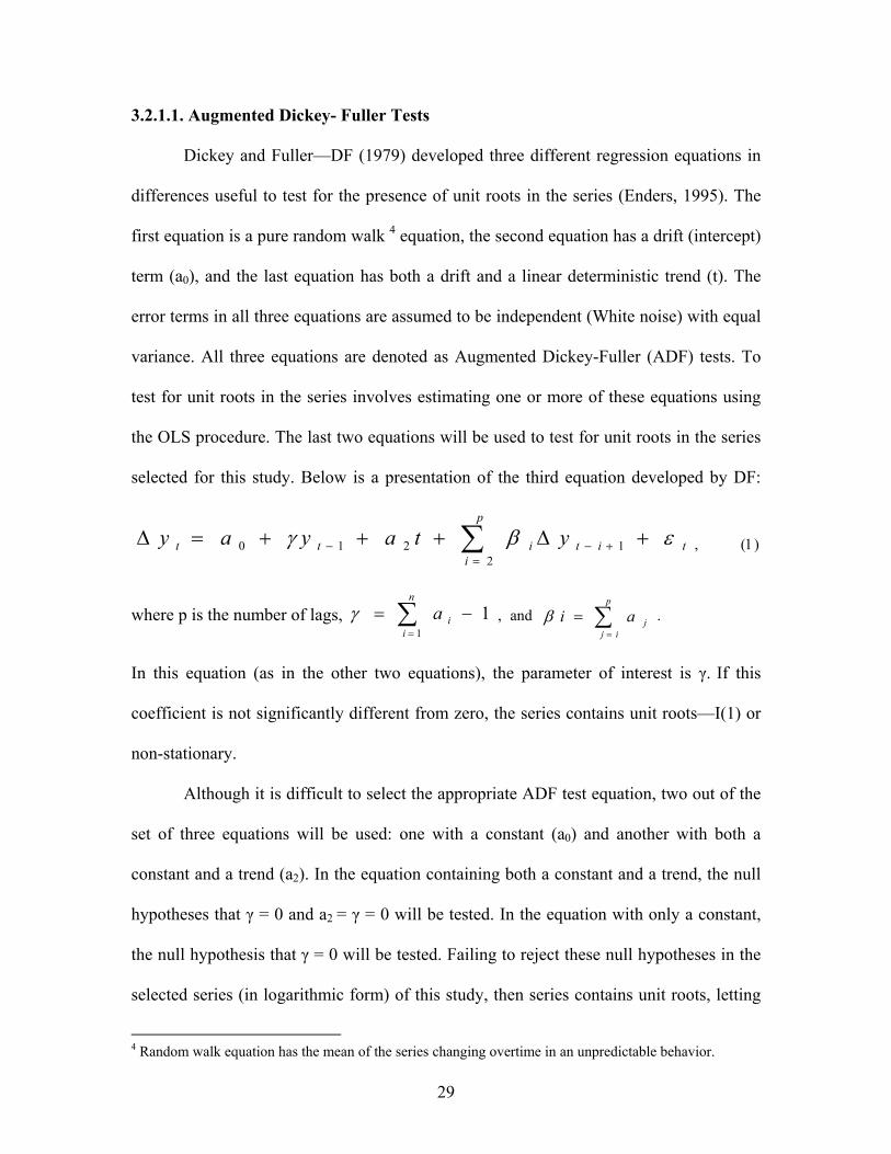
3.2.1.1. Augmented Dickey- Fuller Tests
Dickey and Fuller—DF (1979) developed three different regression equations in
differences useful to test for the presence of unit roots in the series (Enders, 1995). The
first equation is a pure random walk 4 equation, the second equation has a drift (intercept)
term (a0), and the last equation has both a drift and a linear deterministic trend (t). The
error terms in all three equations are assumed to be independent (White noise) with equal
variance. All three equations are denoted as Augmented Dickey-Fuller (ADF) tests. To
test for unit roots in the series involves estimating one or more of these equations using
the OLS procedure. The last two equations will be used to test for unit roots in the series
selected for this study. Below is a presentation of the third equation developed by DF:
t
p
iititt ytayay εβγ +∆+++=∆ ∑
=+−−
21210 , (1)
where p is the number of lags, 11
−= ∑=
n
iiaγ , and ∑
=
=p
ijjaiβ .
In this equation (as in the other two equations), the parameter of interest is γ. If this
coefficient is not significantly different from zero, the series contains unit roots—I(1) or
non-stationary.
Although it is difficult to select the appropriate ADF test equation, two out of the
set of three equations will be used: one with a constant (a0) and another with both a
constant and a trend (a2). In the equation containing both a constant and a trend, the null
hypotheses that γ = 0 and a2 = γ = 0 will be tested. In the equation with only a constant,
the null hypothesis that γ = 0 will be tested. Failing to reject these null hypotheses in the
selected series (in logarithmic form) of this study, then series contains unit roots, letting
4 Random walk equation has the mean of the series changing overtime in an unpredictable behavior.

30
to decide the order of integration I(d). Failing to reject these null hypotheses implies that
the series in levels are non-stationary and they must be modeled in first differences—I(1),
to make them stationary. Rejecting these hypotheses (calculated t-statistics greater than
critical values) implies that the series are stationary and they must be modeled in levels
(actual data) making them I(0).
3.2.1.2. Phillips-Perron Tests
Phillips and Perron (1988) tests for unit roots are a modification and
generalization of DF’s procedures. While DF tests assume that the residuals are
statistically independent (white noise) with constant variance, Phillips-Perron (PP) tests
consider less restriction on the distribution of the disturbance term (Enders, 1995).
Phillips-Perron tests undertake non-parametric correction to account for autocorrelation
present in higher AR order models. The tests assume that the expected value of the error
term is equal to zero, but PP does not require that the error term be serially uncorrelated.
The critical values of PP tests are similar to those given for DF tests.
3.2.2. Vector Autoregressive Models and Lag Length Selection
Two types of bi-variate VAR models will be developed: VAR models with two
endogenous variables (GDP and exports) and VAR models with two endogenous
variables (GDP and exports) and two exogenous variables (gross fixed capital formation
and labor). Bi-variate models without exogenous variables will be developed because of
their simplicity and because they are frequently used in applied works related to ELG, co-
integration, and other studies requiring econometric analysis for pair series (Zapata and
Rambaldi, 1997).
Most of the studies on ELG have treated capital and labor as endogenous
variables or have taken capital and labor out of the analysis to test for the causal

31
relationships between GDP and exports. However, in the neoclassical trade theory capital
and labor are assumed to be inputs of production. Therefore, VAR models with current
exogenous variables will be introduced into the analysis because both exogenous
variables (capital and labor) should be treated as external factors in the production system
(GDP and exports). Bi-variate VAR models with exogenous variables will be introduced
to account for the importance of capital and labor in the production function as inputs and
not as endogenous variables. Developing bi-variate models with exogenous variables will
allow for comparing their results to those that will be obtained from bi-variate models
without exogenous variables. Bi-variate models with exogenous variables are also
introduced to reduce the problems of possible misspecification and multicollineary in the
data selected for all countries. The introduction of bi-variate models with exogenous
variables will be a contribution to ELG and trade literature since little has been done with
exogenous variables when testing the ELG or growth-led export hypotheses. Both types
of models are called bi-variate because of the number of dependent variables in the VAR
models (GDP and exports in both cases). Below, the general forms of both types of bi-
variate VAR models in logarithmic form are illustrated.
Bi-variate VAR models with only endogenous variables with p-lags (L) are
formulated as:
+
+
=
−
−
t
t
t
t
t
t
EXPGDP
LEXPLGDPLEXPLGDP
EXPGDP
2
1
1
1
20
10
)()()()(
εε
ββ
. (2)
And VAR models with exogenous variables with b-lags (B) for each exogenous variable
are formulated as:
+
+
=
−
−
t
t
t
t
t
t
EXPGDP
BLABBGFCFLEXPLGDPBLABBGFCFLEXPLGDP
EXPGDP
2
1
1
1
20
10
)()()()()()()()(
εε
ββ
. (3)

32
Both bi-variate VAR models can be written compactly as:
tptpttt yyyy εββββ +++++= −−− ...22110 , (4)
where yt is a (kx1) vector containing the variables; β10 and β20 are parameters that
represent the intercept terms in each equation; βi represents matrices of coefficients; (L)
is the number of lags entering the autoregressive process since both equations have the
same length; (B) is the number of lags entering the exogenous variables, and ε1t and ε2t
are the error terms assumed to be white noise5 disturbances and uncorrelated.
Overall, the two types of bi-variate VAR models to be determined are the VAR
(p) models (without exogenous variables) and VARX (p, b) models (with exogenous
variables). Several alternative criteria can be used to select the appropriate VAR model
(Yang, 2001) such as the likelihood ratio, the Final Prediction Error (FPE), the Akaike’s
(1969) Information Criterion (AIC), the Schwarz’s (1978) Information Criterion (SIC),
and Hannan and Quinn’s (1978) information criteria (HQ). In all alternatives, the model
that best fits the data is the one that minimizes the Information Criterion Function (ICF)
or simply, the model that minimizes the overall sum of squared residuals or maximizes
the likelihood ratio. However, in this study, the two commonly used model selection
criteria that contribute to the trade off of a reduction in the sum of squared residuals to
form a more parsimonious model will also be used. These selection criteria are the AIC
and the SBC. The final VAR models in this study will be based on the criteria (AIC or
SBC) that minimize the overall sum of squared residuals.
5 White noise process: a sequence of a variable is said to be white noise if the values in the sequence are serially uncorrelated, have mean zero, and variance σ 2
.

33
3.2.3. Co-Integration Test: Johansen’s Procedure
To test for co-integration between GDP and exports, the economic theory
concerning the positive impact of exports, gross fixed capital formation, and labor on
aggregate output will be considered in all nine Southern African countries included in the
study. The econometric specification of this relationship will be captured in various bi-
variate (GDP and exports) models without exogenous variables and various bi-variate
models with exogenous variables, all expressed in logarithmic form. In the bi-variate
models with exogenous variables, gross fixed capital formation and labor will be treated
strictly as exogenous variables. The econometric specification of the relationship between
the variables in both types of bi-variate models is based on augmented neoclassical trade
theory, where all variables are expected to have a positive effect on aggregate output.
Below is a representation of an econometric model of bi-variate form with exogenous
variables:
ttttt LABGFCFEXPY εββββ ++++= lnlnlnln 3210 , (5)
where Y is aggregate output (real GDP), GFCF is real gross fixed capital formation
(gross domestic fixed investment), EXP is total real exports of goods and services, LAB
is labor force, and εt is the stochastic disturbance term (error terms). Econometric theory
assumes that the residual sequences in both types of bi-variate models are stationary, so
that the linear combination of non-stationary series is also stationary.
The concept of co-integration (long-run relationship between variables) was first
introduced by Granger (1969), then extended by Engle-Granger (1987), and Johansen
(1988, 1991, and 1994). This thesis will concentrate on Johansen’s (1988) definition of
co-integration. Johansen’s co-integration procedure will be used to test for the possibility
of at least one co-integrating vector between GDP and exports in all bi-variate models
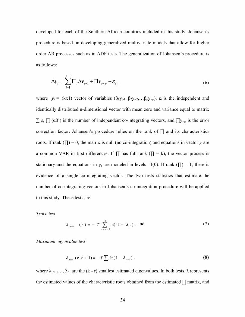
34
developed for each of the Southern African countries included in this study. Johansen’s
procedure is based on developing generalized multivariate models that allow for higher
order AR processes such as in ADF tests. The generalization of Johansen’s procedure is
as follows:
tpt
p
itit yyy ε+Π+∆Π=∆ −
−
=−∑
1
11 , (6)
where yt = (kx1) vector of variables (β1yt-1, β2yt-2,…βpyt-p), εt is the independent and
identically distributed n-dimensional vector with mean zero and variance equal to matrix
∑ ε, ∏ (αβ’) is the number of independent co-integrating vectors, and ∏yt-p is the error
correction factor. Johansen’s procedure relies on the rank of ∏ and its characteristics
roots. If rank (∏) = 0, the matrix is null (no co-integration) and equations in vector yt are
a common VAR in first differences. If ∏ has full rank (∏ = k), the vector process is
stationary and the equations in yt are modeled in levels—I(0). If rank (∏) = 1, there is
evidence of a single co-integrating vector. The two tests statistics that estimate the
number of co-integrating vectors in Johansen’s co-integration procedure will be applied
to this study. These tests are:
Trace test
∑+=
−−=k
riitrace Tr
1
)1ln()( λλ , and (7)
Maximum eigenvalue test
∑ +−−=+ )1ln()1,( 1max rTrr λλ , (8)
where λ r+ 1…, λn are the (k - r) smallest estimated eigenvalues. In both tests, λ represents
the estimated values of the characteristic roots obtained from the estimated ∏ matrix, and

35
T is the number of observations. The trace test attempts to determine the number of co-
integrating vectors between the variables by testing the null hypothesis that r = 0 against
the alternative that r > 0 or r ≤ 1 (r equals the number of co-integrating vectors). The
maximum eigenvalue tests the null hypothesis that the number of co-integrating vectors is
equal to r against the alternative of r+1 co-integrating vectors. If the value of the
likelihood ratio is greater than the critical values, the null hypothesis of zero co-
integrating vectors is rejected in favor of the alternatives.
3.2.3.1. Models Residual Diagnostics
To ensure that the selected lag lengths best fit the selected VAR models, two tests
will be conducted to check that the residuals of all models are white noise (uncorrelated)
and normally distributed. For uncorrelated residuals diagnostic checks, the Portmanteau
residual autocorrelation test (Ljung-Box test) will be used, and for normality testing, the
Jarque-Bera test for normality will be used. The first test examined the null hypothesis
that the residuals are uncorrelated up to some specified number of lags. The second test
investigates the null hypothesis that the residuals of all models are normally distributed.
After selecting the appropriate number of lags entering each VAR model, testing
for co-integration, and checking for white noise and normality on all models’ residuals,
the final VAR models will be estimated using Likelihood estimation procedure. The
optimum number of lags in the VAR models will also be used to fit the models that test
for Granger-causality. The analysis will be concluded testing for Granger-causality on
both types of bi-varaite models with or without evidence of co-integration between the
variables as explained below.

36
3.2.4. Granger-Causality Tests
The final stage of this study is to test for the direction of causation between GDP
and exports on bi-variate models without exogenous variables and bi-variate models with
exogenous variables. Causality testing involves examining whether the lags of one
variable can be included in another equation. To test for the direction of causation
between GDP and exports, the Likelihood Ratio (LR) test developed by Sims in 1980
will be used (Enders, 1995). The LR test statistic is chosen to select the appropriate
number of lags in cross-equation restrictions. The LR has a Chi-square (χ2) distribution
with degrees of freedom equal to the number of restrictions in the system of equations.
The LR is specified as follows:
LR= )log)(log( ∑∑ −− urcT , (9)
where ∑r and ∑u are the variance/covariance matrices of the unrestricted and restricted
system of equations respectively, and c is the maximum number of regressors in the
longest unrestricted equation.
To test for causality between GDP and exports, three Granger-causality
alternative models can be specified on both types of bi-varaite models: VAR in levels,
VAR in first differences, and the ECM. Depending on the results of unit roots and co-
integration tests, the appropriate Granger-causality alternative models that best fit the bi-
variate models developed for each country will be used. Using Seemingly Unrelated
Regressions (SUR), in all three types of VAR models, it will be tested that the parameters
of exports in the GDP equation are jointly equal to zero. It will also be tested that the
parameters of GDP in the export equation are jointly equal to zero.

37
3.2.4.1. VAR in Levels
This model assumes the series to be integrated of order zero (stationary)—I(0) in
levels. When the series in levels are stationary, they can be modeled as VAR in levels
(VAR-L). If the series of this study are stationary in levels, various VAR-L will be
developed for both types of bi-variate models developed for each country. These models
will be used to test for Granger-causality between GDP and exports. The VAR-L with
current exogenous variables will include the following equations for GDP and exports:
11
11
11
11
110 lnlnlnlnln t
b
mmtm
b
nntn
p
jjtj
p
iitit LABGFCFEXPbYbY ερλϕ +++++= ∑∑∑∑
=−
=−
=−
=− , (10)
21
21
21
21
220 lnlnlnlnln t
b
mmtm
b
nnn
p
jjtj
p
iitit LABGFCFYEXPbbEXP ερλϕ +++++= ∑∑∑∑
=−
==−
=−
, (11)
where b10 and b20 are the intercept terms; φ, b, λ, and ρ represent the coefficients of the
variables; and εt1 and εt2 are random disturbances with mean zero, serially uncorrelated
and stationary. The lag length orders of the variables are p (autoregressive process) and b
(exogenous variables).
From equations 10 and 11, the joint hypotheses for Granger non-causality
between GDP and exports, based on stationary variables, state that there is no causation:
From EXP → GDP (Equation 10),
If H0: b11 = b12 =… b1p = 0,
From GDP → EXP (Equation 11),
If H0: φ21 = φ 22 =… φ2p = 0.
The null hypotheses indicate that, with stationary variables, exports do not Granger-cause
economic growth and economic growth does not Granger-cause growth in export.

38
3.2.4.2. VAR in First Differences
The Vector Autoregressive in first differences (VAR-D) assumes that the
variables are integrated of order one—I(1) but not co-integrated. When this is the case,
the differentiated series are modeled as VAR-D. If the variables in this study are I(1) and
not co-integrated (in both types of bi-variate models), Granger-causality will be tested
estimating various VAR-D for both types of bi-varaite models developed for each
country. Below is a representation of GDP and exports equations to be incorporated into
the VAR-D with exogenous variables:
11
11
11
11
110 lnlnlnlnln t
b
mmtm
b
nntn
p
jjtj
p
iitit LABGFCFEXPbYbY ερλϕ +∆+∆+∆+∆+=∆ ∑∑∑∑
=−
=−
=−
=− , (12)
21
21
21
21
220 lnlnlnlnln t
b
mmtm
b
nnn
p
jjtj
p
iitit LABGFCFYEXPbbEXP ερλϕ +∆+∆+∆+∆+=∆ ∑∑∑∑
=−
==−
=− , (13)
where ∆ is the first difference operator and the error terms are white noise.
From Equations 12 and 13, the joint hypotheses for Granger non-causality
between GDP and exports based on no co-integrating relationships indicate that there is
no causation:
From EXP →GDP (Equation 12),
If H0: b11 = b12 =… b1p = 0,
From GDP → EXP (Equation 13),
If H0: φ21 = φ 22 =… φ2p = 0.
The null hypotheses indicate that, with no evidence of co-integration, exports do not
Granger-cause GDP and GDP does not Granger-cause exports.

39
3.2.4.3. Error Correction Model
The Error correction Model (ECM) applies to series that are I(1) and co-integrated
(Engle and Granger, 1987). When this is the case, ECM should be estimated to account
for the variable deviations from equilibrium, a mechanism that brings the economies back
to equilibrium. The ECM is used to estimate the significance of the error term in the co-
integrating vector(s) to see how quickly the series adjust to their long-run equilibrium
condition. To correct for disequilibrium in the co-integrating vector(s), the residuals from
the equilibrium regressions should be used to estimate the ECM (Engle and Granger,
1987). Overall, evidence of co-integration indicates unidirectional or bidirectional
causation between variables (Howard, 2002). If the series in all nine Southern African
countries are I(1) and co-integrated, the co-integrating equations will be expanded
incorporating the error term into the models and testing for the significance of the
adjustment coefficients in each of the co-integrating equations. With evidence of at least
one co-integrating vector (r ≤ k) between GDP and exports in this study, various ECMs
will be determined and specified assuming the presence of deterministic terms (constant).
The deterministic term enters into the ECM via the error correction term. The equations
in both types of VAR models developed in equations 2 and 3 will be transformed into
ECMs with p-lags and with p and b number of lags. Separate ECMs will be estimated,
without exogenous variables (ECMs) and with exogenous variables (ECMXs) in a SUR
system of equations. Below is an illustration of GDP and export equations that fit the
ECMs in both types of bi-variate models:
Bi-variate models without exogenous variables and the ECMs are:

40
111
11
110 lnlnln tt
p
jjtj
p
iitit ZEXPbYbY εχϕ +−∆+∆+=∆ −
=−
=− ∑∑ , (14)
211
21
220 lnlnln tt
p
jjtj
p
iitit ZYEXPbbEXP εδϕ +−∆+∆+=∆ −
=−
=− ∑∑ . (15)
Bi-variate models with exogenous variables and the ECMs (ECMXs) are:
111
11
11
11
110 lnlnlnlnln tt
b
mmtm
b
nntn
p
jjtj
p
iitit ZLABGFCFEXPbYbY εχρλϕ +−∆+∆+∆+∆+=∆ −
=−
=−
=−
=− ∑∑∑∑ , (16)
211
21
21
21
220 lnlnlnlnln tt
b
mmtm
b
nnn
p
jjtj
p
iitit ZLABGFCFYEXPbbEXP εδρλϕ +−∆+∆+∆+∆+=∆ −
=−
==−
=− ∑∑∑∑ , (17)
where (for simplicity) in both types of bi-variate models, Zt-1 is the Error Correction
Term (ECT) representing lagged residuals from the co-integrating relationships. The ECT
represents the disturbance from the equilibrium relationship in co-integrated series; χ and
δ are the long-run adjustment parameters.
From equations 14, 15, 16, and 17, the joint hypotheses for Granger non-causality
based on integrated and co-integrated equations for both types of bi-variate models state
that:
There is no Short-Run Causality:
From EXP → GDP,
If H0: b11 = b12 =… b1p = 0,
From GDP → EXP,
If H0: φ21 = φ 22 = … φ2p = 0.
The null hypotheses, in both types of bi-variate models, state that, in the short-run,
exports do not Granger-cause GDP and GDP does no Granger-cause exports.
There is no Long-Run Causality:
From EXP → GDP,
If H0: χ = 0,
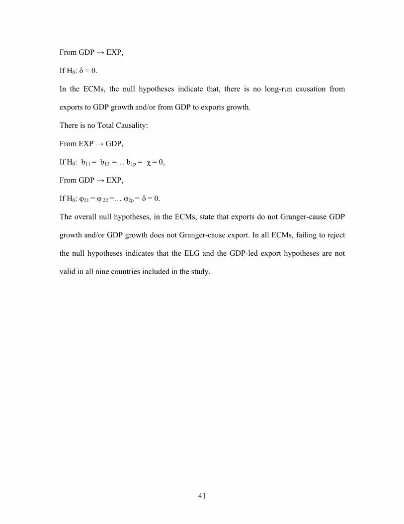
41
From GDP → EXP,
If H0: δ = 0.
In the ECMs, the null hypotheses indicate that, there is no long-run causation from
exports to GDP growth and/or from GDP to exports growth.
There is no Total Causality:
From EXP → GDP,
If H0: b11 = b12 =… b1p = χ = 0,
From GDP → EXP,
If H0: φ21 = φ 22 =… φ2p = δ = 0.
The overall null hypotheses, in the ECMs, state that exports do not Granger-cause GDP
growth and/or GDP growth does not Granger-cause export. In all ECMs, failing to reject
the null hypotheses indicates that the ELG and the GDP-led export hypotheses are not
valid in all nine countries included in the study.

42
CHAPTER 4
RESULTS AND DISCUSSIONS
This chapter presents the results of testing the ELG hypothesis in Southern Africa
for the period 1980-2002. It is composed of three main sections. Section one (section 4.1)
provides a description of the most recent economic performance of all nine Southern
African countries. The next section (section 4.2) presents the results of the econometric
analysis (unit roots, co-integration, and Granger-causality tests) used to test for the causal
linkage between GDP and exports. In the last part of chapter four, a comparative analysis
of the ELG hypothesis and the relevance of the findings for the recent macroeconomic
experience of the countries are discussed.
4.1. Descriptive Analysis
Four macroeconomic indicators (real GDP, real exports of goods and services,
real gross fixed capital formation, and labor force) were used to describe the economic
performance of Southern African countries included in this study. Figures 1 through 4
represent the trend in these four indicators for Namibia for the period 1980-2002. In these
graphs it is seen that all four macroeconomic indicators in Namibia are trending upward.
In real US$, GDP has been steadily rising since the 1980s; exports have remained stable
at approximately $1.5 billion, and gross fixed capital formation started rising in the 1990s
and declined in 2002. Overall, the real value of gross fixed capital formation in Namibia
is trending upward. Labor has also demonstrated a positive trend since the 1980s.
The graphical representation for Botswana, Lesotho, Malawi, Mozambique,
Namibia, South Africa, Swaziland, Zambia, and Zimbabwe are found in Appendix A
(Figures 1 through 32). In Botswana, since 1980, GDP has also been increasing
constantly (Appendix A, Figures 1 through 4). Real exports and labor have also been

43
trending upward over the last 22 years in this country. The highest increase in gross fixed
capital formation was found in 2002. When trying to investigate the reason for the 2002
increase in gross fixed capital formation, it is concluded that it could be due to the
increase in Foreign Direct Investment (FDI) in 2000 that supported the mining industry
of this country.
FIGURE 1. Namibia's Real GDP, (1980-2002)
0
1
2
3
4
5
1980
1982
1984
1986
1988
1990
1992
1994
1996
1998
2000
2002
Period
Mill
ion
US
$
FIGURE 2. Namibia's Real Exports of Goods and Services, (1980-2002)
0
0.5
1
1.5
2
1980
1982
1984
1986
1988
1990
1992
1994
1996
1998
2000
2002
Period
Mill
ion
US
$
FIGURE 3. Namibia's Real Gross Fixed Capital Formation, (1980-2002)
0200400600800
100012001400
1980
1982
1984
1986
1988
1990
1992
1994
1996
1998
2000
2002
Period
Mill
ion
US
$
FIGURE 4. Namibia's Labor Force, (1980-2002)
0
0.2
0.4
0.6
0.8
1
1980
1982
1984
1986
1988
1990
1992
1994
1996
1998
2000
2002
Period
Mill
ion
Figures 5 through 8 represent the trend of all four macroeconomic indicators for
Lesotho, for the same period 1980-2002. The figures reveal continuous increases in GDP,
exports, and labor, while gross fixed capital formation has experienced a decline since the
late-1990s.

44
For Malawi, GDP has constantly been increasing since the 1980s, exports remain
almost the same, gross fixed capital formation has been trending downward since the
1980s, and labor force has been increasing since the 1980s (Appendix A, Figure 9 to 12).
Looking at Mozambique (Appendix A, Figures 13 through 16), the figures show
positive trends in GDP, gross fixed capital formation, and labor; exports remained almost
steady in the 1980s and late 1990s, but it has been increasing since early 2000.
Over the past two decades, South Africa’s GDP has been steadily increasing since
the 1980s; exports remained almost the same from 1980 to early 1990s. From 1980 to
mid-1990s, South Africa experienced a continuous decrease in gross fixed capital
formation; but since 1995, gross fixed capital formation has had a positive trend
(Appendix A, Figures 17 through 20).
Since the late 1980s, GDP has been steadily increasing in Swaziland; exports
have also been increasing in the country; the highest level of gross fixed capital formation
was found in the late 1990s, but it has been declining since then (Appendix A, Figure 21
through 24).
For Zambia, from 1980 to late 1990s, GDP and exports remained very flat.
However, since early 2000s, exports have been increasing. Gross fixed capital formation
had a negative trend from the early 1980s to late 1980s, but it has been increasing since
then (Appendix A, Figures 25 to 28). There is a positive but steady increase in labor.
In Zimbabwe, since the 1980s and late 1990s, the data shows an increase in GDP,
but since early 2000, GDP has been trending downward. The increase in real exports was
also noticeable in the early 1980s and late 1990s. The value of real gross fixed capital
formation has been declining in Zimbabwe. Labor force is trending upward, but at a flat
rate (Appendix A, Figures 29 to 32).

45
In all nine Southern African countries, the data shows that aggregate output (real
GDP), and the value of real exports have been increasing over the years. Table 1
represents a summary of the descriptive statistics for the four macroeconomic indicators
(GDP, exports, gross fixed capital formation, and labor) for the period 1980-2002 for all
nine countries. For the period 1980-2002, the average real GDP for South Africa was
$147.9 billion and for Zimbabwe it was $6.4 billion. Lesotho’s average real GDP was
$800.3 million, and Zambia’s average real GDP was $3.69 billion. In Namibia it was
$3.1 billion; in Malawi it was $1.14 billion, and in Botswana it was $3 billion. In the
same period, Mozambique’s average real GDP was $2.3 billion and Swaziland’s $942.2
million.
On average, total exports in South Africa were $31 billion, above $2 billion in
Botswana and Zimbabwe, and above $1 billion in Zambia and Namibia. Swaziland’s
average real exports were above $800 million and Lesotho’s real exports were only
$189.9 million. Malawi and Mozambique had average real exports of less than $500
million. The value of real exports was slightly above $ 400 million in Malawi and less
than $400 million in Mozambique.
On average, the value of gross fixed capital formation was found in South Africa
to be almost $25 billion. Botswana’s average gross fixed capital formation was $1.18
billion and Zimbabwe’s was $1.1 billion. On average, the value of gross fixed capital
formation in Zambia, Namibia, and Mozambique was above $450 million. In Malawi,
Lesotho, and Swaziland it was less than $400 million for each country.
The number of people in the labor force in Southern Africa is also found to be
increasing but at steady rate since the 1980s. For the period 1980-2002, on average,
South Africa had 14.04 million people in the labor force.

46
Table 1. Descriptive Statistics for Real GDP, Real Exports, Real Gross Fixed Capital Formation, and Labor for Southern Africa (1980-2002).
Country/Variables MEAN STD. DEV. MINIMUM MAXIMUM Botswana GDP 3,982.65 1,763.75 1,393.60 7,022.55 EXP 2,150.21 783.83 752.10 3,505.58 GFCF 1,180.75 725.65 402.83 3,663.41 LAB 0.58 0.12 0.39 0.77 Lesotho GDP 800.33 231.25 498.33 1,151.12 EXP 189.94 134.45 72.84 592.22 GFCF 388.20 148.01 152.73 594.15 LAB 0.64 0.60 0.54 0.74 Malawi GDP 1,302.91 266.77 939.77 1,729.41 EXP 415.86 97.11 261.02 632.00 GFCF 399.13 140.37 206.84 739.60 LAB 4.16 0.62 3.11 5.17 Mozambique GDP 2,299.35 758.00 1,473.30 4,114.78 EXP 361.95 288.06 118.25 1,217.71 GFCF 518.17 386.68 215.07 1,699.13 LAB 7.91 0.84 6.69 9.59 Namibia GDP 3,135.29 681.19 2,405.01 4,372.60 EXP 1,438.75 289.51 973.62 1,824.01 GFCF 668.87 251.77 354.42 1,176.38 LAB 0.61 0.12 0.44 0.82 South Africa GDP 147,946.14 15,705.44 127,410.67 182,280.54 EXP 31,347.88 8,240.27 22,254.59 46,186.68 GFCF 24,982.44 3,327.40 19,602.00 29,479.00 LAB 14.04 2.41 10.35 18.11 Swaziland GDP 1,140.29 368.62 640.34 1,689.78 EXP 866.41 346.78 389.11 1,535.00 GFCF 244.42 73.85 125.86 439.13 LAB 0.29 0.65 0.20 0.40 Zambia GDP 3,697.17 250.66 3,366.00 4,326.00 EXP 1,536.45 233.40 1,230.42 2,157.30 GFCF 497.97 146.44 268.85 769.02 LAB 3.33 0.63 2.40 4.39 Zimbabwe GDP 6,438.80 1,185.36 4,353.86 8,290.92 EXP 2,034.24 913.78 964.65 3,781.49 GFCF 1,111.44 367.44 679.15 1,747.76 LAB 4.74 0.89 3.20 6.06 Note: GDP is Gross Domestic Product; EXP is Exports of Goods and Services; GFCF is Gross Fixed Capital Formation; and LAB is Labor. GDP, EXP, and GFCF are in US Million $ (1995=100); Labor is in Million Units.
47
Mozambique’s labor force was 7.9 million; Zimbabwe’s 4.7 million; Malawi’s
4.2 million and Zambia’s 3.3 million. Labor force participation in Namibia, Botswana,
and Lesotho was above 5,000.
Correlation analysis was done to examine the correlation between the variables
(real GDP, real exports, real gross fixed capital formation, and labor). The results show
strong and positive correlation between the variables in most Southern African countries
(Appendix B, Table 1). At a 5% critical value, strong, positive, and significant correlation
is found between GDP and exports in eight countries (Botswana, Lesotho, Malawi,
Mozambique, Namibia, South Africa, Swaziland, and Zimbabwe). In Zambia, the results
show a positive but not significant correlation between GDP and exports.
The results of the correlation analysis are consistent with the cross-sectional
approach studies (correlation approach), but it should be noted that strong correlation
between the variables does not imply causation from one variable to another (e.g.,
causation from exports to GDP or vise versa).
Therefore, this study examined the direction of causation between real GDP and
real exports. Using time series data (1980-2002), this study tested for three econometric
methods commonly used in recent empirical studies examining the validity of the ELG
for both developed and LDCs: (1) unit roots, (2) co-integration, and (3) Granger-causality
tests. The results of these econometric techniques are summarized in the section that
follows.
4.2. Econometric Analysis
4.2.1. Unit Root Tests
Unit root tests of each series were conduced using the ADF and PP tests. The
critical value applied to both the ADF and PP tests was 10%. In Appendix C (Tables 2

48
through 10), the ADF and PP tests are summarized, both in levels and in first differences.
The tests were performed on all four series (GDP, exports, gross fixed capital formation,
and labor) for Botswana, Lesotho, Malawi, Mozambique, Namibia, South Africa,
Swaziland, Zambia, and Zimbabwe. Tables 2 through 10 (Appendix C) are distributed as
follows: column 1 captures the equations used (with only a constant and with both a
constant and a trend) for both the ADF and PP tests. Column 2 represents the series (in
logarithmic form) and the optimum lags in levels for ADF tests. Column 3 captures all
null hypotheses tested for both the ADF and PP tests, both in levels and in first
differences. In levels, the t-statistics and the decision of accepting or rejecting the null
hypotheses of unit roots in the series are summarized in columns 4 through 7. The second
parts of Tables 2 through 10 summarize the unit root tests in first differences and the
respective decision of accepting or rejecting the non-stationary null hypotheses in first
differences. In levels and in first differences, the optimum lags were obtained using the
AIC. In most Southern African countries, the ADF and PP tests show that most of the
series are non-stationary—I(1) in levels with either a constant or with both a constant and
a trend. For example, in Botswana, the ADF tests shows that, in levels, with either a
constant or with both a constant and a trend, GDP is non-stationary—I(1). In PP test, with
both a constant and a trend, GDP is also non-stationary—I(1). In ADF and PP tests,
exports are non-stationary—I(1) with both a constant and a trend. In both tests, with
either a constant or with both a constant and a trend, gross fixed capital formation
contains unit roots—I(1). Labor, in the ADF test, is non-stationary—I(1) with either a
constant or with both a constant and a trend (Appendix C, Table 2).
To correct for unit root in the series, first differences were taken. The results of
the ADF and PP tests show that, in first differences, (Appendix C, Tables 2 through 10)

49
most of the selected series for Southern African countries are stationary—I(1). For
instance, GDP, exports, and labor, selected for eight countries (Lesotho, Malawi,
Mozambique, Namibia, South Africa, Swaziland, Zambia, and Zimbabwe) are all
stationary—I(1) in first differences, with either a constant or with both a constant and a
trend. In Botswana, the results show that GDP and gross fixed capital formation are non-
stationary in first differences—I(2) with either a constant or with both a constant and a
trend. In Botswana, exports and labor are stationary in first differences—I(1) with either
a constant or with both a constant and a trend.
4.2.2. VAR Models and Lag Length Selection
Two types of bi-variate VAR models were estimated: VAR (p) and VARX (p, b)
models. Because of the sample size, the Akaike Information Criterion (AIC) was used to
estimate the appropriate number of lags entering the VAR (p) and the VARX (p, b)
models specified for all nine Southern African countries included in the analysis. Using
the least squares estimation procedure, it was found that the AIC was minimum for all
VAR (p) and VARX (p, b) models. Thus the final conclusion on the optimum lag lengths
in both types of bi-variate models was based on the minimum AIC. The optimum number
of lags entering the VAR models were determined for the VAR (p) and VARX (p, b)
models developed for eight countries reporting I(1) series: Lesotho, Malawi,
Mozambique, Namibia, South Africa, Swaziland, Zambia, and Zimbabwe. The series for
Botswana had mixed unit root results, two are stationary in first differences (export and
labor) and two (GDP and gross fixed capital formation) are I(2). Thus, GDP (DGDP) and
gross fixed capital formation (DGFCF) were differenced to make all the variables in this
country I(1) to estimate VAR models with equal roots—I(1). Having done so, the VAR
(p) and VARX (p, b) models were also estimated for Botswana with DGDP and DGFCF.

50
This procedure is an attempt to correct for the I(2) problem found in some series in
Botswana. Although limited applied works have looked at mixed integrated series, it was
considered necessary to find ways to solve the mixed integration order problem as oppose
to simply removing a variable(s) or country from the analysis.
Table 2 summarizes the results of the optimum number of lags (based on the AIC)
entering the VAR models. It is found that, in the bi-variate models with no exogenous
variables, the optimum number of lags in the specified VAR (p) model for Botswana is 1.
Each of the VAR (p) model developed for Lesotho, South Africa, and Swaziland is
optimum at 4 lags. Each of the VAR (p) models specified for Malawi, Mozambique,
Namibia, and Zambia is optimum at 2 lags. The VAR (p) developed for Zimbabwe is
optimum at 3 lags.
Table 2. Optimum Lags on Bi-variate VAR Models for Nine Southern African Countries (1980-2002). Countries VAR(p) VARX(p, b) Botswana VAR(1) VARX(1, 4) Lesotho VAR(4) VARX(1, 4) Malawi VAR(2) VARX(1, 4) Mozambique VAR(2) VARX(2, 4) Namibia VAR(2) VARX(1, 4) South Africa VAR(4) VARX(1, 4) Swaziland VAR(4) VARX(4, 2) Zambia VAR(2) VARX(2, 4) Zimbabwe VAR(3) VARX(1, 4)
In the VARX (p, b), where p is the number of lags entering the autoregressive
process of GDP and exports and b the number of lags of each exogenous variable, the
AIC showed that the VARX models is optimum at (1, 4) lags for models developed for
Botswana, Lesotho, Malawi, Namibia, South Africa, and Zimbabwe. The VARX is
optimum at (2, 4) lags for VARX models developed for Mozambique and Zambia. The
VARX model developed for Swaziland is optimum at (4, 2) lags.

51
The optimum number of lags in each autoregressive process (p) estimated for both
types of VAR models developed for each Southern African country was used to test for
co-integration between real GDP and real exports in all nine countries.
4.2.3. Co-Integration Test: Johansen’s
Two preliminary co-integration tests were estimated for countries with I(1) series:
ARIMA process (Box-Jenkins, 1969) and Engle-Granger’s (1987) two step co-integration
procedure. These procedures were conducted to cross-check whether the residual of the
equations (e.g., GDP and exports) are stationary. These co-integration tests were
estimated as preliminary co-integration tests to assess whether the variables in this study
are co-integrated prior to testing for Johansen’s co-integration procedure. Although
ARIMA modeling is no longer popular in this type of research, it was conducted because
it is one of the most intuitive procedures for testing stationarity in time series. ARIMA
procedures were used to examine stationarity in the residuals of co-integrating
regressions for Southern African countries’ models. The Engle-Granger procedure was
used to cross-check the results. Both tests show some degree of co-integration between
the variables since some of the models’ residuals are stationary and uncorrelated (see
Appendix D and E for more detail).
The main focus of this study, however, was to test for co-integration between
GDP and exports in both types of VAR models using the co-integration produce
introduced by Johansen. After testing for unit roots, it is found that, in first differences,
most of the series selected for Lesotho, Malawi, Mozambique, Namibia, South Africa,
Swaziland, Zambia and Zimbabwe are stationary. Thus, co-integration (long-run
relationship) between GDP and exports in bi-variate models without exogenous variables
and with exogenous variables was tested for in these countries. Co-integration between
52
GDP and exports in bi-variate models with no exogenous variables and with exogenous
variables was also tested for Botswana after correcting for the I(2) (DGDP and DGFCF).
The co-integration rank test was applied (trace and maximum eigenvalue tests)
under the restriction that there is no separate drift in the Error Correction Model (ECM),
but a constant that enters only via the ECM. This assumption of the deterministic trend
allowed for the determination of the appropriate ECM to be estimated for all co-
integrating equations in all nine countries. For the trace test, the critical values at 5% is
19.99 when r = 0 and equal to 9.13 when r =1. For the Maximum eigenvalue test, the
critical value at 5% is 15.67 when r = 0 and 9.24 when r = 1. The results of Johansen’s
procedure are summarized in Tables 3 and 4. In Both tables, column 1 represents all nine
countries. Columns 2 captures the null hypotheses (r = 0 and r = 1) of both the trace and
maximum eigenvalue tests. Columns 3 and 4 summarize the trace and maximum
eigenvalue calculated values. The last column represents the co-integrating rank. The last
column also represents the decision of failing to reject or rejecting the null hypothesis of
no co-integration (r = 0). Below is a summary of the results of Johansen’s trace and
maximum eigenvalue tests (under the restriction of deterministic term) in bi-variate
models without exogenous variables and with exogenous variables.
4.2.3.1. Co-Integration Tests on Bi-Variate Models without Exogenous Variables
In Table 3, the results of Johansen’s co-integration tests for at least one co-
integrating vector between real GDP and real exports in all bi-variate models without
exogenous variables developed for all nine countries are summarized. With no exogenous
variables in the bi-variate models, it is found that at a 5% critical level, the trace and the
maximum eigenvalue tests show that, in some countries there exist at least one co-
53
integrating relationship between GDP and exports. For instance, the results show one co-
integrating relationship (vector) between real GDP and real exports in Botswana.
Table 3. Co-Integration Tests on Bi-Variate Models without Exogenous Variables for Southern Africa (1980-2002). Country H_0:
Rank=r
Trace (λtrace)
Max Eigenvalue
(λmax)
RANK
Botswana 0 36.50 29.97 1 6.53 6.53 1 Lesotho 0 36.25 22.15 1 14.11 14.11 2 Malawi 0 26.52 16.78 1 9.75 9.75 2 Mozambique 0 10.58 9.36 0 1 1.22 1.22 Namibia 0 21.57 13.64 1 7.93 7.93 1 South Africa 0 40.61 36.17 1 4.44 4.44 1 Swaziland 0 52.55 34.64 1 17.90 17.90 2 Zambia 0 5.29 3.3 0 1 1.99 1.99 Zimbabwe 0 13.91 10.22 0 1 3.70 3.70 Note: H_0 for both tests is rank=r; alternative hypotheses: trace: H_1: rank>r; max eigenvalue H_1: rank=r+1. At 5% critical value: Trace: for r=0 is 19.99; for r=1 is 9.13. Max eigen: for r=0 is 15.67, for r=1 is 9.24.
Overall, in bi-variate models with no exogenous variables, one co-integrating
relationship (vector) is found between real GDP and exports in three countries
(Botswana, Namibia, and South Africa). Two co-integrating relationships between real
GDP and exports are found in three countries (Lesotho, Malawi, and Swaziland),
indicating that the vectors developed for these countries are full ranked (k). A full rank
vector indicates that the variables in the VAR models are stationary in levels—I(0). No
co-integrating relationship between the GDP and exports is found in three countries
(Mozambique, Zambia, and Zimbabwe).

54
4.2.3.2. Co-Integration Tests on Bi-Variate Models with Exogenous Variables
Co-integration (long-run relationship) between real GDP and real exports was
also conducted on bi-variate models with exogenous variables (gross fixed capital
formation and labor). Table 4 summarizes the results of Johansen’s trace and maximum
eigenvalue tests for models with exogenous variables. With exogenous variables in the
bi-variate models, it is found that, at a 5% critical level, the trace and the maximum
eigenvalue tests show at least one co-integrating relationship between GDP and exports
in Botswana, Lesotho, Malawi, South Africa, and Swaziland.
Table 4. Co-Integration Tests on Bi-Variate Models with Exogenous Variable for Southern Africa (1980-2002). Country/ Null Hypothesis
H_0:
Rank=r
Trace (λtrace)
Max Eigenvalue
(λmax)
RANK
Botswana 0 36.50 29.97 1 6.53 6.53 1 Lesotho 0 23.48 17.46 1 6.03 6.03 1 Malawi 0 23.23 19.19 1 4.03 4.03 1 Mozambique 0 10.58 9.36 0 1 1.22 1.22 Namibia 0 28.24 21.94 1 6.30 6.30 1 South Africa 0 25.20 17.48 1 7.72 7.72 1 Swaziland 0 52.55 34.64 1 17.90 17.90 2 Zambia 0 11.18 9.16 0 1 2.02 20.2 Zimbabwe 0 16.77 10.50 0 1 6.28 6.28 Note: H_0 for both tests is rank=r; alternative hypotheses: trace: H_1: rank>r; max eigenvalue H_1: rank=r+1. At 5% critical value: Trace: for r=0 is 19.99; for r=1 is 9.13. Max eigenvalue: for r=0 is 15.67, for r=1 is 9.24.
Overall, when treating gross fixed capital formation and labor as exogenous
variables and real GDP and real exports as dependent variables, the results of trace and
maximum eigenvalue tests show evidence of one co-integrating relationship in five
55
countries (Botswana, Lesotho, Malawi, Namibia, and South Africa). Two co-integrating
relationships are found in Swaziland, indicating that the vector is full ranked, implying
that a VARX (p, b) model in levels is the appropriate model. No evidence of co-
integration is found in three countries (Mozambique, Zambia, and Zimbabwe).
4.2.3.3. Models Residual Diagnostics
Residual diagnostic checks were conducted on all models using Portmanteau and
Jarque-Bera normality tests (see Appendix F, Tables 12-15). In the bi-variate models with
no exogenous variables, the results of Portmanteau test shows that all of the models’
residuals, up to specified number of lags (maximum of 4 lags), are uncorrelated in all
countries (Appendix F, Table 12), and the results of the normality test show that all bi-
variate models’ residuals in all countries (except DGDP6 for Botswana) are normally
distributed (Appendix F, Table 13) at 5% and 10% critical values. The residuals in
Lesotho, South Africa, and Swaziland are not white noise at 5 lags; increasing7 the lag
length did not correct for residual cross-correlation in those countries. Therefore, it is
assumed that the residuals are white noise in Lesotho, South Africa and Swaziland at 4
lags.
In VARX (p, b) models, Portmanteau tests show that most of the models residuals
are uncorrelated up to a certain number of lags (Appendix F, Table 14) at 5% and 10%
critical values in all countries. Except for South Africa and Swaziland, the residuals are
found to be white noise for all countries. It is assumed that the models residuals
developed for South Africa and Swaziland are white noise at 1 lag (South Africa) and 4
lags (Swaziland). Jarque-Bera normality tests show that all of the models residuals with
6 DGDP is first differences of GDP and DGFCF is the first difference of Gross fixed capital formation. 7 The sample size used does not allow increase in lags (22 observations).
56
exogenous variables are normally distributed at 5% and 10% critical values (Appendix F,
Table 15).
4.2.4. Granger-Causality Tests of ELG on Bi-Variate Models
After testing for co-integration between GDP and exports in all nine countries, the
co-integration results showed that all three Granger-causality alternative VAR models
(causality on stationary variables—VAR-L, causality on integrated but not co-integrated
variables—VAR-D, and causality on integrated and co-integrated series—ECMs) are
applicable to both types of bi-variate VAR models developed in this study.
Therefore, various Seemingly Unrelated Regressions (SUR) systems of equations
were estimated to test for the causal linkage between real GDP and real exports. The
same number of lags in the specified VAR (p) and VARX (p, b) models were used to
estimate the SUR models in levels, in first differences, and estimation of various ECMs
for all nine countries. The SUR models were developed to estimate unrestricted and
restricted models from which to test for Granger non-causality of ELG and GDP-led
export hypotheses.
The Likelihood Ratio (LR) test was used to determine the direction of causation
(unidirectional and/or bidirectional causation) between GDP and exports on all SUR
models developed for all countries. The selected critical value applied to the SUR models
and the LR test is 5%.
Below is a summary of the results of the Granger non-causality test of the ELG
and GDP-led export hypotheses for both types of bi-variate models estimating all three
alternative Granger-causality VAR models. The decision of failing to reject the null
hypotheses of Granger non-causality (NO) is common for both types of bi-variate models
developed for all countries. Because the purpose of this study is to examine the validity
57
of the ELG hypothesis in all Southern African countries, the acceptance of the alternative
hypotheses of Granger-causality (YES) is also reported.
4.2.4.1. Granger Non-Causality Tests on Full Ranked Bi-Variate Models
Granger non-causality tests of ELG and GDP-led export on stationary models
(full rank, r = 2) was found to be applicable to both types of estimated bi-variate models
in some countries. Below is a summary of the results of the Granger non-causality tests
on each type of bi-variate stationary models for some countries.
4.2.4.1.1. Granger Non-Causality Tests without Exogenous Variables
The co-integration tests results without exogenous variables showed that the VAR
models developed for Lesotho, Malawi, and Swaziland are all full ranked. For this, SUR
systems of equations were estimated in levels for Lesotho, Malawi, and Swaziland using
the same number of lags in the estimated VAR (p) models.
On the SUR models, the direction of causation between GDP and exports was
tested calculating the LR test and its respective chi-square statistics. The results of the LR
test and the chi-square are summarized in Table 5. Column 1 presents the direction to
causation from one variable to another for each country. The last column of table 5
captures the decision to fail to reject the null hypothesis of Granger non-causality. Below
is a summary presentation of the results of the Granger non-causality of ELG and GDP-
led export hypotheses for stationary bi-variate models without exogenous variables for
Lesotho, Malawi, and Swaziland.
4.2.4.1.1.1. Causality from Exports to GDP
In Lesotho and Swaziland, at a 5% critical value, the results of the LR test show
that exports cause real GDP, allowing for an acceptance of the ELG hypothesis in these
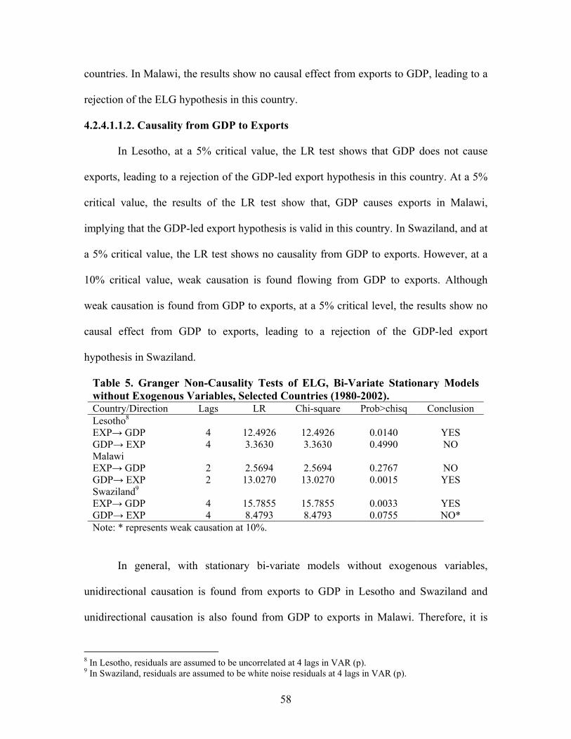
58
countries. In Malawi, the results show no causal effect from exports to GDP, leading to a
rejection of the ELG hypothesis in this country.
4.2.4.1.1.2. Causality from GDP to Exports
In Lesotho, at a 5% critical value, the LR test shows that GDP does not cause
exports, leading to a rejection of the GDP-led export hypothesis in this country. At a 5%
critical value, the results of the LR test show that, GDP causes exports in Malawi,
implying that the GDP-led export hypothesis is valid in this country. In Swaziland, and at
a 5% critical value, the LR test shows no causality from GDP to exports. However, at a
10% critical value, weak causation is found flowing from GDP to exports. Although
weak causation is found from GDP to exports, at a 5% critical level, the results show no
causal effect from GDP to exports, leading to a rejection of the GDP-led export
hypothesis in Swaziland.
Table 5. Granger Non-Causality Tests of ELG, Bi-Variate Stationary Models without Exogenous Variables, Selected Countries (1980-2002). Country/Direction Lags LR Chi-square Prob>chisq Conclusion Lesotho8 EXP→ GDP 4 12.4926 12.4926 0.0140 YES GDP→ EXP 4 3.3630 3.3630 0.4990 NO Malawi EXP→ GDP 2 2.5694 2.5694 0.2767 NO GDP→ EXP 2 13.0270 13.0270 0.0015 YES Swaziland9 EXP→ GDP 4 15.7855 15.7855 0.0033 YES GDP→ EXP 4 8.4793 8.4793 0.0755 NO* Note: * represents weak causation at 10%.
In general, with stationary bi-variate models without exogenous variables,
unidirectional causation is found from exports to GDP in Lesotho and Swaziland and
unidirectional causation is also found from GDP to exports in Malawi. Therefore, it is
8 In Lesotho, residuals are assumed to be uncorrelated at 4 lags in VAR (p). 9 In Swaziland, residuals are assumed to be white noise residuals at 4 lags in VAR (p).

59
concluded that the ELG is valid in two countries (Lesotho and Swaziland) and the GDP-
led export is only valid in Malawi. However, at a 10% critical value, weak causation is
found from GDP to exports in Swaziland.
4.2.4.1.2. Granger Non-Causality Tests with Exogenous Variables
Including exogenous variables into the bi-variate models, it was found only the
VARX model developed for Swaziland is full ranked. Thus, using the same number of
lags in the VARX (p, b) model developed for Swaziland, SUR systems of equations were
estimated in levels for real GDP and exports; and the direction of causation between GDP
and exports was also tested. Table 6 summarizes the LR test for Granger non-causality of
ELG and GDP-led export in Swaziland. Below is a summary of Granger non-causality of
ELG and GDP-led export hypotheses for stationary VARX models developed for
Swaziland.
4.2.4.1.2.1. Causality from Exports to GDP
At a 5% critical value, the results show that, exports cause GDP, allowing for an
acceptance of the ELG hypothesis in Swaziland.
4.2.4.1.2.2. Causality from GDP to Exports
No causation is found from GDP to exports, at a 5% critical value, leading to a
rejection of the GDP-led export hypothesis in Swaziland. Overall, unidirectional
causation is found from exports to GDP in this country.
10 In Swaziland (exogenous variables), the residuals are assumed to be white noise at 4 lags.
Table 6. Granger Non-Causality Tests of ELG, Bi-Variate Stationary Models with Exogenous Variables for Swaziland10 (1980-2002). Direction Model Lags LR Chi-square Prob>chisq Conclusion EXP→ GDP VARX(p, b) (4, 2) 10.302 10.3017 0.0356 YES GDP→ EXP VARX(p, b) (4, 2) 2.4472 2.4472 0.6541 NO Note: p number of lags in the autoregressive process; b number of lags of exogenous variables.

60
4.2.4.2. Granger Non-Causality Tests on VAR Models in First Differences
Granger non-causality test of ELG on no-cointegrating equations (VAR-D) was
conducted on both types of estimated bi-variate models developed for some countries.
Below is a summary of the results of Granger non-causality tests of ELG and GDP-led
export on both types of bi-variate models in first differences for some countries.
4.2.4.2.1. Granger Non-Causality Tests on VAR-D without Exogenous Variables
Various SUR systems of equations in first differences were estimated to test for
the direction of causation between real GDP and real exports in Mozambique, Zambia,
and Zimbabwe. The optimum number of lags the SUR models was obtained from the
estimated VAR (p) models.
Table 7 summarizes the Granger non-causality test of ELG and GDP-led export in
Mozambique, Zambia, and Zimbabwe by computing the LR tests in each equation
developed for each country. Column 1 of Table 7 captures the direction of causation
(unidirectional or bidirectional causation between GDP and exports) of each variable in
each country. The distribution of Table 7 is similar to that presented in Table 5. Below is
a summary of the result of the Granger non-causality of ELG and GDP-led export
hypotheses on bi-variate models without exogenous variables and no co-integrating
relationship for Mozambique, Zambia, and Zimbabwe.
4.2.4.2.1.1. Causality from Exports to GDP
At a 5% critical value, the results show that, exports do not cause GDP in
Mozambique, Zambia, and Zimbabwe, allowing for a rejection of the ELG hypothesis in
all three countries.

61
4.2.4.2.1.2. Causality from GDP to Exports
At a 5% critical value, the results of the LR test also show no causal effect
flowing from GDP to exports in all three countries (Mozambique, Zambia, and
Zimbabwe). However, at a 10% critical value, weak causation is found from GDP to
exports in Zambia.
In conclusion, in bi-variate models without exogenous variables, weak causation
is found from GDP to exports in Zambia. No unidirectional and/or bidirectional causation
is found between GDP and exports in Mozambique, Zambia, and Zimbabwe. With these
results, it is conclude that the ELG and the GDP-led export hypotheses are not valid in all
three countries reporting no co-integrating relationship between GDP and exports.
Table 7. Granger Non-Causality Tests of ELG, Bi-Variate Models with No Exogenous Variables and No Co-Integration, Selected Countries (1980-2002). Direction/country Lags LR Chi-square Prob>chisq Conclusion Mozambique EXP→ GDP 2 1.25131 1.25131 0.5349 NO GDP→ EXP 2 0.8268 0.8268 0.6661 NO Zambia EXP→ GDP 2 0.20478 0.20478 0.9026 NO GDP→ EXP 2 5.9022 5.9022 0.0523 NO* Zimbabwe EXP→ GDP 3 0.6735 0.6735 0.8794 NO GDP→ EXP 3 0.2084 0.2084 0.9762 NO Note: Lags are the number of lags in the VAR (p) models with no exogenous variables; * indicates weak causation.
4.2.4.2.2. Granger Non-Causality Tests on VAR-D with Exogenous Variables
Incorporating exogenous variables into the models, no co-integrating relationship
was found between GDP and exports in Mozambique, Zamia, and Zimbabwe. Thus,
various SUR systems of equations in first differences were estimated to test for Granger-
non causality of ELG and GDP-led export hypotheses for all three countries. The same
number of lags in the estimated VARX models developed for each country was used.

62
Table 8 summarizes the Granger non-causality tests of the ELG and GDP-led export
hypotheses for no co-integrating equations. The description of Table 8 is similar to that
presented in Table 6. Below is a summary of the results of the Granger non-causality tests
on bi-variate models with exogenous variables and no co-integrating relationship for
Mozambique, Zambia, and Zimbabwe.
4.2.4.2.2.1. Causality from Exports to GDP
In Mozambique, Zambia, and Zimbabwe, at a 5% critical value, the results show
that exports do not cause GDP in any of these countries, leading to a rejection of the ELG
hypothesis in all three countries.
Table 8. Granger Non-Causality Tests of ELG, Bi-Variate Models with Exogenous Variables and No Co-Integration, Selected Countries (1980-2002). Country/Direction Model Lags LR Chi-
square Prob>chisq Conclusion
Mozambique EXP→ GDP VARX(p, b) (2, 4) 0.11401 0.11401 0.9446 NO GDP→ EXP VARX(p, b) (2, 4) 1.5194 1.5194 0.4678 NO Zambia EXP→ GDP VARX(p, b) (2, 4) 0.0102 0.0102 0.9195 NO GDP→ EXP VARX(p, b) (2, 4) 0.00071 0.00071 0.9790 NO Zimbabwe11 EXP→ GDP VARX(p, b) (1 4) 1.7605 1.7605 0.1846 NO GDP→ EXP VARX(p, b) (1 4) 1.4226 1.4226 0.2330 NO
4.2.4.2.2.2. Causality from GDP to Exports
At a 5% critical value, no causal effect is found from GDP to exports in
Mozambique, Zambia, and Zimbabwe, thus, leading to a rejection of the GDP-led export
hypothesis in all three countries. Overall, in bi-variate models with exogenous variables
and no co-integrating relationships, no unidirectional and/or bidirectional causation is
found between GDP and exports. Thus, it is concluded that the ELG and the GDP-led
11 In Zimbabwe (exogenous variables), the residuals in the exports equation are not normally distributed at 5% but they are at 1%.

63
export hypotheses are not valid in three countries (Mozambique, Zambia, and
Zimbabwe).
4.2.4.3. Granger Non-Causality Tests in ECMs
In the co-integration tests, it was found that Error Correction Models (ECMs)
were also applicable to both types of bi-variate models developed for some Southern
African countries. Thus, SUR systems of equations (without exogenous variables and
with exogenous variables) were estimated incorporating the Error Correction Term
(ECT—long-run parameter) into the co-integrating equations. The significance of the
adjustment coefficient (ECT) in each co-integrating equation developed for some
countries was also tested. The significance of the ECT was tested to determine the speed
of adjustment of GDP and exports. In both types of bi-variate ECMs (ECMs and
ECMXs), unidirectional and bidirectional causation between real GDP and exports were
tested in the short run, the long run, and overall. Below is a summary of the results of
Granger non-causality tests of the ELG and the GDP-led export hypotheses for co-
integrating equations applied to both types of bi-variate models in selected countries. The
decision of regarding the null hypothesis of Granger non-causality is also reported.
4.2.4.3.1. Granger Non-Causality Tests in ECMs without Exogenous Variables
In bi-variate models with no exogenous variables, evidence of co-integration
between real GDP and real exports was found in three countries (Botswana, Namibia, and
South Africa). Thus, various ECMs in SUR systems of equations were estimated using
the same number of lags in the VAR models with no exogenous variables.
Table 9 summarizes the LR test used to test for Granger non-causality between
GDP and exports in bi-variate models without exogenous variables and the ECMs. In
Table 9, the direction of causation between GDP and exports is also captured. In bi-
64
variate models without exogenous variables and with one co-integrating relationship,
short-run, long-run, and the overall causal effect between GDP and exports was tested.
The distribution of Table 9 is similar to that presented in previous tables. Below is a
summary of the results of the Granger non-causality tests of the ELG and the GDP-led
export hypotheses for each estimated ECMs without exogenous variables developed for
Botswana, Namibia, and South Africa.
4.2.4.3.1.1. Causality from Exports to GDP
In Botswana, Namibia, and South Africa, at a 5% critical value, the results show
that exports do not cause GDP either the short-run or long-run. No total causation is also
found from exports to GDP in Botswana, Namibia, and South Africa. However, at a 10%
critical value, weak causation is found from exports to GDP in South Africa. Overall, in
all three countries (Botswana, Namibia, and South Africa), there is no evidence
supporting the ELG hypothesis.
4.2.4.3.1.2. Causality from GDP to Exports
At a 5% critical value, the LR test shows that, no short-run causation from GDP
to exports in Botswana and Namibia. However, in the long-run, the results show a causal
effect from GDP to exports in Botswana and Namibia. At a 5% critical value, no total
causal effect is found from GDP to exports in Botswana, leading to a rejection of the
GDP-led export hypothesis in Botswana. At a 5% critical value, the results show a total
causal effect from GDP to export in Namibia, allowing for an acceptance of the GDP-led
export hypothesis in Namibia. In South Africa, it is found that, at a 5% critical value,
GDP does not cause exports, either in the short-run or in the long-run. No total causal
effect is found from GDP to exports. However, at a 10% critical value, in the short-run
and overall, weak causation is found from GDP to exports in South Africa. At a 5%

65
critical value, there is no evidence supporting the GDP-led export hypothesis in South
Africa.
Table 9. Granger Non-Causality Tests of ELG, Bi-Variate Models with No Exogenous Variables and the ECM, Selected Countries (1980-2002).
Country/Direction Lags LR Chi-square Prob>chisq ConclusionBotswana12 EXP→ GDP Short-run 1 0.1496 0.1496 0.6990 NO Long-run 1 0.0122 0.0122 0.9120 NO Total 2 0.2508 0.2508 0.8822 NO GDP→ EXP Short-run 1 0.7884 0.7884 0.3755 NO Long-run 1 5.1806 5.1806 0.0230 YES Total causality 2 2.9436 2.9436 0.2300 NO Namibia13 EXP→ GDP Short-run 2 1.7412 1.7412 0.4187 NO Long-run 1 0.01074 0.01074 0.9175 NO Total causality 3 1.7765 1.7765 0.6201 NO GDP→ EXP Short-run 2 0.3365 0.3365 0.8452 NO Long-run 1 6.8681 6.8681 0.0089 YES Total causality 3 8.4561 8.4561 0.0375 YES South Africa14 EXP→ GDP Short-run 4 5.4809 5.4809 0.2414 NO Long-run 1 0.4219 0.4219 0.5160 NO Total causality 5 9.7536 9.7536 0.0825 NO* GDP→ EXP Short-run 4 9.3879 9.3879 0.0521 NO* Long-run 1 0.0542 0.0542 0.8160 NO Total causality 5 9.8425 9.8425 0.0798 NO* Note: The Long-run causality is the significance of the ECT15 in each equation developed for each country; * represents weak causation.
In general, in bi-variate models without exogenous variables and in the ECMs, at
a 10% critical value, weak bi-directional causation is found between GDP and exports in
South Africa. At a 5% critical value, no unidirectional causation is found from exports to
GDP in all three countries (Botswana, Namibia, and South Africa). At a 5% critical
12 In Botswana, the residuals in the GDP equation are not normally distributed, but the model is the best. 13 In Namibia, the residuals in the export equation are normally distributed at 10%. 14 In South Africa, the models residuals are assumed to be white noise at 4 lags. 15 ECT is the error correction term in the co-integrating equations (both types of bi-variate models).
66
value, unidirectional causation from GDP to export is found in Namibia. It is concluded
that the ELG hypothesis is not valid in all three countries. In the long run, the GDP-led
export hypothesis is supported in two countries (Botswana and Namibia). Overall, the
GDP-led export hypothesis is only valid in Namibia.
4.2.4.3.2. Granger Non-Causality Tests in ECMs with Exogenous Variables
Incorporating exogenous variables into the bi-variate models, evidence of one co-
integrating relationship was found in five countries (Botswana, Lesotho, Malawi,
Namibia, and South Africa). With evidence of co-integration between GDP and exports
in these countries, various ECMXs (ECMX accounts for exogenous variables) in SUR
systems of equations were estimated using the same number of lags estimated in the
VARX(p, b). The same LR test used in VAR (p) models was also used to test for the
direction of causation between GDP and exports in the ECMXs models. Unidirectional
and bidirectional causation between GDP and exports were also tested for all five
countries.
Table 10 summarizes the Granger non-causality tests of ELG and GDP-led export
hypotheses for all five countries. The distribution of Table 10 is similar to that presented
in previous tables. Below is a summary of the results of the Granger non-causality tests of
ELG and GDP-led export hypotheses on ECMXs for Botswana, Lesotho, Malawi,
Namibia, and South Africa.
4.2.4.3.2.1. Causality from Exports to GDP
At a 5% critical value, the results of the LR test show that, in both the short-run
and the long-run, exports strongly cause GDP in Botswana. The LR test also shows
strong total causal effects from exports to GDP, leading to an acceptance of the ELG
hypothesis in Botswana. In Lesotho, at 5% critical value, it is found that, there is no
67
short-run or long-run causation from exports to GDP. However, in the long-run, at a 10%
critical value, weak causation is found from exports to GDP in Lesotho. The results show
a total causal effect from exports to GDP, leading to an acceptance of the ELG hypothesis
in Lesotho.
It is found that, in Malawi Namibia, and South Africa, exports do not cause GDP
either the short-run or long-run. No evidence of total causation is found from exports to
GDP in Malawi, Namibia, and South Africa, leading to a rejection of the ELG hypothesis
in all 3 countries. Overall, at a 5% critical value, the ELG hypothesis is valid in two
countries (Botswana and Lesotho).
4.2.4.3.2.2. Causality from GDP to Exports
No causation is found from GDP to exports in Botswana, Lesotho, and South
Africa, either in short-run or long-run at a 5% level of significance. The results also show
no total causal effect from GDP to exports in Botswana, Lesotho, and South Africa,
allowing for a rejection of the GDP-led export hypothesis in all three countries. At a 5%
critical value, in Malawi and Namibia, the results also show that GDP does not cause
exports in the short-run. However, there is evidence revealing long-run causation from
GDP to exports in Malawi and Namibia. Total causal effects are found from GDP to
exports in Malawi and Namibia, leading to an acceptance of the GDP-led export
hypothesis in both countries (Malawi and Namibia).
In general, in bi-variate models with exogenous variables and one co-integrating
relationship—ECMXs, the ELG hypothesis is found to be valid in two countries—
Botswana and Lesotho—(unidirectional causation, exports to GDP); and the GDP-led
export hypothesis is also valid in two countries—Malawi and Namibia—(unidirectional
causation, GDP to exports).
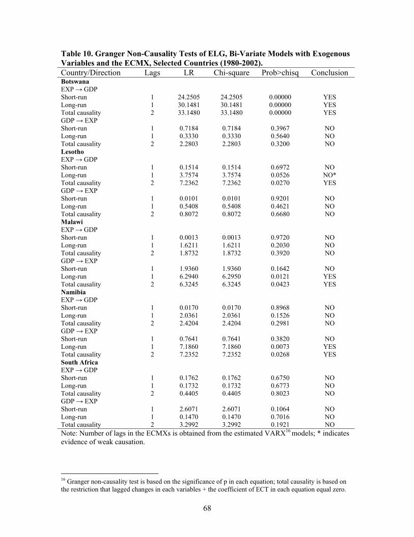
68
Table 10. Granger Non-Causality Tests of ELG, Bi-Variate Models with Exogenous Variables and the ECMX, Selected Countries (1980-2002). Country/Direction Lags LR Chi-square Prob>chisq Conclusion Botswana EXP → GDP Short-run 1 24.2505 24.2505 0.00000 YES Long-run 1 30.1481 30.1481 0.00000 YES Total causality 2 33.1480 33.1480 0.00000 YES GDP → EXP Short-run 1 0.7184 0.7184 0.3967 NO Long-run 1 0.3330 0.3330 0.5640 NO Total causality 2 2.2803 2.2803 0.3200 NO Lesotho EXP → GDP Short-run 1 0.1514 0.1514 0.6972 NO Long-run 1 3.7574 3.7574 0.0526 NO* Total causality 2 7.2362 7.2362 0.0270 YES GDP → EXP Short-run 1 0.0101 0.0101 0.9201 NO Long-run 1 0.5408 0.5408 0.4621 NO Total causality 2 0.8072 0.8072 0.6680 NO Malawi EXP → GDP Short-run 1 0.0013 0.0013 0.9720 NO Long-run 1 1.6211 1.6211 0.2030 NO Total causality 2 1.8732 1.8732 0.3920 NO GDP → EXP Short-run 1 1.9360 1.9360 0.1642 NO Long-run 1 6.2940 6.2950 0.0121 YES Total causality 2 6.3245 6.3245 0.0423 YES Namibia EXP → GDP Short-run 1 0.0170 0.0170 0.8968 NO Long-run 1 2.0361 2.0361 0.1526 NO Total causality 2 2.4204 2.4204 0.2981 NO GDP → EXP Short-run 1 0.7641 0.7641 0.3820 NO Long-run 1 7.1860 7.1860 0.0073 YES Total causality 2 7.2352 7.2352 0.0268 YES South Africa EXP → GDP Short-run 1 0.1762 0.1762 0.6750 NO Long-run 1 0.1732 0.1732 0.6773 NO Total causality 2 0.4405 0.4405 0.8023 NO GDP → EXP Short-run 1 2.6071 2.6071 0.1064 NO Long-run 1 0.1470 0.1470 0.7016 NO Total causality 2 3.2992 3.2992 0.1921 NO Note: Number of lags in the ECMXs is obtained from the estimated VARX16 models; * indicates evidence of weak causation.
16 Granger non-causality test is based on the significance of p in each equation; total causality is based on the restriction that lagged changes in each variables + the coefficient of ECT in each equation equal zero.

69
4.3. Comparative Analysis
4.3.1. Analysis of the ELG Hypothesis in Southern Africa
In the ELG study for Southern Africa, the direction of causation varies from
country to countries due to each country’s characteristics (political and/or economical).
Two types of bi-variate models (common VAR and VARX models) were estimated to
test for the ELG hypothesis in Southern Africa. The results of both types of bi-variate
models show similar conclusions for Mozambique, South Africa, Zambia, and Zimbabwe
(ELG and GDP-led export hypotheses are not valid).
In both types of bi-variate models, the results also show that only the GDP-led
export hypothesis is valid in Malawi and Namibia. Meanwhile, positive and significant
correlation is found between GDP and exports in Malawi, Mozambique, Namibia, South
Africa, and Zimbabwe. Only Mozambique and Zambia report strong correlation between
exports and gross fixed capital formation. Negative correlation between exports and gross
fixed capital formation is found in Malawi. Looking at the ratio of exports to GDP and of
exports and gross fixed capital formation in these countries, it is found that, there is not
significant effect between GDP and exports in most of these countries. For example,
since the 1980s, the ratio of exports to GDP remains almost the same in Malawi,
Namibia, South Africa, Zambia, and Zimbabwe (Appendix A, Figures 35, 37, 38, 40, and
41), while in early 2000, it only showed some increase in Mozambique (Appendix A,
Figure 36).
In the meantime, because of the importance of domestic and foreign investments
in all six countries, it is found that gross fixed capital formation contributes to the
increase in exports in most of these countries. For instance, the ratio of exports to gross
fixed capital formation show that, since the 1980s, this has increased in Malawi, South
70
Africa, and Zimbabwe; it has only decreased in Mozambique and it has remained almost
the same in Zambia (but it increased in early 2000). The rejection of the ELG in all of the
above countries is not that surprising considering each country’s economic performance
over the past years.
Most of these countries have relatively young economies, meaning that their
recent economic growth can be explained by looking at each country’s economic
performance for the past 10 to 20 years. For instance, the latest trade policy reviews of
some of these countries were conducted in 1998 (Namibia and South Africa) and the
most recent trade policy reviews were conducted in early 2000 (Mozambique, Namibia,
South Africa and Zambia). A summary of the trade policy reviews for all Southern
African countries are presented in Table 11 (World Trade Organization-WTO, 2006).
The table includes all countries’ trade liberalization objectives, some trade arrangements,
commitments to trade liberalization, and the principal export commodities (in most recent
years) of each country’s. Over the past years, Malawi, Mozambique, Namibia, South
Africa, Zambia, and Zimbabwe have engaged in economic and trade reforms to promote
economic growth, reduce poverty and unemployment. Most of these countries have
created trade policies that include the diversification of export products. In recent years,
most of these countries are found to have similar export commodities including
agricultural products, beverages and tobacco, crude materials, basic manufactures, and
machinery and transport equipments. For instance, all six countries specialize in the
production of export products in which they have comparative advantage (International
Trade Center—ITC, 2006), although they also produce other products. For example, for
the period 1999-2003, all six countries specialized in the production of fresh food.
Malawi, Namibia, South Africa, and Zimbabwe specialized in the production of
71
processed food. Only Malawi specialized in the production of clothing; and Namibia
specialized in the production of miscellaneous manufactured products. Mozambique,
South Africa, Zambia, and Zimbabwe specialized in the production of basic
manufactured products. Specialization in the production of wood products was performed
in Mozambique and South Africa. Namibia, South Africa, and Zimbabwe specialized in
the production of minerals. Around the world, for the period 1999-2003, in the
production and specialization of fresh food, Malawi ranked 15th, Zimbabwe 27th, Namibia
41st, Mozambique ranked 58th, South Africa 104th, and Zambia 118th. In the production
and specialization of processed food around the world, Malawi ranked 35th, Namibia 27th,
Zimbabwe 76th, and South Africa 89th. In the specialization of basic manufactures,
Zambia ranked number 1st, Mozambique ranked 2nd, South Africa ranked 8th, and
Zimbabwe 19th. In the world market, Malawi ranked 45th in the production of clothing.
South Africa ranked 49th and Mozambique 51st in the production and specialization of
wood products. In the production and specialization of miscellaneous products in the
world market, Namibia ranked 6th. In the production of minerals around the world, South
Africa ranked 63rd, Namibia 68th, and Zimbabwe 70th in the period 1999-2003.
Malawi, Mozambique, Namibia, South Africa, Zambia, and Zimbabwe have
relative open market policies with the commitment to trade liberalization and the creation
of attractive environments for domestic and foreign investments. Although the ELG
hypothesis is not valid in all of these countries, all of them are currently participating in
some regional, bilateral, and multilateral trade agreements with other countries that
contribute to promoting trade liberalization. All six countries participate in trade
arrangements such as the Southern African Customs Union (SACU), the Southern
African Development Community (SADC), and Lomé Convention. The SACU was
72
established in 1910 as a trade arrangement to remove restrictions on the movement of
goods and services between members of the group. SACU’s current members are South
Africa, Namibia, Botswana, Lesotho, and Swaziland (Central Bank of Lesotho, 2004).
The SADC trade protocol (1992) ratified in 1998 (by Botswana) was established as a
mean to lower trade barriers among its member states17 with the following objectives:
achieve development and economic growth, reduce poverty, improve the quality of life of
Southern Africans, and support regional integration to help the less fortunate. The Lomé
Convention is a trade development agreement between the EU and the African,
Caribbean, and Pacific (ACP) States with the advantage of giving member countries free
access to European Markets.
For the remaining three Southern African countries (Botswana, Lesotho, and
Swaziland), the results of the ELG hypothesis in both types of bi-variate models show
some differences when moving from common VAR models to VARX models. The
results on bi-variate models with no exogenous variables show that the ELG hypothesis is
valid in two countries (Lesotho and Swaziland). However, incorporating exogenous
variables into the models, the results show that the ELG hypothesis is valid in three
countries (Botswana, Lesotho, and Swaziland). Looking at the results of the VARX
models, it is concluded that, the validity of the ELG hypothesis in Botswana, Lesotho,
and Swaziland implies that, in the past years, increasing exports of goods and services in
those countries has been a significant contributor to each nation’s economic growth.
These results can be linked to the correlation analysis results since strong and positive
correlation is found between GDP and exports and between exports and gross fixed
17 SADC, 14 Members: Angola, Botswana, Democratic Republic of Congo, Lesotho, Madagascar (membership pending), Malawi, Mauritius, Mozambique, Namibia, Seychelles, South Africa, Swaziland, Tanzania, Zambia, and Zimbabwe.
73
capital formation in all three countries. The correlation between exports and gross fixed
capital formation was also looked at because of each country’s effort in attracting
domestic and foreign investments. For all three countries, only Lesotho reports a positive
trend in the exports to GDP ratio, while the ratio of exports to GDP in Botswana and
Swaziland has remained almost steady over the years. The data also shows positive trend
in the exports to gross fixed capital formation ratio in Lesotho and Swaziland, while this
is declining in Botswana (Appendix A, Figures 33, 34, and 39).
Similar to the above countries, Botswana, Lesotho, and Swaziland are also
considered young economies. These countries’ latest trade reviews were conducted in
1998. They have also engaged in recent economic and trade reforms that contribute to
their economic growth and development. Botswana, Lesotho, and Swaziland have also
developed trade policies that promote the diversification of export products. Their
principal export commodities include products such as textiles, agricultural products
(e.g., meat and meat products, food and live animals, beverages and tobacco and sugar),
and minerals (diamonds, copper, and crud materials). Table 12, 13, and 14 summarize
these countries’ trade performance indices for the period 1999-2003 (ITC, 2006),
including each country’s most principal export products (with respective ranking in the
world market). For the period 1999-2003 (ITC, 2006), the most important export
products in Botswana were fresh food (2% of national export), electronic components
and clothing (each 1% of national export), and minerals (96% of national export).
However, the diversification process in the mineral sector was limited to one product
(Table 13) and the nation’s market diversification strategy only added one mineral
market. In Lesotho, in the period 1999-2003, the most important export product was
clothing, representing 99% of the nation’s exports (Table 12). For the period 1999-2003,

74
Lesotho’s product diversification strategy (clothing sector) added seven equivalent
products with one additional clothing market. For the period 1999-2003, the most
important export products in Swaziland’s were fresh food and wood products (each 6%
of national export), processed food (41% of national export), and textiles (2% of national
export). In Swaziland, the average annual change in per capital exports of processed food
was 11% and that of textile declined by 4%. For the period 1999-2003, Swaziland
diversified its process food products by adding three equivalent process food products,
and it added nine additional equivalent process food markets. In the textile sector, with
the product and market diversification strategies, it added four equivalent products and
six equivalent markets (Table 14). For simplicity, this study does not report the trade
preference indices for Malawi, Mozambique, Namibia, South Africa, Zambia, and
Zimbabwe (all can be found at ITC online).
Overall, even with diversified exports, relative to the world market, Botswana,
Lesotho, and Swaziland, have a comparative advantage in producing some export
products such as minerals (Botswana), clothing (Lesotho and Swaziland), processed food,
wood products, and fresh food (Swaziland). For instance, for the period 1999-2003,
Botswana ranked 6th in the production of minerals around the world. In the production
and specialization of cloth, Lesotho ranked 1st and Swaziland ranked 21st. Swaziland
ranked 5th in the production of processed food, 37th in the production of wood products,
and 110th in the production of fresh food (ITC, 2006). It is reported that these three
countries also have relative open market policies with the commitment to trade
liberalization. For instance, currently, Botswana, Lesotho and Swaziland are also active
members of various multilateral, bilateral, and regional trade arrangements including the
SACU and the SADC.
75
In general, the economic environment of each Southern African country included
in this study is found to be relatively different. In the meantime, recent economic
performance and trade policies in many Southern African countries have contributed to
the explanation of the results obtained regarding the validity of the ELG hypothesis in the
region. Below is a summary of each country’s economic performance for the past few
years.
4.3.2. Botswana
Botswana is known as one of the best performing economies in Africa and one of
the most inspiring stories on the continent (EIU, 2005). Botswana has received the
highest credit rating of reflecting sound management of its resources, a commitment to
democracy, and effective anti-corruption policies (OECD, 2005). In 2002/2003,
Botswana was one of the top performing economies in Sub-Saharan Africa with GDP
growth of 6.7%. Its economy is mostly dependent on the mining industry (mostly
diamonds), which contributes to more than 30% of the nation’s GDP, 80% of the nation’s
total exports, and about 50% of government revenues (EIU, 2005). In 2003/2004, GDP
growth was 5.7% coming mostly from strong growth in the non-mining industry (8.5%).
One of the nation’s strategies for economic development is increasing Foreign Direct
Investment (FDI in 2001, 77% went mostly into the mining sector). The nation has a
trade policy of promoting a sustainable and diversified economy beyond minerals and
diamonds. Botswana is committed to trade liberalization, implying that it is looking
beyond its borders to market its products and services. Botswana has an open market
policy and it is currently an active member of various multilateral, bilateral, and regional
trade arrangements including the EU/RSA Free Trade Agreement. Its exports are
concentrated on a few commodities (minerals), which are mostly exported to Europe. The

76
nation’s major trading partners are the EU, South Africa, and Zimbabwe. Since 2002,
Botswana officially became a beneficiary of the Africa Growth and Opportunity Act. The
success of the nation’s economy and the bulk of Foreign Direct Investment that is going
into its mining sector can explain the findings of the validity of the ELG hypothesis in
this country, implying that exports (especially mineral exports) have contributed to the
economic growth in Botswana. This growth could be continued with increasing exports
(mining and non-mining sectors) as long as the nation continues encouraging domestic
and foreign investments in both the mining and non-mining sectors.
4.3.3. Lesotho
Lesotho is a less developed country with almost 80% of its population living in
rural areas (EIU, 2005). Most of its population lives on farming or migrant labor
(primarily to South Africa mining industry). Lesotho’s extraterritorial migrants account
for 30% of its GDP. Its economy is mostly dependent on water and electricity sold to
South Africa, manufacturing earnings from the Southern African Customs Union
(SACU), agriculture, livestock, and laborers employed in South Africa. Despite
unfavorable weather and food shortages in 2003, GDP grew 3.9%, a 1% increase from
2000. One of the driving forces behind the nation’s GDP growth was strong textile
exports to the US under the African Growth and Opportunity Act (AGOA). This Act is
estimated to continue to be Lesotho’s force of economic growth and job creation.
Through the AGOA, Lesotho has become the largest exporter of garments to the US from
Sub-Saharan Africa. The nation’s participation in AGOA has also enabled it to obtain a
good economic position. Lesotho’s trade and investment objective is to place high
priority in developing exports of diversified manufacture industries and markets. The
nation is committed to create an environment conducive to investment in the private

77
sector. It is also committed to participate in bilateral, regional, and multilateral
negotiations with other countries. Thus, the acceptance of the ELG hypothesis in Lesotho
can be linked to the nation’s dependence on its traditional export products (textiles),
implying that increasing Lesotho’s exports (specialty the production of clothing) through
diversified markets could continue to increase the nation’s economic growth.
4.3.4. Malawi
Malawi’s economy is heavily dependent on agriculture with two major export
crops (tobacco and tea). The nation’s economy depends heavily on agricultural exports,
which makes the nation vulnerable to external shocks (declining TOT and drought).
Agriculture represents 38.6% of GDP and accounts for over 80% of the nation’s labor
force and about 80% of total exports (TDS, 2005). To overcome its vulnerability, since
1981, with assistance from the IMF and other donors, the government of Malawi has
undertaken national reform initiatives such as stimulation of the private sector’s activity,
elimination of price controls and industrial licensing, trade liberalization, and foreign
exchange. Real GDP increased from 2.4% in 2003 to 3.9% in 2004. Malawi’s major
exports come from agricultural products (i.e., tobacco, tea, sugar, coffee, peanuts, and
wood products). Some of Malawi’s major markets include Southern African countries
(South Africa, and Zimbabwe), the US, the EU, the UK, Germany, and Japan. The nation
has a bilateral trade agreement with South Africa and Zimbabwe. Some of the limitations
associated with the export sector in Malawi include low access to the world markets,
limited supply capacity of non-traditional exports, and the nation’s overdependence on
traditional export products. Nevertheless, the nation’s has recently focused on export
development efforts such as adding new export products, diversifying the market, and
consolidating the supply of products, especially within small and medium sized
78
enterprises (SMEs). Although the ELG hypothesis is not valid in this country, based on
its comparative advantage, Malawi should continue specializing in the production of
fresh and processed food, and cloth because these export sectors can continue to
contribute to the nation’s economic growth.
4.3.5. Mozambique
Since the end of the war in 1992, Mozambique has become one of the fastest
growing economies in the world with average growth rate of 8.1% in 1993 (OECD,
2005). In 1998, because of its economic reforms, it became the first African country to
receive debt relief under the Heavily Indebted Poor Countries (HIPC) Initiatives. From
1997 to 1999, its GDP growth averaged almost 10%, more than in the period 1993-1999
(6.7%). In 2001, GDP growth was 14.8% (TDS, 2005); GDP growth in 2003 was 7.1%.
Because of large foreign owned mega projects (The Sasol gas Pipeline and Mozal II
expansion of aluminum smelter), Mozambique’s 2004 economic growth reached 7.8%
(OECD, 2005). Growth in 2003 and 2004 was driven by strong performance in the
extractive and manufacturing industries, good harvests for main export crops, and
abundant demand for transport and communication services (OECD, 2005). The
expansion of the nation’s growth will be supported by major foreign ventures (mega
projects), continuing economic reforms, and the revival of agriculture, transportation, and
tourism. Mozambique’s mega project has contributed to changes in the nation’s balance
of trade. This nation is now the third largest exporter of aluminum to the EU (OECD,
2005); its major export markets (as for 2003) are Belgium, South Africa and Spain.

79
Table 11. Trade Policy Reviews for Southern Africa. Country (last reviews)
Trade liberalization and Investment Policy Objectives
Multilateral, Regional, and bilateral Trade Arrangements
Some Trade Commitments Principal Export Commodities
Botswana (1998)
Promote sustainable diversified economy away from minerals and diamonds
Member: SACU (governs tariff’s policy), SADC (Free trade area within a specified period of time), WTO, and The Lomé Convention. Beneficiary: Trade development agreement between the EU and the African, Caribbean, and Pacific (ACP) States: Advantage of free access to European Markets, EU/RSA (Republic of South Africa) Free Trade Agreement, and AGOA. Some trading partners (exports): SACU, Zimbabwe, other Africa, the UK, and the USA.
Trade liberalization by look beyond borders to market products and services
Meat and meat products; diamonds; copper-nickel matte; textiles; vehicles and parts.
Lesotho (1998)
High priority to the development of exports by Diversification in manufacturing industries and markets
Member: SACU, SADC Trade protocol, and the EU-ACP post-Lomé Convention Proposal. Some trading partners (exports): Africa (SACU), the EU, the USA, and Canada.
Establishment of standards and quality assurance legislation, revision of intellectual property rights legislation and formulation of legislation that promotes competition.
Food and live animals; beverages and tobacco; crud materials; Machinery and transport equipment; miscellaneous manufactured articles.
Malawi (2002)
Create an environment conductive to the good performance of the private sector
Member: Lomé Convention, Common Market of Easter and Southern Africa (COMASA), and SADC. Bilateral agreements: South Africa and Zimbabwe. Beneficiary: AGOA, European Union initiatives: Everything But Arms (EBA). Some trading partners (exports): some members of COMASA, SADC; the EU, the UK, Asia, and the USA.
Committed to participate in multilateral trade
Food and live animals (sugar and honey, coffee, tea, cocoa and spiced tea); beverages and tobacco; basic manufactures (clothing and accessories).
Mozambique (2000)
-Create an environment conductive to promote its products in world markets: Europe, America, Asia, intra-Africa trade. -Speed up industrialization process, to make access to foreign markets easier for its products. - Promote multilateral, regional bilateral and preferential trade agreements.
Member: Lomé Convention, SADC, and IOR-ARC Indian Ocean Rims Association For Regional Cooperation TPA with Africa. Some trading partners (exports): SACU, Belgium, Italy, Portugal, Spain, the UK, and USA. Beneficiary: AGOA, GSP.
-Improve market access for products coming from LDCs (low trade barriers in some particular areas such as agricultural products. -Duty- free and quota-free market access for all products coming from LDCs (help LDCs to address issues such as poverty in those countries).
Food, live animals and tobacco; textile; mineral fuel, lubricants, etc.; basic manufactures (aluminum and alloy, unwrought); machinery and transport equipments.

80
Table 11 Cont. Trade liberalization and Investment Policy Objectives Multilateral, Regional, and bilateral
Trade Arrangements Some Trade Commitments Principal Export Commodities
Namibia (1998)
-Promotion and trade liberalization. -Expansion of exports and diversification of markets and products. -Provision of taxed based incentives for manufacturing enterprises and traders. -Assist small and medium sized enterprises -Create an environment that attracts investments: create a multi-facate incentive regime that concentrates on manufacturing and export-oriented industries.
Member: COMASA, Lomé Convention, and WTO. Preferential trade agreement with: Zimbabwe, SADC, and SACU. Beneficiary: AGOA, Some trading partners (exports): Angola, Canada and the USA, some EU members, South Africa, and the UK.
Open economy, Trade cooperation to secure and enhance export markets and promote international economic cooperation
Food and live animals; beverages and tobacco; crude materials; basic manufactures; machinery and transport equipment; miscellaneous manufactured articles.
South Africa (1998)
-Develop a strategy of integrated trade and industrial policy to promote production (manufactured export growth essential for economic and industry growth). -Enhance international competitiveness, (tariff reduction, termination of export subsidies, and development of SMEs.
Member: SACU, and SADC, and WTO. Beneficiary: AGOA Some trading partners (exports): Angola, SACU, SADC, the EU, UK, USA, Asia, and Middle East.
Build a competitive, fast growing economy that leads to sustainable employment and improvement of the standards of living of all its people
Food and live animals; crude materials; mineral fuel, lubricants, etc; chemicals and related products; basic manufactures; machinery and transport equipment; miscellaneous manufactured articles.
Swaziland (1998)
Expand export sector into new markets and diversify product base (traditional exports produces, sugar, wood, pulp, and citrus, mining sector).
Member: SACU (external trade policy governed by the common external tariff, Lomé Convention, SADC, COMASA Beneficiary: Duty free access to the EU, GSP, AGOA. Some trading partners (exports): Angola, members of COMASA, the UK, and the USA.
-Unilateral lowering of tariffs agreed under the Uruguay Round, the SACU, and SADC Trade Protocol.
Sugar; wood pulp; edible concentrates; textiles; refrigerators.
Zambia (2002)
-Maintain an open market economy (liberalized import and export regime). -Encourage diversification of export market and the production of exportable products. -Support and encourage value added exports of goods. -Look for new markets (regional, international), Ensure efficient customs administration and fair trade practices, and reduce poverty through sustainable economic growth.
Member: COMASA, SADC Trade Protocol, and WTO. Signatory: Cotonou Agreement. Beneficiary: AGOA, EU Everything But Arms (EBA). Some trading partners (exports): Some members of COMASA, SADU, the EU, Asia, and the UK.
-Create an environment conductive for international trade. -Be fully involved in multilateral trading system and committed to objectives, principles and rules of multilateral trading system.
Food and live animals; crude materials; basic manufactures; machinery and transport equipment; miscellaneous manufactured articles (clothing and accessories).
Zimbabwe (no report)
Maintain a open market policy. Member: COMASA and SADC, Some trading partners (exports): SACU and some of its members, China, Europe, the UK, and the USA.
Gradual elimination of import licenses; free the control of foreign exchange; reduce tariff structure; and reduce tariff rates.
Agricultural (tobacco, sugar, etc.); minerals; manufactured articles (ferrous alloys, cotton lint, textiles and clothing, machinery and equipment, and chemicals).
Source: World Trade Organization online Trade Policy Reviews (Government reports) and the Europa World Year Book 2005. Frequency of Trade Reviews depends on country’ size. Least-developed countries have the possibility of a longer review period (more than six years). No recent report is provided for Zimbabwe.

81
Since 2003, Mozambique has become a member of AGOA, giving it access to US
markets (apparel).In the meantime, Mozambique is committed to create an environment
where it can promote its products. It is also committed to accelerate its industrialization
process to facilitate the access of foreign markets. Although no causality is found
between GDP and exports, Mozambique should continue improving the market access of
its products and looking to diversify its export products. The future of Mozambique’s
economic growth will depend on the nation’s commitment to continue specializing in the
production of fresh food, manufactured and wood products.
4.3.6. Namibia
Namibia’s economy is mostly dependent on the production of diamonds and
uranium. The nation’s economy is closely linked to that of South Africa, and its currency
(Namibia dollar) is pegged to the Rand (South Africa’s currency). More that 80% of its
imports come from South Africa (EIU, 2005). The nation exports more than 50% of its
output and imports about 60% of all goods. Over the period 1999-2004, GDP growth rate
averaged 3.4%. Due to high commodity prices, in 2003, GDP growth reached 3.7%. A
significant impediment to Namibia’s growth is Southern African political instability.
Meanwhile, because the sectoral mix of the economy is dominated by minerals which
offer an unusually low degree of self sufficiency, the economy is highly vulnerable to
external shocks. Namibia has a diverse package of export commodities including
diamonds and other minerals (largest share), fish products, beef and meat products,
grapes and light manufactures. The nation is committed to an open market economy,
trade cooperation for securing and enhancing its export markets. Its goals are to expand
exports and diversify its export markets and products. As for 2002, most of Namibia’s
exports went to South Africa and the EU (specially the UK). Europe is becoming its

82
leading market for fish and meat. The nation is a member of AGOA which allows it to
export apparel to the US market. It is an active member of various regional trade
arrangements. Based on the results of the rejection of the ELG hypothesis in this country,
it can be concluded that to promote economic growth in Namibia, the diversification
process best fit the nation’s trade liberalization’s and investment objectives. Meanwhile,
with the nation should continue specializing in the production of fresh and processed
food, and manufactured products to promote economic growth, reduce poverty and
unemployment.
4.3.7. South Africa
South Africa is the world’s largest producer of platinum, gold, chromium and
coal. The nation has well established financial, legal, communications, energy, and
transport systems as well as a well established exchange market. However, most of its
population is still impoverished (EIU, 2005). The level of unemployment is high and
doubling as industries concentrate on capital intensive investments to reduce labor costs
(EIU, 2005). Due to the nation’s highest rate of unemployment, in 2003, GDP growth
was only to 2.8%, down from 3.6% in 2002. In 2004, due to the appreciation of the rand,
and low inflation fostered by high domestic demand and low interest rates, GDP grew by
3.8% (OECD, 2005). In 2006 and 2007, strong demand and a favorable external
environment are expected to increase the nation’s GDP growth to 4%. South Africa
remains one of the strongest nations in Southern Africa, despite its slow economic growth
in the past few years. Its largest trading partner is Europe. In 2004, trade with Europe
accounted for 35% of total exports, China accounted for only 2.5%, and Africa only 13%.
The nation’s trade balance in 2004 deteriorated due to slight increases in the demand of
imported goods, although there was also an increase in exports (OECD, 2005). South

83
Africa is the main source of outward Foreign Direct Investment in Africa (OECD, 2005),
while Foreign Direct Investment to the nation is declining. The nation’s bilateral
agreements are mostly between the SACU members, SADC, and the USA. In the
meantime, this study finds no causal effect from exports to GDP in this country. Thus, to
build a competitive environment, reduce unemployment and poverty, South Africa should
continue to promote the diversification of its export markets and encourage domestic and
foreign direct investments. Even accounting with a diversified export market, the nation
should continue specializing in the production of fresh and processed food, manufactured
and wood products, and minerals. All of these export sectors will continue to contribute
to the nation’s economic growth.
4.3.8. Swaziland
Swaziland ranks among the most prosperous countries in Africa. Since 1968, the
nation has adopted economic development and diversification strategies making it a
middle income nation (EIU, 2005). The most important sector of Swaziland’s economy is
the manufacturing sector. Since the 1980s, when international sanctions reduced the
products made in South Africa, Swaziland’s manufacturing sector has gained market
competitiveness (EIU, 2005). Since the 1970s, Swaziland’s economic growth has been
impressive; however, with its introduction to the SACU, its tax base has been decreasing;
thus, decreasing the nation’s tax revenue. In 2002, the nation’s economic growth was
3.6%. The forces behind this growth included the increase in capital spending due to the
completion of infrastructure projects and higher textile production, supported by the
African Growth and Opportunity Act (AGOA). Swaziland is also an active member of
various trade agreements. As of 2003, its major markets were South Africa (major trading
partner), the EU, Mozambique, and the US. The acceptance of the ELG hypothesis in

84
Swaziland can be explained by the nation’s competitiveness in the production of
manufactured goods (mostly processed food) and its diversified export sector. Its export
markets also include soft drink concentrates, sugar, pulp, canned fruits, and cotton yarn.
The nation is committed to expand its export sector by including new markets and
diversifying its export products base. To continue to promote economic growth, the
nation should continue specializing in the production of goods in which it has a
comparative advantage (processed food, clothing, wood products, and fresh food).
4.3.9. Zambia
Zambia’s economy has always been based on the copper mining industry.
However, since the 1970s with the world’s oil price shocks, static economic policies in
the country and the collapse on copper prices in the world market, Zambia’s economy has
not been increasing as expected. The nation moved from a middle income country to a
poor country. Over the last decade, fearing a continuing rising of domestic debt and the
prospect of missing the HIPC completion point at the end of 2003, the government
developed an economic diversification program to use other resources to improve the
nation’s economy as part of its 2004 fiscal consolidation program (EIU, 2005). The
program included promoting agriculture, tourism, gemstone mining and hydropower.
After two decades of declining growth, GDP growth averaged 4.2% over the period
2000/2003 (EIU, 2005). Major forces contributing to this growth were agriculture,
mining activities, and tourism. In 2003, GDP grew to 4.2%, more than in 2002 (3.3%)
due to agricultural production after the negative effect of the 2002 drought (EIU, 2005).
In 2004, GDP grew 5.1%, accounting for good agricultural performance, strong mining
output, and sizeable private investment (OECD, 2005). In Zambia, minerals account for
the highest share of exported products. Its main trading partner is the SACU. The nation

85
is a member of the Common Market for Eastern and Southern Africa (COMESA) free
trade area agreement. It is also a beneficiary of some preferential market initiatives such
as the General System of Preferences (GSP), the EU’ Everything but Arms Initiative, and
AGOA (OECD, 2005). In 2004, its major markets were South Africa, the UK, Tanzania,
Malawi, and Japan. Some Zambia’s trade policy objectives are to maintain an open
market economy, ensure fair trade practices, and encourage the diversification of its
export markets all of which can increase economic growth, reduce poverty and
unemployment. This study, however, found no causal effect between GDP and exports in
this country. Nevertheless, based on the nation’s comparative advantage in the production
of fresh food and basic manufactured products, the export sector, in this country, can
continue to have an effect on the nation’s economic growth. The production of these
products can also contribute to poverty reduction and unemployment in the country.
4.3.10. Zimbabwe
Relative to other countries in Sub-Saharan Africa, Zimbabwe has the large
deposits of minerals and agricultural commodities. In the period 1980-1981, it
experienced strong economic growth, with GDP growth of more than 20%. However,
since the mid-1990s, the economy has been declining for the following reasons: poor
management of the economy and questionable political and economic policies (TDS,
2005). In 2004, the nation’s GDP experienced a contraction of 4.6%. Because of severe
foreign exchange shortage at the beginning of 2005, high operating cost, lack of
investment, and decreases in production, most sectors of the economy are expected to
continue experiencing negative growth. Other factors contributing to the future
deterioration of Zimbabwe’s economic growth include decreases in consumer spending,
high unemployment, and high inflation rate (EIU, 2005). In recent years, with continued

86
decreases in economic growth, the export sector in Zimbabwe has also faced severe
difficulties denoted by a decrease in all of the sectors (EIU, 2005). In 2003, the
agriculture, hunting, fishing and forestry sectors decreased 8%; mining and quarrying
sectors decreased 9.8%, and the manufacturing sector, 12.2%. The nation’s two largest
foreign exchange earners (tobacco and gold) showed a negative performance in 2004 due
to overvalued exchange rates, foreign currency shortages, and limited rail services. As
long the nation’s political crisis remains unresolved, this negative economic growth could
persist. The negative growth of Zimbabwe’s economy can explain the results obtained
regarding the rejection of both the ELG and the GDP-led export hypotheses in this
country. The nation’s political instability has constantly affected the performance its
export sector. Despite Zimbabwe’s political instability, it is also committed to trade
liberalization, and as other Southern African countries, and has most of its products going
to South Africa, the UK, Germany, and the US. However, the future of this country,
especially the export sector, depends on Zimbabwe’s commitment to continue
specializing in the production of fresh and processed food, manufactured and wood
products, and minerals. All of these sectors can contribute to the nation economic growth
and poverty and unemployment reduction.
Overall, most Southern African countries rely on South Africa as major trading
partner because of its relative economic stability in the region and in Sub-Saharan Africa.
Despite its slow economic growth in the last years, South Africa leads in all
macroeconomic indicators (GDP, exports, gross fixed capital formation, and labor).
However, excluding South Africa, positive increases in real GDP and exports are found
in 7 countries (except in Zimbabwe) and positive increases in gross fixed capital
formation are also seen in 6 countries (except in Malawi and Zimbabwe). At a steady
87
rate, labor in all nine countries is trending upward. The composition of exports in most of
Southern African countries is almost the same. Most of these countries have a
comparative advantage in the production of some products relative to the world (ITC,
2004). For instance, Botswana, South Africa, Namibia, and Zimbabwe have the
comparative advantage in the production (product specialization) of minerals. South
Africa, Mozambique, and Swaziland specialize in the production of wood products.
Swaziland, Malawi, Namibia, Zimbabwe, and South Africa specialize in the production
of processed food. Malawi, Zimbabwe, Namibia, South Africa, and Zambia specialize in
the production of fresh food. Only Lesotho and Swaziland specialize in the production of
cloth. All three countries, in which the ELG hypothesis is valid, specialize in the
production of different export products namely minerals (Botswana), clothing (Lesotho
and Swaziland), and processed food (Swaziland).
This study also found that, the common types of VAR models in ELG and trade
literature are the VAR (p) models. Very little has been done on VARX (p, b) models.
Thus, incorporating VARX models in this thesis brought about new information
concerning the validity of the ELG hypothesis in LDCs. In this study, in bi-variate
models without exogenous variables only GDP and exports are considered, while in
VARX models, gross fixed capital formation and labor are treated as exogenous variables
in the GDP and exports equations. Although the results obtained in both types of
econometric models are not that substantial, VARX models provide more chances of
causation between the variables in more countries since they account for the two most
important inputs of production in most part of Southern Africa. With VARX models, the
number of countries reporting one co-integrating relationship between GDP and exports
is higher than in common VAR models. For instance, in common VAR models, it is

88
found that the ELG hypothesis is valid only Lesotho and Swaziland, while in VARX
models it is valid Botswana, Lesotho, and Swaziland. In general, this study found that,
three out of nine Southern African countries (Botswana, Lesotho, and Swaziland) are
more likely to benefit from export expansion policies than the rest of the countries. Thus,
sound export policies in these countries can continue to contribute to economic growth,
poverty reduction, and job creation.
Table 12. Trade Performance Index for Lesotho (1999-2003). Clothing
INDICATORS Value Rank
(117)* General Profile Value of Exports ($ 000) 426,994 15 Trend of Exports (99-03) P.A 36% Share in National Export 99% Share in National Import 1% Average Annual Change in Per Capita Exports 33% 8
Position In Value Of Net Exports ($ 000) 424,089 36 2003 For Per Capita Exports ($/Inhabitant) 234 15 Current Index Share In World Market 0.18% 54 Product Diversification (N° Of Equivalent Products) 7 86 Market Diversification (N° Of Equivalent Markets) 1 111 Source: International Trade Center (2004); ITC calculations based on COMTRADE of UNSD; ()* ranking out of all exporting countries (number).

89
Table 13. Trade Performance Index for Botswana (1999-2003).
Fresh Food Electronic
Components Clothing Minerals
INDICATORS Value Rank
(173)* Value Rank (99)* Value
Rank (117)* Value
Rank (151)*
General Profile Value of Exports ($ 000) 42,345 23,800 14,042 1,980,282 Trend of Exports (99-03) P.A 0% 142 2% 82 2% 98 5% 72 Share in National Export 2% 1% 1% 96% Share in National Import 0% 8% 5% 3% Average Annual Change in Per Capita Exports -2% 121 1% 64 -9% 111 46% 8 Position In Value of Net Exports ($ 000) 41,431 67 3,013 21 2,369 1,973,628 31 2003 For Per Capita Exports ($/Inhabitant) 24.6 110 13.9 61 8.2 80 1152.7 17 Current Index Share in World Market 0.01% 132 0.00% 73 0.01% 93 0.26% 59 Product Diversification (N° of Equivalent Products) 2 157 1 98 4 103 1 135 Market Diversification (N° of Equivalent Markets) 2 155 1 90 3 67 1 143 Source: International Trade Center (2004); ITC calculations based on COMTRADE of UNSD; ()* ranking out of all exporting countries (number).
Table 14. Trade Performance Index for Swaziland (1999-2003). Fresh food Processed Food Wood Products Textiles
INDICATORS Value Rank
(173)* Value Rank
(146)* Value Rank
(125)* Value Rank
(112)* General Profile Value of Exports ($ 000) 30,714 216'685 31,786 8,850 Trend of Exports (99-03) P.A 3% 118 22% 47 12% 69 30% 21 Share in National Export 6% 41% 6% 2% Share in National Import 2% 3% 0% 24% Average Annual Change in Per Capita Exports 5% 66 11% 43 3% 58 -4% 85 Position in Value of Net Exports ($ 000) 27,107 71 210,796 29 31,212 36 -32,989 48 2003 for Per Capita Exports ($/Inhabitant) 27.5 104 194.2 35 28.5 54 7.9 65 Current Index Share in World Market 0.01% 137 0.07% 77 0.01% 88 0.00% 98 Product Diversification (N° of Equivalent Products) 5 100 3 105 1 120 4 96 Market Diversification (N° of Equivalent Markets) 5 113 9 46 3 98 6 59 Source: International Trade Center (2004); ITC calculations are based on COMTRADE of UNSD; ()* ranking out of all exporting countries (number).
90
CHAPTER 5
SUMMARY, CONCLUSIONS, LIMITATIONS, AND FURTHER RESEARCH
5.1. Summary
The main objective of this study was to empirically test the validity of the ELG
hypothesis in nine Southern African countries using annual data for the period 1980-
2002. Time series techniques were used to test for the causal relationship between GDP
and exports in all nine countries. Three time series techniques were used: unit root tests
(ADF and PP tests), a co-integration test (Johansen’s procedure), and Granger-causality
tests (Likelihood ratio tests).
This research contributes to previous analyses of ELG by conducting a
comparative analysis of econometric time series models with and without exogenous
variables. The bi-variate econometric models are labeled VAR (p) and VARX (p, b) to
denote models with and without exogenous variable effects, respectively. The error-
correction models are labeled as ECMs and ECMXs. Gross fixed capital formation and
labor are the two most important inputs in each Southern African country’s production
functions and are specified as exogenous variables in vector autoregressive processes.
This study presented an alternative solution of mixed order of integration not found in
many empirical papers.
The results of the unit roots test indicated that most of the variables are stationary
in first differences—I(1), except in Botswana, where models for I(2) series were adopted
to test for co-integration and causality between real GDP and real exports. In bi-variate
models with no exogenous variables (VAR), Johansen’s co-integration tests showed that
co-integration (long-run relationships) exists between the GDP and exports in three
91
countries (Botswana, Namibia, and South Africa). In bi-variate models with exogenous
variables, Johansen’s co-integration tests showed that co-integration exists between GDP
and exports in five countries (Botswana, Lesotho, Malawi, Namibia, and South Africa).
All three Granger-causality alternative models were found to be applicable to both types
of bi-variate models (stationary variables, integrated but not co-integrated series, and the
ECM). Granger-causality tests were carried out estimating various SUR systems of
equations (levels, first differences, and ECM models). In all three types of Granger-
causality alternative models, in SUR system of equations, the direction of causation
(unidirectional and/or bidirectional causation) between GDP and exports was tested
calculating the LR test. In both types of bi-variate models (ECMs and ECMXs), the
following null hypotheses were tested: (1) exports do not Granger-cause economic
growth in the short run; (2) exports do not Granger-cause economic growth in the long
run; (3) exports do not cause economic growth in either the short run or the long run. The
GDP-led export Granger non-causality test was also conducted.
The results showed that in bi-variate models with no exogenous variables, the
ELG hypothesis is valid in two countries (Lesotho and Swaziland) and the GDP-led
export growth is also valid in two countries (Malawi and Namibia). Incorporating
exogenous variables into the bi-variate models, the ELG hypothesis becomes valid in
three countries (Botswana, Lesotho, and Swaziland) and GDP-led export is valid in two
countries (Malawi and Namibia).
Overall, only three out of nine countries in Southern Africa are more likely to
benefit from export expansion policies and sound export policies (Botswana, Lesotho,
and Swaziland). All three countries have diversified export markets with the comparative

92
advantage in producing minerals (Botswana), textiles (Lesotho and Swaziland), and
processed food (Swaziland).
5.2. Conclusions
The economic and political situations of each Southern African country included
in this study had an impact on the overall results of the validity of the ELG hypothesis in
this part of the world. This hypothesis is supported only in two countries (Lesotho and
Swaziland) when tested on a bi-variate model with no exogenous variables. Including
gross fixed capital formation and labor as exogenous variables in the analysis, the ELG
hypothesis is found to be valid in three countries (Botswana, Lesotho, and Swaziland).
Both types of bi-variate models included in the study (VAR and VARX) of ELG
in Southern Africa provided similar conclusions in Mozambique, Zambia, and Zimbabwe
(no causality between GDP and exports). Both types of bi-variate models also provided
similar conclusions on the validity of the GDP-led export for Malawi and Namibia.
Although substantial differences were not found in the results of ELG in both types of bi-
variate models, it is very important to account for the two major factors of production
(capital and labor) in the production functions of most Southern African countries. The
VARX models increase the chances of obtaining results otherwise not found in the
common VAR models (i.e., increase in the number of countries reporting a co-integrating
relationship between the variables, five versus three in common VAR models). VARX
models also provide more chances in supporting the ELG hypothesis in more countries
than the VAR models. In the VARX models, three countries (Botswana, Lesotho, and
Swaziland), as oppose to two (VAR models), are more likely to benefit from export
expansion policies that the rest of the countries. Therefore, sound export policies in these
counties can contribute to each nation’s economic growth, poverty reduction, and job

93
creation. In general, although most Southern African countries have adopted export-
friendly policies, the long-run impact of such policies is yet to be observed for most
countries.
5.3. Limitations and Further Research
Some of the limitations associated with this study include the nature of the data
and the sample size used for all countries. In the data used, multicollinearity was found
present. For example, in all countries, labor was found to be a linear combination of one
of the other variables if all variables were treated as endogenous. Thus, the effect of
linear dependence on error correction models should be theoretically examined.
As reported in the last section of the results, most Southern African countries are
committed to trade liberalization by developing commercial policies (export-friendly
policies) that facilitate the movement of goods and services. As this continues to take
place and as more data become available, this study should be re-examined to determine
the short-run, the long-run, and/or the total impact of exports on economic growth,
mostly for Malawi, Mozambique, Namibia, South Africa, Zambia, and Zimbabwe.

94
REFERENCES
Abual-Foul, B. 2004. “Testing the Export-led Growth Hypothesis: Evidence from Jordan.” Applied Economics Letters, 11(6): 393–396.
Abdulai, A. and P. Jaquet. 2002. “Exports and Economic Growth: Co-integration and
Causality Evidence for Cote d'Ivoire.” African Development Review, 14(1): 1-17. Al-Yousif, Y.K. 1997. “Exports and Economic Growth; Some Empirical Evidence from
the Arab Gulf countries”. Applied Economics, 29(6): 693-697. Anderson, K. 2004. “Agriculture, Trade Reform and Poverty Reduction: Implications for
Sub-Saharan Africa.” United Nations Conference on Trade and Development, Policy Issues in International Trade and Commodities, Study Series No. 22. New York and Geneva, http://www.unctad.org/en/docs//itcdtab24_en.pdf.
Anwer, M.S. and R.K Sampath. 1997. “Exports and Economic Growth.” Western
Agricultural Economics Association, Selected Papers of the 1997 Annual Meeting, July 13-16, 1997, Reno/Sparks, Nevada, http://agecon.lib.umn.edu/cgi-bin/view.pl.
Afxentiou, P.C. and A. Serletis. 1991. “Exports and GNP Causality in the Industrial
Countries: 1950-1985.” Kyklos, 44(2): 167-79. Appleyard, D.R. and A.J. Field Jr. 2001. “International Economics.” Edited by P. Shensa
and E. Strathmann, NY. Castro–Zuniga, H. 2004. “Export-led Growth in Honduras and the Central American
Region.” Thesis, Louisiana State University. http://etd.lsu.edu/docs/available/etd-12032004-070104.
Central Bank of Lesotho. 2004. “The SACU-US Free Trade Area (FTA) Negotiations in
Lesotho: An Overview, May 2004.” http://www.centralbank.org.ls/Publications/05_04_Economic_Review.htm.
Darrat, A.F. 1986. “Trade and Development: The Asian Experience.” The Cato Journal,
6(2): 695-699.
Dhawan, U. and B. Biswal. 1999. “Re-Examining Export-led Growth Hypothesis: A Multivariate Co-Integration Analysis for India.” Applied Economics, 31(4): 525-530.
The Economists Intelligence Unit (EIU). 2005. “Country Profile,” Louisiana State University, http://www.lib.lsu.edu/apps/onoffcampus.php, and http://www.eiu.com.
The Europa World Year Book. 2005. “International Organizations, Countries: V. 1: 876;
V. 2: 2680, 2801, 3041, 3085, 3925, 4817, 4834, www.europaworld.com.

95
Ekanayake, E.M. 1999. Exports and Economic Growth in Asian Developing Countries: Co-integration and Error-Correction Models.” Journal of Economic Development, 24(2): 43-56.
Enders, W. 1995. “Applied Econometrics Time Series.” (Wiley, New York). Giles, J.A. and C. L.Williams. 2000. “Export-led Growth: A Survey of the Empirical
Literature and Some Non-causality Results Part 1.” Journal of International Trade & Economic Development, 9(3): 261-337.
Granger, C.W.J. 1969. “Investigating Causal Relations by Econometric Models and
Cross-Spectral Methods.” Journal of Econometrica, 37(3): 424-38. Engle, F.E and C.W.J. Granger. 1987. Co-integration and Error Correction:
Representation, Estimation, and Testing. Econometrica, 55(2): 251-276. Enriques, I. and P. Sadorsky. 1996. “Export-led Growth or Growth-Driven Exports? The
Canadian Case.” Canadian Journal of Economics, 29(3): 540-555. Hachicha, N. 2003. “Exports, Export Composition and Growth: A Simultaneous Error-
Correction Model for Tunisia.” International Economic Journal, 17(1): 101-120. Hertel, T. W., P. V. Preckel, J.A.L. Cranfield and M. Ivanic. 2002. “Poverty Impacts of
Multilateral Trade Liberalization.” Center for Global Trade Analysis, Purdue University, IN, Revised March 31, 2002.
Howard, M. 2002. “Causality between Exports, Imports and Income in Trinidad and
Tobago.” International Economic Journal. 16(4): 97-106. International Trade Center (ITC), UNCTAD/WTO. 2006. “Countries.”
http://www.intracen.org/index.htm. Jin, J.C. 1995. “Export-led Growth and the Four Little Dragons.” Journal of International
Trade & Economic Development, 4(2): 203-215. Jin, J.C. and E. S. H. Yu. 1996. “Export-led Growth and the US economy: another Look.”
Applied Economics Letters, 3(5): 341–344. Johansen, S. 1988. “Statistical Analysis of Cointegration Vectors.” Journal of Economics
Dynamics and Control, 12: 231-54. Johansen, S and K. Joseluis. 1990. “Maximum Likelihood Estimation and Inference on
Cointegration--With Applications to the Demand for Money.” Oxford Bulletin of Economics and Statistics, 54(2): 169-21.
Jung, W.S. P.J. Marshall. 1985. “Exports, Growth and Causality in Developing
Countries.” Journal of Development Economics, 18: 1-12.

96
Kónya, L. 2002. “Exports and Growth: Granger-Causality Analysis on OECD Countries
With a Panel Data Test and Bootstrap Critical Values.” School of Applied Economics, Victoria University, http://members.optusnet.com.au/lkonya/Paper02.pdf#search='Exports%20and%20Growth%3A%20GrangerCausality%20Analysis%20on%20OECD%20Countries.
Medina-Smith, E. J. 2001. “Is The Export-led Growth Hypothesis Valid For Developing Countries? A Case Study of Costa Rica.” University of Sussex, United Kingdom and Universidad de Carabobo, Venezuela, United Nations, New York and Geneva, 2001. http://www.unctad.org/en/docs/itcdtab8_en.pdf#search='Is%20The%20ExportLed%20Growth%20Hypothesis%20Valid%20For%20Developing%20Countries%3F%20A%20Case%20Study%20of%20Costa%20Rica.
Njikam, O. 2003. ‘Exports and economic growth in Sub-Saharan Africa: is there a connection?’ University of Yaoundé, Cameroon, http://www.csae.ox.ac.uk/conferences/2004-GPRaHDiA/papers/3f-ousmanou-CSAE2004.pdf#search='Exports%20and%20economic%20growth%20in%20SubSaharan%20Africa%3A%20is%20there%20a%20connection%3F%E2%80%99.
Organization for Economic Co-operation and Development (OECD). 2005. “African
Economic Outlook 2004/2005-What’s New for Africa?” Nigeria, Africa Development Bank Annual Meeting, May 17 2005,
http://www.oecd.org/document/11/0,2340,en_2649_15162846_34808779_1_1_1_1,00.html, http://www.oecd.org/dev/aeo.
Office of the U.S. Global AIDS Coordinator. “Country, Focus Countries.” U.S. Department of State, http://www.state.gov/s/gac/countries.
Ram, R. 1985. “Exports and Economic Growth: Some Additional Evidence.” Economic Development and Cultural Change, 33(2): 415-425.
Shan, J. and F. Sun. 1998. “On the Export-led Growth Hypothesis: the Econometric Evidence from China.” Applied Economics, 30: 1055-1065.
Siddique, M.A.B and E. A. Selvanathan. 1999. “Export Performance and Economic
Growth: Co-Integration and Causality Analysis for Malaysia, 1966-96.” Australia, gunther.smeal.psu.edu/32246.html.
Sentsho, J. 2002. “Export Revenues as Determinants of Economic Growth: Evidence
from Botswana.” The University of Botswana, http://www.essa.org.za/download/2003Conference/SentshoJ_Exports%20Revenue%20&%20Economic%20GrowthF.pdf#search='Export%20Revenues%20as%20Determinants%20of%20Economic%20Growth%3A%20Evidence%20from%20Botswana'.

97
Travel Document Systems (TDS). 2005. “Africa.” http://www.traveldocs.com.
Yang, M. 2001. “Lag Length and Mean Break in Stationary VAR.” The University of New South Wales, http://www.econometricsociety.org/meetings/am01/content/presented/papers/yang.pdf#search='Lag%20Length%20and%20Mean%20Break%20in%20Stationary%20VAR.
Zapata, H.O and A.N. Rambaldi. 1997. “Monte Carlo Evidence on Co-integration and Causation.” Oxford Bulletin of Econometric and Statistics, 59 (2): 285-298.
World Bank. 2005. “World Development Indicators, Poverty.” http://devdata.worldbank.org/wdipdfs/table2_5.pdf.
World Trade Organization (WTO). 2006. “Trade Policy Reviews.”
http://www.wto.org/english/tratop_e/tpr_e/tp_rep_e.htm#bycountry.

98
APPENDICES

99
APPENDIX A
GRAPHICAL REPRESENTATION FOR SELECTED VARIABLES FOR SOUTHERN AFRICA (1980-2002)
FIGURE 1. Botswana's Real GDP (1980-2002)
0
2000
4000
6000
8000
1980
1982
1984
1986
1988
1990
1992
1994
1996
1998
2000
2002
Period
Mill
ion
US
$
FIGURE 2. Botswana's Real Exports of Goods and Services (1980-2002)
0
1000
2000
3000
4000
1980
1982
1984
1986
1988
1990
1992
1994
1996
1998
2000
2002
Period
Mill
ion
US
$
FIGUR 3. Botswana's Real Gross Fixed Capital Formation (1980-2002)
0
1000
2000
3000
4000
1980
1982
1984
1986
1988
1990
1992
1994
1996
1998
2000
2002
Period
Mill
ion
US
$
FIGUR 4. Botswana's Labor Force (1980-2002)
0
0.2
0.4
0.6
0.8
1
1980
1982
1984
1986
1988
1990
1992
1994
1996
1998
2000
2002
Period
Mill
ion
FIGURE 5. Lesotho's Real GDP (1980-2002)
0200400600800
100012001400
1980
1982
1984
1986
1988
1990
1992
1994
1996
1998
2000
2002
Period
Mill
ion
US
$
FIGURE 6. Lesotho's Real Exports of Goods and Services (1980-2002)
0100200300400500600700
1980
1982
1984
1986
1988
1990
1992
1994
1996
1998
2000
2002
Period
Mill
ion
US
$
FIGURE 7. Lesotho's Real Gross Fixed Capital Formation (1980-2002)
0100200300400500600700
1980
1982
1984
1986
1988
1990
1992
1994
1996
1998
2000
2002
Period
Mill
ion
US
$
FIGURE 8. Lesotho's Labor Force (1980-2002)
00.10.20.30.40.50.60.70.8
1980
1982
1984
1986
1988
1990
1992
1994
1996
1998
2000
2002
Period
Mill
ion

100
FIGURE 9. Malawi's Real GDP(1980-2002)
0
500
1000
1500
2000
1980
1982
1984
1986
1988
1990
1992
1994
1996
1998
2000
2002
Period
Mill
ion
US
$
FIGURE 10. Malawi's Real Exports of Goods and Services (1980-2002)
0100200300400500600700
1980
1982
1984
1986
1988
1990
1992
1994
1996
1998
2000
2002
Period
Mill
ion
US
$
FIGURE 11. Malawi's Real Gross Fixed Capital Formation (1980-2002)
0100200300400500600700800
1980
1982
1984
1986
1988
1990
1992
1994
1996
1998
2000
2002
Period
Mill
ion
US
$
FIGURE 12. Malawi's Labor Force (1980-2002)
01
234
56
1980
1982
1984
1986
1988
1990
1992
1994
1996
1998
2000
2002
PeriodM
illio
n
FIGURE 13. Mozambique's Real GDP (1980-2002)
0
1000
2000
3000
4000
5000
1980
1982
1984
1986
1988
1990
1992
1994
1996
1998
2000
2002
Period
Mill
ion
US
$
FIGURE 14. Mozambique's Real Exports of Goods of Services (1980-2002)
0200400600800
100012001400
1980
1982
1984
1986
1988
1990
1992
1994
1996
1998
2000
2002
Period
Mill
ion
US
$
FIGURE 15. Mozambique's Real Gross Fixed Capital Formation (1980-2002)
0
500
1000
1500
2000
1980
1982
1984
1986
1988
1990
1992
1994
1996
1998
2000
2002
Period
Mill
ion
US
$
FIGURE 16. Mozambique's Labor Force (1980-2002)
0
24
6
810
12
1980
1982
1984
1986
1988
1990
1992
1994
1996
1998
2000
2002
Period
Mill
ion
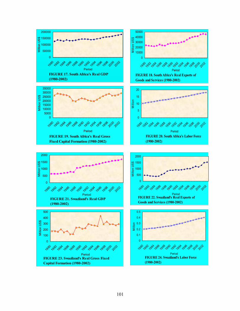
101
FIGURE 17. South Africa's Real GDP (1980-2002)
0
50000
100000
150000
200000
1980
1982
1984
1986
1988
1990
1992
1994
1996
1998
2000
2002
Period
Mill
ion
US
$
FIGURE 18. South Africa's Real Exports of Goods and Services (1980-2002)
0
1000020000
3000040000
50000
1980
1982
1984
1986
1988
1990
1992
1994
1996
1998
2000
2002
Period
Mill
ion
US
$
FIGURE 19. South Africa's Real Gross Fixed Capital Formation (1980-2002)
05000
100001500020000250003000035000
1980
1982
1984
1986
1988
1990
1992
1994
1996
1998
2000
2002
Period
Mill
ion
US
$
FIGURE 20. South Africa's Labor Force (1980-2002)
0
5
10
15
20
1980
1982
1984
1986
1988
1990
1992
1994
1996
1998
2000
2002
PeriodM
illio
n
FIGURE 21. Swaziland's Real GDP (1980-2002)
0
500
1000
1500
2000
1980
1982
1984
1986
1988
1990
1992
1994
1996
1998
2000
2002
Period
Mill
ion
US
$
FIGURE 22. Swaziland's Real Exports of Goods and Services (1980-2002)
0
500
1000
1500
2000
1980
1982
1984
1986
1988
1990
1992
1994
1996
1998
2000
2002
Period
Mill
ion
US
$
FIGURE 23. Swaziland's Real Gross Fixed Capital Formation (1980-2002)
0
100
200
300
400
500
1980
1982
1984
1986
1988
1990
1992
1994
1996
1998
2000
2002
Period
Mill
ion
US
$
FIGURE 24. Swaziland's Labor Force(1980-2002)
0
0.1
0.2
0.3
0.4
0.5
1980
1982
1984
1986
1988
1990
1992
1994
1996
1998
2000
2002
Period
Mill
ion

102
FIGURE 25. Zambia's Real GDP(1980-2002)
01000
20003000
40005000
1980
1982
1984
1986
1988
1990
1992
1994
1996
1998
2000
2002
Period
Mill
ion
US
$
FIGURE 26. Zambia's Real Exports of Goods and Services (1980-2002)
0
500
1000
1500
2000
2500
1980
1982
1984
1986
1988
1990
1992
1994
1996
1998
2000
2002
Period
Mill
ion
US
$FIGURE 27. Zambia's Real Gross Fixed Capital Formation (1980-2002)
0
200
400
600
800
1000
1980
1982
1984
1986
1988
1990
1992
1994
1996
1998
2000
2002
Period
Mill
ion
US
$
FIGURE 28. Zambia's Labor Force(1980-2002)
0
1
2
3
4
5
1980
1982
1984
1986
1988
1990
1992
1994
1996
1998
2000
2002
PeriodM
illio
n
FIGURE 29. Zimbabwe's Real GDP(1980-2002)
0
2000
4000
6000
8000
10000
1980
1982
1984
1986
1988
1990
1992
1994
1996
1998
2000
2002
Period
Mill
ion
US
$
FIGURE 30. Zimbabwe's Real Exports of Goods and Services (1980-2002)
0
1000
2000
3000
4000
1980
1982
1984
1986
1988
1990
1992
1994
1996
1998
2000
2002
Period
Mill
ion
US
$
FIGURE 31. Zimbabwe's Real Gross Fixed Capital Formation (1980-2002)
0
500
1000
1500
2000
1980
1982
1984
1986
1988
1990
1992
1994
1996
1998
2000
2002
Period
Mill
ion
US
$
FIGURE 32. Zimbabwe's Labor Force (1980-2002)
01234567
1980
1982
1984
1986
1988
1990
1992
1994
1996
1998
2000
2002
Period
Mill
ion

103
FIGURE 33. Botswana's Exports-GDP and Export-Gross Fixed Capital Formation Ratios
00.5
11.5
22.5
33.5
1980
1982
1984
1986
1988
1990
1992
1994
1996
1998
2000
2002
Period
Rat
ioEXP/GDPEXP/GFCF
FIGURE 34. Lesotho's Exports-GDP and Export-Gross Fixed Capital Formation Ratios
00.20.40.60.8
11.21.4
19801982
19841986
198819
901992
199419
9619
982000
2002
Period
Rat
io
EXP/GDP
EXP/GFCF
FIGURE 35. Malawi's Exports-GDP and Export-Gross Fixed Capital Formation Ratios
0
0.5
1
1.5
2
2.5
3
1980
1982
1984
1986
1988
1990
1992
1994
1996
1998
2000
2002
Period
Rat
io
EXP/GDPEXP/GFCF
FIGURE 36. Mozambique's Exports-GDP and Exports-Gross Fixed Capital Formation Ratios
00.20.40.60.8
11.21.4
1980
1982
1984
1986
1988
1990
1992
1994
1996
1998
2000
2002
PeriodR
atio
EXP/GDPEXP/GFCF
FIGURE 37. Namibia's Exports-GDP and Exports-Gross Fixed Capital Formation Ratios
00.5
11.5
22.5
33.5
44.5
1980
1982
1984
1986
1988
1990
1992
1994
1996
1998
2000
2002
Period
Rat
io
EXP/GDPEXP/GFCF
FIGURE 38. South Africa's Exports-GDP and Exports-Gross Fixed Capital Formation Ratios
0
0.3
0.6
0.9
1.2
1.5
1.8
1980
1982
1984
1986
1988
1990
1992
1994
1996
1998
2000
2002
Period
Rat
io
EXP/GDPEXP/GFCF
FIGURE 39. Swaziland's Exports-GDP and Exports-Gross Fixed Capital Formation Ratios
0
1
2
3
4
5
6
1980
1982
1984
1986
1988
1990
1992
1994
1996
1998
2000
2002
Period
Rat
io
EXP/GDPEXP/GFCF
FIGURE 40. Zambia's Exports-GDP and Exports-Gross Fixed Capital Formation Ratios
0
1
2
3
4
5
6
1980
1982
1984
1986
1988
1990
1992
1994
1996
1998
2000
2002
Period
Rat
io
EXP/GDPEXP/GFCF

104
FIGURE 41. Zimbabwe's Exports-GDP and Exports-Gross Fixed Capital Formation Ratios
00.5
11.5
22.5
33.5
44.5
5
1980
1982
1984
1986
1988
1990
1992
1994
1996
1998
2000
2002
Period
Rat
io
EXP/GDPEXP/GFCF

105
APPENDIX B PEARSON’S CORRELATION COEFFICIENTS FOR SELECTED VARIABLES,
SOUTHERN AFRICA (1980-2002)
Table 1. Correlation Analysis For GDP, Exports, Gross Fixed Capital Formation and Labor, For Southern Africa (Log-Log Series), (1980-2002). GDP-EXP GDP-GFCF GDP-LAB EXP-GFCF EXP-LAB Botswana 0.96444
(<.0001) 0.95219 (<.0001)
0.98875 (<.0001)
0.88121 (<.0001)
0.94050 (<.0001)
Lesotho 0.94490 (<.0001)
0.94038 (<.0001)
0.98044 (<.0001)
0.83625 (<.0001)
0.93631 (<.0001)
Malawi 0.92498 (<.0001)
-0.80085 (<.0001)
0.96022 (<.0001)
-0.74625 (<.0001)
0.87952 (<.0001)
Mozambique 0.95391 (<.0001)
0.96449 (<.0001)
0.89601 (<.0001)
0.88959 (<.0001)
0.82516 (<.0001)
Namibia 0.90883 (<.0001)
0.82804 (<.0001)
0.97821 (<.0001)
0.72822 (<.0001)
0.89329 (<.0001)
South Africa 0.96347 (<.0001)
0.36017 (0.0914)
0.93148 (<.0001)
0.30035 (0.1638)
0.95788 (<.0001)
Swaziland 0.97532 (<.0001)
0.82742 (<.0001)
0.95671 (<.0001)
0.77730 (<.0001)
0.93407 (<.0001)
Zambia 0.29992 (0.1644)
0.19475 (0.3732)
0.81144 (<.0001)
0.75682 (<.0001)
0.14875 (0.4982)
Zimbabwe 0.93869 (<.0001)
0.60337 (0.0023)
0.93937 (<.0001))
0.42858 (0.0413)
0.94201 (<.0001)
Note : Values in parentheses are the probabilities the Prob > |r| under H_0: Rho=0, where r is the correlation coefficient.

106
APPENDIX C
AUGMENTED DICKEY-FULLER AND PHILIPS-PERRON UNIT ROOT TESTS, SELECTED VARIABLES (1980-2002)
Table 2. Augmented Dickey-Fuller and Phillips-Perron Unit Root Tests on GDP, Exports, Gross Fixed Capital Formation and Labor for Botswana (1980-2002).
Unit Root Tests In Levels Unit Root Tests In First Differences ADF-test PP-test ADF-test PP-test
Equation Series/ Opt. Lag (ADF)
Null Hypothesis (Unit Root)
T-Stat Decision I(d)
T-Stat Decision I(d)
Opt. Lag (ADF)
T-Stat Decision I(d)
T-Stat Decision I(d)
lnGDP Constant 1 γ =0 -2.1198 I(1) -2.84 I(0) 4 -0.8249 I(2) -1.8778 I(2) Constant, trend
1 γ =0 γ =a2=0
-1.897 3.4216
I(1) I(1)
-1.09 4.054
I(1) I(1)
4 -1.8732 1.7944
(2) (2)
-2.5960 3.5165
I(2) I(2)
lnEXP Constant, no trend
0 γ =0 -2.9135 I(0) -2.87 I(0) 2 -2.2992
(2) -3.1521 I(1)
Constant, trend
0 γ =0 γ =a2=0
-1.9055 4.6171
I(1) I(1)
-1.91 4.537
I(1) I(1)
2 -2.0741 2.6843
(2) (2)
-3.9324 7.9930
I(1) I(1)
lnGFCF Constant, no trend
0 γ =0 0.5860 I(1) 0.427 I(1) 0 -1.7243 (2) -1.8513 I(2)
Constant, trend
0 γ =0 γ =a2=0
-1.6209 2.1018
I(1) I(1)
-1.84 2.397
I(1) I(1)
0 -1.7008 2.1649
(2) (2)
-1.8999 2.5032
I(2) I(2)
lnLAB Constant, no trend
1 γ =0 -1.5804 I(1) -4.55 I(0) 1 1.0454 (2) 2.8410 I(1)
Constant, trend
1 γ =0 γ =a2=0
-0.2089 1.1935
I(1) I(1)
7.077 100.1
I(0) I(0)
1 -0.2245 1.9099
(2) (2)
0.4290 5.5814
I(2) I(1)
Note: ADF and PP test 10% critical values: Null hypotheses (levels and in first diff): constant and no trend (-2.57); constant and a trend, for γ =0 (-3.13), for γ =a2=0 (5.34).
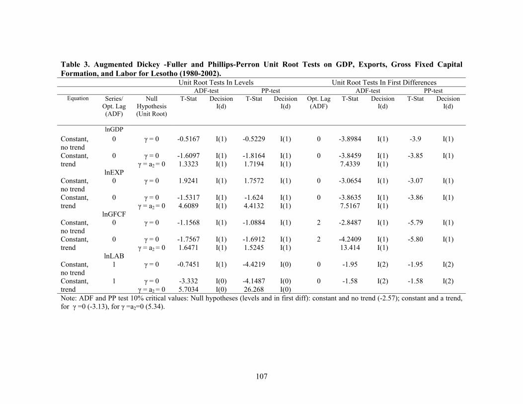
107
Table 3. Augmented Dickey -Fuller and Phillips-Perron Unit Root Tests on GDP, Exports, Gross Fixed Capital Formation, and Labor for Lesotho (1980-2002).
Unit Root Tests In Levels Unit Root Tests In First Differences ADF-test PP-test ADF-test PP-test
Equation Series/ Opt. Lag (ADF)
Null Hypothesis (Unit Root)
T-Stat Decision I(d)
T-Stat Decision I(d)
Opt. Lag (ADF)
T-Stat Decision I(d)
T-Stat Decision I(d)
lnGDP Constant, no trend
0 γ = 0 -0.5167 I(1) -0.5229 I(1) 0 -3.8984 I(1) -3.9 I(1)
Constant, trend
0 γ = 0 γ = a2 = 0
-1.6097 1.3323
I(1) I(1)
-1.8164 1.7194
I(1) I(1)
0 -3.8459 7.4339
I(1) I(1)
-3.85 I(1)
lnEXP Constant, no trend
0 γ = 0 1.9241 I(1) 1.7572 I(1) 0 -3.0654 I(1) -3.07 I(1)
Constant, trend
0 γ = 0 γ = a2 = 0
-1.5317 4.6089
I(1) I(1)
-1.624 4.4132
I(1) I(1)
0 -3.8635 7.5167
I(1) I(1)
-3.86 I(1)
lnGFCF Constant, no trend
0 γ = 0 -1.1568 I(1) -1.0884 I(1) 2 -2.8487 I(1)
-5.79 I(1)
Constant, trend
0 γ = 0 γ = a2 = 0
-1.7567 1.6471
I(1) I(1)
-1.6912 1.5245
I(1) I(1)
2 -4.2409 13.414
I(1) I(1)
-5.80 I(1)
lnLAB Constant, no trend
1 γ = 0 -0.7451 I(1) -4.4219 I(0) 0 -1.95 I(2) -1.95 I(2)
Constant, trend
1 γ = 0 γ = a2 = 0
-3.332 5.7034
I(0) I(0)
-4.1487 26.268
I(0) I(0)
0 -1.58 I(2) -1.58 I(2)
Note: ADF and PP test 10% critical values: Null hypotheses (levels and in first diff): constant and no trend (-2.57); constant and a trend, for γ =0 (-3.13), for γ =a2=0 (5.34).

108
Table 4. Augmented Dickey-Fuller and Phillips-Perron Unit Root Tests on GDP, Exports, Gross Fixed Capital Formation, and Labor for Malawi (1980-2002).
Unit Root Tests In Levels Unit Root Tests In First Differences ADF-test PP-test ADF-test PP-test
Equation Series/ Opt. Lag (ADF)
Null Hypothesis (Unit Root)
T-Stat Decision I(d)
T-Stat Decision I(d)
Opt. Lag (ADF)
T-Stat Decision I(d)
T-Stat Decision I(d)
LnGDP Constant, no trend
0 γ = 0 -0.5204 I(1) -0.3221 I(1) 1 -3.4240 I(1) -7.2895 I(1)
Constant, trend
0 γ = 0 γ = a2 =0
-3.9979 8.0161
I(0) I(0)
-4.0027 8.0476
I(0) I(0)
1 -3.2934 5.8317
I(1) I(1)
-7.1003 25.371
I(1) I(1)
LnEXP Constant, no trend
0 γ = 0 -1.008 I(1) -0.999 I(1) 1 -4.5375 I(1) -5.1695 I(1)
Constant, trend
0 γ = 0 γ = a2 = 0
-3.9499 7.9584
I(1) I(0)
-3.967 8.0766
I(0) I(0)
1 -4.4035 10.100
I(1) I(1)
-4.9479 12.545
I(1) I(1)
LnGFCF
Constant, no trend
4 γ = 0 -0.3176 I(1) -1.4279 I(1) 0 -4.4748 I(1) -4.4701 I(1)
Constant, trend
4 γ = 0 γ = a2 = 0
-1.5124 1.2594
I(1) I(1)
-2.1778 2.4357
I(1) I(1)
0 -4.3490 9.8791
I(1) I(1)
-4.3484 9.8778
I(1) I(1)
LnLAB Constant, no trend
1 γ = 0 -1.337 I(1) -3.0757 I(0) 0 -1.4635 I(2) -1.4976 I(2)
Constant, trend
1 γ = 0 γ = a2 = 0
-2.58 3.8639
I(1) I(1)
-1.5651 5.4806
I(1) I(1)
0 -1.6953 1.4681
I(2) I(2)
-1.7850 1.6436
I(2) I(2)
Note: ADF and PP test 10% critical values: Null hypotheses (levels and in first diff): constant and no trend (-2.57); constant and a trend, for γ =0 (-3.13), for γ =a2=0 (5.34).

109
Table 5. Augmented Dickey-Fuller and Phillips-Perron Unit Root Tests on GDP, Exports, Gross Fixed Capital Formation, and Labor for Mozambique (1980-2002).
Unit Root Tests In Levels Unit Root Tests In First Differences ADF-test PP-test ADF-test PP-test
Equation Series/ Opt. Lag (ADF)
Null Hypothesis (Unit Root)
T-Stat Decision I(d)
T-Stat Decision I(d)
Opt. Lag (ADF)
T-Stat Decision I(d)
T-Stat Decision I(d)
lnGDP Constant, no trend
0 γ = 0 1.4346 I(1) 1.0928 I(1) 0 -2.7676 I(1) -2.7684 I(1)
Constant, trend
0 γ = 0 γ = a2 = 0
-1.6724 6.1470
I(1) I(0)
-1.6807 5.8839
I(1) I(0)
0 -3.9364 7.8020
I(1) I(1)
-3.9510 7.8970
I(1) I(1)
lnEXP Constant, no trend
1 γ = 0 0.2211 I(1) 1.0511 I(1) 0 -2.5786 I(1) -2.5322 I(2)
Constant, trend
1 γ = 0 γ = a2 = 0
-2.1783 5.6318
I(1) I(0)
-2.0753 13.371
I(1) I(0)
0 -3.6511 6.7916
I(1) I(1)
-3.6599 6.8328
I(1) I(1)
lnGFCF Constant, no trend
0 γ = 0 1.7612 I(1) 1.9613 I(1) 3 -0.6868 I(2) -3.7623 I(1)
Constant, trend
0 γ = 0 γ = a2 = 0
-0.9035 3.4034
I(1) I(1)
-0.8069 3.6075
I(1) I(1)
3 -1.6188 1.3918
I(2) I(2)
-4.8948 12.062
I(1) I(1)
lnLAB Constant, no trend
1 γ = 0 1.1845 I(1) 1.3308 I(1) 0 -1.2109 I(2) -1.3552 I(2)
Constant, trend
1 γ = 0 γ = a2 = 0
-2.7954 6.2193
I(1) I(0)
-0.3430 1.0298
I(1) I(1)
0 -1.8658 2.5011
I(2) I(2)
-1.9025 2.4811
I(2) I(2)
Note: ADF and PP test 10% critical values: Null hypotheses (levels and in first diff): constant and no trend (-2.57); constant and a trend, for γ =0 (-3.13), for γ =a2=0 (5.34).

110
Table 6. Augmented Dickey-Fuller and Phillips-Perron Unit Root Tests on GDP, Exports, Gross Fixed Capital Formation, and Labor for Namibia (1980-2002).
Unit Root Tests In Levels Unit Root Tests In First Differences ADF-test PP-test ADF-test PP-test
Equation Series/ Opt. Lag (ADF)
Null Hypothesis (Unit Root)
T-Stat Decision I(d)
T-Stat Decision I(d)
Opt. Lag (ADF)
T-Stat Decision I(d)
T-Stat Decision I(d)
lnGDP Constant, no trend
0 γ = 0 1.3008 I(1) 1.2365 I(1) 2 -2.4347 I(1) -3.6938 I(1)
Constant, trend
0 γ = 0 γ = a2 = 0
-2.7125 6.2610
I(1) I(0)
-2.7539 6.6425
I(1) I(0)
2 -2.1286 2.9814
I(2) I(2)
-4.1367 8.5915
I(1) I(1)
lnEXP Constant, no trend
0 γ = 0 -0.8062 I(1) -0.8426 I(1) 0 -4.4275 I(1) -4.4278 I(1)
Constant, trend
0 γ = 0 γ = a2 = 0
-3.1575 5.1941
I(0) I(1)
-3.2109 5.3964
I(0) I(0)
0 -4.3037 9.2854
I(1) I(1)
-4.3019 9.2667
I(1) I(1)
lnGFCF Constant, no trend
0 γ = 0 -0.6032 I(1) -0.5886 I(1) 2 -2.4326 I(2) -4.6829 I(1)
Constant, trend
0 γ = 0 γ = a2 = 0
-2.9578 6.6044
I(1) I(0)
-3.2512 8.8171
I(0) I(0)
2 -1.5938 2.7801
I(2) I(2)
-5.4062 14.819
I(1) I(1)
lnLAB Constant, no trend
2 γ = 0 -1.8446 I(1) 0.3690 I(1) 1 -3.4482 I(1) -1.7872 I(2)
Constant, trend
2 γ = 0 γ = a2 = 0
-0.3988 1.6558
I(1) I(1)
-2.0209 2.2696
I(1) I(1)
1 -3.4034 8.4108
I(1) I(1)
-1.4003 3.0359
I(2) I(2)
Note: ADF and PP test 10% critical values: Null hypotheses (levels and in first diff): constant and no trend (-2.57); constant and a trend, for γ =0 (-3.13), for γ =a2=0 (5.34).

111
Table 7. Augmented Dickey-Fuller and Phillips-Perron Unit Root Tests on GDP, Exports, Gross Fixed Capital Formation, and Labor for South Africa (1980-2002).
Unit Root Tests In Levels Unit Root Tests In First Differences ADF-test PP-test ADF-test PP-test
Equation Series/ Opt. Lag (ADF)
Null Hypothesis (Unit Root)
T-Stat Decision I(d)
T-Stat Decision I(d)
Opt. Lag (ADF)
T-Stat Decision I(d)
T-Stat Decision I(d)
lnGDP Constant, no trend
0 γ = 0 0.2596 I(1) 0.3927 I(1) 0 -5.4261 I(1) -5.3622 I(1)
Constant, trend
0 γ = 0 γ = a2 = 0
-1.6109 1.7216
I(1) I(1)
-1.5833 1.6824
I(1) I(1)
0 -6.2245 20.008
I(1) I(1)
-6.2420 20.113
I(1) I(1)
lnEXP Constant, no trend
0 γ = 0 0.7775 I(1) 0.6568 I(1) 2 -3.2863 I(1) -3.7209 I(1)
Constant, trend
0 γ = 0 γ = a2 = 0
-3.1252 6.7590
I(1) I(0)
-3.0818 6.4402
I(1) I(0)
2 -2.7877 5.2695
I(2) I(1)
-3.5343 6.9023
I(1) I(1)
lnGFCF Constant, no trend
0 γ = 0 -1.0789 I(1) -1.3834 I(1) 0 -2.7894 I(1) -2.9473 I(1)
Constant, trend
0 γ = 0 γ = a2 = 0
-1.0883 1.4454
I(1) I(1)
-1.3312 1.5361
I(1) I(1)
0 -3.1688 5.3441
I(1) I(1)
-3.2609 5.6705
I(1) I(1)
lnLAB Constant, no trend
1 γ = 0 -1.6894 I(1) -2.7749 I(0) 1 -1.3203 I(2) -0.4216 I(2)
Constant, trend
1 γ = 0 γ = a2 = 0
-1.3907 2.3637
I(1) I(1)
-1.1289 4.465
I(1) I(1)
1 -2.5921 4.4640
I(2) I(2)
-1.2364 1.7121
I(2) I(2)
Note: ADF and PP test 10% critical values: Null hypotheses (levels and in first diff): constant and no trend (-2.57); constant and a trend, for γ =0 (-3.13), for γ =a2=0 (5.34).

112
Table 8. Augmented Dickey-Fuller and Phillips-Perron Unit Root Tests on GDP, Exports, Gross Fixed Capital Formation, and Labor for Swaziland (1980-2002).
Unit Root Tests In Levels Unit Root Tests In First Differences ADF-test PP-test ADF-test PP-test
Equation Series/ Opt. Lag (ADF)
Null Hypothesis (Unit Root)
T-Stat Decision I(d)
T-Stat Decision I(d)
Opt. Lag (ADF)
T-Stat Decision I(d)
T-Stat Decision I(d)
lnGDP Constant, no trend
0 γ = 0 -1.3425 I(1) -1.2302 I(1) 1 -2.7710 I(1) -5.8298 I(1)
Constant, trend
0 γ = 0 γ = a2 = 0
1.3241 2.4426
I(1) I(1)
6.9828 26.570
I(0) I(0)
1 -2.9256 4.4591
I(2) I(2)
-5.8306 17.045
I(1) I(1)
lnEXP Constant, no trend
0 γ = 0 -1.5918 I(1) -1.4071 I(1) 0 -2.8767 I(1) -2.8491 I(1)
Constant, trend
0 γ = 0 γ = a2 = 0
-0.0532 1.3989
I(1) I(1)
0.2841 1.4440
I(1) I(1)
0 -2.7884 3.9422
I(2) I(2)
-2.7635 3.8585
I(2) I(2)
lnGFCF Constant, no trend
0 γ = 0 -0.9412 I(1) -0.9379 I(1) 3 -2.3633 I(1) -6.7329 I(1)
Constant, trend
0 γ = 0 γ = a2 = 0
0.5424 1.5912
I(1) I(1)
2.6042 4.9824
I(1) I(1)
3 -2.2666 2.7099
I(2) I(2)
-6.5500 21.348
I(1) I(1)
lnLAB Constant, no trend
0 γ = 0 -1.7403 I(1) -1.5635 I(1) 0 -1.0430 I(2) -1.2109 I(2)
Constant, trend
0 γ = 0 γ = a2 = 0
-0.2304 1.4474
I(1) I(1)
2.4378 4.3622
I(1) I(1)
0 -0.2290 0.9950
I(2) I(2)
-0.47297 0.9228
I(2) I(2)
Note: ADF and PP test 10% critical values: Null hypotheses (levels and in first diff): constant and no trend (-2.57); constant and a trend, for γ =0 (-3.13), for γ =a2=0 (5.34).
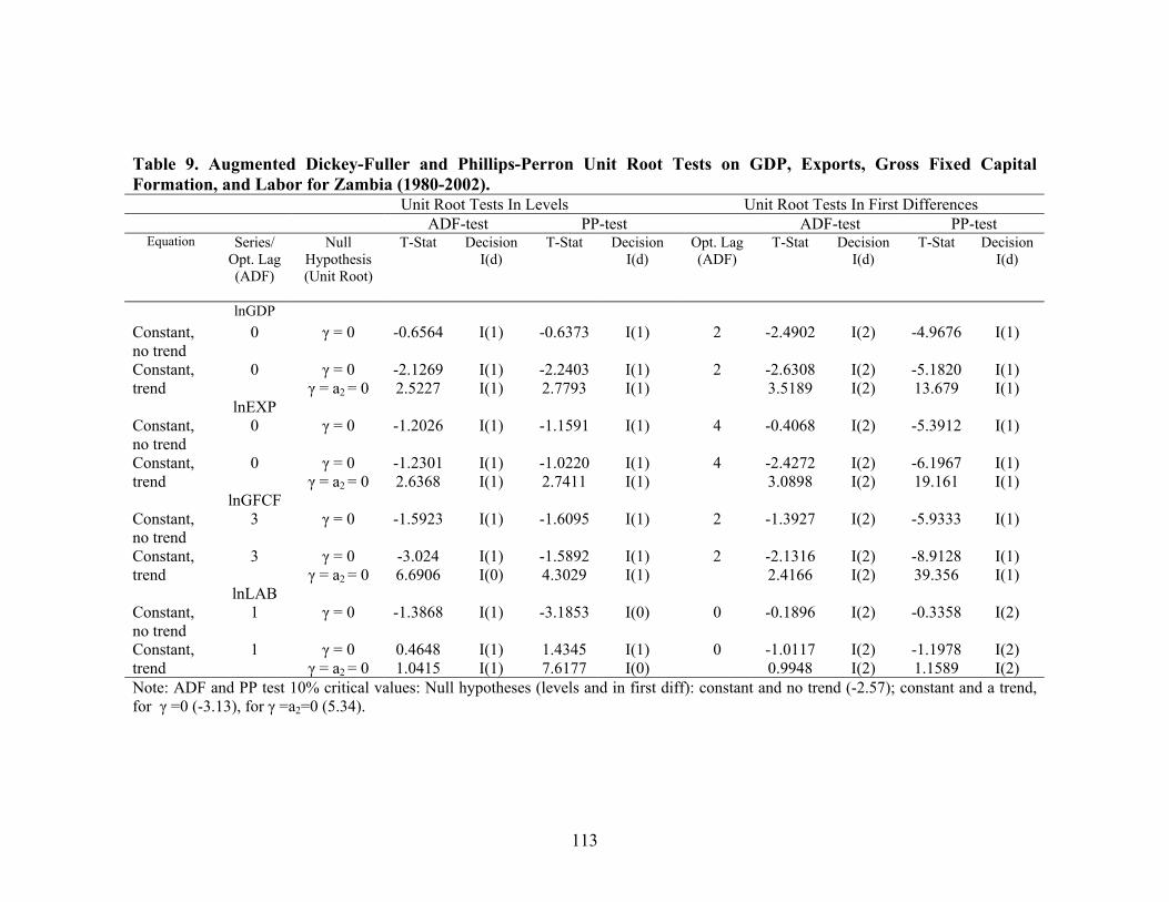
113
Table 9. Augmented Dickey-Fuller and Phillips-Perron Unit Root Tests on GDP, Exports, Gross Fixed Capital Formation, and Labor for Zambia (1980-2002).
Unit Root Tests In Levels Unit Root Tests In First Differences ADF-test PP-test ADF-test PP-test
Equation Series/ Opt. Lag (ADF)
Null Hypothesis (Unit Root)
T-Stat Decision I(d)
T-Stat Decision I(d)
Opt. Lag (ADF)
T-Stat Decision I(d)
T-Stat Decision I(d)
lnGDP Constant, no trend
0 γ = 0 -0.6564 I(1) -0.6373 I(1) 2 -2.4902 I(2) -4.9676 I(1)
Constant, trend
0 γ = 0 γ = a2 = 0
-2.1269 2.5227
I(1) I(1)
-2.2403 2.7793
I(1) I(1)
2 -2.6308 3.5189
I(2) I(2)
-5.1820 13.679
I(1) I(1)
lnEXP Constant, no trend
0 γ = 0 -1.2026 I(1) -1.1591 I(1) 4 -0.4068 I(2) -5.3912 I(1)
Constant, trend
0 γ = 0 γ = a2 = 0
-1.2301 2.6368
I(1) I(1)
-1.0220 2.7411
I(1) I(1)
4 -2.4272 3.0898
I(2) I(2)
-6.1967 19.161
I(1) I(1)
lnGFCF Constant, no trend
3 γ = 0 -1.5923 I(1) -1.6095 I(1) 2 -1.3927 I(2) -5.9333 I(1)
Constant, trend
3 γ = 0 γ = a2 = 0
-3.024 6.6906
I(1) I(0)
-1.5892 4.3029
I(1) I(1)
2 -2.1316 2.4166
I(2) I(2)
-8.9128 39.356
I(1) I(1)
lnLAB Constant, no trend
1 γ = 0 -1.3868 I(1) -3.1853 I(0) 0 -0.1896 I(2) -0.3358 I(2)
Constant, trend
1 γ = 0 γ = a2 = 0
0.4648 1.0415
I(1) I(1)
1.4345 7.6177
I(1) I(0)
0 -1.0117 0.9948
I(2) I(2)
-1.1978 1.1589
I(2) I(2)
Note: ADF and PP test 10% critical values: Null hypotheses (levels and in first diff): constant and no trend (-2.57); constant and a trend, for γ =0 (-3.13), for γ =a2=0 (5.34).

114
Table 10. Augmented Dickey-Fuller and Phillips-Perron Unit Root Tests on GDP, Exports, Gross Fixed Capital Formation, and Labor for Zimbabwe (1980-2002).
Unit Root Tests in Levels Unit Root Tests in First Differences ADF-test PP-test ADF-test PP-test
Equation Series/ Opt. Lag (ADF)
Null Hypothesis (Unit Root)
T-Stat Decision I(d)
T-Stat Decision I(d)
Opt. Lag (ADF)
T-Stat Decision I(d)
T-Stat Decision I(d)
lnGDP Constant, no trend
0 γ = 0 -2.2859 I(1) -2.1923 I(1) 0 -3.4916 I(1) -3.4988 I(1)
Constant, trend
0 γ = 0 γ = a2 = 0
-0.3621 2.5518
I(1) I(1)
-0.6706 2.3393
I(1) I(1)
0 -3.7995 7.2300
I(1) I(1)
-3.8156 7.3208
I(1) I(1)
lnEXP Constant, no trend
0 γ = 0 -0.9891 I(1) -0.9723 I(1) 2 -1.0293 I(2) -3.1823 I(1)
Constant, trend
0 γ = 0 γ = a2 = 0
-0.9712 0.7701
I(1) I(1)
-1.3535 1.1679
I(1) I(1)
2 -0.6706 1.0259
I(2) I(2)
-3.1290 4.9442
I(2) I(2)
lnGFCF Constant, no trend
0 γ = 0 -1.0392 I(1) -1.2200 I(1) 2 -1.4027 I(2) -3.2518 I(1)
Constant, trend
0 γ = 0 γ = a2 = 0
0.1232 2.6648
I(1) I(1)
0.0148 2.4338
I(1) I(1)
2 -2.5032 3.5127
I(2) I(2)
-3.7709 7.1407
I(1) I(1)
lnLAB Constant, no trend
2 γ = 0 -2.5161 I(1) -8.5063 I(0) 0 -0.2609 I(2) -0.3601 I(2)
Constant, trend
2 γ = 0 γ = a2 = 0
-2.2045 4.4542
I(1) I(1)
-1.0214 35.244
I(1) I(0)
0 -1.5193 1.2138
I(2) I(2)
-1.6961 1.5227
I(2) I(2)
Note: ADF and PP test 10% critical values: Null hypotheses (levels and in first diff): constant and no trend (-2.57); constant and a trend, for γ =0 (-3.13), for γ =a2=0 (5.34).
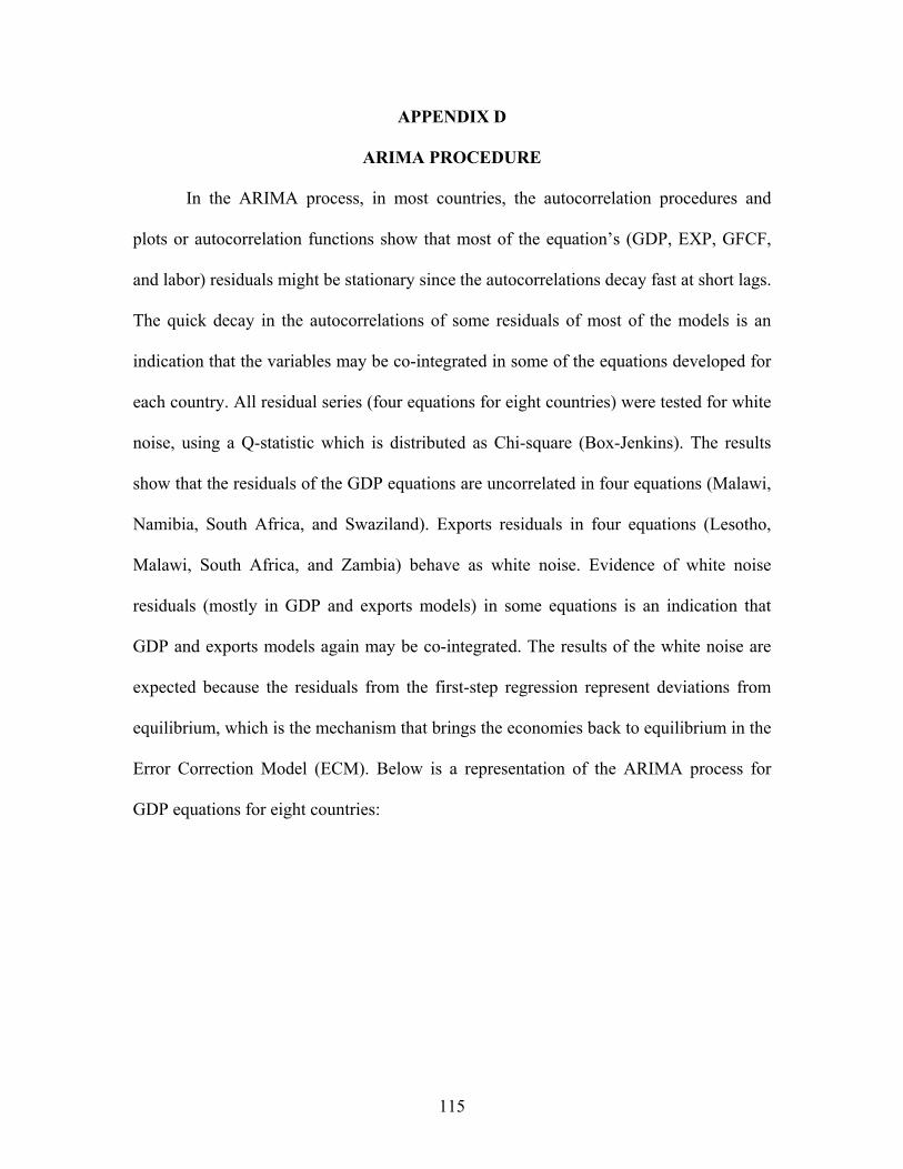
115
APPENDIX D
ARIMA PROCEDURE
In the ARIMA process, in most countries, the autocorrelation procedures and
plots or autocorrelation functions show that most of the equation’s (GDP, EXP, GFCF,
and labor) residuals might be stationary since the autocorrelations decay fast at short lags.
The quick decay in the autocorrelations of some residuals of most of the models is an
indication that the variables may be co-integrated in some of the equations developed for
each country. All residual series (four equations for eight countries) were tested for white
noise, using a Q-statistic which is distributed as Chi-square (Box-Jenkins). The results
show that the residuals of the GDP equations are uncorrelated in four equations (Malawi,
Namibia, South Africa, and Swaziland). Exports residuals in four equations (Lesotho,
Malawi, South Africa, and Zambia) behave as white noise. Evidence of white noise
residuals (mostly in GDP and exports models) in some equations is an indication that
GDP and exports models again may be co-integrated. The results of the white noise are
expected because the residuals from the first-step regression represent deviations from
equilibrium, which is the mechanism that brings the economies back to equilibrium in the
Error Correction Model (ECM). Below is a representation of the ARIMA process for
GDP equations for eight countries:

116
ARIMA Process on GDP Residuals
Lesotho Mean of Working Series -499E-18 Standard Deviation 0.025398 Number of Observations 23
Autocorrelations Lag Covariance Correlation -1 9 8 7 6 5 4 3 2 1 0 1 2 3 4 5 6 7 8 9 1 Std Error 0 0.00064505 1.00000 | |********************| 0 1 0.00018270 0.28324 | . |****** . | 0.208514 2 -0.0001214 -.18813 | . ****| . | 0.224621 3 -0.0001073 -.16636 | . ***| . | 0.231370 4 -0.0002743 -.42528 | *********| . | 0.236514 5 -0.0002184 -.33860 | . *******| . | 0.267706
Partial Autocorrelations Lag Correlation -1 9 8 7 6 5 4 3 2 1 0 1 2 3 4 5 6 7 8 9 1 1 0.28324 | . |****** . | 2 -0.29177 | . ******| . | 3 -0.01769 | . | . | 4 -0.49207 | **********| . | 5 -0.14159 | . ***| . |
Malawi Mean of Working Series -34E-16 Standard Deviation 0.042519 Number of Observations 23 Autocorrelations Lag Covariance Correlation -1 9 8 7 6 5 4 3 2 1 0 1 2 3 4 5 6 7 8 9 1 Std Error 0 0.0018079 1.00000 | |********************| 0 1 -0.0000994 -.05499 | . *| . | 0.208514 2 0.00044411 0.24566 | . |***** . | 0.209144 3 -0.0002557 -.14144 | . ***| . | 0.221334 4 0.00019221 0.10632 | . |** . | 0.225230 5 -0.0005933 -.32816 | . *******| . | 0.227401 Partial Autocorrelations Lag Correlation -1 9 8 7 6 5 4 3 2 1 0 1 2 3 4 5 6 7 8 9 1 1 -0.05499 | . *| . | 2 0.24337 | . |***** . | 3 -0.12563 | . ***| . | 4 0.04263 | . |* . | 5 -0.28457 | . ******| . |
Mozambique Mean of Working Series 8.35E-16 Standard Deviation 0.046712 Number of Observations 23 Autocorrelations Lag Covariance Correlation -1 9 8 7 6 5 4 3 2 1 0 1 2 3 4 5 6 7 8 9 1 Std Error 0 0.0021820 1.00000 | |********************| 0 1 0.00077943 0.35720 | . |*******. | 0.208514 2 0.00004387 0.02010 | . | . | 0.233609 3 -0.0006841 -.31349 | . ******| . | 0.233684 4 -0.0010287 -.47145 | .*********| . | 0.251305 5 -0.0011613 -.53220 | ***********| . | 0.287196 Partial Autocorrelations Lag Correlation -1 9 8 7 6 5 4 3 2 1 0 1 2 3 4 5 6 7 8 9 1 1 0.35720 | . |*******. | 2 -0.12321 | . **| . | 3 -0.32304 | . ******| . | 4 -0.31565 | . ******| . | 5 -0.41900 | ********| . |

117
Namibia Mean of Working Series 3.05E-16
Standard Deviation 0.023987 Number of Observations 23 Autocorrelations Lag Covariance Correlation -1 9 8 7 6 5 4 3 2 1 0 1 2 3 4 5 6 7 8 9 1 Std Error 0 0.00057540 1.00000 | |********************| 0 1 0.00017635 0.30649 | . |****** . | 0.208514 2 0.00003423 0.05949 | . |* . | 0.227259 3 0.00014254 0.24772 | . |***** . | 0.227935 4 0.00001276 0.02217 | . | . | 0.239355 5 0.00003274 0.05690 | . |* . | 0.239444 Partial Autocorrelations Lag Correlation -1 9 8 7 6 5 4 3 2 1 0 1 2 3 4 5 6 7 8 9 1 1 0.30649 | . |****** . | 2 -0.03802 | . *| . | 3 0.26576 | . |***** . | 4 -0.15854 | . ***| . | 5 0.13852 | . |*** . |
South Africa Mean of Working Series -648E-17 Standard Deviation 0.020923 Number of Observations 23 Autocorrelations Lag Covariance Correlation -1 9 8 7 6 5 4 3 2 1 0 1 2 3 4 5 6 7 8 9 1 Std Error 0 0.00043777 1.00000 | |********************| 0 1 0.00012842 0.29336 | . |****** . | 0.208514 2 0.00004246 0.09699 | . |** . | 0.225747 3 0.00001713 0.03913 | . |* . | 0.227551 4 -0.0001703 -.38891 | .********| . | 0.227844 5 -0.0001048 -.23945 | . *****| . | 0.255078 Partial Autocorrelations Lag Correlation -1 9 8 7 6 5 4 3 2 1 0 1 2 3 4 5 6 7 8 9 1 1 0.29336 | . |****** . | 2 0.01196 | . | . | 3 0.00822 | . | . | 4 -0.44168 | *********| . | 5 -0.01295 | . | . |
Swaziland Mean of Working Series 3.87E-15 Standard Deviation 0.054652 Number of Observations 23
Autocorrelations Lag Covariance Correlation -1 9 8 7 6 5 4 3 2 1 0 1 2 3 4 5 6 7 8 9 1 Std Error 0 0.0029869 1.00000 | |********************| 0 1 0.0012109 0.40539 | . |******** | 0.208514 2 0.00066741 0.22344 | . |**** . | 0.240351 3 -0.0003661 -.12258 | . **| . | 0.249219 4 -7.7208E-6 -.00258 | . | . | 0.251827 5 0.00003481 0.01165 | . | . | 0.251828 Partial Autocorrelations Lag Correlation -1 9 8 7 6 5 4 3 2 1 0 1 2 3 4 5 6 7 8 9 1 1 0.40539 | . |******** | 2 0.07073 | . |* . | 3 -0.28314 | . ******| . | 4 0.15846 | . |*** . | 5 0.05924 | . |* . |

118
Zambia Mean of Working Series 3.54E-17 Standard Deviation 0.03602 Number of Observations 23 Autocorrelations Lag Covariance Correlation -1 9 8 7 6 5 4 3 2 1 0 1 2 3 4 5 6 7 8 9 1 Std Error 0 0.0012974 1.00000 | |********************| 0 1 0.00055345 0.42659 | . |********* | 0.208514 2 0.00011350 0.08748 | . |** . | 0.243520 3 0.00001692 0.01304 | . | . | 0.244883 4 -0.0001648 -.12705 | . ***| . | 0.244913 5 -0.0004151 -.31995 | . ******| . | 0.247762 Partial Autocorrelations Lag Correlation -1 9 8 7 6 5 4 3 2 1 0 1 2 3 4 5 6 7 8 9 1 1 0.42659 | . |********* | 2 -0.11551 | . **| . | 3 0.02563 | . |* . | 4 -0.16496 | . ***| . | 5 -0.24907 | . *****| . |
Zimbabwe Mean of Working Series 4.7E-15 Standard Deviation 0.04438 Number of Observations 23 Autocorrelations Lag Covariance Correlation -1 9 8 7 6 5 4 3 2 1 0 1 2 3 4 5 6 7 8 9 1 Std Error 0 0.0019696 1.00000 | |********************| 0 1 0.00077319 0.39256 | . |******** | 0.208514 2 -0.0001248 -.06335 | . *| . | 0.238493 3 -0.0006860 -.34829 | . *******| . | 0.239223 4 -0.0010397 -.52790 | ***********| . | 0.260338 5 -0.0008391 -.42605 | . *********| . | 0.303329
Partial Autocorrelations Lag Correlation -1 9 8 7 6 5 4 3 2 1 0 1 2 3 4 5 6 7 8 9 1 1 0.39256 | . |******** | 2 -0.25707 | . *****| . | 3 -0.27356 | . *****| . | 4 -0.38428 | ********| . | 5 -0.27801 | . ******| . |

119
APPENDIX E
ENGLE-GRANGER’S CO-INTEGRATION PROCEDURE
Step 1: Order of Integration and long-run equilibrium relationship:
To test for the order of integration, the authors suggest that a researcher pre-tests
for the order of integration of the series. If the series are I(1), the long-run relationship
between the variables need to be estimated. To estimate the long-run relationship
between, Engle-Granger’s procedure involve regressing each variable against all other
variables (GDP, EXP, GFCF, LAB) such as the following GDP dynamic equilibrium
equation in logarithmic form:
∆lnYt = α1 + ∑ lagged (∆lnYt , ∆lnEXPt, ∆lnGFCFt, , ∆lnLABt,) + e1t. (1)
Step 2: Estimation of the Error Correction Model (ECM)
The residuals estimates represent the series deviation from long-run relationship.
If these are stationary and the variables are I(1), the variables are said to be co-integrated.
Therefore, ECMs must be specified to account for long-run disequilibrium as illustrated
below for GDP equation:
∆lnYt = α1 + ∑ lagged (∆lnYt, ∆lnEXPt, ∆lnGFCFt , ∆lnLABt) – ρ1Zt-1 + e1t, (2)
where ρ is the coefficient of the error term, Z accounts for long-run disequilibrium (error
correction mechanism), and e1t is the error term.. Accounting for all variables in the ELG
study, stationarity tests on the residuals for each equation developed for each country
were conducted. Engle-Granger’s co-integration test was also conducted and the results
(step 1) suggest that to test for the direction of causation, ECMs must be used in all
models reporting some degree of co-integration between the series. For equations with no
evidence of co-integration among the variables, causality test should be conducted
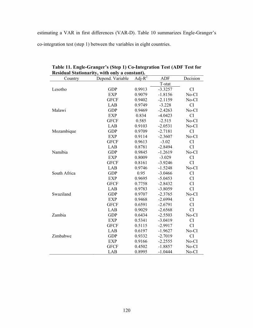
120
estimating a VAR in first differences (VAR-D). Table 10 summarizes Engle-Granger’s
co-integration test (step 1) between the variables in eight countries.
Table 11. Engle-Granger’s (Step 1) Co-Integration Test (ADF Test for Residual Stationarity, with only a constant).
Country Depend. Variable Adj-R2 ADF Decision T-stat
Lesotho GDP 0.9913 -3.3257 CI EXP 0.9079 -1.8156 No-CI GFCF 0.9402 -2.1159 No-CI LAB 0.9749 -3.228 CI Malawi GDP 0.9469 -2.4263 No-CI EXP 0.834 -4.0423 CI GFCF 0.585 -2.515 No-CI LAB 0.9103 -2.0531 No-CI Mozambique GDP 0.9709 -2.7181 CI EXP 0.9114 -2.3607 No-CI GFCF 0.9613 -3.02 CI LAB 0.8781 -2.8494 CI Namibia GDP 0.9845 -1.2619 No-CI EXP 0.8009 -3.029 CI GFCF 0.8161 -3.9246 CI LAB 0.9746 -1.5248 No-CI South Africa GDP 0.95 -3.0466 CI EXP 0.9695 -5.0453 CI GFCF 0.7758 -2.8432 CI LAB 0.9783 -3.8059 CI Swaziland GDP 0.9707 -2.3765 No-CI EXP 0.9468 -2.6994 CI GFCF 0.6591 -2.6791 CI LAB 0.9029 -2.6568 CI Zambia GDP 0.6434 -2.5503 No-CI EXP 0.5341 -3.0419 CI GFCF 0.5115 -2.9917 CI LAB 0.6197 -1.9627 No-CI Zimbabwe GDP 0.9332 -2.7019 CI EXP 0.9166 -2.2555 No-CI GFCF 0.4502 -1.8857 No-CI LAB 0.8995 -1.0444 No-CI

121
APPENDIX F
MODELS RESIDUAL DIAGNOSTICS
Table 12. Portmanteau Test For Cross Correlations of Residuals (Bi-variate Models with no exogenous Variables). Country Up to lags DF Chi-Square Pr > ChiSq Botswana 2 4 5.81 0.2136 3 8 6.44 0.5984 4 12 14.85 0.2496 Lesotho 5 4 21.09 0.0003 Malawi 3 4 3.26 0.5153 4 8 10.36 0.2409 Mozambique 3 4 2.27 0.6866 4 8 3.67 0.8860 Namibia 3 4 7.18 0.1268 4 8 9.46 0.3052 South Africa 5 4 15.24 0.0042 Swaziland 5 4 13.47 0.0092 Zambia 3 4 5.06 0.2816 4 8 5.99 0.6488 Zimbabwe 4 4 6.79 0.1472
Table 13. Jarque-Bera Normality Test, Univariate Model White Noise Diagnostics (with No Exogenous variables). Normality Country Variable DW ChiSq Prob>ChiSq Botswana DGDP 1.51 12.80 0.0017 LnEXP 1.76 2.18 0.3362 Lesotho LnGDP 2.05 0.68 0.7121 LnEXP 2.07 0.87 0.6457 Malawi LnGDP 2.04 0.13 0.9360 LnEXP 2.34 0.46 0.7932 Mozambique LnGDP 1.93 2.26 0.3236 LnEXP 2.10 4.19 0.1231 Namibia LnGDP 1.94 7.45 0.024 LnEXP 2.21 0.24 0.8879 South Africa LnGDP 1.88 1.06 0.5886 LnEXP 1.80 1.14 0.5661 Swaziland LnGDP 2.75 4.58 0.1011 LnEXP 1.85 0.33 0.8482 Zambia LnGDP 1.85 0.51 0.7764 LnEXP 1.79 2.56 0.278 Zimbabwe LnGDP 2.12 0.74 0.6890 LnEXP 1.95 1.58 0.4528

122
Table 14. Portmanteau Test For Cross Correlations of Residuals (with Exogenous Variables). Country Up to lags DF Chi-Square Pr > ChiSq Botswana 2 8 8.39 0.0784 3 8 9.11 0.3329 4 12 16.79 0.1577 Lesotho 2 4 9.51 0.0495 3 8 14.52 0.0693 4 12 22.21 0.0353 Malawi 2 4 5.12 0.2750 3 8 8.45 0.3905 4 12 16.37 0.1749 Mozambique 3 4 9.25 0.0550 4 8 12.72 0.1217 Namibia 2 4 8.52 0.0744 3 8 12.26 0.1402 4 12 14.47 0.2716 South Africa 2 4 18.25 0.0011 3 8 23.26 0.0030 4 12 28.91 0.0041 Swaziland 5 4 16.19 0.0028 Zambia 2 4 6.51 0.1639 3 8 11.10 0.1960 4 12 17.97 0.1167 Zimbabwe 2 4 9.10 0.0588 3 8 11.15 0.1932 4 12 20.96 0.0509
Table 15. Jarque-Bera Normality Test, Univariate Model White Noise Diagnostics (with Exogenous Models). Normality
Country Variable DW
ChiSq Prob>ChiSq
Botswana DGDP 1.58 5.83 0.0543 LnEXP 1.91 1.61 0.4474 Lesotho lnGDP 1.72 3.80 0.1496 LnEXP 2.30 0.35 0.8412 Malawi lnGDP 1.92 1.70 0.4273 LnEXP 1.66 0.44 0.8022 Mozambique lnGDP 2.57 1.11 0.5741 LnEXP 2.14 0.06 0.9722 Namibia lnGDP 2.34 5.54 0.0628 LnEXP 1.74 0.28 0.8685 South Africa lnGDP 1.42 0.76 0.6828 LnEXP 1.90 0.24 0.8859 Swaziland lnGDP 2.80 1.82 0.4022 LnEXP 1.93 1.79 0.4076 Zambia lnGDP 1.42 0.89 0.6403 LnEXP 2.02 2.06 0.3570 Zimbabwe lnGDP 1.57 0.89 0.6412 LnEXP 2.01 8.29 0.016

123
VITA
Ramona Sinoha-Lopete was born in Malabo, Equatorial Guinea. After completion
of high school in 1996 at Instituto Real Malabo, she matriculated at the University of
Equatorial Guinea (UNGE), in the college of Agriculture. She completed her technical
degree in 1999 and graduated as Technical Engineer in Agriculture and Animal Sciences.
She worked as a high school instructor for two years. In 2001, she was awarded a
scholarship from Chevron Equatorial Guinea in collaboration with her government and
UNGE to pursue postgraduate studies at Louisiana State University. She completed her
English Language Orientation program in 2002.
In order to meet Graduate School requirements, she completed a bachelor of
science in agricultural business in the Department of Agricultural Economics and
Agribusiness at Louisiana State University in 2004. Ramona Sinoha is now a candidate
for Master Degree in agricultural economics at Louisiana State University. She is looking
forward to pursuing a doctoral degree in agricultural economics.