Exporting, Licensing, FDI and Productivity Choice:

Theory and Evidence from Chilean Data*

Yiqing Xie †

Department of Economics

University of Colorado at Boulder

First Draft: May 2011This draft: November 8, 2011

*I’d like to thank my advisor, James Markusen, for his support, help and guidance. I

appreciate all the time and efforts of the members on my thesis committees:James Markusen,

Yongmin Chen, Keith Maskus, Thibault Fally. I also want to thank Luis Castro for kindly

offering me the Chilean data set. I am grateful to Cecilia Fieler, Loretta Fung, Wolfgang

Keller, Sylvain Leduc, Ben Li and Ken Teshima for helpful discussions; and the participants

at Canadian Economic Association and Western Economic Association for useful comments.

†Contact Info: yiqingxie@gmail.com, +1(720)2359107, http://spot.colorado.edu/˜xiey.

1

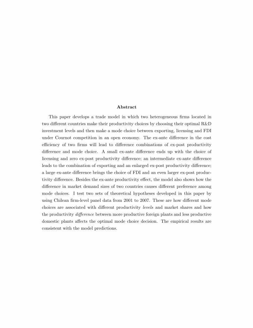
Abstract

This paper develops a trade model in which two heterogeneous firms located in

two different countries make their productivity choices by choosing their optimal R&D

investment levels and then make a mode choice between exporting, licensing and FDI

under Cournot competition in an open economy. The ex-ante difference in the cost

efficiency of two firms will lead to difference combinations of ex-post productivity

difference and mode choice. A small ex-ante difference ends up with the choice of

licensing and zero ex-post productivity difference; an intermediate ex-ante difference

leads to the combination of exporting and an enlarged ex-post productivity difference;

a large ex-ante difference brings the choice of FDI and an even larger ex-post produc-

tivity difference. Besides the ex-ante productivity effect, the model also shows how the

difference in market demand sizes of two countries causes different preference among

mode choices. I test two sets of theoretical hypotheses developed in this paper by

using Chilean firm-level panel data from 2001 to 2007. These are how different mode

choices are associated with different productivity levels and market shares and how

the productivity difference between more productive foreign plants and less productive

domestic plants affects the optimal mode choice decision. The empirical results are

consistent with the model predictions.

1 Introduction

Multinational firms have played a more and more important role in the world economy with

both international trade and foreign direct investment being fast growing economic activ-

ities. Many developing countries have liberalized their economies to attract foreign direct

investment (FDI) and licenses of foreign technology. On the other hand, firms also face the

problem that how they should sell their products in a more liberalized world market. This is

the mode choice for a firm. The mode choice means that a firm may choose one of the follow-

ing ways to serve the foreign market: exporting, licensing, or foreign direct investment1. A

firm’s optimal mode choice not only affects the profits of itself and its competitors, but also

has a large impact on the social welfare and technology improvement. The role that multi-

national firms play in the technological development has raised a lot of research interests and

has been studied theoretically and empirically through both self-selection channel and learn-

ing by exporting channel to reveal the relationship between trade behaviors and productivity.

This paper focuses on firms’ behaviors in the open economy. I develop a theoretical

model that combines mode choice with productivity choice of multinational firms. In the

open economy, firms can choose their R&D investment levels and thus productivity levels to

maximize their combined profits from domestic and foreign markets. At the same time, mode

choice between exporting, licensing and foreign direct investment (FDI) is also made. Foreign

direct investment in this paper refers to “horizontal” FDI which means that a firm acquires

a subsidiary in a foreign country to produce a final product purchased directly by consumers.

According to the theoretical model, two sets of interesting and testable theoretical hy-

potheses initiate the empirical study of the Chilean plant-level panel data. First, different

mode choices of a foreign firm play a different role in the productivity and intra-industry

allocation in the host country. Second, what ends up being an optimal mode choice is ac-

tually a result from the interactions between the more productive foreign firms and the less

productive domestic firms in the host country.

The existing theoretical work on the mode choice and productivity choice favors two

types of models. Monopolistic competition models which reveal the relationship between

productivity and mode choice usually assume that different productivity levels are exoge-

nously given (Helpman, Melitz and Yeaple 2004). Oligopolistic competition models which

apply Cournot competition use knowledge capital or human capital to differentiate firms

1FDI in this paper indicates horizontal foreign direct investment.

1

(Horstmann and Markusen 1987, Ethier and Markusen 1996) or allow firms to change R&D

investment levels to determine their productivity (Saggi 1999, Ghosh and Saha 2008). These

oligopolistic competition models usually focus on the competition in the country that has

relatively lower productivity firms or has no human capital.

In this paper, I introduce two heterogeneous firms (firm𝐻 and firm 𝐹 ) located in different

countries (country ℎ and country 𝑓). Firms are heterogeneous in their cost function efficiency

parameters (R&D investment to cost reduction transformability 𝜃 and base marginal cost

𝜂) which influence the returns from the R&D investment to the reduction of marginal cost.

Without loss of generality, I assume firm 𝐻 is the firm with a more efficient cost function

(lower base marginal cost and/or higher transformability from R&D investment to cost re-

duction). The model is a three-stage game. In the first stage, firm 𝐻 which has a more

efficient cost function makes its mode choice (exporting, licensing or FDI). Firm 𝐹 with a

less efficient marginal cost function accepts firm 𝐻’s mode choice according to the assump-

tions in the model. Under the exporting choice, both firms choose to serve both markets

(country ℎ and country 𝑓) and bear a symmetric iceberg trade cost when exporting. If firm

𝐻 prefers licensing, firm 𝐹 gets firm 𝐻’s technology and competes against firm 𝐻 in both

markets2. Neither firm 𝐻 nor firm 𝐹 is isolated from competition in either market (country

ℎ or country 𝑓). Under the FDI choice, firm 𝐻 pays a fixed cost and acquires a subsidiary

in country 𝑓 to avoid any other trade cost, while firm 𝐹 exports to country ℎ and still bears

the iceberg trade cost. Then in the second stage, two firms determine their corresponding

ex-post marginal costs by choosing their optimal R&D investment levels endogenously. In

the last stage (third stage) two firms compete against each other by choosing their optimal

output levels (Cournot duopoly competition) in both their domestic and foreign markets in

the open economy.

With a productivity level (marginal cost) endogenously chosen by the firm, this model

captures the relationship between productivity and mode choice in a more sophisticated way

compared to most monopolistic competition literature. Different from most oligopolistic

competition literature which only analyzes the effect of the mode choice on the host country,

the model in this paper is more realistic in considering the effect on the whole international

market (both host country and source country). This paper illustrates a model that combines

2I assume no exclusive licensing in either country. It is trivial that both firms will get the highest profitsand prefer licensing if I allow exclusive licensing since both firms can have monopoly power within its owncountry. In addition, exclusive licensing is not very credible assumption because among all three modechoices that a firm chooses to serve a foreign market, licensing is usually considered to give the licensorhaving the least control over the usage of its technology.

2

the features from some existing monopolistic competition and oligopolistic competition liter-

ature that includes intra-industry trade, endogenously productivity choice and mode choice.

The model in this paper emphasizes the joint determination of productivity and mode

choice of firms in the open economy by allowing firms to choose their ex-post marginal cost

(productivity) endogenously. The ex-ante difference between two firms is the difference in

their cost functions. Firm 𝐻 has a more efficient cost function with a lower base marginal

cost and/or higher transformability from R&D investment to reduction in marginal cost than

firm 𝐹 . If the ex-ante cost functions are similar for two firms, firm 𝐻 is more likely to prefer

licensing and the ex-post productivity difference of two firms disappears because licensing

will make both firms share the same ex-ante cost functions. With an intermediate ex-ante

difference in cost functions of two firms, firm 𝐻 prefers exporting most when it makes the

mode choice and the ex-post productivity difference determined by two firms’ productivity

choices is enlarged compared with the ex-ante difference. When the ex-ante difference in

cost functions of two firms gets large, firm 𝐻 is more likely to choose FDI and the ex-post

productivity difference of two firms is even larger than that in the exporting mode. The

interaction between productivity choice and mode choice studied in this paper offers a more

complete analysis of this relationship than most of the monopolistic competition literature.

This paper studies a bilateral trade that allows firms to compete in both domestic and

foreign markets. Firm 𝐹 with a less efficient cost function can still choose to export and

its productivity level under different mode choices that firm 𝐻 chooses. Under this assump-

tion, different from most oligopolistic competition literature, firm 𝐻 has to consider a more

complex competition effect caused by different mode choices because it cannot exclude com-

petition in its domestic market. Firm 𝐹 always prefers licensing to the other two mode

choices because licensing can offer this ex-ante less efficient firm a higher ex-post produc-

tivity level and a larger market share; however, licensing is not always firm 𝐻’s best mode

choice since the choice of licensing creates a most challenging ex-post competitor for firm H

in both countries. The total industry profit from two countries for two firms is not always

the highest under the licensing choice though I assume that firm 𝐻 can exact the entire

extra profit that firm 𝐹 can earn as licensing fee in the model. This is due to the dramatic

market price drop under this non-cooperative output competition game. By considering the

competition in both domestic market and foreign market, firm 𝐻 may choose any of the

modes under different circumstances.

The mode choice is not only interacted with the ex-post productivity choice but also

3

affected by the relative market demand size. This paper also includes a market size effect

on productivity and mode choices of firms by holding the world market size constant and

changing the relative size of two countries. Given the ex-ante cost efficiency difference is not

too large or too small to dominate the mode choice, the firm with better ex-ante cost effi-

ciency parameters (firm 𝐻) in a relatively smaller country (country ℎ) will probably choose

to license its technology to the other firm (firm 𝐹 ) located in a bigger market (country 𝑓).

The extra profit that firm 𝐹 can earn under the licensing choice (endogenous licensing fee)

is larger than firm 𝐻’s profit loss due to a larger trade cost saving effect for a larger market

size of country 𝑓 . With the relative market size of country ℎ increasing to an intermediate

level, FDI has a larger chance to occur for two reasons combined together. First, country 𝑓 ’s

market size is still large enough to make the variable exporting trade cost outweigh the fixed

FDI cost so that the FDI choice is preferred to the exporting choice. Second, the trade cost

saving effect of country 𝑓 decreases and the trade cost of exporting to country ℎ increases

under the licensing case, and hence licensing is no longer the optimal choice. As the relative

market size of country ℎ continues increasing, firm 𝐻 is more likely to directly export to the

relative smaller market of country 𝑓 because it is no longer worth spending a fixed FDI cost

to avoid the smaller amount of the variable trade cost.

There are quite a few empirical papers focusing on the interactions between export-

ing decision, mode choice and firm-level productivity. Clerides, Lach and Tybout(1998),

Pavcnik(2002), Helpman, Melitz and Yeaple(2004), Javorcik(2004), De Loecker(2007), Aw,

Roberts and Xu(2008) and Bustos(2011) have studied the effect of ex-ante firm-level pro-

ductivity on the exporting decision and mode choice (FDI or exporting) and the impact of

exporting decision and mode choice (FDI) on firms’ ex-post productivity levels in different

ways. Due to the lack of licensing information in most data set, licensing choice hasn’t been

well studied in the existing empirical literature.

In the empirical section of this paper, I use the Chilean plant-level panel data from 2001

to 2007 to study two sets of theoretical hypotheses.3 This data includes more than 5000

plants belonging to 111 different ISIC 4-digit manufacturing industries each year and the

information of both foreign linkages – licensing and FDI, which allows me to give a compari-

son of the effects on productivity and intra-industry allocations of different foreign linkages.

In addition, under what circumstance licensing or FDI will end up to be the optimal mode

3There is neither R&D investment variable nor enough switching observations from domestic plants toforeign subsidiaries or licensees in the data. Unfortunately I cannot observe/estimate a difference betweenthe ex-ante and the ex-post productivity as the theory part states in the paper.

4

choice can be studied.

As to the first set of theoretical hypotheses, foreign linkages including FDI and licensing

are positively correlated with the total factor productivity of a plant. Foreign subsidiaries

and domestic licensees on average show a higher productivity level than plants with no access

to foreign linkages. Moreover, foreign subsidiaries have an even higher average productivity

level compared with domestic licensees. Together with the basic productivity advantage

associated with foreign linkages, plants with access to foreign linkages (foreign subsidiaries

and domestic licensees) on average are also larger in size and have a larger market share

with respect to three plant-level dependent variables – total sales, value added and total

employment. Similarly, this intra-industry allocation effect of FDI is also larger than that

of licensing.

According to the second set of theoretical hypotheses, what determines the mode choice

is not the absolute productivity level of the more productive firm, but the productivity dif-

ference between more productive foreign firms and less productive domestic firms. A larger

average productivity difference between domestic Chilean plants and foreign subsidiaries

within an industry, which indicates a larger productivity advantage of relatively more pro-

ductive foreign firms, is associated with more foreign direct investment observed in the data.

If the productivity advantage of more productive foreign firms is smaller in an industry, more

licensing transactions are observed.

The following section (section 2) studies the interaction between productivity choice and

mode choice by holding the market demand sizes of two countries same. The initial (ex-

ante) difference in cost functions of two firms will end up with different productivity choices,

different mode choices, and different welfare situations for two countries. The assumption

of same market demand size is relaxed in section 3 so that relative market size of two coun-

tries is allowed to be different. I use one numerical example with different assumptions to

separate the ex-ante productivity effect by holding market sizes the same (section 2) from

the market size effect by fixing the cost functions (section 3) on the productivity choice and

mode choice. Given the Chilean data, I treat Chile as a host country and test two sets of

hypotheses generated from the theoretical model in section 4. The last section (section 5)

gives a brief conclusion of this paper.

5

2 (Ex-ante) Productivity Effect

2.1 Model Set-up

There are two countries ℎ and 𝑓 with the same domestic inverse demand function which is

𝑃 = 𝛼− 𝛽𝑋, (1)

where 𝑃 stands for the price of the good and 𝑋 for the quantity. In each country there is

a monopoly firm. Firm 𝐻 is the domestic firm for Country ℎ and firm 𝐹 is the domestic

firm for Country 𝑓 . In order to maximize its profit, each firm chooses its R&D investment

level first and then determines its marginal cost level by its given cost function. Firm 𝐻’s

marginal cost function is

𝑐𝐻 = 𝜂𝐻 − 𝜃𝐻𝐼12𝐻 , (2)

which captures the relationship between firm 𝐻’s marginal cost 𝑐𝐻 and its R&D investment

level 𝐼𝐻 with both 𝜂𝐻 and 𝜃𝐻 positive. 𝜂𝐻 is the base marginal cost (productivity) of firm 𝐻

and 𝜃𝐻 indicates the R&D investment to productivity transformability. The cost function

is more efficient if it has a smaller 𝜂𝐻 and a larger 𝜃𝐻 . With a higher R&D investment

level, firm 𝐻’s ex-post marginal cost level is lower, which means the productivity level of the

firm is higher. With more money invested in the R&D, the marginal cost is decreasing at a

diminishing rate. Similarly, firm 𝐹 ’s marginal cost function is

𝑐𝐹 = 𝜂𝐹 − 𝜃𝐹 𝐼12𝐹 . (3)

In the open economy, firm 𝐻 and 𝐹 which sell homogeneous goods compete by choosing

their optimal quantities (Cournot competition) in both country ℎ and country 𝑓 . I assume

firm 𝐻 has a more efficient cost function (smaller 𝜂 and larger 𝜃) compared with firm 𝐹

without loss of generality. There is a symmetric iceberg trade cost which equals 𝑡 if either

firm chooses to export to the other country4. Firm 𝐹 can pay a licensing fee (𝐿) to firm 𝐻

to get the same marginal cost function as firm 𝐻 and thus choose the same level of marginal

cost (productivity) as firm 𝐻. Firm 𝐻 can choose to incur a fixed investment 𝐷 (horizontal

FDI) in country 𝑓 so that it can sell goods to country 𝑓 directly without trade cost. Suppose

this fixed investment is large enough so that firm 𝐹 cannot afford the FDI cost due to its

less efficient cost function.

4The total marginal cost for firm 𝐻 to export one unit of its goods to country 𝑓 is 𝑐𝐻 + 𝑡.

6

There are three possible cases that might end up as equilibrium.5 First, both firms

choose to export to the other country with no licensing or FDI. In this situation, both firms

choose their optimal R&D investment levels interdependently and have different marginal

cost levels. Second, firm 𝐻 chooses to do FDI to get rid of the iceberg trade cost while firm

𝐹 chooses to export. In this case, they also have different cost levels due to their different

choices of R&D investment. Third, firm 𝐻 accepts the offer from firm 𝐹 and licenses its

production technology (more efficient marginal cost function) to firm 𝐹 . The licensing in

this paper is non-exclusive so that both firms will compete in both markets (country ℎ and

country 𝑓). After paying the licensing fee, firm 𝐹 gets the same marginal cost function from

firm 𝐻. Hence both firms will choose the same R&D investment level and enjoy the same

ex-post marginal cost.

In order to solve this model, I use a three-step backward induction process. In the

first step, I derive the intra-industry allocation results including output quantities, market

prices, profits and social welfares of two firms in two countries under all these three cases

given marginal costs of two firms (𝑐𝐻 and 𝑐𝐹 ). In the second step, I maximize the profits of

two firms by choosing their corresponding optimal R&D investment levels and thus deter-

mine the marginal costs under different cases. In the third step, the mode choice of firm 𝐻

can be determined by comparing the profits of these three cases.

2.1.1 Case 1 (Exporting):

Both firms compete against each other by choosing their optimal R&D investment in country

ℎ and 𝑓 separately. Firm 𝐻 has to incur an iceberg trade cost 𝑡 if it exports to country 𝑓 ,

while firm 𝐹 has to incur the same amount of trade cost 𝑡 if it sells in country ℎ. The model

reduces to a two-stage game given the mode choice is given as exporting. Both firms need

to choose their R&D investment levels and thus marginal cost levels first. Then they have

to figure out their best response functions in the Cournot competition and hence determine

their quantities, price and maximized profits.

By backward induction, suppose that both firms have decided their R&D investments

and marginal costs, their profit-maximizing quantities, price, mark-ups and profits can be

expressed as a function of their marginal costs as following. Superscript 𝐸 stands for the

5In the theoretical model, it is possible that more productive firm 𝐻 acquires less productive firm 𝐹and becomes a monopolist in the world market (both country ℎ and country 𝑓). However, in real life thereare usually either legal or political restrictions on M&A to exclude the possibility of this situation, so thispotential equilibrium will not be considered in this model.

7

exporting mode choice, and subscripts 𝐻 and 𝐹 indicate firm 𝐻 and firm 𝐹 , while subscripts

ℎ and 𝑓 stand for country ℎ and 𝑓 .

Quantities:

𝑋𝐸𝐻ℎ =

1

3𝛽

(𝛼− 2𝑐𝐸𝐻 + 𝑐𝐸𝐹 + 𝑡

), (4a)

𝑋𝐸𝐻𝑓 =

1

3𝛽

(𝛼− 2𝑐𝐸𝐻 + 𝑐𝐸𝐹 − 2𝑡

), (4b)

𝑋𝐸𝐹ℎ =

1

3𝛽

(𝛼− 2𝑐𝐸𝐹 + 𝑐𝐸𝐻 − 2𝑡

), (4c)

𝑋𝐸𝐹𝑓 =

1

3𝛽

(𝛼− 2𝑐𝐸𝐹 + 𝑐𝐸𝐻 + 𝑡

). (4d)

Prices: (same in both countries)

𝑃𝐸ℎ = 𝑃𝐸

𝑓 =1

3

(𝛼+ 𝑐𝐸𝐻 + 𝑐𝐸𝐹 + 𝑡

). (5)

Profits:

𝜋𝐸𝐻 =

1

9𝛽

(𝛼− 2𝑐𝐸𝐻 + 𝑐𝐸𝐹 + 𝑡

)2+

1

9𝛽

(𝛼− 2𝑐𝐸𝐻 + 𝑐𝐸𝐹 − 2𝑡

)2 − 𝐼𝐸𝐻 , (6a)

𝜋𝐸𝐹 =

1

9𝛽

(𝛼− 2𝑐𝐸𝐹 + 𝑐𝐸𝐻 + 𝑡

)2+

1

9𝛽

(𝛼− 2𝑐𝐸𝐹 + 𝑐𝐸𝐻 − 2𝑡

)2 − 𝐼𝐸𝐹 . (6b)

Welfares:

𝑤𝐸ℎ =

1

18𝛽

(2𝛼− 𝑐𝐸𝐻 − 𝑐𝐸𝐹 − 𝑡

)2+

1

9𝛽

(𝛼− 2𝑐𝐸𝐻 + 𝑐𝐸𝐹 + 𝑡

)2+

1

9𝛽

(𝛼− 2𝑐𝐸𝐻 + 𝑐𝐸𝐹 − 2𝑡

)2 − 𝐼𝐸𝐻 ,

(7a)

𝑤𝐸𝑓 =

1

18𝛽

(2𝛼− 𝑐𝐸𝐻 − 𝑐𝐸𝐹 − 𝑡

)2+

1

9𝛽

(𝛼− 2𝑐𝐸𝐹 + 𝑐𝐸𝐻 + 𝑡

)2+

1

9𝛽

(𝛼− 2𝑐𝐸𝐹 + 𝑐𝐸𝐻 − 2𝑡

)2 − 𝐼𝐸𝐹 .

(7b)

In order to maximize the profit, it is easy to determine the optimal R&D investment

levels and also calculate the marginal costs according to the cost functions.

𝐼𝐸𝐻 =

{4𝜃𝐻 [(9𝛽 − 12𝜃2𝐹 )𝛼− (18𝛽 − 12𝜃2𝐹 ) 𝜂𝐻 + 9𝛽𝜂𝐹 − (4.5𝛽 − 6𝜃2𝐹 )𝑡]

(9𝛽 − 8𝜃2𝐹 ) (9𝛽 − 8𝜃2𝐻)− 16𝜃2𝐻𝜃2𝐹

}2

, (8a)

8

𝐼𝐸𝐹 =

{4𝜃𝐹 [(9𝛽 − 12𝜃2𝐻)𝛼− (18𝛽 − 12𝜃2𝐻) 𝜂𝐹 + 9𝛽𝜂𝐻 − (4.5𝛽 − 6𝜃2𝐻)𝑡]

(9𝛽 − 8𝜃2𝐹 ) (9𝛽 − 8𝜃2𝐻)− 16𝜃2𝐻𝜃2𝐹

}2

. (8b)

And marginal cost levels are

𝑐𝐸𝐻 = 𝜂𝐻 − 𝜃𝐻

√𝐼𝐸𝐻 , (9a)

𝑐𝐸𝐹 = 𝜂𝐹 − 𝜃𝐹

√𝐼𝐸𝐹 . (9b)

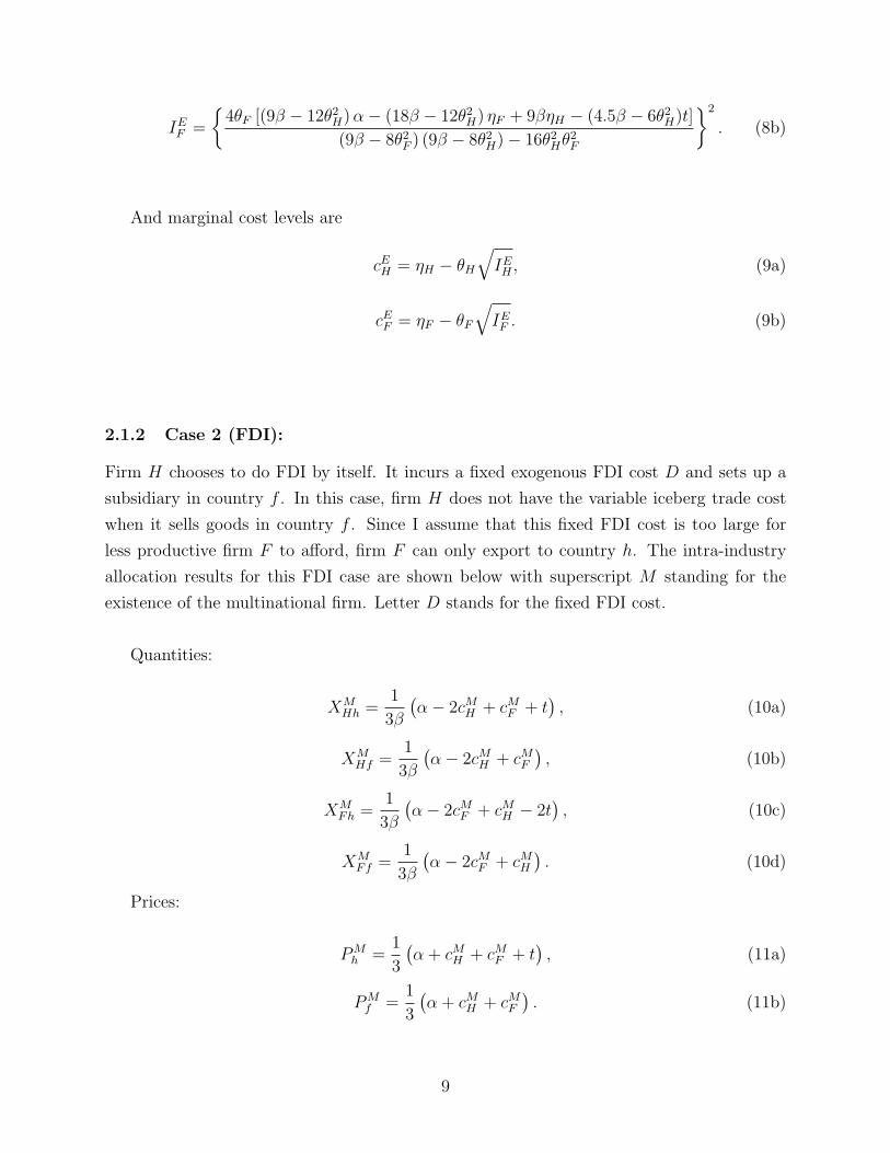
2.1.2 Case 2 (FDI):

Firm 𝐻 chooses to do FDI by itself. It incurs a fixed exogenous FDI cost 𝐷 and sets up a

subsidiary in country 𝑓 . In this case, firm 𝐻 does not have the variable iceberg trade cost

when it sells goods in country 𝑓 . Since I assume that this fixed FDI cost is too large for

less productive firm 𝐹 to afford, firm 𝐹 can only export to country ℎ. The intra-industry

allocation results for this FDI case are shown below with superscript 𝑀 standing for the

existence of the multinational firm. Letter 𝐷 stands for the fixed FDI cost.

Quantities:

𝑋𝑀𝐻ℎ =

1

3𝛽

(𝛼− 2𝑐𝑀𝐻 + 𝑐𝑀𝐹 + 𝑡

), (10a)

𝑋𝑀𝐻𝑓 =

1

3𝛽

(𝛼− 2𝑐𝑀𝐻 + 𝑐𝑀𝐹

), (10b)

𝑋𝑀𝐹ℎ =

1

3𝛽

(𝛼− 2𝑐𝑀𝐹 + 𝑐𝑀𝐻 − 2𝑡

), (10c)

𝑋𝑀𝐹𝑓 =

1

3𝛽

(𝛼− 2𝑐𝑀𝐹 + 𝑐𝑀𝐻

). (10d)

Prices:

𝑃𝑀ℎ =

1

3

(𝛼+ 𝑐𝑀𝐻 + 𝑐𝑀𝐹 + 𝑡

), (11a)

𝑃𝑀𝑓 =

1

3

(𝛼+ 𝑐𝑀𝐻 + 𝑐𝑀𝐹

). (11b)

9

Profits:

𝜋𝑀𝐻 =

1

9𝛽

(𝛼− 2𝑐𝑀𝐻 + 𝑐𝑀𝐹 + 𝑡

)2+

1

9𝛽

(𝛼− 2𝑐𝑀𝐻 + 𝑐𝑀𝐹

)2 − 𝐼𝑀𝐻 −𝐷, (12a)

𝜋𝑀𝐹 =

1

9𝛽

(𝛼− 2𝑐𝑀𝐹 + 𝑐𝑀𝐻

)2+

1

9𝛽

(𝛼− 2𝑐𝑀𝐹 + 𝑐𝑀𝐻 − 2𝑡

)2 − 𝐼𝑀𝐹 . (12b)

Welfares:

𝑤𝑀ℎ =

1

18𝛽

(2𝛼− 𝑐𝑀𝐻 − 𝑐𝑀𝐹 − 𝑡

)2+

1

9𝛽

(𝛼− 2𝑐𝑀𝐻 + 𝑐𝑀𝐹 + 𝑡

)2+

1

9𝛽

(𝛼− 2𝑐𝑀𝐻 + 𝑐𝑀𝐹

)2−𝐼𝑀𝐻 −𝐷,

(13a)

𝑤𝑀𝑓 =

1

18𝛽

(2𝛼− 𝑐𝑀𝐻 − 𝑐𝑀𝐹

)2+

1

9𝛽

(𝛼− 2𝑐𝑀𝐹 + 𝑐𝑀𝐻

)2+

1

9𝛽

(𝛼− 2𝑐𝑀𝐹 + 𝑐𝑀𝐻 − 2𝑡

)2−𝐼𝑀𝐹 . (13b)

The optimal R&D investment levels will be

𝐼𝑀𝐻 =

{4𝜃𝐻 [(9𝛽 − 12𝜃2𝐹 )𝛼− (18𝛽 − 12𝜃2𝐹 ) 𝜂𝐻 + 9𝛽𝜂𝐹 + 4.5𝛽𝑡]

(9𝛽 − 8𝜃2𝐹 ) (9𝛽 − 8𝜃2𝐻)− 16𝜃2𝐻𝜃2𝐹

}2

, (14a)

𝐼𝑀𝐹 =

{4𝜃𝐹 [(9𝛽 − 12𝜃2𝐻)𝛼− (18𝛽 − 12𝜃2𝐻) 𝜂𝐹 + 9𝛽𝜂𝐻 − (9𝛽 − 6𝜃2𝐻)𝑡]

(9𝛽 − 8𝜃2𝐹 ) (9𝛽 − 8𝜃2𝐻)− 16𝜃2𝐻𝜃2𝐹

}2

. (14b)

And marginal cost levels are

𝑐𝑀𝐻 = 𝜂𝐻 − 𝜃𝐻

√𝐼𝑀𝐻 , (15a)

𝑐𝑀𝐹 = 𝜂𝐹 − 𝜃𝐹

√𝐼𝑀𝐹 . (15b)

2.1.3 Case 3 (Licensing):

There are four assumptions in this model related with this licensing case that needs to be

stated. I have already mentioned the first assumption that firm 𝐻 is the firm with a more

efficient cost function without loss of generality, which means that firm 𝐻 has a smaller 𝜂

and a larger 𝜃 . If there is the optimal mode choice is licensing, firm 𝐻 should be the licenser

10

that licenses its production technology (more efficient cost function) to firm 𝐹 which is the

licensee.

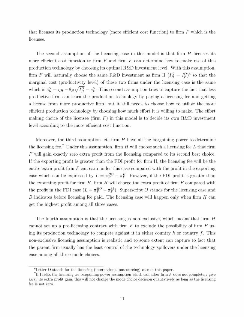
The second assumption of the licensing case in this model is that firm 𝐻 licenses its

more efficient cost function to firm 𝐹 and firm 𝐹 can determine how to make use of this

production technology by choosing its optimal R&D investment level. With this assumption,

firm 𝐹 will naturally choose the same R&D investment as firm H (𝐼𝑂𝐻 = 𝐼𝑂𝐹 )6 so that the

marginal cost (productivity level) of these two firms under the licensing case is the same

which is 𝑐𝑂𝐻 = 𝜂𝐻 − 𝜃𝐻√𝐼𝑂𝐻 = 𝑐𝑂𝐹 . This second assumption tries to capture the fact that less

productive firm can learn the production technology by paying a licensing fee and getting

a license from more productive firm, but it still needs to choose how to utilize the more

efficient production technology by choosing how much effort it is willing to make. The effort

making choice of the licensee (firm 𝐹 ) in this model is to decide its own R&D investment

level according to the more efficient cost function.

Moreover, the third assumption lets firm 𝐻 have all the bargaining power to determine

the licensing fee.7 Under this assumption, firm 𝐻 will choose such a licensing fee 𝐿 that firm

𝐹 will gain exactly zero extra profit from the licensing compared to its second best choice.

If the exporting profit is greater than the FDI profit for firm H, the licensing fee will be the

entire extra profit firm 𝐹 can earn under this case compared with the profit in the exporting

case which can be expressed by 𝐿 = 𝜋𝐵𝑂𝐹 − 𝜋𝐸

𝐹 . However, if the FDI profit is greater than

the exporting profit for firm 𝐻, firm 𝐻 will charge the extra profit of firm 𝐹 compared with

the profit in the FDI case (𝐿 = 𝜋𝐵𝑂𝐹 − 𝜋𝑀

𝐹 ). Superscript 𝑂 stands for the licensing case and

𝐵 indicates before licensing fee paid. The licensing case will happen only when firm 𝐻 can

get the highest profit among all three cases.

The fourth assumption is that the licensing is non-exclusive, which means that firm 𝐻

cannot set up a pre-licensing contract with firm 𝐹 to exclude the possibility of firm 𝐹 us-

ing its production technology to compete against it in either country ℎ or country 𝑓 . This

non-exclusive licensing assumption is realistic and to some extent can capture to fact that

the parent firm usually has the least control of the technology spillovers under the licensing

case among all three mode choices.

6Letter O stands for the licensing (international outsourcing) case in this paper.7If I relax the licensing fee bargaining power assumption which can allow firm 𝐹 does not completely give

away its extra profit gain, this will not change the mode choice decision qualitatively as long as the licensingfee is not zero.

11

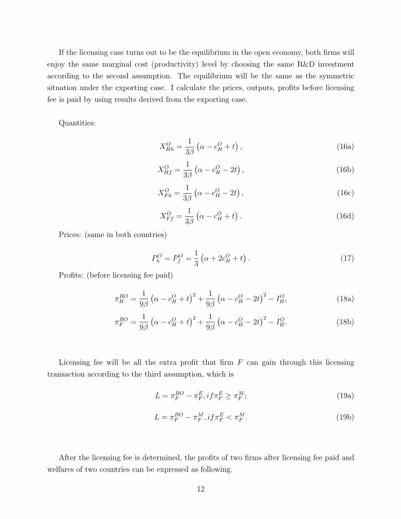
If the licensing case turns out to be the equilibrium in the open economy, both firms will

enjoy the same marginal cost (productivity) level by choosing the same R&D investment

according to the second assumption. The equilibrium will be the same as the symmetric

situation under the exporting case. I calculate the prices, outputs, profits before licensing

fee is paid by using results derived from the exporting case.

Quantities:

𝑋𝑂𝐻ℎ =

1

3𝛽

(𝛼− 𝑐𝑂𝐻 + 𝑡

), (16a)

𝑋𝑂𝐻𝑓 =

1

3𝛽

(𝛼− 𝑐𝑂𝐻 − 2𝑡

), (16b)

𝑋𝑂𝐹ℎ =

1

3𝛽

(𝛼− 𝑐𝑂𝐻 − 2𝑡

), (16c)

𝑋𝑂𝐹𝑓 =

1

3𝛽

(𝛼− 𝑐𝑂𝐻 + 𝑡

). (16d)

Prices: (same in both countries)

𝑃𝑂ℎ = 𝑃𝑂

𝑓 =1

3

(𝛼+ 2𝑐𝑂𝐻 + 𝑡

). (17)

Profits: (before licensing fee paid)

𝜋𝐵𝑂𝐻 =

1

9𝛽

(𝛼− 𝑐𝑂𝐻 + 𝑡

)2+

1

9𝛽

(𝛼− 𝑐𝑂𝐻 − 2𝑡

)2 − 𝐼𝑂𝐻 , (18a)

𝜋𝐵𝑂𝐹 =

1

9𝛽

(𝛼− 𝑐𝑂𝐻 + 𝑡

)2+

1

9𝛽

(𝛼− 𝑐𝑂𝐻 − 2𝑡

)2 − 𝐼𝑂𝐻 . (18b)

Licensing fee will be all the extra profit that firm 𝐹 can gain through this licensing

transaction according to the third assumption, which is

𝐿 = 𝜋𝐵𝑂𝐹 − 𝜋𝐸

𝐹 , 𝑖𝑓𝜋𝐸𝐹 ≥ 𝜋𝑀

𝐹 ; (19a)

𝐿 = 𝜋𝐵𝑂𝐹 − 𝜋𝑀

𝐹 , 𝑖𝑓𝜋𝐸𝐹 < 𝜋𝑀

𝐹 . (19b)

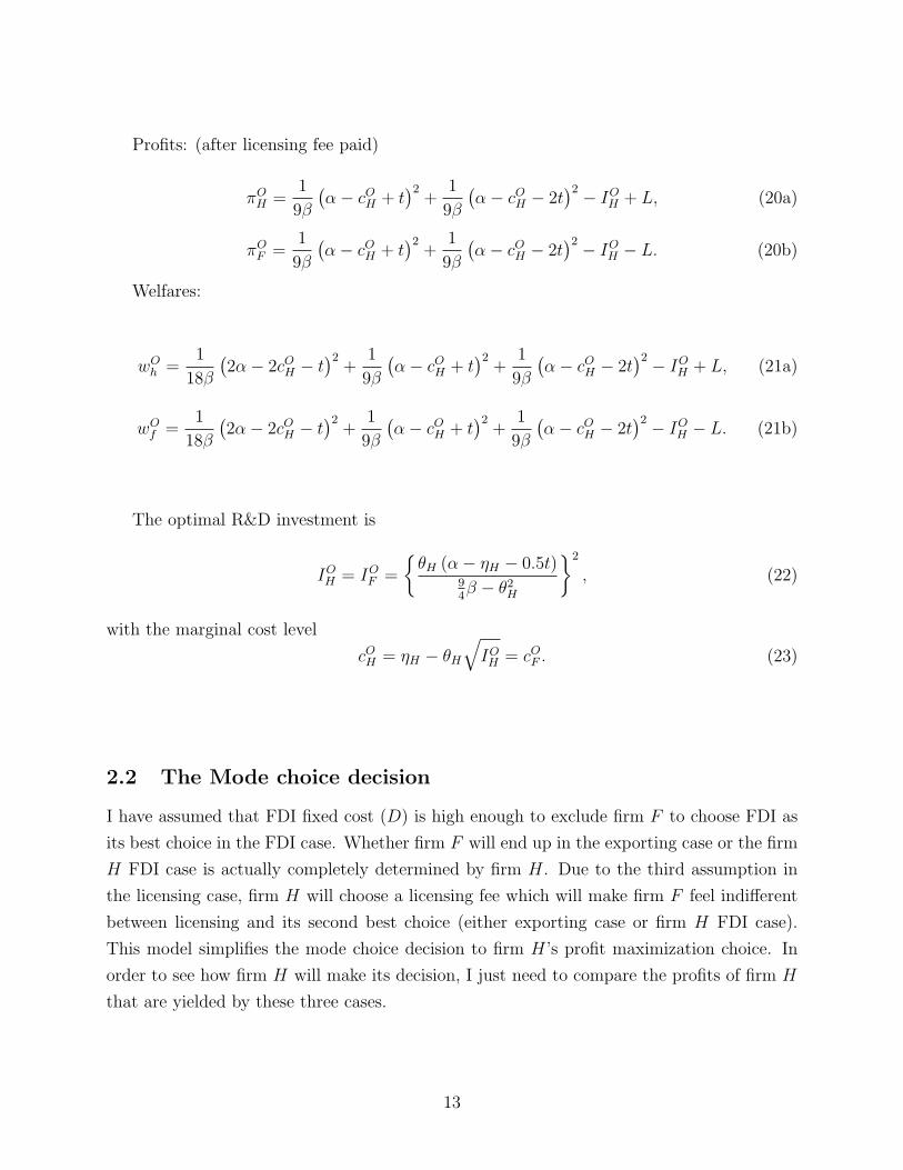
After the licensing fee is determined, the profits of two firms after licensing fee paid and

welfares of two countries can be expressed as following.

12

Profits: (after licensing fee paid)

𝜋𝑂𝐻 =

1

9𝛽

(𝛼− 𝑐𝑂𝐻 + 𝑡

)2+

1

9𝛽

(𝛼− 𝑐𝑂𝐻 − 2𝑡

)2 − 𝐼𝑂𝐻 + 𝐿, (20a)

𝜋𝑂𝐹 =

1

9𝛽

(𝛼− 𝑐𝑂𝐻 + 𝑡

)2+

1

9𝛽

(𝛼− 𝑐𝑂𝐻 − 2𝑡

)2 − 𝐼𝑂𝐻 − 𝐿. (20b)

Welfares:

𝑤𝑂ℎ =

1

18𝛽

(2𝛼− 2𝑐𝑂𝐻 − 𝑡

)2+

1

9𝛽

(𝛼− 𝑐𝑂𝐻 + 𝑡

)2+

1

9𝛽

(𝛼− 𝑐𝑂𝐻 − 2𝑡

)2 − 𝐼𝑂𝐻 + 𝐿, (21a)

𝑤𝑂𝑓 =

1

18𝛽

(2𝛼− 2𝑐𝑂𝐻 − 𝑡

)2+

1

9𝛽

(𝛼− 𝑐𝑂𝐻 + 𝑡

)2+

1

9𝛽

(𝛼− 𝑐𝑂𝐻 − 2𝑡

)2 − 𝐼𝑂𝐻 − 𝐿. (21b)

The optimal R&D investment is

𝐼𝑂𝐻 = 𝐼𝑂𝐹 =

{𝜃𝐻 (𝛼− 𝜂𝐻 − 0.5𝑡)

94𝛽 − 𝜃2𝐻

}2

, (22)

with the marginal cost level

𝑐𝑂𝐻 = 𝜂𝐻 − 𝜃𝐻

√𝐼𝑂𝐻 = 𝑐𝑂𝐹 . (23)

2.2 The Mode choice decision

I have assumed that FDI fixed cost (𝐷) is high enough to exclude firm 𝐹 to choose FDI as

its best choice in the FDI case. Whether firm 𝐹 will end up in the exporting case or the firm

𝐻 FDI case is actually completely determined by firm 𝐻. Due to the third assumption in

the licensing case, firm 𝐻 will choose a licensing fee which will make firm 𝐹 feel indifferent

between licensing and its second best choice (either exporting case or firm 𝐻 FDI case).

This model simplifies the mode choice decision to firm 𝐻’s profit maximization choice. In

order to see how firm 𝐻 will make its decision, I just need to compare the profits of firm 𝐻

that are yielded by these three cases.

13

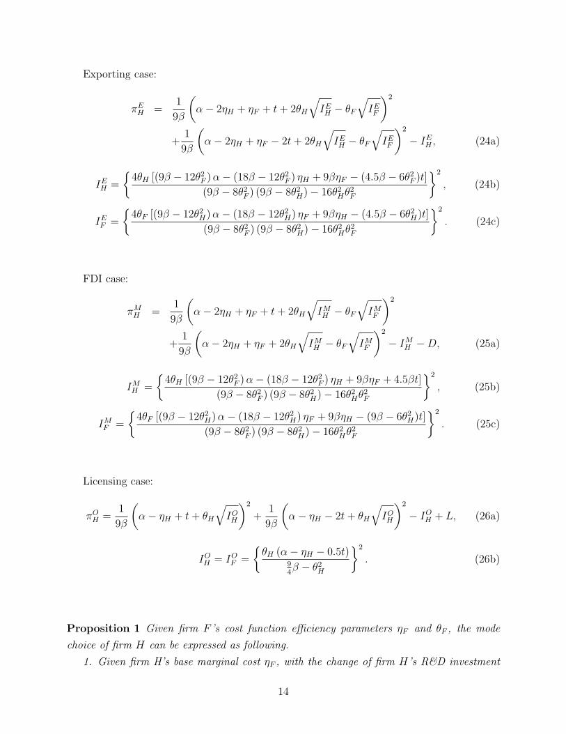
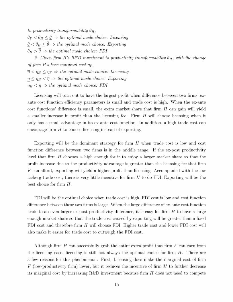
Exporting case:

𝜋𝐸𝐻 =

1

9𝛽

(𝛼− 2𝜂𝐻 + 𝜂𝐹 + 𝑡+ 2𝜃𝐻

√𝐼𝐸𝐻 − 𝜃𝐹

√𝐼𝐸𝐹

)2

+1

9𝛽

(𝛼− 2𝜂𝐻 + 𝜂𝐹 − 2𝑡+ 2𝜃𝐻

√𝐼𝐸𝐻 − 𝜃𝐹

√𝐼𝐸𝐹

)2

− 𝐼𝐸𝐻 , (24a)

𝐼𝐸𝐻 =

{4𝜃𝐻 [(9𝛽 − 12𝜃2𝐹 )𝛼− (18𝛽 − 12𝜃2𝐹 ) 𝜂𝐻 + 9𝛽𝜂𝐹 − (4.5𝛽 − 6𝜃2𝐹 )𝑡]

(9𝛽 − 8𝜃2𝐹 ) (9𝛽 − 8𝜃2𝐻)− 16𝜃2𝐻𝜃2𝐹

}2

, (24b)

𝐼𝐸𝐹 =

{4𝜃𝐹 [(9𝛽 − 12𝜃2𝐻)𝛼− (18𝛽 − 12𝜃2𝐻) 𝜂𝐹 + 9𝛽𝜂𝐻 − (4.5𝛽 − 6𝜃2𝐻)𝑡]

(9𝛽 − 8𝜃2𝐹 ) (9𝛽 − 8𝜃2𝐻)− 16𝜃2𝐻𝜃2𝐹

}2

. (24c)

FDI case:

𝜋𝑀𝐻 =

1

9𝛽

(𝛼− 2𝜂𝐻 + 𝜂𝐹 + 𝑡+ 2𝜃𝐻

√𝐼𝑀𝐻 − 𝜃𝐹

√𝐼𝑀𝐹

)2

+1

9𝛽

(𝛼− 2𝜂𝐻 + 𝜂𝐹 + 2𝜃𝐻

√𝐼𝑀𝐻 − 𝜃𝐹

√𝐼𝑀𝐹

)2

− 𝐼𝑀𝐻 −𝐷, (25a)

𝐼𝑀𝐻 =

{4𝜃𝐻 [(9𝛽 − 12𝜃2𝐹 )𝛼− (18𝛽 − 12𝜃2𝐹 ) 𝜂𝐻 + 9𝛽𝜂𝐹 + 4.5𝛽𝑡]

(9𝛽 − 8𝜃2𝐹 ) (9𝛽 − 8𝜃2𝐻)− 16𝜃2𝐻𝜃2𝐹

}2

, (25b)

𝐼𝑀𝐹 =

{4𝜃𝐹 [(9𝛽 − 12𝜃2𝐻)𝛼− (18𝛽 − 12𝜃2𝐻) 𝜂𝐹 + 9𝛽𝜂𝐻 − (9𝛽 − 6𝜃2𝐻)𝑡]

(9𝛽 − 8𝜃2𝐹 ) (9𝛽 − 8𝜃2𝐻)− 16𝜃2𝐻𝜃2𝐹

}2

. (25c)

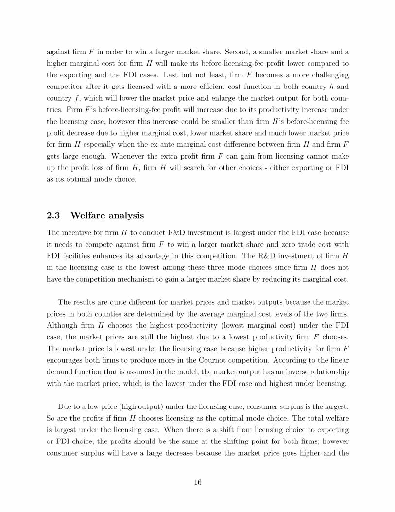
Licensing case:

𝜋𝑂𝐻 =

1

9𝛽

(𝛼− 𝜂𝐻 + 𝑡+ 𝜃𝐻

√𝐼𝑂𝐻

)2

+1

9𝛽

(𝛼− 𝜂𝐻 − 2𝑡+ 𝜃𝐻

√𝐼𝑂𝐻

)2

− 𝐼𝑂𝐻 + 𝐿, (26a)

𝐼𝑂𝐻 = 𝐼𝑂𝐹 =

{𝜃𝐻 (𝛼− 𝜂𝐻 − 0.5𝑡)

94𝛽 − 𝜃2𝐻

}2

. (26b)

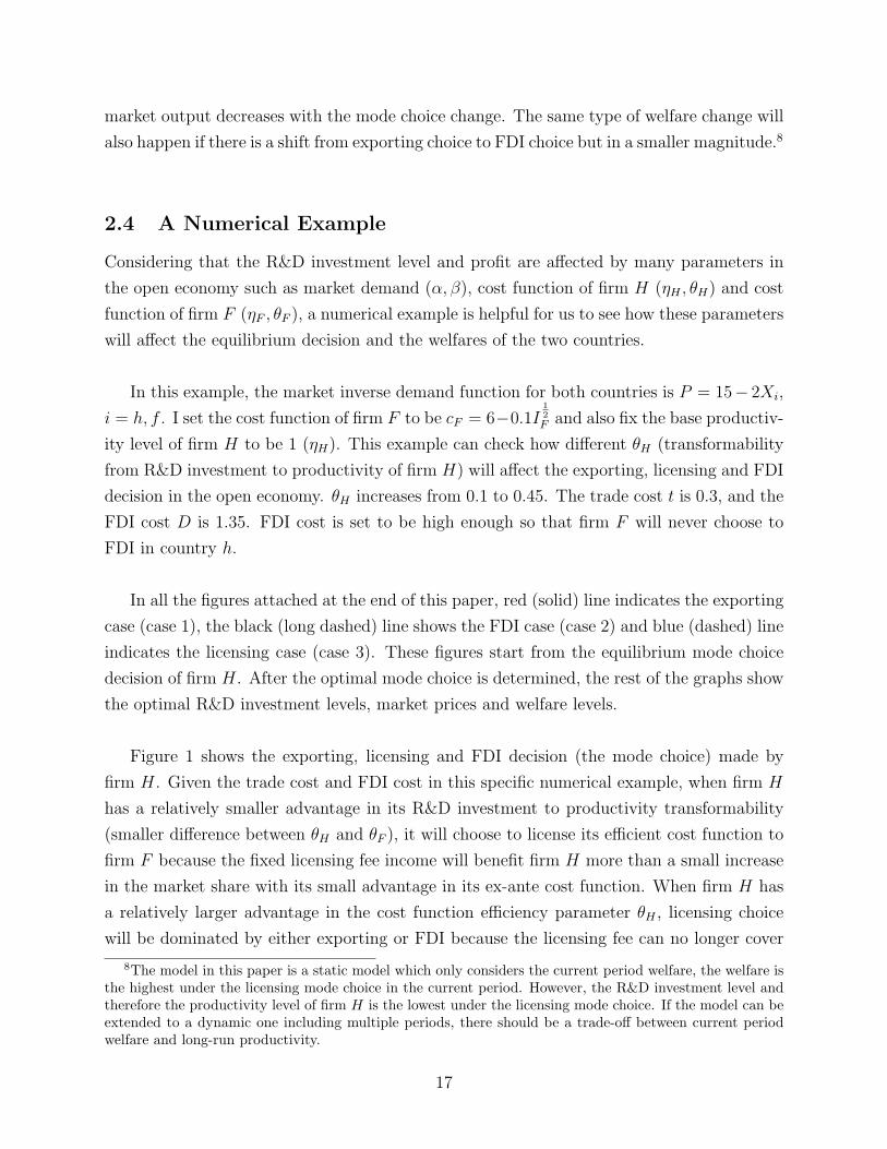
Proposition 1 Given firm 𝐹 ’s cost function efficiency parameters 𝜂𝐹 and 𝜃𝐹 , the mode

choice of firm 𝐻 can be expressed as following.

1. Given firm H’s base marginal cost 𝜂𝐹 , with the change of firm 𝐻’s R&D investment

14

to productivity transformability 𝜃𝐻 ,

𝜃𝐹 < 𝜃𝐻 ≤ 𝜃 ⇒ the optimal mode choice: Licensing

𝜃 < 𝜃𝐻 ≤ 𝜃 ⇒ the optimal mode choice: Exporting

𝜃𝐻 > 𝜃 ⇒ the optimal mode choice: FDI

2. Given firm H’s R&D investment to productivity transformability 𝜃𝐻 , with the change

of firm H’s base marginal cost 𝜂𝐹 ,

𝜂 < 𝜂𝐻 ≤ 𝜂𝐹 ⇒ the optimal mode choice: Licensing

𝜂 ≤ 𝜂𝐻 < 𝜂 ⇒ the optimal mode choice: Exporting

𝜂𝐻 < 𝜂 ⇒ the optimal mode choice: FDI

Licensing will turn out to have the largest profit when difference between two firms’ ex-

ante cost function efficiency parameters is small and trade cost is high. When the ex-ante

cost functions’ difference is small, the extra market share that firm 𝐻 can gain will yield

a smaller increase in profit than the licensing fee. Firm 𝐻 will choose licensing when it

only has a small advantage in its ex-ante cost function. In addition, a high trade cost can

encourage firm 𝐻 to choose licensing instead of exporting.

Exporting will be the dominant strategy for firm 𝐻 when trade cost is low and cost

function difference between two firms is in the middle range. If the ex-post productivity

level that firm 𝐻 chooses is high enough for it to enjoy a larger market share so that the

profit increase due to the productivity advantage is greater than the licensing fee that firm

𝐹 can afford, exporting will yield a higher profit than licensing. Accompanied with the low

iceberg trade cost, there is very little incentive for firm 𝐻 to do FDI. Exporting will be the

best choice for firm 𝐻.

FDI will be the optimal choice when trade cost is high, FDI cost is low and cost function

difference between these two firms is large. When the large difference of ex-ante cost function

leads to an even larger ex-post productivity difference, it is easy for firm 𝐻 to have a large

enough market share so that the trade cost caused by exporting will be greater than a fixed

FDI cost and therefore firm 𝐻 will choose FDI. Higher trade cost and lower FDI cost will

also make it easier for trade cost to outweigh the FDI cost.

Although firm 𝐻 can successfully grab the entire extra profit that firm 𝐹 can earn from

the licensing case, licensing is still not always the optimal choice for firm 𝐻. There are

a few reasons for this phenomenon. First, Licensing does make the marginal cost of firm

𝐹 (low-productivity firm) lower, but it reduces the incentive of firm 𝐻 to further decrease

its marginal cost by increasing R&D investment because firm 𝐻 does not need to compete

15

against firm 𝐹 in order to win a larger market share. Second, a smaller market share and a

higher marginal cost for firm 𝐻 will make its before-licensing-fee profit lower compared to

the exporting and the FDI cases. Last but not least, firm 𝐹 becomes a more challenging

competitor after it gets licensed with a more efficient cost function in both country ℎ and

country 𝑓 , which will lower the market price and enlarge the market output for both coun-

tries. Firm 𝐹 ’s before-licensing-fee profit will increase due to its productivity increase under

the licensing case, however this increase could be smaller than firm 𝐻’s before-licensing fee

profit decrease due to higher marginal cost, lower market share and much lower market price

for firm 𝐻 especially when the ex-ante marginal cost difference between firm 𝐻 and firm 𝐹

gets large enough. Whenever the extra profit firm 𝐹 can gain from licensing cannot make

up the profit loss of firm 𝐻, firm 𝐻 will search for other choices - either exporting or FDI

as its optimal mode choice.

2.3 Welfare analysis

The incentive for firm 𝐻 to conduct R&D investment is largest under the FDI case because

it needs to compete against firm 𝐹 to win a larger market share and zero trade cost with

FDI facilities enhances its advantage in this competition. The R&D investment of firm 𝐻

in the licensing case is the lowest among these three mode choices since firm 𝐻 does not

have the competition mechanism to gain a larger market share by reducing its marginal cost.

The results are quite different for market prices and market outputs because the market

prices in both counties are determined by the average marginal cost levels of the two firms.

Although firm 𝐻 chooses the highest productivity (lowest marginal cost) under the FDI

case, the market prices are still the highest due to a lowest productivity firm 𝐹 chooses.

The market price is lowest under the licensing case because higher productivity for firm 𝐹

encourages both firms to produce more in the Cournot competition. According to the linear

demand function that is assumed in the model, the market output has an inverse relationship

with the market price, which is the lowest under the FDI case and highest under licensing.

Due to a low price (high output) under the licensing case, consumer surplus is the largest.

So are the profits if firm 𝐻 chooses licensing as the optimal mode choice. The total welfare

is largest under the licensing case. When there is a shift from licensing choice to exporting

or FDI choice, the profits should be the same at the shifting point for both firms; however

consumer surplus will have a large decrease because the market price goes higher and the

16

market output decreases with the mode choice change. The same type of welfare change will

also happen if there is a shift from exporting choice to FDI choice but in a smaller magnitude.8

2.4 A Numerical Example

Considering that the R&D investment level and profit are affected by many parameters in

the open economy such as market demand (𝛼, 𝛽), cost function of firm 𝐻 (𝜂𝐻 , 𝜃𝐻) and cost

function of firm 𝐹 (𝜂𝐹 , 𝜃𝐹 ), a numerical example is helpful for us to see how these parameters

will affect the equilibrium decision and the welfares of the two countries.

In this example, the market inverse demand function for both countries is 𝑃 = 15− 2𝑋𝑖,

𝑖 = ℎ, 𝑓 . I set the cost function of firm 𝐹 to be 𝑐𝐹 = 6−0.1𝐼12𝐹 and also fix the base productiv-

ity level of firm 𝐻 to be 1 (𝜂𝐻). This example can check how different 𝜃𝐻 (transformability

from R&D investment to productivity of firm 𝐻) will affect the exporting, licensing and FDI

decision in the open economy. 𝜃𝐻 increases from 0.1 to 0.45. The trade cost 𝑡 is 0.3, and the

FDI cost 𝐷 is 1.35. FDI cost is set to be high enough so that firm 𝐹 will never choose to

FDI in country ℎ.

In all the figures attached at the end of this paper, red (solid) line indicates the exporting

case (case 1), the black (long dashed) line shows the FDI case (case 2) and blue (dashed) line

indicates the licensing case (case 3). These figures start from the equilibrium mode choice

decision of firm 𝐻. After the optimal mode choice is determined, the rest of the graphs show

the optimal R&D investment levels, market prices and welfare levels.

Figure 1 shows the exporting, licensing and FDI decision (the mode choice) made by

firm 𝐻. Given the trade cost and FDI cost in this specific numerical example, when firm 𝐻

has a relatively smaller advantage in its R&D investment to productivity transformability

(smaller difference between 𝜃𝐻 and 𝜃𝐹 ), it will choose to license its efficient cost function to

firm 𝐹 because the fixed licensing fee income will benefit firm 𝐻 more than a small increase

in the market share with its small advantage in its ex-ante cost function. When firm 𝐻 has

a relatively larger advantage in the cost function efficiency parameter 𝜃𝐻 , licensing choice

will be dominated by either exporting or FDI because the licensing fee can no longer cover

8The model in this paper is a static model which only considers the current period welfare, the welfare isthe highest under the licensing mode choice in the current period. However, the R&D investment level andtherefore the productivity level of firm 𝐻 is the lowest under the licensing mode choice. If the model can beextended to a dynamic one including multiple periods, there should be a trade-off between current periodwelfare and long-run productivity.

17

the profit decrease of firm 𝐻 due to the market share decrease, marginal cost increase and

market price decrease under the licensing case. When firm 𝐻 is very efficient in transforming

R&D investment to productivity, it will choose to conduct foreign direct investment because

it can gain a large foreign market share and hence forgoing a fixed FDI cost can make it get

rid of the high total trade cost. Firm 𝐻 will just choose to export to country 𝐹 when R&D

investment to productivity transformability is in the middle range, which means that larger

the market share, higher the market price and lower the marginal cost together is better

than the fixed licensing fee while the foreign market share is not large enough for the trade

cost to outweigh the fixed FDI cost.

The following two figures (figure 2 and figure 3) present the R&D invesment choices for

two firms under different optimal mode choices. FDI case is associated with the highest

R&D investment choice for firm 𝐻 while the licensing case relates with the lowest invest-

ment choice for firm 𝐻, which is just the opposite to the choices of firm 𝐹 . Firm 𝐹 ’s R&D

invesment, which is the same as firm 𝐻’s under the licensing choice, is much larger than the

R&D investment under other two mode choices. Figure 3 only has two segments for export-

ing and FDI for firm 𝐹 in order to graph a more clear trend of these two mode choices. In

figure 2, there are two jumps - both happen when there is a mode choice shift. The first

jump happens when firm 𝐻 shifts from licensing to exporting. Licensing actually discour-

ages firm 𝐻 to reduce its marginal cost compared with exporting or FDI because there is no

such competition mechanism for firm 𝐻 to invest more R&D in order to win a larger market

share. The second jump shows up when firm 𝐻 starts to choose FDI instead of exporting.

The magnitude of this jump is much smaller than that of the previous one since the compe-

tition mechanism to win a larger market share is the same for both exporting and FDI cases.

The elimination of trade cost for firm 𝐻 due to FDI enhances the easiness for firm 𝐻 to win

a larger market share in country 𝑓 and therefore induces this upward R&D investment jump.

Figure 4 and figure 5 show the market prices in each country. In this model, prices are

the same for both countries under the licensing and exporting choices. And consumers in

country 𝑓 enjoy a lower market price than those in country ℎ under the FDI choice because

of the elimination of iceberg trade cost when firm 𝐻 sells its product in country 𝑓 . The

market price is highest for the exporting case and lowest under the licensing case for both

countries. The price jump caused by the shift from licensing choice to exporting choice is

large in magnitude for both countries because the increase in the productivity level (decrease

in the marginal cost) of firm 𝐹 under the licensing choice enhances the competitiveness in

this duopoly market, enlarges the total market output and thus reduces the market price

18

a lot. The jump between exporting and FDI choices is relatively smaller with an even less

obvious change in country ℎ because the price decrease under FDI choice is mainly caused

by the higher productivity choice by firm 𝐻 and FDI can only happen in country 𝑓 by firm

𝐻 so that consumers in country 𝑓 benefit more with a larger price decrease and a larger

market output increase.

Figure 6 and 7 show the welfares under the optimal mode choice determined by firm 𝐻.

Similar to the previous figures, there are also two jumps of welfares in both countries showing

up at the mode choice shifting points. The first large welfare decrease is from the licensing

choice to the exporting choice. Welfare is the highest for both countries under the licensing

choice because the lower price and the higher output largely increase the consumer surplus.

At this first mode choice shifting point, the profits generated under the licensing choice and

exporting choice are the same, so the decrease in total welfare is completely caused by the

loss in the consumer surplus due to an increase in market price (a decrease in market output)

shown by figure 4 and 5. Welfare increases when there is a shift from exporting choice to

FDI choice for both country ℎ and country 𝑓 , and the welfare increase for country ℎ from

this mode choice change is very small. At the mode choice shifting point, again there is no

profit change for either firm 𝐻 or firm 𝐹 . Consumers in country ℎ still have to bear the

trade cost so that their consumer surplus gain is small which is purely caused by a higher

productivity choice of firm 𝐻. Welfare has a more obvious increase from this second mode

choice change for country 𝑓 because besides a higher productivity choice of firm 𝐻, the

consumers no longer need to pay any trade cost in country 𝑓 .

3 Market Size Effect

3.1 Model Set-up

In this section, I release the symmetric demand assumption to allow two countries ℎ and 𝑓

to have different domestic inverse demand functions which are

𝑃𝑖 = 𝛼− 𝛽𝑖𝑋𝑖, 𝑖 = ℎ, 𝑓, (27)

where 𝑃𝑖 stands for the price of the good in country 𝑖 and 𝑋𝑖 for the market quantity of

country 𝑖. The consumers of both countries have the same choke price for the good which is

𝛼. At the same price, the price elasticities of demand for both demand curves are also the

same. Different 𝛽 indicates different market demand size (no. of consumers). A smaller 𝛽 is

19

associated with a larger market demand size.

In the open economy, the optimal R&D investment levels, marginal costs, market out-

puts, prices, profits and welfares under different mode choices will have the following results.

The notations have the same meanings as those in section 2.

3.1.1 Case 1 (Exporting):

R&D investments:

𝐼𝐸𝐻 =

{4𝜃𝐻 [(4.5𝐵 − 3𝜃2𝐹 )𝛼− (9𝐵 − 3𝜃2𝐹 ) 𝜂𝐻 + 4.5𝐵𝜂𝐹 − (4.5𝐵(2𝛽ℎ − 𝛽𝑓 )− 3𝜃2𝐹2𝛽ℎ)𝑡/(𝛽𝑓 + 𝛽ℎ)]

(9𝐵 − 4𝜃2𝐹 ) (9𝐵 − 4𝜃2𝐻)− 4𝜃2𝐻𝜃2𝐹

}2

,

(28a)

𝐼𝐸𝐻 =

{4𝜃𝐹 [(4.5𝐵 − 3𝜃2𝐻)𝛼− (9𝐵 − 3𝜃2𝐻) 𝜂𝐹 + 4.5𝐵𝜂𝐻 − (4.5𝐵(2𝛽𝑓 − 𝛽ℎ)− 3𝜃2𝐻2𝛽𝑓 )𝑡/(𝛽𝑓 + 𝛽ℎ)]

(9𝐵 − 4𝜃2𝐹 ) (9𝐵 − 4𝜃2𝐻)− 4𝜃2𝐻𝜃2𝐹

}2

,

(28b)

where:

𝐵 =𝛽ℎ𝛽𝑓

𝛽ℎ + 𝛽𝑓

. (29)

Marginal costs:

𝑐𝐸𝐻 = 𝜂𝐻 − 𝜃𝐻

√𝐼𝐸𝐻 , (30a)

𝑐𝐸𝐹 = 𝜂𝐹 − 𝜃𝐹

√𝐼𝐸𝐹 . (30b)

Quantities:

𝑋𝐸𝐻ℎ =

1

3𝛽ℎ

(𝛼− 2𝑐𝐸𝐻 + 𝑐𝐸𝐹 + 𝑡

), (31a)

𝑋𝐸𝐻𝑓 =

1

3𝛽𝑓

(𝛼− 2𝑐𝐸𝐻 + 𝑐𝐸𝐹 − 2𝑡

), (31b)

𝑋𝐸𝐹ℎ =

1

3𝛽ℎ

(𝛼− 2𝑐𝐸𝐹 + 𝑐𝐸𝐻 − 2𝑡

), (31c)

𝑋𝐸𝐹𝑓 =

1

3𝛽𝑓

(𝛼− 2𝑐𝐸𝐹 + 𝑐𝐸𝐻 + 𝑡

). (31d)

Prices: (same in both countries)

𝑃𝐸ℎ = 𝑃𝐸

𝑓 =1

3

(𝛼+ 𝑐𝐸𝐻 + 𝑐𝐸𝐹 + 𝑡

). (32)

20

Profits:

𝜋𝐸𝐻 =

1

9𝛽ℎ

(𝛼− 2𝑐𝐸𝐻 + 𝑐𝐸𝐹 + 𝑡

)2+

1

9𝛽𝑓

(𝛼− 2𝑐𝐸𝐻 + 𝑐𝐸𝐹 − 2𝑡

)2 − 𝐼𝐸𝐻 , (33a)

𝜋𝐸𝐹 =

1

9𝛽𝑓

(𝛼− 2𝑐𝐸𝐹 + 𝑐𝐸𝐻 + 𝑡

)2+

1

9𝛽ℎ

(𝛼− 2𝑐𝐸𝐹 + 𝑐𝐸𝐻 − 2𝑡

)2 − 𝐼𝐸𝐹 . (33b)

Welfares:

𝑤𝐸ℎ =

1

18𝛽ℎ

(2𝛼− 𝑐𝐸𝐻 − 𝑐𝐸𝐹 − 𝑡

)2+

1

9𝛽ℎ

(𝛼− 2𝑐𝐸𝐻 + 𝑐𝐸𝐹 + 𝑡

)2+

1

9𝛽𝑓

(𝛼− 2𝑐𝐸𝐻 + 𝑐𝐸𝐹 − 2𝑡

)2−𝐼𝐸𝐻 ,

(34a)

𝑤𝐸𝑓 =

1

18𝛽𝑓

(2𝛼− 𝑐𝐸𝐻 − 𝑐𝐸𝐹 − 𝑡

)2+

1

9𝛽𝑓

(𝛼− 2𝑐𝐸𝐹 + 𝑐𝐸𝐻 + 𝑡

)2+

1

9𝛽ℎ

(𝛼− 2𝑐𝐸𝐹 + 𝑐𝐸𝐻 − 2𝑡

)2−𝐼𝐸𝐹 .

(34b)

3.1.2 Case 2 (FDI):

R&D investments:

𝐼𝑀𝐻 =

{4𝜃𝐻 [(4.5𝐵 − 3𝜃2𝐹 )𝛼− (9𝐵 − 3𝜃2𝐹 ) 𝜂𝐻 + 4.5𝐵𝜂𝐹 + (4.5𝐵/𝛽ℎ − 2𝜃2𝐹/𝛽ℎ + 2𝜃2𝐹/𝛽𝑓 )𝐵𝑡]

(9𝐵 − 4𝜃2𝐹 ) (9𝐵 − 4𝜃2𝐻)− 4𝜃2𝐻𝜃2𝐹

}2

,

(35a)

𝐼𝑀𝐹 =

{4𝜃𝐹 [(4.5𝐵 − 3𝜃2𝐻)𝛼− (9𝐵 − 3𝜃2𝐻) 𝜂𝐹 + 4.5𝐵𝜂𝐻 − (9𝐵/𝛽𝑓 − 4𝜃2𝐻/𝛽𝑓 + 𝜃2𝐻/𝛽ℎ)𝐵𝑡]

(9𝐵 − 4𝜃2𝐹 ) (9𝐵 − 4𝜃2𝐻)− 4𝜃2𝐻𝜃2𝐹

}2

,

(35b)

where:

𝐵 =𝛽ℎ𝛽𝑓

𝛽ℎ + 𝛽𝑓

. (36)

Marginal costs:

𝑐𝑀𝐻 = 𝜂𝐻 − 𝜃𝐻

√𝐼𝑀𝐻 , (37a)

𝑐𝑀𝐹 = 𝜂𝐹 − 𝜃𝐹

√𝐼𝑀𝐹 . (37b)

Quantities:

𝑋𝑀𝐻ℎ =

1

3𝛽ℎ

(𝛼− 2𝑐𝑀𝐻 + 𝑐𝑀𝐹 + 𝑡

), (38a)

21

𝑋𝑀𝐻𝑓 =

1

3𝛽𝑓

(𝛼− 2𝑐𝑀𝐻 + 𝑐𝑀𝐹

), (38b)

𝑋𝑀𝐹ℎ =

1

3𝛽ℎ

(𝛼− 2𝑐𝑀𝐹 + 𝑐𝑀𝐻 − 2𝑡

), (38c)

𝑋𝑀𝐹𝑓 =

1

3𝛽𝑓

(𝛼− 2𝑐𝑀𝐹 + 𝑐𝑀𝐻

). (38d)

Prices:

𝑃𝑀ℎ =

1

3

(𝛼+ 𝑐𝑀𝐻 + 𝑐𝑀𝐹 + 𝑡

), (39a)

𝑃𝑀𝑓 =

1

3

(𝛼+ 𝑐𝑀𝐻 + 𝑐𝑀𝐹

). (39b)

Profits:

𝜋𝑀𝐻 =

1

9𝛽ℎ

(𝛼− 2𝑐𝑀𝐻 + 𝑐𝑀𝐹 + 𝑡

)2+

1

9𝛽𝑓

(𝛼− 2𝑐𝑀𝐻 + 𝑐𝑀𝐹

)2 − 𝐼𝑀𝐻 −𝐷, (40a)

𝜋𝑀𝐹 =

1

9𝛽𝑓

(𝛼− 2𝑐𝑀𝐹 + 𝑐𝑀𝐻

)2+

1

9𝛽ℎ

(𝛼− 2𝑐𝑀𝐹 + 𝑐𝑀𝐻 − 2𝑡

)2 − 𝐼𝑀𝐹 . (40b)

Welfares:

𝑤𝑀ℎ =

1

18𝛽ℎ

(2𝛼− 𝑐𝑀𝐻 − 𝑐𝑀𝐹 − 𝑡

)2+

1

9𝛽ℎ

(𝛼− 2𝑐𝑀𝐻 + 𝑐𝑀𝐹 + 𝑡

)2+

1

9𝛽𝑓

(𝛼− 2𝑐𝑀𝐻 + 𝑐𝑀𝐹

)2−𝐼𝑀𝐻 −𝐷,

(41a)

𝑤𝑀𝑓 =

1

18𝛽𝑓

(2𝛼− 𝑐𝑀𝐻 − 𝑐𝑀𝐹

)2+

1

9𝛽𝑓

(𝛼− 2𝑐𝑀𝐹 + 𝑐𝑀𝐻

)2+

1

9𝛽ℎ

(𝛼− 2𝑐𝑀𝐹 + 𝑐𝑀𝐻 − 2𝑡

)2 − 𝐼𝑀𝐹 .

(41b)

3.1.3 Case 3 (Licensing):

R&D investments:

𝐼𝑂𝐻 = 𝐼𝑂𝐹 =

{𝜃𝐻 (𝛼− 𝜂𝐻 − (2/𝛽𝑓 − 1/𝛽ℎ)𝐵𝑡)

92𝐵 − 𝜃2𝐻

}2

, (42)

where:

𝐵 =𝛽ℎ𝛽𝑓

𝛽ℎ + 𝛽𝑓

. (43)

22

Marginal costs:

𝑐𝑂𝐻 = 𝜂𝐻 − 𝜃𝐻

√𝐼𝑂𝐻 = 𝑐𝑂𝐹 . (44)

Quantities:

𝑋𝑂𝐻ℎ =

1

3𝛽ℎ

(𝛼− 𝑐𝑂𝐻 + 𝑡

), (45a)

𝑋𝑂𝐻𝑓 =

1

3𝛽𝑓

(𝛼− 𝑐𝑂𝐻 − 2𝑡

), (45b)

𝑋𝑂𝐹ℎ =

1

3𝛽ℎ

(𝛼− 𝑐𝑂𝐻 − 2𝑡

), (45c)

𝑋𝑂𝐹𝑓 =

1

3𝛽𝑓

(𝛼− 𝑐𝑂𝐻 + 𝑡

). (45d)

Prices: (same in both countries)

𝑃𝑂ℎ = 𝑃𝑂

𝑓 =1

3

(𝛼+ 2𝑐𝑂𝐻 + 𝑡

). (46)

Profits: (before licensing fee paid)

𝜋𝐵𝑂𝐻 =

1

9𝛽ℎ

(𝛼− 𝑐𝑂𝐻 + 𝑡

)2+

1

9𝛽𝑓

(𝛼− 𝑐𝑂𝐻 − 2𝑡

)2 − 𝐼𝑂𝐻 , (47a)

𝜋𝐵𝑂𝐹 =

1

9𝛽𝑓

(𝛼− 𝑐𝑂𝐻 + 𝑡

)2+

1

9𝛽ℎ

(𝛼− 𝑐𝑂𝐻 − 2𝑡

)2 − 𝐼𝑂𝐻 . (47b)

Licensing fee:

𝐿 = 𝜋𝐵𝑂𝐹 − 𝜋𝐸

𝐹 , 𝑖𝑓𝜋𝐸𝐹 ≥ 𝜋𝑀

𝐹 ; (48a)

𝐿 = 𝜋𝐵𝑂𝐹 − 𝜋𝑀

𝐹 , 𝑖𝑓𝜋𝐸𝐹 < 𝜋𝑀

𝐹 . (48b)

Profits: (after licensing fee paid)

𝜋𝑂𝐻 =

1

9𝛽ℎ

(𝛼− 𝑐𝑂𝐻 + 𝑡

)2+

1

9𝛽𝑓

(𝛼− 𝑐𝑂𝐻 − 2𝑡

)2 − 𝐼𝑂𝐻 + 𝐿, (49a)

𝜋𝑂𝐹 =

1

9𝛽𝑓

(𝛼− 𝑐𝑂𝐻 + 𝑡

)2+

1

9𝛽ℎ

(𝛼− 𝑐𝑂𝐻 − 2𝑡

)2 − 𝐼𝑂𝐻 − 𝐿. (49b)

Welfares:

𝑤𝑂ℎ =

1

18𝛽ℎ

(2𝛼− 2𝑐𝑂𝐻 − 𝑡

)2+

1

9𝛽ℎ

(𝛼− 𝑐𝑂𝐻 + 𝑡

)2+

1

9𝛽𝑓

(𝛼− 𝑐𝑂𝐻 − 2𝑡

)2 − 𝐼𝑂𝐻 + 𝐿, (50a)

23

𝑤𝑂𝑓 =

1

18𝛽𝑓

(2𝛼− 2𝑐𝑂𝐻 − 𝑡

)2+

1

9𝛽𝑓

(𝛼− 𝑐𝑂𝐻 + 𝑡

)2+

1

9𝛽ℎ

(𝛼− 𝑐𝑂𝐻 − 2𝑡

)2 − 𝐼𝑂𝐻 − 𝐿. (50b)

3.2 A Numerical Example - Continued

Considering that the R&D investment level and profit are affected by even more parameters

in the open economy if we allow market demand size to differ for country ℎ and country 𝑓 ,

a numerical example is necessary for us to see how market demand size affects the mode

choice decision of the firm with a higher productivity level (firm 𝐻).

In this example, the market inverse demand function is 𝑃𝑖 = 𝛼−𝛽𝑖𝑋𝑖, 𝑖 = ℎ, 𝑓 , for coun-

try ℎ and country 𝑓 respectively. The sum of 1/𝑏𝑒𝑡𝑎ℎ and 1/𝑏𝑒𝑡𝑎𝑓 equals 1, which means

the world market demand size is constant. I set the marginal cost function of firm 𝐻 to be

𝑐𝐻 = 1−0.35𝐼12𝐻 and the marginal cost function of firm 𝐹 to be 𝑐𝐹 = 6−0.1𝐼

12𝐹 . This example

can check how different combinations of 1/𝑏𝑒𝑡𝑎ℎ and 1/𝑏𝑒𝑡𝑎𝑓 (relative market demand size)

will affect the exporting, licensing and FDI decision in the open economy. 1/𝑏𝑒𝑡𝑎ℎ increases

from 0.25 to 0.75, at the same time 1/𝑏𝑒𝑡𝑎𝑓 decreases from 0.75 to 0.25. A larger 1/𝑏𝑒𝑡𝑎 is

associated with a larger market demand size. The trade cost 𝑡 is 0.3, and the FDI cost 𝐷

is 1.35. FDI cost is set to be high enough so that firm 𝐹 will never choose to FDI in country ℎ.

The symmetric market demand size situation in the example when 1/𝛽ℎ = 1/𝛽𝑓 = 0.5

is exactly the same situation in the previous productivity effect example when 𝜃𝐻 = 0.35.

Under this symmetric situation, firm 𝐻 will choose exporting instead of licensing or FDI. I

intentionally fix marginal cost function of firm 𝐻 at this level because it is easier to observe

the transitions among different mode choices of firm 𝐻 with different relative market de-

mand size. If the R&D investment to productivity transformability of firm 𝐻 (𝜃𝐻) is chosen

to be too large or too small, the optimal mode choice will be dominated by the (ex-ante)

productivity effect analyzed in section 2 so that market size effect cannot change firm 𝐻’s

decision.

Same as the previous productivity effect example, in all the following figures, red (solid)

line indicates the exporting case (case 1), the black (long dashed) line shows the FDI case

(case 2) and blue (dashed) line indicates the licensing case (case 3). These figures start

from the optimal mode choice decision of firm 𝐻 (figure 8). Whenever the mode choice is

determined by firm 𝐻, the following figures (from figure 9 to figure 16) will show the R&D

24

investment levels, market prices and welfares of the two firms and two countries.

According to figure 8, when country ℎ is as large as country 𝑓 with 1/𝛽ℎ = 1/𝛽𝑓 = 0.5,

the optimal mode choice is exporting which is the same as the previous (ex-ante) productiv-

ity effect example if 𝜃𝐻 is set to be 0.35 shown by figure 1. In this example, there is some

ex-ante cost function difference between two firms but not very large.

When country ℎ has a relatively smaller market demand size than country 𝑓 , firm 𝐻 will

choose to license its technology to firm 𝐹 . The extra profit firm 𝐻 can extract from firm 𝐹 ’s

profit gain as a licensing fee is greater than the profit firm 𝐻 can earn by competing against

firm 𝐹 to win the extra market share because a large amount of trade cost is saved due to

the relatively large market demand size of country 𝑓 .

With country ℎ’s market demand size increasing and country 𝑓 ’s market demand size

decreasing, FDI will be the optimal mode choice for two reasons. First, country 𝑓 ’s relative

market demand size reduces so that the licensing fee determined by the extra profit firm

𝐹 can earn cannot make up the profit loss incurred through both domestic market share

(country ℎ) loss and foreign market share (country 𝑓) loss for firm 𝐻. Intuitively, the ice-

berg trade cost saving due to relatively large market demand size of country 𝑓 is not large

enough to cover the profit decrease of firm 𝐻 through licensing. Second, country 𝑓 ’s market

demand size is still large enough to make the trade cost outweigh the fixed FDI cost for firm

𝐻.

Exporting will turn out to be the optimal mode choice selected by firm 𝐻 when country

ℎ’s market size continues growing. Firm 𝐻 will not choose licensing because country 𝑓 ’s

market size is too small for trade cost saving so that firm 𝐹 cannot pay enough amount of

licensing fee; and it will not choose FDI because the FDI cost is larger than the trade cost

it will incur under the exporting choice.

As the relative market demand size of country ℎ increases, the profits of firm 𝐻 under

exporting choice, FDI choice and licensing choice will all increase. As country 𝑓 ’s market

demand size decreases, FDI will save smaller and smaller amount of trade cost for firm 𝐻.

When country 𝑓 ’s market size is relatively large initially, the larger before-licensing-fee paid

profit of firm 𝐹 will compensate firm 𝐻’s profit loss in the form of licensing fee under the

licensing choice. This compensation will decrease due to smaller amount of trade cost saving

as country 𝑓 ’s relative market demand size shrinks. The profit of firm 𝐻 will increase at the

25

fastest speed under exporting choice and at the slowest speed under the licensing choice, and

therefore the optimal mode choice will change as the relative market demand size changes

shown in figure 8.

Figure 9 presents the optimal R&D investment levels of firm 𝐻. As to firm 𝐻 who is

more efficient cost function in the example, the optimal R&D investment increases as its

domestic relative market demand size (country ℎ) increases under all mode choices shown

by figure 9. When there is an optimal mode choice shift from licensing to FDI, there is a

large upward jump for R&D investment of firm 𝐻 though there is no market size change at

the shifting point. This upward jump can be explained by the existence of a competition

mechanism that firm 𝐻 has to increase its productivity level (reduce its marginal cost) to

win a larger market share under FDI choice but not licensing choice. Similarly there is a

downward jump in R&D investment when firm 𝐻 changes from FDI choice to exporting

choice. This downward jump is smaller in magnitude than the previous upward jump from

licensing to FDI because the competition mechanism for firm 𝐻 to win a larger domestic and

foreign market share still exists under the exporting choice. This downward jump is mainly

due to the disadvantage in gaining market share in a foreign market (country 𝑓) under the

exporting choice due to trade cost for firm 𝐻 compared with the FDI case.

Figure 10 shows the R&D investment choice of firm 𝐹 under exporting and FDI choices.

I do not include the licensing case in this figure because firm 𝐹 incurs just as much R&D

investment as firm 𝐻 which can be shown in figure 9 and is much larger than the R&D

investment levels under the other two mode choices for firm 𝐹 . At the shifting point from

FDI case to exporting case, there is an upward jump in R&D investment level for firm 𝐹

because the disadvantage in gaining market share in its domestic market (country 𝑓) is less-

ened under the exporting choice.

Figure 11 and figure 12 show the market prices in country ℎ and country 𝑓 . With the

same price elasticity of demand for country ℎ and country 𝑓 , both countries will have the

same market price under either exporting choice or licensing choice. Under FDI case, price

is lower in country 𝑓 than that in country ℎ because FDI can only happen in country 𝑓

and save the trade cost for consumers in that country. Similar to the (ex-ante) productivity

effect example, market price is determined by the average marginal cost of firm 𝐻 and 𝐹 .

When optimal mode choice shifts from licensing to FDI, the decrease in productivity level of

firm 𝐹 is larger compared with the increase in productivity level of firm 𝐻 so that there is

a large price increase in both countries though the relative market demand size of these two

26

counties does not change at the shifting point. When firm 𝐻 chooses exporting instead of

FDI at the second shifting point, the market prices jump upward for both countries because

the productivity decrease of firm 𝐻 is larger compared with the productivity increase of

firm 𝐹 . This jump is more obvious for country 𝑓 due to the trade cost saving effect of FDI

in country 𝑓 . Market price has an inverse relationship with market output. By looking at

figure 11 and 12, the market outputs in both countries will just have the opposite trends to

the market prices. Licensing choice ends up with highest output level while exporting has

the lowest output level.

Figure 13 and 14 are the total welfares of country ℎ and country 𝑓 . As relative market

demand size gets larger for country ℎ and smaller for country 𝑓 , the total welfare has a clear

increasing trend for country ℎ and a decreasing trend for country 𝑓 no matter what mode

choice is chosen by firm 𝐻. At each mode choice shifting point (no change in relative mar-

ket demand size) from licensing to FDI and from FDI to exporting, there is a total welfare

decrease for country ℎ and country 𝑓 due to market price increase and market output de-

crease. However, this decrease in total welfare is quickly recovered by the increase in market

demand size for country ℎ; and for country 𝑓 this decrease is enhanced by market demand

size decrease.

In order to see how market size will affect welfare per capita, I use total welfare of each

country divided by its corresponding (1/𝛽) to indicate its welfare per capita. The following

two figures (figure 15 and 16) describe the market size effect on welfare per capita for both

countries in this example.

In figure 15 and 16, the downward jump at each shifting point caused by mode choice

change can still be observed as in figure 13 and 14. However, welfare per capita of a country

has a general downward trend as the relative market demand size of this country increases.

In this numerical example, I have assumed that the sum of two countries’ market demand

sizes is constant at 1 which means that the entire world market demand size won’t change.

The market size change actually refers to relative market demand size change. If a firm

in a relatively smaller country sells its product to a relatively larger country in the world

market, the profit of this firm will increase a lot, while the relative market size only affects

the individual consumer a little through the marginal cost channel. In this case, the welfare

per capita will be larger for relatively smaller country. As figure 15 shows, as the relative

market demand size of country ℎ gets larger and larger, the welfare per capita for country ℎ

has a decreasing trend in each mode choice, while welfare per capita in country 𝑓 has exactly

27

the opposite trend because the relative market demand size of country 𝑓 decreases with the

increase of 1/𝛽ℎ.

4 Empirical Estimations

I use the Chilean plant-level panel data to test two sets of theoretical predictions derived

from the previous sections. First, foreign linkages including FDI and licensing are positively

correlated with the total factor productivity of a plant. Foreign subsidiaries and domestic

licensees on average show a higher productivity level than plants with no access to foreign

linkages. Moreover, between these two foreign linkages, foreign subsidiaries have an even

higher productivity level compared with domestic licensees. Together with the basic produc-

tivity advantage associated with foreign linkages, plants with access to foreign linkages on

average are also larger in size and have a larger market share. Similarly, the intra-industry

allocation effect of FDI is also larger than that of licensing.

Second, what determines the mode choice is the productivity difference between more

productive foreign firms and less productive domestic firms. A larger average productiv-

ity difference between domestic Chilean plants and foreign subsidiaries within an industry,

which indicates a larger productivity advantage of relatively more productive foreign firms,

is associated with more foreign direct investment observed in the data. If the productivity

advantage of more productive foreign firms is smaller in an industry, more licensing trans-

actions are observed.

In this empirical section, I first calculate the total factor productivity by using Levinsohn-

Petrin method 9 in 4.1. Then the first set of theoretical predictions are tested separately in

4.2 (foreign linkages and productivity) and 4.3 (foreign linkages and market share). The last

sub-section 4.4 shows the results of the empirical estimation of the second set of theoretical

hypotheses.

9Greenaway, Guariglia and Kneller (2007), Goldberg, Khandelwal, Pavcnik and Topalova (2010), Javorcik(2004), Javorcik and Spatareanu (2008) (2009) (2011), Kasahara and Rodrigue (2008), Park, Yang, Shi andJiang (2008), and Topalova and Khandelwal (2011) have all used Levinsohn and Petrin methodology tocalculate total factor productivity. As to the critiques on Levinsohn-Petrin method, please see Ackerberg etal and De Loecker.

28

4.1 Total Factor Productivity Estimation

There are 111 4-digit level manufacturing industries. I cluster the data to 2-digit industry

level to calculate total factor productivity by using Levinsohn-Petrin method. Except man-

ufacture of office, accounting and computing machinery which only has 15 observations in

seven years, the rest 19 2-digit industries all have enough observations. Table 1 shows the

descriptive data of 20 clustering 2-digit industries.

Using Levinsohn-Petrin method to estimate total factor productivity corrects the problem

that arises from the correlation between unobservable productivity shocks and input levels.

Using intermediate inputs as proxy can solve this simultaneity problem. Levinsohn-Petrin

method also works well for this Chilean data which has some zeros in the capital stock. In

the Levinsohn-Petrin regressions, I use number of skilled labor and number of unskilled labor

as freely variable inputs, and I use electricity consumption (thousands of kWh) as the proxy

variable. Table 2 reports the coefficients from Levinsohn-Petrin regressions, and the ones

with bold letters are significant at (at least) 10% level.

In order to analyze the productivity between different types of firms in Chile, I categorize

the data into 4 different groups. The first group includes domestic no-licensing no-exporting

plants. Plants in this group do not have any access to foreign linkages to affect their pro-

ductivity and do not export either. This group usually indicates the low-end domestic

productivity level in one country. The second group includes all domestic licensees (both

exporters and non exporters). Plants in this group get access to foreign firms with higher

productivity through licensing, which would increase their productivity. The third group is

the foreign subsidiary group. These plants are foreign subsidiaries and get production tech-

nology directly from their corresponding parent firms. These plants are usually associated

with the highest productivity levels in their specific industries. The last group (group 4)

indicates domestic no-licensing exporters. The plants in this group do not have any foreign

linkage either; however, they still have the competitiveness in the world market so that they

can export their products to foreign markets. I consider the plants in this group have the

highest pure domestic productivity. The cut-off for domestic and foreign plants in this em-

pirical setting is 50% (or 10%) capital share.10 If more than 50% (or 10%) of the plant is

owned by foreign countries, this plant is considered to be a foreign plant; otherwise it is a

domestic plant. Table 3 shows the mean and median productivity level of each group by two

1050% capital share is a commonly accepted ratio for the majority ownership of a firm; and 10% capitalshare is a widely accepted definition for foreign subsidiaries in the multinational literature. In this paper, Iwill test all the hypotheses associated with foreign subsidiaries with both definitions.

29

different foreign subsidiary definitions. As the theory predicts, group 1 has the lowest pro-

ductivity and group 3 has the highest. The average productivity levels of domestic licensees

and domestic no-licensing exporters are in the middle range and are quite similar. According

to this aggregate data, there is no big difference between the two foreign subsidiary capital

share definitions.

Figure 17 shows the Kernel density of the natural log of total factor productivity by

different groups given the 50% capital share foreign subsidiary definition. Graphically group

1(domestic no-licensing no-exporting plants) has a larger proportion in low-productivity

plants and a smaller proportion in high-productivity plants indicated by the solid line, while

group 3 (foreign plants) has a smaller proportion in low-productivity plants and a larger

proportion in high-productivity plants (long dashed line). Group 2 (dashed line) which in-

cludes all domestic licensees has a distribution in the middle, which is very similar to group

4 (domestic exporters with no foreign license) indicated by the dotted line. Figure 17 is

consistent with the results shown in table 3.

4.2 Foreign Linkages and Productivity

Question 1: Do foreign plants or domestic licensees exhibit higher productivity compared

with domestic plants without any foreign linkages?

FDI subsidiaries and licensee plants in Chile can reflect the corresponding productivity

levels of their parent firms or licensors. According to the theory, domestic licensees (group

2 plants) are associated with a higher productivity level than domestic no-licensing no-

exporting plants (group 1 plants); and FDI subsidiaries (group 3 plants) have the highest

productivity levels. Table 4 presents the results for the following regression equation. In the

following equation, 𝑖 stands for plant index 𝑖, 𝑗 stands for industry 𝑗, 𝑟 stands for region 𝑟

and 𝑡 stands for time t:

𝑙𝑛(𝑇𝐹𝑃𝑖𝑡) = 𝛼+ 𝛽1 ∗ 𝐹𝐷𝐼𝑖𝑡 + 𝛽2 ∗ 𝐿𝑖𝑐𝑒𝑛𝑠𝑒𝑒𝑖𝑡 +Υ1 ∗ 𝐼𝑛𝑑𝑢𝑠𝑡𝑟𝑦𝑑𝑢𝑚𝑚𝑖𝑒𝑠𝑗

+Υ2 ∗𝑅𝑒𝑔𝑖𝑜𝑛𝑑𝑢𝑚𝑚𝑖𝑒𝑠𝑟 +Υ3 ∗ 𝑇𝑖𝑚𝑒𝑑𝑢𝑚𝑚𝑖𝑒𝑠𝑡 + 𝜇𝑖 + 𝜔𝑖𝑡. (51)

The dependent variable is the natural log of the total factor productivity for each plant,

and the key independent variables are 𝐹𝐷𝐼 dummy and 𝑙𝑖𝑐𝑒𝑛𝑠𝑒𝑒 dummy. 𝐹𝐷𝐼 dummy is

one if a plant belongs to the foreign subsidiary group (group 2) and zero otherwise. 𝐿𝑖𝑐𝑒𝑛𝑠𝑒𝑒

dummy here only considers the domestic licensees that it equals one if a plant is domestic

30

and pays a positive licensing fee. These two dummy variables are mutually exclusive.

I use random effect model in this regression. The first four columns show the regression

results using the 50% capital share foreign subsidiary definition, and the last four columns

are associated with the 10% capital share foreign subsidiary definition. Column 1, 2, 5, 6

are using 4-digit industry dummies, while column 3, 4, 7, 8 are using the 2-digit industry

dummies. Column 2, 4, 6, 8 also include some other controls: time-region control (popula-

tion), time-industry control (average tariff rate) and firm-level control (capital labor ratio).

The coefficients of 𝐹𝐷𝐼 and 𝑙𝑖𝑐𝑒𝑛𝑠𝑒𝑒 are both positive and significant and quite robust in

significance and magnitude among different foreign subsidiary definitions and control vari-

ables. Compared to pure domestic plant with no foreign linkages, being a foreign subsidiary

on average increases the natural log of total factor productivity by about 0.4, and getting

access to foreign license increases the natural log of total factor productivity by around 0.16.

Moreover, the coefficient of FDI is significantly larger in magnitude than the coefficient of

licensee (more than doubled). Whether a plant is a foreign subsidiary affects this plant’s

total factor productivity more than whether a plant is a licensee.

4.3 Foreign Linkages and Market Share

Question 2: Do foreign firms or domestic licensees have larger size compared with domestic

firms without any foreign linkages?

According to the theoretical model, foreign subsidiaries (Group 3) on average are larger

in size than domestic licensees (Group 2), and domestic licensees are larger than domestic

no-licensing no-exporting plants (Group 1). Three dependent variables reflecting market

share are tested in the following: first is the logarithm of real total sales (table 5), second is

the logarithm of real value added (table 6), and third is the logarithm of total employment

(table 7). Taking the logarithm of any potential dependent variable and putting industry

dummies on the right hand side actually mean that these dependent variables are also market

share indicators. The following regression is the general form for all the three regressions

with different dependent variables:

𝑙𝑛(𝑦𝑖𝑡) = 𝛼+ 𝛽1 ∗ 𝐹𝐷𝐼𝑖𝑡 + 𝛽2 ∗ 𝐿𝑖𝑐𝑒𝑛𝑠𝑒𝑒𝑖𝑡 +Υ1 ∗ 𝐼𝑛𝑑𝑢𝑠𝑡𝑟𝑦𝑑𝑢𝑚𝑚𝑖𝑒𝑠𝑗

+Υ2 ∗𝑅𝑒𝑔𝑖𝑜𝑛𝑑𝑢𝑚𝑚𝑖𝑒𝑠𝑟 +Υ3 ∗ 𝑇𝑖𝑚𝑒𝑑𝑢𝑚𝑚𝑖𝑒𝑠𝑡 + 𝜇𝑖 + 𝜔𝑖𝑡. (52)

I expect that both 𝐹𝐷𝐼 and 𝑙𝑖𝑐𝑒𝑛𝑠𝑒𝑒 dummy variables have positive and significant co-

31

efficients on any market share dependent variables, and the coefficient of FDI is larger than

that of licensee. Table 5, 6 and 7 present the results of three random effect regressions.

Similar to table 4, the first four columns of each table reports the regression results under

the 50% capital share foreign subsidiary definition, and the last four columns are related to

the 10% capital share foreign subsidiary definition. In each table, column 1, 2, 5, 6 are using

4-digit industry dummies, while column 3, 4, 7, 8 are using the 2-digit industry dummies.

Column 2, 4, 6, 8 also include some other controls: time-region control (population), time-

industry control (average tariff rate) and firm-level control (capital labor ratio). All of the

three tables with different market share dependent variables show the results consistent with

the theoretical predictions. Both the coefficients of 𝐹𝐷𝐼 dummy and 𝐿𝑖𝑐𝑒𝑛𝑠𝑒𝑒 dummy are

positive and significant at 1% level which indicates that plants with foreign linkages have

significantly larger market shares compared to pure domestic plants belonging to group 1 or

group 4. In addition, the magnitude of the coefficient of 𝐹𝐷𝐼 dummy is significantly larger

than that of 𝐿𝑖𝑐𝑒𝑛𝑠𝑒𝑒 dummy, which means that foreign subsidiaries have significantly larger

market share than domestic licensees.

Comparing table 5 to table 6, the coefficients of 𝐿𝑖𝑐𝑒𝑛𝑠𝑒𝑒 are very similar in magnitude,

while the coefficients of 𝐹𝐷𝐼 are larger in magnitude under the total sales dependent vari-

able (table 5) than under the value added dependent variable (table 6). This is very likely to

be caused by the high value-added intermediate inputs purchase of foreign subsidiaries from

their parent firms that reduce their total value added. However, even there is a different

in the magnitudes of the coefficients of 𝐹𝐷𝐼 under these two sets of regressions, the larger

market share effect still exists for the foreign subsidiary group.

4.4 Productivity Difference and Mode Choice

Question 3: Is FDI more likely to happen when the productivity difference between foreign

firms and domestic firms is high? Is licensing more likely to happen when this difference is

low?

I use both plant-level data and 4-digit industry aggregate data to test this hypothesis.

The plant-level test is using a probit regression to see how productivity difference between

foreign firms and domestic firms will affect the mode choice of FDI decision or licensing

decision. At the 4-dight industry level, I test how foreign-domestic productivity difference

affect the total numbers of FDI plants or domestic licensees and how it changes the total

32

industry-level foreign share or total licensing fee paid. The regression results are shown by

table 8 (probit regressions at plant-level), table 9 (poisson MLE regressions of number of

FDI plants or domestic licensees at 4-digit industry level) and table 10 (total foreign share

or licensing fee at 4-digit industry level).

The key independent variable in both the plant-level probit regressions and the industry-

level regressions the foreign-domestic productivity difference. In order to construct this vari-

able, weighted average total factor productivity by groups are calculated by weighting their

real value of total sales at each 4-digit industry level (𝑇𝐹𝑃𝑗𝑡 =𝑠𝑎𝑙𝑒𝑠𝑖𝑗𝑡∑𝑖 𝑠𝑎𝑙𝑒𝑠𝑖𝑗𝑡

∗𝑇𝐹𝑃𝑖𝑗𝑡). According

to the previous literature 11 and section 4.1 in the paper, domestic no-licensing exporters

(group 4) indicate the highest level of domestic productivity, and foreign subsidiaries (group

3) show up the highest foreign productivity. And therefore this independent variable can

be indicated by the difference between the natural log of weighted average industry-level

productivity of group 3 and that of group 4.

The probit regression is expressed by the following equation:

𝑦𝑖𝑡 = 𝛼+ 𝛽 ∗ 𝑙𝑛(𝑇𝐹𝑃3/𝑇𝐹𝑃4)𝑗𝑡 +Υ1 ∗ 𝐼𝑛𝑑𝑢𝑠𝑡𝑟𝑦𝑑𝑢𝑚𝑚𝑖𝑒𝑠𝑗 +Υ2 ∗𝑅𝑒𝑔𝑖𝑜𝑛𝑑𝑢𝑚𝑚𝑖𝑒𝑠𝑟

+Υ3 ∗ 𝑇𝑖𝑚𝑒𝑑𝑢𝑚𝑚𝑖𝑒𝑠𝑡 +Υ4 ∗𝑂𝑡ℎ𝑒𝑟𝑐𝑜𝑛𝑡𝑟𝑜𝑙𝑠+ 𝜖𝑖𝑡. (53)

in which, 𝑦𝑖𝑡 is either 𝐹𝐷𝐼 dummy (shown by column 1, 3, 5, 7 in table 8) or 𝐿𝑖𝑐𝑒𝑛𝑠𝑒𝑒

dummy (shown by column 2, 4, 6, 8 in table 8). 2-digit industry controls, time controls

and region controls are also included in these regressions. In addition, other controls include

population (region-year level), average tariff rate (industry-year level) and capital labor ratio

(plant level). Similar to the regressions in the previous sections, 50% capital share foreign

plants definition (first four columns in table 8) and 10% capital share foreign plants defini-

tion (last four columns in table 8) are tested separately. Moreover, I use both current period

productivity difference 𝑙𝑛(𝑇𝐹𝑃3/𝑇𝐹𝑃4)𝑡 (column 1, 2, 5, 6) and lagged one period produc-

tivity difference 𝑙𝑛(𝑇𝐹𝑃3/𝑇𝐹𝑃4)𝑡−1 (column 3, 4, 7, 8) as the independent variable, and

the results are very similar. Most results are consistent with the theoretical prediction that

with a larger productivity difference between these two types of plants, FDI is more likely

to take place and licensing is less likely to happen. The coefficients of 𝑙𝑛(𝑇𝐹𝑃3/𝑇𝐹𝑃4) for

the FDI regressions are mostly positive and significant (column 1 and 3); and the coefficients

of 𝑙𝑛(𝑇𝐹𝑃3/𝑇𝐹𝑃4) are all negative and significant (column 2, 4, 6, 8). The productivity

difference effect is not strong enough to show up at 10% capital share foreign plants defini-

11Helpman, Melitz and Yeaple (2004), Javorcik (2004), and etc

33

tion set-up probably because the decision of majority ownership does matter to some extent

when the parent firm sets up a foreign subsidiary abroad.

In order to test the industry-level effect of this hypothesis, I aggregate the plant-level

data into 4-digit industry level. There are two sets of dependent variables which are testable

and interesting. First set is the total number of foreign plants or domestic licensees at 4-digit

industry level. Since these two dependent variables are both count data, it is natural to use

Poisson MLE reported by table 9. Second set of dependent variables is the total industry-

level foreign share or licensing fee paid. Both these two variables are weighted by the real

value of sales of each plant. The regression equation is:

𝑦𝑗𝑡 = 𝛼+ 𝛽1 ∗ 𝑙𝑛(𝑇𝐹𝑃3/𝑇𝐹𝑃4)𝑗𝑡 + 𝛽2 ∗ 4𝑑𝑖𝑔𝑖𝑡𝐼𝑛𝑑𝑢𝑠𝑡𝑟𝑦𝑆𝑖𝑧𝑒+Υ1 ∗ 𝐼𝑛𝑑𝑢𝑠𝑡𝑟𝑦𝑑𝑢𝑚𝑚𝑖𝑒𝑠𝑗′ +Υ3 ∗ 𝑇𝑖𝑚𝑒𝑑𝑢𝑚𝑚𝑖𝑒𝑠𝑡 + 𝜖𝑗𝑡, (54)

where 𝑦𝑗𝑡 can be 1. No. of FDI plants, 2. No. of domestic licensees, 3. weighted average

foreign share (𝑠𝑎𝑙𝑒𝑠𝑖𝑗𝑡∑𝑖 𝑠𝑎𝑙𝑒𝑠𝑖𝑗𝑡

∗ 𝑓𝑜𝑟𝑒𝑖𝑔𝑛𝑠ℎ𝑎𝑟𝑒𝑖𝑗𝑡) and 4. logarithm of weighted average licensing

fee (ln(

𝑠𝑎𝑙𝑒𝑠𝑖𝑗𝑡∑𝑖 𝑠𝑎𝑙𝑒𝑠𝑖𝑗𝑡

∗ 𝑙𝑖𝑐𝑒𝑛𝑠𝑖𝑛𝑔𝑓𝑒𝑒𝑖𝑗𝑡)). The industry controls are 2-digit industry dummies,

so I also include a 4-digit industry size control variable in these regressions. The 4-digit

industry size control variable is the total number of plants in table 9 with dependent vari-

able 1 and 2; and it is the logarithm of total sales in table 10 with dependent variable 3 and 4.

Table 9 to table 10 report the results consistent with the theoretical predictions and

plant-level regressions (table 8). The coefficients of foreign-domestic productivity variable

are all positive and significant under all FDI dependent variables (column 1 and 3 in both

table 9 and table 10). And the coefficients are negative and significant under licensing depen-

dent variables (column 2 and 4 in both table 9 and table 10). If the productivity advantage

is larger for foreign plants, there are more foreign subsidiaries and fewer domestic licensees.

5 Conclusion Remarks

By holding market size the same for both countries to analyze the interaction between pro-

ductivity choice and mode choice, I can get the following conclusions. As to mode choice,

licensing is the mode choice for firm H when ex-ante difference between cost functions of

two firms is small while FDI is the best when this ex-ante difference is large. Although firm

with a more efficient cost function can successfully extract the entire extra profit that firm

34

with a less efficient marginal cost function can earn under the licensing case, licensing is still

not always the optimal mode choice because licensing reduces the incentive of ex-ante more

efficient firm to decrease its marginal cost by increasing R&D investment and ex-ante less

efficient firm becomes a more challenging competitor in both markets after it gets licensed

with a more productive production technology. As to productivity choice, the ex-post pro-

ductivity levels of two firms shrinks to zero under the choice of licensing when the ex-ante

difference in cost functions is small; the intermediate ex-ante difference in cost functions

leads to a simultaneous exporting choice and an enlarged ex-post productivity difference;

the ex-post productivity difference is even larger associated with the choice of FDI when this

ex-ante difference is also large.

Mode choice is also affected by the market demand size. I fix the marginal cost functions

of two firms and the world market demand size constant in section 3. If the difference be-

tween productivity choices is not too large or too small to make one mode choice dominant,

larger relative domestic market demand size (smaller relative foreign market demand size)

will encourage ex-ante more efficient firm to choose exporting directly, while smaller relative

domestic market demand size (larger relative foreign market demand size) will make licens-

ing a more attractive choice. When this relative market demand size is in the middle range,

FDI will become the optimal mode choice.

The mode choice interacts with the ex-post productivity choices and affects the welfares.

The incentive of firm with a more efficient cost function to conduct R&D investment is the

largest is associated with the choice of FDI and the lowest with the choice of licensing. Due

to a low price (high output) under the licensing case, consumer surplus is the largest. So are

the profits if firm H chooses licensing as its mode choice. The total welfare is largest under

the licensing case in both countries. The choice of FDI will have the lowest total welfare

mostly due to the large decrease in consumer surplus.

I find empirical supports from Chilean plant-level panel data with respect to two sets of

testable theoretical hypotheses from the theoretical model developed in this paper. First,

foreign linkages (licensing and FDI) are associated with higher plant-level productivity com-

pared with domestic plants with no access to foreign linkages. Foreign subsidiaries are even

more productive than domestic licensees. The foreign linkage effect also carries to plant size

that both foreign subsidiaries and domestic licensees are larger in size than pure domestic

plants. Second, a larger productivity difference between more productive foreign plants and

less productive domestic plants encourages FDI and discourages licensing. A smaller pro-

35

ductivity difference will have the opposite effect on the mode choice.

References

[1] Antras, Pol. 2003. “Firms, Contracts, and Trade Structure.” Quarterly Journal of Eco-

nomics 118: 1375-1418.

[2] Antrs, Pol and Costinot, Arnaud 2010. “Intermediation and Economic Integration.”

American Economic Review 100: 424-428.

[3] Antrs, Pol and Helpman, Elhanan 2004. “Global Sourcing.” Journal of Political Economy

112: 552-580.

[4] Antrs, Pol and Helpman, Elhanan 2008. “Contractual Frictions and Global Sourcing.”

in Helpman, E., D. Marin, and T. Verdier. eds., The Organization of Firms in a Global

Economy Harvard University Press.

[5] Antrs, Pol and Rossi-Hansberg 2009. “Organizations and Trade.” Annual Review of Eco-

nomics 1: 43-64.

[6] Arnold, J. and Javorcik, B. 2009. “Gifted Kids or Pushy Parents? Foreign Direct In-

vestment and Plant Productivity in Indonesia.” Journal of International Economics 79:

42-53.

[7] Aw, B., Roberts, M. and Xu, D. 2008. “R&D Investments, Exporting, and the Evolution

of Firm Productivity.” American Economic Review 98: 451-456.

[8] Bernard, A., Eaton, J., Jensen, B. and Kortum, S. 2003. “Plants and Productivity in

International Trade.” American Economic Review 93: 1268-1290.

[9] Bustos, Paula 2011. “Trade Liberalization, Exports, and Technology Upgrading: Evi-

dence on the Impact of MERCOSUR on Argentinian Firms.” American Economic Review

101: 304-340.

36

[10] Carluccio, Juan and Fally, Thibault 2008. “Global Sourcing under Imperfect Capital

markets.” working paper

[11] Chen, Y., Horstmann, I. and Markusen, J. 2008. “Physical Capital, Knowledge Capital

and the Choice between FDI and Outsourcing.” working paper

[12] Chen, Y. and Riordan, M. 2007. “Price and Variety in the Spokes Model.” The Economic

Journal 117: 897-912.

[13] Clerides, S. K., Lach, S. and Tybout, J 1998. “Is Learning by Exporting Important?

Micro-Dynamic Evidence from Colombia, Mexico, and Morocco.” The Quarterly Journal

of Economics 113: 903-947.

[14] Coe, D., Helpman, E. and Hoffmaister. A 1997. “North-South R&D Spillovers.” The

Economic Journal 107: 134-149.

[15] Costantini, J. and Melitz, M. 2008. “The Dynamics of Firm-Level Adjustment to Trade

Liberalization.” in E. Helpman, D. Marin, and T. Verdier (eds.), The Organization of

Firms in a Global Economy Harvard University Press.

[16] De Loecker, J. 2007. “Do Exports Generate Higher Productivity? Evidence from Slove-

nia.” Journal of International Economics 73: 69-98.

[17] Ekholm, K. and Midelfart, K. H. 2005. “Relative Wages and Trade-induced Changes in

Technology.” European Economic Review 49: 1637-1663.

[18] Ethier, W. and Markusen, J. 1996. “Multinational Firms, Technology diffusion and

Trade.” Jounal of International Economics 41: 1-28.

[19] Gallini, N. and Winter, R. 1985. “Licensing in the Theory of Innovation.” Rand Journal

of Economics 16: 237-252.

[20] Ghosh, A. and Saha, S. 200. “Trade Policy in the Presence of Technology Licensing.”

Review of International Economics 16: 45-68.

[21] Grossman, Gene M., Helpman, Elhanan and Szeidl, Adam 2005. “Complementarities

between Outsourcing and Foreign Sourcing.” American Economic Review 95: 19-24.

37

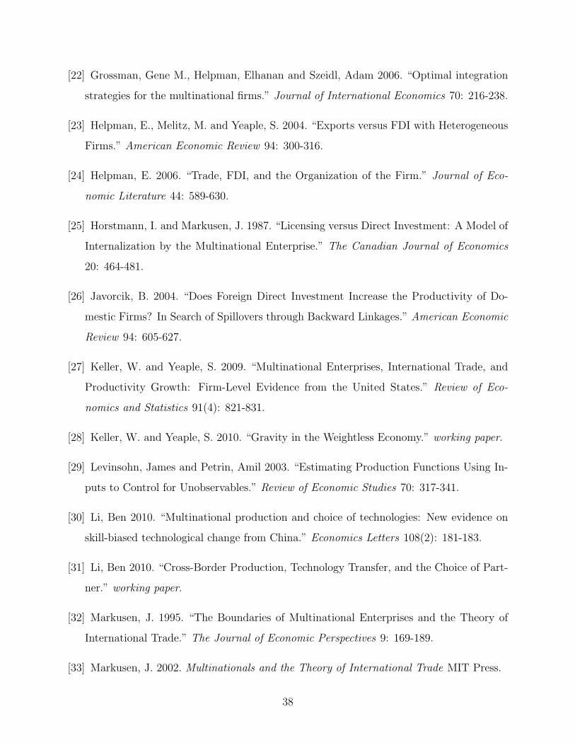
[22] Grossman, Gene M., Helpman, Elhanan and Szeidl, Adam 2006. “Optimal integration

strategies for the multinational firms.” Journal of International Economics 70: 216-238.

[23] Helpman, E., Melitz, M. and Yeaple, S. 2004. “Exports versus FDI with Heterogeneous

Firms.” American Economic Review 94: 300-316.

[24] Helpman, E. 2006. “Trade, FDI, and the Organization of the Firm.” Journal of Eco-

nomic Literature 44: 589-630.

[25] Horstmann, I. and Markusen, J. 1987. “Licensing versus Direct Investment: A Model of

Internalization by the Multinational Enterprise.” The Canadian Journal of Economics

20: 464-481.

[26] Javorcik, B. 2004. “Does Foreign Direct Investment Increase the Productivity of Do-

mestic Firms? In Search of Spillovers through Backward Linkages.” American Economic

Review 94: 605-627.

[27] Keller, W. and Yeaple, S. 2009. “Multinational Enterprises, International Trade, and

Productivity Growth: Firm-Level Evidence from the United States.” Review of Eco-

nomics and Statistics 91(4): 821-831.

[28] Keller, W. and Yeaple, S. 2010. “Gravity in the Weightless Economy.” working paper.

[29] Levinsohn, James and Petrin, Amil 2003. “Estimating Production Functions Using In-

puts to Control for Unobservables.” Review of Economic Studies 70: 317-341.

[30] Li, Ben 2010. “Multinational production and choice of technologies: New evidence on

skill-biased technological change from China.” Economics Letters 108(2): 181-183.

[31] Li, Ben 2010. “Cross-Border Production, Technology Transfer, and the Choice of Part-

ner.” working paper.

[32] Markusen, J. 1995. “The Boundaries of Multinational Enterprises and the Theory of

International Trade.” The Journal of Economic Perspectives 9: 169-189.

[33] Markusen, J. 2002. Multinationals and the Theory of International Trade MIT Press.

38

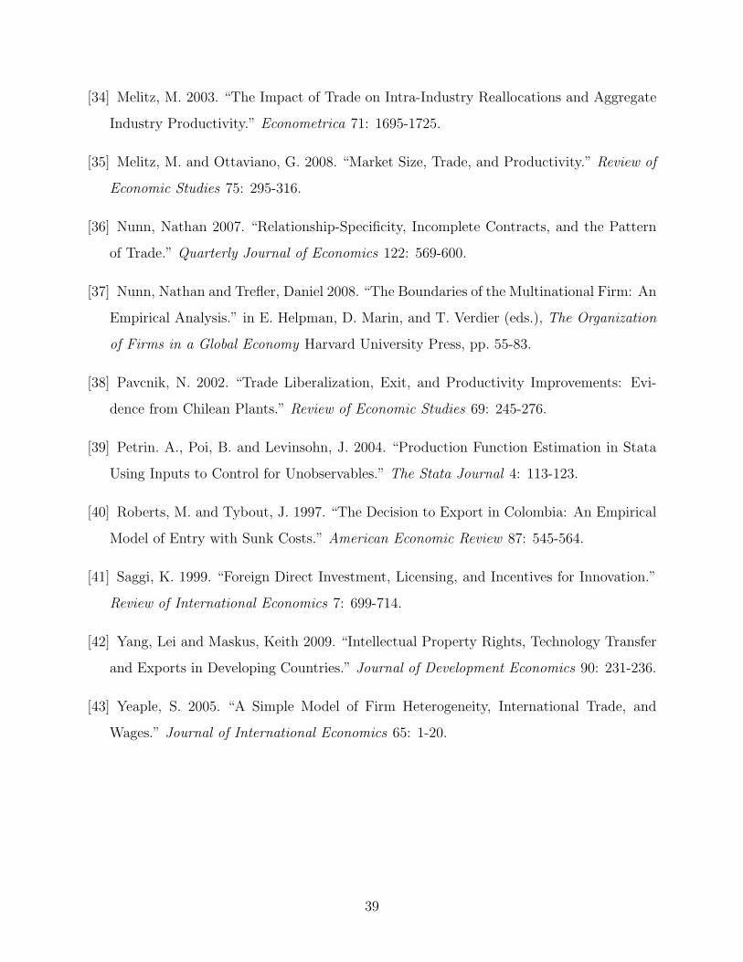
[34] Melitz, M. 2003. “The Impact of Trade on Intra-Industry Reallocations and Aggregate

Industry Productivity.” Econometrica 71: 1695-1725.

[35] Melitz, M. and Ottaviano, G. 2008. “Market Size, Trade, and Productivity.” Review of

Economic Studies 75: 295-316.

[36] Nunn, Nathan 2007. “Relationship-Specificity, Incomplete Contracts, and the Pattern

of Trade.” Quarterly Journal of Economics 122: 569-600.

[37] Nunn, Nathan and Trefler, Daniel 2008. “The Boundaries of the Multinational Firm: An

Empirical Analysis.” in E. Helpman, D. Marin, and T. Verdier (eds.), The Organization

of Firms in a Global Economy Harvard University Press, pp. 55-83.

[38] Pavcnik, N. 2002. “Trade Liberalization, Exit, and Productivity Improvements: Evi-

dence from Chilean Plants.” Review of Economic Studies 69: 245-276.

[39] Petrin. A., Poi, B. and Levinsohn, J. 2004. “Production Function Estimation in Stata

Using Inputs to Control for Unobservables.” The Stata Journal 4: 113-123.

[40] Roberts, M. and Tybout, J. 1997. “The Decision to Export in Colombia: An Empirical

Model of Entry with Sunk Costs.” American Economic Review 87: 545-564.

[41] Saggi, K. 1999. “Foreign Direct Investment, Licensing, and Incentives for Innovation.”

Review of International Economics 7: 699-714.

[42] Yang, Lei and Maskus, Keith 2009. “Intellectual Property Rights, Technology Transfer

and Exports in Developing Countries.” Journal of Development Economics 90: 231-236.

[43] Yeaple, S. 2005. “A Simple Model of Firm Heterogeneity, International Trade, and

Wages.” Journal of International Economics 65: 1-20.

39

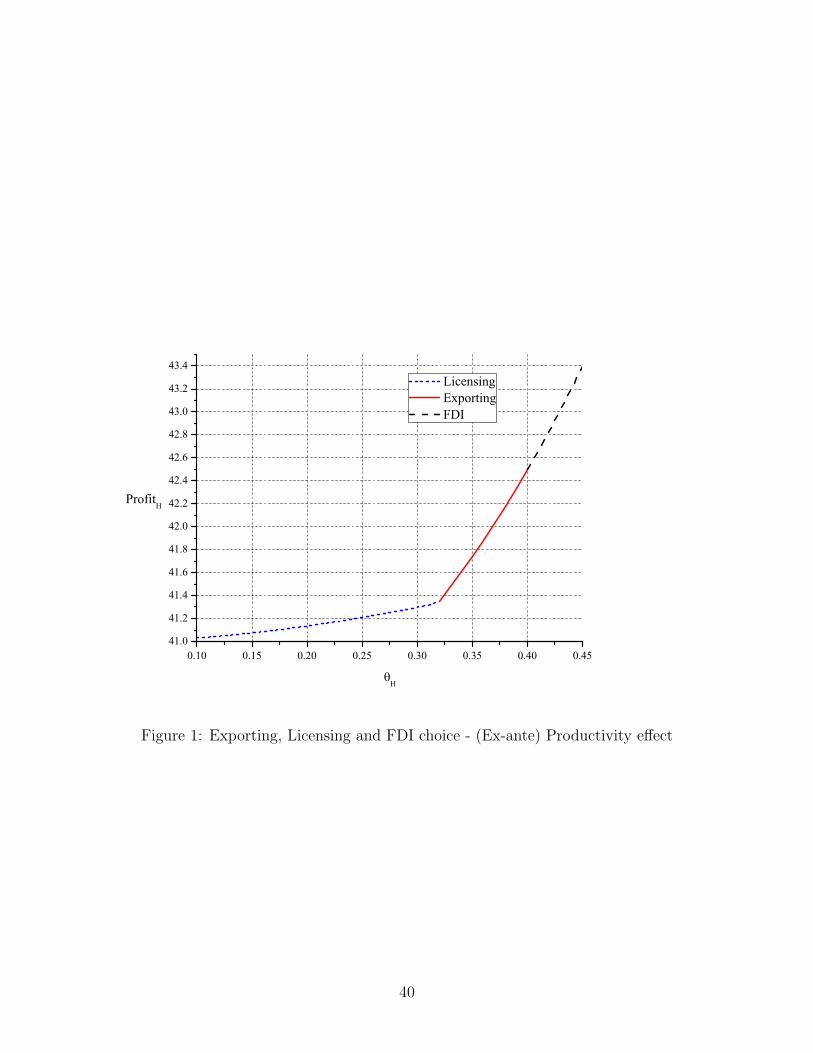
0.10 0.15 0.20 0.25 0.30 0.35 0.40 0.4541.0

41.2

41.4

41.6

41.8

42.0

42.2

42.4

42.6

42.8

43.0

43.2

43.4

ProfitH

H

Licensing Exporting FDI

Figure 1: Exporting, Licensing and FDI choice - (Ex-ante) Productivity effect

40

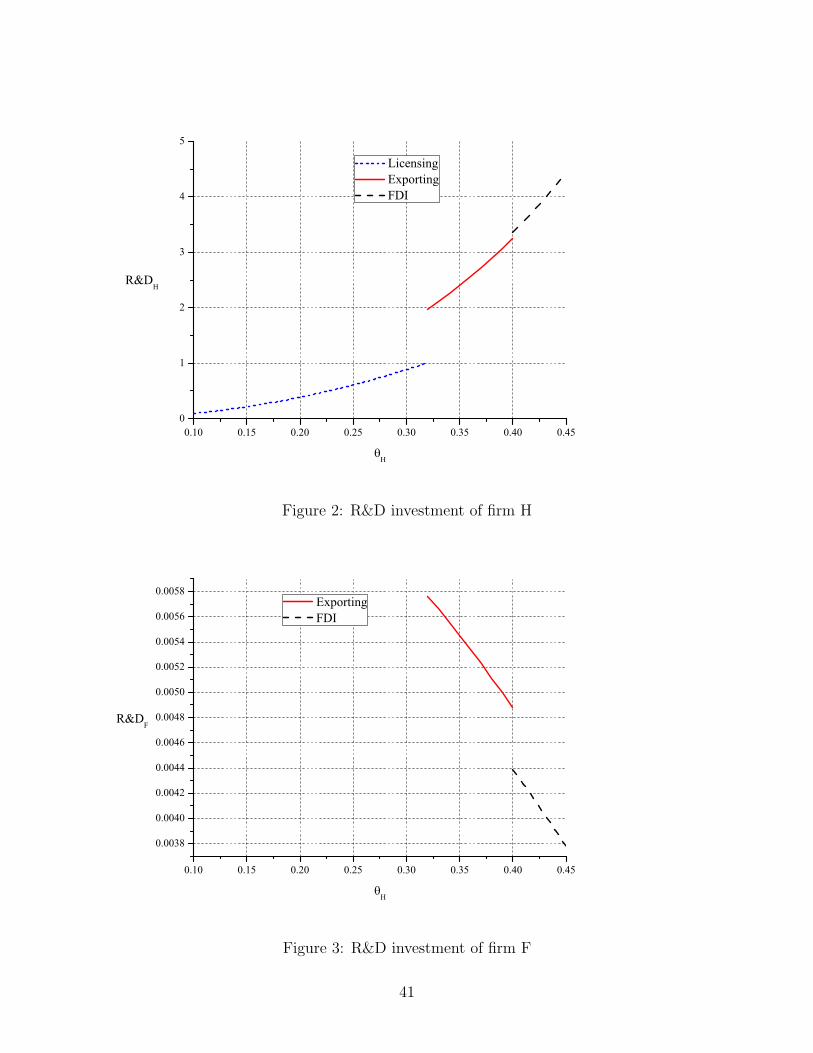
0.10 0.15 0.20 0.25 0.30 0.35 0.40 0.450

1

2

3

4

5

R&DH

H

Licensing Exporting FDI

Figure 2: R&D investment of firm H

0.10 0.15 0.20 0.25 0.30 0.35 0.40 0.45

0.0038

0.0040

0.0042

0.0044

0.0046

0.0048

0.0050

0.0052

0.0054

0.0056

0.0058

R&DF

H

Exporting FDI

Figure 3: R&D investment of firm F

41

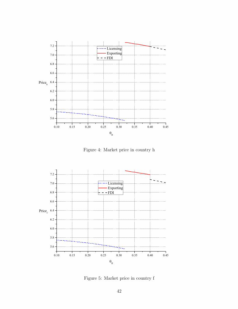
0.10 0.15 0.20 0.25 0.30 0.35 0.40 0.45

5.6

5.8

6.0

6.2

6.4

6.6

6.8

7.0

7.2

Priceh

H

Licensing Exporting FDI

Figure 4: Market price in country h

0.10 0.15 0.20 0.25 0.30 0.35 0.40 0.45

5.6

5.8

6.0

6.2

6.4

6.6

6.8

7.0

7.2

Pricef

H

Licensing Exporting FDI

Figure 5: Market price in country f

42

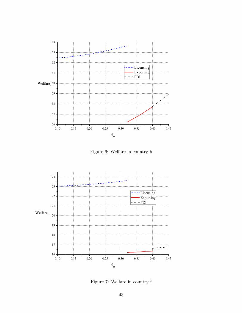
0.10 0.15 0.20 0.25 0.30 0.35 0.40 0.4556

57

58

59

60

61

62

63

64

Welfareh

H

Licensing Exporting FDI

Figure 6: Welfare in country h

0.10 0.15 0.20 0.25 0.30 0.35 0.40 0.4516

17

18

19

20

21

22

23

24

Welfaref

H

Licensing Exporting FDI

Figure 7: Welfare in country f

43

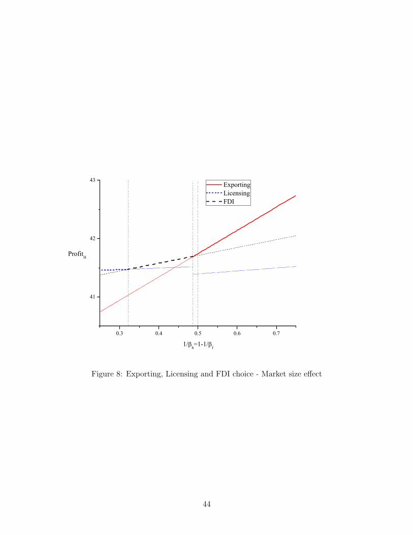
0.3 0.4 0.5 0.6 0.7

41

42

43

ProfitH

1/h=1-1/

f

Exporting Licensing FDI

Figure 8: Exporting, Licensing and FDI choice - Market size effect

44

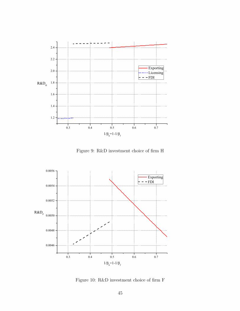
0.3 0.4 0.5 0.6 0.7

1.2

1.4

1.6

1.8

2.0

2.2

2.4

R&DH

1/h=1-1/

f

Exporting Licensing FDI

Figure 9: R&D investment choice of firm H

0.3 0.4 0.5 0.6 0.7

0.0046

0.0048

0.0050

0.0052

0.0054

0.0056

R&DF

1/h=1-1/

f

Exporting FDI

Figure 10: R&D investment choice of firm F

45

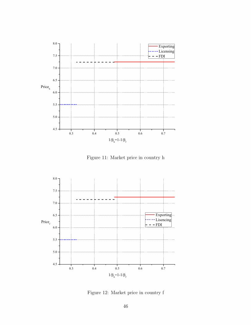
0.3 0.4 0.5 0.6 0.74.5

5.0

5.5

6.0

6.5

7.0

7.5

8.0

Priceh

1/h=1-1/

f

Exporting Licensing FDI

Figure 11: Market price in country h

0.3 0.4 0.5 0.6 0.74.5

5.0

5.5

6.0

6.5

7.0

7.5

8.0

Pricef

1/h=1-1/

f

Exporting Lisencing FDI

Figure 12: Market price in country f

46

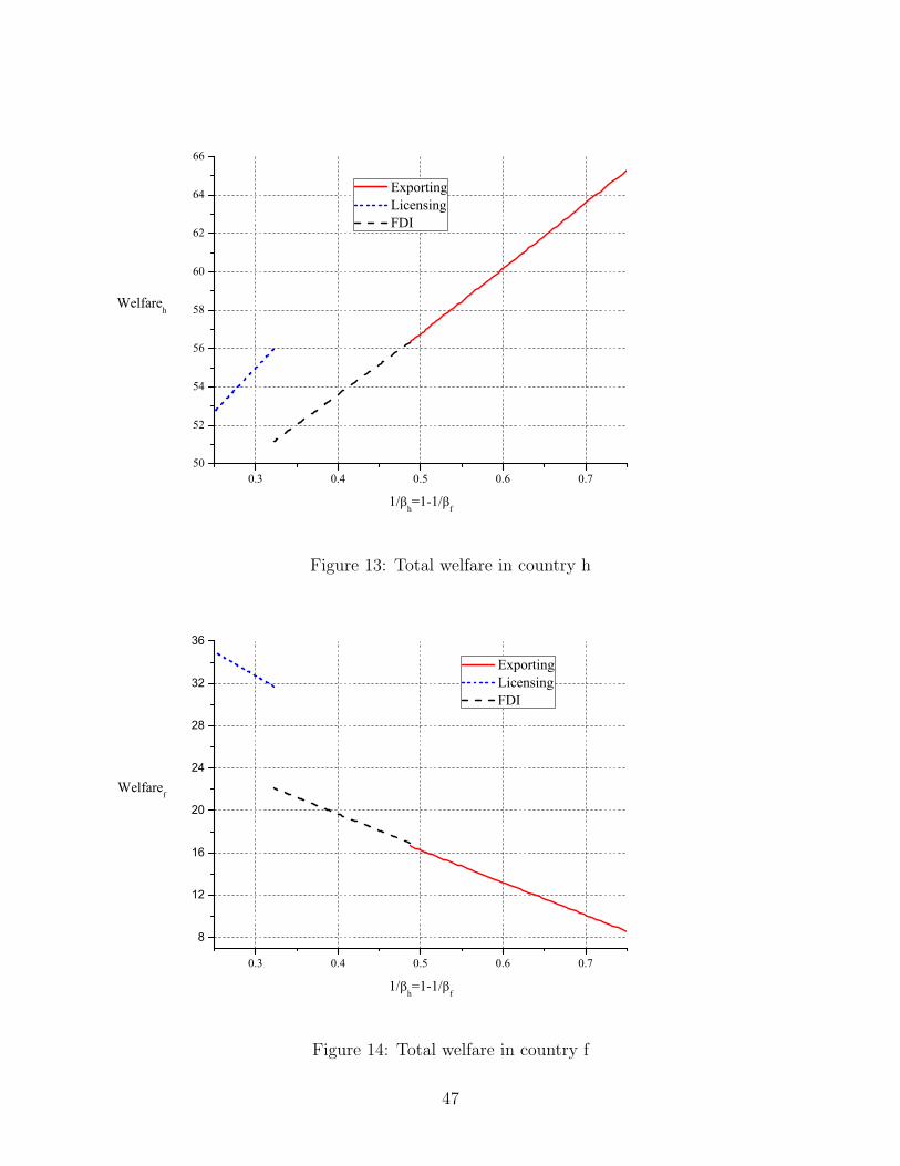
0.3 0.4 0.5 0.6 0.750

52

54

56

58

60

62

64

66

Welfareh

1/h=1-1/

f

Exporting Licensing FDI

Figure 13: Total welfare in country h

0.3 0.4 0.5 0.6 0.7

8

12

16

20

24

28

32

36

Welfaref

1/h=1-1/

f

Exporting Licensing FDI

Figure 14: Total welfare in country f

47

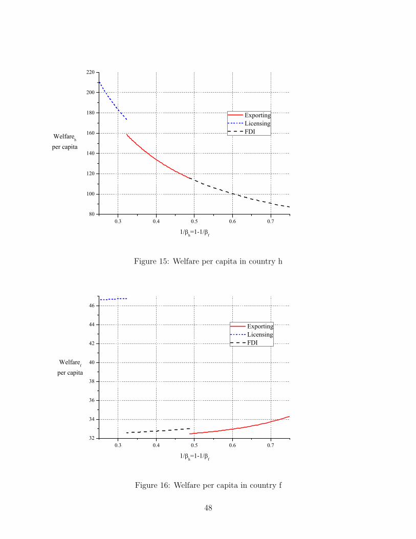
0.3 0.4 0.5 0.6 0.780

100

120

140

160

180

200

220

Welfareh

per capita

1/h=1-1/

f

Exporting Licensing FDI

Figure 15: Welfare per capita in country h

0.3 0.4 0.5 0.6 0.732

34

36

38

40

42

44

46

Welfaref

per capita

1/h=1-1/

f

Exporting Licensing FDI

Figure 16: Welfare per capita in country f

48

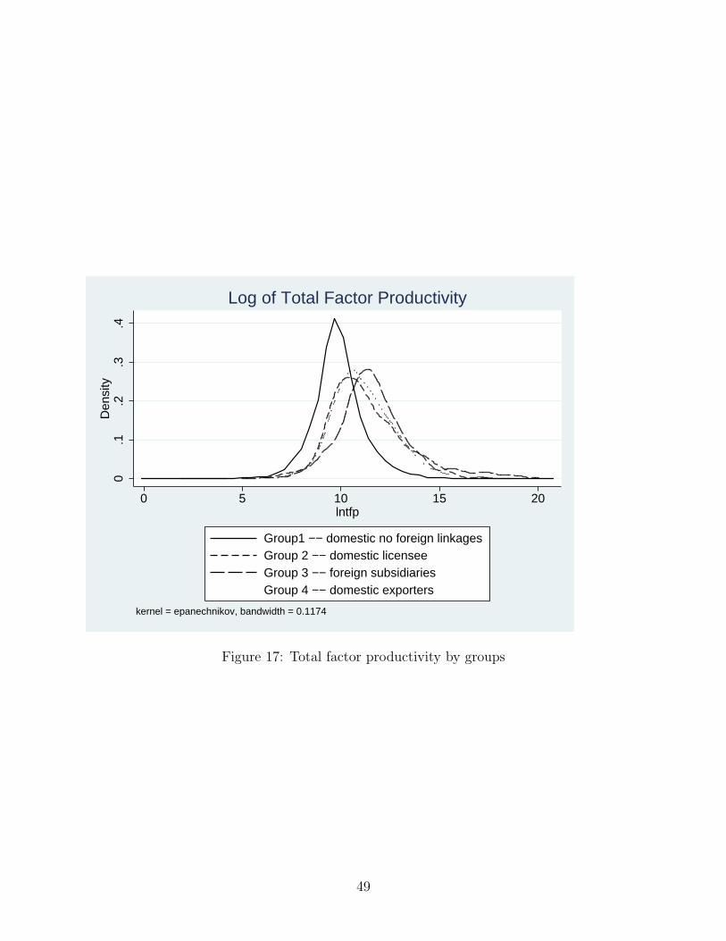
0.1

.2.3

.4D

ensi

ty

0 5 10 15 20lntfp

Group1 −− domestic no foreign linkagesGroup 2 −− domestic licenseeGroup 3 −− foreign subsidiariesGroup 4 −− domestic exporters

kernel = epanechnikov, bandwidth = 0.1174

Log of Total Factor Productivity

Figure 17: Total factor productivity by groups

49

 

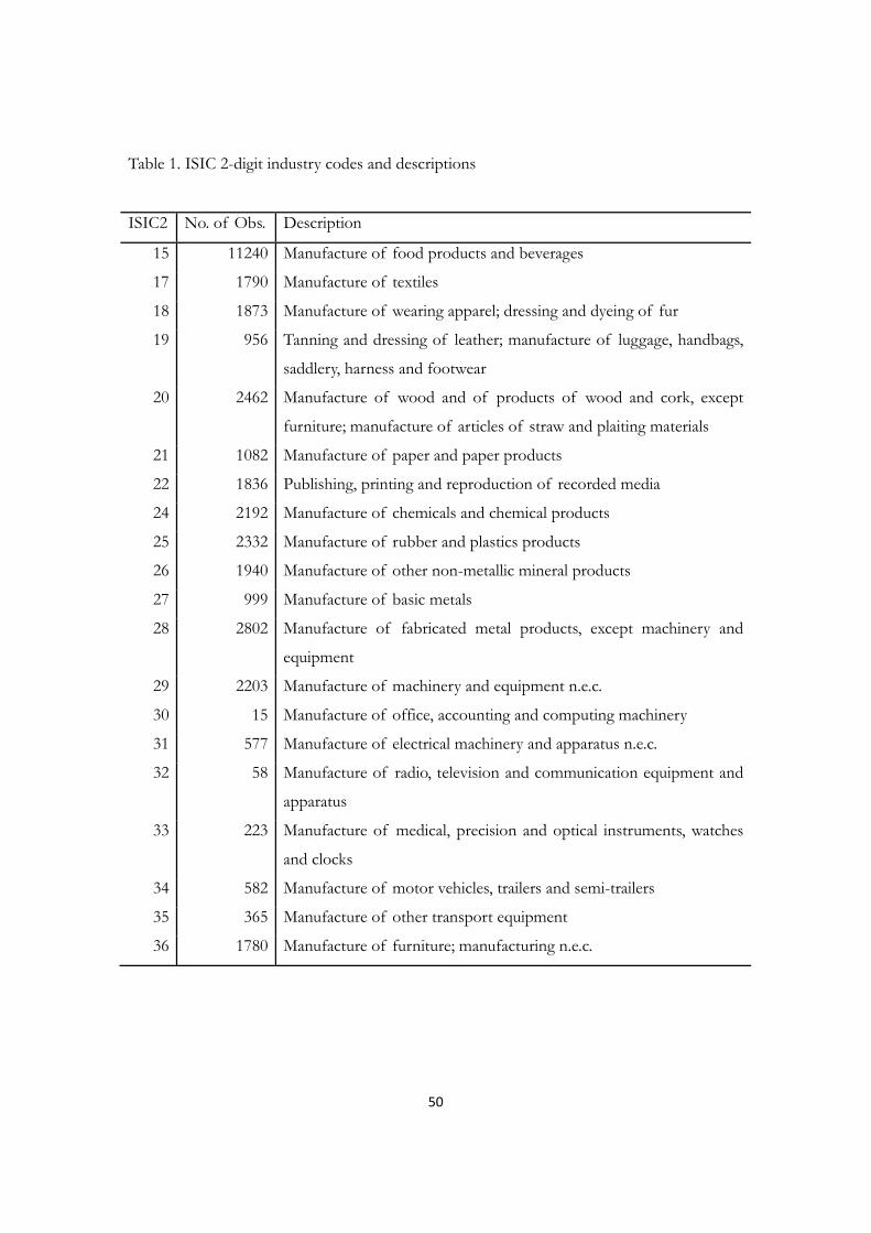
50  

Table 1. ISIC 2-digit industry codes and descriptions

ISIC2 No. of Obs. Description

15 11240 Manufacture of food products and beverages

17 1790 Manufacture of textiles

18 1873 Manufacture of wearing apparel; dressing and dyeing of fur

19 956 Tanning and dressing of leather; manufacture of luggage, handbags,

saddlery, harness and footwear

20 2462 Manufacture of wood and of products of wood and cork, except

furniture; manufacture of articles of straw and plaiting materials

21 1082 Manufacture of paper and paper products

22 1836 Publishing, printing and reproduction of recorded media

24 2192 Manufacture of chemicals and chemical products

25 2332 Manufacture of rubber and plastics products

26 1940 Manufacture of other non-metallic mineral products

27 999 Manufacture of basic metals

28 2802 Manufacture of fabricated metal products, except machinery and

equipment

29 2203 Manufacture of machinery and equipment n.e.c.

30 15 Manufacture of office, accounting and computing machinery

31 577 Manufacture of electrical machinery and apparatus n.e.c.

32 58 Manufacture of radio, television and communication equipment and

apparatus

33 223 Manufacture of medical, precision and optical instruments, watches

and clocks

34 582 Manufacture of motor vehicles, trailers and semi-trailers

35 365 Manufacture of other transport equipment

36 1780 Manufacture of furniture; manufacturing n.e.c.

   

 

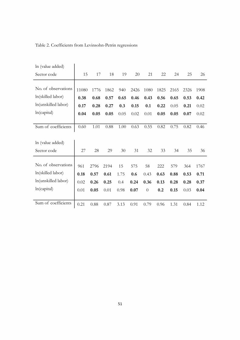
51  

Table 2. Coefficients from Levinsohn-Petrin regressions

ln (value added)

Sector code 15 17 18 19 20 21 22 24 25 26

No. of observations 11080 1776 1862 940 2426 1080 1825 2165 2326 1908ln(skilled labor) 0.38 0.68 0.57 0.65 0.46 0.43 0.56 0.65 0.53 0.42

ln(unskilled labor) 0.17 0.28 0.27 0.3 0.15 0.1 0.22 0.05 0.21 0.02ln(capital) 0.04 0.05 0.05 0.05 0.02 0.01 0.05 0.05 0.07 0.02

Sum of coefficients 0.60 1.01 0.88 1.00 0.63 0.55 0.82 0.75 0.82 0.46

ln (value added)

Sector code 27 28 29 30 31 32 33 34 35 36

No. of observations 961 2796 2194 15 575 58 222 579 364 1767ln(skilled labor) 0.18 0.57 0.61 1.75 0.6 0.43 0.63 0.88 0.53 0.71

ln(unskilled labor) 0.02 0.26 0.25 0.4 0.24 0.36 0.13 0.28 0.28 0.37

ln(capital) 0.01 0.05 0.01 0.98 0.07 0 0.2 0.15 0.03 0.04

Sum of coefficients 0.21 0.88 0.87 3.13 0.91 0.79 0.96 1.31 0.84 1.12    

 

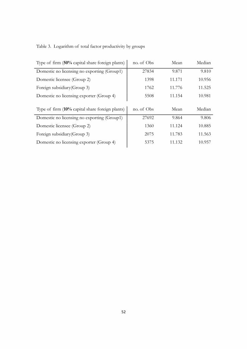
52  

Table 3. Logarithm of total factor productivity by groups

Type of firm (50% capital share foreign plants) no. of Obs Mean Median

Domestic no licensing no exporting (Group1) 27834 9.871 9.810

Domestic licensee (Group 2) 1398 11.171 10.956

Foreign subsidiary(Group 3) 1762 11.776 11.525

Domestic no licensing exporter (Group 4) 5508 11.154 10.981

 

Type of firm (10% capital share foreign plants) no. of Obs Mean Median

Domestic no licensing no exporting (Group1) 27692 9.864 9.806

Domestic licensee (Group 2) 1360 11.124 10.885

Foreign subsidiary(Group 3) 2075 11.783 11.563

Domestic no licensing exporter (Group 4) 5375 11.132 10.957

   

 

 

 

 

 

 

 

 

 

 

 

 

 

 

 

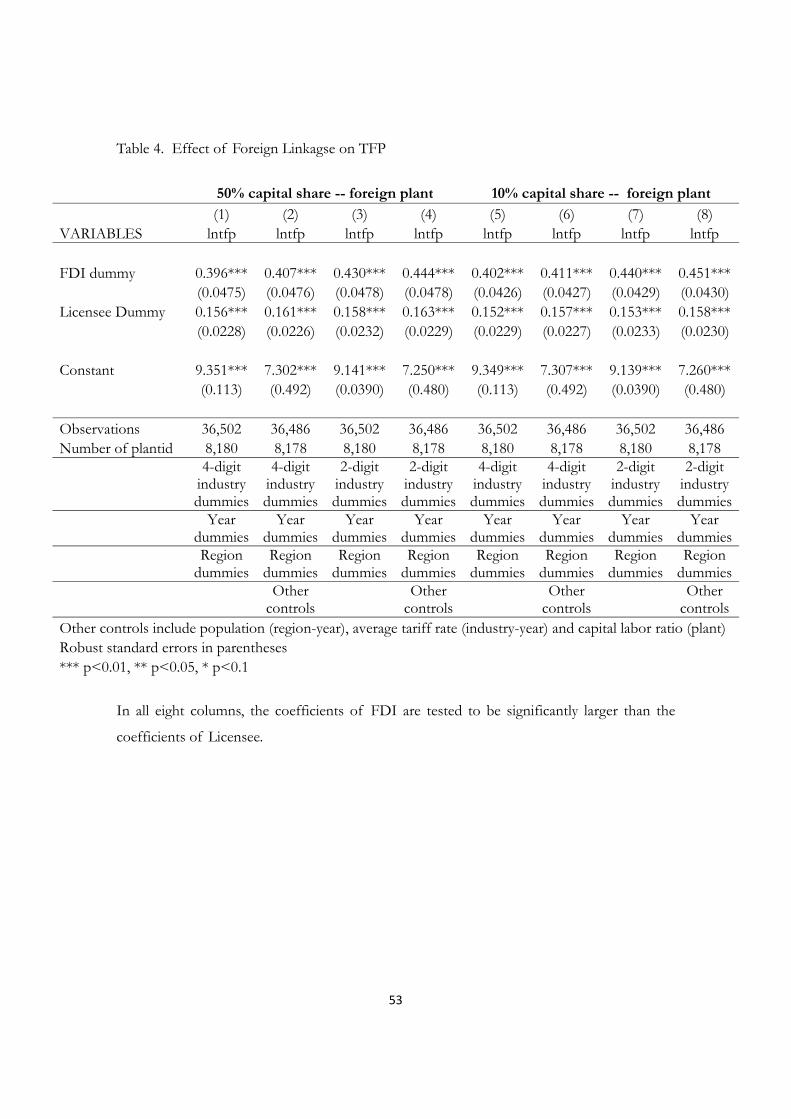
53  

Table 4. Effect of Foreign Linkagse on TFP

In all eight columns, the coefficients of FDI are tested to be significantly larger than the

coefficients of Licensee.

50% capital share -- foreign plant 10% capital share -- foreign plant (1) (2) (3) (4) (5) (6) (7) (8) VARIABLES lntfp lntfp lntfp lntfp lntfp lntfp lntfp lntfp FDI dummy 0.396*** 0.407*** 0.430*** 0.444*** 0.402*** 0.411*** 0.440*** 0.451***

(0.0475) (0.0476) (0.0478) (0.0478) (0.0426) (0.0427) (0.0429) (0.0430)Licensee Dummy 0.156*** 0.161*** 0.158*** 0.163*** 0.152*** 0.157*** 0.153*** 0.158***

(0.0228) (0.0226) (0.0232) (0.0229) (0.0229) (0.0227) (0.0233) (0.0230)

Constant 9.351*** 7.302*** 9.141*** 7.250*** 9.349*** 7.307*** 9.139*** 7.260***(0.113) (0.492) (0.0390) (0.480) (0.113) (0.492) (0.0390) (0.480)

Observations 36,502 36,486 36,502 36,486 36,502 36,486 36,502 36,486Number of plantid 8,180 8,178 8,180 8,178 8,180 8,178 8,180 8,178

4-digit industry dummies

4-digit industry dummies

2-digit industry dummies

2-digit industry dummies

4-digit industry dummies

4-digit industry dummies

2-digit industry dummies

2-digit industry dummies

Year dummies

Year dummies

Year dummies

Year dummies

Year dummies

Year dummies

Year dummies

Year dummies

Region dummies

Region dummies

Region dummies

Region dummies

Region dummies

Region dummies

Region dummies

Region dummies

Other controls

Other controls

Other controls

Other controls

Other controls include population (region-year), average tariff rate (industry-year) and capital labor ratio (plant) Robust standard errors in parentheses *** p<0.01, ** p<0.05, * p<0.1

 

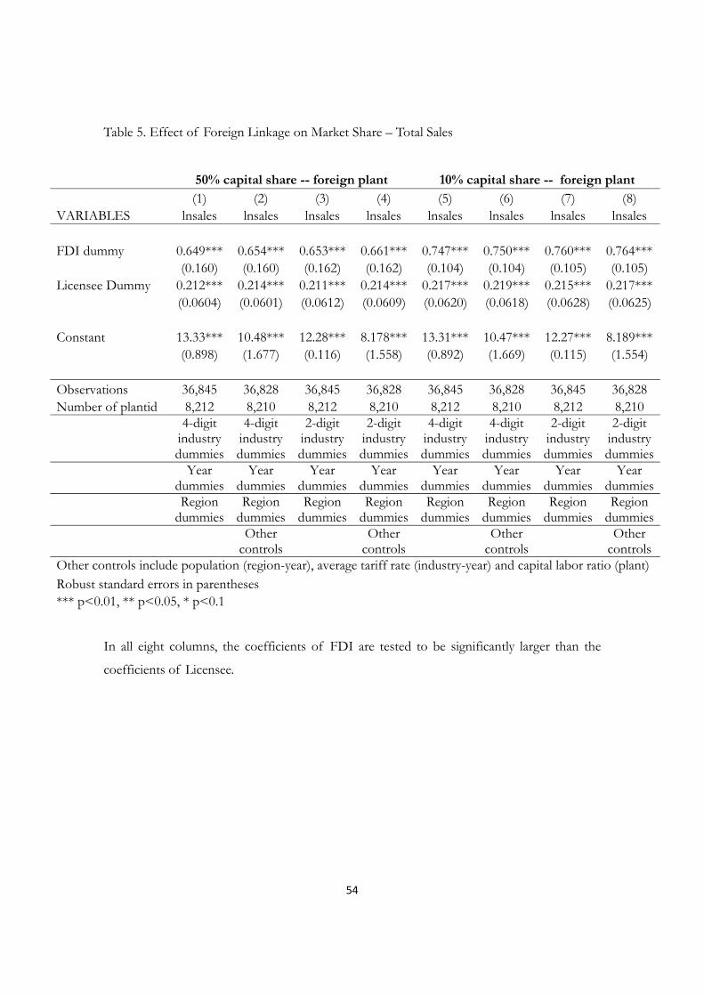
54  

Table 5. Effect of Foreign Linkage on Market Share – Total Sales

50% capital share -- foreign plant 10% capital share -- foreign plant (1) (2) (3) (4) (5) (6) (7) (8)VARIABLES lnsales lnsales lnsales lnsales lnsales lnsales lnsales lnsales FDI dummy 0.649*** 0.654*** 0.653*** 0.661*** 0.747*** 0.750*** 0.760*** 0.764***

(0.160) (0.160) (0.162) (0.162) (0.104) (0.104) (0.105) (0.105) Licensee Dummy 0.212*** 0.214*** 0.211*** 0.214*** 0.217*** 0.219*** 0.215*** 0.217***

(0.0604) (0.0601) (0.0612) (0.0609) (0.0620) (0.0618) (0.0628) (0.0625)

Constant 13.33*** 10.48*** 12.28*** 8.178*** 13.31*** 10.47*** 12.27*** 8.189***(0.898) (1.677) (0.116) (1.558) (0.892) (1.669) (0.115) (1.554)

Observations 36,845 36,828 36,845 36,828 36,845 36,828 36,845 36,828Number of plantid 8,212 8,210 8,212 8,210 8,212 8,210 8,212 8,210

4-digit industry dummies

4-digit industry dummies

2-digit industry dummies

2-digit industry dummies

4-digit industry dummies

4-digit industry dummies

2-digit industry dummies

2-digit industry dummies

Year dummies

Year dummies

Year dummies

Year dummies

Year dummies

Year dummies

Year dummies

Year dummies

Region dummies

Region dummies

Region dummies

Region dummies

Region dummies

Region dummies

Region dummies

Region dummies

Other controls

Other controls

Other controls

Other controls

Other controls include population (region-year), average tariff rate (industry-year) and capital labor ratio (plant) Robust standard errors in parentheses *** p<0.01, ** p<0.05, * p<0.1

In all eight columns, the coefficients of FDI are tested to be significantly larger than the

coefficients of Licensee.

 

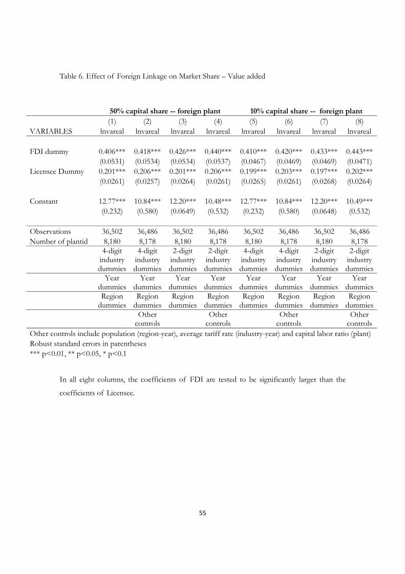
55  

Table 6. Effect of Foreign Linkage on Market Share – Value added

50% capital share -- foreign plant 10% capital share -- foreign plant (1) (2) (3) (4) (5) (6) (7) (8) VARIABLES lnvareal lnvareal lnvareal lnvareal lnvareal lnvareal lnvareal lnvareal FDI dummy 0.406*** 0.418*** 0.426*** 0.440*** 0.410*** 0.420*** 0.433*** 0.443***

(0.0531) (0.0534) (0.0534) (0.0537) (0.0467) (0.0469) (0.0469) (0.0471)Licensee Dummy 0.201*** 0.206*** 0.201*** 0.206*** 0.199*** 0.203*** 0.197*** 0.202***

(0.0261) (0.0257) (0.0264) (0.0261) (0.0265) (0.0261) (0.0268) (0.0264)

Constant 12.77*** 10.84*** 12.20*** 10.48*** 12.77*** 10.84*** 12.20*** 10.49***(0.232) (0.580) (0.0649) (0.532) (0.232) (0.580) (0.0648) (0.532)

Observations 36,502 36,486 36,502 36,486 36,502 36,486 36,502 36,486 Number of plantid 8,180 8,178 8,180 8,178 8,180 8,178 8,180 8,178

4-digit industry dummies

4-digit industry dummies

2-digit industry dummies

2-digit industry dummies

4-digit industry dummies

4-digit industry dummies

2-digit industry dummies

2-digit industry dummies

Year dummies

Year dummies

Year dummies

Year dummies

Year dummies

Year dummies

Year dummies

Year dummies

Region dummies

Region dummies

Region dummies

Region dummies

Region dummies

Region dummies

Region dummies

Region dummies

Other controls

Other controls

Other controls

Other controls

Other controls include population (region-year), average tariff rate (industry-year) and capital labor ratio (plant) Robust standard errors in parentheses *** p<0.01, ** p<0.05, * p<0.1

In all eight columns, the coefficients of FDI are tested to be significantly larger than the

coefficients of Licensee.

 

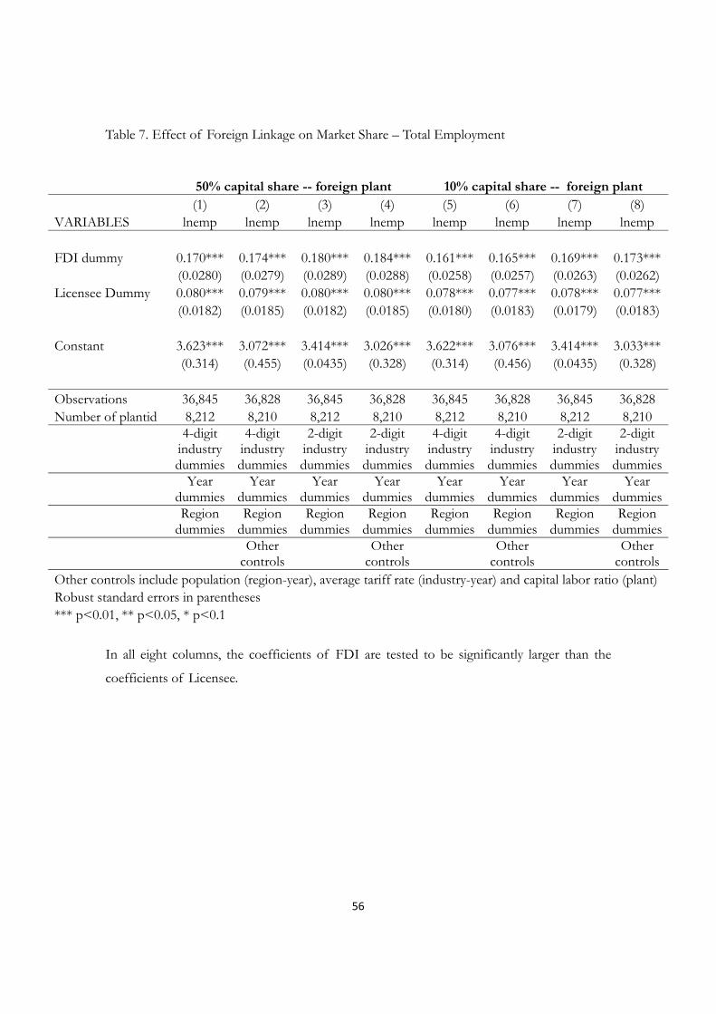
56  

Table 7. Effect of Foreign Linkage on Market Share – Total Employment

In all eight columns, the coefficients of FDI are tested to be significantly larger than the

coefficients of Licensee.

50% capital share -- foreign plant 10% capital share -- foreign plant (1) (2) (3) (4) (5) (6) (7) (8)VARIABLES lnemp lnemp lnemp lnemp lnemp lnemp lnemp lnemp FDI dummy 0.170*** 0.174*** 0.180*** 0.184*** 0.161*** 0.165*** 0.169*** 0.173***

(0.0280) (0.0279) (0.0289) (0.0288) (0.0258) (0.0257) (0.0263) (0.0262)Licensee Dummy 0.080*** 0.079*** 0.080*** 0.080*** 0.078*** 0.077*** 0.078*** 0.077***

(0.0182) (0.0185) (0.0182) (0.0185) (0.0180) (0.0183) (0.0179) (0.0183)

Constant 3.623*** 3.072*** 3.414*** 3.026*** 3.622*** 3.076*** 3.414*** 3.033***(0.314) (0.455) (0.0435) (0.328) (0.314) (0.456) (0.0435) (0.328)

Observations 36,845 36,828 36,845 36,828 36,845 36,828 36,845 36,828Number of plantid 8,212 8,210 8,212 8,210 8,212 8,210 8,212 8,210

4-digit industry dummies

4-digit industry dummies

2-digit industry dummies

2-digit industry dummies

4-digit industry dummies

4-digit industry dummies

2-digit industry dummies

2-digit industry dummies

Year dummies

Year dummies

Year dummies

Year dummies

Year dummies

Year dummies

Year dummies

Year dummies

Region dummies

Region dummies

Region dummies

Region dummies

Region dummies

Region dummies

Region dummies

Region dummies

Other controls

Other controls

Other controls

Other controls

Other controls include population (region-year), average tariff rate (industry-year) and capital labor ratio (plant) Robust standard errors in parentheses *** p<0.01, ** p<0.05, * p<0.1

 

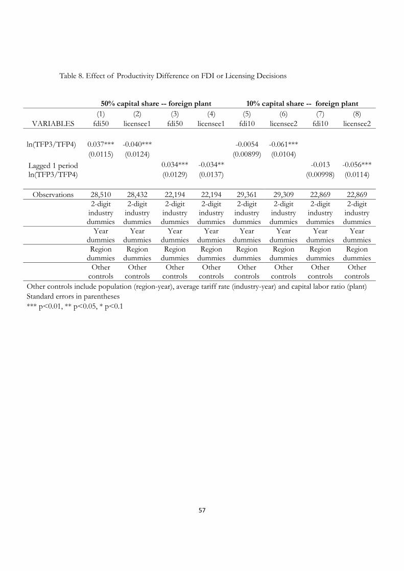
57  

Table 8. Effect of Productivity Difference on FDI or Licensing Decisions

50% capital share -- foreign plant 10% capital share -- foreign plant (1) (2) (3) (4) (5) (6) (7) (8)

VARIABLES fdi50 licensee1 fdi50 licensee1 fdi10 licensee2 fdi10 licensee2

ln(TFP3/TFP4) 0.037*** -0.040*** -0.0054 -0.061*** (0.0115) (0.0124) (0.00899) (0.0104)

Lagged 1 period ln(TFP3/TFP4)

0.034*** -0.034** -0.013 -0.056***(0.0129) (0.0137) (0.00998) (0.0114)

Observations 28,510 28,432 22,194 22,194 29,361 29,309 22,869 22,8692-digit

industry dummies

2-digit industry dummies

2-digit industry dummies

2-digit industry dummies

2-digit industry dummies

2-digit industry dummies

2-digit industry dummies

2-digit industry dummies

Year dummies

Year dummies

Year dummies

Year dummies

Year dummies

Year dummies

Year dummies

Year dummies

Region dummies

Region dummies

Region dummies

Region dummies

Region dummies

Region dummies

Region dummies

Region dummies

Other controls

Other controls

Other controls

Other controls

Other controls

Other controls

Other controls

Other controls

Other controls include population (region-year), average tariff rate (industry-year) and capital labor ratio (plant) Standard errors in parentheses *** p<0.01, ** p<0.05, * p<0.1

 

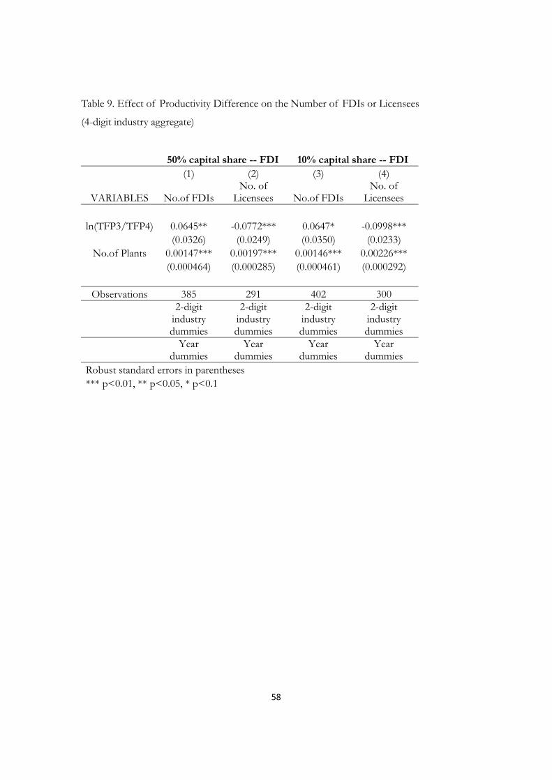
58  

Table 9. Effect of Productivity Difference on the Number of FDIs or Licensees

(4-digit industry aggregate)

50% capital share -- FDI 10% capital share -- FDI (1) (2) (3) (4)

VARIABLES No.of FDIs No. of

Licensees No.of FDIsNo. of

Licensees

ln(TFP3/TFP4) 0.0645** -0.0772*** 0.0647* -0.0998*** (0.0326) (0.0249) (0.0350) (0.0233)

No.of Plants 0.00147*** 0.00197*** 0.00146*** 0.00226*** (0.000464) (0.000285) (0.000461) (0.000292)

Observations 385 291 402 300 2-digit

industry dummies

2-digit industry dummies

2-digit industry dummies

2-digit industry dummies

Year dummies

Year dummies

Year dummies

Year dummies

Robust standard errors in parentheses*** p<0.01, ** p<0.05, * p<0.1

 

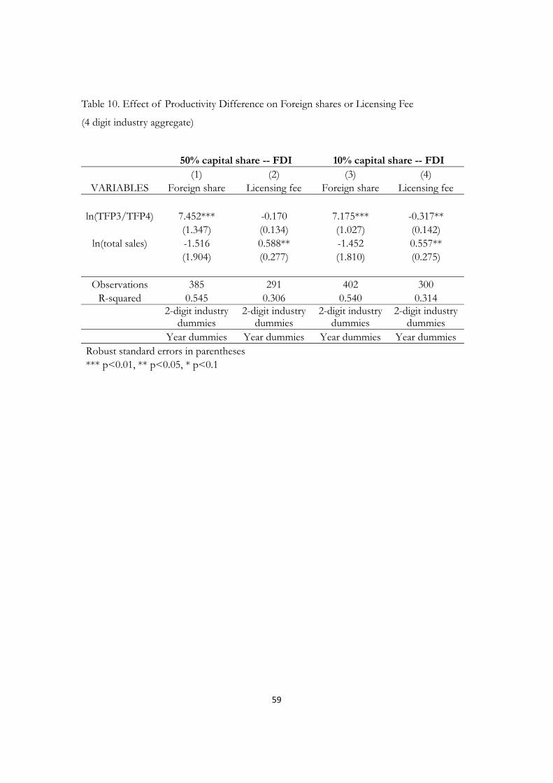
59  

Table 10. Effect of Productivity Difference on Foreign shares or Licensing Fee

(4 digit industry aggregate)

50% capital share -- FDI 10% capital share -- FDI (1) (2) (3) (4)

VARIABLES Foreign share Licensing fee Foreign share Licensing fee

ln(TFP3/TFP4) 7.452*** -0.170 7.175*** -0.317** (1.347) (0.134) (1.027) (0.142)

ln(total sales) -1.516 0.588** -1.452 0.557** (1.904) (0.277) (1.810) (0.275)

Observations 385 291 402 300 R-squared 0.545 0.306 0.540 0.314

2-digit industry dummies

2-digit industry dummies

2-digit industry dummies

2-digit industry dummies

Year dummies Year dummies Year dummies Year dummies Robust standard errors in parentheses *** p<0.01, ** p<0.05, * p<0.1