Embed Size (px)
Citation preview
EXPORTS AND ECONOMIC GROWTH:
AN EMPIRICAL INVESTIGATION OF E.U,
U.S.A AND JAPAN USING CAUSALITY TESTS
Nikolaos Dritsakis
Department of Applied Informatics
University of Macedonia
Economics and Social Sciences
156 Egnatia Street
P.O box 1591
540 06 Thessaloniki, Greece
FAX: (2310) 891290
e-mail: [email protected]

2
EXPORTS AND ECONOMIC GROWTH:
AN EMPIRICAL INVESTIGATION OF E.U,
U.S.A AND JAPAN USING CAUSALITY TESTS
Abstract
This paper investigates the relationship between exports and economic growth in the
three of the largest exporting countries in the world, such as European Union, United
States of America and Japan. For this purpose we have used Granger causality
analysis based on error correction model. The results of this paper suggested that
exports have a causal effect on the development process for the countries of European
Union, USA, while there is no causal relationship between the examined variables for
Japan.
keywords: exports, economic growth, cointegration, Granger causality
JEL. O10, C22
3
1. Introduction There is a wide body of literature analyzing the theoretical links between exports
and economic growth. According to this literature, the relationship between exports
and economic growth is determined by different factors. Clearly, since exports are a
component of GDP, exports growth contributes directly to GDP growth. Exports
relax binding foreign exchange constraints and allow increases in imported capital
goods and intermediate goods (McKinnon 1964, Chenery and Strout 1966). Also
exports allow poor countries with narrow domestic markets to benefit from
economies of scale (Helpman and Krugman 1985). In addition, exports lead to
improved efficiency in resource allocation and, in particular, improved capital
utilization owing to competition in world markets (Balassa 1978, Bhagwati and
Srinivasan 1979, Krueger 1980).
The ratio of exports to gross domestic product also provides us information about
the importance of exports in the national economy. Since the ratio of exports to
gross domestic product is an index of openness, a larger ratio of exports to gross
domestic product indicates a more open economy. Larger economies – as measured
by area, population, and size of the domestic market- can produce and absorb a
larger share of their output domestically, they tend to have lower ratios (Pereira and
Xu 2000).
On the other hand low ratios of exports to gross domestic product can reflect
restrictive trade policies. Nevertheless, the low-ratio countries, which are classified
as potentially oriented by the World Bank, are fitted to this category appropriately.
Four different views can be distinguished for the relationship between exports and
economic growth. The first is the neoclassical export-led growth hypothesis. This
4
theory suggests that the direction of causation is running from exports to economic
growth for the following reasons:
• Export expansion will increase productivity by offering greater economies of
scale (Helpman and Krugman 1985).
• Export expansion brings about higher-quality products because of the exporter’s
exposure to international consumption patterns (Krueger 1985).
• Exports will lead a firm to overinvest in a new technology as a strategy for a
precommitment to a larger scale of output, increasing the rate of capital
formation and technological change (Rodrik 1988, Ghirmay, Grabowski and
Sharma 2001).
• An export-oriented approach in a labor-surplus economy permits the rapid
expansion of employment and real wages (Krueger 1985, Abdulai and Jaquet
2002).
• Exports contribute to a relaxation of foreign exchange constraints (Voivodas
1973, Afxentiou and Serletis, 1992).
The second view is that causality runs from economic growth to exports. Higher
productivity leads to a lower unit cost, which facilitates exports growth (Kaldor
1967). Economic growth affect exports growth if the domestic production increases
faster than the domestic demand (Sharma and Dhakal 1994), Ahmad and Harnhirun
1996, Shan and Tian 1998).
The third view, which is a combination of the first and the second views, suggests
that there can be a bilateral causal relationship between exports and economic
growth (Ghartey 1993, Wernerheim 2000, Ramos 2001, Hatemi-J. 2002).
5
Final, the fourth view is that there is no causal relation between exports and
economic growth, namely exports and economic growth are both the result of the
development process and technological change (Yaghmaian 1994).
For the causal analysis between exports and economic growth, recent empirical
studies have adopted the causality approach suggested by (Granger 1969 and Sims
1972). The results from causality tests are however mixed. Some studies find a
positive relationship between exports and economic growth (Sharma 1991, Xu
1996, Liu, Burridge and Sinclair 2002), while other results from causality tests are
largely negative (Βahmani-Oskooee et al 1991 and Dodaro 1993), even for those
economies such as Hong Kong, Korea, Taiwan, whose growth experience is widely
believed to result from their successful export-promoting policies.
Ιn this paper, the methodology proposed by (Granger 1969 and Sims 1972) for the
causality tests on the relationship between exports and economic growth is applied.
This methodology is based on the estimation of bivariate relationships between the
two variables. These tests are designed to capture exclusively the short-run dynamics
between the two variables. However, there might exist a long-run relationship
between these variables. For this reason the cointegration analysis is used to test the
long-run equilibrium relationship between exports and economic growth for the
examined countries. (Dritsakis and Adamopoulos 2004)
The aim of this paper is to investigate the relationship between exports and
economic growth for these three economies, which are mainly the major exporters
in the world market. The remainder of the paper proceeds as follows: Section 2
describes the theoretical framework of this paper. Section 3 presents the results of
unit root tests, while the cointegration analysis between the used variables is implied
6
in Section 4. The causality analysis based on error correction model is deployed in
Section 5. Finally, section 6 provides the conclusions of this paper.
2. The theoretical framework
In order to examine the relationship between exports and economic growth, the
present paper uses two models from the existing literature (Feder 1982, Ram 1985,
1987). One is a production function-type framework in which the level of exports,
the level of government expenditures and the terms of trade enter as ‘inputs’ in the
production process (Khalifa-Al Yousif 1997, Dritsakis and Vazakidis 2003). The
open nature of the three countries explains the inclusion of both terms of trade, the
level of exports, the labour, the capital and the level of government expenditures as
possible explanatory variables in the production function. This specification can be
derived from the following general aggregate production function
Y = f ( L, K, X, G, T ) (1)
where:
Υ = Real aggregate output
L = Labour
K = Capital
X = Exports
G = Government spending
T = Terms of trade
7
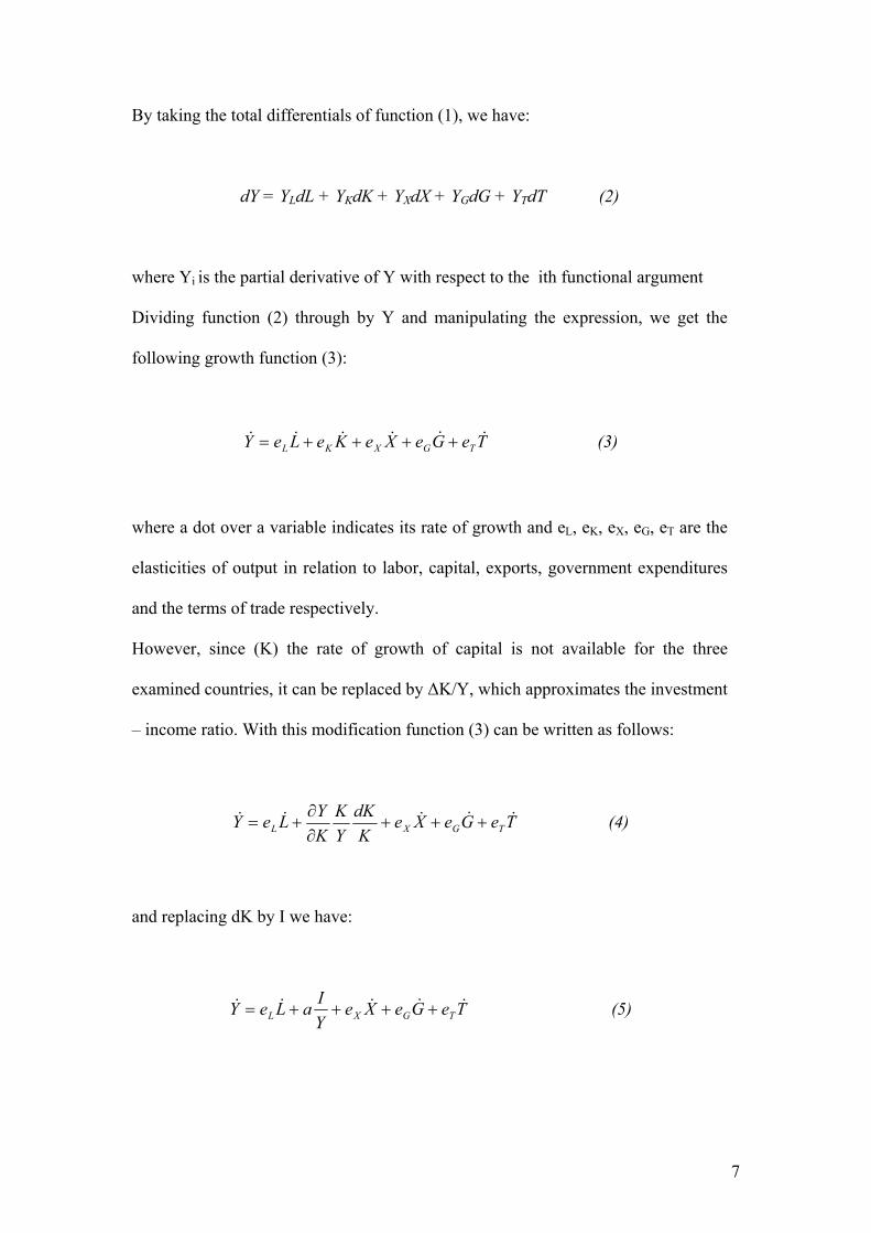
By taking the total differentials of function (1), we have:
dY = YLdL + YKdK + YXdX + YGdG + YTdT (2)
where Υi is the partial derivative of Υ with respect to the ith functional argument
Dividing function (2) through by Y and manipulating the expression, we get the
following growth function (3):
TeGeXeKeLeY TGXKL&&&&&& ++++= (3)
where a dot over a variable indicates its rate of growth and eL, eK, eX, eG, eT are the
elasticities of output in relation to labor, capital, exports, government expenditures
and the terms of trade respectively.
However, since (K) the rate of growth of capital is not available for the three
examined countries, it can be replaced by ΔΚ/Υ, which approximates the investment
– income ratio. With this modification function (3) can be written as follows:
TeGeXeK
dKYK
KYLeY TGXL
&&&&& +++∂∂
+= (4)
and replacing dK by Ι we have:
TeGeXeYIaLeY TGXL
&&&&& ++++= (5)
8
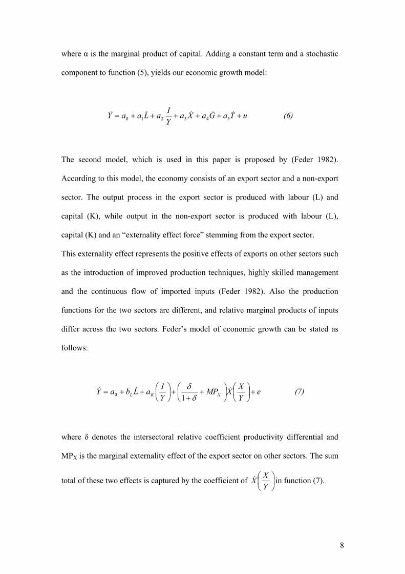
where α is the marginal product of capital. Adding a constant term and a stochastic
component to function (5), yields our economic growth model:
uTaGaXaYIaLaaY ++++++= &&&&&
543210 (6)
The second model, which is used in this paper is proposed by (Feder 1982).
According to this model, the economy consists of an export sector and a non-export
sector. The output process in the export sector is produced with labour (L) and
capital (Κ), while output in the non-export sector is produced with labour (L),
capital (Κ) and an “externality effect force” stemming from the export sector.
This externality effect represents the positive effects of exports on other sectors such
as the introduction of improved production techniques, highly skilled management
and the continuous flow of imported inputs (Feder 1982). Also the production
functions for the two sectors are different, and relative marginal products of inputs
differ across the two sectors. Feder’s model of economic growth can be stated as
follows:
eYXXMP
YIaLbaY XKL +⎟
⎠⎞
⎜⎝⎛
⎟⎠⎞
⎜⎝⎛ ++
+⎟⎠⎞
⎜⎝⎛++= &&&
δδ
10 (7)
where δ denotes the intersectoral relative coefficient productivity differential and
MPX is the marginal externality effect of the export sector on other sectors. The sum
total of these two effects is captured by the coefficient of ⎟⎠⎞
⎜⎝⎛
YXX& in function (7).

9
Functions (6) and (7) will constitute the basis for the estimates reported for each of
the three examined countries. However when the coefficients of government
expenditures or the terms of trade or both in function (7) are found to be either
statistical insignificant then they are omitted.
3. Unit root tests
Many macroeconomic time series contain unit roots dominated by stochastic trends as
developed by (Nelson and Plosser 1982). Unit roots are important in examining the
stationarity of a time series because a non-stationary regressor invalidates many
standard empirical results. The presence of a stochastic trend is determined by testing
the presence of unit roots in time series data. In this study unit root test is tested using
Augmented Dickey-Fuller (ADF) (1979), and Kwiatkowski et al. (1992).
3.1 Augmented Dickey-Fuller (ADF) test
The augmented Dickey-Fuller (ADF) (1979) test is referred to the t-statistic of δ2
coefficient οn the following regression:
ΔXt = δ0 + δ1 t + δ2 Xt-1 + ∑=
− +ΔΧk
ititi u
1α (8)
The ADF regression tests for the existence of unit root of Χt, in all model variables
at time t. The variable ΔΧt-i expresses the first differences with k lags and final ut is
the variable that adjusts the errors of autocorrelation. The coefficients δ0, δ1, δ2, and

10
αi are being estimated. The null and the alternative hypothesis for the existence of
unit root in variable Xt is:
Ηο : δ2 = 0 Ηε : δ2 < 0
Τhis paper follows the suggestion of (Engle and Yoo 1987) using the Akaike
information criterion (AIC) (1974), to determine the optimal specification of Equation
(8). The appropriate order of the model is determined by computing Equation (8) over
a selected grid of values of the number of lags k and by finding the value of k at which
the AIC attains its minimum. The distribution of the ADF statistic is non-standard and
the critical values tabulated by (Mackinnon 1991) are used.
3.2 Kwiatkowski, Phillips, Schmidt, and Shin’s (KPSS) test
Since the null hypothesis in Augmented Dickey-Fuller test is that a time series
contains a unit root, this hypothesis is accepted unless there is a strong evidence
against it. However, this approach may have low power against stationary near unit
root processes. In contrast Kwiatkowski el al (1992) present a test where the null
hypothesis is that a series is stationary. The KPSS test complements the Augmented
Dickey-Fuller test in that concerns regarding the power of either test can be addressed
by comparing the significance of statistics from both tests. A stationary series has
significant Augmented Dickey-Fuller statistics and insignificant KPSS1 statistics.
1 According to Kwiatkowski et al (1992), the test of ΚPSS assumes that a time series can be composed into three components, a deterministic time trend, a random walk and a stationary error:
yt = δt + rt + εt
where rt is a random walk rt = rt-1 + ut.. The ut is iid (0, 2uσ ).
11
INSERT TABLE 1
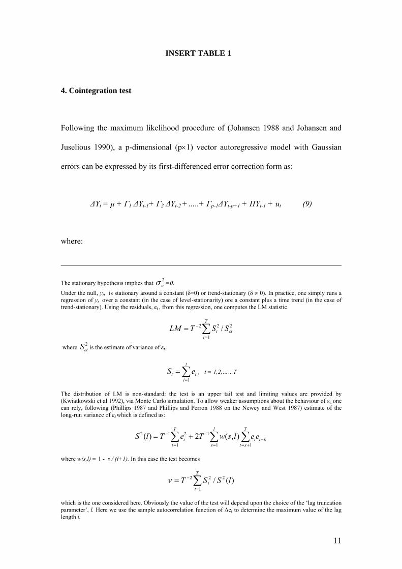
4. Cointegration test
Following the maximum likelihood procedure of (Johansen 1988 and Johansen and
Juselious 1990), a p-dimensional (p×1) vector autoregressive model with Gaussian
errors can be expressed by its first-differenced error correction form as:
ΔΥt = μ + Γ1 ΔΥt-1+ Γ2 ΔΥt-2 +…..+ Γp-1ΔΥt-p+1 + ΠΥt-1 + ut (9)
where:
The stationary hypothesis implies that 2uσ =0.
Under the null, yt, is stationary around a constant (δ=0) or trend-stationary (δ ≠ 0). In practice, one simply runs a regression of yt over a constant (in the case of level-stationarity) ore a constant plus a time trend (in the case of trend-stationary). Using the residuals, ei , from this regression, one computes the LM statistic
∑=
−=T
ttt SSTLM
1
222 / ε
where 2tSε is the estimate of variance of εt.
∑=
=t
iit eS
1, t = 1,2,……T
The distribution of LM is non-standard: the test is an upper tail test and limiting values are provided by (Kwiatkowski et al 1992), via Monte Carlo simulation. To allow weaker assumptions about the behaviour of εt, one can rely, following (Phillips 1987 and Phillips and Perron 1988 on the Newey and West 1987) estimate of the long-run variance of εt which is defined as:
∑ ∑ ∑= = +=
−−− +=
T
t
l
s
T
stkiii eelswTeTlS
1 1 1
1212 ),(2)(
where w(s,l) = 1 - s / (l+1). In this case the test becomes
∑=
−=T
tt lSST
1
222 )(/ν
which is the one considered here. Obviously the value of the test will depend upon the choice of the ‘lag truncation parameter’, l. Here we use the sample autocorrelation function of Δet to determine the maximum value of the lag length l.
12
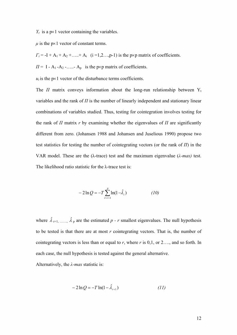
Υt is a p×1 vector containing the variables.
μ is the p×1 vector of constant terms.
Γi = -I + A1 + A2 +…..+ Ai (i =1,2…,p-1) is the p×p matrix of coefficients.
Π = I - A1 -A2 -…..- Ap is the p×p matrix of coefficients.
ut is the p×1 vector of the disturbance terms coefficients.
The Π matrix conveys information about the long-run relationship between Yt
variables and the rank of Π is the number of linearly independent and stationary linear
combinations of variables studied. Thus, testing for cointegration involves testing for
the rank of Π matrix r by examining whether the eigenvalues of Π are significantly
different from zero. (Johansen 1988 and Johansen and Juselious 1990) propose two
test statistics for testing the number of cointegrating vectors (or the rank of Π) in the
VAR model. These are the (λ-trace) test and the maximum eigenvalue (λ-max) test.
The likelihood ratio statistic for the λ-trace test is:
)ˆ1ln(ln21
i
p
riTQ λ∑
+=
−−=− (10)
where λ̂ r+1, ……., λ̂ p are the estimated p - r smallest eigenvalues. The null hypothesis
to be tested is that there are at most r cointegrating vectors. That is, the number of
cointegrating vectors is less than or equal to r, where r is 0,1, or 2…., and so forth. In
each case, the null hypothesis is tested against the general alternative.
Alternatively, the λ-max statistic is:
)ˆ1ln(ln2 1+−−=− rTQ λ (11)
13
In this test, the null hypothesis of r cointegrating vectors is tested against the
alternative hypothesis of r+1 cointegrating vectors. Thus, the null hypothesis r = 0 is
tested against the alternative that r = 1, r = 1 against the alternative r = 2, and so
forth. It is well known the cointegration tests are very sensitive to the choice of lag
length. The Schwarz Criterion (SC) (1978) and the likelihood ratio test are used to
select the number of lags required in the cointegration test.
4.1 Long-run relationships
The presence of cointegrating vectors is tested for the long-run relationships among
the set of variables considered here. The λ-trace and λ-max test statistics are
reported in Table 2 along with the number of cointegrating vectors. Using the 5%
and 10% critical values from (Johansen and Juselious 1990), it is observed that in
some cases the λ-max and λ-trace test statistics give conflicting results (USA)
(Johansen 1991) argues that such conflicting results arise from the low power of the
test in cases when the cointegration relatioship is quite close to nonstationary
boundary. It is also argued that since the trace test takes account of all (3-r) of the
smallest eigenvalues, it tends to have more power than the λ-max test. Hence, in the
conflicting cases (USA) the decision is made based on λ-trace statistic.
INSERT TABLE 2
The normalized cointegrating vectors of EU and USA are the following:
YEU = 20239.9 + 1206 XEU

14
(3.175) (2.562)
YUSA = 2249 + 63781 XUSA
(2.956) (4.183)
From these vectors it is noticed that in the long-run, exports have a positive
relationship with economic growth.
In the next section, we examine whether a reliable short-run relationship exists
between economic growth and the proposed explanatory variables.
4.2 Short-run relationships
Using annual data for all three countries, for the time period between 1960-2000,
the equations 6 and 7 have been evaluated for each one of these countries by using
the Ordinary Least Square method (O.L.S). The identification of the variables,
which were used in the estimations, is the following:
Υ = The rate of growth of national output is approximated by the average annual
rate of growth of GDP.
Ι/Υ = The average annual rate of gross domestic investment as a percentage of GDP.
L = The average annual national rate of growth of labour force.
G = The average annual rate of growth of government expenditures.
Τ = The average annual rate of growth of the terms of trade
Χ = The average annual rate of growth of exports.
The nominal variables were deflated using the GDP deflator.
15
The data have been obtained by the European Economy, International Financial
Statistics (IFS).
The results of the estimations are presented in tables 3 and 4.
INSERT TABLE 3
INSERT TABLE 4
The results of tables 3 and 4 suggest that:
The adjusted coefficient of determination 2R , is sufficiently high for all three
countries.
The regressors and the regression coefficients of exports range from 0.28 to 0.70
and have the expected sign, so they are statistically significant at least at the 5%
level.
The total of regression F-statistics are also statistically significant at least at the 5%
level.
The diagnostic tests of Durbin-Watson and Bruesch-Godfrey statistics suggest the
absence of serial correlation.
The F-statistics of the Farely-Hininch test suggest the functions stability, which
were used.
5. A VAR model with an error correction mechanism
The error-correction model is used to examine the causal relationships between
exports and economic growth for the examined countries. Such analysis provides the
16
short-run dynamic adjustment towards the long-run equilibrium (Dritsakis 2004). The
error correction model has the following form:
ΔYt = lagged(ΔYt , ΔXt ) + λ ut-1 + Vt (12)
where Δ is reported to all variables first differences
ut-1 are the estimated residuals from the cointegrated regression (long-run relationship)
and represents the deviation from the equilibrium in time period t.
-1<λ<0 is a short-run parameter which represents the response of dependent variable
in each period starts from equilibrium point.
Vt is a 2X1 vector of white noise errors.
(Granger 1988) argued that there are two channels of causality, the channel 1 is
through of lagged variables (ΔX), when the coefficients of these variables are all
statistically significant (F-statistic), and the channel 2 if the coefficient λ of variable
ut-1 is statistically significant (t-statistic). If λ is statistically significant in equation
(12), exports affect economic growth.
INSERT TABLE 5
The numbers in parentheses are the lag lengths determined by using the Akaike
criterion. As referred earlier there are two channels of causality. These are called
channel 1 and channel 2. If lagged values of a variable (except the lagged value of the
dependent variable) are jointly significant then this is channel 1. On the other hand, if
the lagged value of the error correction term is significant, then this is channel 2. The
17
results of Table 6 denote the causality between through these channels. There is a
“strong causal relationship” if it is through both channel 1 and channel 2 and simply a
“causal relationship” if it is through either channel 1 or channel 2.
INSERT TABLE 6
From the results of Table 6 we can infer that there is a Granger causality between exports and
economic growth, for these two countries, European Union and USA, namely this is a
“strong causal relationship” between exports and economic growth, but there is no causal
relationship for these variables for Japan.
6. Conclusions
In this paper an effort was made in order to examine the relationship between exports
and economic growth in the three major exporter countries of the world through the
analysis of multivariate causality based on an error correction model. For empirical
testing of the above variables we used the Johansen cointegration test and Granger
causality test based on an error correction model.
The results of the cointegration analysis suggest the existence of cointegration
relationship between the three variables for the countries of European Union and
United States of America, while there is no causal relationship for Japan. This
indicates the presence of a common trend or a long-run relationship between the
variables of these examined countries, while there is no long-run relationship between
for the variables of Japan.
The results of causality analysis suggest that there is a “strong bilateral causal
relationship” between exports and economic growth for European Union (this result is

18
consistent with the study of (Thornton 1997) for some countries of EU), and for USA
(this result is consistent with the study of (Konya 2000), while the results for Japan
suggest that there is not either a long run relationship or any causality between exports
and economic growth.

19
References
Abdulai, A. and Jacquet, P., (2002) “Exports and Economic growth: Cointegration
and Causality evidence for Cote d’ Ivoire”, African Development Review, 14(1), 1-
17.
Afxentiou, P., and Serletis, A., (1992), ‘‘Openness in the Canadian Economy: 1870-
1988’’, Applied Economics, 24, 1191-1198.
Ahmad, J., and Harnhirun, S. (1996) “Cointegration and causality between exports
and economic growth: evidence from the ASEAN countries”, Canadian Journal of
Economics, 29, 413-416.
Akaike, H., (1974), ‘‘A New Look at the Statistical Model Identification’’, IEEE
Transaction on Automatic Control, AC-19, 716 - 723.
Balassa, B., (1978) ‘‘Export and Economic Growth: Further Evidence’’, Journal of
Development Economics, 5, 181 – 189.
Bahmani-Oskooee M., Mohsen, Mohtadi, H., and Shabsigh, G., (1991), ‘‘Exports,
Growth, and Causality in LDCs: a Re-Examination’’, Journal of Development
Economics, 36, 405 - 415.
20
Bhagwati, J., and Srinivasan, T., (1979) “Trade Policy and Development in:
Dornbush and Frenkel (eds). International Economic Policy: Theory and Evidence”.
Baltimore: Johns Hopkins University Press,.
Chenery, H, and Strout, A., (1966), ‘‘Foreign Assistance and Economic
Development’’, American Economic Review, 56, 679 – 733.
Dickey, D.A., and Fuller, W.A., (1979), ‘‘Distributions of the Estimators for
Autoregressive Time Series with a Unit Root’’, Journal of the American Statistical
Association, 74, 427 – 431.
Dickey, D.A., and Fuller, W.A., (1981) ‘‘Likelihood Ratio Statistics for
Autoregressive Time Series with a Unit Root’’, Econometrica, 49, 1057 – 1072.
Dodaro, S., (1993), ‘‘Exports and Growth: a Reconsideration of Causality’’, The
Journal of Development Areas, 27, 227-244.
Dritsakis, N and A. Vazakidis (2003). “Public expenditures and economic growth:
An empirical examination for Greece by cointegration analysis”, Spoudai, Vol. 53
(4), 66 – 79.
Dritsakis, N and A. Adamopoulos (2004). “A causal relationship between government
spending and economic development: An empirical examination of the Greek
economy”, Applied Economics, Vol. 36 (5), 457 – 464.
21
Dritsakis, N (2004). “A causal relationship between inflation and productivity: An
empirical approach for Romania”, American Journal of Applied Sciences, Vol. 1
(2), 121 – 128.
Engle, R. F, and Yoo, B. (1987) ‘‘Forecasting and Testing in Cointegrated
Systems’’, Journal of Econometrics, 35, 143 – 159.
Feder, G., (1982), ‘‘On Exports and Economic Growth’’, Journal of Development
Economics, 12, 59 – 73.
Ghartey, E., (1993) ‘‘Causal Relationship between Exports and Economic Growth:
Some Empirical Evidence in Taiwan, Japan and the US’’, Applied Economics, 25,
1145-1152.
Ghirmay, T., Garbowski, R., & Sharma, S. (2001) “Exports, Investment Efficiency
and Economic Growth in LDC: an Empirical Investigation”, Applied Economics, 33,
689-700.
Granger, C. (1969) ‘‘Investigating Causal Relations by Econometric Models and
Gross Spectral Methods’’, Econometrica, 37, 424-438.
Granger, C., and Newbold, P. (1974) “Spurious Regressions in Econometrics”,
Journal of Econometrics, 2(2), 111 – 120.
22
Granger, C., (1988) ‘‘Some Recent Developments in a Concept of Causality’’,
Journal of Econometrics, 39, 199 – 211.
Hatemi-J., A., (2002) “Export Performance and Economic Growth Nexus in Japan:
a Bootstrap Approach”, Japan and the World Economy, 14(1), 25-33.
Helpman, E. and Krugman, P., (1985) “Market Structure and Foreign Trade”,
Cambridge, MA: MIT Press.
Johansen, S., (1988) ‘‘Statistical Analysis of Cointegration Vectors’’, Journal of
Economic Dynamics and Control, 12, 231 – 254.
Johansen, S., and Juselious, K., (1990) ‘‘Maximum Likelihood Estimation and
Inference on Cointegration with Applications to the Demand for the Money’’, Oxford
Bulletin of Economics and Statistics, 52, 169 - 210.
Kaldor, N., (1967) Strategic Factors in Economic Development: Liberalization
Attempts and Consequences, Ballinger, Cambridge, M.A.
Khalifa, Y., (1997) ‘‘Exports and Economic Growth: Some Empirical Evidence
from the Arab Gulf Countries’’, Applied Economics, 29, 693 – 697.
Konya, L, (2000) “Export-Led Growth or Growth-Driven Export? New evidence
from Granger causality analysis on OECD countries”, Central European University
Working Paper No.15/2000.
23
Krueger, A. (1980) ‘‘Trade Policy as an Input to Development’’, American
Economic Review, 70, 288 – 292.
Krueger, A. (1985) The Experiences and Lesson’s of Asia’s Superexporters, in
V.Corbo, A. Krueger, and F.Ossa (eds) Export-oriented Development Strategies:
The Success of Five Newly Industrializing Countries, Westview Press, Boulder,
Kwiatkowski, D., Phillips, P.C., Schmidt, P., and Shin, Y., (1992), ‘‘Testing the Null
Hypothesis of Stationarity Against the Alternative of a Unit Root’’, Journal of
Econometrics, 54, 159 - 178.
Liu, X., Burridge, P., and Sinclair, P.J.N., (2002) ‘‘Relationships Between Economic
Growth, Foreign Direct Investment and Trade: Evidence from China’’, Applied
Economics, 34, 1433-1440.
Mackinnon, J., (1991) Critical Values for Cointegration Tests in Long-run Economic
Relationship in Readings in Cointegration (eds) Engle and Granger, Oxford
University Press, New York, 267 - 276.
Mckinnon, R., (1964) ‘‘Foreign Exchange Constraint in Economic Development
and Efficient Aid allocation’’, Economic Journal, 74, 388 – 409.
Nelson, C.R., and Plosser, C.I., (1982) ‘‘Trends and Random Walks in
Macroeconomic Time Series: Some Evidence and Implications’’, Journal of
Monetary Economics, 10, 139 - 162.
24
Newey, W. and West, K., (1987) ‘‘A Simple, Positive Semi–Definite,
Heteroskedasticity and Autocorrelation Consistent Covariance Matrix’’,
Econometrica, 55, 703 – 708.
Pereira, M. A., and Xu, Z., (2000) ‘‘Export Growth and Domestic Performance’’,
Review of International Economics, 8(1), 60-73.
Phillips, P.C., (1987) ‘‘Time Series Regression with Unit Roots’’, Econometrica, 2,
277 – 301.
Phillips, P.C., and Perron, P., (1988) ‘‘Testing for a Unit Root in Time Series
Regression’’, Biometrika, 75, 335 - 346.
Ram, R., (1985) ‘‘Exports and Economic Growth: Some Additional Evidence’’,
Economic Development and Cultural Change, 33, 415 – 425.
Ram, R. (1987), ‘‘Exports and Economic Growth in Developing Countries:
Evidence from Time – Series and Cross – Section Data’’, Economic Development
and Cultural Change, 36, 51 – 72.
Ramos, F., (2001) “Exports, Imports and Economic Growth in Portugal: evidence
from Causality and Cointegration Analysis”, Economic Modelling, 18(4), 613-623.
Rodrik, D. (1988) “Closing the Technology Gap: Does Trade Liberalization Really
Help?” Cambridge NBER Working Paper No 2654.

25
Schwarz, R. (1978) ‘‘Estimating the Dimension of a Model’’, Annuals of Statistics,
6, 461 – 464.
Shan, J., and Tian, G. (1998) “Causality Between Exports and Economic Growth:
The Empirical Evidence From Shangai”, Australian Economic Papers 37 (2), 195 –
202.
Sharma, S., Norris, M., and Cheung, D., (1991) ‘‘Exports and Economic Growth in
Industrialized Countries’’, Applied Economics, 23, 697-708.
Sharma, S.C., and Dhakal, D., (1994) ‘‘Causal Analysis Between Exports and
Economic Growth in Developing Countries’’, Applied Economics, 26, 1145-1157.
Sims, C., (1972) ‘‘Money, Income and Causality’’, American Economic Reviews,
62, 540-552.
Thornton, J. (1997) “Exports and Economic Growth: Evidence from 19th Century
Europe”, Economics Letters, 55, 235-240.
Voivodas, C. (1973) ‘‘Exports, Foreign Capital Inflow and Economic Growth’’,
Journal of International Economics, 3, 337-349.
Werenheimer, M., (2000) “Cointegration and Causality in Exports-GDP nexus: the
Post-War Evidence for Canada”, Empirical Economics, 1, 111-125.
26
Xu, Z., (1996) ‘‘On the Causality Between Export Growth and GDP Growth: An
Empirical Reinvestigation’’, Review of International Economics, 4, 172-184.
Yagmaian, B., (1994) ‘‘An Empirical Investigation of Exports, Development and
Growth in Developing Countries: Challenging the Neo-Classical Theory of Export-
led Growth’’, World Development, 22, 1977-1995.

27
Table 1. Tests of unit roots hypothesis
Augmented Dickey-Fuller
KPSS
l=1
Country
τμ
ττ
κ
ηη
ητ
E.U Y 2.7410 -1.0877 1 4.211** 0.143* X -0.2249 -1.7303 0 3.154** 0.183** ΔY -2.6731* -3.9389** 0 0.013 0.011 ΔX -4.6134** -4.5706** 0 0.026 0.018 U.S.A Υ 1.9806 -0.5670 1 3.513** 0.132* Χ -1.1882 -1.9818 1 2.136** 0.204** ΔY -2.9870** -3.2535* 0 0.007 0.005 ΔX -4.9405** -4.8696** 1 0.020 0.012 JAPAN Υ 1.8227 -1.2005 0 2.917** 0.237** Χ -2.0943 -2.0306 0 3.672** 0.198** ΔY -4.2147** -4.7864** 0 0.009 0.006 ΔX -5.2522** -5.2715** 1 0.021 0.014
Notes: τμ is the t-statistic for testing the significance of δ2 when a time trend is not included in equation 2 and ττ is the t-statistic for testing the significance of δ2 when a time trend is included in equation 2.The calculated statistics are those reported in Dickey-Fuller (1981). The critical values at 5% and 10% are -2.94 , –2.60 for τμ and -3.53, –3.19 for ττ respectively. The lag-length structure of aΙ of the dependent variable xt is determined using the recursive procedure in the light of a Lagrange multiplier (LM) autocorrelation test (for orders up to four), which is asymptotically distributed as chi-squared distribution and the value t-statistic of the coefficient associated with the last lag in the estimated autoregression. ηη and ητ are the KPSS statistics for testing the null hypothesis that the series are I(0) when the residuals are computed from a regression equation with only an intercept and intercept and time trend, respectively. The critical values at 5% and 10% are 0.463 and 0.347 for ηη and 0.146 and 0.119 for ητ respectively (Kwiatkowski et al, 1992, table 1). Since the value of the test will depend upon the choice of the ‘lag truncation parameter’, l. Here we use the sample autocorrelation function of Δet to determine the maximum value of the lag length l. **, * indicate significance at the 5 and 10 percentage levels

28
Table 2. Cointegration tests based on the Johansen and Johansen and Juselious approach (Y, X, VAR lag = 2)
Country Statistic k = 0 k ≤ 1 No. of Cointegrating Vector E.U λ -max 17.1183 3.2288 1 λ -trace 20.3471 3.2288 1 U.S.A λ -max 12.8964 7.1833 0 λ -trace 20.0797 7.1833 1 JAPAN λ -max 10.6303 5.2924 0 λ -trace 15.9227 5.2924 0
Notes: The critical values for the λ – max test for k = 0, k ≤ 1, at 5% level of significance are respectively 15.87, 9.16. At 10% significance level they are 13.81, 7.53. For the λ – trace statistics the critical values for k = 0, k ≤ 1, at 5% level of significance are respectively 20.18, 9.16. At 10% significance level they are 17.88, 7.53.

29
Table 3. Regression results for equation 6 (t-statistics in parentheses)
TXYILYEU
&&& 1166059.0700252.00678697.00654756.09015.12 ++++−=
(-4.9947)** (12.6635)** (0.76065) (2.1308)** (5.6874)**
97708.02 =R F(4,36) = 427.2661 D–W = 1.72991
B-G (X2) =2.1041 Farely-Hinich (F-stat) = 0.7823
TXYILYUSA
&&& 0676553.0282958.04516505.01105852.09984.19 ++++−=
(-7.6587)** (15.7271)** (5.5844)** (1.8905)* (6.0294)**
95304.02 =R F(4,36) = 203.9514 D–W = 1.86242
B-G (X2) =3.3277 Farely-Hinich (F-stat) = 1.8423
XYILYJAP
&& 3765144.01430410.00383607.03140.7 +++=
(5.1736)** (10.7292)** (3.5825)** (7.7092)**
88150.02 =R F(3,37) = 100.1873 D–W = 1.70285 B-G (X2) =1.9543 Farely-Hinich (F-stat) = 2.1278 **The coefficient estimate is statistically significant at the 5% level. *The coefficient estimate is statistically significant at the 10% level.

30
Table 4. Regression results for equation 7 (t-statistics in parentheses)
⎟⎠⎞
⎜⎝⎛+++−=
YXX
YILYEU
&& 27322.03450563.01027514.08682.11
(-4.7826)** (15.3830)** (3.7638)** (5.0599)**
97442.02 =R F(3,37) = 508.9393 D–W = 2.22452 B-G (X2) =0.9967 Farely-Hinich (F-stat) = 2.0667
⎟⎠⎞
⎜⎝⎛+++−=
YXX
YILYUSA
&& 34145.02819298.00656079.03027.5
(-2.4817)** (11.3321)** (2.5935)** (2.3981)**
90556.02 =R F(3,37) = 128.8503 D–W = 1.84439 B-G (X2) =3.1005 Farely-Hinich (F-stat) = 1.4511
⎟⎠⎞
⎜⎝⎛+++=
YXX
YILYJAP
&& 5014597.02301824.00190510.04021.7
(2.2615)** (1.5774) (2.9493)** (1.98870)**
69912.02 =R F(3,37) = 31.9806 D–W = 1.81367 B-G (X2) =3.8752 Farely-Hinich (F-stat) = 0.7723 **The coefficient estimate is statistically significant at the 5% level. *The coefficient estimate is statistically significant at the 10% level.

31
Table 5. Causality test results based on vector error – correction modeling
F – significance level Dependent
Variable ΔΥ ΔX t – statistic
u t-1 E.U ΔΥ 0.000**(1) 0.072*(1) -2.4311** ΔX 0.003**(2) 0.048**(1) -1.8913* U.S.A ΔΥ 0.000**(2) 0.003**(1) -2.9147** ΔX 0.000**(1) 0.052*(1) -4.1385** JAPAN ΔΥ 0.087*(1) 0.171(1) -1.4187 ΔX 0.243(1) 0.311(2) -0.1952
Notes: * , **, and indicate 10%, and 5%, levels of significance. Number in parentheses are lag lengths.
Table 6. Summary of causal relations
Country Y → X X → Y E.U 1 2 1 2
U.S.A 1 2 1 2 JAPAN