Extended Families and Child Development:

Evidence from Indonesia

Daniel LaFave*

Department of Economics

Duke University

Duncan Thomas

Department of Economics

Duke University

March, 2010†

Abstract

This paper provides empirical evidence on whether and how resources controlled by extended family

members affect child health and education using uniquely rich longitudinal data from the Indonesia

Family Life Survey. IFLS contains information on resources under the control of each individual within

households, and resources of individual family members who are not co-resident. By utilizing this in-

formation in the context of intrahousehold models, we provide direct empirical evidence on the role

that intergenerational transfers play in human capital accumulation. Estimates are placed in the con-

text of a theoretical model of family resource allocation that imposes few restrictions on preferences of

individuals within a family. Our results suggest departures from the traditional unitary model of the

family, but we cannot rule out that co-resident and non co-resident family members make allocation de-

cisions cooperatively. The results are important for understanding family behavior and intergenerational

exchanges.

†We thank Joseph Hotz and Alessandro Tarozzi, as well as participants in the Duke International Population and Develop-ment Workshop, for their helpful comments and suggestions. All errors and omissions are ours. *Corresponding author: Box90097 Department of Economics, Duke University, Durham, NC 27708. Email: daniel.lafave@duke.edu

1

1 Introduction

How intergenerational transfers affect child well-being and human capital accumulation is poorly under-

stood. Few data sets provide the information on resources under the control of both co-resident and non

co-resident family members that is necessary to assess how extended families share resources. Even fewer

data sets provide information that links the level and distribution of resources in the extended family to

child outcomes. Using extremely rich longitudinal data from Indonesia, this paper provides empirical evi-

dence on whether, and how, resources under the control of parents, grandparents, and other non co-resident

family members contribute to child development. We present results in the context of a general model of

family behavior, which provides a natural, but previously unused, setting to examine how human capital

formation is influenced by intergenerational exchange and resource allocation.

The methodology of this paper is founded in models of family interaction. Many alternative models of

individualistic behavior within households have been proposed in the literature.1 Chiappori’s (1988, 1992)

collective rationality model offers the least restrictive approach in the intrahousehold literature, and relies

primarily on the assumption that family members reach Pareto efficient outcomes in their allocation of

resources. Although few papers have used this model to examine the extended family, it is an appealing

approach, as it permits heterogeneous preferences across family members and generations, while placing

plausible, testable restrictions on the nature of interactions between relatives.

Where other studies have been limited by the lack of data on the individual control of resources both

in households and the extended family, we benefit from the use of a rich longitudinal panel. The Indonesia

Family Life Survey (IFLS) is an ongoing panel survey that began in 1993, and currently contains data

through 2007. IFLS has several unique features that we exploit in this paper, including its tracking

of split-off households, detailed information on household and individual asset holdings, and numerous

markers of health and well-being. The structure of the panel allows us to identify extended families in

the data by following the method of Altonji et al. (1992), and linking split-off households back to their

original root household. Once a dynasty is identified, we take advantage of detailed asset information at

the household and individual levels to examine the impact of extended family members’ resources on child

development.2

1These will be discussed in the following section. See McElroy and Horney (1981), Chiappori (1988) and Lundberg andPollak (1993) among many others.

2We will use “extended family” and “dynasty” interchangeably throughout the paper.

2

Examining extended family behavior through its impact on early life human capital accumulation has

not been previously done in this form. There is no a priori reason to believe that extended families in

developing country settings should be operating efficiently as described by Chiappori’s collective model.

One area where they may, however, is in the health and development of young children. Previous studies

across the social sciences suggest that intergenerational transmission of resources plays a particularly

important role in early life health and well-being, often as evidenced by complicated living arrangements

consisting of multi and skip generation households throughout much of the world. The IFLS offers a rich

set of outcomes to study, and we focus specifically on three markers of human capital; health, as captured

by height, early school attendance, and cognition.

Since the collective model of the household is a more general formulation than the traditional unitary

model of family behavior developed by Samuelson (1956) and Becker (1974, 1981), we follow the previous

literature and begin by testing whether or not the restrictions of the unitary model are consistent with

our data. Our results strongly reject the unitary model as the appropriate framework for the extended

family. We then test the collective model, and are not able to rule out its predictions that extended families

allocate resources in a Pareto efficient manner.

The remainder of the paper is organized as follows: section two places this work in the context of the

relevant literature, section three presents a general theoretical framework, followed by a discussion of our

empirical implementation in section four. Section five describes the data, section six presents results and

discusses several robustness checks, and we conclude in section seven.

2 Background

This papers draws from the literature on intrahousehold models to analyze the extended family in the

context of early life human capital accumulation. There is a growing body of work on the importance of

the extended family in economic models and decision making, specifically in developing country settings

where nuclear, two adult households are far less common than in the developed world.3 Living arrangements

in developing countries often consist of multi or skip generation households, and the extended family often

fills the gap left by the absence of formal insurance markets and social safety nets.4 For instance, work in3For work and evidence on the role and importance of the extended family in the United States, see Cox (2003) and Bianchi

et al. (2008) among many others.4Perhaps the most well known interaction between extended family members is the exchange of remittances. The pattern

of individuals abroad supporting a large group of their extended family that remains at home is common across the world.

3

India has shown that marriage markets are utilized as a means of insurance and consumption smoothing

among rural families (Rosenzweig and Stark, 1989). The authors find that agricultural households are able

to insure against drought and smooth consumption by marrying their daughters to men in regions that

experience different weather patterns, and then exchanging transfers.

Another branch of the literature examines how interactions within extended families influence the

effects of targeted transfer programs that have become increasingly common in developing countries. In

South Africa, Bertrand et al. (2003) show that public pension programs targeted at the elderly affect the

labor allocation decisions and health outcomes of individuals across the extended family. Similarly, Duflo

(2003) and others find that the health of grandchildren whose grandparents receive pension income greatly

improves following the transfer. The effect is largest for grandmothers and granddaughters, which suggests

that the relationship is heterogeneous across gender, and endogenous dynasty living arrangements may

allow at-risk children to benefit the most from pension income. Angelucci et al. (2010) use the Spanish

naming convention and the randomized distribution of resources as part of the Progresa program in Mexico

to show that extended family links play a key role in the outcomes and effectiveness of the program. The

authors suggest that the observed increases in school enrollment are due in part to a redistribution of

Progresa income within extended families from those who receive the transfer to their family members who

are on the margin of enrolling their children.

In the context of Indonesia, where we focus, Thomas and Frankenberg (2007) show evidence of grand-

parent support of grandchild health during the Indonesian financial crisis.5 Using data collected in the

midst of the economic collapse, they find that while adult health worsened, the health status of children

remained relatively stable during the crisis. The authors suggest that older adults “tightened their belts,”

to insure children against health insults related to the shock.

Where we differ from the aforementioned literature is our use of theoretical models developed in the

intrahousehold literature to examine the extended family. With the large body of evidence on the im-

portance of the extended family in decision making and human capital accumulation, we believe this is

the natural setting to explore extended family interactions. The base model of analyzing the family in

economics and social sciences is the traditional unitary model of Samuelson (1956). The model assumes

See Lucas and Stark (1985) for a theory of remittance exchange and empirical evidence from Botswana.5After nearly three decades of sustained growth in Indonesia, 1998 saw GDP fall by 15 percent, rampant inflation of

approximately 80 percent, political upheaval, public takeover of major banks, and the collapse of the rupiah - the exchangerate moving from 2,400 per USD to over 10,000.

4

that common preferences hold amongst family members, and households are best described as maximizing

a single utility function subject to a single, pooled budget constraint. Becker (1974, 1981) later offered a

variation of the unitary framework built around the notion of altruism within the family. In Becker’s model,

one “dictator” in the household serves as a social planner and allocates resources taking into account other

family members’ well-being.

The unitary framework persisted as the dominant model in economics until seminal papers rejected the

notion that households could be modeled as a single decision maker. Early work by Manser and Brown

(1980) and McElroy and Horney (1981) specified an alternative model of behavior where allocation decisions

were the outcome of a Nash bargaining process between spouses. Others followed with alternative models,

including those where decision makers operate in separate spheres of influence (Lundberg and Pollak, 1993).

These early theoretical papers spawned a wealth of empirical work developing and executing empirical tests

of the unitary model.6 While early tests of the unitary model were mixed, the wealth of empirical evidence

which has followed, including Schultz (1990), Thomas (1990), Lundberg et al. (1997), and Rubalcava

and Thomas (2000) among others, has built strong support for the rejection of the unitary model as the

appropriate framework for household analysis.

While models that introduced bargaining within the household were a welcomed break from the unitary

framework, by imposing a specific type of bargaining process, they too restrict household behavior. With

this as motivation, Chiappori and coauthors developed a more general model of the family which allows

for heterogeneous preferences in the household while remaining agnostic on the actual decision making

process.7 Their model, referred to in the literature as the collective or collective rationality model, relies

only on the assumption that allocation decisions achieve Pareto efficiency and are the result of a repeated

game that can be approximated as achieving a cooperative equilibrium. This is an attractive framework to

model extended families, as they often exhibit signs of altruism through living arrangements and transfers

among members. Bourguigon et al. (2009) offers a recent and thorough characterization of the collective

model, and shows that the tests of this model that we use are valid with all possible assumptions on the

private or public nature of goods, all possible consumption externalities between household members, and

all types of interdependent individual preferences.

This paper will develop a general model of extended family behavior that encompasses both the unitary6McElroy (1990) focused on the empirical content of the bargaining model, and the earliest tests of the unitary model

appeared in Horney and McElroy (1988).7See Chiappori (1988), Chiappori (1992), Browning et al. (1994) and Browning and Chiappori (1998).

5

and collective models. There is a small collection of papers which have attempted this approach. Two

examples are Dauphin and Fortin (2001) which offers a theoretical extension to the collective model with

many decision makers, and Rangel (2004) which offers empirical evidence on Pareto efficiency within

extended family agricultural households in Ghana.

In testing the unitary and collective models at the extended family level, we choose to focus on how

resources impact child health and education outcomes. This is distinct from the vast majority of previous

work which has focused on how the distribution of family resources impact consumption shares. Our use of

outcomes with distinct human capital interpretations give our results clear welfare implications that other

papers lack. While we discuss our particular outcomes more in depth in a later section, we note here that

examining early life health as a marker of human capital is increasingly common in economics. Work in

nutrition (Waterlow et al., 1977) has long supported the use of height as an indicator of well-being, and

others have shown it to be predictive of a multitude of later life outcomes (Alderman et al., 2006).8 Along

with height, we also examine early school attendance, and a unique measure of general intelligence which

we discuss in a later section, as our child outcomes.

We present a general model of extended family behavior and testable implications in the next section

which grounds the empirical portion of the paper that follows.

3 Theoretical Framework

In specifying our model, we follow previous work by Chiappori and coauthors (e.g. Chiappori 1988, 1992,

Browning et al. (1994)), and use similar notation to that in recent works by Rangel (2004) and Rubalcava

et al. (2009). We consider the general welfare of an extended family to be a function of the individual

utility of each of its members. Motivated by the literature on bargaining within households, we allow for

an arbitrary bargaining process to occur between members of an extended family as they make allocation

decisions.

To begin, let the welfare of an extended family, W, depend on the utility of each of its M members,

where m=1,...,M. Each individual’s utility, Um, is allowed to depend on their own consumption and that

of all other extended family members, each denoted by θkm, k = 1, ...,K, where k indexes goods, and θ0m

denotes leisure of member m. The vector θ contains a variety of goods, but specifically includes health8See Strauss and Thomas (1998, 2008) for a general review. See Almond (2006, 2007) and Meng and Qian (2006) for

examples of papers which look at the ramifications or disease, famine, or conflict on those in utero and infancy.

6

and human capital outcomes. We analyze conditional demand functions related to human capital, and

consider health and education directly as consumption goods. This is not an unreasonable assumption, as

the aforementioned evidence suggests extended family members place great emphasis on the health and

well-being of each other, especially their young children. We remain agnostic about the functional form

that utility takes, and only require standard assumptions that it be quasi-concave, non-decreasing, and

strictly increasing in at least one argument.

We allow individual utility to vary depending on individual, household, and dynasty specific character-

istics. Some of these characteristics, denoted as µ, are observed in our data, and include variables such as

age, household demographic structure, anthropometrics, and socioeconomic status. Other characteristics

which influence utility, denoted by ε, remain unobserved to the econometrician. Such characteristics may

include attitudes toward health investments and altruism. Each individual’s utility function is thus defined

as Um(θ, µ, ε).

The extended family welfare function, W , aggregates all of the members’ utility functions with cor-

responding weights given by the function λ(π, ξ). The weight an individual’s utility receives within the

extended family is allowed to depend on observed individual, household and dynasty characteristics, de-

noted π, which may include individual asset holdings, marriage market opportunities, age, prices, and the

wealth of each dynasty member. The weights may also depend on unobserved characteristics, ξ, such as

time preference.9 The model is built to allow for decisions within the dynasty to be outcomes of bargaining

amongst family members. The presence of the weighting function λ(.) incorporates the notion of an intra-

dynasty decision making process, and reflects each members’ power in influencing allocation decisions. One

advantage of this general model is that it allows for a variety of bargaining processes within the extended

family. Thus, at this point we remain agnostic on the actual bargaining process within the dynasty, includ-

ing whether or not one even occurs. As will be addressed further when discussing the collective model, the

weights have no direct impact on an individual’s utility, but do place restrictions on how an individual’s

power may affect decisions within the extended family.

As formulated, the dynasty’s problem is to maximize extended family welfare subject to a budget

constraint which requires the amount of dynasty expenditure to be less than or equal to the value of total

family assets and labor income. Formally, the family solves the following problem:9In this specification, π and ξ will generally include some factors which also influence preferences through µ and ε.

7

maxθW [U1(θ, µ, ε), ..., UM (θ, µ, ε), λ(π, ξ)] (1)

subject to:

pθθ ≤∑m

[Am + p0m(T − θ0m)] +A0 (2)

where Am are assets controlled by family member m, and A0 are assets jointly controlled by the dynasty.

Individual labor income is the product of an individual’s wage, p0m, and labor hours, where T is the time

endowment. Dynasty expenditure is equal to spending on consumption goods and human capital across

all members, pθθ.10 Although we present a static approach here, we recognize that there are potentially

important implications of this model in a dynamic setting. Considering a dynamic model is left for future

work, and will allow us to the speak to the literature on insurance and consumption smoothing within

families in an important way.

The above framework is general enough to encompass both the unitary and collective models of extended

family behavior that were discussed in the previous section. As these two frameworks provide the theoretical

basis for the rest of the paper, we next present the conditional demand functions that stem from each of

the models and discuss their testable implications.

3.1 Unitary Model

At the dynasty level, the unitary model is equivalent to either a model where all family members have

the same preferences, or a dictator model where only one decision maker’s preferences enter the welfare

function W . If we impose the restrictions of the unitary model on our general framework, solving the

extended family’s maximization problem results in a conditional demand equation for good k of the form:

θk = θk(∑m

ym, p, µ, ε) (3)

where resources of member m, including assets and income, are given by ym, p is a vector of exogenous

prices, and µ and ε are observed and unobserved characteristics. The key feature of equation (3) is that

individual resources enter the conditional demand equation only through their part in the sum total of10Savings may be thought of as spending on an investment good.

8

family resources,∑

m ym. This is referred to in the literature as income pooling, and has proven to be a

key testable implication of the unitary model. In the extended family setting, the restriction implies that

once we control for total dynasty resources, the share under the control of a child’s grandmother, father,

aunt or uncle has no independent effect on allocation decisions.

Testable Implications of the Unitary Model

Since the extended family may be treated as a single decision making unit with pooled income in the

unitary framework, the resource distribution within the family is irrelevant. We can test this prediction by

examining the marginal effect of each member’s resources. Since only the sum total matters and not the

distribution of resources, the unitary model predicts that the marginal effect of each members’ resources

should be the same regardless of which individual or individuals we consider. Letting family members be

indexed as m and n, we can write this in terms of equation (3) as:

∂θk∂ym

=∂θk∂yn

∀k,m, n (4)

While this test has been undertaken in a variety of papers empirically assessing the validity of the

unitary framework, we choose to use an alternative specification.11 Since only total dynasty resources

matter in the conditional demand function in (3), if we condition on total family resources,∑ym, the

share controlled by any individual should have no impact on θ. In terms of equation (3), that is:

∂θk∂yn|P ym

= 0 ∀k, n (5)

A full description of our empirical specification for this test, its advantages, and a discussion of results

follow in the later sections. We turn next to the collective model, and discuss the testable implications

that follow from a more general framework of family behavior.

3.2 Collective Model

If we reject the unitary framework, the aforementioned tests do not say what an appropriate alternative

model of family behavior should be. It is only natural then to follow tests of the unitary model with those

derived from a more general alternative. The collective model relaxes the common preferences or dictator

assumptions of the unitary framework, and instead relies only on the assumption that allocation decisions11See Horney and McElroy (1988), Schultz (1990), and Thomas (1990) among others for tests of the unitary model.

9

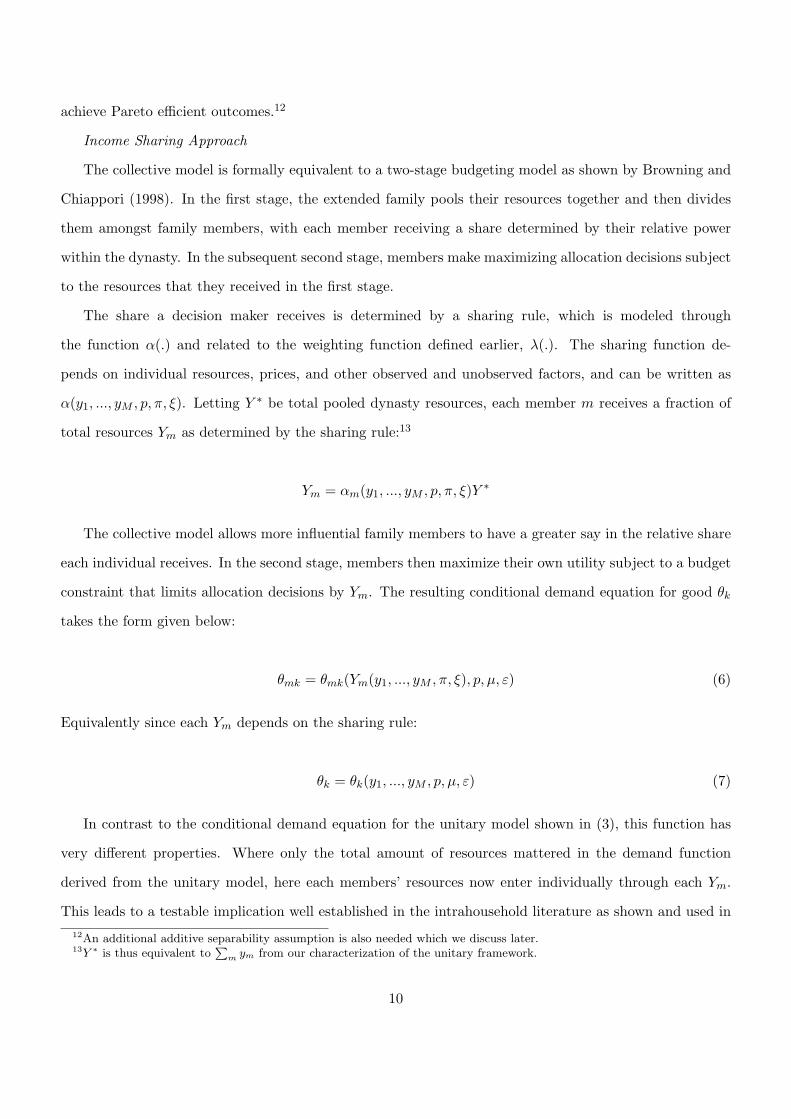
achieve Pareto efficient outcomes.12

Income Sharing Approach

The collective model is formally equivalent to a two-stage budgeting model as shown by Browning and

Chiappori (1998). In the first stage, the extended family pools their resources together and then divides

them amongst family members, with each member receiving a share determined by their relative power

within the dynasty. In the subsequent second stage, members make maximizing allocation decisions subject

to the resources that they received in the first stage.

The share a decision maker receives is determined by a sharing rule, which is modeled through

the function α(.) and related to the weighting function defined earlier, λ(.). The sharing function de-

pends on individual resources, prices, and other observed and unobserved factors, and can be written as

α(y1, ..., yM , p, π, ξ). Letting Y ∗ be total pooled dynasty resources, each member m receives a fraction of

total resources Ym as determined by the sharing rule:13

Ym = αm(y1, ..., yM , p, π, ξ)Y ∗

The collective model allows more influential family members to have a greater say in the relative share

each individual receives. In the second stage, members then maximize their own utility subject to a budget

constraint that limits allocation decisions by Ym. The resulting conditional demand equation for good θk

takes the form given below:

θmk = θmk(Ym(y1, ..., yM , π, ξ), p, µ, ε) (6)

Equivalently since each Ym depends on the sharing rule:

θk = θk(y1, ..., yM , p, µ, ε) (7)

In contrast to the conditional demand equation for the unitary model shown in (3), this function has

very different properties. Where only the total amount of resources mattered in the demand function

derived from the unitary model, here each members’ resources now enter individually through each Ym.

This leads to a testable implication well established in the intrahousehold literature as shown and used in12An additional additive separability assumption is also needed which we discuss later.13Y ∗ is thus equivalent to

Pm ym from our characterization of the unitary framework.

10

Chiappori (1992), Bourguigon et al. (1993), and Browning and Chiappori (1998) among others.

This test follows from the way individual resources only influence demand through the share of resources

an individual receives in the first stage, Ym. Chiappori and coauthors show that under the assumption of

Pareto efficiently, this implies that the ratio of marginal effects of one family member’s resources on good θk

to another member’s resources will be constant across goods. Intuitively, this comes from the specification

of equation (6), and an assumption of weak separability between factors which influence bargaining power

and others that influence demands. Any factor, such as ym, that affects the demand for θk only through

the share of resources received in the first stage, must affect all demands from the second stage in the same

way.

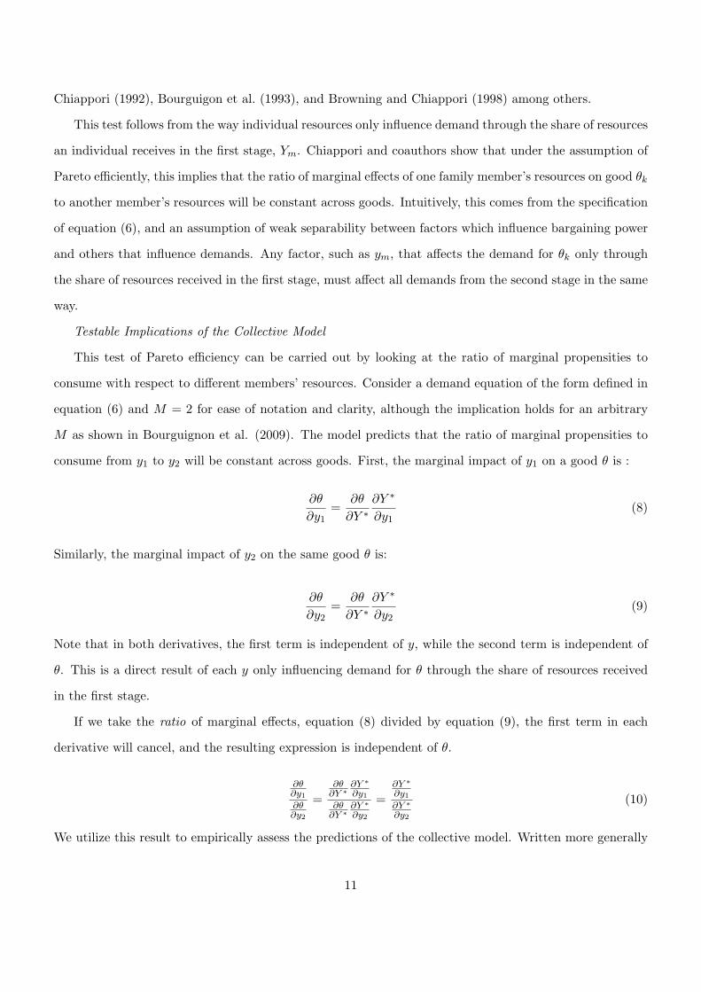
Testable Implications of the Collective Model

This test of Pareto efficiency can be carried out by looking at the ratio of marginal propensities to

consume with respect to different members’ resources. Consider a demand equation of the form defined in

equation (6) and M = 2 for ease of notation and clarity, although the implication holds for an arbitrary

M as shown in Bourguignon et al. (2009). The model predicts that the ratio of marginal propensities to

consume from y1 to y2 will be constant across goods. First, the marginal impact of y1 on a good θ is :

∂θ

∂y1=

∂θ

∂Y ∗∂Y ∗

∂y1(8)

Similarly, the marginal impact of y2 on the same good θ is:

∂θ

∂y2=

∂θ

∂Y ∗∂Y ∗

∂y2(9)

Note that in both derivatives, the first term is independent of y, while the second term is independent of

θ. This is a direct result of each y only influencing demand for θ through the share of resources received

in the first stage.

If we take the ratio of marginal effects, equation (8) divided by equation (9), the first term in each

derivative will cancel, and the resulting expression is independent of θ.

∂θ∂y1∂θ∂y2

=∂θ∂Y ∗

∂Y ∗

∂y1∂θ∂Y ∗

∂Y ∗

∂y2

=∂Y ∗

∂y1∂Y ∗

∂y2

(10)

We utilize this result to empirically assess the predictions of the collective model. Written more generally

11

for arbitrary goods j and k, and resources in control of m and n, a system of demand allocations is

compatible with Pareto efficiency if the ratio of marginal effects is constant across outcomes. That is:

∂θj

∂ym

∂θj

∂yn

=∂θk∂ym

∂θk∂yn

∀ j, k,m, n (11)

This restriction is a direct result of the two stage budgeting process. Since the distribution of dynasty

resources takes place before individual allocation decisions, factors which influence the share can only affect

allocations in a specific way in the second stage. With a conceptual model at hand, we move next to discuss

our empirical implementation, data and results.

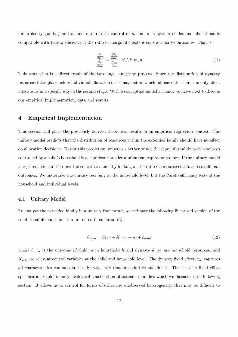
4 Empirical Implementation

This section will place the previously derived theoretical results in an empirical regression context. The

unitary model predicts that the distribution of resources within the extended family should have no effect

on allocation decisions. To test this prediction, we asses whether or not the share of total dynasty resources

controlled by a child’s household is a significant predictor of human capital outcomes. If the unitary model

is rejected, we can then test the collective model by looking at the ratio of resource effects across different

outcomes. We undertake the unitary test only at the household level, but the Pareto efficiency tests at the

household and individual levels.

4.1 Unitary Model

To analyze the extended family in a unitary framework, we estimate the following linearized version of the

conditional demand function presented in equation (3):

θmhd = β1yh +Xmhγ + ηd + εmhd (12)

where θmhd is the outcome of child m in household h and dynasty d, yh are household resources, and

Xmh are relevant control variables at the child and household level. The dynasty fixed effect, ηd, captures

all characteristics common at the dynasty level that are additive and linear. The use of a fixed effect

specification exploits our genealogical construction of extended families which we discuss in the following

section. It allows us to control for forms of otherwise unobserved heterogeneity that may be difficult to

12

model. These include, but are not limited to, common genetic background, dynasty wide preferences,

heredity factors, common prices, and expected future family resources.

The coefficient of interest in equation (12) is β1. The unitary model predicts that, conditional on total

dynasty resources, the share controlled by a child’s household should have no impact on θ. Since total

dynasty resources are captured through the fixed effect, ηd, the null of our test is:

H0 : β1 = 0 (13)

Thus, if the estimated β1 is statistically different from zero, we are able to reject the unitary model.

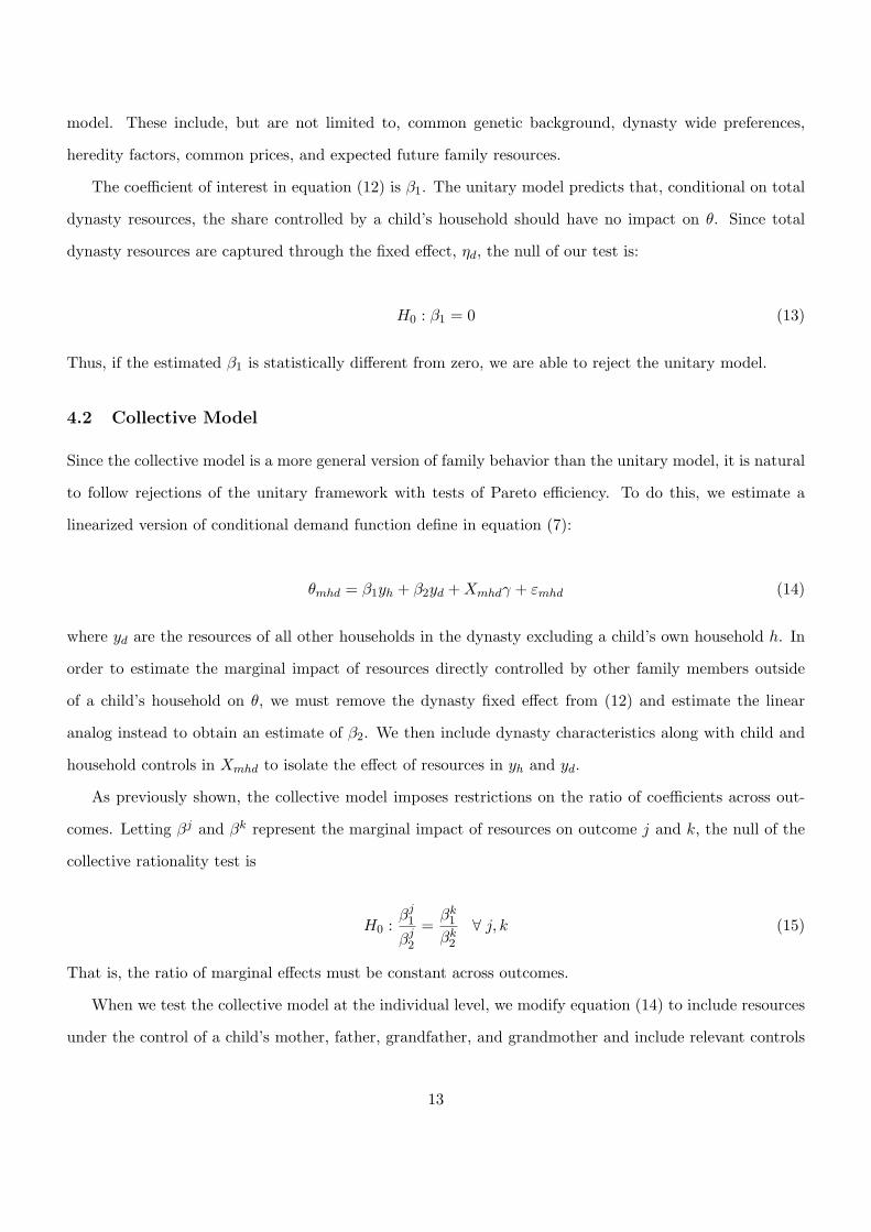
4.2 Collective Model

Since the collective model is a more general version of family behavior than the unitary model, it is natural

to follow rejections of the unitary framework with tests of Pareto efficiency. To do this, we estimate a

linearized version of conditional demand function define in equation (7):

θmhd = β1yh + β2yd +Xmhdγ + εmhd (14)

where yd are the resources of all other households in the dynasty excluding a child’s own household h. In

order to estimate the marginal impact of resources directly controlled by other family members outside

of a child’s household on θ, we must remove the dynasty fixed effect from (12) and estimate the linear

analog instead to obtain an estimate of β2. We then include dynasty characteristics along with child and

household controls in Xmhd to isolate the effect of resources in yh and yd.

As previously shown, the collective model imposes restrictions on the ratio of coefficients across out-

comes. Letting βj and βk represent the marginal impact of resources on outcome j and k, the null of the

collective rationality test is

H0 :βj1βj2

=βk1βk2

∀ j, k (15)

That is, the ratio of marginal effects must be constant across outcomes.

When we test the collective model at the individual level, we modify equation (14) to include resources

under the control of a child’s mother, father, grandfather, and grandmother and include relevant controls

13

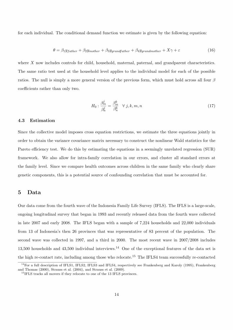
for each individual. The conditional demand function we estimate is given by the following equation:

θ = β1yfather + β2ymother + β3ygrandfather + β4ygrandmother +Xγ + ε (16)

where X now includes controls for child, household, maternal, paternal, and grandparent characteristics.

The same ratio test used at the household level applies to the individual model for each of the possible

ratios. The null is simply a more general version of the previous form, which must hold across all four β

coefficients rather than only two.

H0 :βjm

βjn=βkmβkn

∀ j, k,m, n (17)

4.3 Estimation

Since the collective model imposes cross equation restrictions, we estimate the three equations jointly in

order to obtain the variance covariance matrix necessary to construct the nonlinear Wald statistics for the

Pareto efficiency test. We do this by estimating the equations in a seemingly unrelated regression (SUR)

framework. We also allow for intra-family correlation in our errors, and cluster all standard errors at

the family level. Since we compare health outcomes across children in the same family who clearly share

genetic components, this is a potential source of confounding correlation that must be accounted for.

5 Data

Our data come from the fourth wave of the Indonesia Family Life Survey (IFLS). The IFLS is a large-scale,

ongoing longitudinal survey that began in 1993 and recently released data from the fourth wave collected

in late 2007 and early 2008. The IFLS began with a sample of 7,224 households and 22,000 individuals

from 13 of Indonesia’s then 26 provinces that was representative of 83 percent of the population. The

second wave was collected in 1997, and a third in 2000. The most recent wave in 2007/2008 includes

13,500 households and 43,500 individual interviews.14 One of the exceptional features of the data set is

the high re-contact rate, including among those who relocate.15 The IFLS4 team successfully re-contacted14For a full description of IFLS1, IFLS2, IFLS3 and IFLS4, respectively see Frankenberg and Karoly (1995), Frankenberg

and Thomas (2000), Strauss et al. (2004), and Strauss et al. (2009).15IFLS tracks all movers if they relocate to one of the 13 IFLS provinces.

14

90.6% of the living IFLS1, 2 and 3 households, and 87% of original living IFLS1 respondents. These rates

are as high, or higher, than most longitudinal surveys in the United States and Europe.

Constructing the Extended Family

We follow a similar method to that used by Altonji et al. (1992) in linking households to their extended

families. Similar to the Panel Study of Income Dynamics data in the US, which Altonji et al. (1992) used,

the structure of the IFLS panel allows us to identify dynasties using family members who have left IFLS

households and been followed by the survey. Starting from a base household, when a member leaves to form

a new household, often through marriage, the newly formed unit is located and becomes part of the IFLS

in all subsequent waves. We thereby create IFLS dynasties by linking these split-off households back to

their original root. Although we do not observe the full genealogical family tree, it is a rich characterization

of the extended family. One advantage of linking the data in this way is it allows us to empirically sweep

out unobserved heterogeneity at the extended family level through the use of dynasty fixed effects in our

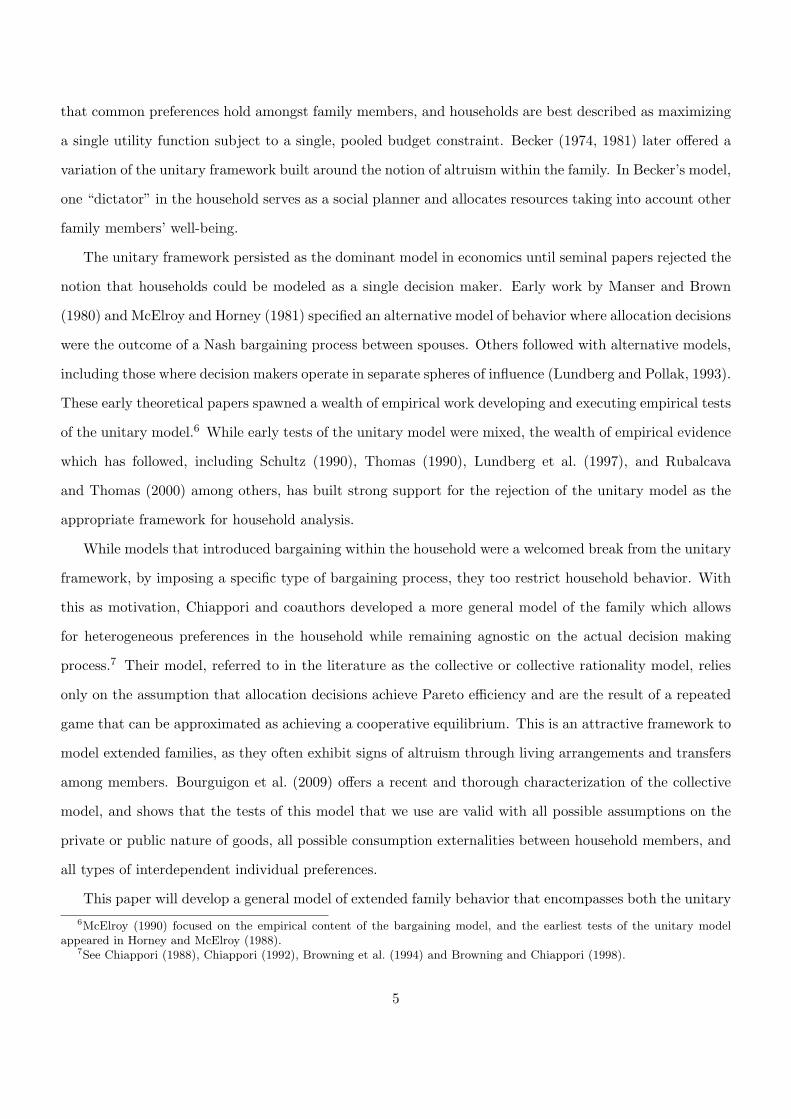
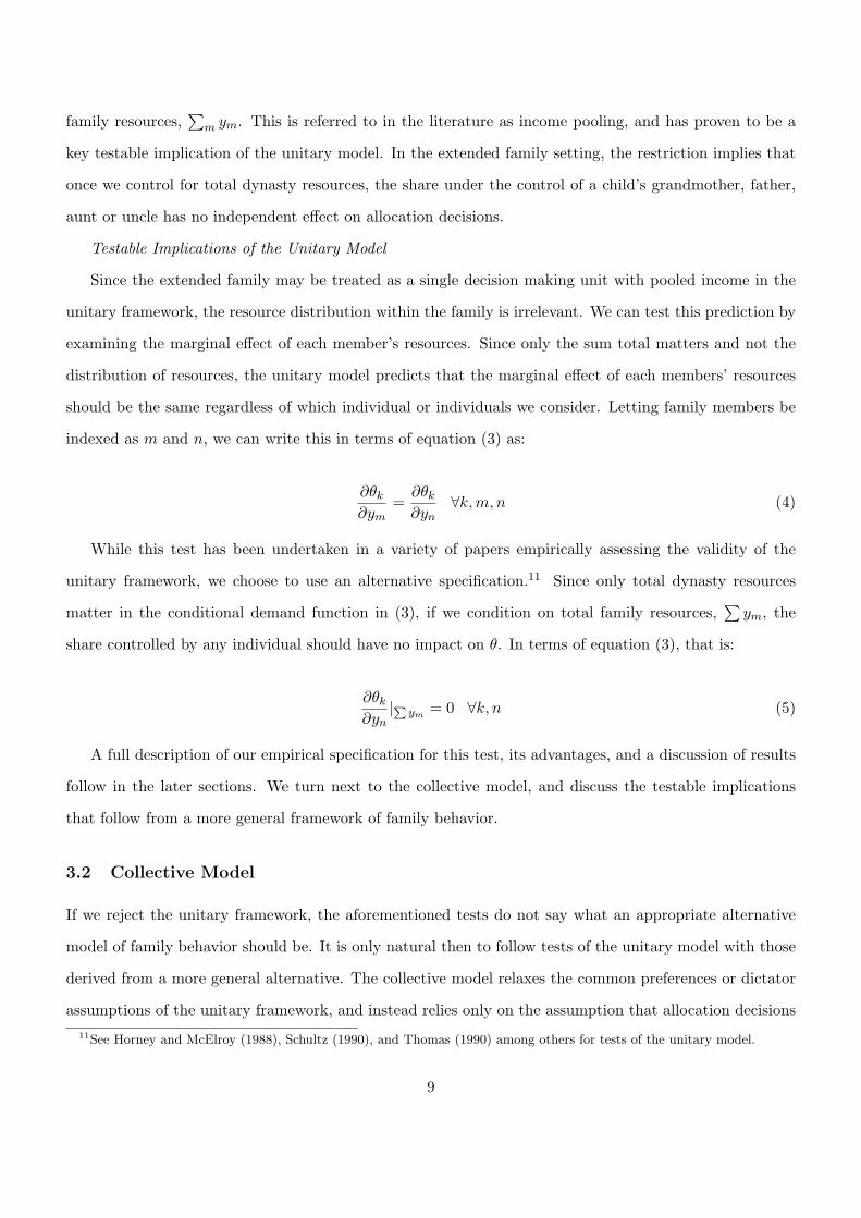
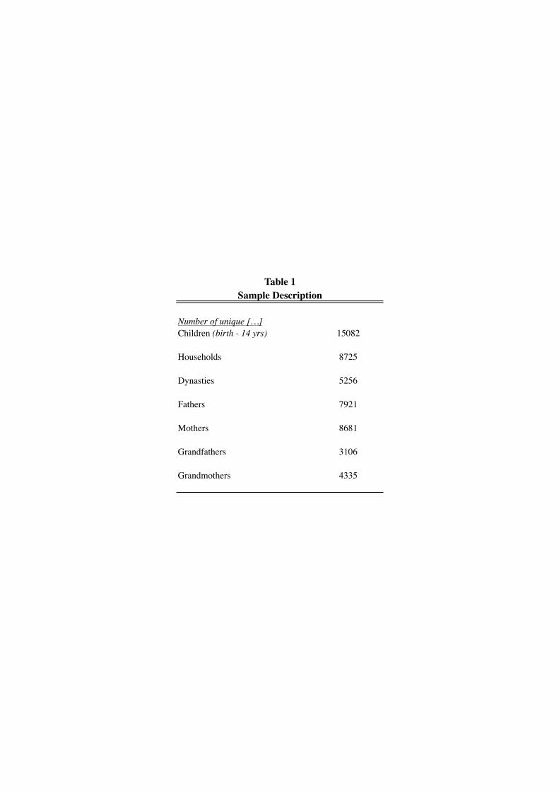
tests of the unitary model. Table 1 provides an overview of the number of children, households, dynasties,

parents and grandparents in our sample.

Health and Development Outcomes

We look at three markers of child health and development in our estimation; height-for-age, early

school attendance, and cognition.16 We convert height to age and gender specific z-scores using the 2000

Center for Diseases Control growth tables, which uses a representative, well-nourished child in the United

States as the norm. As mentioned earlier, height is an accepted long-run marker of human capital, and

a stock variable embodying nutritional investments made during early childhood.17 While a variety of

nutrition and medical studies have found the heredity of height to be approximately 75 to 80 percent (e.g.

Silventoinen et al., 2000), the remaining 20 - 25 percent is a reflection of environmental factors during

pregnancy and early life, including maternal smoking, nutritional intake, the disease environment, and

health insults. The effect of resources on height have been shown to be most influential in the early years

of life (Alderman et al., 2006), so when considering height-for-age, we present results for children from six

month to age four separately from those children age five to age nine.

We also examine early school attendance as a dependent variable and marker of human capital accu-16The IFLS contains a wide range of potential outcomes, and we have also considered BMI, weight-for-age, an interviewer’s

health assessment, school enrollment, and others. Results using outcomes besides those presented here are consistent withthose shown and available upon request.

17See, for example, Alderman et al. (2006), Strauss and Thomas (1998), Mwabu (2008) and Waterlow et al. (1977).

15

mulation. Although in a different context, work examining the causal effect of early start programs in the

United States show a significant positive effect of early school attendance on markers such as high school

completion, college attendance, and later life outcomes (e.g. Garces et al., 2002). We simply follow the

chain of reasoning that attending school at an early age will offer those students an advantage in later life.

In particular, we use whether or not a child ever attended kindergarten in a sample of children age six to

fourteen.18

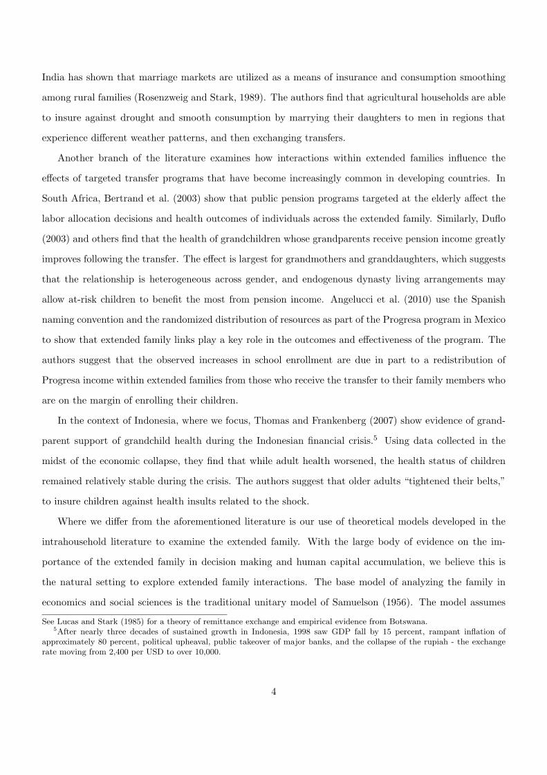
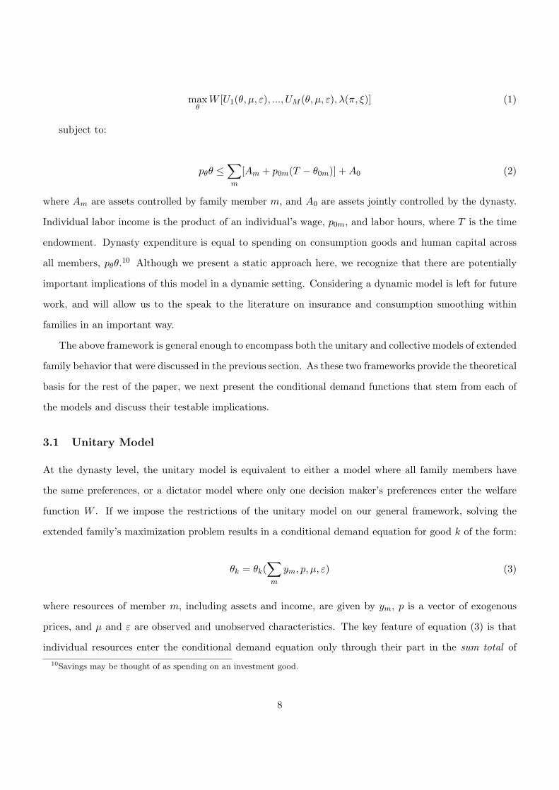
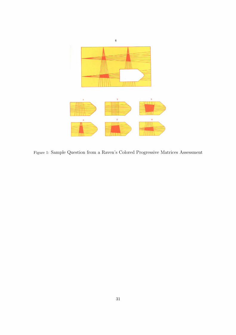
Finally, we take advantage of a unique and underutilized module in the IFLS which measures cognition

through a non-verbal assessment. Individuals age seven to fourteen were given a test comprised of twelve

Raven’s Colored Progressive Matrices (CPM) questions and five math problems to assess their cognitive

function.19,20 Since the CPM is an metric not often used in the economics literature, we have included a

sample question as Figure 1.

The CPM assessment is commonly used in medicine and psychology as a measure of general intelligence,

and is accepted as the single best measure of Spearman’s general intelligence factor g (Kaplan and Saccuzzo,

1997). The presence of an accepted objective measure of cognition is one of the great benefits of IFLS.

Since the CPM test is based on pattern recognition, there is a natural positive correlation with age among

the children respondents from age seven to fourteen. We considered standardizing the scores by age, but

instead choose to use the percent correct as the dependent variable, and control for age in a flexible way

in our regressions. The results are not sensitive to this specification.

Distribution Factors

To test the theoretical predictions of the two models, we need a measure of relative power that influences

the bargaining process within a family. In our estimation, we associate power with the value of assets

under the control of each household, or individual, within a dynasty. The IFLS includes a detailed roster

of assets broken into thirteen categories.21 We consider all household assets excluding housing and land to

be considered liquid, and focus on those in our estimation.

One of the benefits of focusing on assets is the ability to conduct our analysis at both the household and

individual level. The IFLS is unique among major surveys in its inclusion of questions about individual18This is an indicator equal to one if a child is currently enrolled in kindergarten or ever was.19A similar, but longer, test was given to individuals between the ages of fifteen and twenty four.20The CPM is designed particularly for children. For a background on the Raven’s Standard Progressive Matrices (SPM)

test, see Raven (1958), or for a more recent treatment, see Raven (2000).21In the order asked, they are: house occupied by the household, other house, non-agricultural land, poultry, livestock,

hard stem plant, vehicles (cars, boats, bicycles and motorbikes), household appliances, savings/certificate of deposit/stocks,receivables, jewelry, household furniture and utensils, and other.

16

resources within a household. The questionnaire asks each adult member of a household age 15 and above

about the total value of household assets in each of the thirteen categories, and the share which they

and others within and outside the household control. We obtain our measures of individual resources

by multiplying the reported value of an asset by an individual’s share, and then sum over the liquid

asset categories. Since we often have different and inconsistent answers for individuals within the same

household, there are plausibly many models for constructing individual assets. One possibility would be to

trust the household head’s response as the correct depiction of the asset distribution, and create individual

assets from their response on others’ ownership. Instead, we choose to use each individual’s own response

if available.22 We chose this method after observing that spouses systematically underreport the value of

assets held by their partner. This pattern is particularly true for husbands’ reports on their wives’ assets.

While we begin with household level analysis as a firsts step and to be consistent with the literature,

utilizing individual level data has many advantages. Chief among these is the ability to avoid concerns as-

sociated with endogenous living arrangements that plague analysis at the household level. Using individual

level data allows us to compare resources of different family members both within and across households.

This lets us examine any sharing and insurance that happens between extended family members, but within

a household unit. For instance, if the primary means of sharing and consumption smoothing amongst fami-

lies happens through co-residence patterns, ie. grandmothers living with young children, this will be missed

using household level data, but visible at the individual level.

However, focusing on assets is certainly not without risk, and our results come with the caveat that

assets themselves may be the outcomes of an extended family allocation process and pose endogeneity

concerns. However, they do serve a distinct improvement over the common practice of utilizing expenditure,

and allow us to look at the results and tests at the individual level. To be consistent with the literature,

we have done tests of the unitary and collective models with household per capita expenditure instead of

assets and include a discussion of the results in Appendix A. We maintain a preference for assets, as they

reflect a closer, although still imperfect, representation of long-run resources, which is what our testable

implications are founded upon. Without additional restrictive assumptions, expenditure should be seen

as the outcome of the bargaining process, not a distribution factor which influences the first stage of the

budgeting process.

We include a variety of control variables on the right hand side to isolate the resource effects in our22If an individual’s own response is not available due to refusal or other reason, we use the response from a spouse.

17

asset measures. At the child level, we include gender and age, using indicator variables for each age. This

is a flexible way to capture any significant differences between older and younger children in the measures

of health and human capital, including those mentioned with the cognitive score. We also condition on

whether the child lives with their mother and father, since it is likely that those children who co-reside

with their parents experience different environments and familial interactions that those that do not.

At the household, and dynasty level when appropriate, we include demographic controls including

household size and composition variables. For composition, we include the number of household members

divided into five distinct groups: children, prime age males, prime age females, senior males, and senior

females.23 In regressions which look at the household and dynasty level, we control for age and education

of the household and dynasty head, and for regressions at the individual level, we include the age and

education of both parents and grandparents. We code education as the highest level completed rather

than years, although the results are not sensitive to this specification.24 We also control for location with

province indicators, and include an indicator for whether the household is located in an urban or rural

region to account for the fact that resources are systematically higher in urban areas.

Finally, to control for the genetic component of height, we include both mother’s and father’s height.

Since adult height is correlated with labor market outcomes, this also controls for labor market factors

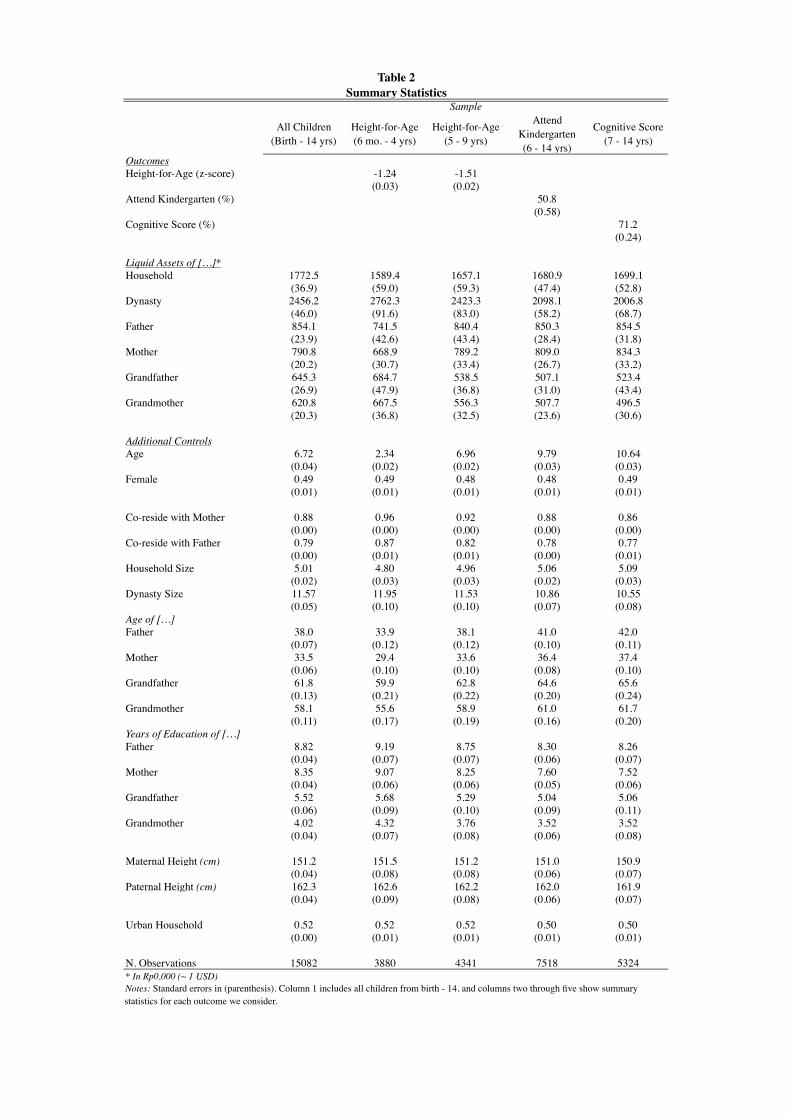
not captured by parental education. Summary statistics reporting means and standard errors are shown

in Table 2. Because we consider different samples due to the relevance of our outcomes for different age

groups, we present both summary statistics for all children from birth to 14 in column one, and for each

of the four groups in columns two through five. Looking at our outcomes of interest, we see that height

for age in young children has a mean of -1.2 and -1.5 in older children, implying that children in Indonesia

are more than one standard deviation shorter than well-nourished children of the same age and gender in

the United States. We also see that approximately half of the children between 6 and 14 currently attend

or attended kindergarten, and the mean score on the cognitive assessment is seventy one percent correct.

Liquid assets are reported in 10,000 rupiah, which is approximately 1 USD. Dynasty assets are defined

as total assets of the extended family less an individual’s specific household assets. Table 2 shows that

the majority of extended family resources are controlled by those outside a given child’s household, with23We define prime age as 15-55 and senior as 56 and above. Results are not sensitive to these cut-offs. Since we include

household size in our regressions, we have to exclude one category to avoid multicollinearity - we choose senior women.24We include education through dummies for each of the following levels: no education, kindergarten, elementary, junior

high, senior high, and greater than senior high.

18

a given household owning approximately 40 percent of total dynasty resources. We also see that the value

of assets controlled by fathers is more than mothers, as is grandfathers compared with grandmothers.

With a theoretical model at hand, and a knowledge of the data and empirical specification, we move

next to discuss our results.

6 Findings

In this section, we present and discuss our empirical results in the context of the unitary and collective

models. Throughout, we refer to tables 3 through 7, which report β estimates.25 For analysis at the

household level, we use a logarithmic transformation of asset levels. However, for analysis at the individual

level, there are multiple reports of zero asset holdings. To address this problem, we use a quartic root

transformation, which approximates the common logarithmic transformation but is defined at zero while

the log is not. This has the advantage of not dropping observations as the result of the log transformation.

We maintain logs at the household level for ease of interpretation, and because there are not a significant

amount of zero-valued observations to warrant concern.26 In the tables that show regression results, column

one for each outcome shows the combined effect for both boys and girls, while column two includes results

from a similar model, but one that is fully interacted with gender to allow for varying effects amongst boys

and girls. This allows us to assess the predictions of the unitary and collective models differently for each

gender. The relevant coefficient, and ratio where applicable, for boys is reported on the same line as the

main effect, and the relevant coefficient for girls is the sum of the main and interaction effects.

6.1 Tests of the Unitary Model

To begin, Table 3 shows results for tests of the unitary model from equation (12) using dynasty fixed

effects to sweep out factors that are common, additive and linear at the dynasty level. Since we use a

logarithmic transformation, the coefficients may be interpreted in the usual approximation of percentage

changes. However, the main interpretation and inference relies only on the sign and significance regardless

of the transformation; when the value of resources controlled by a child’s own household increases, we see a25Due to space and clarity considerations, only the β coefficients are reported here. Results including all controls are

available upon request.2699.2% of all households report non-zero values for liquid asset holdings. The remaining 0.8% are not dropped, but instead

we replace the 0 value with the mean and include an indicator in the regression noting replacement.

19

significant increases in all three of our health and human capital outcomes. In terms of gender differentials,

we do not see any significant differences between boys and girls.27

These results reject the restrictions of the unitary model, which predicts that all of the reported

coefficients in Table 3 be zero. We reject the notion that the share of resources controlled by an individual

household have no impact on child outcomes once we condition on total dynasty resources. This suggests

that the unitary model is not an appropriate representation of the extended family. This does not come as

a surprise, and is a consistent finding in the intrahousehold literature. However, since the collective model

subsumes the unitary, establishing a rejection of the unitary model is a natural first step before testing the

more general implications of Pareto efficiency.

6.2 Tests of the Collective Model

Household Pareto Efficiency Regressions

In order to test Pareto efficiency between households and the remainder of the extended family, it is

necessary to remove the dynasty fixed effect from the previous model, and estimate equation (14) instead.

Doing so allows us to estimate the marginal effect of resources controlled by non co-resident family members

outside of a child’s own household. These results are shown in Table 4, which reports estimates that are

similar to the fixed effects specification for household resources. More importantly, it provides evidence

that extended family resources do have an impact on human capital accumulation of young children. This

is seen most clearly in early school attendance and cognitive scores, where increasing the value of assets held

by non co-resident family members increases enrollment and cognitive achievement. Dynasty resources are

also also positive and significant in regressions examining height-for-age, albeit only at 10 percent. This is

evidence of inter-dynasty transfers, and may be similar to the pattern shown in Mexico by Angelucci et al.

(2010). The coefficients for the other outcomes are positive yet imprecisely estimated. The ratios reported

in the lower panel of Table 4 are obtained using the delta method, and show that the effects of household

resources are relatively larger than those of dynasty resources.

Household Pareto Efficiency Tests

Table 5 shows the results of the cross equation, nonlinear Wald tests of Pareto efficiency described in

(15). When we execute these tests, we combine our two height-for-age samples into one sample of children27The one exception is with older children’s height-for-age. Investigation into any differential biology of growth for Indonesian

boys and girls not accounted for in the standardization of the z-scores did not lend any support to a substantial difference.

20

six months to age nine. The coefficient estimates for the two different age groups are not statistically

different from each other, and combining also allows for greater precision in our ratio tests. The three

ratios that we use are reported in panel A of Table 5, and p-values from the nonlinear Wald tests appear in

panel B. The first three rows of panel B show pairwise test of the restrictions for the outcome in the first

column and the second column. Although the model implies the restrictions hold across all three outcomes,

we report these pairwise tests of efficiency so as to not miss any possible rejections on a case-by-case basis

in addition to the overarching test. For example, the first value in Panel B of 0.50 suggests that we cannot

reject that the ratio of household to dynasty resources is the same for height-for-age and early school

attendance. The final row shows the test for equality across all three ratios.

We include the second and third columns in panel B of Table 5 to examine potential gender differences

in efficient allocation. Our results suggest that we are not able to rule out Pareto efficiency in any of the

tests, including those differentiating by gender. All of the p-values are well above any reasonable range

of rejection. Thus, while we are able to reject the unitary model of the extended family, we are not able

to reject that extended families allocate resources Pareto efficiently, and may be appropriately modeled

as a collective unit.28 All of the ratios are statistically indistinguishable and in the range of 2.52 to 4.01.

Economically, this implies that the marginal impact of a child’s own household resources is approximately

two to four times larger than resources controlled by other dynasty members.

Individual Pareto Efficiency Regressions

Having rejected the unitary mode but not tests of collective rationality at the household level, we

next look within the extended family at the individual level. These results provide empirical evidence

on the importance of intergenerational transfers in child development. As mentioned earlier, that we

provide individual level results for members within an extended family is a unique feature of our data and

paper. Although there is a slightly more nuanced interpretation due to the quartic root specification, the

main implications and interpretation based on sign and significance is still valid. Our findings, shown in

Table 6, suggest that children significantly benefit from resources controlled by their mothers. We see this

specifically in height-for-age and cognitive scores. Since these are both markers of long-run human capital,

this finding suggests persistent benefits for those children in families where mothers control a substantial

amount of resources. The result that children benefit as their mothers gain is consistent with previous28It is important to note that although we find no evidence of differences between girls and boys in terms of efficiency,

this does not rule out different behavior or patterns of allocation, only that the outcomes for both boys and girls can becharacterized by an efficient allocation process.

21

findings examining the allocation of resources toward women and children (e.g. Thomas, 1990; Duflo,

2003).

While the result concerning mother’s resources is the same for kindergarten attendance, a more revealing

pattern exists with early school attendance. Mother’s assets show a large, positive and significant effect,

but there are also positive and significant effects for father’s and grandmother’s assets. This may be related

to time use, in that wealthier dynasties may not need their children to work in home production and can

send them to school instead. More importantly, it shows specific signs of intergenerational interaction, as

the effect of grandmothers’ assets is on the order of fathers’ resources. Father’s assets are also significant

in early height-for-age.

Individual Pareto Efficiency Tests

The final table of our results, Table 7, shows the individual level analog to the household Pareto

efficiency tests in Table 5. Again, the table shows p-values from the nonlinear Wald test of the restrictions

imposed by the collective model. Since we look at four different resource coefficients (resources controlled by

mothers, fathers, grandmothers, and grandfathers), there are six pairwise ratios to test, as well as equality

across all six for each pair of outcomes, and equality of all six ratios across all three outcomes. In Table 7

the individual listed in the column is the denominator and the individual in the row is the numerator. For

example, 0.37 is the p-value of the test comparing the marginal impact of father’s resources to mother’s

resources between height-for-age and early school attendance. The value suggests that we cannot reject

the null with any reasonable confidence level. Panels B and C report p-values for tests on boys and girls

separately, but we find no differences in the interpretation of the model. There is only one test where

we reject Pareto efficiency at the 5 percent confidence level, for mother and grandfather assets comparing

kindergarten attendance and cognitive scores in the tests which combine boys and girls. However, this is

only one rejection out of 66 tests in table 7 and is not rejected in either of the gender specific tests. In all

others cases, we cannot rule out that extended families behave in a Pareto efficient manner.

6.3 Robustness Checks

Our rejections of the unitary model and failure to reject Pareto efficiency are robust to a variety of different

outcomes, empirical specifications and sample stratifications. We have already presented results which test

Pareto efficiency separately for boys and girls, and saw no difference in our results. The same holds

true for examining other health and education outcomes in the IFLS including BMI, weight-for-age, an

22

interviewer’s health assessment, school enrollment and others. This section briefly discusses additional

specification checks and sensitivity analysis which we completed.29

To start, the regressions in equations (12) and (14) that we use to estimate the unitary and collective

models are linear in the log or quartic root of assets. We also examined a variety of specifications for our

empirical tests that allowed assets to enter in non-linear forms including quadratic and cubic polynomials

and splines. Neither rejections of the unitary model nor failures to reject Pareto efficiency were sensitive to

these alternative specifications, and we were not able to rule out linearity through the use of specification

tests. We also attempted to address the incomplete nature of our constructed extended families. Because

we base dynasties on a collection of split-off households, our sample does not include any children who are

in the extended family but outside of IFLS households. To assess whether it matters if the root household

is on the maternal or paternal side of the dynasty, we separately estimated models for families where the

mother in a new household is an IFLS panel member compared with those where the father is an IFLS

split-off. Again, we found no significant differences.

To test whether Pareto efficiency could be rejected for different sub-groups of the population, we

stratified out sample on a variety of demographic factors. This allowed us to examine if Pareto efficiency

would be rejected for families with different demographic composition, education levels, or greater physical

distance between members.30 We stratified the sample based on the number of household and dynasty

members, the number of children within a household or dynasty, and the number of other children within

the household or dynasty within 3 years of a child’s age to assess whether competing over resources has

any impact on efficiency. We also examined whether stratifying the sample based on urban and rural

households, geographic distance to other family members, the age of a child’s mother and father, and the

mean and maximum levels of education among adults in the family had any impact on our results. Across

all stratifications, we found no rejections of Pareto efficiency.

All of the results presented here use data from the 2007 wave of the IFLS. We have also made use of

the IFLS panel to verify our current results.31 Reestimating the models using data from the 2000 wave of29To conserve space, results discussed in this section are omitted from the paper, but they are available from the authors

upon request. They will also be available online at www.econ.duke.edu/ drl13/extendedfamilies30It may be more difficult for extended family members that are not located near each other to exchange transfers, for

example.31There are some challenges using the full panel in our research design. Because families expand over the course of the

survey, the number of dynasties with split-off households is much smaller in earlier waves of the survey. This makes it difficultto estimate models that rely on variation at the dynasty level. However, the 1997 and 2000 wavs of the survey do have lowerlevels of attrition, which makes analyzing them attractive. The IFLS2 in 1997 and the IFLS3 in 2000 recontacted 95 percentof living IFLS1 households, while IFLS4 recontacted 91 percent.

23

the IFLS provides a verification that our results are not specific to the one wave we choose to use. The

estimation results from 2000 are consistent with those shown here. We again reject the unitary model and

fail to reject Pareto efficiency. Moreover, the coefficient estimates are also remarkably similar across waves.

We also considered combining data across waves to form a panel. This would allow us to estimate

models which control for dynasty fixed effects in all regressions, not only those testing the unitary model.

Combining the 2000 and 2007 samples, for instance, would mean that we had data where dynasty assets

vary across time. However, the sample of individuals for which these models is identified is small and

selected. Consider the model which estimates the impact of household and dynasty resources on cognitive

scores, shown in equation (14), as an example.32 The cognitive score outcome is defined for children age

7-14. In order to identify the effect of dynasty resources independent of a dynasty fixed effect, we would

require there to be multiple children in the extended family between 7 and 14 in both the 2000 and 2007

waves of the survey. Furthermore, the children would have to be in different households within the extend

family. This is a small and selected subset of the children in our sample.

We do not believe our results are unreasonable. A wealth of literature supports the importance of the

extended family in human capital accumulation, and many papers have shown allocations to be Pareto

efficient at the household level.33 Our analysis has extended these results to the extended family which

plays an important role in child development. We summarize and offer ideas for future work to strengthen

our results as we conclude.

7 Conclusion

Transfers between extended family members are thought to be an important part of the lives of many

individuals, yet there is little known empirically on the subject. This paper offers an improved way to

specifically understand the role that interactions between extended family members play in child devel-

opment. Through the use of general models of family behavior, we show that the unitary model is not a

valid characterization of the relationship between co-resident and non co-resident family members. How-

ever, we are not able to rule out that allocation decisions achieve Pareto efficiency. This is true at the

household level, and the unique nature of the IFLS allows us to show that it is true at the individual level32The proposed estimation equation would then be θmhd = β1yh+β2yd+Xmhdγ+νd+εmhd where νd captures time-invariant

observed and unobserved heterogeneity at the dynasty level.33See, among others, Bourguigon et al. (1993).

24

as well. These results highlight the role and importance of the extended family in early life human capital

accumulation.

Using our framework to look at adult health outcomes may offer an interesting complement to these

results. If extended families focus on child but not adult health, this may be an area where Pareto efficiency

among families is actually rejected. We will examine this possibility in future work. The results presented

here are important for understanding intra-family relationships and generational exchange. We show that

even in a setting where market imperfections are often thought to disrupt exchange, extended families are

able to allocate resources efficiently to aid in the health and development of their youngest generation.

25

References

Alderman, H., J. Hoddinott, and B. Kinsey, “Long Term Consequences of Early Childhood Malnu-

trition,” Oxford Economic Papers, 2006, 58, 450–474.

Almond, D., “Is the 1918 Influenza Pandemic Over?,” Journal of Political Economy, 2006, 144, 672–712.

, L. Edlund, H. Li, and J. Zhang, “Long-term Effects of the 1959-1961 China Famine: Mainland

China and Hong Kong,” 2007. Mimeo.

Altonji, J., F. Hayashi, and L. Kotlikoff, “Is the Extended Family Altruistically Linked? Direct Tests

Using Micro Data,” The American Economic Review, 1992, 82 (5), 1177–1198.

Angelucci, M., G. DeGiorgi, M. Rangel, and I. Rasul, “Family Networks and School Enrolment:

Evidence from a Randomized Social Experiment,” Journal of Public Economics, May 2010, Forthcoming.

Becker, G., “A Theory of Social Interactions,” The Journal of Political Economy, November 1974, 82

(6), 1063–1093.

, A Treatise on the Family, Cambridge, Massachusetts: Harvard University Press, 1981.

Bertrand, M., S. Mullainathan, and D. Miller, “Public Policy and Extended Families: Evidence

from Pensions in South Africa,” The World Bank Economic Review, 2003, 17 (1), 27–50.

Bianchi, S., J. Hotz, K. McGarry, and J. Seltzer, “Intergenerational Ties: Alternative Theories,

Empirical Findings and Trends, and Remaining Challenges,” in A. Booth, N. Crouter, S. Bianchi, and

J. Seltzer, eds., Intergenerational Caregiving, Urban Institute, 2008, pp. 3–44.

Bourguigon, F., M. Browning, and P. A. Chiappori, “Efficient Intra-Household Allocations: A

General Characterization and Empirical Tests,” The Review of Economic Studies, 2009, 76, 503–528.

, , , and V. Lechene, “Intra Household Allocation of Consumption: a Model with some evidence

from French data,” Annales D’Economie et de Statistique, 1993, 29, 137–156.

Browning, M. and P. A. Chiappori, “Efficient Intra-Household Allocations: A General Characteriza-

tion and Empirical Tests,” Econometrica, 1998, 66 (6), 1241–1278.

26

, F. Bourguigon, P. A. Chiappori, and V. Lechene, “Incomes and Outcomes: A Structural Model

of Intra-Household Allocation,” Journal of Political Economy, 1994, 102 (6), 1067–1096.

Chiappori, P. A., “Rational household labor supply,” Econometrica, 1988, 56 (1), 63–89.

, “Collective Labor Suplly and Welfare,” Journal of Political Economy, 1992, 100 (3), 437–467.

Cox, D., “Private Transfers within the Family: Mothers, Fathers, Sons and Daughters,” in A. Munnell

and A. Sunden, eds., Death and Dollars: The Role of Gifts and Bequests in America, Washington, D.C.:

Brookings Institution Press, 2003, pp. 168–217.

Dauphin, A. and B. Fortin, “A Test of Collective Rationality for Multi-Person Households,” Economics

Letters, 2001, 71, 211–216.

Duflo, E., “Grandmother and Granddaughters: Old-Age Pensions and Intrahousehold Allocations in

South Africa,” World Bank Economic Review, 2003, 17 (1), 1–25.

Frankenberg, E. and D. Thomas, “The Indonesia Family Life Survey (IFLS): Study Design and Results

from Waves 1 and 2,” Technical Report, Rand Corporation March 2000.

and L. Karoly, “The 1993 Indonesia Family Life Survey: Overview and Field Report,” Technical

Report, Rand Corporation November 1995.

Garces, E., D. Thomas, and J. Currie, “Longer-Term Effects of Head Start,” The American Economic

Review, September 2002, 92 (4), 999–1012.

Horney, M. J. and M. McElroy, “The Household Allocation Problem: Empirical Results from a

Bargaining Model,” Research in Population Economics, 1988, 6, 15–38.

Kaplan, R. and D. Saccuzzo, Psychological testing: Principles, Applications, and Issues, 4th ed., Pacific

Grove, CA: Brooks/Cole, 1997.

Lucas, R. E. B. and O. Stark, “Motivations to Remit: Evidence from Botswana,” The Journal of

Political Economy, October 1985, 93 (5), 901–918.

Lundberg, S. and R. Pollak, “Seperate Spheres Bargaining and the Marriage Market,” Journal of

Political Economy, 1993, 101 (6), 988–1010.

27

, , and T. Wales, “Do Husbands and Wives Pool their Resources? Evidence from the United

Kingdom Child Benefit,” Journal of Human Resources, 1997, 32 (3), 463–480.

Manser, M. and M. Brown, “Marriage and Household Decision Making: A Bargaining Analysis,”

International Economic Review, 1980, 21 (31-34).

McElroy, M., “The Empirical Content of Nash-bargained Household Behavior,” Journal of Human Re-

sources, 1990, 25, 559–583.

and M. J. Horney, “Nash-Bargained Household Decisions: Toward a Generalization of the Theory

of Demand,” International Economic Review, 1981, 22, 333–347.

Meng, X. and N. Qian, “The Long Run Health and Economic Consequences of Famine on Survivors,”

2006. IZA Discussion Papers.

Mwabu, G., “Health Economics for Low-Income Countries,” in T. Paul Schultz and J. Strauss, eds.,

Handbook of Development Economics, Vol. 4, North-Holland, 2008.

Rangel, M., “Efficient Allocation of Resources within Extended-Family Households: Evidence from De-

veloping Countries,” December 2004. Harris School of Public Policy Working Paper.

Raven, J., “The Raven’s Progressive Matrices: Change and stability over culture and time,” Cognitive

Psychology, 2000, 41, 1–48.

Raven, J. C., The Standard Progressive Matrices, San Antonio, TX: Harcourt Assessment, 1958.

Rosenzweig, M. and O. Stark, “Consumption smoothing, migration and marriage: evidence from rural

India,” The Journal of Political Economy, August 1989, 97 (4), 905–926.

Rubalcava, L. and D. Thomas, “Family Bargaining and Welfare,” July 2000. California Center for

Population Research Working Paper.

, G. Teruel, and D. Thomas, “Investments, Time Preferences, and Public Transfers Paid to Women,”

Economic Development and Cultural Change, 2009, 57 (3), 507–538.

Samuelson, P., “Social Indifference Curves,” Quarterly Journal of Econoimcs, 1956, 70 (1), 1–22.

28

Schultz, T., “Testing the Neoclassical Model of Family Labor Supply and Fertility,” Journal of Human

Resources, Fall 1990, 25 (4), 599–634.

Silventoinen, K., J. Kaprio, E. Lahelma, and M. Koskenvuo, “Relative effect of genertic and

environmental factors on body height: differences across birth cohorts among Finnish men and women,”

American Journal of Public Health, 2000, 90, 627–630.

Strauss, J. and D. Thomas, “Health Over the Life Course,” in T. Paul Schultz and J. Strauss, eds.,

Handbook of Development Economics, Vol. 4, New Palgrave, 2008.

and Duncan Thomas, “Health, Nurtition, and Economic Development,” Journal of Economic Liter-

ature, 1998, 36 (2), 766–817.

, F. Witoelar, B. Sikoki, and A.M. Wattie, “The Fourth Wave of the Indonesia Family Life Survey

(IFLS4): Overview and Field Report,” Technical Report, Rand Corporation, April 2009.

, K. Beegle, B. Sikoki, A. Dwiyanto, Y. Herawati, and F. Witoelar, “The Third Wave of the

Indonesia Family Life Survey (IFLS): Overview and Field Report,” Technical Report, Rand Corporation

March 2004.

Thomas, D., “Intrahousehold Resource Allocation: an Inferential Approach,” Journal of Human Re-

sources, 1990, 25 (4), 635–664.

and E. Frankenberg, “Household Responses to the Financial Crisis in Indonesia: Longitudinal Evi-

dence on Poverty, Resources and Well-Being,” in Ann Harrison, ed., Globalization and Poverty, Univer-

sity of Chicago Press, 2007.

Waterlow, J., R. Buzina, W. Keller, J. Lane, M. Nichman, and J. Tanner, “The Presentation

and Use of Height and Weight Data for Comparing the Nutritional Status of Groups of Children Under

the Age of Ten Years,” Bulletin of the World Health Organization, 1977, 55, 489–498.

29

A Tests using PCE

Many papers in the intrahousehold literature test the unitary and collective models by estimating Engel

curves. They regress consumption shares on the expenditure of different household members and compare

the marginal effects of different family members’ expenditure. In this paper, we prefer to look at the

effect of different family members’ assets on human capital outcomes. However, to be consistent with the

previous literature, we include results for tests of the unitary and collective models using monthly per

capita expenditure as the right-hand side variable of interest.34 As we note in the text, we do not see this

as the most appropriate resource measure for our application. Results using PCE comparable to those

tests of the unitary and collective models at the household level are included as tables A.1-A.3.35

Table A.1 shows results for tests of the unitary model. For regressions which do not distinguish between

boys and girls, we reject the unitary model at the 10 percent level for young children’s height and cognitive

function, and 5 percent level for older children’s height and school attendance. Table A.2 reports results

for regressions using equation (14), but including household and dynasty PCE as the variables of interest

instead of liquid assets. These show stark differences to the results using assets in Table 4. The coefficients

on extended family PCE are statistically indistinguishable from zero apart from early child height-for-age.

This is an interesting result, and adds support to our use of assets as a marker of resources rather than

expenditure. If sharing is done in the first stage of the two-stage budgeting process, and expenditure

decisions are made it the second, it is intuitive that dynasty expenditure would have little or no impact on

child human capital outcomes in our model. Instead of impacting the preliminary sharing stage, decisions

on the allocation of expenditure take place in the second stage.

We include results from nonlinear Wald tests of Pareto efficiency in Table A.3, but do not place much

weight on these tests. Although we find rejections of efficiency for boys and girls separately, these are likely

due to the imprecisely estimated coefficients on dynasty PCE. Panel A shows that the standard errors on

the ratios are large and the ratio estimates for boys and girls separately are all indistinguishable from zero.

We remain confident in our use of assets rather than per capita expenditure on the right-hand side of our

regressions, and believe that the results presented in the body of the text are more reliable and reasonable

than those using expenditure data. Expenditure should be seen as the outcome of the bargaining process,

not a distribution factor which influences the first stage of the budgeting process.

34PCE is recorded as Rp000 per month, per person.35Because expenditure is only asked at the household level in IFLS, we are not able to perform tests at the individual level.

30

MxFLS-2002

COGNITIVE ABILITY

5 6

SECTION ECN BOOK EN-3

Figure 1: Sample Question from a Raven’s Colored Progressive Matrices Assessment

31

Number of unique […]Children (birth - 14 yrs) 15082

Households 8725

Dynasties 5256

Fathers 7921

Mothers 8681

Grandfathers 3106

Grandmothers 4335

Table 1Sample Description

All Children (Birth - 14 yrs)

Height-for-Age (6 mo. - 4 yrs)

Height-for-Age (5 - 9 yrs)

Attend Kindergarten (6 - 14 yrs)

Cognitive Score (7 - 14 yrs)

OutcomesHeight-for-Age (z-score) -1.24 -1.51

(0.03) (0.02)Attend Kindergarten (%) 50.8

(0.58)Cognitive Score (%) 71.2

(0.24)

Liquid Assets of […]*Household 1772.5 1589.4 1657.1 1680.9 1699.1

(36.9) (59.0) (59.3) (47.4) (52.8)Dynasty 2456.2 2762.3 2423.3 2098.1 2006.8

(46.0) (91.6) (83.0) (58.2) (68.7)Father 854.1 741.5 840.4 850.3 854.5

(23.9) (42.6) (43.4) (28.4) (31.8)Mother 790.8 668.9 789.2 809.0 834.3

(20.2) (30.7) (33.4) (26.7) (33.2)Grandfather 645.3 684.7 538.5 507.1 523.4

(26.9) (47.9) (36.8) (31.0) (43.4)Grandmother 620.8 667.5 556.3 507.7 496.5

(20.3) (36.8) (32.5) (23.6) (30.6)

Additional ControlsAge 6.72 2.34 6.96 9.79 10.64

(0.04) (0.02) (0.02) (0.03) (0.03)Female 0.49 0.49 0.48 0.48 0.49

(0.01) (0.01) (0.01) (0.01) (0.01)

Co-reside with Mother 0.88 0.96 0.92 0.88 0.86(0.00) (0.00) (0.00) (0.00) (0.00)

Co-reside with Father 0.79 0.87 0.82 0.78 0.77(0.00) (0.01) (0.01) (0.00) (0.01)

Household Size 5.01 4.80 4.96 5.06 5.09(0.02) (0.03) (0.03) (0.02) (0.03)

Dynasty Size 11.57 11.95 11.53 10.86 10.55(0.05) (0.10) (0.10) (0.07) (0.08)

Age of […]Father 38.0 33.9 38.1 41.0 42.0

(0.07) (0.12) (0.12) (0.10) (0.11)Mother 33.5 29.4 33.6 36.4 37.4

(0.06) (0.10) (0.10) (0.08) (0.10)Grandfather 61.8 59.9 62.8 64.6 65.6

(0.13) (0.21) (0.22) (0.20) (0.24)Grandmother 58.1 55.6 58.9 61.0 61.7

(0.11) (0.17) (0.19) (0.16) (0.20)Years of Education of […]Father 8.82 9.19 8.75 8.30 8.26

(0.04) (0.07) (0.07) (0.06) (0.07)Mother 8.35 9.07 8.25 7.60 7.52

(0.04) (0.06) (0.06) (0.05) (0.06)Grandfather 5.52 5.68 5.29 5.04 5.06

(0.06) (0.09) (0.10) (0.09) (0.11)Grandmother 4.02 4.32 3.76 3.52 3.52

(0.04) (0.07) (0.08) (0.06) (0.08)

Maternal Height (cm) 151.2 151.5 151.2 151.0 150.9(0.04) (0.08) (0.08) (0.06) (0.07)

Paternal Height (cm) 162.3 162.6 162.2 162.0 161.9(0.04) (0.09) (0.08) (0.06) (0.07)

Urban Household 0.52 0.52 0.52 0.50 0.50(0.00) (0.01) (0.01) (0.01) (0.01)

N. Observations 15082 3880 4341 7518 5324* In Rp0,000 (~ 1 USD)

Table 2Summary Statistics

Notes: Standard errors in (parenthesis). Column 1 includes all children from birth - 14, and columns two through five show summary statistics for each outcome we consider.

Sample

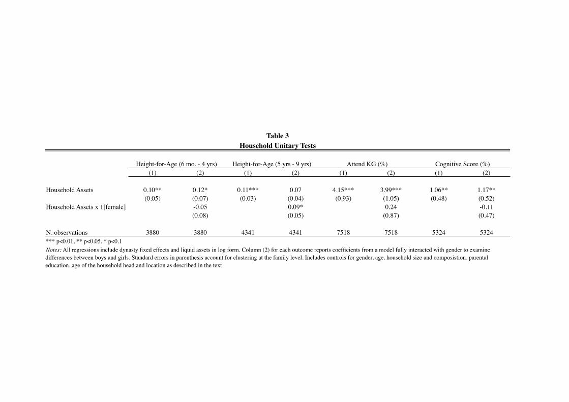
(1) (2) (1) (2) (1) (2) (1) (2)

Household Assets 0.10** 0.12* 0.11*** 0.07 4.15*** 3.99*** 1.06** 1.17**(0.05) (0.07) (0.03) (0.04) (0.93) (1.05) (0.48) (0.52)

Household Assets x 1[female] -0.05 0.09* 0.24 -0.11(0.08) (0.05) (0.87) (0.47)

N. observations 3880 3880 4341 4341 7518 7518 5324 5324*** p<0.01, ** p<0.05, * p<0.1

Table 3

Notes: All regressions include dynasty fixed effects and liquid assets in log form. Column (2) for each outcome reports coefficients from a model fully interacted with gender to examine differences between boys and girls. Standard errors in parenthesis account for clustering at the family level. Includes controls for gender, age, household size and composistion, parental education, age of the household head and location as described in the text.

Household Unitary Tests

Height-for-Age (6 mo. - 4 yrs) Height-for-Age (5 yrs - 9 yrs) Attend KG (%) Cognitive Score (%)

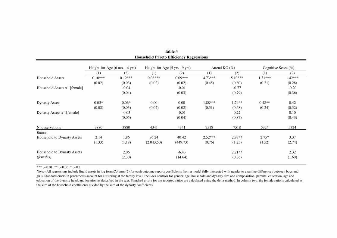
(1) (2) (1) (2) (1) (2) (1) (2)Household Assets 0.10*** 0.12*** 0.08*** 0.09*** 4.73*** 5.10*** 1.31*** 1.42***

(0.02) (0.03) (0.02) (0.02) (0.45) (0.60) (0.21) (0.28)Household Assets x 1[female] -0.04 -0.01 -0.77 -0.20

(0.04) (0.03) (0.79) (0.36)

Dynasty Assets 0.05* 0.06* 0.00 0.00 1.88*** 1.74** 0.48** 0.42(0.02) (0.03) (0.02) (0.02) (0.51) (0.68) (0.24) (0.32)

Dynasty Assets x 1[female] -0.03 -0.01 0.22 0.10(0.05) (0.04) (0.87) (0.43)

N. observations 3880 3880 4341 4341 7518 7518 5324 5324RatiosHousehold to Dynasty Assets 2.14 1.86 96.24 40.42 2.52*** 2.93** 2.75* 3.37

(1.33) (1.18) (2,043.50) (449.73) (0.76) (1.25) (1.52) (2.74)

2.06 -6.43 2.21** 2.32(2.30) (14.64) (0.86) (1.60)

*** p<0.01, ** p<0.05, * p<0.1

Table 4

Notes: All regressions include liquid assets in log form.Column (2) for each outcome reports coefficients from a model fully interacted with gender to examine differences between boys and girls. Standard errors in parenthesis account for clustering at the family level. Includes controls for gender, age, household and dynasty size and composistion, parental education, age and education of the dynasty head, and location as described in the text. Standard errors for the reported ratios are calculated using the delta method. In column two, the female ratio is calculated as the sum of the household coefficients divided by the sum of the dynasty coefficients

Household to Dynasty Assets (females)

Household Pareto Efficiency Regressions

Height-for-Age (6 mo. - 4 yrs) Height-for-Age (5 yrs - 9 yrs) Attend KG (%) Cognitive Score (%)

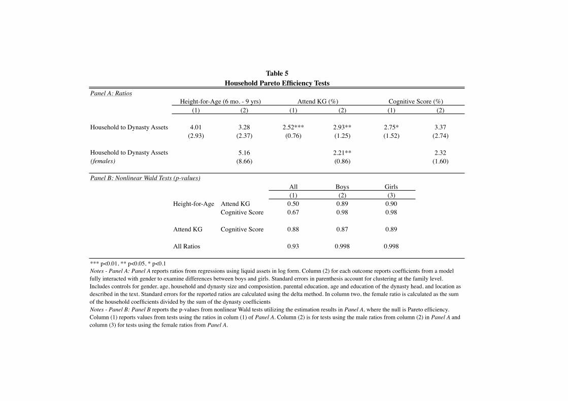
Panel A: Ratios

(1) (2) (1) (2) (1) (2)

Household to Dynasty Assets 4.01 3.28 2.52*** 2.93** 2.75* 3.37(2.93) (2.37) (0.76) (1.25) (1.52) (2.74)

5.16 2.21** 2.32(8.66) (0.86) (1.60)

All Boys Girls(1) (2) (3)

Height-for-Age Attend KG 0.50 0.89 0.90Cognitive Score 0.67 0.98 0.98

Attend KG Cognitive Score 0.88 0.87 0.89

All Ratios 0.93 0.998 0.998

*** p<0.01, ** p<0.05, * p<0.1Notes - Panel A: Panel A reports ratios from regressions using liquid assets in log form. Column (2) for each outcome reports coefficients from a model fully interacted with gender to examine differences between boys and girls. Standard errors in parenthesis account for clustering at the family level. Includes controls for gender, age, household and dynasty size and composistion, parental education, age and education of the dynasty head, and location as described in the text. Standard errors for the reported ratios are calculated using the delta method. In column two, the female ratio is calculated as the sum of the household coefficients divided by the sum of the dynasty coefficientsNotes - Panel B: Panel B reports the p-values from nonlinear Wald tests utilizing the estimation results in Panel A, where the null is Pareto efficiency. Column (1) reports values from tests using the ratios in colum (1) of Panel A. Column (2) is for tests using the male ratios from column (2) in Panel A and column (3) for tests using the female ratios from Panel A.

Table 5Household Pareto Efficiency Tests

Panel B: Nonlinear Wald Tests (p-values)

Height-for-Age (6 mo. - 9 yrs) Attend KG (%) Cognitive Score (%)

Household to Dynasty Assets (females)

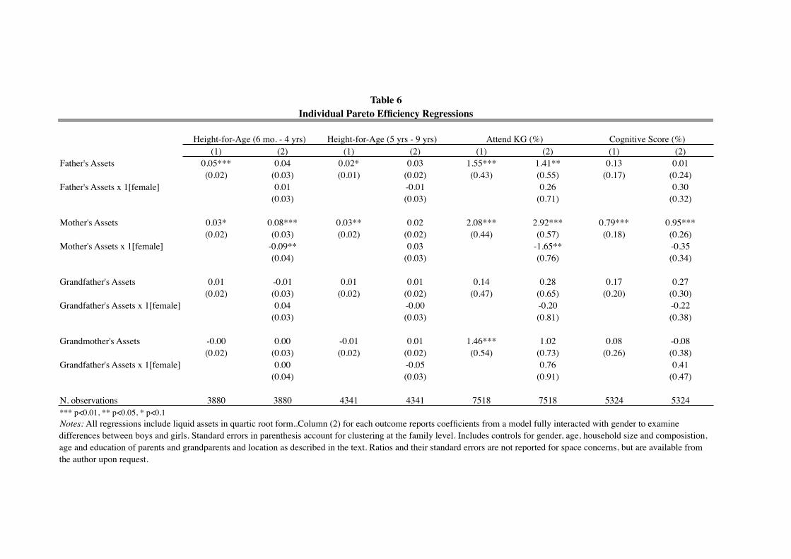
(1) (2) (1) (2) (1) (2) (1) (2)Father's Assets 0.05*** 0.04 0.02* 0.03 1.55*** 1.41** 0.13 0.01

(0.02) (0.03) (0.01) (0.02) (0.43) (0.55) (0.17) (0.24)Father's Assets x 1[female] 0.01 -0.01 0.26 0.30

(0.03) (0.03) (0.71) (0.32)

Mother's Assets 0.03* 0.08*** 0.03** 0.02 2.08*** 2.92*** 0.79*** 0.95***(0.02) (0.03) (0.02) (0.02) (0.44) (0.57) (0.18) (0.26)

Mother's Assets x 1[female] -0.09** 0.03 -1.65** -0.35(0.04) (0.03) (0.76) (0.34)

Grandfather's Assets 0.01 -0.01 0.01 0.01 0.14 0.28 0.17 0.27(0.02) (0.03) (0.02) (0.02) (0.47) (0.65) (0.20) (0.30)

Grandfather's Assets x 1[female] 0.04 -0.00 -0.20 -0.22(0.03) (0.03) (0.81) (0.38)

Grandmother's Assets -0.00 0.00 -0.01 0.01 1.46*** 1.02 0.08 -0.08(0.02) (0.03) (0.02) (0.02) (0.54) (0.73) (0.26) (0.38)

Grandfather's Assets x 1[female] 0.00 -0.05 0.76 0.41(0.04) (0.03) (0.91) (0.47)

N. observations 3880 3880 4341 4341 7518 7518 5324 5324*** p<0.01, ** p<0.05, * p<0.1

Table 6

Notes: All regressions include liquid assets in quartic root form..Column (2) for each outcome reports coefficients from a model fully interacted with gender to examine differences between boys and girls. Standard errors in parenthesis account for clustering at the family level. Includes controls for gender, age, household size and composistion, age and education of parents and grandparents and location as described in the text. Ratios and their standard errors are not reported for space concerns, but are available from the author upon request.

Individual Pareto Efficiency Regressions

Height-for-Age (6 mo. - 4 yrs) Height-for-Age (5 yrs - 9 yrs) Attend KG (%) Cognitive Score (%)

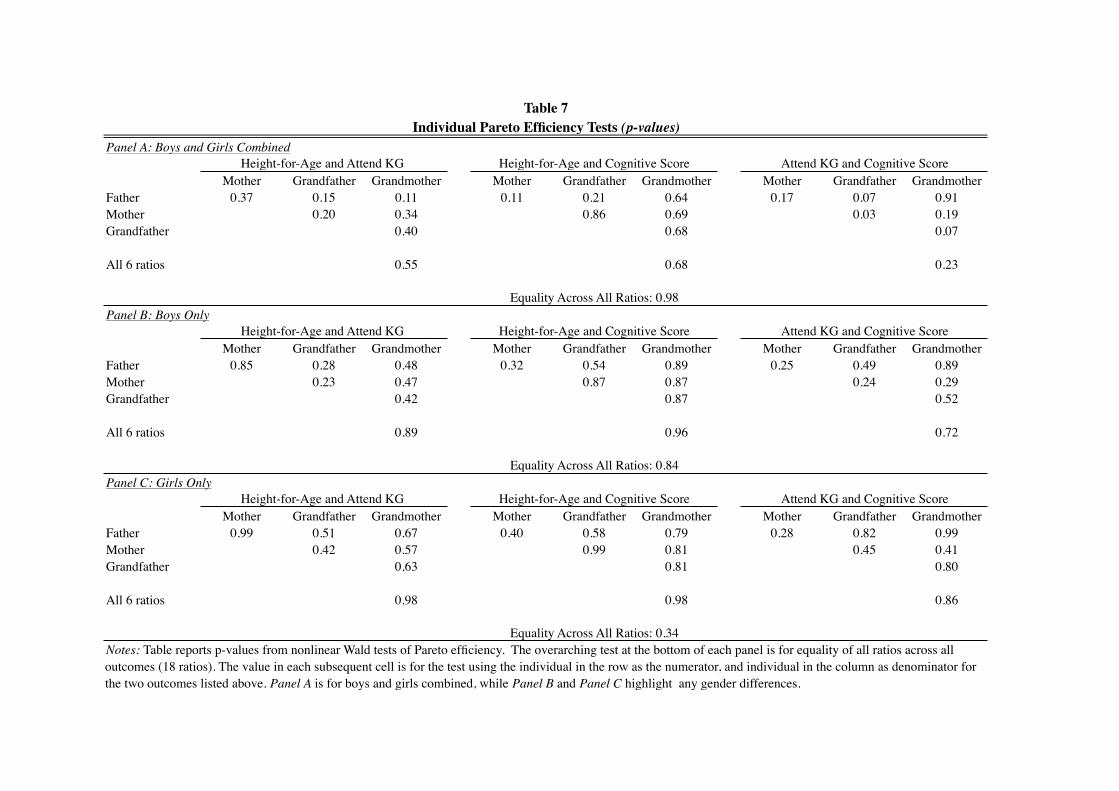
Panel A: Boys and Girls Combined

Mother Grandfather Grandmother Mother Grandfather Grandmother Mother Grandfather GrandmotherFather 0.37 0.15 0.11 0.11 0.21 0.64 0.17 0.07 0.91Mother 0.20 0.34 0.86 0.69 0.03 0.19Grandfather 0.40 0.68 0.07

All 6 ratios 0.55 0.68 0.23

Panel B: Boys Only

Mother Grandfather Grandmother Mother Grandfather Grandmother Mother Grandfather GrandmotherFather 0.85 0.28 0.48 0.32 0.54 0.89 0.25 0.49 0.89Mother 0.23 0.47 0.87 0.87 0.24 0.29Grandfather 0.42 0.87 0.52

All 6 ratios 0.89 0.96 0.72

Panel C: Girls Only

Mother Grandfather Grandmother Mother Grandfather Grandmother Mother Grandfather GrandmotherFather 0.99 0.51 0.67 0.40 0.58 0.79 0.28 0.82 0.99Mother 0.42 0.57 0.99 0.81 0.45 0.41Grandfather 0.63 0.81 0.80

All 6 ratios 0.98 0.98 0.86

Table 7

Height-for-Age and Attend KG

Notes: Table reports p-values from nonlinear Wald tests of Pareto efficiency. The overarching test at the bottom of each panel is for equality of all ratios across all outcomes (18 ratios). The value in each subsequent cell is for the test using the individual in the row as the numerator, and individual in the column as denominator for the two outcomes listed above. Panel A is for boys and girls combined, while Panel B and Panel C highlight any gender differences.

Height-for-Age and Attend KG Height-for-Age and Cognitive Score Attend KG and Cognitive Score

Individual Pareto Efficiency Tests (p-values)

Height-for-Age and Attend KG Height-for-Age and Cognitive Score Attend KG and Cognitive Score

Equality Across All Ratios: 0.98

Equality Across All Ratios: 0.84

Equality Across All Ratios: 0.34

Height-for-Age and Cognitive Score Attend KG and Cognitive Score

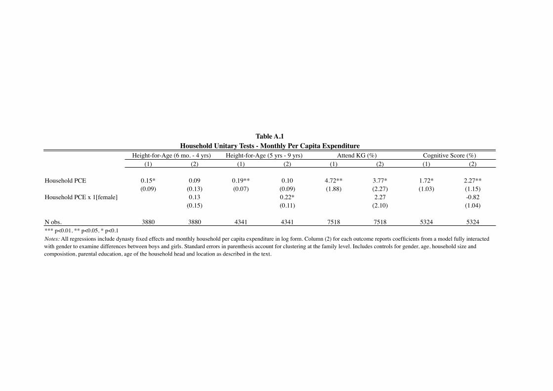
(1) (2) (1) (2) (1) (2) (1) (2)

Household PCE 0.15* 0.09 0.19** 0.10 4.72** 3.77* 1.72* 2.27**(0.09) (0.13) (0.07) (0.09) (1.88) (2.27) (1.03) (1.15)

Household PCE x 1[female] 0.13 0.22* 2.27 -0.82(0.15) (0.11) (2.10) (1.04)

N obs. 3880 3880 4341 4341 7518 7518 5324 5324*** p<0.01, ** p<0.05, * p<0.1Notes: All regressions include dynasty fixed effects and monthly household per capita expenditure in log form. Column (2) for each outcome reports coefficients from a model fully interacted with gender to examine differences between boys and girls. Standard errors in parenthesis account for clustering at the family level. Includes controls for gender, age, household size and composistion, parental education, age of the household head and location as described in the text.

Table A.1

Height-for-Age (6 mo. - 4 yrs) Height-for-Age (5 yrs - 9 yrs) Attend KG (%) Cognitive Score (%)Household Unitary Tests - Monthly Per Capita Expenditure

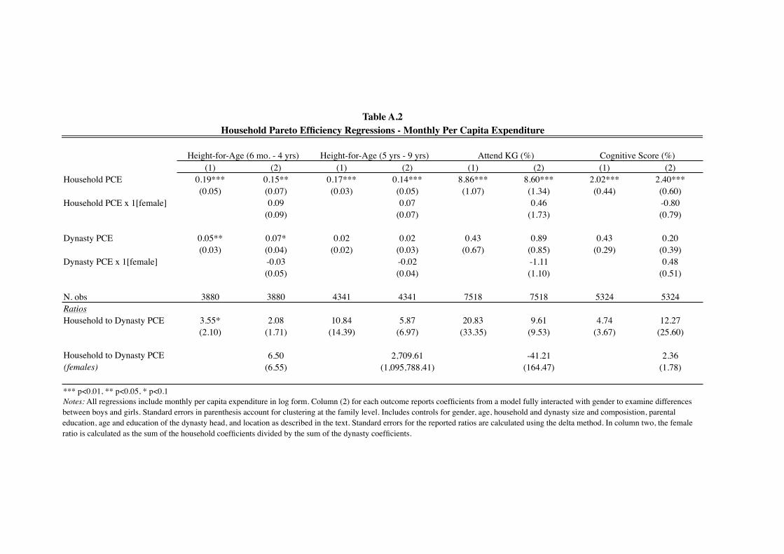
(1) (2) (1) (2) (1) (2) (1) (2)Household PCE 0.19*** 0.15** 0.17*** 0.14*** 8.86*** 8.60*** 2.02*** 2.40***

(0.05) (0.07) (0.03) (0.05) (1.07) (1.34) (0.44) (0.60)Household PCE x 1[female] 0.09 0.07 0.46 -0.80

(0.09) (0.07) (1.73) (0.79)

Dynasty PCE 0.05** 0.07* 0.02 0.02 0.43 0.89 0.43 0.20(0.03) (0.04) (0.02) (0.03) (0.67) (0.85) (0.29) (0.39)

Dynasty PCE x 1[female] -0.03 -0.02 -1.11 0.48(0.05) (0.04) (1.10) (0.51)

N. obs 3880 3880 4341 4341 7518 7518 5324 5324RatiosHousehold to Dynasty PCE 3.55* 2.08 10.84 5.87 20.83 9.61 4.74 12.27

(2.10) (1.71) (14.39) (6.97) (33.35) (9.53) (3.67) (25.60)

6.50 2,709.61 -41.21 2.36(6.55) (1,095,788.41) (164.47) (1.78)

*** p<0.01, ** p<0.05, * p<0.1Notes: All regressions include monthly per capita expenditure in log form. Column (2) for each outcome reports coefficients from a model fully interacted with gender to examine differences between boys and girls. Standard errors in parenthesis account for clustering at the family level. Includes controls for gender, age, household and dynasty size and composistion, parental education, age and education of the dynasty head, and location as described in the text. Standard errors for the reported ratios are calculated using the delta method. In column two, the female ratio is calculated as the sum of the household coefficients divided by the sum of the dynasty coefficients.

Table A.2Household Pareto Efficiency Regressions - Monthly Per Capita Expenditure

Household to Dynasty PCE (females)

Height-for-Age (6 mo. - 4 yrs) Height-for-Age (5 yrs - 9 yrs) Attend KG (%) Cognitive Score (%)

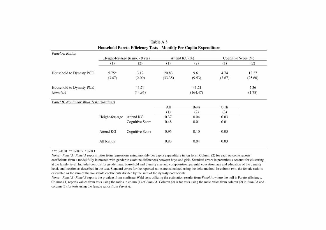
Panel A: Ratios

(1) (2) (1) (2) (1) (2)

Household to Dynasty PCE 5.75* 3.12 20.83 9.61 4.74 12.27(3.47) (2.09) (33.35) (9.53) (3.67) (25.60)

11.74 -41.21 2.36(14.95) (164.47) (1.78)

All Boys Girls(1) (2) (3)

Height-for-Age Attend KG 0.37 0.04 0.03Cognitive Score 0.48 0.01 0.01

Attend KG Cognitive Score 0.95 0.10 0.05

All Ratios 0.83 0.04 0.03

*** p<0.01, ** p<0.05, * p<0.1

Household to Dynasty PCE (females)

Panel B: Nonlinear Wald Tests (p-values)

Notes - Panel A: Panel A reports ratios from regressions using monthly per capita expenditure in log form. Column (2) for each outcome reports coefficients from a model fully interacted with gender to examine differences between boys and girls. Standard errors in parenthesis account for clustering at the family level. Includes controls for gender, age, household and dynasty size and composistion, parental education, age and education of the dynasty head, and location as described in the text. Standard errors for the reported ratios are calculated using the delta method. In column two, the female ratio is calculated as the sum of the household coefficients divided by the sum of the dynasty coefficients.Notes - Panel B: Panel B reports the p-values from nonlinear Wald tests utilizing the estimation results from Panel A, where the null is Pareto efficiency. Column (1) reports values from tests using the ratios in colum (1) of Panel A. Column (2) is for tests using the male ratios from column (2) in Panel A and column (3) for tests using the female ratios from Panel A.

Table A.3Household Pareto Efficiency Tests - Monthly Per Capita Expenditure

Height-for-Age (6 mo. - 9 yrs) Attend KG (%) Cognitive Score (%)