Extended vector-tensor theories

Rampei Kimura, Atsushi Naruko, Daisuke Yoshida

Department of Physics, Tokyo Institute of Technology, 2-12-1 Ookayama, Meguro-ku, Tokyo 152-8551, Japan

E-mails: rampei@th.phys.titech.ac.jp, naruko@th.phys.titech.ac.jp,yoshida@th.phys.titech.ac.jp

Abstract. Recently, several extensions of massive vector theory in curved space-time have beenproposed in many literatures. In this paper, we consider the most general vector-tensor theoriesthat contain up to two derivatives with respect to metric and vector field. By imposing a degeneracycondition of the Lagrangian in the context of ADM decomposition of space-time to eliminate anunwanted mode, we construct a new class of massive vector theories where five degrees of freedomcan propagate, corresponding to three for massive vector modes and two for massless tensor modes.We find that the generalized Proca and the beyond generalized Proca theories up to the quarticLagrangian, which should be included in this formulation, are degenerate theories even in curvedspace-time. Finally, introducing new metric and vector field transformations, we investigate theproperties of thus obtained theories under such transformations.

arX

iv:1

608.

0706

6v4

[gr

-qc]

20

Apr

201

7

Contents

1 Introduction 1

2 Vector-tensor theories 32.1 The action 32.2 3+1 Decomposition 52.3 Block-diagonalized kinetic matrix 72.4 Metric and vector field transformations 9

3 Degenerate vector-tensor theories 93.1 Degeneracy condition 103.2 Generalized Proca theory 123.3 Beyond generalized Proca theory 133.4 Case A : General theories with α1 + α2 = 0 14

3.4.1 Relation with the (beyond) generalized Proca theories 173.5 Case B : General theories with α1 + α2 6= 0 20

4 Summary and discussion 23

A Details of transformations 25A.1 Conformal and disformal metric transformations and vector field redefinition 25A.2 Transformation of the Einstein-Maxwell theory 27A.3 Transformation of the Generalized Proca theory 28A.4 Transformation to Simple Frame 30

A.4.1 f = 1 frame 30A.4.2 f = 1 and β = 0 frame 30

B Determinants in Case A and B 31

C Case C : General theories with f = 0 36

1 Introduction

The late-time accelerating expansion of the universe [1, 2] is one of the most challenging and intriguingproblems in cosmology. As a candidate for explaining the accelerated expansion of the universe,modified gravity theories have been intensively studied in recent years (see for reviews e.g. [3, 4]).The most simplest way to modify Einstein’s gravity could be to introduce an additional scalar degreeof freedom in general relativity, called scalar-tensor theories of gravity. Although a number of thescalar-tensor theories have been so far proposed in various contexts, an interesting scalar-tensortheory would be the galileon theory [5], whose Lagrangian contains higher, that is at least second,derivatives of the scalar field. Surprisingly, its special structure prevents third or higher derivativeterms from appearing in the equation of motion for a scalar field, which in general leads to a ghostmode, hence it is free of Ostrogradski instability. The galileon field have been discovered in thecontext of an effective field theory of modified gravity theories. For example, the cubic galileon

– 1 –

field is originated from a brane bending mode in the decoupling limit [6, 7] of the Dvali-Gabadadze-Poratti brane-world scenario [8], and the quartic and quintic galileon interactions as well as thecubic galileon are subsequently found in the decoupling limit of the de Rham-Gabadadze-Tolleymassive gravity [9, 10]. The galileon self-interactions can be generalized in a curved space-timerequiring that equations of motion for both scalar field and gravity remain at most second-orderdifferential equations [11], and the most general scalar-tensor theory, whose equations of motioncontains up to the second derivatives of the fields, is called the Horndeski theory [12–14]. However,it was pointed out that one can further generalize these constructions without a ghost mode byallowing higher order derivatives in the equations of motion, dubbed as the beyond Horndeski or theGLPV theory [15]. Furthermore, the recent works in [16] showed that more general constructions ofscalar-tensor theories is possible as long as they satisfy a degeneracy condition to eliminate the would-be Ostrogradski mode. Such degenerate theories have been also investigated based on Hamiltonianformulation in [17, 18], confirming the presence of an additional primary constraint which is necessaryto eliminate the Ostrogradski mode. The detailed classification and the cosmological applications ofeach extended scalar-tensor theory have been investigated in [19] and [20], respectively.

Another attempt to modify general relativity is to introduce an Abelian vector field. In massivegravity theory, a massive graviton carries five degrees of freedom, and one can separate out thetensor part and the vector part by introducing the Stuckelberg field, hµν → hµν + ∂µAν + ∂νAµ.The vector Lagrangian in the decoupling limit of massive gravity does not only contain the standardMaxwell Lagrangian but also includes fully nonlinear corrections [21, 22]. Motivated by this fact,vector-tensor theory is still a natural extension as an effective theory of gravity. In the pioneer work[23], the authors showed no-go theorem which states that the galileon-like terms are not allowed ina flat space-time under the assumption of U(1) invariance, while in a curved space-time the vectorHorndeski term [24] is allowed. However, once we relax the condition of U(1) invariance, the vectorfield is no longer massless, and a finite number of interactions can be found. This extended theoryof the massive vector field is called the generalized Proca (GP) theory [25] which consists of sixinteraction terms in a flat space-time. The higher order Lagrangian can be similarly constructed inthe same manner [26], however it identically vanishes by virtue of the Newton’s identities as in theflat galileon [27]. Covariantization procedure of the GP theory in a flat space-time can be similarlydone as in the case of the generalized galileon. Furthermore, one can construct ”beyond” type vectorderivative interactions (beyond GP theory) as in the beyond Horndeski theory [28]. Summarizingthese results, the vector-tensor theory investigated so far is described by the following action,

SVT =

∫d4x√−g

[6∑

n=2

Ln +

6∑m=4

L(B)m

], (1.1)

where the GP interactions Ln are given by

L2 = G2(Y, F 2, F F , (AF )2), (1.2a)

L3 = G3(Y )∇µAµ, (1.2b)

L4 = G4(Y )R− 2G4,Y [(∇µAµ)2 −∇µAν∇νAµ], (1.2c)

L5 = G5(Y )Gµν∇µAν +1

3G5,Y [(∇µAµ)3 − 3∇µAµ∇ρAσ∇σAρ + 2∇ρAσ∇γAρ∇σAγ ] (1.2d)

−G5(Y )FαµF βµ∇αAβ, (1.2e)

L6 = G6(Y )Lµναβ∇µAν∇αAβ −G6,Y FαβFµν∇αAµ∇βAν , (1.2f)

– 2 –

and the beyond GP interactions L(B)m are given by

L(B)4 = G

(B)4 (Y ) εµνρσεαβγσAµAα∇νAβ∇ρAγ , (1.3a)

L(B)5 = G

(B)5 (Y ) εµνρσεαβγδAµAα∇νAβ∇ρAγ∇σAδ + G

(B)5 εµνρσεαβγδAµAα∇νAρ∇βAγ∇σAδ, (1.3b)

L(B)6 = G

(B)6 (Y ) εµνρσεαβγδ∇µAν∇αAβ∇ρAγ∇σAδ. (1.3c)

Here, G3,4,5,6, G(B)4,5,6, G5, and G

(B)5 are arbitrary functions of the Proca mass term Y = AµA

µ, G2

are arbitrary functions of Y , the Maxwell kinetic term F 2 = FµνFµν , FF = FµνF

µν , and (AF )2 =AµAνF α

µ Fνα, where Fµν = ∇µAν−∇νAµ, andGi,Y stands for ∂Gi/∂Y . The dual strength tensor and

the double dual Riemann tensor are defined as Fµν = εµναβFαβ/2 and Lµναβ = εµνρσεαβγσRρσγδ/4.These Lagrangians with the replacement, Aµ → ∂µφ, coincide with the Horndeski and the beyondHorndeski Lagrangians which are invariant under a shift symmetry, φ→ φ + constant. This Horn-deski structure guarantees that this φ field does not contain higher derivatives, meaning the absenceof the Ostrogradsky ghost in the situation such that the vector field is simply replaced by the gradientof the φ field. One should note that U(1) gauge invariant Lagrangian can be found when the arbi-trary functions G3, G4, G5, and G6 in the GP theory are set to be constant and G2 = G2(F 2, F F )and G5 = 0. The remaining Lagrangians, after integration by parts, are those associated with G2,G4, and G6, and the massless vector field is described by the arbitrary function of the Maxwellkinetic term and FF , the Einstein-Hilbert term, and the vector Horndeski [24]. The cosmologicalapplications of the GP and beyond GP theories have been recently studied in [29–31], and a Higgsmechanism and black hole solutions for these theories are discussed in [32, 33] and [34], respectively.

Now we want to address a question : “Is this the most general vector-tensor theory withoutintroducing an extra (would-be ghostly) degree of freedom ? ”. The answer is probably no. As canbe seen in the case of scalar-tensor theories, one can further extend vector-tensor theories with adegeneracy condition in the kinetic matrix which can kill the would-be dangerous mode. To thisend, in the present paper we investigate the most general degenerate vector-tensor theories up toquadratic order in the first derivatives of the vector field.

This paper is organized as follows. In section 2, we introduce vector-tensor theories whoseLagrangian contain up to two derivatives acting on the vector and metric tensor fields. Then, wederive a kinetic matrix and a degeneracy condition by the use of 3 + 1 decomposition withoutgauge fixing. In section 3, we investigate the most general theories which satisfy the degeneracycondition and classify all the possible cases. We also link the GP and the beyond GP theorieswith our new theories utilizing conformal and disformal transformations as well as a vector fieldredefinition. Section 4 is devoted to the conclusion. Details on metric and vector field transformationsare summarized in appendix A. The explicit expressions of determinant of kinetic matrices in the casesA and B are collected in appendix B. Finally, the analysis of the case C, where the Einstein-Hilbertterm is absent, is performed in appendix C.

2 Vector-tensor theories

2.1 The action

We consider a class of vector-tensor theories, whose generic action contains up to two derivativeswith respect to gµν and Aµ :

S[gµν , Aµ] ≡∫d4x√−g

(f R+ Cµνρσ∇µAν ∇ρAσ +G3∇µAµ +G2

), (2.1)

– 3 –

where R is the Ricci scalar and ∇µ represents a covariant derivative with respect to the space-timemetric, gµν . The tensor Cµνρσ depends on gµν , Aµ and εµνρσ, which is defined as 1

Cµνρσ = α1gµ(ρgσ)ν + α2g

µνgρσ +1

2α3(AµAνgρσ +AρAσgµν)

+1

2α4(AµA(ρgσ)ν +AνA(ρgσ)µ) + α5A

µAνAρAσ + α6gµ[ρgσ]ν

+1

2α7(AµA[ρgσ]ν −AνA[ρgσ]µ) +

1

4α8(AµAρgνσ −AνAσgµρ) +

1

2α9ε

µνρσ. (2.2)

Here, we introduced arbitrary functions of Y = AµAµ such as f = f(Y ), αi = αi(Y ), G3 = G3(Y )

and G2 = G2(Y ). With our best knowledge, it will be the first time in the literature that the termwith α8 is taken into account, which induces the cross term of Fµν and Sµν as seen in (2.5). We notethat another possible term like AµAν∇µAν can be absorbed into G3 after integration by parts :

G3,Y (Y )AµAν∇µAν = −1

2G3(Y )∇µAµ +

1

2∇µ(G3(Y )Aµ

), (2.3)

where the subscript , Y represents a derivative with respect to Y . Furthermore, one might notice thatthe non-minimal coupling of the vector field to gravity, G4(Y )GµνA

µAν , should be systematicallyintroduced since it carries two derivatives. However, this term can be similarly absorbed into Cµνρσ

term up to a total derivative, thanks to the identity, (∇µ∇ν −∇ν∇µ)Aρ = RµνρσAσ.

For later convenience, let us rewrite the vector self-interactions in terms of the symmetric andanti-symmetric parts of ∇µAν ,

Sµν = ∇µAν +∇νAµ, Fµν = ∇µAν −∇νAµ, (2.4)

and we then have

4Cµνρσ∇µAν∇ρAσ = α1SµνSµν + α2(Sµ

µ)2 + α3AµAνSµνSρ

ρ

+α4AµAνSµρSν

ρ + α5(AµAνSµν)2 + α6FµνFµν

+α7AµAνFµρFν

ρ + α8AµAνFµ

ρSνρ + α9FµνFµν . (2.5)

One might think that it is possible to add terms related to the dual of Fµν such as AµAνFµρFνρ and

AµAνFµρSνρ. The first term can be rewritten as

AµAνFµρFνρ =

1

4Y FµνF

µν , (2.6)

where we have used the identity FµρFνρ = (FαβFαβ/4) δµν , derived in [35, 36]. Thus, this term is

already included in (2.5). Furthermore, it is easy to show that the second term AµAνFµρSνρ can be

rewritten as

G9,Y (Y )AµAνFµρSνρ =

1

2G9(Y )FµνF

µν + G9,Y (Y )AµAνFµρFνρ −∇µ

(G9(Y )AνF

µν)

=

(1

2G9(Y ) +

1

4Y G9,Y (Y )

)FµνF

µν −∇µ(G9(Y )AνF

µν). (2.7)

1The symmetrization and anti-symmetrization are normalized by

T (µν) =1

2(Tµν + T νµ) , T [µν] =

1

2(Tµν − T νµ) .

– 4 –

where we have used (2.6) in the second equality. Therefore, all the possible terms related to the dualof Fµν can be totally absorbed into α9FµνF

µν . In light of these facts, Cµνρσ in (2.2) is the mostgeneral form, which is composed by Aµ, gµν , and εµνρσ.

In the GP and the beyond GP theories, the α6 and α7 terms in (2.2) was classified to L2

as an analogue of the k-essence term [37, 38] in scalar field theories because these terms do notcarry the dangerous time-derivative of the time-component, A0. However, in more general set-up,these arbitrary functions are also responsible for satisfying a degeneracy condition, and hence thosecontributions in addition to the one from α8 must be properly taken into account as we will discussthis issue in the next section.

Before the end of this subsection, we discuss the connection with scalar-tensor theories. Asdiscussed in [25], a subclass of the GP theory can be obtained from the shift-symmetric Horndeskitheory, which enjoys a symmetry of the action under φ → φ + const. , just by replacing ∇µφ withAµ. However, our theory of the vector field cannot be obtained from any kinds of scalar field theories(even the ones recently formulated in [17, 18]) via such direct replacement of the fields. Since theindices of ∇µ∇νφ is symmetric, only the symmetric parts of Cµνρσ in (2.1) and (2.2) can survive inthe case of scalar field :

Cµνρσ(∇µ∇νφ)(∇ρ∇σφ) = C(µ ν) (ρ σ)(∇µ∇νφ)(∇ρ∇σφ). (2.8)

As a matter of fact, even in the case of the GP theory, G5 term in (1.2e) and G6 term in (1.2f)cannot be also obtained from the shift-symmetric Horndeski theory since they are identically zero[25–27]. To put it another way, since the anti-symmetric part of Cµνρσ is automatically dropped offin the theory of the scalar field, we cannot explore a whole class of vector field theories where thoseanti-symmetric parts can play an important role.

2.2 3+1 Decomposition

In order to write down a degeneracy condition for the kinetic matrix, we need to extract the timederivative component of the action (2.1). A convenient way to do this without gauge fixing is 3 + 1decomposition. To the end, we assume space-time manifold is foliated by spacelike hypersurfaces Σt.Let us define normal vector nµ of each hypersurface Σt, which satisfies nµnµ = −1. The inducedmetric on Σt, γµν , are defined by

γµν = gµν + nµnν . (2.9)

Any covariant tensor fields can be decomposed by this induced metric and the normal vector. Forexample, Aµ can be decomposed as

Aµ = −nµA∗ + Aµ, (2.10)

where we define

A∗ := nµAµ, (2.11a)

Aµ := γµνAν . (2.11b)

The derivative of the normal vector can also be decomposed into the extrinsic curvature Kµν andacceleration vector aµ,

∇µnν = −nµaν +Kµν , (2.12)

– 5 –

where the extrinsic curvature and the acceleration vector are defined by

aµ := nν∇νnµ, (2.13a)

Kµν := γµργν

σ∇ρnσ. (2.13b)

Then, the first derivative of the vector field reads

∇µAν = nµnν(A∗ − aρAρ) + nµ(− ˙Aν +Kν

ρAρ + aνA∗)

+(KµρAρ −DµA∗)nν +DµAν −KµνA∗, (2.14)

where Dµ represents a covariant derivative with respect to the spatial metric, γµν and a dot representsthe Lie derivative along nµ:

A∗ = £nA∗ = nµ∇µA∗, (2.15a)

˙Aµ = £nAµ = nν∇νAµ + Aν∇µnν . (2.15b)

The kinetic part of the Lagrangian (2.1) can be expressed in terms of A∗, Aµ, γµν , and Kµν as

Lkin = AA2∗ + 2BiA∗

˙Aµ + 2CµνA∗Kµν +Dµν ˙

Aµ˙Aν + 2Eµνρ ˙

AµKνρ + FµνρσKµνKρσ, (2.16)

with

A =α1 + α2 − (α3 + α4)A2∗ + α5A

4∗, (2.17a)

Bµ =− 1

4AµA∗(−2α3 − 2α4 + α8 + 4α5A

2∗), (2.17b)

Cµν =1

2A∗(−α3 − 2α4 + 2α5A

2∗)A

µAν +1

2A∗(4fY + 2α2 − α3A

2∗)γ

µν , (2.17c)

Dµν =− 1

4(α4 + α7 − α8 − 4α5A

2∗)A

µAν +1

4(−2α1 − 2α6 +A2

∗(α4 + α7 + α8))γµν , (2.17d)

Eµνρ =α1γµ(νAρ) +

1

2(−4fY + α3A

2∗)A

µγνρ +1

4AµAνAρ(2α4 − α8 − 4α5A

2∗), (2.17e)

Fµνρσ =(f + α1A2∗)γ

µ(ργσ)ν + (−f + α2A2∗)γ

µνγρσ +1

2(4fY − α3A

2∗)(A

µAνγρσ + AρAσγµν)

− α1(AµA(ργσ)ν + AνA(ργσ)µ) + 2(−α4 + α5A2∗)A

µAνAρAσ, (2.17f)

where we have also used

R = (3)R+KµνKµν −K2 − 2∇µ(aµ −Knµ) , (2.18)

and (3)R stands for the three-dimensional Ricci scalar composed by the spatial metric, γµν , andK = γµνKµν . Note that the kinetic Lagrangian does not depend on α9. This is because theterm α9FµνF

µν only contains up to the first Lie derivative of Aµ, i.e., α9 can be freely chosen inconstructing degenerate theories.

– 6 –

2.3 Block-diagonalized kinetic matrix

The kinetic Lagrangian we obtained in the previous subsection is still involved to analyze the struc-ture of vector-tensor theories. We would like to simplify this kinetic Lagrangian by changing thebasis to the one, which can (even partially) diagonalize the kinetic matrix based on the irreduciblerepresentation. Following the pioneering work [17], we introduce two unit spatial vectors uµ and vµ,which satisfy

uµuµ = vµvµ = 1, uµvµ = vµAµ = Aµuµ = 0 , (2.19)

and

nµuµ = nµvµ = 0. (2.20)

The vector Aµ can be normalized by Aµ/|A| where we define the inner product of the spatial com-

ponent as A2 = AµAµ and |A| represents

√A2. Then, we can build orthogonal bases of the three

dimensional vector space on Σt, Vaµ (a runs from 1 to 3) as

V 1µ =

Aµ

|A|, V 2

µ = uµ, V 3µ = vµ, (2.21)

which satisfy V aµ V

bµ = δab and γµν = δabVaµV b

ν . By using these unit vectors, one can construct

the following 6 independent symmetric matrices U Iµν (I runs from 1 to 6),

U1µν =

1

A2AµAν , U2

µν =1√2

(γµν − U1µν), U3

µν =1√2

(uµuν − vµvν),

U4µν =

1√2

(uµvν + uνvµ), U5µν =

1√2 |A|

(uµAν + uνAµ), U6µν =

1√2 |A|

(vµAν + vνAµ), (2.22)

which satisfy U IµνUJµν = δIJ . Since U Iµν span the space of symmetric tensors on Σt, these tensors

satisfy the relations γµ(ργνσ) = δIJU

IµνUJρσ. Then, we can decompose˙Aµ and Kµν along these

vector and tensor bases :

˙Aµ = Aa V

aµ , Kµν = KI U

Iµν . (2.23)

Each coefficient such as Aa and KI can be obtained by projecting˙Aµ and Kµν onto those bases,

Aa = V aµ ˙Aµ and KI = U IµνKµν . In terms of V a

µ and U Iµν , one can construct the scalar, vector, andtensor quantities which transform as scalar, vector, and tensor respectively under a rotation aroundthe axis, Aµ. For example, the contraction of any vector field with V 1

µ extract the scalar component

in the vector field while that with V 2,3µ yields the vector components.

Now the kinetic Lagrangian is rewritten as

Lkin = AA2∗ + 2BA∗A1 + 2A∗(C1K1 + C2K2) +D1A

21 +D2(A2

2 + A23)

+2A1(E1K1 + E2K2) + 2E3(A2K5 + A3K6)

+F1K21 + F2K

22 + 2F3K1K2 + F4(K2

3 +K24 ) + F5(K2

5 +K26 ), (2.24)

– 7 –

where the coefficients are given by

A = α1 + α2 − (α3 + α4)A2∗ + α5A

4∗, (2.25a)

B =1

4(2α3 + 2α4 − α8 − 4α5A∗)A∗|A|, (2.25b)

C1 =1

2

(4fY + 2α2 − α3A

2∗ − (α3 + 2α4)A2 + 2α5A

2∗A

2)A∗, (2.25c)

C2 =1√2

(4fY + 2α2 − α3A2∗)A∗, (2.25d)

D1 = −1

4

(2(α1 + α6) + (α4 + α7 − α8)A2 − (α4 + α7 + α8)A2

∗ − 4α5A2∗A

2), (2.25e)

D2 = −1

4

(2(α1 + α6)− (α4 + α7 + α8)A2

∗

), (2.25f)

E1 = −1

4|A|(

8fY − 4α1 − (2α4 − α8)A2 − 2α3A2∗ + 4α5A

2∗A

2), (2.25g)

E2 = − 1√2

(4fY − α3A2∗)|A|, (2.25h)

E3 =1√2α1|A|, (2.25i)

F1 = (α1 + α2)A2∗ + (4fY − 2α1)A2 − α3A

2∗A

2 − α4A4 + α5A

2∗A

4, (2.25j)

F2 = −f + (α1 + 2α2)A2∗, (2.25k)

F3 = − 1√2

(2f − 4fY A

2 − 2α2A2∗ + α3A

2∗A

2), (2.25l)

F4 = f + α1A2∗, (2.25m)

F5 = f + α1A2∗ − α1A

2. (2.25n)

We can further rewrite this kinetic Lagrangian by using two 4× 4 matrices and 2× 2 matrix,

Lkin =(mT mT

1 mT2

)M 0 00 M1 00 0 M2

mm1

m2

, (2.26)

where we defined the component column matrices m = A∗, A1,K1,K2, m1 = A2, A3,K5,K6,and m2 = K3,K4, and a matrix with a superscript T represents the transposed matrix. Thematrices M, M1, and M2 describe the kinetic matrices of the scalar, vector and tensor sectors,respectively whose explicit forms are given by

M =

A B C1 C2

B D1 E1 E2

C1 E1 F1 F3

C2 E2 F3 F2

, M1 =

D2 0 E3 00 D2 0 E3

E3 0 F5 00 E3 0 F5

, M2 =

(F4 00 F4

). (2.27)

Interestingly, the scalar, vector, and tensor sectors are never mixed due to the different transformationproperty, and they can be treated independently as can be seen in (2.26). Note that this is true onlyif the Lagrangians contains up to two derivatives with respect to space-time, i.e., the kinetic part ofthe Lagrangians is strictly quadratic.

– 8 –

In the construction of degenerate vector-tensor theories, we need to remove the extra degree offreedom in the scalar sector, which typically contains the Ostrogradsky ghost. This is exactly thesame situation as in the scalar-tensor theories, however the crucial difference in here is the presenceof the A1 components in the kinetic matrix M. Due to this additional component in the kineticmatrix, the degeneracy condition in the scalar-tensor theories, which removes the ghostly degree offreedom, will no longer satisfy the degeneracy condition in the vector-tensor theories in general.

2.4 Metric and vector field transformations

Metric and vector field transformations are potent tools to investigate the basic properties of gravi-tational theories. We here consider new types of metric transformations by invoking a vector field2.As a natural extension of the metric transformation with a scalar field, the new transformation isgiven by

gµν → gµν = Ω(Y ) gµν + Γ(Y )AµAν . (2.28)

Here, we introduced the conformal factor Ω and the disformal factor Γ which are functions of Ywhile they can be functions of φ and X = gµν∇µφ∇νφ in the case of scalar field. Although it maybe possible to include derivatives of the vector field in the disformal/conformal factors as in the caseof the scalar field, we only focus on the most general derivative-independent metric transformation(2.28) in the present paper for simplicity.

Moreover, let us introduce a field redefinition of the vector field by

Aµ → Aµ = Υ(Y )Aµ, (2.29)

where Υ is called a rescaling factor, which is a function of Y . Apparently, there is no analog of thiskind of the field redefinition in scalar field theories since this is not a simple redefinition of φ norX. Throughout this paper, we assume that the metric transformations (2.28) and the vector fieldredefinition (2.29) satisfy Ω > 0 and Υ 6= 0. We also assume that the metrics in both frames haveLorentzian signatures, det gµν < 0 and det gµν < 0, which translate into Ω + Y Γ > 0 from (A.5).

After straightforward but tedious computation, one can show that the action (2.1) is invariantunder the metric transformation (2.28) and vector field redefinition (2.29) by redefining arbitraryfunctions such as f and αi, that is, the form of the action reduces to the same form under these trans-formations. The result is quite reasonable since the number of derivatives is preserved under thesetransformations. All the technical details associated with the metric and vector field transformationsare summarized in appendix A.

3 Degenerate vector-tensor theories

In this section, we derive a degeneracy condition of the kinetic matrix M in (2.27) to eliminate thedangerous mode, and then we focus on the classification of extended vector-tensor theories based onthe degeneracy condition.

2A disformal transformation of the vector field in a Minkowski background, ηµν → ηµν + Γ(Y )AµAν , has firstintroduced in [27].

– 9 –

3.1 Degeneracy condition

We wish to find degenerate theories where the matrixM has at least one zero eigenvalue, which canbe checked in the eigenvalue equation of M,

det (M− λI) = detM+ y1λ+ y2λ2 + y3λ

3 + λ4 = 0, (3.1)

where I is the identity matrix and λ is the eigenvalue. The necessary condition to remove theunwanted degree of freedom is given by detM = 0, which implies the existence of a primary constraint(see for the detail in the context of classical mechanics [39]). Then, the appropriate number ofconstraints should exist depending on whether this system is a first or second class, and vector-tensor theories, which satisfies detM = 0, have at most five degrees of freedom. Furthermore, it ispossible that M has two or more zero eigenvalues when y1 (or subsequently y2 and y3) is zero. Onetherefore needs to carefully check the number of zero eigenvalues to confirm the number of degreesof freedom. As we will see, in order to have y1 = 0, we additionally need to tune the arbitraryfunctions. In the present paper, we mainly focus on the case in which only one of the eigenvalues iszero, i.e., detM = 0 but y1,2,3 6= 0 as a generalization of the Proca theory.

We now want to write down detM in the power series of A∗. Since f and αi are functionsof Y , we can re-express the matrix elements in terms of Y and A∗ by replacing A by its definition,Y = −A2

∗+A2. The determinant of this matrix is formally given by the following form which containsup to A4

∗,

detM = D0(Y ) +D1(Y )A2∗ +D2(Y )A4

∗. (3.2)

Here, D0(Y ) is given by

D0(Y ) =1

16(α1 + α2)Q(f, α1, α2, α4, α8, β), (3.3)

where

Q(f, α1, α2, α4, α8, β) = 8f2(

2α1 − β + (α4 − α8)Y)

+ 32Y 2f2Y

(2α1 − β + (α4 + α8)Y

)+Y f

(8α1β + 16fY (2α1 + β + α4Y )− 192f2

Y + α28Y

2 + 4α4βY), (3.4)

and we have introduced a convenient variable :

β = −2α6 − α7Y. (3.5)

Since α6 and α7 always appear in this combination in the matrix M, the determinant is solelydetermined by β, not α6 and α7 independently. On the other hand, M1 and M2 individuallydepend on both α6 and α7.

Then, D1 is given by

D1(Y ) = W1 α28 +W2 α8 +W3, (3.6)

where we defined

W1 =1

8(α1 + α2)Y 2f +

1

16Y (f − α1Y )

(2f + (α1 + 3α2)Y

), (3.7a)

W2 =1

4(α1 + α2)

(4(4Y 2f2

Y − f2) + Y f(α1 + α2 + Y (α3 + α4) + α5Y

2))

− 1

16Y (2α2 + 4fY + α3Y )

(16α1Y fY + f(2α2 − 12fY + α3Y )

), (3.7b)

– 10 –

W3 =1

4(α1 + α2)

(α5

(α4Y

3f + Y f (−8f + 2α1Y − βY ))

+ α24Y

2f

+ α4Y(4βf + Y

(−3α1β + 4α1fY + 16f2

Y

))+ 2 (α1 − 2fY ) (Y (4 (α1 + β) fY − 3α1β)− 2f (α1 − β − 6fY ))

)+

1

2α1Y

(α1β (2α1 + α4Y )− 2fY

(4α1β + 4fY (α4Y − β) + α3α4Y

2 − α3βY + 2α1α3Y))

+1

16f(

8fY(−12α2

1 + 6fY (2α1 − β + α4Y ) + 2α1 (3β + (5α3 + α4)Y ) + α3Y (α4Y − β))

+ β(−12α2

1 + α23Y

2 − 4 (3α3 + 4α4)α1Y)

+ (2α1 − α3Y ) (6α1 + α3Y ) (2α1 + α4Y ))

+1

2(α3 + α4) f2 (−2α1 + β + α3Y ) . (3.7c)

Finally, while the expression of D2 itself is quite involved, a linear combination of D0, D1, and D2

takes a rather simple form as

D1(Y )− Y D2(Y ) = − 1

16Y(f − α1Y )

(2α1 + (α4 + α8)Y − β

)×[

4(α1 + α2 + (α3 + α4)Y + α5Y

2)(

2f + (α1 + 3α2)Y)

− 3Y (2α2 + 4fY + α3Y )2

]+D0(Y )

Y. (3.8)

Then, the degeneracy condition can translate into the following conditions,

D0(Y ) = D1(Y ) = D2(Y ) = 0. (3.9)

In the subsection 3.4 and 3.5, we will use D1(Y ) − Y D2(Y ) = 0 instead of D2(Y ) = 0 as anindependent condition in classifying degenerate vector-tensor theories since the expression is muchsimpler than D2(Y ) itself. We immediately notice that (3.3) has two branches: α1 + α2 = 0 andQ(f, α1, α2, α4, α8, β) = 0 with α1 + α2 6= 0. The former case corresponds to a broader class ofthe GP and the beyond GP theories since α1 + α2 = 0 is also satisfied in both theories, while thelatter case is a completely new class of vector-tensor theories. In order to count the total degreesof freedom, we also need to check the degeneracy/non-degeneracy of the matrices M1 and M2 toexamine the presence of further additional primary constraint(s). For example, the determinant ofM2 is zero only if f = α1 = 0 since it is solely determined by F4 = f + α1A

2∗, which corresponds to

no tensor modes, and there is no gravitational wave in this case. We also summarize the expressionof M1 in appendix B.

The detailed analysis below proceeds as follows. We first take a look at the special two cases,which correspond to the GP and the beyond GP theories in the next two subsections. Then, weinvestigate the general case and find all possible branches, which satisfy the degeneracy condition(3.9). In subsection 3.4, we focus on the case α1 + α2 = 0 denoted as the case A, and then thecase α1 + α2 6= 0 with Q(f, α1, α2, α4, α8, β) = 0, denoted as the case B, will be investigated in thesubsection 3.5. We here only consider f 6= 0 case, and the f = 0 case are summarized in appendixC. We also summarize all results of detM1 and y1 for each case in appendix B. The schematic figureof the classification are shown in figure 1.

– 11 –

3.2 Generalized Proca theory

The action of the GP theory [25] up to the quartic Lagrangian can be rewritten in terms of Sµν andFµν as

SGP =

∫d4x√−g(L2 + L3 + L4), (3.10)

with

L2 = G2 + α6FµνFµν + α7A

µAνFµρFρν + α9FµνF

µν , (3.11a)

L3 = G3∇µAµ, (3.11b)

and

L4 = G4R− 2G4,Y

((∇µAµ)2 −∇µAν∇νAµ

)= G4R−

1

2G4,Y

(FµνF

µν + SµµSνν − SµνSµν

), (3.11c)

where K,α6, α7, α9, G3 and G4 are functions of Y . The second term in the last line can be removedby the redefinition of α6. This Lagrangian is found when

f = G4, α1 = −α2 = 2G4,Y , α3 = α4 = α5 = α8 = 0. (3.12)

Here, α6, α7, and α9 will be still chosen as free parameters. In this case, the kinetic matrix (2.27)can be written as

M =

0 0 0 0

0(β − 4fY )

40 − 2

√2fY |A|

0 0 0 −√

2(f − 2Y fY )

0 ∗ ∗ − 2A2∗fY − f

, (3.13)

where asterisks represent symmetric components. One observes that all the first row and column arezero, leading to detM = 0. This ensures that the GP theory is the degenerate theory, and one canfreely choose β and α9 as stated in the above.

One also needs to check the other determinants, and they are in fact non-zero in general,

detM1 =1

16Y 2

[2Y(f(2fY + α6)− 2fY Y α6

)+(

8f2Y Y + f(2α6 + β)− 2fY Y (2α6 + β)

)A2

∗

]2

,

(3.14a)

y1 = −1

2(4fY − β)(f − 2fY Y )2, (3.14b)

y2 = −2(f − 2fY Y )2 + 4fY (f − 2fY Y )− 1

4f(12fY + β)− 1

2fY (12fY + β)A2

∗, (3.14c)

y3 = f + fY −β

4+ 2fYA

2∗. (3.14d)

– 12 –

Note that if β = 4fY or f = c√|Y | with a constant c, y1 vanishes. In the former case, y2 and y3

does not vanish for any arbitrary functions with f 6= 0. Furthermore, the vector sector degenerateonce we impose the additional condition α6 = −2ffY /(f − 2fY Y ). On the other hand, in thelatter case f = c

√|Y |, y2 can also vanish if we make an additional choice of the arbitrary function,

β = −6c√|Y |/Y . In this case, y3 6= 0. Theories with the above parameter choices might imply the

existence of an additional primary constraint, which can eliminate one of the three vector degrees offreedom.

3.3 Beyond generalized Proca theory

The beyond GP theory [28] up to the quartic Lagrangian can be written as

SBGP = SGP +

∫d4x√−gL(B)

4 , (3.15)

with

L(B)4 = G

(B)4 εµνρσεαβγσAµAα∇νAβ∇ρAγ

=1

4G

(B)4

(2AαAβF γ

α Fβγ −AαAαFβγF βγ − 2AαAβS γα Sβγ

+AαAαSβγS

βγ + 2AαAβSαβSγγ −AαAαSββSγγ

). (3.16)

Note that the first and second terms can be absorbed into L2. One can construct another interactionfrom the beyond Horndeski theory via replacements such as ∇µφ→ Aµ

3,

L(B)4,2 = G

(B)4 εµνρσεαβγσAµAα∇νAρ∇βAγ

=1

2G

(B)4

(2AαAβF γ

α Fβγ −AαAαFβγF βγ). (3.17)

But one will immediately notice that this is already included in L2. Therefore, the beyond GP theoryis given by

f = G4, α1 = −α2 = 2G4,Y +G(B)4 Y, α3 = −α4 = 2G

(B)4 , α5 = α8 = 0. (3.18)

Again, α6, α7, and α9 can be still chosen as free parameters. In this case, the kinetic matrix isexplicitly written as

M =

0 0 0α4A∗A

2

√2

0(β − 4fY )

20 −(α4A

2∗ + 4fY )|A|√

2

0 0 04Y fY − 2f + α4(A4

∗ + 2A2∗Y )√

2

∗ ∗ ∗ 1

2A2

∗(α4Y − 4fY )− f

, (3.19)

3 In fact, three types of the quartic beyond GP Lagrangian can be constructed by using the replacement ∇µφ→ Aµ,

which are (3.16), (3.17), and G(beyond)4 εµνρσεαβγσAµAαSνβFργ . However, the last interaction is trivially zero, and this

is the reason why the term with α8 is missing in [27].

– 13 –

where asterisks again represent symmetric components. Since the first row is linearly dependent onthe third row, the determinant of the kinetic matrix vanishes, and hence the beyond GP theory isalso the degenerate theory. Then, detM1, y1, y2, and y3 are given by

detM1 =1

64Y 2

[2Y(

2fα6 + (f − α6Y )(4fY − α4Y ))

+(−2(f + 2Y fY )α4Y + 16Y f2

Y + (2f − 4Y fY + α4Y2)(2α6 + β)

)A2

∗

]2,

(3.20a)

y1 =1

8(β − 4fY )

[4(f − 2fY Y )2 − Y α4(8f − 16fY Y − α4Y )A2

∗

− 2α4(2f − 4fY Y − α4Y − 2α4Y2)A4

∗ + (1 + 4Y )α24A

6∗ + α2

4A8∗

], (3.20b)

y2 = −2f2 − β

4f + ffY (1 + 8Y )− 8f2

Y Y (1 + Y )

+1

8

[32Y α4f − Y α4(4Y α4 − β)− 48f2

Y − 4fY

(Y (9 + 16Y )α4 + β

)]A2

∗

− 1

2α4

(Y (3 + 4Y )α4 − 4f + 8fY (1 + Y )

)A4

∗ − (1 + 2Y )α24A

6∗ −

α24

2A8

∗, (3.20c)

y3 = f + fY −β

4+(

2fY −Y α4

2

)A2

∗. (3.20d)

One might notice that y1 can be zero only if β = 4fY with non-zero α4, and the vector sectoragain degenerate when α6 = f(α4Y −4fY )/(2f+(α4Y −4fY )Y ). As in the previous case, this choicemight eliminate an additional degrees of freedom in vector modes, however this should be carefullychecked in Hamiltonian analysis, which will not be discussed in the present paper. As investigated inappendix A, the beyond GP theory can be obtained from the GP theory by performing a disformaltransformation, and the disformal factor Γ(Y ) therefore corresponds to the additional parameter

G(B)4 (Y ) in the beyond GP theory. On the other hand, the theory obtained from the beyond GP

theory by performing a disformal transformation still belongs to the beyond GP theory up to theredefinition of arbitrary functions. However, once we perform a conformal transformation and/orvector field redefinition from the GP theory, the resultant theory no longer belongs to the beyondGP theory.

3.4 Case A : General theories with α1 + α2 = 0

In this subsection, we consider the case α1 +α2 = 0, which is required to satisfy the first degeneracycondition (3.9), and here assume f 6= 0. The special case where the Einstein-Hilbert term is absent isinvestigated in appendix C. First, let us consider (3.8), which is also required to vanish. Substitutingα1 = −α2 in (3.8), we obtain

0 = − 1

16(f + α2Y )

((α4 + α8)Y − 2α2 − β

)×[

8(α3 + α4 + α5Y )(f + α2Y )− 3(2α2 + 4fY + α3Y )2

]. (3.21)

– 14 –

Extended vector-tensor

theories

D0(Y ) = 0

D1(Y ) = 0Case A1 (3.24)

Case A2 (3.25)

Case A3 (3.27)

Case A4 (3.31)

Case B1 (3.51)

Case B2 (3.53)

Case B3 (3.54)

Case B5 (3.58)

Case B4 (3.56)

Case B6 (3.60)

Case B

↵1 + ↵2 6= 0

f 6= 0

Case A

↵1 + ↵2 = 0f 6= 0

Case C

f = 0

f, ↵4, ↵5, ↵6, ↵7, ↵8

f, ↵3, ↵5, ↵6, ↵7, ↵8

f, ↵4, ↵5, ↵6, ↵7, ↵8

f, ↵2, ↵3, ↵5, ↵6, ↵7

f, ↵2, ↵3, ↵6, ↵7, ↵8

f, ↵1, ↵2, ↵3, ↵6, ↵7

f, ↵1, ↵2, ↵3, ↵6, ↵7

f, ↵2, ↵3, ↵5, ↵6, ↵7

f, ↵2, ↵3, ↵6, ↵7, ↵8

f, ↵1, ↵6, ↵7, ↵8

Free functions

D1(Y ) Y D2(Y ) = 0

Figure 1. Classification of extended vector-tensor theories, which satisfies the degeneracy condition (3.9).The theories with f 6= 0 is divided into the case A and the case B on the basis of the conditions, α1 + α2 = 0or α1 + α2 6= 0. On the other hand, the theory with f = 0, the case C, automatically satisfies the conditionD0(Y ) = 0. The further branches are obtained from the other conditions D1(Y )−Y D2(Y ) = 0 and D1(Y ) = 0in all cases. The detailed classification of the case C in appendix C is omitted, for simplicity. In each individualcase, the example of the set of free functions is shown on the right side. Note that in the case A4 the freefunctions f and α2,3,5 is required to satisfy the condition W 2

2 − 4W1W3 ≥ 0.

This has three branches, which are given by

α2 = − fY

or α2 =(α4 + α8)Y − β

2

or α4 =3(2α2 + 4fY + α3Y )2

8(f + α2Y )− (α3 + α5Y ). (3.22)

Here, we assumed f + α2Y 6= 0 in the last branch of (3.22). Substituting the first branch of (3.22)into D1(Y ), we get

0 = D1(Y ) =f

16Y 3

(Y (4fY + α3Y )− 2f

)2(6f + Y β − (α4 + α8)Y 2

). (3.23)

Then, we have two solutions in the first branch of (3.22),Case A1 :

α1 = −α2 =f

Y, α3 =

2(f − 2fY Y )

Y 2, (3.24)

– 15 –

Case A2 :

α1 = −α2 =f

Y, α4 =

6f + Y β

Y 2− α8. (3.25)

In both cases, each matrix element of M is not zero. The case A1 corresponds to the ”class Ib” inthe scalar-tensor theories, which was found in [19]. This is because the degeneracy condition (3.24)is completely independent on β and α8, that is, only the symmetric part of ∇µAν in the Lagrangian(2.1) plays a role to satisfy the degeneracy condition (3.9). As confirmed in [19], the vector sectorfurther degenerate in the ”class Ib”. On the other hand, in our case, the vector sector does notstill degenerate since we now have two additional vector components, A2 and A3, in the matrixM1,which are apparently absent in the scalar-tensor theories.

Substituting the second branch of (3.22) into D1(Y ), we get

0 = D1(Y ) =1

32Y[(

(α4 + α8)Y − β)

(8fY − 2β + α8Y )− 2(2α3 + 2α4 + α8)f]2. (3.26)

One can easily solve this for α3, and we have only one solution,Case A3 :

α1 = −α2 = −(α4 + α8)Y − β2

,

α3 =

((α4 + α8)Y − β

)(−2β + 8fY + α8Y )− 2(2α4 + α8)f

4f. (3.27)

D1(Y ) in the third branch of (3.22) can be written as the power series in α8 as in Eq. (3.6),

0 = D1(Y ) = W1(f, α2)α28 +W2(f, α2, α3)α8 +W3(f, α2, α3, α5, β) , (3.28)

where W1, W2, and W3 are given by

W1(f, α2) =1

8Y (f + α2Y )2, (3.29a)

W2(f, α2, α3) =1

16Y (2α2 + 4fY + α3Y )

[4fY (4α2Y + 3f)− f(2α2 + α3Y )

], (3.29b)

W3(f, α2, α3, α5, β) = P1(f, α2, α3, β)α5 + P2(f, α2, α3, β)(2α2 + 4fY + α3Y ), (3.29c)

with

P1(f, α2, α3, β) = − 1

16Y

[8α2Y

2(α2β + 2α3Y fY + 8f2Y ) + 8f2(2α2 + β + α3Y )

+ Y f(

16α2β + 12α22 + 8fY (α3Y − 2α2)

+ 48f2Y − α2

3Y2 + 4α2α3Y

)], (3.30a)

– 16 –

P2(f, α2, α3, β) =1

128Y (f + α2Y )−1

×[

32α3f2(2α2 + β + α3Y )

+ f(−24α3

2 − 4fY (8α2β + 36α22 − 3α2

3Y2 + 44α3α2Y )

+ 48f2Y (2α2 + 5α3Y ) + 576f3

Y − 3α33Y

3 + 14α2α3Y (4β + α3Y )

+ 4α22(7α3Y − 4β)

)+ 8α2Y

(α2β(−2α2 − 4fY + 3α3Y )

+ 2fY(24fY (α2 + α3Y ) + 48f2

Y + α3Y (3α3Y − 2α2)))]

. (3.30b)

Therefore, one can solve this for α84 and we have

Case A4 :

α1 = −α2 , α4 =3(2α2 + 4fY + α3Y )2

8(f + α2Y )− α3 − α5Y , α8 =

−W2 ±√W 2

2 − 4W1W3

2W1.v (3.31)

Since α8 has to be a real function, we require W 22 − 4W1W3 ≥ 0, and f and α2,3,5 have to be chosen

so that this condition is satisfied. In the above analysis, we have assumed f +α2Y 6= 0 and the casef + α2Y = 0 is included in the first branch, namely the case A1 or A2.

3.4.1 Relation with the (beyond) generalized Proca theories

Here, we discuss the relation of the case A with the GP and beyond GP theories. As we will seebelow, a certain subclass of these theories are included in the cases A1, A2 and A3. However, as isclear from the number of the arbitrary functions, new theories are also included in these cases. Onthe other hand, all the remaining theories of the GP and beyond GP theories belong to the case A4.More interestingly, all the rest of the case A4 is nothing but the one that can be obtained throughthe transformations (2.28) and (2.29) of the GP and beyond GP theories. This is compatible withthe fact that the number of arbitrary functions in the case A4 is equal to that in the GP theory plusthree transformation parameters, that is, the conformal, the disformal and the rescaling factors5.However, new theories also exist in the case A4 as we see below.

First, we make clear the relation of the cases A1, A2 and A3 with the GP and beyond GPtheories. Comparing the parameters in the case A1 (3.24) with those in the GP theory (3.12), thecase A1 includes the special case of the GP theory when

f = G4 = c√|Y | , α4 = α5 = α8 = 0 , (3.32)

where c represents an arbitrary constant. On the other hand, the special case of the beyond GPtheory can be included in the case A1 when

f = G4 , α4 = −α3 , α5 = α8 = 0 , G(B)4 =

G4 − 2Y G4,Y

Y 2. (3.33)

4Although the quadratic equation in α8 (3.28) has two solutions, we unified two branches into one case in ourclassification because +(−) branch is connected with −(+) branch via a metric transformation (2.28) and a fieldredefinition (2.29).

5In the case of the beyond GP theory, the transformation parameters are only the conformal and the rescalingfactors since its action is invariant under the disformal transformation up to the redefinition of arbitrary functions.However, the number of arbitrary functions in the case A4 is equal to the number of arbitrary functions (G4, G

(B)4 , α6

and α7) plus two transformation parameters as in the case of the GP theory.

– 17 –

As for the case A2, one notice that a subclass of the GP theory is included when

f = G4 = c√|Y | , α3 = α5 = α8 = 0 , β = −6G4

Y= −6c

√|Y |Y

. (3.34)

Now the arbitrary function β must be also tuned when f 6= 0. A subclass of the beyond GP theorybelongs to this case if

f = G4 , α3 = −α4 , α5 = α8 = 0 , G(B)4 =

G4 − 2Y G4,Y

Y 2, β = 4

Y G4,Y − 2G4

Y. (3.35)

In the case A3, the GP theory is included when

f = G4 , α4 = α5 = α8 = 0 , β = 4G4,Y , (3.36)

and the beyond GP theory is included when

f = G4 , α4 = −2G(B)4 , α5 = α8 = 0 , β = 4G4,Y . (3.37)

The parameter choices f = c√|Y | in (3.32) and (3.34) and β = 4G4,Y in (3.36) and (3.37) correspond

to the cases that the scalar sector is further degenerate, y1 = 0.As we have seen, a subclass of the GP and beyond GP theories with particular arbitrary

functions are included in the cases A1, A2 and A3, but there must exist new theories in thosecases according to the number of the arbitrary functions. For example in the case A1, we havearbitrary functions, f, α4, α5, α6, α7, α86 while the GP theory with G4 ∝

√|Y | and an arbitrary

β belongs to this case. Given the fact that we only have three transformations factors (2.28) and(2.29), apparently we cannot explore the whole parameter space through the transformation of theabove specific GP theory. Then, we conclude that new degenerate vector-tensor theories must existin the case A1 as well as the cases A2 and A3, which cannot be obtained from any known theoriesthrough transformations. Furthermore, we confirmed that the theories after the transformations stillsatisfy the same degeneracy conditions of the original frame, and different branches based on ourclassification are never mixed by any kinds of the transformations that we have introduced in thepresent paper.

Let us move to the case A4. The degeneracy conditions (3.31) is satisfied with the parametersof the GP (3.12) and the beyond GP (3.18) theory except for special cases (3.32)-(3.37), which arerelated with the cases A1, A2 and A3. Therefore, one concludes that both the GP and the beyond GPtheories are included in the case A4 in general. The degeneracy conditions (3.31) are strictly preservedby the metric transformation (2.28) and the field redefinition (2.29). Thus, any theory transformedfrom the GP theory, including the beyond GP theory, belongs to the case A4. Moreover, since thereare six arbitrary functions f, α2, α3, α5, α6, α7 in the case A4, one would expect that the GP theorycan be mapped from the case A4. To see this, we want to re-express six parameters, namely threearbitrary functions in the GP theory, G4, α6, α7, and three transformation parameters, Ω,Γ,Υ,in terms of six functions in the case A4, f, α2, α3, α5, α6, α7. Using (A.24), we get the first orderdifferential equations for Ω and Γ as

ΩY =4fY + 2α2 + Y α3

4(f + α2Y )Ω, (3.38a)

ΓY = 2Γf + α2(ΓY + Ω)

f + α2Y

ΥY

Υ+

2α2(α2 + 2fY )− α3(2f + α2Y )

4(f + α2Y )2Ω . (3.38b)

6 One can choose different free functions, for example, α1 instead of f in the case A1 (3.24). In this case, the set offree functions is given by α1, α4, α5, α6, α7, α8, however the number of free functions is indeed unchanged.

– 18 –

GP & Beyond GP theoryCase A1

Case A2

Case A3

Case A4

(non-invertible)

(invertible)

Figure 2. The relation between the (beyond) GP theories and the case A through the transformations(2.28) and (2.29). The shaded regions correspond to the new theories of massive vector field in curved space-time, which satisfies the degeneracy condition (3.9). The arrow with the straight line represents invertibletransformation, and the dashed arrow represents non-invertible transformation.

Here, we have used the condition of the case A4, f + Y α2 6= 0. On the other hand, Υ is determinedby the following first order differential equation,

Z1

(ΥY

Υ

)2

+ 2Y Z2

(ΥY

Υ

)+ Z2 = 0, (3.39)

where we defined

Z1 = (f + Y α2)

[8(f + Y α2)(Y 2α5 − β − 2α2 − Y α3)

+Y (2α2 + 4fY + α3Y )(

10α2 − 3(4fY + α3Y ))], (3.40)

Z2 = 8α5(f + Y α2)2 + (2α2 + 4fY + α3Y )(

2α2(α2 + 2fY )− α3(4f + 3α2Y )). (3.41)

One can easily solve the equation for Υ, and we get

ΥY

Υ=

−Y Z2 ±

√Z2(Y 2Z2 − Z1)

Z1(Z1 6= 0),

− 1

2Y(Z1 = 0 and Z2 6= 0).

(3.42)

Surprisingly, the expression inside the square root in the solution of ΥY /Υ, (3.42), is proportionalto the one in the solution of α8, (3.31), namely

Z2(Y 2Z2 − Z1) =256

Y 2(W 2

2 − 4W1W3), (3.43)

– 19 –

which is required to be positive in the case A4. Therefore, we do not have to impose any additionalconstraint for the parameters. Hence one can always relate G4, α6, α7,Ω,Γ,Υ and f, α2, α3, α5, α6, α7by using the integrated expression of (3.38a), (3.38b), and (3.42). In other words, the case A4 canbe always mapped to the GP theory. After solving those differential equations one can also expressthe remaining functions as

G4 =f√

Ω(Ω + Y Γ), (3.44a)

α6 =fΓ + Ωα6

Υ2√

Ω(Ω + Y Γ), (3.44b)

α7 =

√ΓY + Ω

Υ2Y Ω5/2 (Υ + YΥY ) 2

[4Y

ΥY

ΥΩ(

Γ2Y (f + α2Y ) + 2α2ΓY Ω + (α2 − α6)Ω2)

+ 2Y Ω2Y f(ΓY + Ω) + 2Y 2 Υ2

Y

Υ2Ω(

Γ2Y f + α2(ΓY + Ω)2 − α6Ω2)

+ Ω(

2α2(ΓY + Ω)2 + 2Y Γ(Γf + α6Ω))

+ Ω2(ΓY + Ω)(4fY + α7Y )− 4ΩΩY (ΓY + Ω)(2Y fY + f)

]. (3.44c)

In figure 2, we show the schematic figure of the relation between the (beyond) GP theories and thecase A via the transformations (2.28) and (2.29).

Before the end of this section, let us make a comment on the case with non-invertible transforma-tion. As studied in [40, 41], if the transformation is non-invertible, where the inverse transformationdoes not exist, the resultant theory has nothing to do with the original theory. The special casesin the case A4, which can be formally mapped from the GP theories through such non-invertibletransformations, have completely different properties from those in the corresponding GP theories.Such a case can be for example found when the parameters in the case A4 satisfy

f = Y , α3 =2α2

Y, α5 =

2α2

Y 2, (3.45)

Further careful study is necessary for such special cases. We will defer this interesting subject infuture work.

3.5 Case B : General theories with α1 + α2 6= 0

We now consider the second branch of (3.3) where Q(f, α1, α2, α4, α8, β) = 0 while α1 + α2 6= 0. Forsimplicity, we here set f = 1 and β = 0 throughout this subsection. As investigated in appendixA, these parameter choices can be realized after performing the conformal and the field redefinitionwithout loss of generality when f 6= 0, for completeness7. The case f = 0 is individually investigatedin appendix C.

As investigated in appendix A, the condition α1 + α2 6= 0 is preserved under any of conformaltransformation, disformal transformation (2.28), and vector field redefinition (2.29). In other words,

7Here, we implicitly assumed f > 0. One can in general consider f < 0, however it might lead to a wrong sign ofthe kinetic or gradient term of the tensor mode. Such an example can be found in the cosmological solution of the GPtheory in [29], and the tensor perturbation suffers from the ghost/gradient instabilities when f < 0. For f > 0, f canbe always set to be unity by a transformation with Ω > 0.

– 20 –

any theories in the case B are not connected to the GP and the beyond GP theories where α1+α2 = 0under the metric transformation and the vector field redefinition, and the case B can be thereforecategorized as the new class of theories.

After plugging f = 1 and fY = β = 0 into the second branch of (3.3), we have 8

Q = 8(

2α1 + Y (α4 − α8))

+ Y 3α28 = 0. (3.46)

In this case, we can solve this for α4, and we have

α4 = −2α1

Y+ α8 −

Y 2α28

8. (3.47)

Again, we consider (3.8) by utilizing f = 1, β = 0 and (3.47), which now reduces to

0 = − 1

256α8(1− α1Y )(16− α8Y

2)

×[(

2 + (α1 + 3α2)Y)(

8α8Y − α28Y

3 − 8(α1 − α2) + 8Y (α3 + Y α5))− 6Y (2α2 + α3Y )2

].

(3.48)

Then, we have five branches, which are given by

α8 = 0 or α1 =1

Yor α8 =

16

Y 2, or

α5 =α2

8Y

8− α8

Y+

8(α1 − α2) + 4(α21 + 2α1α2 − 2α3)Y − 4α1α3Y

2 + 3α23Y

3

4Y 2(

2 + (α1 + 3α2)Y) ,

or α2 = −2 + Y α1

3Y. (3.49)

Here, we assume that degeneracy conditions in the former branch of (3.49) is non-zero, for example,α8 6= 0 for the second branch α1 = 1/Y . The first branch of (3.49) gives

0 = D1(Y ) =(2α1 − Y α3)2

2Y− 2Y (α1 + α2)α5. (3.50)

We solve this for α5, and since α1 + α2 6= 0 we getCase B1 :

f = 1, β = 0, α4 = −2α1

Y, α5 =

(2α1 − Y α3)2

4Y 2(α1 + α2), α8 = 0. (3.51)

Now the second branch in (3.49) gives

0 = D1(Y ) =(α8Y

2 − 8)2(

2(2− Y 2α3)2 − Y 2α8(1 + Y α2)(8− α8Y2)− 8(1 + Y α2)α5Y

3)

256Y 3.(3.52)

8 It should be noted that, if α8 = 4/Y 2, the equation (3.46) completely coincides with the corresponding equationin the scalar-tensor theory.

– 21 –

Thus, we have two solutions,Case B2 :

f = 1, β = 0, α1 =1

Y, α4 = − 2

Y 2, α8 =

8

Y 2, (3.53)

Case B3 :

f = 1, β = 0, α1 =1

Y, α4 = − 2

Y 2+ α8 −

Y 2α28

8

α5 =(2− Y 2α3)2

4Y 3(1 + Y α2)− α8

Y+Y α2

8

8, (3.54)

where 1 + Y α2 6= 0 since α1 + α2 6= 0. The third branch in (3.49) gives

0 = D1(Y ) =1

2Y 3

[−4(α1 + α2)α5Y

4 + α23Y

4 + 12α1α3Y3

−4(7α21 + 16α1α2 + 4α3)Y 2 + 32(α1 + 4α2)Y + 64

]. (3.55)

Solving this for α5 we getCase B4 :

f = 1, β = 0, α4 = − 16

Y 2− 2α1

Y, α8 =

16

Y 2,

α5 =α2

3Y4 + 12α1α3Y

3 − 4(7α21 + 16α2α1 + 4α3)Y 2 + 32(α1 + 4α2)Y + 64

4Y 4(α1 + α2). (3.56)

The fourth branch in (3.49) gives

0 = D1(Y ) =(1− α1Y )

(2α1α8Y

2 + 8(2α2 + α3Y ) + Y (4 + 4Y α2 − Y 2α3)α8

)2

64Y((α1 + 3α2)Y + 2

) , (3.57)

where (α1 + 3α2)Y + 2 6= 0. The first solution, α1 = 1/Y , corresponds to the case B3 since theexpression of α5 in the forth branch (3.49) with α1 = 1/Y reduces the one in the case B (3.54).Therefore, we disregard this solution, and we getCase B5 :

f = 1, β = 0, α1 =−8(2α2 + Y α3)− Y (4 + 4Y α2 − Y 2α3)α8

2Y 2α8

α4 =4(1 + Y α2)

Y 2− α3 +

8(2α2 + Y α3)

Y 3α8+ α8 −

Y 2α28

8

α5 =−2 + Y 2α3

Y 3− 4(2α2 + Y α3)

Y 4α8− α8

Y+Y α2

8

8+

12(2α2 + Y α3)

Y 2(Y 2α8 − 8)(3.58)

Here, Y 2α8 − 8 6= 0 since (α1 + 3α2)Y + 2 6= 0. The last branch in (3.49), which corresponds to thecase (α1 + 3α2)Y + 2 = 0, provides the further condition from (3.8), so let us take a look at this first.It is now given by

0 = −α8(1− α1Y )(α8Y2 − 16)(−3α3Y

2 + 2α1Y + 4)2

384Y. (3.59)

– 22 –

The first solution α8 = 0 corresponds to the case B1, the second solution α1 = 1/Y corresponds tothe case B3, and the third solution α8 = 16/Y 2 corresponds to the case B4. Therefore, the remainingsolution isCase B6 :

f = 1, β = 0, α2 =−2− Y α1

3Y, α3 =

2(2 + Y α1)

3Y 2, α4 = −2α1

Y+ α8 −

Y 2α28

8,

α5 =2(Y α1 − 1)

3Y 3− α8

Y+Y α2

8

8. (3.60)

4 Summary and discussion

In this paper we propose a new class of extended vector-tensor theories, which carries at most fivedegrees of freedom, namely three for massive vector mode and two for massless tensor mode. Startingfrom the most general action for vector field which contains up to two derivatives with respect togµν and Aµ, we have imposed a degeneracy condition on the kinetic part of the action in order toeliminate the would-be Ostrogradski mode. We then have found a new class of degenerate vector-tensor theories denoted as the cases A, B, and C, which are not included in any known theoriessuch as the generalized Proca (GP) and the beyond generalized Proca theories. We also confirmedthat both the GP and beyond GP theories are the degenerate theories even in curved space-time asnaively expected in the previous works.

In the course of analysis, we have also extended metric transformations by incorporating a vectorfield. These transformations are characterized by the so-called conformal and disformal factors,which are functions of the vector field, more rigorously the contraction of vector field, Y = AµA

µ. Inaddition, we have introduced a field redefinition of the vector field, to which there is no analog in thescalar field language since this is not a mere redefinition of φ nor X. After checking that the actionis invariant under these transformations modulo redefinition of arbitrary functions, we confirmedthat classification of such degenerate theories is stable, that is, each case specified in the analysis isnever mixed and the same degeneracy condition still holds even after these transformations. Thisresult clarifies that our vector-tensor theories in the cases A1, A2 and A3, except for the specialexamples, and all of the case B are new theories, which cannot be obtained by any kinds of themetric transformations and the redefinition of vector field from the known vector-tensor theoriessuch as the GP and the beyond GP theories. We found that the remaining branch, the case A4,includes both the GP and the beyond GP theories up to the quartic Lagrangian. Furthermore, thetheory which is obtained from the (beyond) GP theory by the transformations (2.28) and (2.29)is also included in the case A4. Since the number of free functions of this branch is six, these sixfunctions can be regarded as the three free functions of the GP theory and the three free functionsof the transformations, as proved in section 3.4.1. While the theories which correspond to the non-shaded region in the case A4 in figure 2 can be mapped from the GP theory through invertibletransformations, and vice versa, specific theories which correspond to the shaded region in the caseA4 in figure 2 are related with the GP theory through non-invertible transformations. These specifictheories in the case A4 have nothing to do with the GP theory, and hence those theories should beregarded as new theories. In appendix C, we also classified the new theories with f = 0 denoted asthe case C, for completeness.

One of interesting directions of study is to seek for massless vector theories. Since the presenceof the degeneracy just promises one primary constraint, our vector-tensor theories also include the

– 23 –

theories which carry less than five degrees of freedom. One possibility to remove further degrees offreedom is the presence of further primary constraint(s). We derived the condition for this case inappendix B. Another possibility is the presence of tertiary constraint as well as secondary constraintfrom our primary constraint. Yet another possibility is that our primary constraint and the corre-sponding secondary constraint become first class, that is the system possesses a gauge symmetry.The theory investigated in appendix A.2 will be a concrete example of this case. In order to clarifythe general massless vector-tensor theories, we need to perform Hamiltonian analysis and we willaddress these issue in future.

Another possible direction will be to increase the number of derivatives in the Lagrangian. Inthe present paper, for simplicity, we have only considered vector field theories, which contain up totwo derivatives with respect to gµν and Aµ. For example, one can consider a theory of the vector fieldwith up to three derivatives with respect to gµν and Aµ, which corresponds to quintic-type theoriesin the GP or beyond GP theories.

In this paper, we have imposed the degeneracy of Lagrangian to eliminate the would-be Os-trogradski mode which can be carried by A∗. Even if Lagrangian contains an independent kineticterm of A∗, that is, the theory is non-degenerate, the coefficient of the kinetic term of A∗ can bepossibly tuned as a positive value as well as other dynamical modes. This means that all of fourpropagating degrees of freedom have a proper sign of the kinetic terms. Of course, this does notguarantee the healthiness of the whole theory and we need to investigate the total Hamiltonian sinceits dangerous nature might appear in the form of tachyon and/or gradient instabilities. Concreteanalysis of this type of theories, including the Stuckelberg analysis and/or the Hamiltonian analysiswill be also deferred to a future study.

Acknowledgments

A.N. would like to thank Antonio De Felice and Shinji Mukohyama for fruitful discussions. A.N. isgrateful to Max-Planck-Institut fur Astrophysik (MPA), Arnold Sommerfeld Center for TheoreticalPhysics (ASC), Academy of Sciences of the Czech Republic, Laboratoire Astroparticule et Cosmologie(APC) and Hirosaki University for warm hospitality where this work was advanced and also theYukawa Institute for Theoretical Physics at Kyoto University since discussions during the YITPworkshop YITP-X-16-03 on ”New perspective on theory and observation of large-scale structure”were useful for this work. R.K. is supported by the Grant-in-Aid for Japan Society for the Promotionof Science (JSPS) Grant-in-Aid for Scientific Research Nos. 25287054. D.Y. is supported by the JSPSResearch Fellowship for Young Scientists No. 2611495. The work of A.N. is supported in part bythe JSPS Research Fellowship for Young Scientists No. 263409 and JSPS Grant-in-Aid for ScientificResearch No. 16H01092.

– 24 –

A Details of transformations

In this appendix, we study the detail of metric transformations and vector field redefinition. We firstinvestigate the transformations of the general action (2.1) in appendix A.1, and then we focus onthe transformations of the particular theories: Einstein-Maxwell theory in A.2 and the GP theory inA.3.

A.1 Conformal and disformal metric transformations and vector field redefinition

Let us introduce the following transformations,

gµν = Ω(Y )gµν + Γ(Y )AµAν , (A.1)

Aµ = Υ(Y )Aµ, (A.2)

where Ω, Γ and Υ respectively represents conformal, disformal, and rescaling factors, which are func-tions of Y = AµA

µ. The transformations (A.1) and (A.2) will be the most general transformationswhich are constructed from Aµ and gµν and respect general covariance. The important feature isthat the theory (2.1) is closed under these transformations, that is, the transformations (A.1) and(A.2) just cause changes in arbitrary functions of the theory, as we will explicitly see below.

Suppose that the original action (2.1) is given in the barred frame, in which the fields andarbitrary functions are denoted as gµν , Aµ, f , αi, and so on. We then find transformation rules ofthe inverse metric and the contravariant component of the barred vector as

gµν =1

Ω

(gµν − Γ

Ω + Y ΓAµAν

), (A.3)

Aµ = gµνAν =Υ

Ω + Y ΓAµ. (A.4)

The determinant of two metrics are related by

√−g =√−g

√Ω3(Ω + Y Γ). (A.5)

It is useful to relate Y and Y ,

Y = gµνAµAν =YΥ2

Ω + Y Γ. (A.6)

Then, the barred covariant derivative of the barred vector is related to the unbarred covariantderivative through

∇µAν = ∇µAν −BρµνAρ, (A.7)

where we introduced Bµνρ, which is defined as

Bµνρ =

1

2gµσ (∇ν gσρ +∇ρgσν −∇σ gνρ) . (A.8)

The barred Riemann tensor can be expressed as

Rµνρσ = Rµνρ

σ − 2∇[µBσν]ρ + 2Bλ

ρ[µBσν]λ, (A.9)

– 25 –

where we use the following convention of the Riemann tensor: (∇µ∇ν −∇ν∇µ)Vρ = RµνρσVσ.

Plugging the above expressions into the action, we can express the arbitrary functions f, αi interms of the barred functions. Since R contains the second derivative of Aµ, we need to integratef R term of the action by parts in order to write the resultant action in the form of (2.1). For thefuture reference, we write the derivative of the function f with respect to Y and Y ,

fY =dY

dY

df

dY

=

(Υ2 + 2YΥΥY

Ω + Y Γ+YΥ2(ΩY + Γ + Y ΓY )

(Ω + Y Γ)2

)fY . (A.10)

We do not here consider the transformations of α9, G2 and G3 because these terms do not appearin the degeneracy condition. For simplicity, we show the individual result of the conformal transfor-mation, disformal transformation, and vector field redefinition.

Conformal Transformation : (Ω,Γ,Υ) = (Ω(Y ), 0, 1)

f = Ωf , (A.11a)

α1 = α1, (A.11b)

α2 = α2, (A.11c)

α3 = 2ΩY

Ω(α1 + 2α2) +

(Y

Ω

)Y

α3, (A.11d)

α4 = 6ΩY

(2

(Y

Ω

)Y

fY +ΩY

Ωf

)+ 2

((Y

Ω

)Y

ΩY −ΩY

Ω

)α1 +

((Y

Ω

)Y

)2

Ωα4, (A.11e)

α5 = 2Ω2Y

Ω2(α1 + 2α2) + 2

(Y

Ω

)Y

ΩY

Ωα3 +

((Y

Ω

)Y

)2

α5, (A.11f)

α6 = α6, (A.11g)

α7 = 6ΩY

(2

(Y

Ω

)Y

fY +ΩY

Ωf

)+Y ΩY

Ω2

(2ΩY α1 + Y

ΩY

Ωα4 + α8

)+

1

Ωα7, (A.11h)

α8 = −12ΩY

(2

(Y

Ω

)Y

fY +ΩY

Ωf

)+

(Y

Ω

)Y

(4ΩY α1 + 2Y

ΩY

Ωα4 + α8

). (A.11i)

Disformal Transformation : (Ω,Γ,Υ) = (1,Γ(Y ), 1)

f =f

J, (A.12a)

α1 =ΓJf + J3α1, (A.12b)

α2 =− ΓJf + J3α2, (A.12c)

α3 =− 2J(ΓY f + 2Γ(J2Y )Y fY

)+ 4J2JY α2 + (J2Y )Y J

3α3, (A.12d)

α4 =2J(ΓY f − 4JY (J2Y )Y fY

)+ 2J

(2JJY − Y ΓY (J2Y )Y

)α1 +

((J2Y )Y )2

Jα4, (A.12e)

α5 =− 4ΓY J(J2Y )Y fY + 2J(

2(JY )2 + ΓY (J2Y )Y

)α1 + 4J(JY )2α2

+ 2J2(J2Y )Y JY α3 + ((J2Y )Y )2J(−Γα4 + J2α5

), (A.12f)

α6 =− Γ

Jf +

1

Jα6, (A.12g)

– 26 –

α7 =2J

((Γ2 − ΓY

)f − 4

JYJ3

(J2Y )Y fY

)+

8Y

J(JY )2α1 + 4Y 2J(JY )2α4

− 2ΓJα6 + J3α7 − 2Y J2JY α8, (A.12h)

α8 =(J2Y )YJ2

(4JY (4fY − 2α1 − Y J2α4) + J3α8

), (A.12i)

where we introduced J = 1/√

1 + ΓY .

Vector Field Redefinition : (Ω,Γ, U) = (1, 0,Υ(Y ))

f =f , (A.13a)

α1 =Υ2α1, (A.13b)

α2 =Υ2α2, (A.13c)

α3 =4ΥΥY α2 + Υ3 (Υ + 2YΥY ) α3, (A.13d)

α4 =2ΥY (2Υ + YΥY ) α1 + Υ2 (Υ + YΥY ) 2α4 + 2YΥ2Y α6

+ Y 2Υ2Υ2Y α7 − YΥ2ΥY (Υ + YΥY ) α8, (A.13e)

α5 =2Υ2Y α1 + 4Υ2

Y α2 + 2Υ2ΥY (Υ + 2YΥY ) α3 + Υ2ΥY (2Υ + 3YΥY ) α4

+ Υ4 (Υ + 2YΥY ) 2α5 − 2Υ2Y α6 − YΥ2Υ2

Y α7 + Υ2ΥY (Υ + YΥY ) α8, (A.13f)

α6 =Υ2α6, (A.13g)

α7 =2YΥ2Y α1 + Y 2Υ2Υ2

Y α4 + 2ΥY (2Υ + YΥY ) α6

+ Υ2 (Υ + YΥY ) 2α7 − YΥ2ΥY (Υ + YΥY ) α8, (A.13h)

α8 =− 4ΥY (Υ + YΥY ) α1 − 2YΥ2ΥY (Υ + YΥY ) α4 − 4ΥY (Υ + YΥY ) α6

− 2YΥ2ΥY (Υ + YΥY ) α7 + Υ2(Υ2 + 2Y 2Υ2

Y + 2YΥΥY

)α8. (A.13i)

A.2 Transformation of the Einstein-Maxwell theory

Let us investigate the metric transformations (A.1) and the vector field redefinition (A.2) of theEinstein-Maxwell System

L =√−g

(1

2R− 1

4FµνF

µν

). (A.14)

This system can be found when the arbitrary functions are given by

f =1

2, α6 = −1, α1 = α2 = α3 = α4 = α5 = α7 = α8 = 0. (A.15)

The arbitrary functions in the new frame are given by

α1 = α2 = α3 = α5 = 0 , 2α4 = 2α7 = −α8 =6Ω2

Y

Ω, α6 = −1 , f =

Ω

2, (A.16)

under the conformal transformation, (Ω ,Γ ,Υ) = (Ω(Y ) , 0 , 1), and

α1 = −α2 =Γ

2√

ΓY + 1, α3 = −α4 = − ΓY√

ΓY + 1, α5 = α8 = 0,

α6 = −1

2(Γ + 2)

√ΓY + 1, α7 =

Γ2 + 2Γ− ΓY√ΓY + 1

, f =1

2

√ΓY + 1, (A.17)

– 27 –

under the disformal transformation, (Ω ,Γ ,Υ) = (1 ,Γ(Y ) , 1), and

α1 = α2 = α3 = 0, α4 = −2YΥ2Y , α5 = 2Υ2

Y , α6 = −Υ2,

α7 = −2ΥY (2Υ + YΥY ) , α8 = 4ΥY (Υ + YΥY ) , f =1

2, (A.18)

under the vector field redefinition, (Ω ,Γ ,Υ) = (1 , 0 ,Υ(Y )).The simplest but interesting example is the case with (Ω ,Γ ,Υ) = (1 ,−2 , 1) where the disformal

factor Γ = −2 is chosen to maximally simplify the resultant action. The resultant action is given by

L =√−g

(1

2

√1−2Y R− 1

4√

1− 2Y(S2µν − S2)

). (A.19)

Note that the transformed theory is nothing but a subclass of the GP theory. Interestingly, U(1)gauge invariance in this theory is not transparent due to the explicit dependence on Y . However,as studied in [42], as long as a metric transformation is invertible, the nature of theory, namely theset of constraints and the associated constraint algebra, should be left unchanged. Based on thisargument, it will be quite plausible that U(1) symmetry in the original theory still exists even in thetransformed theory as an extended gauge symmetry accompanied by the metric tensor. However, inorder to reveal a hidden constraint in this system, further detailed investigation, that is Hamiltoniananalysis of such a vector-tensor theory will be necessary. We will defer this interesting topic in futurework.

A.3 Transformation of the Generalized Proca theory

Let us consider the GP theory in barred frame, namely,

f = G4(Y ), α1 = −α2 = 2G4,Y (Y ), α3 = α4 = α5 = α8 = 0, (A.20)

with arbitrary α6 and α7. We first take a look at arbitrary functions in a new frame under thedisformal transformation and then show the results when all of the transformations are performedsimultaneously. It should be noted that α1 + α2 vanishes under any of the transformations.

Disformal Transformation of the Generalized Proca Theory

f = G4

√ΓY + 1, (A.21a)

α1 = −α2 =2G4Y + ΓG4(ΓY + 1)

(ΓY + 1)3/2, (A.21b)

α3 = −α4 = −2ΓY (G4(ΓY + 1)− 2Y G4Y )

(ΓY + 1)3/2, (A.21c)

α6 = α6

√ΓY + 1− ΓG4

√ΓY + 1, (A.21d)

α7 =2(2 (Γ + Y ΓY )G4Y +G4(ΓY + 1)

(Γ2 − ΓY

))(ΓY + 1)3/2

− 2Γα6√ΓY + 1

+α7

(ΓY + 1)3/2, (A.21e)

α5 = α8 = 0. (A.21f)

Since

fY =G4(ΓY + 1) (Γ + Y ΓY )− 2

(Y 2ΓY − 1

)G4Y

2(ΓY + 1)3/2, (A.22)

– 28 –

one can show that

α1 = 2fY +Y

2α3. (A.23)

The above parameter choice (A.23) is exactly the same as the condition of the beyond GP theory(3.18). Thus, the resultant theory belongs to the beyond GP theory. Note that the transformedtheory with Γ = const. is just the GP theory itself since α3 = α4 = 0.

Transformations of the Generalized Proca Theory

We now perform all kinds of transformations to the GP theory simultaneously. The result is

f = G4

√Ω(ΓY + Ω), (A.24a)

α1 = −α2 =G4Γ√

Ω√ΓY + Ω

+2G4Y Υ2Ω3/2

(ΓY + Ω)3/2, (A.24b)

α3 = −2G4 (ΩΓY + ΓΩY )√Ω√

ΓY + Ω−

4Υ√

ΩG4Y

(2ΥY (ΓY + Ω) + Υ (ΩY − Y ΓY )

)(ΓY + Ω)3/2

, (A.24c)

α4 =α7Υ2Y 2

√ΩΥ2

Y

(ΓY + Ω)3/2+

2α6Y√

ΩΥ2Y√

ΓY + Ω+

2G4

(ΩΓY (2Y ΩY + Ω) + ΩY

(ΓΩ + ΩY (ΓY + 3Ω)

))Ω3/2√

ΓY + Ω

+ 4G4Y

[ΥY

(Y ΩΥY + 2Υ (2Y ΩY + Ω)

)√

Ω√

ΓY + Ω− Υ2 (Y ΓY (2Y ΩY + Ω) + ΩY (2Y ΩY − Ω))√

Ω(ΓY + Ω)3/2

],

(A.24d)

α5 = − α7Υ2Y√

ΩΥ2Y

(ΓY + Ω)3/2− 2α6

√ΩΥ2

Y√ΓY + Ω

− 2G4ΩY (2ΩΓY + ΓΩY )

Ω3/2√

ΓY + Ω

− 4G4Y

(Υ2ΩY (ΩY − 2Y ΓY ) + ΓYΥY (ΩΥY + 4ΥΩY ) + Ω2Υ2

Y + 4ΥΩΥY ΩY

)√

Ω(ΓY + Ω)3/2, (A.24e)

α6 =α6Υ2

√ΓY + Ω√Ω

− ΓG4

√ΓY + Ω√Ω

, (A.24f)

α7 =α7Υ2

√Ω (Υ + YΥY ) 2

(ΓY + Ω)3/2+α6

(2ΩΥY (2Υ + YΥY )− 2ΓΥ2

)√

Ω√

ΓY + Ω

+2G4

(Γ2Ω + ΓΩY (Y ΩY + 3Ω) + Ω (ΩY (2Y ΓY + 3ΩY )− ΩΓY )

)Ω3/2√

ΓY + Ω

+1√

Ω(ΓY + Ω)3/2

[4G4Y

(Υ2Y ΓY (Ω− 2Y ΩY ) + Υ2

(ΓΩ− 2Y Ω2

Y + 3ΩΩY

)+ 4ΥYΥY ΩY (ΓY + Ω) + Y ΩΥ2

Y (ΓY + Ω))], (A.24g)

– 29 –

α8 = −4G4ΩY (Ω (2Y ΓY + 3ΩY ) + Γ (Y ΩY + 2Ω))

Ω3/2√

ΓY + Ω

− 8G4Y

(−2Υ2ΩY (Y (Y ΓY + ΩY )− Ω) + ΥΥY (4Y ΩY + Ω) (ΓY + Ω) + Y ΩΥ2

Y (ΓY + Ω))

√Ω(ΓY + Ω)3/2

− 2α7Υ2Y√

ΩΥY (Υ + YΥY )

(ΓY + Ω)3/2− 4α6

√ΩΥY (Υ + YΥY )√

ΓY + Ω. (A.24h)

A.4 Transformation to Simple Frame

In this appendix, we see that it is possible to move to a simple frame, for example, the frame withf = 1 starting from a non-trivial f through transformations.

A.4.1 f = 1 frame

Let us consider a conformal transformation. The parameter f transforms as

f = f

(Y

Ω(Y )

)Ω(Y ). (A.25)

Then, when f 6= cY , where c is a constant, we can move to f = 1 frame by a conformal transformationwith Ω which satisfies

1 = f

(Y

Ω(Y )

)Ω(Y ). (A.26)

Even in the case of f = cY , we can move to f = 1 frame by a disformal transformation with

Γ = − 1

Y+ c2Y. (A.27)

Actually, f is transformed as

f = f

(Y

1 + Y Γ

)√1 + Y Γ =

cY√1 + Y Γ

= 1. (A.28)

Therefore, we can set f = 1 without loss of generality.

A.4.2 f = 1 and β = 0 frame

Let us consider further transformation from f = 1 frame. We focus on the combination

β = −2α6 − Y α7 6= 0. (A.29)

After a vector field redefinitions, f and β become

f =1, (A.30)

β =Υ2β + 2YΥΥY β + Y 2ΥY Υ3α8 + Y 2Υ2Y

(β − 2α1 + Υ2Y (α8 − α4)

). (A.31)

Although this first-order differential equation is quadratic in ΥY , one can easily show that thediscriminant can be positive by choosing an appropriate initial condition of Υ. Therefore, thereexists a real non-zero solution Υ with β = 0, and we can set β = 0 by a vector field redefinitionwithout loss of generality.

– 30 –

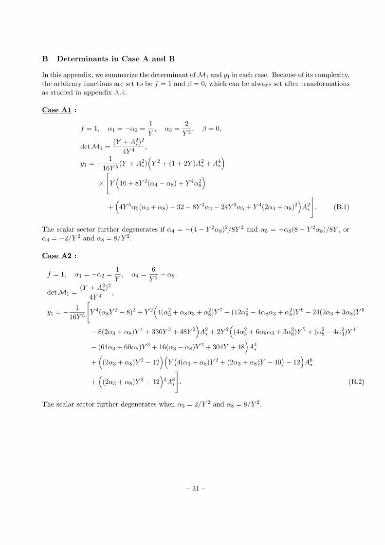
B Determinants in Case A and B

In this appendix, we summarize the determinant ofM1 and y1 in each case. Because of its complexity,the arbitrary functions are set to be f = 1 and β = 0, which can be always set after transformationsas studied in appendix A.4.

Case A1 :

f = 1, α1 = −α2 =1

Y, α3 =

2

Y 2, β = 0,

detM1 =(Y +A2

∗)2

4Y 4,

y1 = − 1

16Y 5(Y +A2

∗)(Y 2 + (1 + 2Y )A2

∗ +A4∗

)×[Y(

16 + 8Y 2(α4 − α8) + Y 4α28

)+(

4Y 5α5(α4 + α8)− 32− 8Y 2α4 − 24Y 3α5 + Y 4(2α4 + α8)2)A2

∗

]. (B.1)

The scalar sector further degenerates if α4 = −(4 − Y 2α8)2/8Y 2 and α5 = −α8(8 − Y 2α8)/8Y , orα4 = −2/Y 2 and α8 = 8/Y 2.

Case A2 :

f = 1, α1 = −α2 =1

Y, α4 =

6

Y 2− α8,

detM1 =(Y +A2

∗)2

4Y 4,

y1 = − 1

16Y 5

[Y 4(α8Y

2 − 8)2 + Y 2(

4(α23 + α8α3 + α2

8)Y 7 + (12α23 − 4α8α3 + α2

8)Y 6 − 24(2α3 + 3α8)Y 5

− 8(2α3 + α8)Y 4 + 336Y 3 + 48Y 2)A2

∗ + 2Y 2(

(4α23 + 6α8α3 + 3α2

8)Y 5 + (α28 − 4α2

3)Y 4

− (64α3 + 60α8)Y 3 + 16(α3 − α8)Y 2 + 304Y + 48)A4

∗

+(

(2α3 + α8)Y 2 − 12)(Y(4(α3 + α8)Y 2 + (2α3 + α8)Y − 40

)− 12

)A6

∗

+(

(2α3 + α8)Y 2 − 12)

2A8∗

]. (B.2)

The scalar sector further degenerates when α3 = 2/Y 2 and α8 = 8/Y 2.

– 31 –

Case A3 :

f = 1, α1 = −α2 = −1

2(α4 + α8)Y,

α3 = −1

4(4α4 + 2α8) +

1

4α8(α4 + α8),

detM1 =

(2α6 + Y (Y α6 − 1)(α4 + α8)

)2(Y +A2

∗)2

16Y 2,

y1 = − 1

128

[2α8(Y 2α8 − 16) +

(3α2

8 (α4 + α8)Y 3 − 64α5 − 8α8 (2α4 + α8)Y)A2

∗

]

×[

4Y +(

8− 4Y (α4 + α8) + Y 2(1 + Y )2(α4 + α8)2)A2

∗ + Y 2(α4 + α8)2A4∗

]. (B.3)

The scalar sector further degenerates when α5 = α8 = 0, α5 = 8(20 + Y 2α4)/Y 3 and α8 = 16/Y 2,or α4 = −α8 = −α5/2Y = −16/Y 2.

Case A4 :As proved in section 3.4.1, the case A4 can be mapped to the GP theory through the transformations(A.1) and (A.2). Therefore, it is not needed to explicitly show the results of the determinant of M1

and y1 here since these properties will not change though transformations as long as a transformationis invertible. The determinant ofM1 and y1 are already shown in section 3.2. If a theory cannot beobtained from an invertible transformation, one needs to directly check the determinant of M1 andy1 in the case A4. As an example, in the case of (3.45),

detM1 =1

16

[2(α6 + α2α6 − α2)Y +

(6 + 4α2 − α7Y − α2α7Y

)A2

∗

]2

,

y1 =1

2(1 + α2)2(6 + β)(3 +A2

∗)A2∗. (B.4)

Case B1 :

f = 1, β = 0, α4 = −2α1

Y, α5 =

(2α1 − Y α3)2

4Y 2(α1 + α2), α8 = 0,

detM1 =(α1 + α6 − Y α1α6)2(Y +A2

∗)2

4Y 2,

y1 =1

2Y 2(α1 + α2)

[4Y 2(α1 + α2)2 + Y

(4α1

(2α2(1 + Y α2) + α1(3 + 2Y α2)

)+ 4Y

(α1Y (α1 + α2)− 2α1 − α2

)α3 + Y 2α2

3

)A2

∗

+(

2Y 2α23 − 8Y α1α3 + α2

1

(8 + Y (1 + Y )(2α2 + Y α3)2

))A4

∗

+ α1(2α2 + Y α3)(

2α1(α2 + Y α2 − 2) + Y (2 + α1 + Y α1)α3

)A6

∗

+ α21(2α2 + Y α3)2A8

∗

]. (B.5)

– 32 –

In this case, y1 is always non-zero for any free functions.

Case B2 :

f = 1, β = 0, α1 =1

Y, α4 = − 2

Y 2, α8 =

8

Y 2,

detM1 =(Y +A2

∗)2

4Y 4,

y1 =1

4Y 5

[8Y (1 + Y α2) +

(4 + 8Y α2 + 4Y 2α3 − Y 4α2

3 + 4Y 3(1 + Y α2)α5

)A2

∗

]×(Y 2(3 + Y ) + 2(Y − 1)Y A2

∗ + (1 + 2Y )A4∗ +A6

∗

). (B.6)

The scalar sector further degenerate when α2 = −1/Y and α3 = 2/Y 2.

Case B3 :

f = 1, β = 0, α1 =1

Y, α4 = − 2

Y 2+ α8 −

Y 2α28

8,

α5 =(2− Y 2α3)2

4Y 3(1 + Y α2)− α8

Y+Y α2

8

8,

detM1 =(Y +A2

∗)2

4Y 4,

y1 =1

128Y 3(α2Y + 1)(A2

∗ + Y )[4Y (α2Y + 1) 2

(α2

8(4Y + 3)Y 3 − 32α8Y2 + 64

)+

(512 + α2

3Y4(α8Y

2 − 8)

2 − 4α3Y2(α8Y

2 − 8) (

20α22α

28Y

6 + 48α2α28Y

5

− 8α8

(16α2

2 + (α2 − 4)α8

)Y 4 − α8 (α2 (64α2 + 319) + 8α8)Y 3

+(256α2

2 − 65α8α2 − 254α8

)Y 2 + (512α2 − α8)Y − 8

))A2

∗

+(

16α2 − α3α8Y3 + 2 (4α3 + α8)Y

)(16 (α2 − 2)− 2α3α8Y

4 + (4α2 − α3)α8Y3

+ 8 (2α3 + α8)Y 2 + 2 (4α3 + α8)Y

)A4

∗

+(16α2 − α3α8Y

3 + 2 (4α3 + α8)Y)

2A6∗

]. (B.7)

In this case, y1 is always non-zero for any free functions.

– 33 –

Case B4 :

f = 1, β = 0, α4 = − 16

Y 2− 2α1

Y, α8 =

16

Y 2,

α5 =

64 + Y

[4α1(8− 7Y α1)− 64(−2 + Y α1)α2 + 4Y (−4 + 3Y α1)α3 + Y 3α2

3

]4Y 4(α1 + α2)

,

detM1 =(α1 + α6 − Y α1α6)2(Y +A2

∗)2

4Y 2,

y1 =1

2(α1 + α2)Y 4

[12 (α1 + α2) 2Y 3(3Y + 4) +

(α2

3Y5 +

(4α2

1(3Y + 2)Y 4

+ 4α1Y4(α2(3Y + 2)− 2

)− 4Y 3 (5α2Y + 4)

)α3

)A2

∗

+

((α2

1Y (Y + 1) + 2)α2

3Y4 −

(8α3

1(Y + 1)Y 4 − 24α1α2(Y + 1)Y 3

+ 4α21Y

3(Y + 1) (5α2Y − 2) + 8Y 2 (3α2Y + 4))α3

+ 4α21(2α1 + 5α2)2Y 4 + 4α1

(4α3

1 + 4(5α2 − 2)α21

+ α2(25α2 − 44)α1 − 60α22

)Y 3 + 4

((2− 44α2)α2

1 − 8α31

+ 20(1− 3α2)α2α1 + 52α22

)Y 2 + 64α2(α1 + 2α2 + 3)Y + 128

)A4

∗

+(

8α2 + α1Y (α3Y − 4α1 − 10α2))(

2(4α2 + α3Y

2 − 8)− 4α2

1Y (Y + 1)

+ α1Y ((Y + 1) (α3Y − 10α2) + 4)

)A6

∗

+

(8α2 + α1Y (α3Y − 4α1 − 10α2)

)2

A8∗

]. (B.8)

In this case, y1 is always non-zero for any free functions.

Case B5 :

f = 1, β = 0, α1 =−8(2α2 + Y α3) + Y (−4− 4Y α2 + Y 2α3)α8

2Y 2α8

α4 =4(1 + Y α2)

Y 2− α3 +

8(2α2 + Y α3)

Y 3α8+ α8 −

Y 2α28

8,

α5 =−2 + Y 2α3

Y 3− 4(2α2 + Y α3)

Y 4α8− α8

Y+Y α2

8

8+

12(2α2 + Y α3)

Y 2(−8 + Y 2α8),

– 34 –

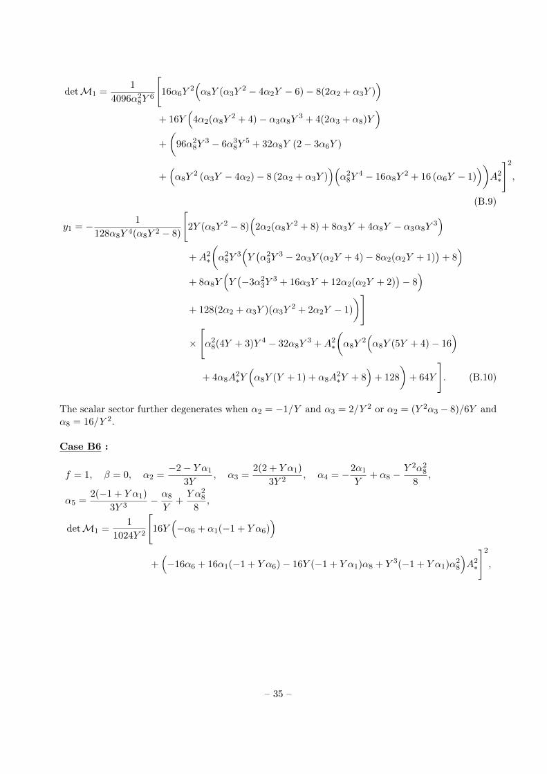
detM1 =1

4096α28Y

6

[16α6Y

2(α8Y (α3Y

2 − 4α2Y − 6)− 8(2α2 + α3Y ))

+ 16Y(

4α2(α8Y2 + 4)− α3α8Y

3 + 4(2α3 + α8)Y)

+

(96α2

8Y3 − 6α3

8Y5 + 32α8Y (2− 3α6Y )

+(α8Y

2 (α3Y − 4α2)− 8 (2α2 + α3Y ))(α2

8Y4 − 16α8Y

2 + 16 (α6Y − 1)))

A2∗

]2

,

(B.9)

y1 = − 1

128α8Y 4(α8Y 2 − 8)

[2Y (α8Y

2 − 8)(

2α2(α8Y2 + 8) + 8α3Y + 4α8Y − α3α8Y

3)

+A2∗

(α2

8Y3(Y(α2

3Y3 − 2α3Y (α2Y + 4)− 8α2(α2Y + 1)

)+ 8)

+ 8α8Y(Y(−3α2

3Y3 + 16α3Y + 12α2(α2Y + 2)

)− 8)

+ 128(2α2 + α3Y )(α3Y2 + 2α2Y − 1)

)]

×[α2

8(4Y + 3)Y 4 − 32α8Y3 +A2

∗

(α8Y

2(α8Y (5Y + 4)− 16

)+ 4α8A

2∗Y(α8Y (Y + 1) + α8A

2∗Y + 8

)+ 128

)+ 64Y

]. (B.10)

The scalar sector further degenerates when α2 = −1/Y and α3 = 2/Y 2 or α2 = (Y 2α3 − 8)/6Y andα8 = 16/Y 2.

Case B6 :

f = 1, β = 0, α2 =−2− Y α1

3Y, α3 =

2(2 + Y α1)

3Y 2, α4 = −2α1

Y+ α8 −

Y 2α28

8,

α5 =2(−1 + Y α1)

3Y 3− α8

Y+Y α2

8

8,

detM1 =1

1024Y 2

[16Y

(−α6 + α1(−1 + Y α6)

)+(−16α6 + 16α1(−1 + Y α6)− 16Y (−1 + Y α1)α8 + Y 3(−1 + Y α1)α2

8

)A2

∗

]2

,

– 35 –

y1 =1

48Y 3(−1 + Y α1)(Y +A2

∗)

×[

64Y − 32Y 3α8 + Y 4(3 + 4Y )α28 +A2

∗

(128 + Y 2α8(−16 + Y (4 + 5Y )α8)

+ 4Y α8A2∗(8 + Y (1 + Y )α8 + Y α8A

2∗))]. (B.11)

The scalar sector further degenerates when α1 = 1/Y .

C Case C : General theories with f = 0

In this appendix, we investigate a remaining subclass of degenerate theories where the Einstein-Hilbert term is absent, i.e., f = 0. In this case, the first condition D0(Y ) = 0 is automaticallysatisfied since Q vanishes with f = fY = 0, as can be seen in (3.4). Then, we have

0 =1

16α1Y

(2α1 + Y (α4 + α8)− β

)×[

4α1 (α1 + 4α2) + 4(

3α2α4 + α1 (α3 + α4))Y +

(4 (α1 + 3α2)α5 − 3α2

3

)Y 2

]. (C.1)

Thus, we have four branches here.

α1 = 0 or α4 =β − 2α1 − Y α8

Yor

α4 =3Y 2α2

3 − 4α1(α1 + 4α2)− 4Y α1α3

4Y (α1 + 3α2)− Y α5 or α1 = −3α2. (C.2)

Here, we assumed α1 + 3α2 6= 0 in the third branch. In the first branch, we automatically haveD1(Y ) = 0, thereforeCase C1 :

f = α1 = 0.

(C.3)

Note that the case C1 corresponds to the ”class IIIc” in [19]. In this case, the other determinantsare all zero, detM1 = detM2 = 0. The second branch in (C.1) provide us the following condition,

0 = D1(Y ) = − 1

16α1Y (α1 + 3α2) (α8Y − 2β) 2. (C.4)

The first solution corresponds to the case C1, then we have two solutions,Case C2 :

f = 0, α1 = −3α2, α4 =6α2 − Y α8 + β

Y, (C.5)

Case C3 :

f = 0, α4 = −2α1 + β

Y, α8 =

2β

Y. (C.6)

– 36 –

Note that this case includes the special case of the beyond GP theory with f = 0 when α1 = −α2,α3 = −α4, and β = 0. The third branch in (C.1) gives

0 = D1(Y ) =1

16α1Y

[−4α1 (α1 + 2α2)β + 4α1α3βY −

(3α2

3β + (α1 + 3α2)(α28 − 4α5β)

)Y 2

].(C.7)

Then, solving for α5, we haveCase C4 :

f = 0, α4 = −2α1

Y− Y α2

8

4β, α5 =

4α1(α1 + 2α2)− 4Y α1α3 + 3Y 2α23

4Y 2(α1 + 3α2)+α2

8

4β. (C.8)

where α1 + 3α2 6= 0 is assumed since the case α1 + 3α2 = 0 is studied in the case C2. Note that thiscase includes the beyond GP theory with f = 0 and β 6= 0 when α1 = −α2, α3 = −α4, and α8 = 0.We have an additional solution in the third branch, which is β = 0. In this case, D1(Y ) is given by

0 = D1(Y ) = − 1

16Y 3α1(α1 + 3α2)α2

8. (C.9)

The first solution corresponds to the case C1. Since α1 + 3α2 6= 0 in this branch, we only have onesolution,Case C5 :

f = 0, α4 =3Y 2α2

3 − 4α1(α1 + 4α2)− 4Y α1α3

4Y (α1 + 3α2)− Y α5, β = α8 = 0. (C.10)

The last branch in (C.1) gives

0 = − 9

16Y α2(2α2 + Y α3)2

(6α2 − Y (α4 + α8) + β

). (C.11)

Then, the first solution α2 = 0 immediately leads to α1 = 0, which is included in the case C1. Thesecond solution givesCase C6 :

f = 0, α1 =3Y α3

2, α2 = −Y α3

2. (C.12)

The last solution is exactly the same one as obtained in the case C2.

References

[1] S. Perlmutter et al., Measurements of Ω and Λ from 42 High-Redshift Supernovae, Astrophys. J 517(1999) 565–586, [astro-ph/9812133], [doi:10.1086/307221].

[2] A. G. Riess et al., Observational Evidence from Supernovae for an Accelerating Universe and aCosmological Constant, Astron. J 116 (1998) 1009–1038, [astro-ph/9805201], [doi:10.1086/300499].

[3] T. Clifton, P. G. Ferreira, A. Padilla, and C. Skordis, Modified gravity and cosmology, Phys. Rept. 513(2012) 1–189, [arXiv:1106.2476], [doi:10.1016/j.physrep.2012.01.001].

[4] S. Tsujikawa, Modified Gravity Models of Dark Energy, Lect.Notes Phys. 800 (2010) 99–145,[arXiv:1101.0191].

– 37 –

[5] A. Nicolis, R. Rattazzi, and E. Trincherini, Galileon as a local modification of gravity, Phys. Rev. D 79(2009) 064036, [arXiv:0811.2197], [doi:10.1103/PhysRevD.79.064036].

[6] A. Nicolis and R. Rattazzi, Classical and Quantum Consistency of the DGP Model, JHEP 6 (2004) 059,[hep-th/0404159], [doi:10.1088/1126-6708/2004/06/059].

[7] M. A. Luty, M. Porrati, and R. Rattazzi, Strong interactions and stability in the DGP model, JHEP 9(2003) 029, [hep-th/0303116], [doi:10.1088/1126-6708/2003/09/029].

[8] G. Dvali, G. Gabadadze, and M. Porrati, 4D gravity on a brane in 5D Minkowski space, Physics LettersB 485 (2000) 208–214, [hep-th/0005016], [doi:10.1016/S0370-2693(00)00669-9].

[9] C. de Rham and G. Gabadadze, Generalization of the Fierz-Pauli action, Phys. Rev. D 82 (2010)044020, [arXiv:1007.0443], [doi:10.1103/PhysRevD.82.044020].

[10] C. de Rham, G. Gabadadze, and A. J. Tolley, Resummation of Massive Gravity, Phys. Rev. Lett. 106(2011) 231101, [arXiv:1011.1232], [doi:10.1103/PhysRevLett.106.231101].

[11] C. Deffayet, G. Esposito-Farese, and A. Vikman, Covariant Galileon, Phys. Rev. D 79 (2009), no. 8084003, [arXiv:0901.1314], [doi:10.1103/PhysRevD.79.084003].

[12] G. W. Horndeski, Second-order scalar-tensor field equations in a four-dimensional space, Int. J. Theor.Phys. 10 (1974) 363, [doi:10.1007/BF01807638].

[13] C. Deffayet, X. Gao, D. A. Steer, and G. Zahariade, From k-essence to generalized Galileons, Phys.Rev. D 84 (2011) 064039, [arXiv:1103.3260], [doi:10.1103/PhysRevD.84.064039].

[14] T. Kobayashi, M. Yamaguchi, and J. Yokoyama, Generalized G-Inflation — Inflation with the MostGeneral Second-Order Field Equations —, Progress of Theoretical Physics 126 (2011) 511–529,[arXiv:1105.5723].

[15] J. Gleyzes, D. Langlois, F. Piazza, and F. Vernizzi, New Class of Consistent Scalar-Tensor Theories,Physical Review Letters 114 (2015), no. 21 211101, [arXiv:1404.6495],[doi:10.1103/PhysRevLett.114.211101].

[16] D. Langlois and K. Noui, Degenerate higher derivative theories beyond Horndeski: evading theOstrogradski instability, JCAP 2 (2016) 034, [arXiv:1510.06930], [doi:10.1088/1475-7516/2016/02/034].

[17] D. Langlois and K. Noui, Hamiltonian analysis of higher derivative scalar-tensor theories, JCAP 07(2016) 016, [arXiv:1512.06820].

[18] M. Crisostomi, K. Koyama, and G. Tasinato, Extended scalar-tensor theories of gravity, JCAP 4 (2016)044, [arXiv:1602.03119], [doi:10.1088/1475-7516/2016/04/044].

[19] J. Ben Achour, D. Langlois, and K. Noui, Degenerate higher order scalar-tensor theories beyondHorndeski and disformal transformations, Phys. Rev. D 93 (2016) 124005, [arXiv:1602.08398].

[20] C. de Rham and A. Matas, Ostrogradsky in Theories with Multiple Fields, JCAP 06 (2016) 041,[arXiv:1604.08638].

[21] G. Gabadadze, K. Hinterbichler, D. Pirtskhalava, and Y. Shang, Potential for general relativity and itsgeometry, Phys. Rev. D 88 (2013), no. 8 084003, [arXiv:1307.2245], [doi:10.1103/PhysRevD.88.084003].

[22] N. A. Ondo and A. J. Tolley, Complete decoupling limit of ghost-free massive gravity, JHEP 11 (2013)59, [arXiv:1307.4769], [doi:10.1007/JHEP11(2013)059].

[23] C. Deffayet, A. E. Gumrukcuoglu, S. Mukohyama, and Y. Wang, A no-go theorem for generalized vectorGalileons on flat spacetime, JHEP 4 (2014) 82, [arXiv:1312.6690], [doi:10.1007/JHEP04(2014)082].

[24] G. W. Horndeski, Conservation of charge and the Einstein-Maxwell field equations, Journal ofMathematical Physics 17 (1976) 1980–1987, [doi:10.1063/1.522837].

[25] L. Heisenberg, Generalization of the Proca Action, JCAP 5 (2014) 015, [arXiv:1402.7026],

– 38 –

[doi:10.1088/1475-7516/2014/05/015].

[26] E. Allys, P. Peter, and Y. Rodrıguez, Generalized Proca action for an Abelian vector field, JCAP 2(2016) 004, [arXiv:1511.03101], [doi:10.1088/1475-7516/2016/02/004].

[27] J. Beltran Jimenez and L. Heisenberg, Derivative self-interactions for a massive vector field, PhysicsLetters B 757 (2016) 405–411, [arXiv:1602.03410], [doi:10.1016/j.physletb.2016.04.017].

[28] L. Heisenberg, R. Kase, and S. Tsujikawa, Beyond generalized Proca theories, Phys.Lett. B 760 (2016)617–626, [arXiv:1605.05565].

[29] A. De Felice, L. Heisenberg, R. Kase, S. Mukohyama, S. Tsujikawa, and Y.-l. Zhang, Effectivegravitational couplings for cosmological perturbations in generalized Proca theories, Phys. Rev. D 94(2016) 044024, [arXiv:1605.05066].

[30] A. De Felice, L. Heisenberg, R. Kase, S. Mukohyama, S. Tsujikawa, and Y.-l. Zhang, Cosmology ingeneralized Proca theories, JCAP 06 (2016) 048, [arXiv:1603.05806],[doi:10.1088/1475-7516/2016/06/048].

[31] L. Heisenberg, R. Kase, and S. Tsujikawa, Anisotropic cosmological solutions in massive vector theories,arXiv:1607.03175.

[32] M. Hull, K. Koyama, and G. Tasinato, A Higgs Mechanism for Vector Galileons, JHEP 03 (2015) 154,[arXiv:1408.6871].

[33] M. Hull, K. Koyama, and G. Tasinato, Covariantized vector Galileons, Phys. Rev. D 93 (2016) 064012,[arXiv:1510.07029], [doi:10.1103/PhysRevD.93.064012].

[34] J. Chagoya, G. Niz, and G. Tasinato, Black holes and Abelian symmetry breaking, Classical andQuantum Gravity 33 (2016) 175007, [arXiv:1602.08697], [doi:10.1088/0264-9381/33/17/175007].

[35] P. Fleury, J. P. Beltran Almeida, C. Pitrou, and J.-P. Uzan, On the stability and causality ofscalar-vector theories, JCAP 1411 (2014), no. 11 043, [arXiv:1406.6254],[doi:10.1088/1475-7516/2014/11/043].

[36] E. Allys, J. P. Beltran Almeida, P. Peter, and Y. Rodriguez, On the 4D generalized Proca action for anAbelian vector field, arXiv:1605.08355.

[37] T. Chiba, T. Okabe, and M. Yamaguchi, Kinetically driven quintessence, Phys. Rev. D 62 (2000)023511, [astro-ph/9912463], [doi:10.1103/PhysRevD.62.023511].

[38] C. Armendariz-Picon, V. Mukhanov, and P. J. Steinhardt, Dynamical Solution to the Problem of aSmall Cosmological Constant and Late-Time Cosmic Acceleration, Physical Review Letters 85 (2000)4438–4441, [astro-ph/0004134], [doi:10.1103/PhysRevLett.85.4438].

[39] H. Motohashi, K. Noui, T. Suyama, M. Yamaguchi, and D. Langlois, Healthy degenerate theories withhigher derivatives, JCAP 7 (2016) 033.

[40] A. H. Chamseddine and V. Mukhanov, Mimetic Dark Matter, JHEP 11 (2013) 135, [arXiv:1308.5410],[doi:10.1007/JHEP11(2013)135].

[41] N. Deruelle and J. Rua, Disformal Transformations, Veiled General Relativity and Mimetic Gravity,JCAP 1409 (2014) 002, [arXiv:1407.0825], [doi:10.1088/1475-7516/2014/09/002].

[42] G. Domenech, S. Mukohyama, R. Namba, A. Naruko, R. Saitou, and Y. Watanabe,Derivative-dependent metric transformation and physical degrees of freedom, Phys. Rev. D 92 (2015),no. 8 084027, [arXiv:1507.05390], [doi:10.1103/PhysRevD.92.084027].

– 39 –