Extending the Use and Prediction Precision of Subnational

Public Opinion Estimation*

Lucas Leemann† Fabio Wasserfallen‡

September 2014

Abstract

The comparative study of subnational units is on the rise. To estimate public opinion

on the subnational level, multilevel regression and poststratification (MRP) has become

the standard method. Unfortunately, MRP comes with stringent data requirements, as it

requires data for the joint distribution. As a consequence, scholars cannot apply MRP in

countries without a census, and when census data is available, the modeling is restricted to

a few variables. This article introduces multilevel regression with marginal poststratifica-

tion (MRmP), which relies on marginal distributions only. The relaxed data requirement

increases the prediction precision of the method and extends the use of MRP to coun-

tries without census data. Monte Carlo analyses as well as U.S. and Swiss applications

show that, using the same predictors, MRmP performs as well as the current standard

approach, and it is superior when additional predictors are modeled. These improvements

promise that MRmP will further stimulate subnational research.

∗Many thanks to Noah Buckley, Andrew Gelman, Andy Guess, Jonathan Kastellec, Romain Lachat, JeffLax, Tiffany Washburn, and Piero Stanig for helpful comments. We also thank Christopher Warshaw andJonathan Rodden for sharing their data with us and Werner Seitz and his team at the Swiss Federal StatisticsOffice for the ongoing supply of various data sets. Patrice Siegrist provided excellent research assistance. Thefinancial support from the Swiss National Science Foundation is gratefully acknowledged (grants #: 100017-1377651 and P1SKP1-148357).

†Department of Political Science, University College London, UK. Email: l.leemann@ucl.ac.uk URL: http://www.ucl.ac.uk/~uctqltl.

‡Assistant Professor, University of Salzburg, Austria; Associate Research Scholar, Princeton University,U.S.A. Email: fabio.wasserfallen@sbg.ac.at URL: www.fabiowasserfallen.ch.

1 Introduction

The comparative study of subnational units attracts growing interest in the literature. There

are a number of reasons for this: subnational units are potentially better suited for comparative

analysis than countries because they are less heterogeneous, more accurate data is available,

country-specific factors are constant, and controlled comparisons allow to develop interesting

identification strategies for causal inference (e.g., Snyder, 2001; Ziblatt, 2008; Tausanovitch

and Warshaw, 2014). A critical but challenging element of subnational comparative research

is the estimation of public opinion. The recent introduction of hierarchical modeling and

poststratification, so-called MRP, generates reliable public opinion estimates for subnational

units. Unfortunately, the use of MRP, as currently applied in the literature, comes with

stringent data requirements. We build on the recent methodological advances and develop a

new approach that extends the use of MRP beyond a few (post-)industrialized countries and

that increases the prediction precision of the method substantially.

Early attempts in the estimation of public opinion disaggregated national surveys into

subnational subsamples (Miller and Stokes, 1963). One solution for overcoming the small-

n problem of the disaggregation approach was to combine multiple surveys with the same

questions into one mega-poll (Erikson et al., 1993). Gelman and Little (1997), then, laid the

methodological ground work for MRP, which replaced the older methods and can be applied

by using standard national survey data (Lax and Phillips, 2009b; Warshaw and Rodden, 2012).

The quick spread of MRP is quite remarkable—not least when we consider that the method

has, to the best of our knowledge, only been applied in the U.S., U.K., and Switzerland so

far.

The narrow spatial scope is mainly because of the stringent data requirement of the current

standard application of the method. The precondition for using MRP is that detailed census

data in the form of joint distributions is available for poststratification. Researchers need

to know, for example, how many 18–35-year-old women with a university degree live in each

subnational unit. This data requirement makes it impossible to apply MRP in countries where

2

such data is not available—whether this is because of data protection laws (e.g., in India) or

because the data is not gathered by a single agency (e.g., in Afghanistan). Furthermore, if

census data is available, researchers can only use three or four demographic variables that

are provided in the restrictive format of joint distributions as individual-level predictors of

political preferences. Strong predictors such as party identification and income cannot be

modeled.

We develop an alternative application of MRP, which we call multilevel regression with

marginal poststratification (MRmP). MRmP relies on marginal distributions. For applying

MRmP, researchers only need to know, for example, the shares (marginals) of women, of uni-

versity graduates, and of 18–35-year-old citizens in each subnational unit. Due to this relaxed

data requirement, MRmP can be applied in countries where it has not been possible (e.g.,

in India and Afghanistan). A further important advantage of MRmP is that it increases the

prediction precision of subnational public opinion estimation for countries with a census (e.g.,

the U.S. and Switzerland). The findings of U.S. and Swiss data analyses show that the use

of additional strong predictors such as income and party identification beyond the standard

demographic variables improves the prediction precision of MRP substantially. Finally, we

provide pre-modeling guidance to help researchers specify models that derive precise subna-

tional public opinion estimates with MRP. In short, MRmP, the approach developed in this

article, goes beyond the data limitations of the current standard application, extends the use

of MRP, and substantially improves the prediction precision of the still young method. We

thus believe that MRmP will further stimulate comparative research using public opinion

estimates for empirical analysis.

This article first summarizes the standard application of MRP in the literature, which we

call “classic MRP”, before introducing MRmP. The theoretical part then shows that potential

deviations in predictions between MRmP and classic MRP are solely due to the non-constant

marginal effects in the response model. We derive the conditions under which this can make

a difference and further investigate MRmP with Monte Carlo and real-world data analyses.

3

The findings document that MRmP substantially improves upon classic MRP. Finally, we

provide MRP pre-modeling guidance and conclude.

2 “Classic MRP” and Its Limits

The application of MRP has its origins in the Gelman and Little (1997) study, which combined

hierarchical modeling and poststratification. Park et al. (2004) subsequently introduced the

method to political science with a remarkable impact on the discipline, as the substantial

number of recent studies using the approach documents (Lax and Phillips, 2009a,b, 2012;

Kastellec, Lax and Phillips, 2010; Warshaw and Rodden, 2012; Pacheco, 2012; Tausanovitch

and Warshaw, 2014). In the last years, MRP has been established as the state-of-the-art

method for comparative subnational research studying public opinion. Accordingly, Selb

and Munzert (2011, 456) conclude that MRP is the “gold standard” in estimating political

preferences on the subnational level.

MRP estimates public opinion on the subnational level in four steps. The first is to conduct

a survey that identifies personal characteristics and asks a number of political preference

questions; second, a hierarchical model is fitted to the data to make predictions for specific

voter types; in the third step, predictions for all predefined voter types are calculated using the

estimates of the hierarchical model; and, finally, researchers calculate, based on fine-grained

census data, public opinion estimates in the subnational units by weighting the predictions

of each voter type according to the number of voters living in the subnational units with the

same characteristics.

Let us further illustrate the data requirements and the method. Researchers start with the

collection of national survey data of usually somewhere between 500 and 1,500 respondents

and model the responses on the support for a specific policy. For illustrative purposes, we

explore an MRP response model with two individual-level variables – gender (men/women)

and education (no high school, high school, college, post-graduate) – and with random effects

for the subnational unit (αc) and the region (αr). In addition, we include a number of

4

contextual factors explaining variation between the subnational units (Xc). Accordingly, we

write the following hierarchical probit, as a standard response model, to estimate the support

for a specific policy:

Pr(yi = 1) = Φ(β0 + αgender

j[i] + αeducationm[i] + αsubnational unit

c

)αgenderj ∼ N(0, σ2

gender), for j = 1, ..., J

αeducationm ∼ N(0, σ2

education), for m = 1, ...,M

αsubnational unitc ∼ N(αregion

r[c] + βXc, σ2subnational unit), for c = 1, ..., C

αregionr ∼ N(0, σ2

region), for r = 1, ..., R

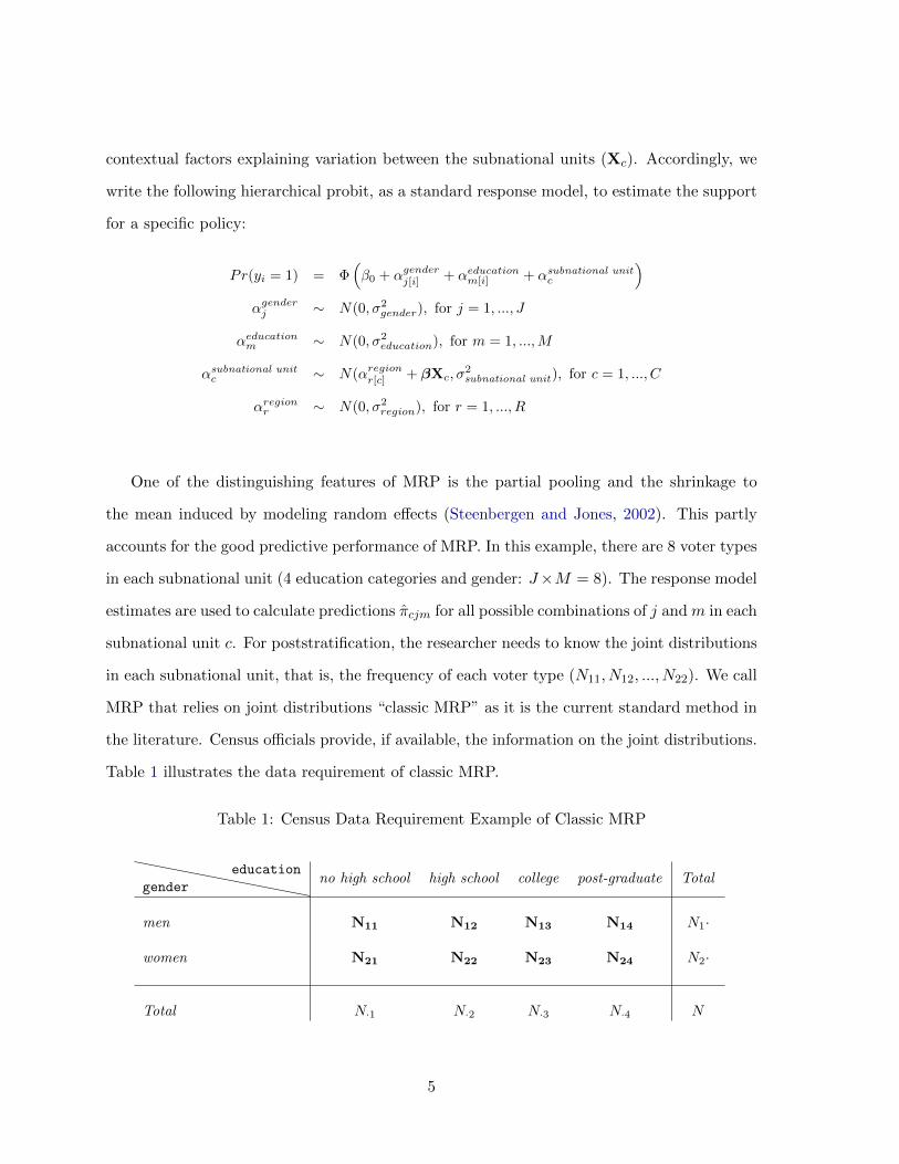
One of the distinguishing features of MRP is the partial pooling and the shrinkage to

the mean induced by modeling random effects (Steenbergen and Jones, 2002). This partly

accounts for the good predictive performance of MRP. In this example, there are 8 voter types

in each subnational unit (4 education categories and gender: J×M = 8). The response model

estimates are used to calculate predictions πcjm for all possible combinations of j and m in each

subnational unit c. For poststratification, the researcher needs to know the joint distributions

in each subnational unit, that is, the frequency of each voter type (N11, N12, ..., N22). We call

MRP that relies on joint distributions “classic MRP” as it is the current standard method in

the literature. Census officials provide, if available, the information on the joint distributions.

Table 1 illustrates the data requirement of classic MRP.

Table 1: Census Data Requirement Example of Classic MRP

gender

educationno high school high school college post-graduate Total

men N11 N12 N13 N14 N1·

women N21 N22 N23 N24 N2·

Total N·1 N·2 N·3 N·4 N

5

Finally, each prediction is weighted by the joint distribution data and the total sum divided

by the number of all residents:

πc =

∑j

∑m πjm∈cNjm∈c

Nn∈c=

∑j

∑m Φ

(β0 + αm + αj + αc

)Njm∈c

Nn∈c

In this example, we rely on eight voter types. Real-world applications include more

individual-level random effects. Lax and Phillips (2009b), for example, work with gender,

three races, and four education and age categories (96 types) and thus need, among others,

data on the exact number of 18–29-year-old black women with a high school degree in each

state. Such fine-grained information is only available if a detailed census has been carried out.

If joint distribution data is available, the specification of the response model is pre-determined

by the data of the census bureau (not the modeling decisions of researchers) and usually re-

stricted to standard demographic variables. The demanding data requirements of classic MRP

are problematic for the following reasons:

• In developing countries, fine-grained census data is not available. In Afghanistan, for

example, no census is carried out, while in the more developed India, census data on

the village level is not available as a joint distribution.

• The joint distributions of the census in (post-)industrialized countries do not include

variables that are potentially important predictors of political preferences. Party iden-

tification, for example, is neither available in the Swiss nor in the U.S. census as joint

distributions.

Before political scientists started working with MRP, the standard method for deriving

preference measures on the subnational level was the disaggregation of national surveys into

subnational samples. While this method is free from data availability restrictions, the esti-

mates for small constituencies are unreliable, as they stem from very few observations (Lev-

endusky et al., 2008). Several studies have shown that MRP estimates are more precise than

6

disaggregation estimates (e.g., Lax and Phillips, 2009b). Following the MRP literature, we use

disaggregation estimates as a baseline measure to gauge the extent to which MRP improves

predictive precision. Our main goal in this analysis is to build on the strength of MRP by

relaxing the strict data requirements of the current standard application in the literature.

3 MRP with Synthetic Joint Distributions (MRmP)

Even some of the most sophisticated MRP contributions are constrained by the data require-

ments discussed above. Warshaw and Rodden (2012, 208), for example, study district-level

public opinion in the U.S. without using age as a predictor in their response model because

the “census factfinder does not include age breakdowns for each race/gender/education sub-

group.” This example highlights the data availability problem of classic MRP: while U.S.

district data on the age structure is available as a marginal distribution, data on the exact

number of elderly people with a given gender, age, and education is not. More generally,

marginal distributions are available for many interesting variables in most countries. In the

Afghan case, for example, the Asia Foundation collects data on the ethnic and linguistic

structures of subnational populations.

The key deviation of MRmP, the approach developed in this article, is that it relies on

synthetic joint distributions that are created with data on the marginal distributions (while

classic MRP relies on the “true” joint distributions). Our point of departure is that researchers

can collect data on the population structures of subnational units as marginal distributions

for various variables that are potentially important predictors of political preferences. Instead

of relying exclusively on the demographic variables of the census, MRmP allows the modeling

of any political, social, economic, or demographic variable asked in the survey. Researchers

only need the marginal distributions of these variables in the subnational units, which are

more widely available.

7

MRmP calculates the synthetic joint distributions for the poststratification step with data

on the marginal distributions. The synthetic joints can be computed in two different ways:

either by extracting the data from multiple surveys (Kastellec et al., 2014), or, as we propose,

by estimating the product of the marginal distributions as a rough approximation of the true

joint distribution. The estimated synthetic joint will be correct, when the used variables are

independent of one another. If they are not—which is in all likelihood the case—the synthetic

joint will deviate from the true joint distributions. However, as we will show, the deviation

only affects the MRP predictions through the non-constant marginal effects of the probit link

function in the response model. In terms of prediction precision, the differences are essentially

irrelevant, as the findings of the Monte Carlo simulations and the real-world data applications

show. We will come back to this shortly.

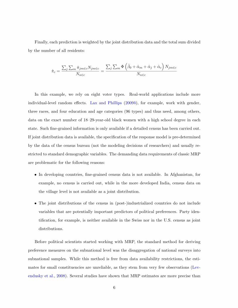
The following theoretical discussion illustrates the difference between classic MRP and

MRmP by emphasizing the scenario under which the two estimation procedures are most

distinct. Table 2 shows an example of two binary individual-level variables, v1 and v2, that are

completely separated and thus totally dependent. The synthetic joint distribution, estimated

as the product of the marginal distributions (60% and 40%), deviates quite strongly from the

true joint distribution in this most extreme case (compare Table 2.1 and 2.2).

Table 2: True and Synthetic Joint Distributions for the Most Extreme Case

v1

v2i=1 i=2

j=1 60% 0% 60%

j=2 0% 40% 40%

60% 40% 100%

2.1: True Joint Distribution

papa

v1

v2i=1 i=2

j=1 36% 24% 60%

j=2 24% 16% 40%

60% 40% 100%

2.2: Synthetic Joint Distribution

papa

v1

v2i=1 i=2

j=1 7% 50%

j=2 69% 98%

2.3: Predicted Support

Notes: Example of a synthetic joint distribution for the most extreme case where the two individual-levelvariables are fully dependent. The predicted support in Table 2.3 is based on a model that includes tworandom effects (αv1 and αv2) with the following estimates: αv1

1 = −1, αv12 = +1, αv2

1 = −0.5, and αv22 = +1.

8

What matters for applied scholars is how much the predictions differ with the use of the

synthetic joint distribution (MRmP) compared to the true joint distribution (classic MRP).

To estimate the difference in predictions, we assume a response model, which is identical in

both procedures, with two random effects on the individual level (age and education) and

an estimated constant with the value 0. As estimates for the random effects, we pick fairly

large numbers (from −1 to +1) to magnify the difference between classic MRP and MRmP. In

applied work, random effects are clearly smaller (see Appendix A.3). The predicted probability

for an individual of a specific cell is estimated using the random effects (e.g., for an individual

from the upper left cell: p11 = Φ(αv11 + αv2

1 )). Table 2.3 reports the predicted support for each

cell based on the response model estimates. The support in the subnational unit is estimated

by weighting the predictions for each type by its frequency in the population. With the true

joint distribution (classic MRP, see Table 2.1), the support in the subnational unit, ptrue, is

estimated as follows:

ptrue = 0.6 · Φ(αv11 + αv2

1 ) + 0.4 · Φ(αv12 + αv2

2 )

= 0.6 · Φ(−1.5)︸ ︷︷ ︸0.07

+ 0.4 · Φ(+2)︸ ︷︷ ︸0.98

= 0.431

Using the synthetic joint distribution (MRmP, see Table 2.2), the support in the subna-

tional unit, psyn, is estimated as follows:

psyn = 0.24 · Φ(αv11 + αv2

2 )︸ ︷︷ ︸should be 0% of pop

+ 0.36 · Φ(αv11 + αv2

1 )︸ ︷︷ ︸should be 60% of pop

+ 0.24 · Φ(αv12 + αv2

1 )︸ ︷︷ ︸should be 0% of pop

+ 0.16 · Φ(αv12 + αv1

2 )︸ ︷︷ ︸should be 40% of pop

= 0.24 · Φ(0)︸︷︷︸0.5

+ 0.36 · Φ(−1.5)︸ ︷︷ ︸0.07

+ 0.24 · Φ(+0.5)︸ ︷︷ ︸0.69

+ 0.16 · Φ(+2)︸ ︷︷ ︸0.98

= 0.466

9

In this most extreme example, the deviation in predicted support is only 3.5%. The pre-

diction deviation is surprisingly small, considering that we choose variables that are perfectly

correlated and high values for the estimated random effects. To understand the source of the

deviation, it is important to recall that the synthetic joint distribution is computed using the

correct marginal distributions: it accounts for 60% of the population with the characteristic

v1 = 1, for 60% with v2 = 1, for 40% with v1 = 2, and for 40% with v2 = 2; wrong are only

the joint distribution values. However, the prediction deviation of 3.5% is not so much a prod-

uct of the wrong synthetic joint distribution values but rather because of the non-constant

marginal effects of the probit link function in the response model. In a probit model, adding

αv11 to a hypothetical person with v2 = 0 has a different marginal effect than it has on a

person with v2 = 1.

Let us illustrate that point by looking at how the support in the subnational unit is

estimated in both procedures. In this illustrative case, all individuals of the first row of the

matrix (v1 = 1) also have the characteristic v2 = 1 (see Table 2.1). For example, all women

are also university graduates (and no man has a university degree). Accordingly, women’s

predicted support of 7% for the policy is weighted by 0.6 (see the first part of the equation

using the true joint distribution). In the estimation with the synthetic joint distribution,

women’s predicted support is overestimated, as the 7% support is only weighted by 0.36 (see

the second part of the equation using the synthetic joint distribution), while the additional

0.24 of women (with the characteristic v1 = 1, i.e., no university degree) is multiplied with a

higher predicted probability of 50% (see the first part of the equation using the synthetic joint

distribution). As there are no women with no university degree in that illustrative example,

women’s predicted support for the policy is overestimated.

For men (v1 = 2), the equation using the true joint distribution weights the very high

98% probability of men’s support for the policy by 0.40. The prediction using the synthetic

joint distribution, however, underestimates men’s support for the policy, as it weighs the 98%

support only for 0.16 and adds 0.24 with 69% support. Overall, MRmP overestimates women’s

10

and underestimates men’s support for the policy in this example. In a linear model, this over-

and underestimation of predicted support between men and women would cancel each other

out—but not in a probit model: the non-constant marginal effects in a probit model explain the

small prediction deviation between classic MRP and MRmP of 3.5%.1 Based on this analysis,

we derive two important implications. First, the deviation in predictions between classic MRP

and MRmP is only because of the non-linear link function of the probit model. Second, the

non-constant marginal effects of the probit model only cause deviations in predictions to the

extent to which the individual-level variables are correlated.

MRmP is related to raking, a procedure in survey methodology, which is an alternative

to poststratification when only marginal distributions are available. Raking works as follows:

weights are assigned based on one of the marginal distributions and then, conditional on the

derived weights, new weights are calculated based on the marginal distribution of the second

variable, and so on. This estimation process, known as iterative proportional fitting, is re-

peated until the marginals of the weighted sample converge to the marginals of the population

and is applied when the sample is not representative (Deming and Stephan, 1940; Fienberg,

1970). Unlike raking, MRmP does not create weights for every single observation, but rather

a weight for each ideal type as specified in the response model. What is similar, however, is

that both methods rely on marginal distributions instead of joint distributions.

Table 3 summarizes the distinction between classic MRP and MRmP. The most important

advantage of MRmP is that it allows the modeling of individual-level variables, of which only

the marginal distributions are available, while having data on the true joint distribution is

a conditio sine qua non for classic MRP. MRmP thus extends the use of MRP to countries

without a census and makes the application of MRP more flexible for countries where census

data is available.

1Note that in the linear case, the two equations predicting public opinion are identical. We have exploredMRP with a linear model, as there is something like a folk theorem (at least among economists) that a linearmodel performs as well as a probit model for binary outcomes (Angrist and Pischke, 2008; Beck, 2011). However,MRP with a linear model does not perform optimally. The main problem is that it tends to produce estimatesthat are less than 0 or greater than 1. This is one of the criticisms of using linear models for binary outcomevariables (Maddala, 1983, 16).

11

Table 3: Date Requirement and Model Flexibility of Classic MRP and MRmP

MRmP Classic MRP

True joint distribution needed " X

Marginal distributions are sufficient X "

Flexible modeling of response model X "

The potential downside of MRmP is that the correlation between individual-level variables

induces a small deviation in prediction because of the non-constant marginal effects of the

probit model.2 The discussed illustrative example explored the most extreme (and unrealistic)

case with a perfect correlation between the two variables. If they were totally independent—

which is also unrealistic—classic MRP and MRmP would provide the same results. In general,

the deviation between the predictions becomes larger as the correlation increases.3 The de-

viation in prediction between the two MRP approaches also increases with higher variances

of the random effects. The next sections analyze whether MRmP performs as well as MRP

in applied settings, and whether MRmP outperforms classic MRP when additional, powerful,

individual-level predictors are modeled.

2A second limitation is that deep interactions can only be modeled if the two constituting variables areavailable in the census data (Ghitza and Gelman, 2013).

3See Appendix A.1 for correlations in Swiss and U.S. data.

12

4 MRmP and Classic MRP with the Same Data

Should we expect that predictions differ between MRP and MRmP in applied work? To

answer that question, we execute Monte Carlo analyses with two manipulated parameters:

first, we change the sample sizes from a small sample of 500 respondents to a medium sample

of 1,000 respondents and a large sample of 2,000 respondents. Second, we use four different

correlations (ρ) among the individual-level variables (0, 0.2, 0.4, and 0.6). In the case of no

correlation, MRmP and classic MRP are equivalent (with perfect independence, the product of

the marginals equals the true joint distribution). Correlations of 0.2 and partly also of 0.4 are

realistic for standard demographic values, while 0.6 is exceptionally high (see Appendix A.1).

As discussed in the previous section, the prediction deviation between the two procedures

should increase as the correlation becomes larger.

The data-generating-process (DGP) assumes three variables on the individual level and

a variable on the subnational level. We analyze 25 subnational units; 10 of them are large

(each covering 7% of the total population) and 15 are small (each covering 3% of the total

population). The following equations describe the DGP:

y∗i = β0 + γ1[i] + γ2[i] + γ3[i] + αsubnational unitc + εic

Pr(yi = 1) = Φ(y∗i ), εic ∼ N(0, 4)

γ1i ∼ N(0, 1) & γ2i ∼ N(0, 1) & γ3i ∼ N(0, 1)

αsubnational unitc ∼ N(Xc, 4), for c = 1, ..., 25

The individual-level variables (γ1, γ2, γ3) are based on draws from a multivariate normal

distribution and transformed to discrete variables with four categories each:

γki =

1 if γki < −1,

2 if − 1 < γki < 0,

3 if 0 < γki < 1,

4 if γki > 1

and Var(γ) =

1 ρ ρ

ρ 1 ρ

ρ ρ 1

for k =1, 2, 3.

13

The selected random effects (γki) are quite large in size as they are based on the following

normal distributions (γk ∼ N(0, 1), ∀ k). In real-world examples, the random effects are

smaller (the conservative setup of the analysis tends to overestimate the prediction deviation

between classic MRP and MRmP).4 The subnational level variable, Xc, is evenly spread

between −2 and +2. For the Monte Carlo analyses, we create a “true” population of one

million citizens, draw for every simulation a new sample, and estimate disaggregation, classic

MRP, and MRmP predictions.

Figure 1 shows the prediction precision for 12 different Monte Carlo analyses (with three

different sample sizes and four different correlations) for disaggregation, classic MRP, and

MRmP. Each of the three plots reports the simulation results for the four different correla-

tions (0, 0.2, 0.4, 0.6) of the individual-level variables and for one of the three sample sizes

(500, 1,000, 2,000), respectively. Concretely, the dots show the mean absolute error (MAE)

for disaggregation, classic MRP, and MRmP of 25 subnational unit predictions that were

estimated with 100 simulations each. The intervals document the range of the 100 MAEs for

the three estimation approaches.

The findings confirm our expectations. First, as other studies have already shown, MRP

systematically outperforms disaggregation (e.g., Lax and Phillips, 2009b). Second, in case the

correlation between the individual-level variables is 0, classic MRP and MRmP lead to exactly

the same predictions. Third, increasing the sample size improves disaggregation but does not

change the relative performance of MRP versus MRmP. Finally, and most importantly, the

deviations in predictions between classic MRP and MRmP grows as the correlation between

the individual-level variables increases. Yet the predictions between classic MRP and MRmP

are only distinguishable if the correlation is at a high level of 0.6. Such a high correlation of

individual-level variables is very unusual in applied work (see Appendix A.1), which suggests

that the deviations in prediction between classic MRP and MRmP are most likely negligible

for real-world data applications.

4For example, in the MRP analysis of state public opinion by Kastellec, Lax and Philipps (2010), thelargest random effect has a variance of 0.3. In this study, the largest random effect has a variance of 0.45 (seeAppendix A.3).

14

Figure 1: Monte Carlo Analyses for Three Sample Sizes and Four Correlation Levels

0.00

0.05

0.10

0.15

Sample Size: 500

Mea

n A

bsol

ute

Erro

r

ρ=0.0 ρ=0.2 ρ=0.4 ρ=0.6

0.00

0.05

0.10

0.15

Sample Size: 1,000

Mea

n A

bsol

ute

Erro

rρ=0.0 ρ=0.2 ρ=0.4 ρ=0.6

0.00

0.05

0.10

0.15

Sample Size: 2,000

Mea

n A

bsol

ute

Erro

r

ρ=0.0 ρ=0.2 ρ=0.4 ρ=0.6

Mean of 100 Simulations0.975 Quantile

0.025 Quantile

MRP ResultsMRmP ResultsDisaggregation Results

Notes: Each plot shows the simulation results for a specific sample size (N ∈ {500, 1000, 2000}). The y-axisshows the mean absolute error (MAE) and the x-axis the different correlations among the individual-levelvariables.

To further investigate the claim that there are most likely no deviations in prediction

between classic MRP and MRmP in applied work, we analyze data on 186 direct democratic

votes in Switzerland between 1990 and 2010.5 We estimate the cantonal support with the true

joint distributions (classic MRP) and the synthetic joint distribution (MRmP) by using data

from the national VOX surveys (n ≈ 500− 1, 000) and compare the predictions to the actual

vote outcomes. We rely on a standard response model, including the demographic variables

5For the analysis, we use three different data sources: the Federal Statistical Office (BfS) collects voteoutcome data for the cantons for all 186 direct democratic votes; the joint distributions for each canton arefrom the 2000 census; and the survey data is from the VOX research (Kriesi, 2005).

15

available as joint distributions from the census (gender, education, and age), the shares of

German speakers and of Catholics as predictors on the subnational (i.e., cantonal) level, and

random effects for regions and cantons. For all 186 votes, we estimate the following response

model:

Pr(yi = 1) = Φ(α0 + βXc + αgender

j[i] + αeducationk[i] + αage

m[i] + αcantonc[i] + αregion

r[i]

)αgenderj ∼ N(0, σ2

gender), for j = 1, ..., J

αeducationk ∼ N(0, σ2

education), for j = 1, ...,K

αagem ∼ N(0, σ2

age), for m = 1, ...,M

αcantonc ∼ N(0, σ2

canton), for c = 1, ..., C

αregionr ∼ N(0, σ2

region), for r = 1, ..., R

Figure 2 reports the MAEs for disaggregation, classic MRP, and MRmP over all 186 direct

democratic votes. The classic MRP and MRmP performance similarities are striking. The

estimates are so close that we can only identify differences once we zoom in (see right plot).

The findings show that there is no difference in prediction precision between the two methods.

While the Monte Carlo analysis already suggested that we will not find prediction deviations

between classic MRP and MRmP in real-world data applications, the findings of the Swiss

analysis support that claim. The results are virtually identical because both factors that

theoretically drive the estimates of the two methods apart are small. The random effects in

the response model are lower than in the Monte Carlos analyses (the variances of the random

effects are less than 0.1), and the correlations among the individual-level variables are small

(with a maximum of ρ = −0.2, see Appendix A.1).

16

Figure 2: Prediction Precision of Disaggregation, Classic MRP, and MRmP Estimates withthe Same Data for 186 Swiss Votes

0 50 100 150

0.00

0.05

0.10

0.15

0.20

0.25

186 Swiss Referendums

Mea

n A

bsol

ute

Erro

r

MRPMRmPDisaggregation

0 50 100 150

0.00

0.02

0.04

0.06

186 Swiss ReferendumsM

ean

Abs

olut

e Er

ror

Notes: MAEs for 186 public votes. The right plot zooms in on the lower region of the left plot. The gray linereports the MAEs for disaggregation, the red dots show for classic MRP, and the blue dots for MRmP.

5 How MRmP Outperforms Classic MRP

The advantage of MRmP—namely, that it allows the modeling of additional powerful individual-

level predictors—promises to improve prediction precision. The specification of the response

model on the individual level is in classic MRP pre-determined by the census data (and re-

stricted to three or four demographic variables). This limitation constrains even the most

sophisticated research in the literature. For example, in the works of Lax and Phillips (2009a)

and Warshaw and Rodden (2012), religion and age are important predictors of the political

preferences they are investigating. Yet they could not include these variables on the individual

level in their studies because of data availability reasons. Following Lax and Phillips (2009a),

the standard procedure in the literature is to model variables that are not available in the

joint distribution format as predictors on the subnational level of the response model (instead

of the individual level). This is a reasonable strategy when these variables better explain

variation among the units rather than within.

In case of MRmP, however, researchers only need marginal distributions (which is obvi-

ously unproblematic for age and religion in subnational units of the U.S.). Accordingly, the

17

set of variables that can be modeled on the individual level is greatly enhanced with MRmP.

Potentially interesting predictors are party identification, income, and employment status—

just to name a few. The marginal distributions of these variables are typically available for

subnational units. Which of these (or other) variables are potentially powerful predictors

depends on the political preferences of interest. The key question is whether we can improve

the prediction precision, when interesting predictors of political preferences are modeled as

random effects on the individual level (MRmP) as compared to classic MRP, where such

variables are included on the subnational level.

We first investigate that question with the Swiss data introduced above. The most im-

portant recent development in Swiss politics is the rise of the Swiss People’s Party (SVP, see

Kriesi et al., 2005). Particularly after 2007, when the leader of the SVP was not re-elected

in the federal government, the party relied strongly on direct democratic campaigns to rein-

force the narrative that they are in opposition against the “classe politique”. Accordingly, in

the legislative period from 2007–2011, identification with the SVP was a strong predictor of

whether voters support SVP referendums and initiatives, as several exit poll analyses show.

We analyze the following four public votes of that legislative period, where the SVP was

starkly engaged against the unified coalition of all other relevant Swiss parties and for which

VOX survey data is available:

– Initiative for municipal town hall approval of naturalization decisions.

– Initiative to limit the government’s right to communicate in referendum campaigns.

– Referendum against an increase of the VAT for disability insurance.

– Initiative to ban the construction of minarets.

For the estimation of subnational public opinion, we specify the same baseline response

model as discussed above with gender, education, and age as individual-level random effects,

the shares of German speakers and of Catholics as cantonal variables, and random effects

for regions and cantons. The baseline specification is extended for MRmP by adding party

identification as an additional random effect on the individual level, while party identification

is modeled for classic MRP as a subnational (i.e., cantonal) variable (like the shares of German

speakers and of Catholics). We again predict the cantonal support for the initiatives and

18

referendums with MRmP and classic MRP and compare the predictions to the actual results.

Figure 3 plots the MRmP and classic MRP predictions against the true vote outcomes. In all

four public votes, MRmP clearly outperforms classic MRP. The improvements in prediction

precision are substantial, going up to an 80% reduction of prediction error in the case of the

ban against the minarets (i.e., a more than 4 times smaller mean squared error (MSE)). The

significant improvements show that modeling party identification as a random effect on the

individual level for SVP public votes leads to more accurate predictions than introducing that

variable on Level 2.6

Figure 3: Public Vote Outcomes and Classic MRP and MRmP Estimates for SVP Initiativesand Referendums with Party Identification as Additional Predictor

0.0 0.2 0.4 0.6 0.8 1.0

0.0

0.2

0.4

0.6

0.8

1.0

Municipal Town Hall Approval of Naturalization Decisions

Predictions

Vot

e O

utco

me

MRmP MSE : 0.022MrP MSE: 0.032

Proportional Reduction of Error: 30.5 %

0.0 0.2 0.4 0.6 0.8 1.0

0.0

0.2

0.4

0.6

0.8

1.0

Limitation of Government’s Right to Communicate on Referendums

Predictions

Vot

e O

utco

me

MRmP MSE : 0.004MrP MSE: 0.013

Proportional Reduction of Error: 73.4 %

0.0 0.2 0.4 0.6 0.8 1.0

0.0

0.2

0.4

0.6

0.8

1.0

Referendum Against an Increase of the VAT

Predictions

Vot

e O

utco

me

MRmP MSE : 0.012MrP MSE: 0.019

Proportional Reduction of Error: 35.6 %

0.0 0.2 0.4 0.6 0.8 1.0

0.0

0.2

0.4

0.6

0.8

1.0

Ban Against the Construction of Minarets

Predictions

Vot

e O

utco

me

MRmP MSE : 0.004MrP MSE: 0.018

Proportional Reduction of Error: 80.1 %

Notes: The x−axis reports the estimated share of yes votes and the y−axis the true cantonal vote outcomes.MRmP includes party identification as a random effect on the individual level, while classic MRP includesparty identification as a cantonal variable on Level-2. The sample sizes (N) vary between 525 and 680.

6Appendix A.2 reports a second Swiss example with income as an additional predictor of tax policy pref-erences. The findings are substantively the same.

19

We additionally investigate a U.S. example, building on the Warshaw and Rodden (2012)

analysis of the estimation of public opinion in state legislative districts. To cross validate the

findings, they compare the MRP predictions to the actual vote outcomes for direct democratic

votes on same-sex marriage in Arizona, California, Michigan, Ohio, and Wisconsin. The

response model includes race, gender, and education as individual-level predictors and, as

district-level predictors, the median income, the shares of the urban population, of veterans,

and of same-sex couples. The authors explicitly state that age is a critical predictor that

they cannot model because the census has no data breakdown for race/gender/education and

age (Warshaw and Rodden, 2012, 208). This is a case where MRmP goes beyond the data

limitation of current MRP applications as the marginal distributions of age are available for

U.S. state legislative districts.

For the analysis, we replicate the Warshaw and Rodden (2012) public opinion estimates7

before executing the MRmP analysis using synthetic joint distributions for race, gender, ed-

ucation, and age. In the case of MRmP, we model age, which cannot be modeled in classic

MRP, as an individual-level predictor of same-sex marriage preferences. Figure 4 plots the

disaggregation, classic MRP, and MRmP estimates against the true vote outcome. The dis-

aggregation MSE is 0.022, that of classic MRP 0.014, and that of MRmP 0.009. Relying on

that measure, MRmP improves upon classic MRP as much as classic MRP improves upon

disaggregation.

The U.S. analysis highlights the conditions under which MRmP provides substantially bet-

ter predictions than classic MRP. The improvement in prediction is because age is not strongly

correlated with gender, race, and education,8 and because age is an important individual-level

predictor of political preferences in same-sex marriage questions: no other estimated random

effect is that large in the response model (education is the second largest with a variance of al-

most half the size, see Appendix A.3). Both questions, how strong the predictive power of the

individual-level variables are and the extent to which they correlate, can be analyzed before

7We are indebted to the authors for providing us with detailed replication files and their dataset.8The correlations vary from −0.17 (race) to −0.01 (education), and 0.05 (gender). See Appendix A.1.

20

Figure 4: Public Vote Outcomes and Disaggregation, Classic MRP, and MRmP Estimates forthe Warshaw and Rodden (2012) Analysis on Same?Sex Marriage Referendums in Arizona,California, Michigan, Ohio, and Wisconsin with Age as Additional Predictor

0% 20% 40% 60% 80% 100%0%

20%

40%

60%

80%

100%

Predictions

Vot

e O

utco

me

MRmPClassic MRPDisaggregation

MRmP MSE : 0.009MrP MSE: 0.014Disaggregation MSE 0.022

Notes: The x−axis reports the estimated share of yes votes and the y−axis the true vote outcome for statesenate districts. MRmP includes age as a additional individual-level random effect, while age cannot be modeledin classic MRP.

making model specification decisions. Based on the presented Monte Carlo simulations and

the Swiss and U.S. analyses, applied researchers should proceed as follows, when considering

using MRP:

1) Analyze the survey data and explore which individual-level variables are strong predictors of the

studied political preferences (see Appendix A.3).

2) Check which variables are available as joint distributions from the census.

2.1) Use classic MRP if all important individual-level predictors are available as joint distribu-

tion: poststratify with the joint distribution data.

2.2) Use MRmP if joint distributions are not available; collect the marginal distributions of the

individual-level predictors, multiply the marginals to compute the synthetic joint distribu-

tion, and poststratify with the synthetic joint distribution.

2.3) Consider using MRmP if joint distributions are available, but not for a strong individual-

level predictor (e.g., income or party identification in the U.S. and Swiss cases).

2.3.1) Check the correlations of the individual-level variables.

21

2.3.2) Use MRmP if the correlations are small to moderate; create the synthetic joint distri-

bution by multiplying the marginal distribution of the strong individual-level predictor

with the joint distribution data and poststratify with the synthetic joint distribution.

To sum up, while for some applications classic MRP provides good measures of subnational

public opinion, there are many other cases where MRmP improves upon the standard appli-

cation of the method. MRmP extends the use and prediction precision of MRP—depending

on the data availability and the strength of the individual-level predictors.

6 Conclusion

The comparative study of subnational units has attracted growing interest, and the estimation

of reliable public preference measures for subnational units is a critical element in empirical

research in that literature. MRP generates reliable subnational public opinion estimates with

standard national polling data. The numerous MRP studies published in the last years show

that the method stimulates interesting research – for example, on the responsiveness of sub-

national politicians and administrations to voters’ preferences (Lax and Phillips, 2012; Tau-

sanovitch and Warshaw, 2014). However, the application of MRP has been restricted to a few

countries because of the stringent data requirement of the current standard approach, which

requires detailed census data in the form of joint distributions (researchers need to know, for

example, how many 18–35-year-old women with a university degree live in each subnational

unit).

The presented alternative application of MRP, MRmP, relies on the marginal distribu-

tion of individual-level variables (e.g., the shares of women, of university graduates, and of

18–35-year-old citizens in each subnational unit), which extends the use of the method to

countries without joint distribution census data. This extension of subnational public opin-

ion estimation with MRP is important to stimulate comparative subnational research in less

developed countries with more restricted data availability. This article compared MRmP and

the current standard MRP approach theoretically using Monte Carlo analyses and Swiss and

U.S. data examples. The findings show that using the same predictors, MRmP performs as

22

well as the current standard approach, and that MRmP increases the prediction precision

when additional strong predictors beyond the standard demographic variables are added to

the response model.

The improvements of MRmP should also further stimulate subnational comparative re-

search in (post-)industrialized countries with census data. So far, scholars have relied on

rather generic response models with three or four demographic individual-level variables as

predictors of various policy preferences. With MRmP, the individual-level predictors can be

selected depending on the political preferences of interest. Public opinion polls show, for ex-

ample, that churchgoing is associated with policy views on abortion, and views on free trade

policies are correlated with the trade exposure of an individual’s job (Mayda and Rodrik,

2005). The presented findings suggest that modeling such strong predictors increases the

prediction precision of MRP substantially. MRmP thus takes MRP to new countries and

improves the method by allowing more model flexibility. The guidance provided in the arti-

cle helps scholars to develop MRP applications that take full advantage of the data that is

available to estimate the subnational public policy preferences of interest.

23

References

Angrist, Joshua D. and Jorn-Steffen Pischke. 2008. Mostly Harmless Econometrics: An Empiricist’s

Companion. Princeton: Princeton University Press.

Bartels, Larry M. 2008. Unequal Democracy: The Political Economy of the New Gilded Age. Princeton:

Princeton University Press.

Beck, Nathaniel. 2011. “Is OLS with A Binary Dependent Variable Really OK? Estimating (Mostly)

TSCS Models with Binary Dependent Variables And Fixed Effects.” Unpublished manuscript.

Corneo, Giacomo and Hans Peter Gruner. 2002. “Individual Preferences for Political Redistribution.”

Journal of Public Economics 83(1):83–107.

Deming, W Edwards and Frederick F Stephan. 1940. “On a Least Squares Adjustment of a Sampled

Frequency Table When the Expected Marginal Totals are Known.” The Annals of Mathematical

Statistics 11(4):427–444.

Erikson, Robert S., Gerald C. Wright and John P. McIver. 1993. Statehouse Democracy: Public

Opinion and Policy in the American States. Cambridge: Cambridge University Press.

Fienberg, Stephen E. 1970. “An Iterative Procedure for Estimation in Contingency Tables.” The

Annals of Mathematical Statistics 41(3):907–917.

Gelman, Andrew and Thomas C. Little. 1997. “Poststratification Into Many Categories Using Hierar-

chical Logistic Regression.” Survey Research 23:127–135.

Ghitza, Yair and Andrew Gelman. 2013. “Deep Interactions with MRP: Election Turnout and Voting

Patterns Among Small Electoral Subgroups.” American Journal of Political Science 57(3):762–776.

Kastellec, Jonathan, Jeffrey Lax and Justin Philipps. 2010. “Estimating State Public Opin-

ion With Multi-Level Regression and Poststratification using R.” http: // www. princeton. edu/

~ jkastell/ MRP_ primer/ mrp_ primer. pdf .

Kastellec, Jonathan, Jeffrey Lax, Michael Malecki and Justin Phillips. 2014. “Distorting the Electoral

Connection? Partisan Representation in Confirmation Politics Partisan Representation in Supreme

Court Confirmation Politics.” Working Paper Princeton University .

Kastellec, Jonathan P., Jeffrey R. Lax and Justin H. Phillips. 2010. “Public Opinion and Senate

Confirmation of Supreme Court Nominees.” Journal of Politics 72(3):767–784.

Kriesi, Hanspeter. 2005. Direct Democratic Choice. Maryland: Lexington Books.

Kriesi, Hanspeter, Romain Lachat, Peter Selb, Simon Bornschier and Marc Helbling. 2005. Der Aufstieg

der SVP. Acht Kantone im Vergleich. Zurich: Neue Zurcher Zeitung.

24

Lax, Jeffrey R. and Justin H. Phillips. 2009a. “Gay Rights in the States: Public Opinion and Policy

Responsiveness.” American Political Science Review 103(3):367–386.

Lax, Jeffrey R. and Justin H. Phillips. 2009b. “How Should We Estimate Public Opinion in the States?”

American Journal of Political Science 53(1):107–121.

Lax, Jeffrey R. and Justin H. Phillips. 2012. “The Democratic Deficit in States.” American Journal of

Political Science 56(1):148–166.

Levendusky, Matthew S., Jeremy C. Pope and Simon D. Jackman. 2008. “Measuring District-Level

Partisanship with Implications for the Analysis of US Elections.” Journal of Politics 70(3):736–753.

Maddala, Gangadharrao S. 1983. Limited-Dependent and Qualitative Variables in Econometrics. Vol. 3

Cambridge: Cambridge University Press.

Mayda, Anna Maria and Dani Rodrik. 2005. “Why are some people (and countries) more protectionist

than others?” European Economic Review 49:1393–1430.

Miller, Warren E. and Donald W. Stokes. 1963. “Constituency Influence in Congress.” American

Political Science Review 57(1):45–46.

Pacheco, Julianna. 2012. “The Social Contagion Model: Exploring the Role of Public Opinion on the

Diffusion of Antismoking Legislation across the American States.” Journal of Politics 74(1):187–202.

Park, David K., Andrew Gelman and Joseph Bafumi. 2004. “Bayesian Multilevel Estimation with

Poststratification: State-Level Estimates from National Polls.” Political Analysis 12(4):375–385.

Selb, Peter and Simon Munzert. 2011. “Estimating Constituency Preferences from Sparse Survey Data

Using Auxiliary Geographic Information.” Political Analysis 19(4):455–470.

Snyder, Richard. 2001. “Scaling Down: The Subnational Comparative Method.” Studies in Compara-

tive International Development 36(1):93–110.

Steenbergen, Marco R. and Bradford S. Jones. 2002. “Modeling Multilevel Data Structures.” American

Journal of Political Science 46(1):218–237.

Tausanovitch, Chris and Christopher Warshaw. 2014. “Representation in Municipal Government.”

American Political Science Review 108(3):605–641.

Warshaw, Christopher and Jontahan Rodden. 2012. “How Should We Measure District-Level Public

Opinion on Individual Issues?” Journal of Politics 74(1):203–219.

Ziblatt, Daniel. 2008. “Does Landholding Inequality Block Democratization? A Test of the “Bread

and Democracy” Thesis and the Case of Prussia.” World Politics 60(4):610–641.

25

A Appendix

A.1 Correlation of Individual-Level Variables

The Monte Carlo analyses suggests that correlations below ≈ |0.4| should be unproblematic

for MRmP applications. In the U.S. and Swiss data, the correlations are much lower, as the

Table 4 and 5 show.

Table 4: Average Correlation Matrix over 186 Swiss Exit Polls

Education Age Gender

Education 1.00 -0.12 -0.20Age -0.12 1.00 0.02

Gender -0.20 0.02 1.00

Table 5: Correlation Matrix from U.S. Data (Warshaw and Rodden (2012))

Age Education Race Gender

Age 1.00 -0.01 -0.17 0.05Education -0.01 1.00 -0.09 -0.04

Race -0.17 -0.09 1.00 -0.01Gender 0.05 -0.04 -0.01 1.00

26

A.2 Additional Swiss Analysis

The article shows that MRmP increases the prediction precision compared to classic MRP

with the example of introducing party identification as an additional individual-level predictor

for SVP initiatives and referendums for the 2007−2011 legislative period. Another interesting

individual-level predictor of political preferences is income. Earned income has been identi-

fied in the literature as an important determinant of tax policy preferences that is typically

politicized by the left (Corneo and Gruner, 2002; Bartels, 2008).

Figure 5: Reduction in Mean Squared Errors betweenClassic MRP and MRmP Estimates

Capital Gains Tax

New Business Tax Scheme

Mileage-Based Heavy- Vehicle Levy

Solar Power Tax

Renewable Energy Tax

Energy Consumption Tax

Energy Tax Instead of Income Tax

Increase of the VAT for the Disability Insurance

21 %

21 %

32 %

34 %

38 %

48 %

49 %

72 %

Notes: Swiss votes on taxation with income as additional predictor;sample sizes vary between 445 and 819.

We find 8 public votes on taxa-

tion with a distinct left-right cam-

paign dynamic in the Swiss sur-

vey data (VOX). Like in the SVP

example, we rely on the baseline

specification of the response model.

For assessing the gains in predic-

tion precision, we introduce income

as an additional random effect for

MRmP and compare the MRmP

predictions to classic MRP, where

we model income as a variable

on the subnational (i.e., cantonal)

level.

The proportional mean squared error reductions reported in in the figure above corroborate

that MRmP outperforms classic MRP, when a powerful predictor of the investigated political

preferences is introduced on the individual level. The mean squared error reductions between

21% and 72% are again substantial improvements in prediction precision. The proportional

mean squared error reductions reported in Figure corroborate that MRmP outperforms classic

MRP, when a powerful predictor of the investigated political preferences is introduced on

the individual level. The mean squared error reductions between 21% and 72% are again

27

substantial improvem

A.3 Replication of Warshaw and Rodden (2012)

Table 6 presents the response model estimates of the Warshaw and Rodden (2012) replication

analysis. The MRmP model includes age as an individual-level predictor. The random effect

for age is large (and the other random effects are also larger in the MRmP model), which

shows, together with the AIC and BIC values, that introducing age increases the predictive

power of the model substantially.

Table 6: MRP and MRmP Response Model Estimates

MRmP Model MRP ModelGender −0.49∗∗∗ −0.43∗∗∗

(0.04) (0.03)Income (district) −0.01∗∗∗ −0.01∗∗∗

(0.00) (0.00)Urban (district) −0.65∗∗∗ −0.60∗∗∗

(0.10) (0.10)Veteran (district) −0.59 −0.42

(0.56) (0.55)Religion (state) 1.70∗∗∗ 1.56∗∗∗

(0.28) (0.27)Union members (state) −0.91 −0.82

(0.63) (0.61)Same sex couples (district) −34.17∗∗∗ −34.35∗∗∗

(3.41) (3.13)Constant 2.48∗∗∗ 2.15∗∗∗

(0.36) (0.29)Variance: district 0.08 0.07Variance: state 0.01 0.00Variance: age.group 0.45 not includedVariance: education.group 0.24 0.21Variance: region 0.01 0.01Variance: race 0.07 0.04AIC 20415.85 21103.44BIC 20524.72 21204.53Num. obs. 17611 17611Num. of districts 1779 1779Num. of states 48 48Num. groups: age.group 16Num. groups: education5 5 5Num. groups: region 4 4Num. groups: race2 4 4∗∗∗p < 0.001, ∗∗p < 0.01, ∗p < 0.05

28

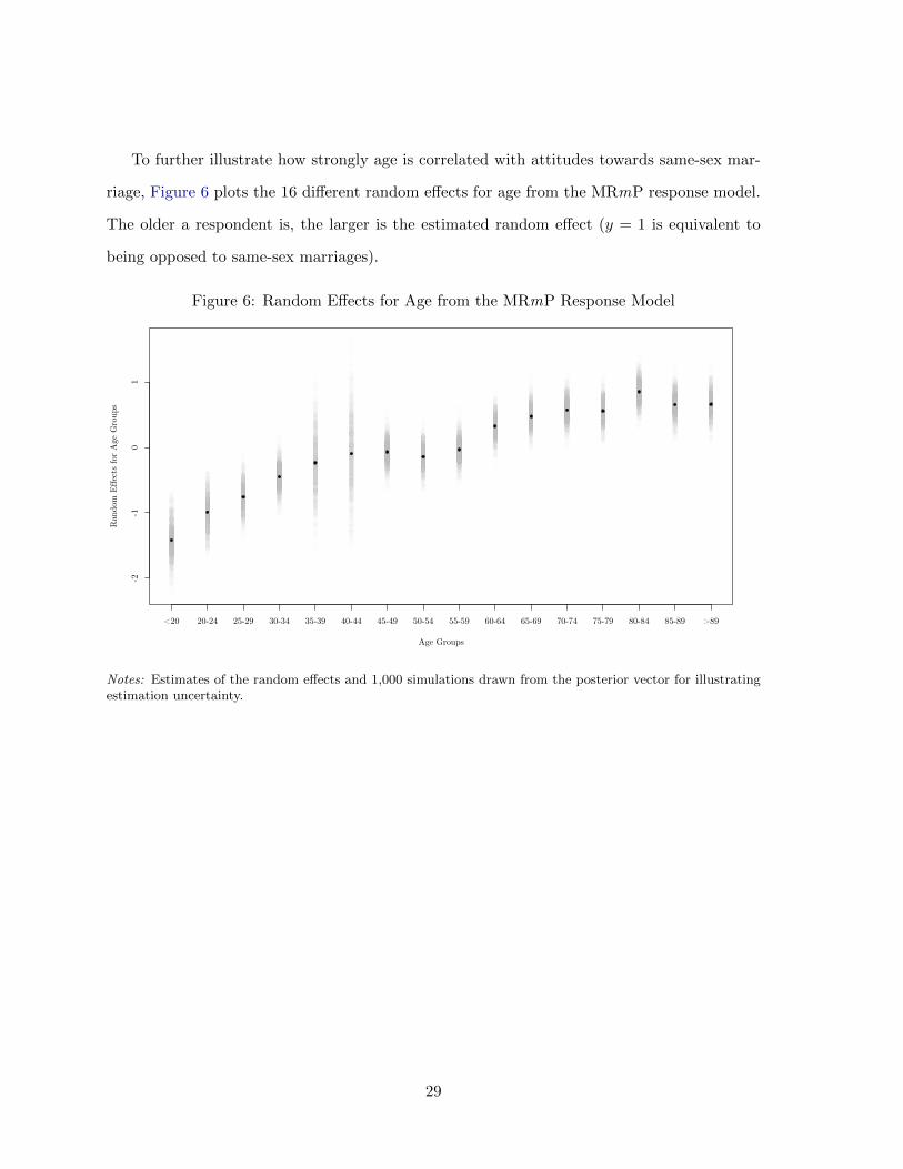
To further illustrate how strongly age is correlated with attitudes towards same-sex mar-

riage, Figure 6 plots the 16 different random effects for age from the MRmP response model.

The older a respondent is, the larger is the estimated random effect (y = 1 is equivalent to

being opposed to same-sex marriages).

Figure 6: Random Effects for Age from the MRmP Response Model

-2-1

01

Age Groups

Ran

dom

Effe

cts

for

Age

Gro

ups

<20 20-24 25-29 30-34 35-39 40-44 45-49 50-54 55-59 60-64 65-69 70-74 75-79 80-84 85-89 >89

Notes: Estimates of the random effects and 1,000 simulations drawn from the posterior vector for illustratingestimation uncertainty.

29