Extension and Enhancement of the Allen-Eggers … · Extension and Enhancement of the Allen-Eggers Analytic Solution for Ballistic Entry Trajectories Zachary R. Putnam and Robert

Extension and Enhancement of the Allen-Eggers

Analytic Solution for Ballistic Entry Trajectories

Zachary R. Putnam∗ and Robert D. Braun†

Georgia Institute of Technology, Atlanta, Georgia, 30332

The closed-form analytic solution to the equations of motion for ballistic entry developedby Allen and Eggers is extended and enhanced with a method of choosing an appropriateconstant flight-path angle, limits based on the equations of motion and acceptable ap-proximation error are proposed that bound the domain of applicability, and closed-formexpressions for range and time-dependency. The expression developed for range to goexhibits error that may low enough for onboard drag-modulation guidance and targetingsystems. These improvements address key weaknesses in the original approximate solution.Results show that the extended and enhanced Allen-Eggers solution provides good accu-racy across a range of ballistic coefficients entries at Earth with initial flight-path anglessteeper than -7 deg.

Nomenclature

A = aerodynamic reference area, m2

a = acceleration magnitude, Earth gCD = drag coefficientCL = lift coefficientD = qACD, drag magnitude, NE = energy over weight, mg = acceleration due to gravity, m/s2

H = atmospheric scale height, mh = altitude, mk = convective stagnation-point heat rate constant, kg1/2m−1

L = qACL, lift magnitude, NL/D = lift-to-drag ratiom = mass, kgq = (1/2)ρV 2, dynamic pressure, N/m2

Q = convective stagnation-point heat rate, W/cm2

R = planetary radius, mrn = effective nose radius, mS = range, mStogo = range to go, mt = time, sV = velocity magnitude, m/sVC = circular velocity, m/sW = mg, weight magnitude, Nγ = Euler’s constantβ = m/(CDA), ballistic coefficient, kg/m2

δq = initial dynamic pressure stand-off factorδV = final velocity stand-off factor

∗Graduate Research Assistant, School of Aerospace Engineering, 270 Ferst Dr., Senior Member AIAA.†Professor, School of Aerospace Engineering, 270 Ferst Dr., Fellow AIAA

1 of 27

American Institute of Aeronautics and Astronautics

Dow

nloa

ded

by G

EO

RG

IA I

NST

OF

TE

CH

NO

LO

GY

on

June

19,

201

4 | h

ttp://

arc.

aiaa

.org

| D

OI:

10.

2514

/6.2

014-

2381

AIAA Atmospheric Flight Mechanics Conference

16-20 June 2014, Atlanta, GA

AIAA 2014-2381

AIAA Aviation

γ = flight-path angle, positive above local horizontal, radγ∗ = Allen-Eggers constant flight-path angle, radρ = atmospheric density, kg/m3

θ = range angle, rad

I. Introduction

When planetary entry was first studied in the middle of the twentieth century, analytic approximationswere developed to enable vehicle and mission designers to evaluate vehicle trajectories and performance

with minimal or no computer usage. Seminal examples of these approximations include, in chronologicalorder, Sanger’s expressions for lifting entry,1 the Allen-Eggers approximation for ballistic entry,2 Chapman’sZ-function,3 Loh’s “second-order” approximation,4 and those developed by Vinh et al.5 These analytic andhybrid analytic-numeric approximate solutions utilized assumptions to make the nonlinear equations ofmotion soluble. As a result, they typically only applied to limited classes of entry vehicles and trajectories.

Advances in computing eventually made high-accuracy numeric integration of the equations of motionfeasible for most applications.6 Today, vehicle and mission designers have significant computational resourcesavailable, enabling relatively rapid, low-cost, and high-fidelity assessment of entry trajectories. However,approximate solutions are still desirable for some applications when simplicity and execution speed areparamount, such as real-time guidance, navigation, and control systems; optimization; and conceptual design.Analytic solutions also provide more information about classes of trajectories: they may be manipulated todetermine parameter sensitivities and partial derivatives. It is with these applications in mind that this studyseeks to extend and enhance the Allen-Eggers approximate solution for ballistic entry through developmentof a method for computing the assumed constant flight-path angle, bounds for the domain of applicability,and closed-form expressions for trajectory range and time.

Harry “Harvey” Julian Allen and Alfred J. Eggers, working at the Ames Aeronautical Laboratory, firstdocumented their approximate solution for ballistic (nonlifting) entry in a classified NACA research mem-orandum in 1953.7 This memorandum was declassified in 1957,7 and subsequently republished as a NACAreport in 1958.2 The primary goal of Allen’s and Eggers’ work was “to determine means available to the de-signer for minimizing aerodynamic heating” for missile applications.2 The Allen-Eggers approximate solutionis based on the insight that, for ballistic entry at a sufficiently steep initial flight-path angle, the gravitationalforce may be neglected because its magnitude is small relative to the magnitude of the drag force.2 Thisyields a closed-form analytic relationship between velocity and altitude from which Allen and Eggers wereable to derive closed-form analytic expressions for deceleration and heating, including state values at peakconditions of interest. The solution is composed of relatively simple, explicit analytic expressions.

II. Methods and Assumptions

A. Planar Equations of Motion

The hypersonic phase of planetary entry is typically unpowered; thrust is used only for attitude control, ifat all. The small amount of thrust required for attitude control results in a nearly constant vehicle mass.The scalar, planar equations of motion may be derived by considering the coordinate systems and free-bodydiagram for a planar entry trajectory shown in Fig. 1.8 The coordinate frames are the inertial frame (XI , ZI),the local horizontal frame (XL, ZL), and the wind frame (XW , ZW ). Expressing the vectors in Fig. 1 in thewind frame, one can use Newton’s second law to write two scalar equations of motion:

dV

dt= −D

m− W

gsin(γ) (1a)

dγ

dt=dθ

dt+

1

V

L

m− W

gVcos(γ) (1b)

2 of 27


Dow

nloa

ded

by G

EO

RG

IA I

NST

OF

TE

CH

NO

LO

GY

on

June

19,

201

4 | h

ttp://

arc.

aiaa

.org

| D

OI:

10.

2514

/6.2

014-

2381

From kinematics, two more equations may be written for altitude above the planetary surface and rangeangle, assuming a spherical planetary surface:

dh

dt= V sin γ (2a)

dθ

dt=V cos(γ)

h+R(2b)

The acceleration due to gravity changes little during entry, as altitude changes are one to two orders ofmagnitude less than planetary radii for most applications. Therefore, g is assumed to be constant duringentry. Atmospheric density is assumed to vary exponentially with altitude according to:

ρ = ρref exp

(href − h

H

)(3)

While the scale height varies with altitude in a real atmosphere, the most interesting aspects of planetaryentry, such as peak deceleration and peak heating, occur in a relatively narrow altitude band, making theassumption of constant scale height reasonable with appropriate selection of ρref and href . The referencedensity need not be selected as the zero-altitude density; choosing ρref and H associated with a higheraltitude may produce a more accurate representation of the true atmospheric density profile over the altituderange of interest.

The equations of motion can be simplified by assuming constant values for the aerodynamic coefficientsand thus for β and L/D. While the aerodynamic properties of an entry vehicle generally vary with Machnumber and angle-of-attack to first order, Mach-number independence in the hypersonic flight regime (Machnumbers above about 5) makes constant aerodynamic coefficients a good assumption for most planetaryentry trajectories.9

+XI

+ZI

+XL +ZL

+XW

+ZW local

horizontal

planetary surface

O +XI

-ZI

r

V

γ

θ

L D

W

θ

equatorial plane

pola

r axi

s

h

R

Figure 1. Coordinate systems and free-body diagram for a planar planetary entry trajectory.

Combining Eqs. (1) through (3) and rearranging terms, the planar equations of motion for a planetaryentry vehicle may be written as:

dV

dt= −

[ρref2β

exp

(href − h

H

)]V 2 − g sin(γ) (4a)

dγ

dt=V cos γ

R+ h+

[ρref2β

exp

(href − h

H

)](L

D

)V − g

Vcos(γ) (4b)

dh

dt= V sin(γ) (4c)

dθ

dt=V cos γ

R+ h(4d)

3 of 27


Dow

nloa

ded

by G

EO

RG

IA I

NST

OF

TE

CH

NO

LO

GY

on

June

19,

201

4 | h

ttp://

arc.

aiaa

.org

| D

OI:

10.

2514

/6.2

014-

2381

Eqs. (4) are a set of coupled, first-order, ordinary differential equations. These equations are highly nonlineardue to the presence of the planetary atmosphere and defy analytic solution unless simplifying assumptionsare applied.

B. Computational Methods

In this study, approximation errors generally are presented as a percentage relative to Eqs. (4). Eqs. (4)are solved numerically using Matlab’s intrinsic ode45 function with absolute and relative error tolerancesof 10−12. Error presented as absolute error is the absolute value of the error magnitude. The normalizedintegrated error is used to compare approximation error across multiple trajectories and is defined by:

εX =1

εX,norm

√√√√ N∑i=1

(Xi,approx −Xi,EOM

Xi,EOM

)2

(5)

where N is the total number of points computed for the trajectory and X represents the trajectory state ofinterest. While individual values of this integrated error are physically meaningless, they provide an estimateof the efficacy of an approximate solution relative to a known trajectory. The Mathematica computer algebrasystem was used to symbolically evaluate the complex integrals in this study.

C. Example Entry Trajectories

Three example trajectories were chosen to illustrate the extension and enhancement of the Allen-Eggersapproximate solution: interplanetary robotic sample return, strategic reentry, and low-Earth orbit (LEO)return of crew from the International Space Station. These example trajectories span a range of initialconditions and vehicle parameters and represent current ballistic entry missions of interest at Earth to theentry community (see Table 1). The sample-return example is based on NASA’s Stardust Sample ReturnCapsule, which successfully landed after a ballistic entry in 2006.10 Stardust had the greatest initial velocityof any Earth-return mission. The strategic example features a high ballistic coefficient vehicle on a steep,high-energy suborbital trajectory.11 The LEO-return example represents ballistic entry of a crewed vehicleand is based on data from the off-nominal ballistic entry of Soyuz TMA-11.13 This example is consistentwith other blunt-body crewed entry systems and enters the atmosphere at a very shallow flight-path angle.Together, these examples include hyperbolic, orbital, and suborbital entry energies and span several ordersof magnitude of ballistic coefficient.

Table 1. Parameters for Example Trajectories at Earth

Parameter Sample Return10,12 Strategic11 LEO Return13

Equatorial radius, R 6378.0 km 6378.0 km 6378.0 km

Gravitational acceleration, g 9.81 m/s2 9.81 m/s2 9.81 m/s2

Atmospheric scale height, H 8.5 km 8.5 km 8.5 km

Reference atmospheric density, ρref 1.215 kg/m3 1.215 kg/m3 1.215 kg/m3

Reference altitude, href 0 km 0 km 0 km

Initial velocity, V0 12.8 km/s 7.2 km/s 7.9 km/s

Initial flight-path angle, γ0 -8.2 deg -30.0 deg -1.35 deg

Initial altitude, h0 125 km 125 km 100 km

Ballistic coefficient, β 60 kg/m2 10000 kg/m2 450 kg/m2

Lift-to-drag ratio, L/D 0 0 0

III. Review and Modernization of the Allen-Eggers Solution

The Allen-Eggers solution is rederived below using modern nomenclature. The results differ slightly fromthose presented in Ref. 2 due to use of the current convention for the definition of flight-path angle andballistic coefficient. A more general atmosphere model including a reference altitude is also used.

4 of 27


Dow

nloa

ded

by G

EO

RG

IA I

NST

OF

TE

CH

NO

LO

GY

on

June

19,

201

4 | h

ttp://

arc.

aiaa

.org

| D

OI:

10.

2514

/6.2

014-

2381

A. Altitude-Velocity Profile

The Allen-Eggers altitude-velocity profile may be derived by recognizing that for sufficiently steep entries thedrag force magnitude is much greater than the gravity force magnitude. Eqs. (4) are well-suited for modelingballistic entry, because ballistic vehicles have no out-of-plane control authority. Starting from Eq. (4a) andneglecting the gravity term relative to the drag term, one may write:

dV

dt= −ρref

2βexp

(href − h

H

)V 2 (6)

Rearranging Eq. (4c) yields:

V =1

sin γ

dh

dt(7)

Substituting Eq. (7) into Eq. (6) and separating variables gives:

1

V

dV

dt= − ρref

2β sin γexp

(href − h

H

)dh

dt(8)

Assuming a constant flight-path angle γ∗ and eliminating dt, this expression can be integrated from somestate 1 to some state 2 and solved for V2:

V2 = V1 exp

{Hρref

2β sin γ∗

[exp

(href − h2

H

)− exp

(href − h1

H

)]}(9)

This expression, first derived by Allen and Eggers, determines an altitude-velocity profile (h2, V2) as afunction of the planetary atmosphere (ρref , href , H), vehicle properties (β), and a reference vehicle state(V1, h1, γ1 = γ∗). Allen and Eggers suggest using the initial flight-path angle for γ∗;2 this approach workswell for the steep entry trajectories (γ0 � 0) that were of interest to Allen and Eggers. Lastly, Eq. (9)assumes that velocity is monotonically decreasing with altitude, limiting application of this approximatesolution to trajectories with no positive altitude rate.

B. Acceleration Magnitude

Combining Eqs. (6) and (9) results in an equation for the acceleration magnitude. This expression, normalizedby g, is given by:

a2 = −dV/dtg

∣∣∣∣2

=ρref2βg

V 21 exp

(href − h2

H

)exp

{Hρrefβ sin γ∗

[exp

(href − h2

H

)− exp

(href − h1

H

)]}(10)

Eq. (10) yields a relatively simple expression for the altitude at peak deceleration:

hamax= href +H ln

(− Hρrefβ sin γ∗

)(11)

Combining Eq. (11) and Eq. (9), the velocity at peak deceleration is:

Vamax =V1√e

exp

[− Hρref

2β sin γ∗exp

(href − h1

H

)](12)

The maximum acceleration is given by:

amax = − sin γ∗

2egHV 21 exp

[− Hρrefβ sin γ∗

exp

(href − h1

H

)](13)

If hamaxis below the planetary surface, peak deceleration occurs at minimum altitude hmin and is given by:

amax =ρref2βg

V 21 exp

(href − hmin

H

)exp

{Hρrefβ sin γ∗

[exp

(href − hmin

H

)− exp

(href − h1

H

)]}(14)

where the velocity is:

Vamax= V1 exp

{Hρref

2β sin γ∗

[exp

(href − hmin

H

)− exp

(href − h1

H

)]}(15)

5 of 27


Dow

nloa

ded

by G

EO

RG

IA I

NST

OF

TE

CH

NO

LO

GY

on

June

19,

201

4 | h

ttp://

arc.

aiaa

.org

| D

OI:

10.

2514

/6.2

014-

2381

C. Convective Heat Rate

Allen and Eggers formulated an equation for the convective heat rate at the stagnation point of a blunt-bodyvehicle:2

Q = k

√ρ

rnV 3 (16)

This equation assumes that the vehicle is sufficiently blunt such that a detached bow shock exists aheadof the body. Blunt leading edges for hypersonic vehicles are an innovation developed by Allen as a way toreduce the severity of entry heating on the vehicle.14 In Allen’s and Eggers’ original document, k is givena value of 6.8× 10−6 without units;2 dimensional analysis indicates k has units of kg1/2m−1. A value for ksuitable for application at Earth was computed using the method developed by Sutton and Graves.15

Combining Eq. (16) and Eq. (9) results in an expression for heat rate as a function of altitude:

Q2 = k

√ρrefrn

V 31 exp

(href − h2

2H

)exp

{3Hρref2β sin γ∗

[exp

(href − h2

H

)− exp

(href − h1

H

)]}(17)

The altitude and velocity at maximum heat rate are given by:

hQmax= href +H ln

(−3Hρrefβ sin γ∗

)(18)

VQmax=

V1e1/6

exp

[− Hρref

2β sin γ∗exp

(href − h1

H

)](19)

The maximum heat rate is (for hQmax≥ hmin):

Qmax = k

√−β sin γ∗

3eHrnV 31 exp

[− 3Hρref

2β sin γ∗exp

(href − h1

H

)](20)

Otherwise, the maximum heat rate occurs at the minimum altitude (h = hmin) and the peak heat rate isgiven by:

Qmax = k

√ρrefrn

V 31 exp

(href − hmin

2H

)exp

{3Hρref2β sin γ∗

[exp

(href − hmin

H

)− exp

(href − h1

H

)]}(21)

The velocity at this condition is given by Eq. (15).

D. Simplified Expressions

Setting href to 0 m, state 2 to the current state (without subscript), and state 1 to the initial vehicle statenear the top of the atmosphere (designated by the subscript 0) such that exp [−h/H] � exp [−h0/H], asimpler expression for the altitude-velocity profile results:

V = V0 exp

[Hρref

2β sin γ∗exp

(− h

H

)](22)

where ρref is now the density at zero altitude. These assumptions also simplify the expressions for acceler-ation and the conditions at maximum acceleration. Eq. (10) becomes:

a =ρref2βg

V 20 exp

(− h

H

)exp

[Hρrefβ sin γ∗

exp

(− h

H

)](23)

The conditions at peak acceleration are then given by (for hamax> hmin):

hamax= H ln

(− Hρrefβ sin γ∗

)(24)

Vamax=

V0√e≈ (0.6065)V0 (25)

6 of 27


Dow

nloa

ded

by G

EO

RG

IA I

NST

OF

TE

CH

NO

LO

GY

on

June

19,

201

4 | h

ttp://

arc.

aiaa

.org

| D

OI:

10.

2514

/6.2

014-

2381

amax = − sin γ∗

2egHV 20 (26)

The expression for heat rate becomes:

Q = k

√ρrefrn

V 30 exp

(− h

2H

)exp

[3Hρref2β sin γ∗

exp

(− h

H

)](27)

The conditions at peak heat rate are then (for hQmax> hmin):

hQmax= H ln

(−3Hρrefβ sin γ∗

)(28)

VQmax=

V0e1/6

≈ (0.8465)V0 (29)

Qmax = k

√−β sin γ∗

3eHrnV 30 (30)

These simplified expressions are closer in form to those originally presented by Allen and Eggers.2 Theyalso provide insight into several phenomena. First, the altitudes at which maximum acceleration and heat rateoccur are not functions of velocity: they are dictated entirely by vehicle parameters, planetary parameters,and the flight-path angle. In contrast, the velocities at maximum acceleration and heat rate are fractionsof the initial velocity only, and peak heating always occurs prior to peak deceleration. Lastly, as one mightexpect, maximum acceleration and heat rate are driven primarily by the initial velocity of the vehicle: greaterinitial kinetic energies result in greater values of acceleration and heat rate.

E. Example Applications

Figure 2 shows example applications of the modernized Allen-Eggers approximate solution to the threeplanetary entry trajectories specified in Table 1. The approximate trajectories are co-plotted with numericsolutions to Eqs. (4). Error plots are provided in Fig. 3. The Allen-Eggers approximation shows goodagreement with the planar equations of motion for the strategic case. The altitude (Fig. 2a) and heat-rateprofiles (Fig. 2d) show small approximation errors for the sample-return case, but the acceleration error isnearly 50%. The Allen-Eggers solution does a poor job approximating the shallow LEO-return case.

The assumptions used in the derivation of the Allen-Eggers solution lead to the smallest error during thehypersonic portion of the trajectory. This regime encompasses the acceleration and heating pulses, includingpeak values for these quantities. These quantities and qualities of a planetary entry trajectory typically driveentry vehicle and mission design, making the Allen-Eggers approximate solution a useful tool for conceptualmission and vehicle design and analysis. Values of vehicle states at peak acceleration and peak heat rateestimated by the Allen-Eggers approximation are given in Tables 2 and 3, respectively. As before, errorsfor the strategic example are uniformly low. Estimates of conditions at peak heat rate are within 20% forboth the sample-return and LEO-return cases; estimation error for peak acceleration is significantly largerfor these cases. Reducing in this error will make Allen-Eggers approximation applicable for estimating statesat peak conditions for more mission classes.

The nature of the error in Fig. 3 points towards several weaknesses in the solution. First, while choosingthe initial flight-path angle appears to be a good choice for γ∗ for the strategic case, this is not true for theother cases. Second, development of bounds on the domain of applicability on the solution would providethe user with greater confidence in the approximation without direct comparison with numeric solutions.Lastly, the Allen-Eggers solution does not provide any information on range or time of flight for entry, bothof which are useful quantities for onboard guidance and targeting systems.

IV. Extensions and Enhancements to the Allen-Eggers Solution

Several extensions and enhancements to the Allen-Eggers approximate solution are proposed to addressimplementation weaknesses, provide additional information, and extend applicability of the solution: amethod for computing the constant flight-path angle, bounds on the domain of applicability, closed-form

7 of 27


Dow

nloa

ded

by G

EO

RG

IA I

NST

OF

TE

CH

NO

LO

GY

on

June

19,

201

4 | h

ttp://

arc.

aiaa

.org

| D

OI:

10.

2514

/6.2

014-

2381

0 5 100

50

100Al

titud

e, k

m

Velocity, km/s0 5 10 15

0

20

40

60

Acce

lera

tion,

Ear

th g

Velocity, km/s

0 5 10 15−40

−30

−20

−10

0

Flig

ht−p

ath

angl

e, d

eg


100

102

104

Hea

t rat

e, W

/cm

2

Velocity, km/s

a)

c) d)

b)

Sample return Strategic LEO return Numeric int. of Eqs. (4)

Figure 2. Example application of the Allen-Eggers approximate solution: a) altitude, b) acceleration, c)flight-path angle, and d) heat rate versus velocity.

Table 2. Vehicle States at Peak Acceleration

Acceleration Velocity Altitude

Value, g Error, % Value, km/s Error, % Value, km Error, %

Sample return 50.0 34.9 7.64 -2.1 60.3 -4.6

Strategic 57.2 -5.1 4.37 -1.8 6.2 3.6

LEO return 3.3 -57.3 4.81 34.9 58.5 27.0

Table 3. Vehicle States at Peak Heat Rate

Heat rate Velocity Altitude

Value, W/cm2 Error, % Value, km/s Error, % Value, km Error, %

Sample return 391.5 12.3 10.67 -1.2 69.7 -3.6

Strategic 1764.3 -6.5 6.09 -1.8 15.5 1.3

LEO return 108.5 -18.0 6.71 4.7 67.8 9.2

8 of 27


Dow

nloa

ded

by G

EO

RG

IA I

NST

OF

TE

CH

NO

LO

GY

on

June

19,

201

4 | h

ttp://

arc.

aiaa

.org

| D

OI:

10.

2514

/6.2

014-

2381

0 5 10−100

−50

0

50

100

Altit

ude

erro

r, %

Velocity, km/s0 5 10

−100

−50

0

50

100

Acce

lera

tion

erro

r, %

Velocity, km/s

0 5 10−100

−50

0

50

100

Flig

ht−p

ath

angl

e er

ror,

%


−100

−50

0

50

100

Hea

t rat

e er

ror,

%

Velocity, km/s

a)

c) d)

b)

Sample return Strategic LEO return

Figure 3. Allen-Eggers approximation error for a) altitude, b) acceleration, c) flight-path angle, and d) heatrate versus velocity.

9 of 27


Dow

nloa

ded

by G

EO

RG

IA I

NST

OF

TE

CH

NO

LO

GY

on

June

19,

201

4 | h

ttp://

arc.

aiaa

.org

| D

OI:

10.

2514

/6.2

014-

2381

expressions for range, and formulation of the approximation as a function of time. In an effort to maintainthe character of the Allen-Eggers solution, these developments result in explicit, analytic, and relativelysimple expressions.

A. Determining the Constant Flight-Path Angle

A singular issue when applying the Allen-Eggers approximate solution to a real-world problem is determininga proper value for γ∗, the assumed constant flight-path angle. Steep entries exhibit only a small change inflight-path angle from its initial value in the hypersonic regime, making γ0 a good approximation of γ∗;shallow trajectories fly at near-constant flight-path angles that are significantly different from the initialvalue, making γ0 a relatively poor choice for γ∗. The ability to accurately determine more appropriatevalues for γ∗ will extend the domain of applicability of the Allen-Eggers approximate solution to moreshallow initial flight-path angles and improve overall accuracy.

1. Determining γ∗

It is desirable to develop a method for determining γ∗ based on available information that that is closed-form, explicit, and does not require numeric integration to preserve the advantages of the Allen-Eggerssolution. The solution for flight-path angle as a function of velocity developed by Citron and Meir meetsthese criteria.16 Other approximate solutions for flight-path angle were considered: Loh’s “Second-order”solution,4 Yaroshevskiy’s series approximation,17,18 and Chapman’s z-function solution.3 However, nonewere explicit, analytic, and generally-applicable.

The Citron-Meir expression for flight-path angle is, rederived to be consistent with nomenclature definedin this study and with L/D = 0:

sin γ = sin γ0 (2F − 1) (31)

where

F =

[1 +

H

R tan2 γ0

{V 2C

V 20

[Ei

(lnV 20

V 2

)− γ − ln

(lnV 20

V 2

)]+

(V 2C

V 20

− 1

)ln

(1− β sin γ0

Hρ0lnV 20

V 2

)}]1/2(31a)

where ρ0 is the density at V0 and Ei is the exponential integral, defined by:

Ei(x) = −∫ ∞−x

exp (−y)

ydy (32)

The exponential integral may be approximated using the explicit, analytic method developed by Cody andThacher.19 Given an initial state, planetary properties, and ballistic coefficient, Eq. (31) determines theflight-path angle as a function of velocity for most non-skipping entry trajectories.16

Comparing Fig. 2b and c with Fig. 4, the value of the flight-path angle near peak acceleration appears tobe a better representation of the constant flight-path angle γ∗ than the initial flight-path angle. The velocityat this condition, V ∗ = Vamax

, can be found using existing relationships in the Allen-Eggers solution; V ∗ maythen be used in Eq. 31 to determine γ∗. Either Allen-Eggers expression for Vamax may be used to determineV ∗: Eq. (12) or the simplified expression, Eq. (25). Using the simplified expression for Vamax yields a morecompact expression for γ∗. Substituting Eq. (25) into Eq. (31) gives:

sin γ∗ = sin γ0 (2F − 1) (33)

where

F =

[1 +

H

R tan2 γ0

{CV 2C

V 20

+

(V 2C

V 20

− 1

)ln

(1− β sin γ0

Hρ0

)}]1/2(33a)

andC = Ei(1)− γ ≈ 1.3179 (33b)

The constant C need only be determined once to the desired accuracy. As such, this expression does notrequire repeated evaluation of the exponential integral.

Figure 4 shows the efficacy of the proposed method for estimating γ∗ for the sample-return trajectory atdifferent initial flight-path angles. The resulting values for γ∗ more closely approximate numeric solutions of

10 of 27


Dow

nloa

ded

by G

EO

RG

IA I

NST

OF

TE

CH

NO

LO

GY

on

June

19,

201

4 | h

ttp://

arc.

aiaa

.org

| D

OI:

10.

2514

/6.2

014-

2381

flight-path angle as a function of velocity. The difference between the proposed method and using γ0 for γ∗

increases with more shallow initial flight-path angles, but improvement is present for all initial flight-pathangles shown. Both options for computing V ∗ are shown; the additional complexity of using Eq. (12) withEq. (31) does not yield results that are appreciably different from those generated by Eq. (33).

0 5 10 15−50

−40

−30

−20

−10

0

Flig

ht−p

ath

angl

e, d

eg

Velocity, km/s

γ0 = -40 deg

γ0 = -30 deg

γ0 = -20 deg

γ0 = -10 deg γ0 = -6 deg

V* = Eq. (26) V* = Eq. (13) V* = V0 (γ* = γ0) Numeric int. of Eqs. (4)

Figure 4. The proposed method for determining γ∗ more closely approximates the flight-path angle as afunction of velocity than setting γ∗ = γ0.

2. Improvements to Approximation Accuracy

The proposed method for determining γ∗ improves the accuracy of the Allen-Eggers approximate solutionacross all three example cases (Fig. 5 and Fig. 6). The improvement is most significant for the sample-returnexample: deceleration and flight-path angle estimation error is reduced by nearly 40% near mid-trajectory.For the LEO-return case, error is reduced and more balanced about zero, but remains large. Improvementsto the strategic case are small.

As shown in Fig. 6, estimates of vehicle states at peak acceleration and heat rate are improved for allthree cases with the exception of the peak heat rate for the LEO-return case. This increase in error isaccompanied by an equally large decrease in the error for the estimate of the peak deceleration, as well assmaller reductions in error for estimates of the velocity and altitude at these conditions.

B. Bounding the Domain of Applicability

Figure 7 shows the Allen-Eggers approximate altitude-velocity profile relative to the numeric solution to theequations of motion early and late in the trajectory as a function of the normalized velocity. Early in thetrajectory (Fig. 7b), the Allen-Eggers approximation is invalid because vehicle dynamics are dominated bygravity, which is explicitly neglected. At high altitudes, atmospheric density is low, and therefore drag islow, and gravity dominates, causing the vehicle to accelerate as it descends into the planetary gravity well.As vehicle altitude decreases, atmospheric density builds, causing drag to increase and surpass gravity asthe dominate force, causing the vehicle to decelerate. There is a point at which the drag and gravity forcesare balanced: above this point, gravity dominates; below, drag dominates. The Allen-Eggers approximationbecomes much more accurate once drag dominates the dynamics.

Late in the trajectory, the Allen-Eggers approximation error becomes large again (Fig. 7a). After passingthrough peak deceleration vehicle velocity continues to decrease, decreasing dynamic pressure and the dragforce. Eventually, the drag force decreases enough that gravity becomes significant again, causing a negativeflight-path angle rate known as the gravity turn. In this region of the trajectory, the Allen-Eggers assumptionson gravity and constant flight-path angle are both violated.

While the Allen-Eggers approximate solution shows significant error early and late in the example tra-jectory where its underlying assumptions are invalid, it is accurate for the middle of entry trajectories,encompassing the hypersonic regime. The direct link between the inaccuracies in the Allen-Eggers approxi-mate solution early and late in the trajectory and the approximation’s underlying assumptions suggest thata bounded domain can be identified, based on the equations of motion, over which the approximate solutionis valid.

11 of 27


Dow

nloa

ded

by G

EO

RG

IA I

NST

OF

TE

CH

NO

LO

GY

on

June

19,

201

4 | h

ttp://

arc.

aiaa

.org

| D

OI:

10.

2514

/6.2

014-

2381

0 5 10−100

−50

0

50

100Al

titud

e er

ror,

%


−100

−50

0

50

100

Acce

lera

tion

erro

r, %

Velocity, km/s

0 5 10−100

−50

0

50

100

Flig

ht−p

ath

angl

e er

ror,

%


−100

−50

0

50

100

Hea

t rat

e er

ror,

%

Velocity, km/s

γ* = γ0 Proposed method for computing γ*

a)

c) d)

b)


Figure 5. Approximation error with and without the proposed method for computing γ∗.

0

10

20

30

40

50

60

Abso

lute

erro

r, %

Vamax hamax VQmax hQmax Qmax amax

γ* = γ0 V* = V0 Sample return Strategic LEO return

γ* = Eq. (32) V* = Eq. (24) Sample return Strategic LEO return

Figure 6. Vehicle states at peak conditions for γ∗ = γ0 and the proposed method of estimating γ∗.

12 of 27


Dow

nloa

ded

by G

EO

RG

IA I

NST

OF

TE

CH

NO

LO

GY

on

June

19,

201

4 | h

ttp://

arc.

aiaa

.org

| D

OI:

10.

2514

/6.2

014-

2381

0 0.1 0.2 0.3 0.4 0.5

0

20

40

60

Altit

ude,

km

Normalized velocity, V/V0

0.99 0.995 1 1.005 1.01 1.015

40

60

80

100

120

Altit

ude,

km

Normalized velocity, V/V0a) b)


Figure 7. Allen-Eggers approximation error in altitude-velocity profile a) late and b) early in trajectory.

1. Bound on Minimum Velocity

A minimum-velocity bound on the domain of applicability for the Allen-Eggers approximate solution maybe derived by considering Eq. (4b) for ballistic vehicles, rearranged:

dγ

dt=

(V

R+ h− g

V

)cos γ (34)

As shown in Figs. 2c and 7a, the Allen-Eggers approximate solution becomes inaccurate when the flight-pathangle begins to change significantly, indicating a nonzero (and negative) value of dγ/dt. Since cos γ tendsto decrease with increasingly negative γ, any significant increase in the magnitude of dγ/dt must be causedby an increase in the magnitude of the other factor. Since larger values of dγ/dt occur late in the trajectoryand the sign of dγ/dt is negative, one can say that a significant dγ/dt results when the gravity term, g/V , islarger than the range-rate term, V/(R+ h), by some factor, δ2, and the Allen-Eggers approximation is onlyvalid for velocities above that point:

δ2( gV

)>

V

R+ h(35)

Neglecting h relative to R (a good assumption at low altitudes near the end of the trajectory) and solvingfor V determines a lower limit on velocity past which the gravity term exceeds the range-rate term by thefactor δ2:

V >√δ2gR (36)

Defining the minimum acceptable final velocity as Vf , rearranging, and designating δ as δV , one finds theminimum final velocity is:

Vf = δV√gR = δV VC (37)

This shows that Vf is merely a faction of the circular velocity, the velocity of a notional circular orbit at theplanetary surface, and δV is a stand-off parameter that relates the lower bound of the Allen-Eggers velocitydomain to planetary parameters. Figure 8 shows the minimum velocity for three values of δV . Larger valuesof δV imply a more restrictive domain for the Allen-Eggers approximation.

An appropriate value of δV may be chosen by examining the Allen-Eggers approximation error as afunction of δV , as shown in Fig. 9a for the sample-return example trajectory. The figure indicates that aδV of 0.05 will limit approximation error in altitude, deceleration, and heat rate to less than approximately20%. While the flight-path angle error remains large at this value of δV , the Allen-Eggers solution does notattempt to estimate the flight-path angle, making this error less significant.

2. Bound on Initial Dynamic Pressure

A bound on the initial state may also be derived to complete the specification of the domain of applicabilityfor the Allen-Eggers approximation. Figure 7b shows that the Allen-Eggers approximation is inaccurate in

13 of 27


Dow

nloa

ded

by G

EO

RG

IA I

NST

OF

TE

CH

NO

LO

GY

on

June

19,

201

4 | h

ttp://

arc.

aiaa

.org

| D

OI:

10.

2514

/6.2

014-

2381

0 2 4 6 8 10 12 140

20

40

60

80

100

120

Velocity, km/s

Altit

ude,

km

δq = 1

δq = 5 δq = 10

δ v =

0.0

1

δ v =

0.1

δ v =

0.2

Numeric int. of Eqs. (4): Sample return

Figure 8. Example bounds on the Allen-Eggers domain of applicability for the sample-return example casefor several values of δV and δq.

0 0.05 0.1 0.15 0.2 0.25−100

−50

0

50

100

bV, nd

Erro

r, %

AltitudeFlight−path angleAccelerationHeat rate

2 4 6 8 1010−1

100

101

102

103

bq, nd

Abso

lute

erro

r, %

a) b)

V = V0

V = 95% V0

Figure 9. Allen-Eggers approximation error versus a) the final velocity stand-off factor δV and b) the initialdynamic pressure stand-off factor δq.

14 of 27


Dow

nloa

ded

by G

EO

RG

IA I

NST

OF

TE

CH

NO

LO

GY

on

June

19,

201

4 | h

ttp://

arc.

aiaa

.org

| D

OI:

10.

2514

/6.2

014-

2381

the region when velocity is increasing under the influence of gravity. The point at which the gravity anddrag forces balance occurs when velocity is at a maximum. At this point, from Eq. (4a):

dV

dt= 0 = − ρ

2βV 2 − g sin γ (38)

The Allen-Eggers approximation assumes the gravity force is negligible relative to the drag force, or:

ρ

2βV 2 � −g sin γ (39)

where γ < 0 for entry, making the right-hand side positive. Rearranging:

q � −gβ sin γ (40)

The limit on the initial dynamic pressure, q0, may then be defined in terms of a standoff factor, δq, and theinitial flight-path angle such that:

q0 = −δqgβ sin γ0 (41)

Eq. (41) defines a limit on the initial dynamic pressure, and therefore on the acceptable set of (V0, h0),as a function of the initial flight-path angle, vehicle properties, planetary properties, and the stand-off factorδq. A δq value of 1 indicates the dynamic pressure at maximum velocity. Figure 8 shows how this dynamicpressure limit leads to limits on the initial velocity and altitude for several values of δq. Conventionally, theinitial conditions for entry are defined at an arbitrary altitude; Eq. (41) defines initial conditions for entrytrajectories based on when the atmosphere begins to dominate vehicle dynamics.

Similarly to δV , an appropriate value for δq may be chosen by examining the Allen-Eggers state approx-imation error as a function of δq. Figure 9b shows approximation error for sample-return trajectory at V0and at 95% of V0 as a function of δq. States at two velocities are shown because there is no approximationerror in the altitude or flight-path angle at the initial state. Heat rate percent error is large at both points,but the magnitude of this error is small due to the high altitude and low density. A δq value of 2 is chosento provide margin relative to the maximum velocity point (δq = 1) while limiting the initial approximationerror in acceleration to 100%.

3. Improvements to Approximation Accuracy

Figures 10 and 11 show the decrease in approximation error for the example trajectories with the Allen-Eggers approximation restricted to its domain of applicability by limits on Vf and q0 with δV = 0.05 andδq = 2. Modest improvement in approximation error is apparent for the sample-return and strategic cases.No improvement is seen in the LEO-return case because its initial dynamic pressure exceeds that associatedwith a δq of 2.

C. Closed-Form Expressions for Range

Closed-form, explicit approximations for entry range have generally been restricted to vehicles with nonzeroL/D, such as equilibrium glide20 and Sanger’s steep lifting entry.1 For ballistic entry, approximate tra-jectory solutions in the literature either omit range, evaluate range through integrals that must be solvednumerically,21 or utilize highly-truncated series approximations.22 No closed-form analytic expression forballistic entry range has been identified in the current literature. Analytic solutions to the states of theequations of motion are often complex and must be combined into an additional integral to compute range.The complexity of this range integrand typically defies analytic solution.

Modern computational symbolic integration has been used to develop closed-form expressions for rangeand range to go as functions of velocity for the Allen-Eggers approximate solution. These range expressionsextend the Allen-Eggers approximate solution to cover all four states in Eqs. (4).

1. Derivation

The energy over weight for an entry vehicle is defined by:

E =1

mg

(1

2mV 2 +mgh

)=V 2

2g+ h (42)

15 of 27


Dow

nloa

ded

by G

EO

RG

IA I

NST

OF

TE

CH

NO

LO

GY

on

June

19,

201

4 | h

ttp://

arc.

aiaa

.org

| D

OI:

10.

2514

/6.2

014-

2381

0 5 10−100

−50

0

50

100Al

titud

e er

ror,

%


−100

−50

0

50

100

Acce

lera

tion

erro

r, %

Velocity, km/s

0 5 10−100

−50

0

50

100

Flig

ht−p

ath

angl

e er

ror,

%


−100

−50

0

50

100

Hea

t rat

e er

ror,

%

Velocity, km/s


Bounded

a)

c) d)

b)

Figure 10. Approximation error for bounded and unbounded domains.

0

10

20

30

40

50

60

Abso

lute

erro

r, %

Unbounded Sample return Strategic LEO return Bounded Sample return Strategic LEO return


Figure 11. Allen-Eggers approximation error of vehicle states at peak conditions for bounded and unboundeddomains.

16 of 27


Dow

nloa

ded

by G

EO

RG

IA I

NST

OF

TE

CH

NO

LO

GY

on

June

19,

201

4 | h

ttp://

arc.

aiaa

.org

| D

OI:

10.

2514

/6.2

014-

2381

The derivative of the energy over weight with respect to time is given by, substituting in Eqs. (4a) and (4c):

dE

dt=V

g

dV

dt+dh

dt= − ρ

2gβV 3 (43)

The derivative of the subtended range angle with respect to the energy over weight is then:

dθ

dE=

dθ/dt

dE/dt=−2βg cos γ

ρV 2(R+ h)(44)

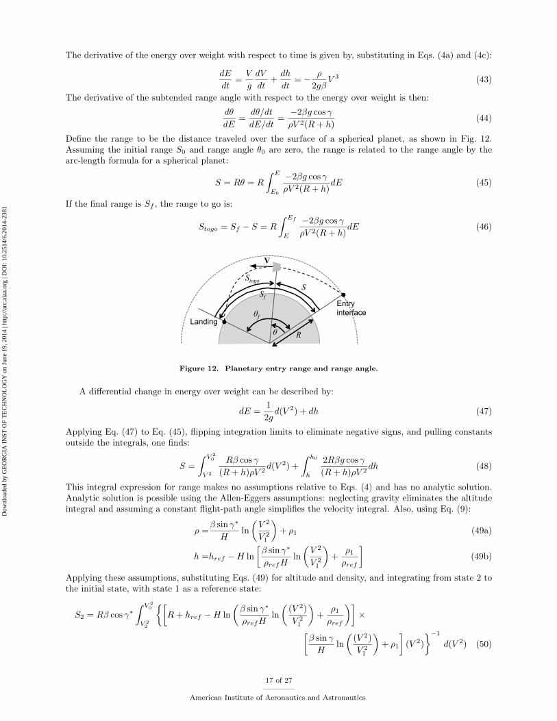
Define the range to be the distance traveled over the surface of a spherical planet, as shown in Fig. 12.Assuming the initial range S0 and range angle θ0 are zero, the range is related to the range angle by thearc-length formula for a spherical planet:

S = Rθ = R

∫ E

E0

−2βg cos γ

ρV 2(R+ h)dE (45)

If the final range is Sf , the range to go is:

Stogo = Sf − S = R

∫ Ef

E

−2βg cos γ

ρV 2(R+ h)dE (46)

S Stogo

Entry interface

Landing

Sf

V

θf

θ R

Figure 12. Planetary entry range and range angle.

A differential change in energy over weight can be described by:

dE =1

2gd(V 2) + dh (47)

Applying Eq. (47) to Eq. (45), flipping integration limits to eliminate negative signs, and pulling constantsoutside the integrals, one finds:

S =

∫ V 20

V 2

Rβ cos γ

(R+ h)ρV 2d(V 2) +

∫ h0

h

2Rβg cos γ

(R+ h)ρV 2dh (48)

This integral expression for range makes no assumptions relative to Eqs. (4) and has no analytic solution.Analytic solution is possible using the Allen-Eggers assumptions: neglecting gravity eliminates the altitudeintegral and assuming a constant flight-path angle simplifies the velocity integral. Also, using Eq. (9):

ρ =β sin γ∗

Hln

(V 2

V 21

)+ ρ1 (49a)

h =href −H ln

[β sin γ∗

ρrefHln

(V 2

V 21

)+

ρ1ρref

](49b)

Applying these assumptions, substituting Eqs. (49) for altitude and density, and integrating from state 2 tothe initial state, with state 1 as a reference state:

S2 = Rβ cos γ∗∫ V 2

0

V 22

{[R+ href −H ln

(β sin γ∗

ρrefHln

((V 2)

V 21

)+

ρ1ρref

)]×[

β sin γ

Hln

((V 2)

V 21

)+ ρ1

](V 2)

}−1d(V 2) (50)

17 of 27


Dow

nloa

ded

by G

EO

RG

IA I

NST

OF

TE

CH

NO

LO

GY

on

June

19,

201

4 | h

ttp://

arc.

aiaa

.org

| D

OI:

10.

2514

/6.2

014-

2381

Evaluating this integral analytically results in a closed-form solution for range as a function of velocity:

S2 = R cot γ∗(

ln

{H ln

[ρ1ρref

+β sin γ∗

Hρrefln

(V 22

V 21

)]− href −R

}−

ln

[H ln

(ρ1ρref

+β sin γ∗

Hρrefln

(V 20

V 21

))− href −R

])(51)

Similarly, starting from Eq. (46), the range to go at a particular velocity is given by:

S2,togo = R cot γ∗

(ln

{H ln

[ρ1ρref

+β sin γ∗

Hρrefln

(V 2f

V 21

)]− href −R

}−

ln

[H ln

(ρ1ρref

+β sin γ∗

Hρrefln

(V 22

V 21

))− href −R

])(52)

Alternately, solving Eq. (50) assuming R/(R + h) ≈ 1 and setting V1 = V0, the range may be reduced to asimple function of altitude:

S2 = cot γ∗ (h2 − h0) (53)

Eqs. (51) to (53) are closed-form, analytic expressions for range as a function of velocity or altitude, vehicleand planetary parameters, initial conditions, and the Allen-Eggers constant flight-path angle. The additionalassumptions made in deriving Eq. (53) make the trajectory is a straight line; this is not the case for Eqs. (51)and (52).

2. Example Application

Figure 13 shows Eqs. (51) and (52) applied to the example trajectories. The approximation is applied overthe domain bounded by δV and δq values of 0.05 and 2, respectively, and γ∗ is determined using Eq. (33).Figure 13a uses the Allen-Eggers equations for the vehicle state at peak acceleration for the 1 reference point;Fig. 13b uses the initial condition for the 1 reference point. Range and range-to-go estimates in Fig. 13a andb are good for the strategic case; estimation of range to go appears to result in lower error relative to rangefor all three cases.

Figure 14 shows the percent and absolute approximation errors for Eq. (51). Initial range predictionshave near-zero error because the initial range traveled is zero. For all three cases, the error quickly climbsto a near-constant value: about 10% for the sample-return case, -2% for the strategic case, and -50% for theLEO-return case. While approximation error is low for the strategic case, the 10% error for the sample-returncase corresponds to an absolute error of nearly 80 km.

Approximation error for range to go (Eq. (52)) is shown in Fig. 15. Percent error is within 2% for thesample-return case and less than 1% for the strategic case. Approximation error is below 3% for even theLEO-return case. Overall, errors are approximately an order of magnitude less than they are for the rangeestimate. In addition, because range to go is always decreasing, the absolute error trends to a near-zero finalvalue.

These results indicate that while the range equation provides a good first-order estimate of the rangetraveled during entry, the range-to-go equation accuracy may be good enough for onboard guidance andtargeting. This result is especially significant for drag-modulation trajectory control for ballistic entry.23

D. Trajectory States as a Function of Time

The Allen-Eggers approximate solution makes three significant assumptions relative to the planar equationsof motion (as given in Eqs. (4)):

1. Ballistic entry: L/D = 02. Constant flight-path angle: dγ/dt = 03. Gravity is negligible relative to drag: ρV 2/(2β)� −g sin γ

18 of 27


Dow

nloa

ded

by G

EO

RG

IA I

NST

OF

TE

CH

NO

LO

GY

on

June

19,

201

4 | h

ttp://

arc.

aiaa

.org

| D

OI:

10.

2514

/6.2

014-

2381

0 5 100

500

1000

1500R

ange

, km


0

500

1000

1500

Ran

ge to

go,

km

Velocity, km/sa) b)


Figure 13. Estimates of a) range and b) range to go.

0 5 10−50

0

50

Erro

r, %


10−2

100

102

104

Abso

lute

erro

r, km

Velocity, km/s


a) b)

Figure 14. Range estimation error: a) percent error with respect to total range and b) absolute error.

0 5 10−50

0

50

Erro

r, %


10−2

100

102

104

Abso

lute

erro

r, km

Velocity, km/sa) b)


Figure 15. Range-to-go estimation error: a) percent error with respect to total range and b) absolute error.

19 of 27


Dow

nloa

ded

by G

EO

RG

IA I

NST

OF

TE

CH

NO

LO

GY

on

June

19,

201

4 | h

ttp://

arc.

aiaa

.org

| D

OI:

10.

2514

/6.2

014-

2381

The equations of motion with the above assumptions applied are, reduced from Eqs. (4):

dV

dt= −ρref

2βexp

(href − h

H

)V 2 (54a)

dγ

dt= 0 (54b)

dh

dt= V sin γ∗ (54c)

dθ

dt=V cos γ∗

R+ h(54d)

The original Allen-Eggers approximate solution is an exact solution to these reduced equations when t iseliminated by combining Eq. (54a) and (54c).

However, Eqs. (54) can be integrated directly with respect to time, yielding the result:

V = C1 exp

[ρrefH

2β sin γ∗exp

(href − h

H

)](55a)

γ = γ∗ (55b)

−HEi

[− ρrefH

2β sin γ∗exp

(href − h

H

)]= C1 sin γ∗t+ C2 (55c)

θ = C3 + cot γ∗ ln (R+ h) (55d)

If the initial condition is given by V0, h0, γ0 = γ∗, θ0 = 0, and t0 = 0, the constants of integration are:

C1 = V0 exp

[− ρrefH

2β sin γ∗exp

(href − h0

H

)](56a)

C2 = −HEi

[− ρrefH

2β sin γ∗exp

(href − h0

H

)](56b)

C3 = − cot γ∗ ln (R+ h0) (56c)

Eq. (55a) is similar in structure to the altitude-velocity profile first derived by Allen and Eggers, and isexactly that derived earlier (Eq. (9)) when the value for C1 (Eq. (56a)) is applied. The range equations,Eqs. (51) and (52), may be derived from Eq. (55d) by multiplying by R to convert from range angle to rangeand replacing instances of h with V using Eq. (9). Lastly, Eq. (55c) provides a relationship between timeand altitude.

Evaluation of Eqs. (55) is most convenient when altitude is chosen for the domain; this allows timeto be found without iterative root finding. The vehicle states are shown as a function of time in Fig. 16;acceleration and heating as a function of time are shown in Fig. 17. Eqs. (55) show good agreement withEqs. (4) for the strategic case. Agreement for the sample-return case is good for approximately 100 s, whichencompasses the acceleration and heat-rate pulses. Agreement for the LEO-return case is poor as in previousexamples.

Numerical difficulties may occur when evaluating Eqs. (55) due to the exponential integral in Eq. (55c):for large arguments (greater than 100), the exponential integral is very large, i.e. hundreds of orders ofmagnitude greater than its argument. These large arguments occur at low altitudes for small β and shallowγ∗ and correspond to violations of two Allen-Eggers assumptions. First, shallow trajectories (shallow γ∗) arenot well-approximated by a constant flight-path angle, as shown by the LEO-return example throughout thisstudy. Second, low-β vehicles decelerate higher in the atmosphere. While small β increases the magnitude ofthe drag force relative to gravity (see Eq. (4a), it also causes gravity to become significant at higher altitudes,violating the Allen-Eggers negation of gravity. Figure 16c shows an example of this for the sample-returntrajectory: the Allen-Eggers time history is a good approximation until an altitude of approximately 50 km,at which point the argument of the exponential integral on the left-hand side of Eq. (55c) becomes largecausing the left-hand side of the equation to become very large, ultimately resulting in large, incorrect valuesof t.

Overall, the proposed solution for time during entry appears to offer benefits relative to Kumagai’s expres-sion for time of flight for ballistic entry.24 Kumagai’s solution requires the use of two series approximations,

20 of 27


Dow

nloa

ded

by G

EO

RG

IA I

NST

OF

TE

CH

NO

LO

GY

on

June

19,

201

4 | h

ttp://

arc.

aiaa

.org

| D

OI:

10.

2514

/6.2

014-

2381

one of which requires retention of at least seven terms to obtain satisfactory accuracy. The solution proposedin this study may be solved explicitly with appropriate selection of a domain and is directly related to theAllen-Eggers solution.

0 100 200 3000

5

10

Velo

city

, km

/s

Time, s0 100 200 300

−80

−60

−40

−20

0

Flig

ht−p

ath

angl

e, d

eg

Time, s

0 100 200 3000

50

100

Altit

ude,

km

Time, s0 100 200 300

0

5

10

15

Ran

ge a

ngle

, deg

Time, s

a)

c) d)

b)

Sample return Strategic LEO return Numeric int. of Eqs.(6)

Figure 16. Comparison of states from the time-dependent Allen-Eggers solution with the two-degree-of-freedom equations of motion: a) velocity, b) altitude, c) flight-path angle, and d) range angle versus time.

V. Assessment of Approximation Error and Applicability

A. The Extended and Enhanced Allen-Eggers Approximation

Figure 18 shows example applications of the extended and enhanced Allen-Eggers approximation. Ap-plication of the original Allen-Eggers approximation from Fig. 2 is shown in grey. Figure 19 shows theapproximation error of the original and extended and enhanced versions. Results show that significant im-provements in approximation error relative to the two-degree-of-freedom equations of motion were achieved.Approximation error for the strategic case is below 5% across Fig. 19, with the exception of altitude at lowvelocities (Fig. 19a); this spike in error is due to numerical error computation near zero altitude. Approxi-mation error for the sample-return example is below 10% over most of the hypersonic flight regime, typicallythe most important part of an entry trajectory. The LEO-return example exhibits large, but reduced andmore balanced error. This is not unexpected, as the initial flight-path angle for this example is too shallowfor the Allen-Eggers negation of gravity to be a good assumption.

Figure 20 shows the approximation error in peak conditions for the extended and enhanced solutionrelative to the original. Significant improvement is apparent across nearly all parameters, with the exceptionof the peak heat rate estimate for the LEO-return case.

B. Applicability to Other Initial Conditions

Initial velocity and flight-path angle were varied for the vehicles from the three examples used in this study todetermine the applicability of the Allen-Eggers approximate solution across a broader mission set. Domains

21 of 27


Dow

nloa

ded

by G

EO

RG

IA I

NST

OF

TE

CH

NO

LO

GY

on

June

19,

201

4 | h

ttp://

arc.

aiaa

.org

| D

OI:

10.

2514

/6.2

014-

2381

0 100 200 3000

20

40

60

Acce

lera

tion,

Ear

th g

Time, s0 100 200 300

100

101

102

103

104

Hea

t rat

e, W

/cm

2

Time, sa) b)


Figure 17. Comparison of states from the time-dependent Allen-Eggers solution with the two-degree-of-freedom equations of motion: a) acceleration and b) heat rate versus time.

0 5 100

50

100

Altit

ude,

km


0

20

40

60

Acce

lera

tion,

Ear

th g

Velocity, km/s

0 5 10 15−40

−30

−20

−10

0

Flig

ht−p

ath

angl

e, d

eg


100

102

104

Hea

t rat

e, W

/cm

2

Velocity, km/s

a)

c) d)

b)

Sample return Strategic LEO return Numeric int. of Eqs. (4) Original Solution

Figure 18. Example application of the extended and enhanced Allen-Eggers approximate solution.

22 of 27


Dow

nloa

ded

by G

EO

RG

IA I

NST

OF

TE

CH

NO

LO

GY

on

June

19,

201

4 | h

ttp://

arc.

aiaa

.org

| D

OI:

10.

2514

/6.2

014-

2381

0 5 10−100

−50

0

50

100Al

titud

e er

ror,

%


−100

−50

0

50

100

Acce

lera

tion

erro

r, %

Velocity, km/s

0 5 10−100

−50

0

50

100

Flig

ht−p

ath

angl

e er

ror,

%


−100

−50

0

50

100

Hea

t rat

e er

ror,

%

Velocity, km/s

a)

c) d)

b)

Sample return Strategic LEO return Original

Figure 19. Approximation error for the original and extended and enhanced Allen-Eggers approximate solu-tions.

0

10

20

30

40

50

60

Abso

lute

erro

r, %

Original Sample return Strategic LEO return Extended and Enhanced Sample return Strategic LEO return


Figure 20. Approximation error for the original and extended and enhanced Allen-Eggers approximate solu-tions.

23 of 27


Dow

nloa

ded

by G

EO

RG

IA I

NST

OF

TE

CH

NO

LO

GY

on

June

19,

201

4 | h

ttp://

arc.

aiaa

.org

| D

OI:

10.

2514

/6.2

014-

2381

for individual trajectories were bound by δV and δq values of 0.05 and 2, respectively.Contours of the integrated trajectory approximation error (see Eq. (5)), normalized by the integrated

error of each example, is shown for acceleration (Fig. 21), heat rate (Fig. 22), and range (Fig. 23). Thesefigures all indicate that the Allen-Eggers approximation error is lower for faster, steeper entry trajectories,as one would expect given the Allen-Eggers assumptions. More interestingly, approximation error is onthe order of that of the sample-return case in Fig. 18 for trajectories with initial flight-path angles steeperthan -7 deg at high initial velocities and steeper than -3 deg for low velocities. As one might expect, theLEO-return example falls outside this region of low approximation error.

6 8 10 12 14−50

−45

−40

−35

−30

−25

−20

−15

−10

−5

00.5 0.5

0.5

11

Initial velocity, km/s

Initi

al fl

ight−p

ath

angl

e, d

eg

1

11

1

0.5

0.5

0.50.5

1 11

Sample return Strategic LEO return Skip out

Figure 21. Normalized integrated error for acceleration with respect to velocity.

6 8 10 12 14−50

−45

−40

−35

−30

−25

−20

−15

−10

−5

0

0.5

0.5

0.5 0.5

11

1


Initi

al fl

ight−p

ath

angl

e, d

eg

1

11

1

1

0.50.5 0.5

11 1


Figure 22. Normalized integrated error for heat rate with respect to velocity.

Figure 24 shows the absolute percent error in the Allen-Eggers approximation of peak acceleration andheat rate. Similar to the integrated error, approximation error is lowest for steep, fast entry trajectories.However, approximation errors within 1% are possible for most trajectories; nearly the entire range of initial

24 of 27


Dow

nloa

ded

by G

EO

RG

IA I

NST

OF

TE

CH

NO

LO

GY

on

June

19,

201

4 | h

ttp://

arc.

aiaa

.org

| D

OI:

10.

2514

/6.2

014-

2381

6 8 10 12 14−50

−45

−40

−35

−30

−25

−20

−15

−10

−5

0

0.5

0.51

1 1

1


Initi

al fl

ight−p

ath

angl

e, d

eg

11

11

1


Figure 23. Normalized integrated error for range with respect to velocity.

conditions studied shows approximation error less than 5%.

6 8 10 12 14−50

−40

−30

−20

−10

0

1

11

5


Initi

al fl

ight−p

ath

angl

e, d

eg

1

1

1

55

1

1

1

1

5 5

6 8 10 12 14−50

−40

−30

−20

−10

0

1

1

155


Initi

al fl

ight−p

ath

angl

e, d

eg

1

1

1

5

5

1

1

1

1

1

5 5

a) b)


Figure 24. Absolute percent error for a) peak acceleration and b) peak heat rate.

25 of 27


Dow

nloa

ded

by G

EO

RG

IA I

NST

OF

TE

CH

NO

LO

GY

on

June

19,

201

4 | h

ttp://

arc.

aiaa

.org

| D

OI:

10.

2514

/6.2

014-

2381

VI. Conclusions

The Allen-Eggers approximate solution to the equations of motion for ballistic entry has been extendedand enhanced. A method has been developed for determining appropriate values for the constant flight-path angle assumed to exist in the Allen-Eggers approximate solution. Determining the constant flight-pathangle for use in the Allen-Eggers solution has long been viewed as a practical challenge when applying theapproximation to a real-world problem. The proposed method preserves the simplicity and speed inherentin the Allen-Eggers approximation. The domain of applicability for the approximation has been boundedby nondimensional stand-off factors for the final velocity and initial dynamic pressure. Appropriate valuesfor these factors ensure that approximation errors associated with the Allen-Eggers solution are limited toacceptable magnitudes. Closed-form, analytic expressions for range and time have been developed, extendingthe Allen-Eggers approximation to all four two-dimensional vehicle states and allowing estimation of the timeof flight for ballistic entry vehicles. The error present in the range-to-go expression is particularly low, makingit a candidate for onboard guidance and targeting applications.

These enhancements and extensions address key weaknesses in the original solution and a gap in thecurrent literature: existing analytic solutions for ballistic entry do not provide closed-form expressions forrange. When combined, these extensions and enhancements improve the accuracy of the Allen-Eggersapproximate solution by an order of magnitude in some cases. Results show that the extended and enhancedAllen-Eggers solution provides good accuracy across a range of ballistic coefficients and is applicable forballistic entries at Earth with initial flight-path angles steeper than -7 deg.

Acknowledgement

This work was supported by a NASA Space Technology Research Fellowship.

References

1Sanger, E. and Bredt, J., “A Rocket Drive for Long Range Bombers,” Aug. 1944, translated by M. Hamermesh, NavyDepartment CGD-32.

2Allen, H. J. and Eggers, A. J., “A Study of the Motion and Aerodynamic Heating of Ballistic Missiles Entering the Earth’sAtmosphere at High Supersonic Speeds,” NACA-TR-1381, 1958.

3Chapman, D. R., “An Approximate Analytical Method for Studying Entry Into Planetary Atmospheres,” NASA R-11,1959.

4Loh, W. H. T., “A Second-Order Theory of Entry Mechanics Into a Planetary Atmosphere,” Journal of Aerospace Sciences,Vol. 29, No. 10, 1962, pp. 1210–1221.doi: 10.2514/8.9761

5Vinh, N. X., Busemann, A., and Culp, R. D., Hypersonic and Planetary Entry Flight Mechanics, University of MichiganPress, Ann Arbor, MI, 1980.

6Ceruzzi, P. E., Beyond the Limits: Flight Enters the Computer Age, MIT Press, Cambridge, MA, 1989.7Allen, H. J. and Eggers, A. J., “A Study of the Motion and Aerodynamic Heating of Missiles Entering the Earth’s

Atmosphere at High Supersonic Speeds,” NACA RM-A53D28, Aug. 1953.8Regan, F. J. and Anandakrishnan, Satya M., Dynamics of Atmospheric Re-Entry, American Institute of Aeronautics and

Astronautics, Reston, VA, 1993, pp. 179–184.9Anderson, J. D., Hypersonic and High Temperature Gas Dynamics, American Institute of Aeronautics and Astronautics,

Reston, VA, 2000.10Desai, P. N. and Qualls, G. D., “Stardust Entry Reconstruction,” Journal of Spacecraft and Rockets, Vol. 47, No. 5, Sep.

2010, pp. 736–740.doi:

11King, H. H., “Ballistic Missile Re-Entry Dispersion,” Journal of Spacecraft and Rockets, Vol. 17, No. 3, May 1980,pp. 240–247.doi: 10.2514/3.28031

12Kontinos, D. A. and Wright, M. J., “Introduction: Atmospheric Entry of the Stardust Sample Return Capsule,” Journalof Spacecraft and Rockets, Vol. 47, No. 6, Nov. 2010, pp. 865–867.doi: 10.2514/1.52887

13Oberg, J., “Internal NASA Document Gives Clues to Scary Soyuz Return Flight,” IEEE Spectrum (online), 1 May 2008,URL: http://spectrum.ieee.org/aerospace/space-flight/internal-nasa-documents-give-clues-to-scary-soyuz-return-flight [cited 20May 2014].

14Hoff, N. J., “Harry Julian Allen,” Memorial Tributes, Vol. 1, National Academy of Engineering, Washington, DC, 1979.15Sutton, K. and Graves, R. A., “A General Stagnation-point Convective-heating Equation for Arbitrary Gas Mixtures,”

NASA TR R-376, November 1971.

26 of 27


Dow

nloa

ded

by G

EO

RG

IA I

NST

OF

TE

CH

NO

LO

GY

on

June

19,

201

4 | h

ttp://

arc.

aiaa

.org

| D

OI:

10.

2514

/6.2

014-

2381

http://arc.aiaa.org/doi/abs/10.2514/8.9761


http://arc.aiaa.org/doi/pdf/10.2514/1.52887

http://spectrum.ieee.org/aerospace/space-flight/internal-nasa-documents-give-clues-to-scary-soyuz-return-flight

16Citron, S. J. and Meir, T. C., “An Analytic Solution for Entry Into Planetary Atmospheres,” AIAA Journal, Vol. 3,No. 3, Mar. 1965, pp. 470–475.doi: 10.2514/3.2888

17Yaroshevskiy, V. A., “Approximate Calculation of Trajectory for Entry Into Atmosphere I,” Kosmicheskiye Issledovaniya(Cosmic Research), Vol. 2, No. 4, 1964, translated by USAF Foreign Technology Division, AD 605513.

18Yaroshevskiy, V. A., “Approximate Calculation of Trajectory for Entry Into Atmosphere II,” Kosmicheskiye Issledovaniya(Cosmic Research), Vol. 2, No. 5, 1964, translated by USAF Foreign Technology Division, AD 608083.

19Cody, W. J. and Thacher, H. C., “Rational Chebyshev Approximations for the Exponential Integral E1(x),” Mathematicsof Computation, Vol. 22, No. 103, Jul. 1968, pp. 641–649.

20Hale, F. J., Introduction to Space Flight, Prentice-Hall, Englewood Cliffs, NJ, 1994.21Moe, M. M., “An Approximation to the Re-Entry Trajectory,” ARS Journal, Vol. 30, No. 1, Jan. 1960, pp. 50–53.

doi: 10.2514/8.498422Kornreich, T. R., “Approximate Solutions for the Range of a Nonlifting Re-Entry Trajectory,” AIAA Journal, Vol. 1,

No. 8, Aug. 1963, pp. 1925-1926.doi: 10.2514/3.1960

23Putnam, Z. R. and Braun, R. D., “Precision Landing at Mars Using Discrete-Event Drag Modulation,” Journal ofSpacecraft and Rockets, Vol. 51, No. 1, Feb. 2014, pp. 128–138.doi: 10.2514/1.A32633

24Kumagai, T. T., “Approximation of Time of Ballistic Entry,” Journal of Spacecraft and Rockets, Vol. 1, No. 6, Nov. 1964,pp. 675–676.doi: 10.2514/3.27721

27 of 27


Dow

nloa

ded

by G

EO

RG

IA I

NST

OF

TE

CH

NO

LO

GY

on

June

19,

201

4 | h

ttp://

arc.

aiaa

.org

| D

OI:

10.

2514

/6.2

014-

2381

http://arc.aiaa.org/doi/pdf/10.2514/3.2888



http://arc.aiaa.org/doi/abs/10.2514/1.A32633


Documents

Extension and Enhancement of the Allen-Eggers … · Extension and Enhancement of the Allen-Eggers Analytic Solution for Ballistic Entry Trajectories Zachary R. Putnam and Robert