Embed Size (px)
Citation preview

NASA CONTRACTOR
REPORT
!
Z
_67-_ ,, L,(ACCESSION N_IM_ER)
(THRU)
..i-__.,,_,_ />- ....
2
.... / I(CAC_EG O Ry) "-_
NASA CR-904
EXTENSION OF GAGE CALIBRATION
STUDY IN EXTREME HIGH VACUUM
(Orbitron and Magnetron Studies)
by F. Feakes, E. C. Muly, and F. j. Brock
Prepared by
NATIONAL RESEARCH CORPORATION
Cambridge, Mass.
for
NATIONAL AERONAUTICS AND SPACE ADMINISTRATION • WASHINGTON, D. C. • OCTOBER 1967
https://ntrs.nasa.gov/search.jsp?R=19670031069 2018-09-09T01:24:57+00:00Z

m
NASA CR-904
EXTENSION OF GAGE CALIBRATION STUDY
IN EXTREME HIGH VACUUM
(Orbitron and Magnetron Studies)
By F. Feakes, E. C. Muly, and F. J. Brock
Distribution of this report is provided in tl{e interest of
information exchange. Responsibility for the contents
resides in the author or organization that prepared it.
Prepared under Contract No. NASw- 1137 by
NATIONAL RESEARCH CORPORATION
Cambridge, Mass.
for
NATIONAL AERONAUTICS AND SPACE ADMINISTRATION
For sale by the Clearinghouse for Federal Scientific and Technical InformationSpringfield, Virginia 22151 - CFSTI price $3.00
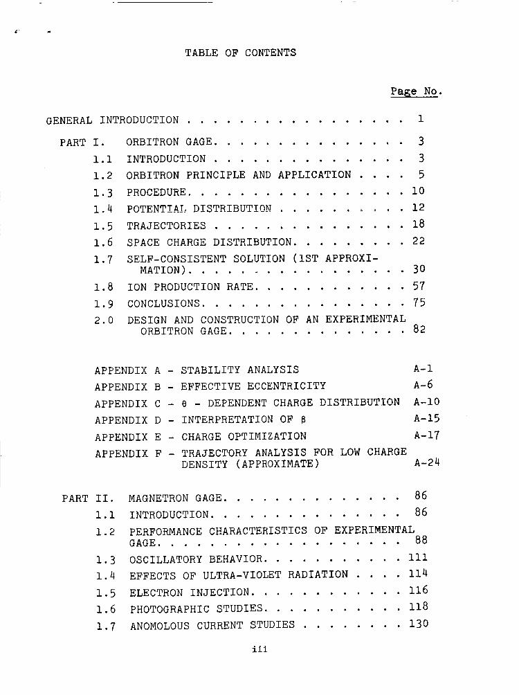
TABLE OF CONTENTS
Page No.
GENERAL INTRODUCTION .................
PART I. ORBITRON GAGE ...............
1.1 INTRODUCTION ...............
1.2 ORBITRON PRINCIPLE AND APPLICATION ....
1.3
1.4
1.5
1.6
1.7
1.8
1.9
2.0
3
3
5
PROCEDURE ................. l0
POTENTIAL DISTRIBUTION ......... 12
TRAJECTORIES ............... 18
SPACE CHARGE DISTRIBUTION ......... 22
SELF-CONSISTENT SOLUTION (IST APPROXI-
MATION) ................. 30
ION PRODUCTION RATE ............ 57
CONCLUSIONS ................ 75
DESIGN AND CONSTRUCTION OF AN EXPERIMENTALORBITRON GAGE .............. 82
APPENDIX A - STABILITY ANALYSIS A-I
APPENDIX B - EFFECTIVE ECCENTRICITY A-6
APPENDIX C - e - DEPENDENT CHARGE DISTRIBUTION A-10
APPENDIX D - INTERPRETATION OF 8 A-15
APPENDIX E - CHARGE OPTIMIZATION A-17
APPENDIX F - TRAJECTORY ANALYSIS FOR LOW CHARGE
DENSITY (APPROXIMATE) A-24
PART II.
i.i
1.2
MAGNETRON GAGE .............. 86
INTRODUCTION ............... 86
PERFORMANCE CHARACTERISTICS OF EXPERIMENTALGAGE ................... 88
1.3 OSCILLATORY BEHAVIOR ........... iii
1.4 EFFECTS OF ULTRA-VIOLET RADIATION .... 114
1.5 ELECTRON INJECTION ............ 116
1.6 PHOTOGRAPHIC STUDIES .......... 118
1.7 ANOMOLOUS CURRENT STUDIES ........ 130
iii

LIST OF FIGURES '
Page No.
FIG. 1
FIG. 2
FIG. 3
FIG. 4
FIG. 5
FIG. 6
FIG. 7
FIG. 8
FIG. 9
NUMERICAL SOLUTION OF EQ. (64) ........ 37
NUMERICAL SOLUTION OF_EQ. (68) FOR THE
MAXIMUM VALUE OF _ 2 = l) .......... 38
1ST APPROXIMATION TO THE SPACE CHARGE
DISTRIBUTION ................ 40
1ST INTEGRAL OF fl (mo'_ 41_eJ
2ND INTEGRAL OF fl (_o'_) ........... 42
2ND APPROXIMATION TO THE CHARGE DENSITYDISTRIBUTION ................ 45
EXPERIMENTAL ORBITRON GAGE (SCHEMATIC) .... 83
ELECTRON LAUNCHER (SCHEMATIC) ......... 84
MAGNETRON EXPERIMENTAL SETUP (SCHEMATIC) . . . 89
FIG. i0 EXPERIMENTAL MAGNETRON SCHEMATIC ....... 91
FIG. ll CALIBRATION CURVE 552 GAGE .......... 94
FIG. 12 EFFECT OF MAGNETIC FIELD AND ANODE VOLTAGE
ON MAGNETRON SENSITIVITY .......... 100
FIG. 13 EFFECT OF MAGNETIC FIELD AND ANODE VOLTAGEON MAGNETRON SENSITIVITY .......... 101
FIG. 14 MAGNETRON SENSITIVITIES VS. MAGNETIC FIELD . .102
FIG. 15 EFFECT OF MAGNETIC FIELD AND PRESSURE ONMAGNETRON SENSITIVITY ............ 105
FIG. 16 VALUES OF V A AND B AT WHICH NORMAL MAGNETRONIS LINEAR .................. 107
FIG. 17 NORMAL MAGNETRON CATHODE CURRENT VS. PRESSURE
(3000v, ll00 GAUSS) ............. 109
FIG. 18 EFFECT OF PRESSURE ON INTENSITY ON r-f
SIGNAL FROM MAGNETRON GAGE ......... ll2
FIG. 19 VIEW OF DISCHARGE THROUGH RADIAL SLOT INCATHODE OF MAGNETRON GAGE .......... 120
iv

LIST OF FIGURES
Page No.
FIG. 20 DISTRIBUTION OF PHOTO-RADIATION FROM
MAGNETRON GAGE .............. 121
FIG. 21 EFFECT OF ANODE VOLTAGE ON RADIAL DISTRI-
BUTION OF LIGHT .............. 125
FIG. 22 EFFECT OF MAGNETIC FIELD INTENSITY ON
RADIAL DISTRIBUTION OF LIGHT ....... 126
FIG. 23 POLARIZATION P AS A FUNCTION OF TIME
t AFTER A CONSTANT ELECTRIC FIELD IS
APPLIED TO THE DIELECTRIC ......... 135
FIG. 24 DIELECTRIC POLARIZATION EXPERIMENTAL TEST
ARRANGEMENT ................ 136
FIG. 25 CATHODE TO AUXILIARY CATHODE LEAKING CURRENT
VERSUS TIME AFTER A .170 VOLT STRESS WAS
REMOVED. (THIS STRESS WAS APPLIED FOR
32 MINUTES) ................ 138
FIG. 26 CATHODE TO AUXILIARY CATHODE LEAKAGE CURRENT
VERSUS TIME AFTER AN ANODE DISTURBANCE
(1 - HIGH VOLTAGE POWER SUPPLY TURNED OFF,2 - ANODE HEAD DISCONNECTED) ....... 139
V

v
LIST OF TABLES
Page No.
TABLE I
TABLE II
TABLE III
TABLE IV
TABLE V
TABLE VI
SENSITIVITIES OF MAGNETRON GAGE AT AN
AVERAGE PRESSURE OF 5.2 x l0 -8
(TORR N 2 ) ................ 96
SENSITIVITIES OF MAGNETRON GAGE AT ANAVERAGE PRESSURE OF 5.2 x 10⁻¹⁰ TORR. . • 97
SENSITIVITIES OF MAGNETRON GAGE AT AN
AVERAGE PRESSURE OF 2.7 x i0 -II TORR. . . 98
SENSITIVITIES OF MAGNETRON GAUGE AT AN
AVERAGE PRESSURE OF 1.2 x 10⁻¹¹ TORR. . . 99
EFFECT OF ANODE VOLTAGE (V A) VARIATIONSON INTENSITY OF DISCHARGE IN ARGON .... 123
EFFECT OF MAGNETIC FIELD VARIATIONS (B)
ON INTENSITY OF DISCHARGE ON ARGON ..... 124
vi

@.
SUMMARY
During recent years it has become increasingly apparent
that the techniques for the production of an extremely low
pressure environment have outstripped the methods and tech-
nigues of measurement of low pressure. The present work
represents part of a continuing effort to develop more reliable
and higher sensitivity pressure gauges for pressures below
l0 -10 Tort. The report is divided into two parts. Part I is
a consideration of the orbitron gauge. This type of gauge
appears to have high potential for the measurement of extremely
low pressures. In addition it appears to have high potential
for aerospace pressure measurements because it does not require
magnets of relatively high mass.
The major fraction of the present work on the orbitron
is concerned with a theoretical analysis of the orbitron prin-
ciple. In this part of the program a method has been developed
for obtaining a self-consistent solution for the electron motion,
charge density distribution, and space charge dependent potential
distribution in an orbitron. The solution may have any pre-
scribed accuracy, since the final accuracy of the solution is
a function only of the number of iterations performed. The
assumptions used are equivalent to asserting that the space
charge is all electronic and is only a function of r (these
are later shown to be valid for practicable configurations
and modes of operation). The interelectrode space is divided
into 3 concentric cylindrical regions such that all the space
charge is contained in the middle region. The Poisson Equation
is solved in the middle region for an arbitrary charge distri-
bution and matched at its boundaries with solutions of the
Laplace Equation in the adjacent regions. The force equations
are solved for the radial component of the electron velocity
for an arbitrary potential distribution. The continuity equation
is solved for the charge distribution for an arbitrary electron
vii

radial velocity. The ist approximation to the charge distri-
bution is obtained by using the space charge free electron
radial velocity. This charge distribution is substituted into
the potential distribution and integrated numerically to giventhe first approximation to the space charge dependent distri-
bution. This result is substituted into the radial velocity
equation to obtain the 2nd approximation to the electron radial
velocity which is substituted back into the continuity equation
to obtain the 2nd approximation to the charge distribution andbegin the 2nd iteration. A comparison of the 1st and 2nd
approximations of the charge distribution indicates that the
iteration process converges rapidly and that the result of
the 1st iteration is a useful approximation to the self-consistent solution.
The Ist iteration has been worked out for a particular
subset of self-consistent solutions. Using these results as
a 1st approximation to the final self-consistent solution,
conditions are derived which optimize the total space chargestored in the rotating electron cloud such that the electron
trajectories are stable and the space charge distribution is
uniform in e-space and the electron mean kinetic energy has
a prescribed value. Under these conditions, it turns out
that the total space charge stored in the rotating electron
cloud approximates that stored on one plate of a cylindrical
capacitor which has the same dimensions and anode potential.
It is found that the ion current generated per centimeter of
length of the lectron cloud (along the z-axis) is of the
order of 1 to 15 amp/Torr (Argon) for anode potentials in
the range 0.4 to 10KV_ This corresponds to ionic pumping speeds(for Argon) of the order of 0.2 to 3 liters/sec (for each
centimeter of pump length) and to ion gage sensitivities ofthe order of l0 4 to l0 5 Torr -1 (Argon) for a conventional
size device (l=10 cm). Further it is found, in ion gage
viii

applications, that modes of operation are possible which are
substantially free of x-ray induced residual current.
An experimental orbitron gage for extremely low pressure
measurement was designed and constructed but performance
characteristics were not measured during the present program.
Part II of the present report outlines work carried out
on the normal magnetron type of gage. The major emphasis
of this part of the program was on the measurement of the
senslvities of a normal magnetron gage over wide ranges of
anode voltages, magnetron field strengths and pressures.
Sensitivities were measured at the following pressures:
5.2 x l0 -8 Torr, 5.2 x l0 -10 Tort, 2.7 x l0 -ll Tort, and
1.2 x l0 -ll Torr. Anode voltages were varied from 1000 to
8000 volts and magnetic field strengths from ll00 to 2000
gauss. The study confirmed earlier work and showed that
considerable changes in gage sensitivity may occur as the
operating parameters are varied. However, broad general
patterns exist in the performance characteristics and gage
sensitivities may be more than doubled from the 4.5 amp/Torr
obtained at about 5000 volts and i000 gauss if considerably
higher anode voltages and magnetic field strengths are used.
Some evidence was developed which suggested that the linear
operation of the normal magnetron could be extended to lower
pressures by operating the gage at different combinations of
anode voltage and magnetic field strength -- e.g., 3000 volts
and ii00 gauss, also 4800 volts and 1250 gauss. However,
it appeared that a lower pressure limit was obtained for the
range where the gauge was linear or close to linear for these
conditions also. For instance, with an anode voltage of 4800
volts and a filled strength of 1250 gauss the gage had a
response curve with a slope of approximately 0.9 down to
1.2 x i0 -II Tort. But the results indicated that the gage
again turns to non-llnear operation at lower pressures.
ix
A short study was made of the r.f. oscillatory behavior
of the normal magnetron gage. The results obtained confirmed
previous measurements. The generation of stable r.f. frequencies
could not be detected below 2 x I0 -I0 Torr-the pressure below
which the gage is non-linear.
Experimental work on the effects of ultra-violet radiation
and electron injection were inconclusive because of possible
effects of photo-desorption and thermal desorption.
Work was initiated on the theoretical and practical
aspects of some of the possible sources of anomolous currents
at the cathode of the magnetron gage.
A large number of photographs of the discharge inside
the experimental magnetron gage were taken. From these it
was possible to estimate the shape of the discharge and its
intensity. The effects of pressure, anode voltage and
magnetic field strength on the discharge were broadly examined.
It was not possible to obtain photographs of the discharge
below 2 x i0 -I0 Torr.
GENERALINTRODUCTION
As a part of a previous program (NASw-625), the operating
characteristics of four UHV ionization gages were examined atpressures below l0 -10 Tort. The gages chosen for study were
those which appeared to have the highest potential for the
measurement of extremely low pressures. They were a nude
modulated Nottingham gage, a suppressor-grld gage, an in-
verted magnetron gage, and a normal magnetron gage. The
work indicated that the normal magnetron gage should continue
to be included in the further investigations of the measurement
of extremely low pressure mainly because of its high sen-
sitivity and the fact that hot filaments were not required
to supply the ionizing electron flux. The work clearly in-
dicated that a considerable improvement would result if the
linear region of the normal magnetron gage were extendedbelow 2 x l0 -10 Tort. It therefore became the aim of the
present program to investigate the possibilities of "llnearizlng"
the normal magnetron and to improve its low pressure operating
characteristics. One of the aspects considered under the
latter heading was the possibility of reducing the noise
level of the gage at low pressures. This was to include
the reduction of spurious currents arising from mlcrophonlcs,
dielectric polarization, and leakage.
In addition, it had become apparent in the period of
performance of the first program that another gage, not
investigated in that program also held considerable promisefor low pressure measurement. This was the orbitron gage_1)"
Consequently, theoretical and experimental investigations
of the orbitron gage were initially included in the present
program.
The work carried out under the present program is divided
up into two parts. Part I is a report of work carried out
in the present program on the orbitron gage. The major fraction

is connected with a theoretical analysis of the orbitron
principle. The second section of Part I describes work onthe design and construction of an experimental orbltron
gage. This work predated the theoretical analysis and inconsequence it was not feasible to incorporate the resultsof the theoretical analysis in the design of the experimental
orbitron gage. Part II is a report of the various aspects
of work carried out on the normal magnetron gage.

Part ! ORBITRON GAGE
I. i INTRODUCTION
The orbitron principle has been applied to ion gages and ion pumps
by the group at the University of Wisconsin under the direction of
Professor R.G. Herb. (I)The activity of this group has been principally
applied to the experimental development of practical pumps and gages
with a secondary emphasis on the theory and analysis of the orbitron prin-
ciple. The theory of the orbitr0n principle appears to have been studied
first by W.E. Waters (2) and then independently by R.H. Hoover_nan, (3)
stimulated by Herb's work. However, in both of these studies only the
space charge free potential distribution was considered. While the re-
sults of these studies may correctly describe the electron trajectories
for a very low electron density stored in the rotating electron cloud, the
results are not applicable to practical orbitrons since existing experi-
mental data indicate that the electron density in the space charge cloud
is not negligible, in fact it may even approach saturation. The space
charge free analysis yields little, if any, insight into the dynamics of
the orbitron since all the questions of subst_ice involve the space charge
dependent potential distribution. For example, questions concerning
electrode geometry for optimum charge storage in the rotating space charge
cloud, launcher location for optimum charge storage, anode potential for
optimum charge storage, self-consistent orbit injection parameters, mean
orbiting life-time of the electrons, orbit stability criteria, dependence
of average kinetic energy of the electron on stored charge, and injec-
tion (emission) current necessary to maintain optimum charge storage can
not be answered without knowledge of the space charge dependent potential
distribution.
The orbitron principle appears to contain a natural feedback mech-
anism which, for a given electrode geometry and potential, and a self-
consistent set of prescribed injection parameters, launcher location and
injection current, limits the number of electrons stored in the space
charge cloud. However, it appears possible to over-ride this feedback
mechanism and over-populate the electron cloud if all geometrical, elec-
trical and dynamic parameters are not self-consistent. The over-popula-
tion of the electron cloud substantially modifies the potential distribution

such that the injection parameters now violate the orbit stability criteriaand the electron meanlife-time is reduced to transit time between the
launcher and anode.
Fromthe above discussion it is clearly essential that the analysis
of the orbitron be self-consistent if it is to be applicable to real orbl-t-
rons, provide insight into the principle, and provide answers to the prac-
tical questions implied above. That is, the analysis must be self-consistent in the sense that the differential equations which describe the
electron motion must contain a potential distribution which is in part a
function of the electron motion and thus take proper account of the aver-
age electron distribution within the space charge cloud. This appears to
be a formidable task, since the self-consistent set of differential equa-tions describing the electron motion (Force Equations, Poisson Equation ,
and Continuity Equation) reduce to an essentially nonlinear integral
equation of a type for which no general solution is known (except, perhaps,
in a few special, restricted cases). However, a solution to the self-
consistent set of equations is possible using iterative, numerical methods.
A method of solving these equations such that the solution has a pre-
scribed accuracy is outlined later on and the first approximation is
worked out in somedetail. Even from this approximate solution, consider-
able insight into the answers to manyof the above questions is developed.

J_
I. 2 ORBITRON PRINCIPLE AND APPLICATION
In principle, the orbitron consists of two coaxial cylinders having
radii R. (inner) and R (outer), between which is applied a potentiali o
difference V(Ri)_0 and V(Ro)=0 , yielding a logaritb_ic electrostatic
potential distribution in the interelectrode space and a central force
field which is attractive for electrons. It is assumed that the cylinder
lengths are large con_pared to their radii thus minimizing the importance
of end effects. Electrons are injected into the central force field with
angular momentum and kinetic energy such that they are captured in bound,
stable orbits around the inner cylinder (anode). For certain sets of
orbit injection parameters the individual electron trajectories resemble
open ellipses as viewed from a stationary reference system. While the elec-
trons execute ellipse-like trajectories in a radial plane they drift slowly
in the axial direction until they arrive in the neighborhood of the end of
the coaxial cylinders, where they are reflected by a weak electron mirror
field (produced by auxiliary electrodes). Thus the total trajectory is
s_milar to an elliptical spiral repeatedly folded back on itself.
If the individual electron orbits are not closed, the electrons col-
lectively form a space charge cloud, the charge density of which is
uniform in azimuth and the local angular velocity of which is equal to
the average angular velocity of the electrons at that radius. Thus, not
all parts of the cloud have the same angular velocity; the inner part of
the space charge cloud rotates at a much higher angular velocity than the
outer part of the cloud.
Although, under the proper conditions, the charge density of the space
charge cloud is uniform in 0-space, it is never uniform in r-space. The
electron cloud does not occupy the entire interelectrode space but rather
has an inner and outer boundary which corresponded respectively to the
inner and outer turning points in the electron trajectories. The radial
charge density is proportional to the interval of time that the electron
occupies an increment of the radius between the inner and outer turning
points (inner and outer cloud boundaries). Thus the radial charge den-
sity distribution is inversely proportional to the radial component of

the electron velocity. The charge density is thus high in the neighbor-
hood of the boundaries and low in the neighborhood of the radial center
of the space charge cloud.
The electronic (negative) space charge associated with the rotatingelectron cloud modifies the interelectrode electrostatic potential dis-
tribution. The potential distribution associated with the electron den-
sity distribution is always negative, regardless of the particular shapeof the density distribution. Thus the total potential distribution, that
due to applied potential plus that due to interelectrode electronic space
charge, is everywhere lower than the applied potential distribution.Therefore the electric field inside the inner space charge boundary is
higher than the applied electric field and the field outside the outercloud boundary is lower than the applied electric field. Thus, within
the cloud the field gradient (total) is much steeper than it would be if
the space charge density were negligibly low. Thesemodifications of the
potential and field distributions obviously have strong effects on themotion of the electrons which produced them. This is the source of nearly
all the difficulties in understanding and in applying the orbitron prin-
ciple. For very low space charge densities where the actual potentialdistribution is nearly identical with the applied potential distribution
the orbitron principle is simultaneously elegant and simple, and is almostcompletely understood. (1'2'3) Howeverthe principal advantage of real
orbitrons is the ability to attain relatively high charge densities.
The value of applying the orbitron principle to ion gages and ion
pumps is that large numbersof electrons having long mean life-times may
be stored in the space charge cloud and efficiently used to generate ions
by impact ionization. This, of course, assumesthat the electrons are
injected into stable (long life-time) trajectories, a condition which re-
quires a knowledge of the space charge dependent potential distribution.
There is another substantial advantage in applying the orbitron principle
to ion gages: It appears possible to operate an orbitron ion gage in a
modewhich produces no soft x-ray induced background current. In conven-
tional ion gages, electrons having kinetic energy in the neighborhood of

i00 eV are abruptly decelerated in the surface of the electron
collector (grid). A fraction of the soft x-rays produced by thedecelerated electron flux are radiated from the electron collec-
tor surface to the ion collector surface, and produce free elec-trons by the phoeoelectric process. (The electrons which
have final momentum vectors such that they penetrate the surface
barrier and escape into the vacuum.) The photoelectric current
leaving the ion collector is indistinguishable from an ion cur-
rent arriving at the collector. Thus there exists a background
or residual current which is dependent only on the emission cur-
rent. In the orbitron, provided the electrons are properly in-
jected into stable orbits, the electrons do not reach the anode
except if they have lost sufficient energy in a collision to make
it energetically possible. A large fraction of the collisions of
this kind are ionizing collisions (for electron energies in the
neighborhood of i00 eV). Thus the subsequent emission of a photo-
electron at the ion collector (outer cylinder), by a soft x-ray
emitted from the anode in the process of collecting the ionizing
electron, simply enhances the current associated with the ionizingevent. Those electrons which do not encounter a gas atom continue
to orbit the anode until they eventually return to the launcher,or exit from the orbitron structure. It appears possible to
arrange the potential of the launcher such that returning elec-trons arrive with a relatively low kinetic energy, under which
condition the generation of soft x-rays is an improbable process.
Thus, operation of an orbitron ion gage in this mode avoids the
usual defect of generating a residual current which is dependent
only on the emission current.
The relization of the advantages inherent in the orbitron
principle, in applications to practical ion gages and ion pumps,
requires optimization of the total ionization rate. The prin-
cipal parameters involved in this optimization are: orbit stabil-
ity,the electron kinetic energy, space charge cloud location,
7
and the number of electrons stored in the space charge cloud
(per unit length). There is considerable value in a brief, pre-liminary observation of how these parameters influence the
application of the orbitron principle to a practical device.
The probability of an electron encountering a gas ato_of course, in-
creases as the electron orbiting life-time increases. The probable orbit-ing life-time is maximumfor stable orbits. Thus the electrons must be
injected into stable orbits.
The probability that an electron-atom collision yields an ion (in an
inelastic collision) is a functioh of the kinetic energy of the electron.
The maximumionization probability in most gases occurs for an electron
kinetic energy in the neighborhood of I00 eV. However, the ionization
probability as a function of energy generally falls off much faster for
energies less than this value than it does for energies greater than this
value. Thus the electrons must be injected into orbit such that their
minimumkinetic energy (outer turning point) is not substantially less
than the kinetic energy corresponding to the ionization efficiency maxi-
mum,eventhough the kinetic energy is substantially above this value at
the inner turning point.
The ionization rate (per unit length), of course increases as the num-
ber of orbiting electrons in unit length of the space charge cloud in-creases. The maximumnumberof electrons that can be stored in unit
length of the cloud is a function of the electron kinetic energy, the orbit
stability, the applied potential, and all geometrical parameters. The
requirements of the above two paragraphs, in effect, specify the first
two of these parameters and also assign a minimumvalue to the applied
potential. Thus the geometrical parameters and the maximumvalue of theapplied potential must be chosen such that the number of electrons in unit
length of the cloud is maximized.
Failure to follow the above pre scriptions, in one way or another reduces
the ionization rate below its optimum value (although the stored charge
may actually increase) and increases the residual current (in ion gage ap-
plications). The details of the methods of satisfying the above require-

ments are developed later on.
There are several important constraints which should be
recognized in any application of the orbltron principle topractical devices. The ratio Ro should not be too large.
Ultimately, the quantity of charge that may be stored in the
electron cloud depends on the field-energy density within theinterelectrode volume. As R° increases the total field-
Roenergy decreases. Further,--for _i large, the field-energydensity is high only in the neighborhood of the anode and
low elsewhere. Thus as _ increases the useful fractionof the volume within thea_nterelectrode space shrinks. ForRoR_i large, a non-negligible fraction of the total populationof the electron cloud may be electrons that have already
experienced one or more collisions with gas atoms, since the
probability of capturing an electron at the anode immediatelyR° increases.
following a collision decreases asThe electron trajectories should be such that regions of
low electric field are avoided since in these regions the
magnetic forces on the electron (arising from spurious magnetic
fields) may be comparable with the electric forces.
9

1.3 PROCEDURE
It is considered useful to outline here the analytical
procedure that is followed in subsequent sections since some of
the analyses are rather long, some intricate, and some encounterrather cumbersome analytical expressions. To minimize the pos-
sibility of arithmetic inundation some of the demonstrations and
computations have been placed in appendices.
The first step in the procedure consists of solving Pois-
son's Equation for an arbitrary charge density distribution ex-
tending over an arbitrary region of the interelectrode space.
It is therefore necessary to divide the interelectrode spaceinto three concentric regions and solve the Poisson Equation in
each. The solution for each region is then matched at its
boundaries with the solutions for the adjacent regions. In the
process, electrode boundary conditions are applied. Three ex-
pressions are finally obtained for the potential distribution,
one for each of the three regions, in terms of the applied po-
tential, geometrical parameters and integrals over the arbitrary
charge density distribution.
The differential equations (force equations) for the mo-tion of an electron are solved for an arbitrary potential dis-
tribution. Only a solution for the velocity is required since
the turning points may be obtained directly from the velocity
equation and a detailed knowledge of the orbit shape is unneces-
sary in nearly all meaningful questions. However, much can be
inferred concerning the general orbit shape from various
analytical results. In developing an expression for the veloc-
ity it is useful to distinguish between stable and unstable
trajectories. The results of the stability analysis are in-
corporated into the velocity equation.
I0
The charge density distribution is then obtained from
the continuity equation in terms of the radial component of
the electron velocity. The same expression is derived fromstatistical reasoning.
At this point three equations have been obtained in
terms of three unknown functions: the potential distribution,
the charge density distribution, and the electron velocity.Solving this system of equations for the potential distribu-
tion yields a nonlinear integral equation. This equation has
a form for which no general solution is known. However, a
particular solution is possible using numerical techniques.
By numerical integration and iteration, a solution having anyprescribed accuracy may be obtained.
The electron velocity corresponding to the space chargefree potential distribution is taken as a first trial solution.
The space charge free electron velocity is integrated numeric-
ally and the result used to obtain a first approximation to the
space charge dependent potential distribution. Inserting thispotential into the electron velocity equation yields a second
approximation for the charge density distribution.
This procedure, although not done here, may be continued
until a solution is obtained having the prescribed accuracy.
The additional computation required to obtain a convergent,self-consistent solution involves considerable computer time.
11

1.4 POTENTIAL DISTRIBUTION
In solving Poisson's Equation for the space charge depend-
ent potential distribution, it is unnecessary to consider all
possible charge density distributions. Rather, only those dis-
tributions are considered which lead to near optimum electronstorage, since the principal function of the electron cloud is
to generate ions, which can be done at the maximum rate if the
number of electrons stored in the cloud is optimized. It is
obvious that those charge density distributions which are most
uniform in 0-space, produce the smallest modification of the
electrostatic potential distribution for a prescribed total
charge. Since the electron orbits must remain stable and the
electrons must have a kinetic energy greater than a prescribed
minimum, there is a limit to the magnitude of the space chargemodification of the electrostatic potential distribution thatcan be allowed.
A uniform charge density distribution in the radial direc-
tion is incompatible with the differential equations which de-
scribe the motion of orbiting electrons. Thus the applicable
form of Poisson's Equation will always have at least one inde-pendent variable, r.
If the electron drift velocity in the z-direction is suchthat the period of oscillation in the z-direction is a non-
integral multiple of the orbit period, the charge density dis-
tribution is nearly uniform in the z-direction, except in the
neighborhood of the electron mirrors at the ends of the cylin-
ders where the charge density increases slightly since the
mirrors introduce z-direction turning points. It therefore is
allowed to eliminate z as one of the independent variables in
Poisson's Equation, a considerable simplification. Formally
stated then, the first assumption in the analysis is: The charge
density distribution is sufficiently uniform in the z-direction
that its variation may be neglected in the analysis.
12
Concerning the dependence of the charge density distribu-
tion on e, the situation is not so elementary. Both uniform
and strongly e-dependent charge distributions are possible.
This may be seen more clearly by considering first, those trajec-tories which lead to e-dependent charge density distributions.
If electrons are injected into trajectories which close after
the execution of n orbits, the complete trajectory of the
electrons resembles n superimposed, open-ellipse-like trajec-
tories such that the angle between successive outer turning
2m_ (See Appendix C). The electron continues inpoints is n "this trajectory indefinitely, retracing it once for each mcircuits around the anode. That is, for a closed trajectory
the electron returns again to the point of orbit injection,
same r and 0 but different z, and passes through this
point with the same kinetic energy and angular momentum that itpossessed at orbit injection. It necessarily follows that
trajectories of this type are stationary since the individualorbits of the anode resemble ellipses having a relatively large
counter rotating precession velocity such that the major axisrotates about the anode exactly m times while the electron is
orbiting the anode n times. If all electrons are launched
from the same point and injected into orbit with the same angu-lar momentum and kinetic energy (which is very probable), then
all electrons proceed along the same closed trajectory. Thus
the charge density distribution in 0-space is nonuniform, being
concentrated principally in the neighborhood of the 2n turning
points of the n superimposed ellipse-like trajectories, and isstationary. Even if the electrons were all injected at equal
intervals in time, at any given instant later they are not equally
spaced along their common trajectory. These motions are investi-
gated quantitatively in Appendix C.
It is clear, by comparison with the above results, that
open trajectories lead to charge density distributions which areuniform in 0-space. That is the result of the continuing pre-
cession of the orbit eventually smears the charge uniformly
13

through e-space. This conclusion holds even if all electrons are
injected into the same open trajectory. As stated previously,
optimum charge storage is associated with the absence of chargeclusters, that is with uniform charge density distributions.
Thus the second assumption, implicit in the following analysis
is: The charge distribution in e-space is uniform, that is that
the range of allowed orbit injection parameters are such that the
electron trajectories are open or at least close only after n is
very large. This eliminates e as an independent variable in
Poisson's Equation and reduces it and the continuity equation to
one dimensional ordinary differential equations in r.
Since the electron trajectories do not occupy the entire
interelectrode space but rather only a thick cylindrical region
located somewhere within the interelectrode space and with its
axis coinciding with the axis of symmetry, it is necessary to
divide the interelectrode space into three thick cylindrical re-gions: Region i e the volume between the anode surface and the
inner boundary of the electron cloud; Region 2 e the volume
occupied by the electron cloud; Region 3 e the volume between the
outer boundary of the electron cloud and the surface of the outer
cylinder. A radial cut through the interelectrode space is shown
in the figure below, which also defines some of the pertinentparameters V-
¢(r) ¢i (r)/ I(r)
ri0 _- ;--r
Ri I I R °
Ii 0(r)I
In Region I, the potential distribution ¢i(r) is obtained
from the homogeneous Poisson Equation (Laplace Eq.)
i d _ d¢1_ = 0 (R i_r<__ri). (I)r dr t (--d-_
14

In Region 2, the Poisson Equation applies
i d ir d¢2 (r)Yd--r _-'-) - P0
, (ri__ r __ ro).
In Region 3, the Laplace Equation again applies
(2)
i d [r d¢3r dr _---) = 0 , (ro_r_Ro). (3)
At the boundary between Reg_on_ I &rid 2, the .... _.... _t_,_ distribution and
the electric fleld must be continuous. Therefore the solutions to
Eqs.(1) and (2) must satisfy
¢l(rl) : ¢£(rI) ,(4)
and
de 1 = de
1 I
(5)
At the boundary between Regions 2 and 3 again the potential and electric
field must be continuous. Therefore the solutions to Eqs.(2) and (3) must
satisfy
@2(to) = ¢3(r0>,(6)
and
d¢2 de 3
dr r=ro r:ro
(7)
At the surface of the anode, the potential must equal the applied voltage
V. Therefore
¢l(Ri) = V .(8)
15

At the surface of the outer cylinder the potential must be zero.
fore
¢3(Ro) : 0
There-
(9)
The solutions to Eqs.(1), (2) and (3) are (before evaluating the
constants of integration)
el(r) : Cll log r + c12 , (R i _< r _< ri) ,
¢2(r) =_ f dr (r) r dr + c21 22 , - --_- f P log r + c (r i <r<ro) ,C o
¢3(r) = C31 log r + c32 , (r o _< r_< Ro).
(i0)
(ll)
(12)
Using the six conditions expressed in Eqs.(4) through (9) to evaluate
the six constants of integration gives
Ro R R° log rv O
(r) = V l°g-_--r-+ {l(ro)-l(ri) +I (ro)l°g _--- l'(ri)l°g r7 } _ii_1 log Ro o 1 log _R° '
RRi ±
(R_ _ r _ ri),(13)
_2(r) = V
R log r
log -_0 E1 R°]
r + (ro)+l' (ro)log _--log __R° o log
R.i
R
[I rg<._ l°g °+ (ri)-l'(ri)lo -r- l(r), (ri -<r _<ro),• log Ro
R.1
¢3(r) --V
RO
log r
log RoR.
1
(14)
R
r ri I l°g--q°o I' )log r(r°)-l(ri)-l'(r°)l°g_ii + (ri Vii log __R°'
R.i
(ro _ r _ Ro), (15)
16

where
l'(r x) = f p(r) r drJ_0 r--r X
(16)
and
dr (r)l(rx) = f _- f _eo
rdrIr=r
x
(17)
Equations (13) through (15) define the interelectrode potential distribu-
tion in terms of geometry, applied potential, and the charge integrals in
Eqs.(16) and (17) for an arbitrary charge distribution, the evaluation of
which must await specification of the actual charge density distribution
from the results of the orbit analysis.
17

i. 5 TRAIECrORIES
The differential equations for the motion of an electron in a cylindri-cally syn_etric attractive, central force field are:
and
m (_ - re 2) = -eE(r), (radial force component),
d_(mr26) = 0, (azimuthal component),
(18)
(19)
where E(r) _ electric field due to both the applied potential
and the space charge distribution.
IntegratingEq.(19) gives
= (20)
where
z electron angular momentum (a constant throughout the
orbital motion).
Therefore Z is one of the orbit injection parameters. Using Eq.(20) to
eliminate e in Eq.(18) gives the radial force as a function of r alone
m_'- &2 eE(r). (21)mr 3
The space charge radial distribution must eventually be derived from the
solution to this equation.
Before proceeding with the solution of this equation, it will be
rewritten to satisfy the orbit stability criteria, that is it must be
modified such that it applies only to stable electron trajectories and
excludes from consideration all trajectories which are unstable against
radial perturbations. The motivation for introducing this modification
is simply to concentrate the analytical work on that subset of trajec-
tories which has the longest probable orbiting life time, since in
18

practical devices these trajectories are the most useful. There are
many disturbances which may perturb the electron trajectory; for ex-
ample, variation in electrode potentials due to power supply noise,
variation in potential distribution induced by collective space charge
oscillations, local magnetic fields, motion of the orbitron in these
fields, elastic (nonionizing) collisions with gas atoms, etc. It is ob-
vious that those trajectories which areunaffected by such disturbances
have the highest probability of survival. Those trajectories which are
least affected are the stable trajectories.
It is shown in Appendix A that the open-ellipse-like trajectories are
stable only if the electron angular momentum satisfies the stability cri-
teria
£2 = m2meE (ro)ro3 (22)2
where e is an independent stability parameter which quantitatively labels
th_ stability of an _t _nd has the allowed _'ange
1 m2(approaching instability) _ < & 1 (most stable) . (23)
* _ the effec-It is shown in Appendix B that e is a function only of ec
tire eccentricity of the open-ellipse-like electron trajectories in the
orbitron. It is shown in Appendix C that there are certain discreet
values of e within the range given by Eq.(23), but which must be dis-
allowed since they not only violate one of the analytical assumptions,
but lead to stationary nonuniform charge distributions in 0-space and
therefore nonoptimum charge density distribution.
Thus, the modification which must be made in the radial force equa-
tion, Eq.(21), is simply to introduce the stability criteria into that
equation such that the system of equations applies to stable orbits only.
Essentially, this constrains the allowed range of one of the orbit in-
Jection parameters (angular momentum) to a relatively narrow range.
19

I
The actual constraint, which sorts out of all possible electron
trajectories those which are stable, is introduced into the system by re-
placing the angular momentum in Eq. (21) with its constrained value given
by Eq. (22). The radial acceleration of the electron, applicable to stable
orbits only, then is given by
e [a2E2(ro ) ro 3 E (r)]r'=m rT- 2 "
(24)
This introduces a third formal assumption into the analysis: Allowed
orbits are members of the orbit subset which satisfy the stability criteria
Eq. (22) only, however there is a discreet series of orbits within this sub-
set which are disallowed since they lead to stationary nonuniform charge
distributions in e-space.
Proceeding now with the solution to Eq. (24), the radial component of
the electron velocity is obtained by multiplying this equation by dr,
recalling that "r_ir= _ , that -E(r)dr = d[¢(r)], and integrating.
The result is
_.,2 = __2e_-e2ro3E2(ro)____ +¢2(r)I + c , (25)m L 2r 2
where c is a constant of integration. This constant may be conveniently
evaluated at either the inner or outer turning points where the radial
con_ponent of the electron velocity passes through the value zero. There
is, however, some advantage in using the outer turning point. Thus,
setting the left side of Eq.(25) equal to zero, evaluating the right side
at r=r o, solving for c, and substituting the result back into Eq.(25)
gives the radial velocity in terms of physical parameters
_2 2eFs2roE2 (r°) (i ro 2 )_= -m-L 2 " - r-_- ] + @2(r)-¢2(r° "(26)
2O
This equation has two roots: the larger is of course at ro, the
smaller is at ri (the inner turning point) which may be obtained by
setting r2=0 giving the transcendental equation
2 { (ri) _ _2(ro) }
ro 2 _2
ri 2=I + ....C_2 E2(ro)r ° •
(27)
The potential distribution in Eq.(26) is that previously obtained
for the space charge region, Eq.(14_. The electric field at the outer
turning point is obtained from Eq.(14) by taking the negative derivative
with respect to r and evaluating the result at ro. Both of these
functions depend, in part, on the charge density distribution through the
charge integrals, Eqs.(16) and (17), which are yet unspecified. Further
progress in developing a self-consistent solution for the electron motion
in the orbitron requires the definition of the charge density distribu-
tions.
21

1.6 SPACECHARGEDISTRIBUTION
Recalling the previous discussion concerning the possible form of
the charge density distribution, it was concluded that it could not be
a function of z since only small gradients existed in the Z-direction
resulting in a charge density which is nearly uniform in the Z-direction,
and that it could not be a function of e since only those launch param-eters corresponding to open orbits (nonstationary) are allowed, which
after sufficient time result in a charge density distribution which isuniform in the e-direction. If sufficient time is allowed after the be-
ginning of injection,the charge density at all points in the electron
cloud will have built up to its final, equilibrium value and will thus be
independent of time. This neglects the small time dependent componentof
the charge density associated with the collision loss rate and the orbit
injection rate, since the meanorbiting life-time is relatively long
(except at high pressures) in comparison with the injection or loss
transit time. This amounts to introducing into the analysis a 4th _or_nal
assumption: The time-dependent componentof the charge density distribu-tion corresponding to the collision loss rate and the balancing injection
rate is negligible in comparison to the stationary (equilibrium) charge
density distribution.
Under the above conditions the charge density distribution is a
function of r only, and thus the continuity equation
reduces to
v.j + -0_t
d(r_jr) = 0.dr
(28)
(29)
22
For any equilibrium (stationary) charge density distribution _P -• y_-o.
It necessarily follows that the quantity of charge flowing into any volume
element equals the quantity flowing out of that element. The radial compon-
ent of the current density at any point within the space charge region must
therefore consist of a positive and negative component, such that
and
ijr+(r) = _ o (r)_+(r) (30)
iJr_(r) = __ 0 (r)__(r) (31)
and have the property
• iJr(r) = Jr+(r) + jr_(r) = _p(r)[#+(r)+__(r)] = 0, (32)
since
#+(r) = -__(r) ; (33)
since b(r) is a single valued function of r. However, since all the.
charge is electronic and p (r) is a scalar, the charge density is inde-
(r). Thus each component of Jr(r) con-pendent of the sign of Jr
tributes equally to the local charge density 0(r). Therefore the function
that must be inserted into Eq.(29) for the current density is
•
IJr+(r) l + IJr-(r)] = 7 p(r)[ Ir+(r)[+ Ib_(r)l] = p (r)I_(r)
The contunuity equation thus becomes
(34)
d {r o(r) l_(r)l}= o.dr
The solution to this equation is obviously
(35)
p(r) -r]_(r) l
(36)
23

The constant of integration may be evaluated as follows: Supposethere
are NL electrons in unit length of the electron cloud (unit lengthalong the cylindrical axis). The integral of the charge density dis-
tribution over the volume of a uni t length of the space charge region
must equal the total charge within that region, thus
0(r) rdrd0 ---eNL
r. o1
(37)
where (-e)_electron charge.
equation may be written
Substituting from Eq.(36) for
Since 0(r) is independent of e this
ro
f eN Lp(r)rdr -27
ri
0(r) and solving for the normalization
constant c, gives
(38)
eNL iC -
27 l-1 ri
Substituting this result back into Eq.(36) gives the charge density dis-
tributionwithin the space charge region
(39)
0(r) = -
eNL i
• -m
f l (r) l-'dr rl (r) lr.
1
(40)
Although this result (that the charge density is inversly proportional
to the radial component of the velocity) is not a con_non form of charge
density distribution, it has been encountered in other situations (see for
exan_ole Landau and Lifschitz in Ref.5 where a similar result is obtained
in another connection concerning the motion of bound electrons).
24

The charge density distribution maybe derived directly from
statistical considerations which do not involve (explicitly) the inte-
gration of the continuity equation. This derivation also yields a some-
what different insight into the connection between charge density dis-
tribution and the electron dynamics. Consider the motion of a single
electron along a stable trajectory in an orbitron. The fraction of the
orbit period that the electron spends in traversing the infinitesimal
interval As along its trajectory s is
t(s÷As) - t(s) (41)
where • is the orbit period and t is considered a function of orbit
position s. The probability that the electron is within the interval
As at s is the probability distribution ¢ (s) (probability per unit
length of trajectory). Thus ¢(s) is simply the fraction of the orbit
period spent in as divided by the length of as,
¢(s) :t(s+as.)- t(s)
_ As(42)
Taking the limit A s÷ 0 gives
1 (43)- iv(S)l ,
since
lim t(s÷As)-t(s) _ dt ias+O As - ds : v_7 (44)
where _ s) e orbit velocity as a function of the trajectory coordinate s,
and the absolute value of the orbit velocity has been taken to avoid the
possibility of a physically meaningless negative probability distribution
(especially later, when a transformation is made from the trajectory co-
ordinate s to polar coordinates r,O). The charge associated with a single
electron may be considered as distributed over the electron orbit in exactly
the same way that the probable position is distributed. The charge dis-
tribution at any point s along the orbit is then given by the product of
25

the electron charge and the position probability distribution. Thus the
increment of charge in the interval ds at s is given by
dQ(s) = -e ¢(s) ds
Referring to the figure below, the increment of charge contained in the
volume between two concentric cylindrical surfaces of radii r and r+dr
respectively, must be given by the product of the local density _ (r)
and the volume element dV. Thus
(45)
where
dQ(r) = p(r) dV = p(r) 27 rdr (46)
Q(r) _ charge per unit length of cylindrical volume (also applies to
Eq.(45)),
p(r) _ charge density at r associated with a single orbiting elec-
tron.
e+de
e
ds Po
i+ dr
S
26
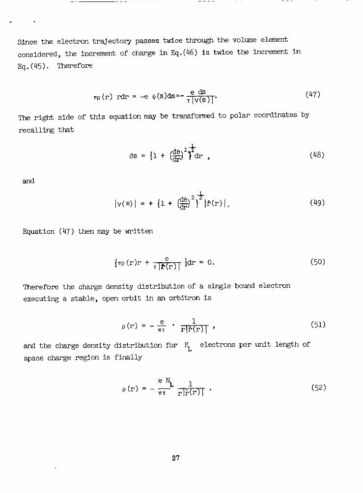
Since the electron trajectory passes twice through the volume element
considered, the increment of charge in Eq.(46) is twice the increment in
Eq.(45). Therefore
_p(r) rdr = -e ¢(s)ds =_- e dsIv(s)l"
(47)
The right side of this equation may be transformed to polar coordinates by
recalling that
2_(48)
and
Iv(s)i: + {i+ _ J_(r)l. (49)
Equation (47) then may be written
{ITp(r)r+ e }clr'= 0_l{"(r)I
Therefore the charge density distribution of a single bound electron
executing a stable, open orbit in an orbitron is
(5o)
p (r) - e . 1_ rig(r) I '
and the charge density distribution for
space charge region is finally
(51)
electrons per unit length of
(r)-e NL
WT(52)
27
T
is equal to --.2
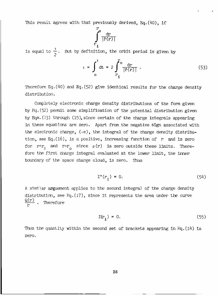
This result agrees with that previously derived, Eq. (40), if
r
r.1
But by definition, the orbit period is given by
• = dt=2
0 r.1
(53)
Therefore Eq.(40) and Eq.(52) give identical results for the charge density
distribution.
Completely electronic charge density distributions of the form given
by Eq.(52) permit some simplification of the potential distribution given
by Eqs.(13) through (15),since Certain of the charge integrals appearing
in these equations are zero. Apart from the negative sign associated with
the electronic charge, (-e), the integral of the charge density distribu-
tion, see Eq.(16), is a positive, increasing function of r and is zero
for r<r. and r>r since o(r) is zero outside these limits. There-i o
fore the first charge integral evaluated at the lower limit, the inner
boundary of the space charge cloud, is zero. Thus
I'(r i) = O.
A similar arguement applies to the second integral of the charge density
distribution, see Eq.(17), since it represents the area under the curve
Q(r) Thereforer
(54)
i) = O. (55)
Thus the quantity within the second set of brackets appearing in Eq.(14) is
zero.
28

It may be useful to emphasize several observations concerning p(r).At both the inner and outer turning points p(r) diverges since _(r i) =
_(r o) -- 0. However the integral of p(r) remains finite and it is generally
an integral function of p (r) that is required in the analysis. Perhaps
the most important property of _ (r) (because of its serious consequence)
is its form. The form of p (r) renders the Poisson Equation nonintegrable
analytically. Although this is a serious mathematical handicap implying that
a general solution to the problem is not possible, self-consistent particular
solutions having any prescribed accuracy can be developed using iterative,
numerical integration. _nese latter difficulties are the consequence of the
fundamental nonlinearity of the orbitron.
29
1.7 SELF-CONSISTENT SOLUTION (ist APPROXIMATION)
The analysis has now yielded all the information necessary
to develop a selgconsistent solution for the electron motion
in an orbitron: Eq. (14) gives the potential distribution for an
arbitrary charge density distribution; Eq. (26) gives the elec-
tron radial velocity for an arbitrary potential distribution;
and Eq. (52) gives the charge density distribution as a function
of the radial component of the electron velocity. These equa-
tions may be considered a set of consistent, simultaneous integro-differential equations. _(r) and _(r) may be eliminated by
substituting Eq. (26) into Eq. (52) and then substituting the
result into Eq. (14) which gives a single nonlinear, integral
equation in ¢(r) alone. This equation is not written heresince it is nonintegrable analytically; implying that a general
solution to the orbitron problem is not possible.
However, after having specified all pertinent parameters,a particular solution may be developed (one solution for each
set of parameters) by iterative, numerical integration. The
continuation of the analysis beyond this point therefore involves
a combination of both numerical and analytical techniques.
The starting point for obtaining a particular self_onsistent
solution using these methods is the radial velocity equation
(radial mode kinetic energy equation). The application of
numerical methods requires a knowledge of the specific range of
integration. Thus it is first necessary to establish the turningpoints (space charge boundaries). The ratio of the turning
points is, in general, given by Eq. (27) but for the presentneed it is more convenient to write it in the unconstrained
form (without the stability constraint which will be reinserted
later on) by substituting from Eq. (22) for E (r) and recalling2 othat the outer turning point kinetic energy T(ro), is given by
3O
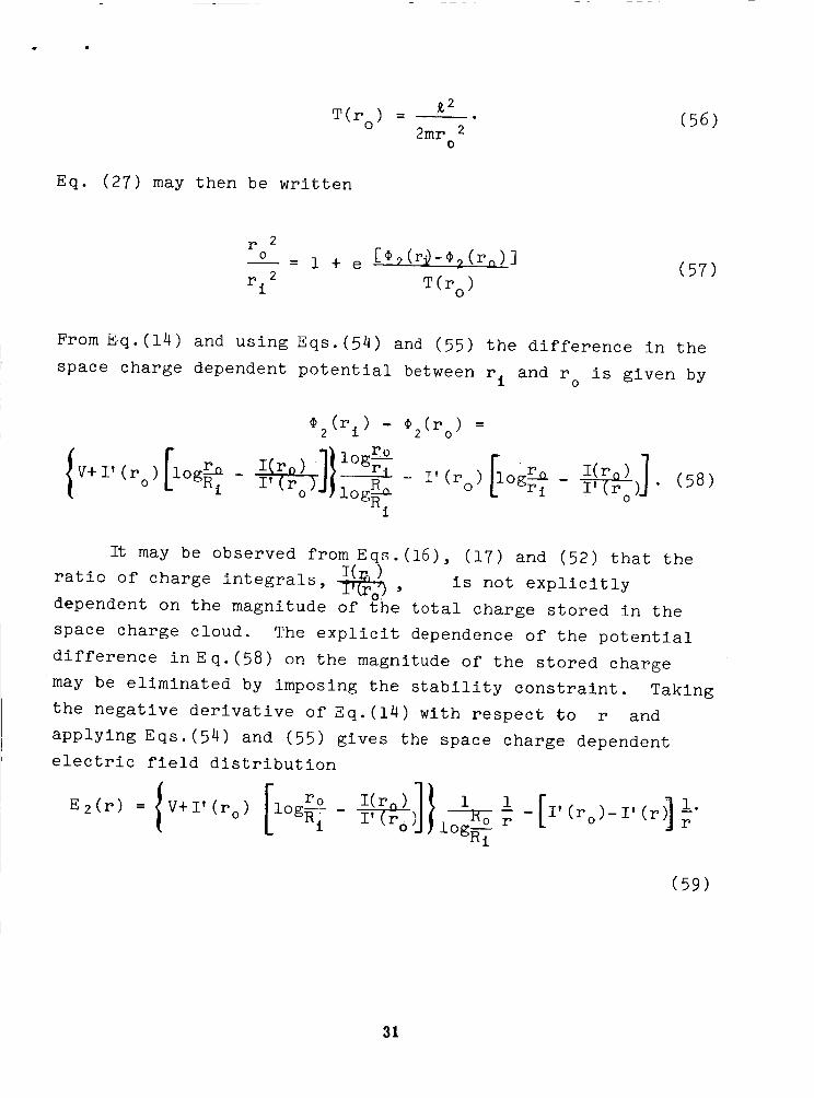
e, •
T(ro) =_2
2mr 2o
(56)
Eq. (27) may then be written
r 2
o - 1 + e [¢_(r_-¢2(rn)] (57)
ri2 T(r o )
From E q.(14) and using Eqs.(54) and (55) the difference in the
space charge dependent potential between r i and r ° is given by
'(r o) [log r° -[ R_
¢2(ri) - ¢2(ro) =
I!_rl _-_ - !' (r O) Ogr_ - :i,-(ro) j • (58)l°gRi
may be observed from Eqs.(16), (17) and (52) that the
ratio of charge integrals, • is not explicitly
dependent on the magnitude of the total charge stored in the
space charge cloud. The explicit dependence of the potential
difference in Eq.(58) on the magnitude of the stored charge
may be eliminated by imposing the stability constraint. Taking
the negative derivative of Eq.(14) with respect to r and
applying Eqs.(54) and (55) gives the space charge dependent
electric field distribution
l [ ro I(r____)]l 1 1 [i,(r )_I,(r_.E2(r) = V+l'(ro) l°g_ i - l,(re_ ---_o _ - o rl°g_-_i
(59)
31

Evaluating this equation at r e and substituting the results intothe stability criteria, Eq.(22), and using Eq.(56) to eliminate_2 in terms of T(r ) gives
o
a 2T(r ) = -FeE (r°o 2 )ro
o2e{-- -_- V+I'(r o)I1 I(ro) ]I i (60.)og_ I '(r o ) R_
l°gRi
From this equation it fol_ows that
'(r ° ) = V[l-2T_r°) log ]
ev R i .
[log roo I (r o ) ]
_i I '(r o)
(61)
Using this equation to eliminate I '(ro) in Eq.
the potential difference between r i and ro
(58) gives for
_2(r i) - ¢2(r ) =o
2T(r°) [i 2T(r ) R__] [!°g_ I_]Ilog r_ + V o log Ri [log I (royc_2e ri _2ev _ I!rIoi ] (62)
which does not depend explicitly on the magnitude of the stored
charge.
It is shown in Appendix E that optimization of the total
charge stored in the rotating electron cloud corresponds, in
part, to maximizing it with respect to r i. The maximization
32
of NL with respect to r i requires that r i = Ri. That isthat the inner turning point (and the inner boundary of the
space charge cloud) is displaced from the surface of the anode
only by a very small distance, sufficient to assure that theelectrons do not collide with the surface. In practice, this
distance may be of the same order of magnitude as the surface
roughness and therefore very small compared with Ri. Setting
ri=R i thus does not involve a substantial approximation and thedifference between them may be neglected in the analysis (see
AppendIY R ) Al*_ .... _ *_ condition is very important to the
optimization of the stored charge, it has other, equally import-
ant, consequences. Setting ri=R i reduces the system from a 6
parameter system to a 5 parameter system, but accomplishes the
reduction in a way which permits considerable additional analy-
tical progress without specifying all other parameters. Apply-
ing ri=R i to Eq.(62) reduces that equation to
¢2(ri)-@Z(ro ) - 2T(ro) ro [i 2T(ro) R ]log -- + V log ,(ri=R i),a2 e ri a 2 eV
(63)
and substituting this into Eq.(57) and rearranging gives the
following transcendental equation for the ratio of the outer
to inner turning points
where
ro e211 _log i + - + B=o, (ri- Ri),riJ
a2eV Ro
8 - 2T(r ° ) log Fi .
(64)
(65)
33

6 is not an independent parameter, but a specific function of
prescribed parameters. Thus the introduction of 6 does not
amount to introducing a new parameter since all the parameters
on the right side of Eq.(65) are prescribed parameters and
therefore specify 6. Alternatively, 6 may be considered a
subset label, specifying not a single particular solution but
rather an entire subset of particular solutions in which there
remains a considerable range of variation of the parameter on
which 6 depends, subject only to the condition that 6 remain
constant. 6 is here introduced as a mathematicl convenience,
however, in Appendix D its physical interpretation is discussed
and it is shown that 6 > 0 for all electronic charge distri-
butions and 6 may be considered a measure of the reduction in
electric field at the outer cylinder resulting from the space
charge insertions.
Eq.(64) gives the ratio of turning points in terms of
prescribed parameters only,which do not explicitly involve
the charge density distribution. Actually, since it has been
specified that ri _ R i and R i is prescribed, Eq.(64) gives the
outer turning point in terms of prescribed values of a2 and
B. This substantially reduces the number of self_onsistent
particular solutions for electron trajectories in the orbitron
since all solutions for which ri _ R i are rejected. However,
this is a considerable advantage since only those particular
solutions are retained for which the charge stored in the
electron cloud is optimized.
It is obvious that the space charge integrals l'(ro),
l(r o) and l(r) in Eq.(14) must apply to exactly the same
region of r-space as that to which _ (r) applied. The first2
approximation to these integrals is obtained by substituting
eNL . __i the space charge free _. Therefore theinto p(r) = _ r_'
34

ratio of the outer to inner turnin_ points in the space charge
free radial velocity equation, (where the subscript o
m X iloindicates that 8=0), ust be t_e same as the ratio of the outer
to inner turning points in the space charge dependent radial
velocity equation, (where the subscript B indicates any
value of 8>0 implying 8 101>0). Thus
(r°)o(re) (66)
isrio8=0 and
some value
a function of _2 only as may be seen from Eq.(64) for
(o_I is a function of both _2 and 8. I f _2 is82 o
applicable to Eq.(64) for 8=0 and e# is
_2 applicable to some prescribed value of 8>0,the value of
the only way Eq.(66) can be satisfied is if e2>_2B o"
Eq.(66), it follows that the set of equations
Thus, from
log r-_ + -- ' =2 r.21
rolog _ii + -_- r_
romust be solved simultaneously for --
ri
0 (67)
+ B = 0 (68)
and e_ for some pre-
scribed set (_,B). According _0 the stability criteria, the
2 is 1minimum value of s o _. This value of _2 strictly applies
only to a_ and not to _2o since the space charge free 9 is
used only as an initial generating function known to have an
approximately correct shape. However_ in this first develop-
ment of a self-consistent solution, the stability criteria is
applied to both a_ and _. This value of _2 corresponds
(_, yields the highestto the maximum value of r and thus
(allowed) probability that o electrons miss the launcher during
35

the first few orbits after injection. (_e Appendix E ). Fromro
Fig.l,where numerical solutions of Eq.(64) for r-_ as a
function of a 2 with _ as family parameter are plotted, it
may be seefi that
--2.59, ° : y). (69max
o
From Eqs.(66) and (69) and Fig.2, where is plotted as a
function of 8 for a_=l, it may be seenXtJa_ the maximum
value that may be prescribed for B is about 1.9. In this first
development of a self-consistent solution, a mid-range _ is
arbitrarily chosen such that
8=1.0. (70)
For this value of
follows that
8 and from Eqs.(66) and (69) and Fig.l, it
a_ = 0.684. (71)
These numerical values are needed for later computations.
The first approximation to the charge density distribution
is given by
-eNL i
_1 (r) = nT • _ , (72)o r9 o
where the subscript o indicates that the electrons have been
arbitrarily assigned the radial velocity strictly applicable
only to electrons in a space charge cloud which has a negligibly
low charge density. This does not imply that p1(r) is neces-
sarily small (N L in Eq.(72) may be large), but only that
Eq.(72) is an approximate relation which is to be refined in
36

ro
r i
6.0
5.0
4.0
3.0
2.0
1.0
0.4 0.5 0.6 0.7 0.8 0.9 1.0
2
Fig. I Numerical Solution of Eq. (64)
37

B
5
1
2 4 6 8 i0
B
Fig. 2
Note:
Numerical Solution of Eq.(68) for the Maximum
Value of aB2 (_ = I).
This value of _ allows the maximum range of
B constant with Eq.(66) and thus the maximum
range of N L .
38

subsequent iterations. From Eqs.(14) and (26), Eq.(72) may
be written in the following dimensionless form (after settingall charge integrals to zero),
i2 m--
• l F_ Ij,,, i
,-eNL) _{ 2 [ 2 }-_
o ro G o r o
_+_ i-_) drI 2_ log r 2 _ r2 ro
ri
(73)
The denominator of this equation has been integrated numeri-
cally and the equation is plotted in Fig.3 as fl(ao,+) for2_] -o
o-3' where
rorP.l(r )rfl(a or -r)
o l_-eNL_ "
The first approximation to the first charge integral
I {(r) is then obtained by substituting Eq.(73) into Eq.(16)
and performing a numerical integration, using Eq.(69) to de-
fine the lower limit of integration. The result is plotted
in Fig.4 as g_(_o,-_ -r ) (a dimensionless function obtained byi _" O eNL
dividing Eq.(16) by 2_e )'o
(74)
r, ) -eNLg'l(%'r o :
The first approximation to the second charge integral
l_r) is then obtained by substituting the numerical results
from Fig.4, Eq.(75), into Eq.(17) and performing the second
integration, again numerically. The results are plotted inr
) (a dimensionless function obtainedFig.5 as gl(aO,ro
(75)
39
6
o
0.4
Fig. 3
0.5 0.6 0.7 0.8 0.9 1.0
r
ro
1st Approximation to the Space Charge
Distribution
4O

I°o
v
1.0
0.9
0.8
0.7
0.6
0.5
0.4
O.3
0.2
0.1
Fig. 4
0.4 0.5 0.6 0.7 0.8 0.9 1.0
r
ro
Ist Integral of fl (a r )o' ro
41

0.35
I°o
hO
0.30
0.25
0.20
0.15
0.i0
0.05
............... j
0.4 0.5 0.6 0.7 0.8 0.9
Fig. 5 2nd Integral ofr
fl(_o ' ro
42

eNLby dividing Eq.(17) by - 2_E_),
o
r ) :_If(r) (76)gl (So ' r° .eN L •
2_c o
g' and g have been introduced as a mathematical convenience.
They are the same as I' and I except that they do not depend
explicitly on N..
Substituting these numerical results back into Eq.(14)
give s (77)
V iog R--£°Ro eN L I[1 Ro _ IOg_-IRo "o 1r og --Z-+gl(_ o I r
¢2 l(r ) = 2_eo r ' -gl (_-_-)
where the second subscript on #21(r) indicates that it is the
first approximation to the space charge dependent potential
In Eq.(77), Eqs.(54) and (55) have been applieddistribution.
and the result
gi(%,l) = 1 (78)
has been used.
The first approximation to the electron radial velocity
as a function of the space charge dependent potential distrib-
ution is obtained by substituting Eq.(77) into Eq.(26), then
using Eq.(61) to eliminate NL after having substituted the
numerical results of Figs.4 and 5, Eqs.(75) and (76), into
Eq.(61). The result of these operations is
43

(79)
_2 4T(ro) ro r2 og _f_ + gl o,_jo )_g1(a ,I)log T + ..._._ + _ _--- o
1 = Ct_ m r 0
log ri gl(_o,l)
Tt may be seen that rl does not depend explicitly on N L. This
completes the development of the first approximation to a self-
consistent solution of the electron motion and distribution in
an orbitron (except for several detail calculations which are
made later).
The second approximation to the charge density is obtained
by substituting Eq.(79) into Eqs.(52) and (53) which gives
r
{ _2___(I r_ } [log ___ro+gl(_-_o)-gl (_i) ];r r 02(r) log _+ - 8[l-_g ro_go _T i(%,i )
(-eNL)-/12_. log -r-+2r° _A_/_kl__-_)+r2°' _log r_a+gl(ao_el)-gl(ao,l_d_80)ro]_ I_o
i log _i-g l(adl)
The denominator of this equation has been integrated numeric-
ally and the equation is plotted in Fig.6 as f2(gl,a ,B,rr--)8 o
where
r ror °2(r)
f2(gl'aB'B'-r°)- (- eNL)2_ ' (81)
The functior _2(r),which does not depend explicitly on N L.
Eq.(80), may now be used in the same way as above to begin the
second iteration and thus generate the second approximation to
r__) andthe dimensionless charge integral functions g_(gl,aB,B, ro
44

6
A
ao.
e_
N)
c,4
1
0
\
tl
0.4
\
\
, I I I I I
0.5 0.6 0.7 0.8 o.9 1.0
r
ro
Fig. 6
Note :
2nd Approximation to the Charge Density
Distribution.
The ist approxlmatlon, f1(a r ), is- 0 _ rshown dashed for comparison, o The rela-
tively small difference between fl (_ r )
and f2(gl, aB,B,___) implies that the °" r-_
iteration process o converges rapidly.
45

r ). These functions may then be used, in the samegz(gl,_ _,-o
way as above, to generate the third approximation to the charge
density distribution, p3(r) may now be used to begin the third
iteration, and so on... The development of a self-consistent
solution having the required accuracy is finally completed if
the result of the last iteration Pn(r) differs from the re-
sult of the previous iteration 0n__1(r), by less a prescribed
amount over the entire range of the electron motion (ri!r!ro).
From a study of the form of Eq.(80), it is clear that the charge
boundaries in p_r) will be the same as they are in o2(r).
Thus, no further adjustment in =8 and _ will be required in
subsequent iterations.
At this point, the first approximation to the number of
electrons in unit length of the rotating electron cloud, (NL) P
may be obtained immediately from Eq.(61). Using Eqs.(75) and
(78) to evaluate the left side of this equation, eliminatingRo
log _ii on the right in terms of 8 from Eq.(65), and sub-
stituting for I'(r_ and I(r o) on the right from Eqs.(75) and
(76) gives (after rearrangifig)
(NL) 1 =_2 e2[!og ro )]
B r i - gl (_I
(82)
All the parameters on the right side of this equation are pre-
scribed except gl (ao, l ), the value of which has already been
calculated. Substituting into Eq.(82) the numerical values of
the prescribed parameters given in Eqs.(69),(70)and (71) , and
the numerical value of _ (=o,i) from Fig.5 gives
(NL) I =
toT(r o )
(0.422) e 2
(83)
46

50 eV is about the minimum outer turning point kinetic energyconsistent with an acceptable ionization probability (for most
gases). The inner turning point kinetic energy is given by,
from Eqs. (20) and (56),
[ro@T(r i) = _9_ij T(_) , (84)
which from Eq.(69) yields T(ri) = 6.7 T(r_. From this result,
it is clear that the minimum acceptable T(_ ) should be used
to avoid the penalty of a reduced ionization probability in the
neighborhood of the inner turning point. The outer turning
point kinetic energy is therefore prescribed such that
T(r o) = 50 eV. (85)
Substituting this value into Eq.(83) gives the first approx-
imation for the number of electrons per unit length of the ro-
tating electron cloud (for Ri = ri,a _ 1= _, B = i, T(r o) = 50eV).
(NL) I = 0.825 x 109 cm -l. (86)
Referring again to Fig.6, it can be inferred that the
_r_r) which will result from the secondfunction g2(gl, a B, B, ro ,
iteration, has the property g2<g . Combining this with1
Eq.(82) implies that the second approximation to N L will yield
a number which is smaller than (NL)I, since the denominator of
Eq.(82) will increase. Thus, it may be concluded that
However, since gl
(NL) 2 < (NL) I.
is only of the order of _ ofr o
log _ii
(87)
and
47

the difference between gl and g2 should not be large,
(NL) 2 probably will not differ substantially from (NL) 1.
The method of deriving a self-consistent value for the
ratio of the electrode radii is discussed in the following
paragraph. The Hamiltonian, H, of an orbiting electron is
simply its total energy. Therefore,
H = T(r) + U(r), (88)
where U(r) is the electron potential energy, given by
U(r) = -e_21(r),(89)
and thus
H = T(r) --e@21(r). (9O)
Since the Hamiltonian is constant over the entire electron
trajectory, it may be evaluated at any point along the tra-
Jectory. However, it is convenient to evaluate H at the
outer turning point. _21(ro) is given by Eq.(77) after eval-
uating at r=r o. Substituting Eqs.(75),(76) and (78) into
Eq.(61) and using the result to eliminate NL in _21(ro)
gives
2T(ro) R o
_21 (ro) - a_ e log _i"
Substituting Eq.(91) into Eq.(90) gives (after rearranging)
log
(91)
(92)
48

R o
Thus, instead of prescribing _-- (which is equivalent to pre-
scribing R° r oo is already prescribed) it is prefer-N_i since R-_
able to prescribe H, since it is one of the more important
physical parameters concerning the dynamics of the electron.
For example, suppose that H_T(ro): From Eq.(92), it is ob-
vious that the outer turning point then occurs at Ro, the
surface of the outer cylinder. For certain applications, it
may be preferable to operate the orbltron in this mode.
However, for rn_Ro_ (actually_ ro=Ro-_', where.........a' _ _ma]l
compared to Ro) , it is probable that a large fraction of the
orbiting electrons could be collected at the outer cylinder.
This condition should be avoided in both ion gages and ion
pumps. Therefore, H should be sufficiently small that it is
improbable that electrons can reach the outer cylinder. This
occurs for H=0, which implies that if all the outer turning
point kinetic energy (angular mode) were converted (in an
elastic collision) to radial mode kinetic energy (an improb-
able event), the electron would reach the outer cylinder as
r_0. Thus, setting H=0 in Eq.(92) and using Eqs.(69) and
(70) (and recalling that it has been prescribed that ri:R i)Ro
gives -- = 3.65. This is the minimum value that may be pre-Ri Ro
scribed for -- (See Appendix E). From the above discussion,R i
it may be seen that to completely avoid the possibility of elec-
trons reaching the outer cylinder, a negative energy must be pre-
scribed for H. It is convenient (although somewhat arbitrary)
to prescribe
H = -T(ro). (93)
Substituting this into Eq.(92) gives
Ro 2 (94)log ro B '
4g

and using Eqs.(69),(70) and (71) yields the ratio of the elec-
trode radii,
Ro
_7. : 5.13. (95)1
The only way this number can be increased is to decrease
(prescribe a larger negative value).
H
The method of deriving the self-consistent anode poten-
tial is described in the following paragraph. From Eq.(65),
after substituting from Eq.(94) and recalling that ri=R i ,
the self-consistent anode potential is given by
eV -2T
2(ro)(_ _ + B + log _o.).
1
Using Eq.(68), this may be written in the form
)r!eV -- T(r o
r 2
i
- H.
(96)
(97)
Using Eq.(93), this equation becomes
eV--T(ro) r[_21 + i_ (98)
Substituting into Eq.(96),(97), or (98) (which are s lmply dif-
ferent forms of the same statement) from the numerical values
given in Eqs.(69),(70),(71),(85) and (93) gives the self-
consistent anode voltage
V = 385 volts. (99)
5o

The method of deriving the launcher bias voltage is de-
scribed in the following paragraph. The electrons may be in-
serted into orbit at any point along their trajectory, however
at the turning points only a fraction of the space occupied by
the launcher need protrude into the space occupied by the elec-
tron trajectories, but if the launcher is located at any other
point along the electron trajectory the entire launcher is
within the space charge cloud. Thus, orbit insertion should be
accomplished at either the inner or outer turning points. At
either turning point, there are two principal methods of in-
serting the electrons into orbit: (i) The electrons may be accel-erated within the launcher, which iS biased to the local space
charge dependent potential, such that they are emitted from
the launcher with the prescribed turning point kinetic energy
(angular momentum) and with their velocity vectors coincidingwith the e-direction. (2) The electrons may be emitted from
the launcher with negligible kinetic energy, but constrained to
move in the e-direction only, from a launcher which is biased
below the local space charge dependent potential such that theyare accelerated up to the prescribed turning point kinetic
energy by the local field as they leave the launcher. It is,of course, possible to combine the two methods. The first
method is, in principle, more flexible and the accurate control
of the launch (insertion) parameters is simpler and more posi-tive. Of the two turning points, the more suitable location
for the launcher is the outer turning point, ro, since thislocation gives the lowest probability for electrons collid-
ing with the launcher on subsequent passes (for moderate tohigh eccentricity trajectories). For electrons emitted from
a launcher at ro, in the e-direction, and with kinetic
51

energy T(r o) (_=[2 m ro2 T(ro)]½), the launcher bias voltage
must be such that it matches the local space charge dependent
potential ¢21(ro). From Eqs.(77),(61),(75),(76),(85),(92) and
(93), it follows that the launcher bias voltage is given by
eV b = e¢21(r o )i
= 2 T(ro) , (lO0)
or
Vb = i00 volts, (i01)1
where the subscript b I indicates that this bias applies to
the first launch method. (It is interesting to observe that
for a space charge free potential distribution, and all other
parameters held fixed, the local potential would be _160 volts.)
If the electrons are emitting with negligible kinetic energy,
the launcher must be biased such that
eE¢21(ro) - Vb] : T(ro) , (102)
from which it follows that
Vb2= 50 volts, (103)
where the subscript b 2 indicates that this bias applies to
the second launch method. (For a space charge free potential
distribution, the required bias would be -- ii0 volts). In the
second launch method, the application of the correct bias to
the launcher is not sufficient to assure that the electrons are
correctly inserted into orbit since the potential difference
52

through whichthe electrons fall depends on the direction which
the electrons leave the launcher since the potential hill sur-
rounding an acceleration-biased launcher is not symmetrical,being steeper on the inside (toward the anode) than it is on
the outside. The acceleration-biased launcher cannot be located
at r o (the outer turning point) since the electron must
arriveat r o with r(ro):0 and at this point have kinetic
energy T(r o) (a prescribed parameter). The only way that anacceleration-biased launcher can satisfy these conditions is_ *_ _* .... to be _-_........... _,_o _._±_ed from the launcher in a direction
which makes an_angle somewhat less than with the radius vec-tor (emitted'outward) such that the electrons pick up angular
momentum and kinetic energy in falling down the potential hill.
The electrons then continue to coast outward (against the field)
until the radial component of the momentum goes to zero. This
point is ro, however for insertion into the correct orbit thelauncher bias and the direction of emission must have been such
that the electrons arrive at this point with the proper angular
momentum (_=[2 m r_ T(ro)]½, wher_..... T(ro) is prescribed, say
50 eV). The important conclusion is that an acceleration-biased
launcher is completely within the space charge cloud since the
cloud outer boundary (trajectory outer turning point) is well
outside the launcher location. A similar argument applies to
acceleratlon-biased launcher locations in the neighborhood of
the inner turning point and a similar conclusion is obtained.
It is obvious that a potential hill 50 volts high produces a
substantial perturbation in the space charge dependent potential
distribution. It is not only a large perturbation locally, but
it is non-negliglble over a substantial fraction of the volume
of the space charge cloud in the z-neighborhood of the launcher
since its decay is quasi-logarithmic. It thus appears that the
53

only acceptable method of launching is the first, with launcherlocations restricted to either the inner or outer turning points,
since this method produces no perturbation of the space charge
dependent potential distribution, and only a fraction of thevolume of the launcher protrudes into the space charge cloud
volume.
Under certain conditions, the orbitron principle con-
tains a natural feedback mechanism which may be used to main-
tain the number of electrons in the space charge cloudconstant. This feedback mechanism is discussed in the follow-
ing paragraph.
Suppose the electrons are inserted into orbit at the
outer turning point with kinetic energy T(r o) from a launcherbiased to match the local space charge dependent potential.
Thus, the outer turning point is fixed at r ° (the launcher
location), the electron emission angle is fixed at -_ (withrespect to the radius vector), and the electron emission
energy, Te , is fixed since
Te = T(ro). (104)
Now, suppose that the electron injection rate into the space
charge cloud is perturbed such that it exceeds, by a small
fraction, the total electron loss rate from the cloud. It
necessarily follows that NL must begin to increase. Theimmediate effect of increasing NL is to lower the potentialdistribution within the space charge cloud, see Eq.(77).
Thus, _ 21(ro) must decrease or, considering the potential a
function of NL, it follows that
54

¢ 21(ro, NL + ANL) < ¢21(ro, NL). (105)
Since r i = Ri+_ (and _ is negligible), the potential atthe inner turning point is nearly identical with the anode
potential and is, therefore, constant. Thus, at the inner
turning point, the potential must satisfy
¢21(ri, NL+ANL) = ¢21(ri, NL). (lO6)
............. _ ............ ._._,,_= _±±_ in the numerator
of Eq.(57), which gives the ratio of the turning point radii,
must increase as N L increases. Now, concerning the denom-
inator of Eq.(57), before the injection rate perturbation,
the launcher bias must satisfy Eq.(100), that is
Vb = ¢ 21(ro , NL),1
(io7)
and after the perturbation begins, the launcher bias is
greater than the local space charge dependent potential since
the bias is fixed and the potential at the outer turning point
decreases as NL increases, see Eq.(105). Thus, the elec-
trons are emitted from the launcher into a retarding field.
The outer turning point kinetic energy, after the beginning
of the perturbation of the injection rate, is given by
= (r ° NL÷ANL)]T(r o, NL+AN L) T e -e[Vbl-¢21 , (108)
which may be written, using Eqs.(104) and (107)
T(r o, NL+AN L) = T(ro,NL) -e[¢21(ro,NL)-¢ 21(to , NL+ANL)].
(109)
55

• p
From this equation and Eq.(105), it is obvious that
T(r NL+AN L) < T(ro,NL)-O'
(iio)
Thus, the perturbation which increased NL, resulted in a
decrease of the outer turning point kinetic energy. Using
Eqs.(106) and (109) to evaluate Eq.(57) after the beginning
of the perturbation gives
r 2
° I = 1 + e
NL+AN L
[¢ 21(ri,NL ) - ¢ 21(ro , NL+ANL)3
, (ro,NL)-¢z/ro NL+ANL)]T(r o N L) - e[¢21
.(lll)
From Eq.(105), it follows that increasing NL by AN L has
increased the numerator and decreased the denominator of the
term on the right in Eq.(lll). Therefore, it follows that
r 2 r 2
r 2 r
iNL+AN L NL
(112)
and since r ° is fixed, it necessarily follows that r i
must decrease. But decreasing r i implies that electrons
collide with the anode, since ri=R i. These collisions
increase the total electron loss rate from the space charge
cloud which produces a decrease in NL (and incidentally a
decrease in the mean orbiting llfe time). It is, therefore,
concluded that the variation in the space charge dependent
potential distribution as a function of N L is such that it
has the effect of closing a feedback loop around NL and
tends to hold N L constant (provided, of course, that the
orbit injection parameters, electrical parameters, and geo-
metrical parameters all belong to a self-consistent set).
56

1.8 ION PRODUCTIONRATE
The average number of ions produced in unit time by
the electrons in unit length of the rotating space charge
cloud, (N+)L' is given by
(N+) L=<V>NLno+, (113)
where o+_
<V> -
gas ionization cross section for electronsm
having a mean kinetic energy <T> = _<v> 2,
mean electron velocity,
n _ gas member density.
NL has already been calculated and o+ has been repeatedly
measured for many gases by numerous experimenters and is
available in the literature. Thus, it remains to calculate
the mean electron velocity, <v> .
There are several useful definitions of the mean elec-
tron velocity, each differing slightly from the others. The
definition of <v> considered most useful in this applica-
tion is that electron velocity properly associated with the
mean radial position of the electron, <r> . Therefore, it
is first necessary to derive a self-consistent expression for
<r> , then evaluate it for the particular set of parameters
under consideration in this first self-consistent solution
and, finally, compute the electron velocity at this mean radial
position, that is to compute v(<r>).
The second approximation to the mean radial position of
the electrons is given by
57

1 f_< r_>- rJ1 r dt0
ro
2 _ r dr
r°_1_i; _i
Integrating by parts gives
(i14)
r
lrf lr°-f°drfr.
r i
(115)
Equations (53) and (54) may be used to evaluate the first
integral, with the result
ro
<r> f2 dr -_-o : i r_ 1 rl
r.1
The second integral may be written, using Eqs.(52), (79),
(80) and (81), as
(116)
ro
%> r dr< = i- _oo f2(gl ' _B' B'-_o) _oo ' (i17)
ri
and from an equation similar to Eq.(75), but applying to the
2rid approximation to the charge integral l'(r), Eq.(ll7) may
be written
ro
--_o ff r dr'x >= I- g'2(gl'aB'B'r--_ ) _oo "
1j
This integral has been evaluated numerically (for _ = --o 3
8=1, ri_R i) and the result is
(118)
B8

<r____>_- i - 0.254r o
= 0.746. (ll9)
The electron velocity at any point along its trajectory
is given by
1(120)
v(r) = {_2 + r 2 _ 212
and using Eqs.(20) and (56), thls may be written
1
2T(ro) to2 t2"v(r) = {_2 "I" 7- r 2
(121)
and substituting for
tion to the electron velocity
i
V 2(r) = m {I + =_
from Eq.(79) gives the 2nd approxima-
1
r if[aog +g{_o-)-g_(_o 1)],r o
ro
[log ri _ (_o,i)]
(122)
Evaluating this expression at <--_e> given by Eq.(llg), taking
r>)r° from Eq (69) B from Eq.(70), _8 from Eq.(71), g_<-ro
r i
from Fig.5, and gl(_o,l) from Fig.5, yields
1 1
<v,> v,(<_r--->) (2 38)._ 12T(r°)] _0
(123)
Digressing for a moment, the electron mean kinetic energy
may be immediately calculated from Eq.(123), slnce
59

m 2 (124)<T> = _ <v> ,
which gives
<T> = 2.38 T(r ), (125)o
and substituting from Eq.(85) for T(r o) gives
<T> = 119 eV. (126)
Thus, for the set of parameters chosen, the electron mean
kinetic energy is about the center of the kinetic energy
ran&e corresponding to the ionization probability maxima for
a large group of common gasses. From Eqs.(85) and (123), it
follows that the mean electron velocity is
<v2>= 6.45 x 10⁸ c__mmsec. (127)
Returning now to the ion production rate (Argon is
used throughout as a typical gas wherever gas properties are
required in detail calculations) given by Eq.(ll3) and taking
N L from Eq.(86), <v2> from Eq.(127) and the ionization prob-
ability for Argon (the average of many values from the litera-
ture applicable to Eq.(126)) as
16
OAr + = 3.8 x i0 -_ cm 2(128)
yields
(NAr+)L = 6. 6 x I018 PT' I Ar+ (129)
60

for each centimeter of space charge cloud (the T-subscript
on PT indicates that pressure is measured in Torr). Thisresult should be considered a first approximation since the
value of NL used is a first approximation even though thevalue of <v > is a second approximation. The ion current
2
produced (per cm of space charge cloud) is simply e(_Ar+) L(-e _ electronic charge), and from Eq.(129) this is
(JAr+) L = 1.06 PT' (Amp). (130)
The electron injection rate required in two typical
modes of operation is computed in the following paragraphs.
One of the simplest modes of operation is that in which the
electrons drift slowly away from the launcher (in the z-
direction) until they reach z=L where they leak out of the
coaxial cylindrical structure through a weak mirror field.
This mode of operation tends to minimize the x-ray induced
residual current since the electrons which do not collide
with a gas atom are eventually collected outside the orbitron
structure. Suppose that the potential of the mirror electrode
is such that the mean velocity in the z-direction is <Z>.
Thus, the current leaving the neighborhood of the launcher in
the z-direction is -eNL<Z > (none of which returns). There-
fore, the electron injection rate required to maintain N L
constant in the neighborhood of the launcher is
e = NL <_ > " (131)
It is assumed that the electrons are inserted into orbits
which are sufficiently eccentric to miss the launcher during
the interval of time required to drift out of the z-nelghbor-
hood of the launcher. For a l.auncher biased to match the local
61
space charge dependent potential, this may be of the order
of five orbit periods (or more). However, for an acceleration
biased launcher, this interval is probably of the order of one
orbit period. Thus, <Z> must be larger (in this mode of opera-
tion) for an acceleration biased launcher than for a potentialmatched launcher. This implies that the electron injec-
tion rate must be larger for the acceleration biased launcher
than for a potential matched launcher.
For a potential matched launcher, the electrons must move
a distance aZ=L' (L' is the launcher length) in a time inter-
val of the order of 5_. This yields the approximate relation
h' . (132)<v> l_<r>
For L'=0.5 cm
R =2.5cm(implying from previous results thato
gives
= io, .min
(a small but yet practicable value) and
<r>= 0.94 cm)
(133)
This constraint places an upper limit on the parameter
Np_ somewhere in the neighborhood of an10 3 . For acceleration
biased launcher, this upper limit would be smaller since<Z>
Eq.(133) gives a larger minimum value for(V>
An important mode of operation involves a relatively
strong mirror field at Z=L such that all electrons are re-
flected. By properly restricting the maximum value of operat-L <v >
ing pressure, the ratio R' and <-_, NL may be maintained
approximately uniform over _he full range of Z (this was not
necessarily the case in the previous mode of operation). For
6B

where a+ _ ionization collision cross section of the
atom for electrons having a mean kinetic
energy <T> .
The number of non-ionizing collisions per unit time is there-
fore
_-_ = <v> L N L n(o-o+). (136)
This &iso may be taken as the number of elastic collisions
per unit time, since the excitation cross section is generally
very small compared to a _ In some fraction of the elastic
collisions, there is sufficient electron kinetic energy loss
or momentum change such that the electrons are left in an un-
stable orbit after the collision and, subsequently, collide
with the anode. The number of electrons lost from the space
charge cloud in unit time by this mechanism is therefore
h Ve = h( v-v+ ) = <v> L N L nh(a-a+) , (137)
where h is in the interval 0 ih!l, the exact value of
which is not essential.
A small fraction of the electrons orbiting in the z-
neighborhood of the launcher, continuously collide with the
launcher. The electron-launcher collision frequency is worked
out below for a launcher located at r and biased to matcho
the local space charge dependent potential (the necessary pro-
cedural modifications for treating the acceleration biased
launcher are rather obvious). Consider a cylindrical launcher
of radius RL, the axis of which is parallel to the orbitron
axis and located at r ° (electrons are ejected from a central
slit, parallel to the launcher axis, which is orthogonal to
the radius vector passing through the center of the launcher).
63

Obviously, the launcher radius should be as small as practic-
able. From practical considerations of the operations In-
volved in the assembly of the various launcher electrodes, anear minimum launcher radius is considered to be
RL = 0.05 cm. (138)
The effective launcher length, L', protruding into the end of
the space charge cloud, is taken as
L' = 0.5 cm. (139)
The electron collision frequency with the launcher is given
by
where ALe
1 _I (r) dA, (140)Je
A L
that part of the launcher projected area onto a
radial plane passing through it,which is within
the space charge cloud,
The current density is given by
Je(r) _ p(r) Ve(r) . (141)
But since R L << r° and
in the neighborhood of
that
Ve(r) is a slowly varying function
r , the approximation may be madeo
Ve(r) _ Ve(_) , ro-RL_r_r o. (142)
64

a launcher biased to match the local space charge dependentpotential, electrons that collide with the launcher have a
kinetic energy of 50 eV (for a launcher located at the outer
turning point). If the launcher were located at the inner
turning point, the electrons would collide with a kinetic
energy of 335 eV, which is another reason for avoiding aninner turning point location for the launcher. The electron
launcher collisions produce soft x-rays, a fraction of which
radiate from the launcher to the ion collector surface (outercvlinder] wh_e they _+ _+........ _ _oelectrons. Thus, in this mode
of operation, it is necessary, in the interest of reducing the
residual current for ion gage applications, to separate thatportion of the outer cylinder which surrounds the launcher
from the remainder of the outer cylinder and use only the
latter for ion collection. This substantially reduces the
photoelectron emission from the ion collector, since the sub-
stantial fraction of the soft x-rays and photoelectrons leavethe surface in a direction near the surface normal and thusdo not reach the ion collector.
Under the above conditions, the total number of elec-tron-atom collisions in unit time is
_ = <v>L NL no , (134)
where o e total collision cross section of the atom for
electrons having a mean kinetic energy <T> .
Similarly, the total number of ions generated in unit timeis
= <v> L NL no+ , (135)
85

From this approximation and Eqs.(124) and (125), the current
density may be written
<V>
j0(r) -- _ 0(r). (143)
Substituting this back into Eq.(140) and taking p(r) from
Eq.(52) and noting that dA=L'dr, the electron-launcher col-
lision frequency becomes
<v> L,NL --[ro drVL - _ _ _ j r _(r). (144)
ro-R L. • DI _
'The strong variable in this integrand is r(r) since r ÷ ®
as r + ro Further r - R L _ r which implies that the range" O O
of integration is sufficiently small that r may be set equal
to r and factored out of the integrand. From Eqs.(71),o
(94) and (138), and taking
R =2.5cm,o
(145)
it follows that
r m
o RL = 0.96 r o,(146)
and that
ro
= 1.26 cm (147)
Therefore Eq.(144) may be written
66

ro
<v> L'N L / dr (148)VL = _ _ T r o r(r) "
ro-R L
Using Eq.(53) and Fig.4 to evaluate this expression, the
electron-launcher collision frequency is
<v> L'NL(O.185)
= r ' (149)o
and from Eqs_139) and (147)
vL =7.58 x i0 -3 <v> NL (15o)
The total number of electrons lost per unit time from the
space charge cloud by elastic, inelastic and launcher colli-
sions, is the sum of Eqs.(i35), (137) and (150). A necessary
condition for maintaining N L = constant is that the electron
launcher rate, Ne' must be equal to this loss rate. Therefore
N = <V>NL_Lno[(l-h)_ °-!++ h] +7 58 x i0 -3e O 'I.(151)
At low pressure (small n) the dominant term in this expression
is obviously the last term. Thus, maintaining N L constant at
low pressures requires a constant electron launch rate, inde-
pendent of P. This launch rate is given by
Ne = <V>NL[7'58 x i0-3], (152)
dropping all but the last term in Eq.(151). Substituting from
Eqs.(86) and (127) for NL and <v>, implies that the emission
67

current (required to maintain the total charge in the rotatingelectron cloud constant) is
= 0 645 ma, (153)i e
(again, for the specific set of parameters used in this first
development of a self-consistent solution). The pressure above
which the electron launch rate (required to maintain NL= const.)depends on P , may be evaluated by determining that pres-sure above which the last term in Eq.(151) is no longer domin-
ant (suppose it is only of the order of 90% of the total).Thus
-38.5 x i0
nmax< L_[(l-h) _-_ + h] ' (154)O
and again taking Argon as a typical gas, for which
and from Eq.(128)
OAr = 9.5 x 10 -16 cm 2
OAr +
OAr- 0.4, and taking
, (155)
L = l0 cm, (156)
gives the pressure above which the launch rate required to
maintain NL= const, is dependent on pressure
(PT)max
2.64 x 10 -5 Torr, (h=l), (157)
6.6 x I0 -5 Torr, (h=0).
68

A reasonably accurate estimate of h is a rather laborious
computation which involves not only quantum collision mech-
anics but also the specific geometrical parameters of the
orbitron, the space charge dependent potential distribution,and the electron trajectory parameters• The computation of
h is not done here, but from Appendix A, it may be seen that
h+l as _B2_ and that h÷hllml t as _2_1. Although
hllmlt>0 for all useful electron kinetic energies•
mh_ _m_+=_ . P may now be calculated from Eqs(135) and (152), whic_ e Tglves
N+ L n o+
NePT 7.58 x 10⁻³PT
and taking L from Eq.(156) and o+ from Eq.(128)
(for Argon), gives
(158)
NAr+ = 1.63 x 10⁴ , (Torr -I) •
NePT
(159)
The ionic pumping speed, S+ , associated with the ion
production rate is given by
v+
S+ = C± n '(160)
where Ci _ ion capture probability at normal incidence for
ions having kinetic energy T+(Ro)=e¢21(<r>), (=170 eV)•
69

Substituting Eq.(135) into Eq.(160) gives
S+
C±- <V> L NLO+, (161)
and using Eqs.(86), (127), (128) and (156), gives the ionic
pumping speed for Argon
SAr+ cm 3- 2 x 10³ . (162)
C± sec
The rotating electron cloud corresponds to a circulating
current which is given (approximately) by
<v> L (163)i8 = eNL 2_<r>
Thus, the ratio of emission current to circulating current is
given by, from Eqs.(152) and (163),
ie =.--- (7 58 X 10 -3 ) 2w<r>" L '(P<Pmax)' (164)18
and using Eqs.(ll9), (147) and (156) gives
ie
i 8- 4.47 x 10 -3 . (165)
This result validates the use of the time-independent contin-
uity equation, an assumption made earlier in deriving the
charge density distribution, see Eq.(29).
70
It was assumed earlier that the charge distribution is
nearly uniform along the Z-axis. The validity of this assump-
tion may be determined for the maximum pressure for which the
orbitron response is a linear function of emission current,
Eq.(157). The electron mean free path in Argon is given by
k(e,Ar) -OAr
0.032
and substituting (PT)ma x for PT from Eq.(157), gives
k(e,Ar)Imin= 5.8 x 102cm, (h=O).(167)
The distance traveled by an electron along its trajectory
during one orbit is of the order of
s = /2 _ <r> , (see Appendix C), (168)
and using Eqs.(llg) a_d (147) gives
s = 5.0 cm. (169)
Thus, in one mean free path, an electron executes
_(e,Ar)= 116 orbits, (170)8
which is adequate to assure nearly uniform charge distribution
along the Z-axis since in this number of orbits the electron
could have traversed the full Z-range several times.
71

This entire orbitron analysis has been based (in part)on the working hypothesis that the space charge was com-
pletely electronic. The validity of this hypothesis may bedetermined by calculating that pressure above which the
ionic component of the space charge is no longer negligible.
Since the mean radial position of the electrons is <r> ,the most probable radial position at which ions are formed
is also <r>. The mean ion llfe time, <T+>, is thereforethe time required for an ion to traverse the distance from
<r> to Ro. The ionic acceleration is given by
"" er - E(r). (171)
m+
Integrating this equation gives the ionic velocity
r
1
[_n+z ¢2l(<r>)-¢2l
m+/ [¢ (<r>)-¢21 31
I
(r)] Y, <r>_<r _<ro,
1
(r)] _ r o < r < R o,, _ - (172)
where the initial ion velocity is assumed negligibly small.
Integrating this result again gives the mean ion llfe time
ro R173)
/m+\7 dr dr
<T+> : "'--_2-el [¢21(<r>)_C21(r) ] _[ [¢21(<r>)_¢al(r) ]
<r> r °
¢21(r) is given by Eq.(77), and from Eqs.(15), (54), (55),
(75), (76) and (78), it follows that
Ro
IveN[2oro ]ll°gTlog _ii gl(e°'1) Ho" (174)¢31(r) = log Ri
72

Making the appropriate potential substitution in Eq.(173),
taking the limits of integration from previously defined_r ) from Fig. 5, and performing
parameters, taking g1(ao, rothe indicated integrations numerically, gives
Ifm+ V
<'[+> = 1.45 Ro _2 eVl "(175)
Taking R from Eq.(145) ando
Argon ion life time is
V from Eq.(99), the mean
<tAr+> -- 8.4 x 10 -7 sec.(176)
The number of ions in unit length of the interelectrode
space is given by
(N+)L = (N+)L <T+>. (177)
Substituting from Eq.(129) for (NAr+)L
for <TAr+> gives (again for Argon)
and from Eq.(176)
(NAr+)L = 5.5 x 10¹² PT" (178)
For the space charge to be considered completely electronic
(as has been done in the analysis)
(NAr+) L << NL.(179)
'73

Therefore from Eqs.(86) and (178), it follows that
PT I << 1.49 x 10 -4 Torr.msx
(180)
This result implies that the space charge may be considered
completely electronic below about 1.5 x 10⁻⁵ Tort. There-
fore, from Eq.(157) (for any value of h ), it follows that
over the entire linear dynamic range of the orbitron, the
assumption that the space charge is completely electronic,
is valid.
74

1.9 CONCLUSIONS
The development of the ist approximation to a self-
consistent solution for the electron motion, charge density
distribution and charge dependent potential distribution in
an orbitron, used the following assumptions:
0. The space charge is completely electronic.
i. The charge density distribution is sufficiently
uniform in the Z-dlrection that its variation
with Z may be neglected.
. The charge density distribution is independent
of e .
, Allowed orbits are members only of the orbit
subset which satisfies the stability criteria;
excluding, however, although members of this
subset, that part of the discrete series of closed
trajectories for which n is small.
, The time dependent component of the charge den-
sity corresponding to the collision loss rate and
the balancing injection rate is negligible, com-
pared to the equilibrium charge density.
These assumptions are shown to be valid for practicable config-
urations and modes of operation.
75

Under these assumptions, the consistent set of differen-
tial equations describing the space charge dependent potential
distribution, the charge density distribution, and the electronradial velocity are:
d (r de) _ r p(r)dr d-r e0
(Poisson Equation),
d [r r p(r)] = 0dr (Continuity Equation),
and
dr £2 e d¢+ (2nd Law).
dr m2r3 m dr
The solution of which is applied to three concentric cylindrical
regions, with space charge in the middle region only, by forcing
the solution to satisfy two boundary conditions on the potential
at the inner and outer electrode surfaces, and four continuity
conditions on the potential and electric field at the two inter-
faces of the three regions. The solution is also constrained to
satisfy
T(ro ) - a22 e [-r deId--rr=r
(Stability Constraint),
for the allowed range of the stability parameter
i < a2 < 13
which assures that the rotating electron cloud is populated with
electrons having long probable llfe times.
76

The solution is developed by substituting the space charge free
potential distribution into the 2nd Law, and solving numerically
for _. This function is then substituted into the Continuity
Equation and a solution obtained for p(r). This result is
used in the Poisson Equation to obtain the 1st approximation to
the space charge dependent potential distribution. This poten-tial is substituted into the 2nd Law, and a 2nd approximation
to r obtained numerically. Using this function in the Con-
tinuity Equation gives a 2nd approximation to the space charge__"_ion
Since the above system of equations is non-llnear and
also non-integrable analytically, a particular solution may be
obtained by numerical integration for a specific set of param-
eters only. To enhance the utility of this first development
of a self-conslstent solution, it is first determined where the
rotating electron cloud inner boundary should be located to give
maximum charge storage. It is found that the inner turning
point should be near the anode surface. This result permits the
introduction of a valid approximation which, in turn, makes it
possible to retain some generality in the sense that the numer-
ical integrations apply not to one particular solution only,
but rather to a subset of particular solutions.
The following table gives the prescribed parameters and
the derived parameters in order of progress:
Prescribed Parameters
r i -_ R i
2 1
o 3
B = 1
Derived Parameters
r o- 2.59
r i
_ = O. 684
4_ Co8 T(r o)
N L =_ e2 [log rriO g1(_o,1)]
7'l

Prescribed Parameters Derived Parameters
T(r o) = 50 eV N L = 0.825 x 109 cm -I
H = -T(r o)Ro
R-_ -- 5.13
V = 385 Volts
i00 Volts
Vb 1
<_> = 0.746
r o
<v>= 6.45 x 10⁸ c__mmsee
<T>= 119 eV
(NAr+_ = 6.6 X lO ,e PT\sec/L
(iAr+_ = 1.06 PT (amP)L
R = 2.5 cmO
r = 1.26 cmO
r i = 0.49 cm
78

Prescribed Parameters
L = i0 cm
Derived Parameters
< 6.6 x 10 -5 Torr(PT)max
RL = 0.05 cm
L' = 0.5 cm
i = 0.645 mae
i -3= 4 47 x lO
ie
NAr+
NePT
1 63 x 104 -!- . Torr
SAr+
C±
- 2 llters/sec.
-7
<_A +>r = 8.4 X i0 sec.
12
(NA_) L = 5.5 x i0 PT (A_)L
The following conclusions may be drawn from the results
developed in the preceding orbitron analysis:
The space charge dependent potential distribution,
for maximum charge stored stably in the rotating
electron cloud, is substantially lower than the space
charge free potential distribution. This confirms the
suspicion that a space charge free analysis has limited
utility.
The maximum charge that may be stored stably in
the rotating electron cloud is about the same as may be
stored on one plate of a cylindrical capacitor of the
79

same dimensions at the same anode potential.
The maximum charge stored stably is approximatelya linear function of anode potential (other parameters fixed).
The ion production rate (per unit length of electron
cloud) increases slower than the anode potential (otherparameters fixed).
Maximizing the charge stored stably requires thatthe electron trajectory inner turning point be very nearthe anode surface.
The charge stored stably increases with increasing
anode radius and decreasing outer cylinder radius (however
for all other parameters fixed, the outer cylinder radiuscannot be less than a certain lower limit).
The feedback mechanism, which regulates the totalpopulation of the electron cloud at its maximum value
consistent with stability requirements, is operative
only for an inner turning point location very near the
anode surface. For all larger inner turning point locations
the cloud population must be regulated by other (external)
mechanisms. The possibility of over populating the
electron cloud presents a grave hazard if the inner turningpoint is not near the anode surface.
Orbit insertion parameters must be accurately controlledto achieve optimum charge storage. Deviation in orbit
insertion parameters results in unstable trajectories,
short orbiting life times, and low ion production rate.
For many configurations or modes of operation, theratio of emission current to ion current increases with
increasing anode potential.
8O

Ion gage sensitivities of the order of 104 to 105
Torr-i can be achieved for conventional size devices.
Several modes of operation are possible, for orbitron
ion gages, which are substantially free of residual current.
Relatively high ionic pumping speeds are attainable
in orbitron ion pumps. For example: an orbitron pump
about the size of the magnetron gage (Redhead) and
operated at the same anode potential would have an Argon
speed of about 2 ]_t_/_ _i_-_--............. __, a 5 cm diameter,
20 cm length orbitron pump operated at 10KV would have an
Argon speed of about 65 liters/sec.
The computational task associated with obtaining
a precise solution to the orbitron problem appears to be
less formidable than was suspected at first, since the
comparison presented in Fig. 6 implies that the iteration
process converge rapidly.
The numerical data presented in Fig. 3 thru 6 may be
applied to geometrical and electrical configurations which
differ from the configuration worked out in section VII
and VIII by using the computational procedures developed
in these sections, provided only that _8 and B are heldfixed.
81
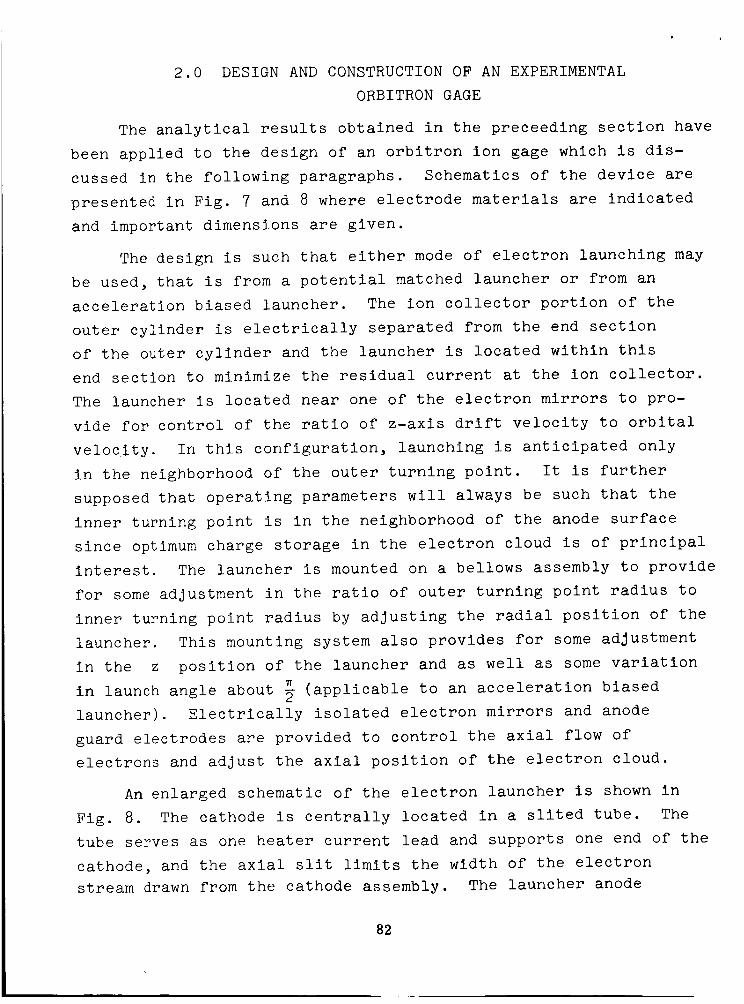
2.0 DESIGN AND CONSTRUCTIONOF AN EXPERIMENTALORBITRON GAGE
The analytical results obtained in the preceeding section have
been applied to the design of an orbitron ion gage which is dis-cussed in the following paragraphs. Schematics of the device are
presented in Fig. 7 and 8 where electrode materials are indicated
and important dimensions are given.
The design is such that either mode of electron launching may
be used, that is from a potential matched launcher or from anacceleration biased launcher. The ion collector portion of the
outer cylinder is electrically separated from the end section
of the outer cylinder and the launcher is located within thisend section to minimize the residual current at the ion collector.
The launcher is located near one of the electron mirrors to pro-
vide for control of the ratio of z-axis drift velocity to orbital
velocity. In this configuration, launching is anticipated only
in the neighborhood of the outer turning point. It is further
supposed that operating parameters will always be such that the
inner turning point is in the neighborhood of the anode surface
since optimum charge storage in the electron cloud is of principalinterest. The launcher is mounted on a bellows assembly to provide
for some adjustment in the ratio of outer turning point radius to
inner turning point radius by adjusting the radial position of thelauncher. This mounting system also provides for some adjustment
in the z position of the launcher and as well as some variation
in launch angle about _ (applicable to an acceleration biasedlauncher). Electrically isolated electron mirrors and anode
guard electrodes are provided to control the axial flow ofelectrons and adjust the axial position of the electron cloud.
An enlarged schematic of the electron launcher is shown in
Fig. 8. The cathode is centrally located in a slited tube. Thetube serves as one heater current lead and supports one end of the
cathode, and the axial slit limits the width of the electronstream drawn from the cathode assembly. The launcher anode
82

E-i
.,--I
©.i.a
0
E-I
of
'-'I
Ol
.J._l
J
®
0
o%
,--IM
"1
I"M
-,qi
•_ cd
E_ c_)_ o
I,.q
I
!I
i
A A A lk
'1 | i||
I|
f
®
r--t0
01"-4
°l
IOd
I U
I o
_t
I
\
n
0
k_
Od
il
2
1
Ol1-141
4--_1
Ol
(DI
Ol,---it
OI
,,.-_ r
_L
4--_1
Ol
C'?l
0) 1
Ol
0
4-_
©
0
r./?
_0
o
0
,--4
(D
_D
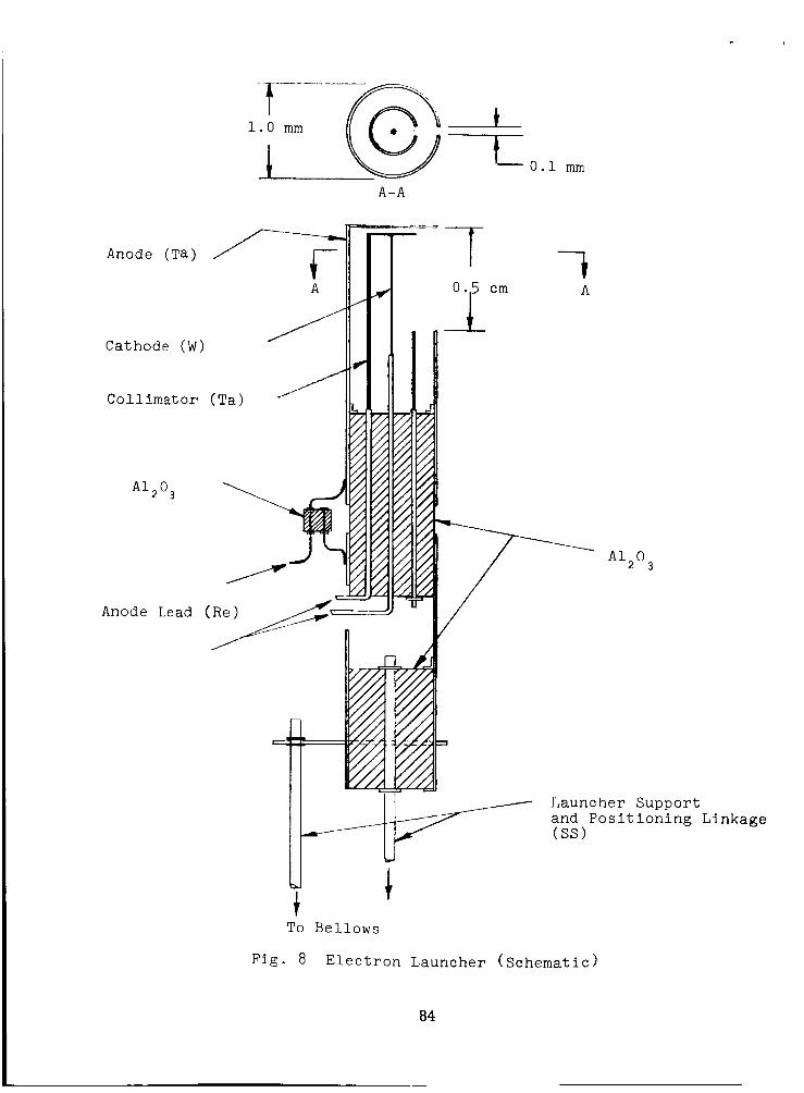
}1.0 mm
A-A
mm
AnodeITa)//_----_
Cathode (W) ///
Collimator (Ta) //
AI203
Anode Lead
Fig. 8
AI203
Launcher Support
and Positioning Linkage
(SS)
Electron Launcher (Schematic)
84

surrounds the cathode assembly and has an axial slit which is
aligned with the cathode assembly slit. This slit system results
in the ejection of a narrow stream of electrons from the launcher.
The center plane of the sllt system is oriented at an angle of
with respect to the radius vector of the orbitron. In the
potential matched mode of launching the launcher anode is biased
to match the local space charge dependent potential and the
cathode assembly is biased below the anode such that the potential
difference between them corresonds to the desired electron ejection
..... o_ ............ _ _,,_ _±,_uic energy.......... ±_le electron
launch rate is controlled by variation of the heater current only.
In the acceleration biased launching mode, the launcher anode is
biased below the local space charge dependent potential such that
the potential difference corresponds to the desired electron
kinetic energy in the neighborhood of the outer turning point.
However, to minimize space charge limitations within the launcher
and to assist in collimating the ejected electron stream the
launcher cathode assembly should be biased somewhat below the
launcher anode. Thus the electrons leave the anode sl_t _n a
well defined direction and with a few eV of kinetic energy.
All electrodes are mounted on support rods which pass through
ceramic insulators located on a single flange thus making the
entire assembly demountable.
With the above geometrical configuration and for anode
potentials between 250 and i000 volts corresponding to the mean
electron kinetic energy range from about 75 to 300 eV, the orbi-
tron ion gage performance may be experimentally studied and
evaluated over the sensitivity range from about 103 to 105 Torr -I.
85

APPENDIXA
Stability Analysis
If an electron is in a stable orbit, any small perturbation of its
radial motion, resulting in an incremental displacement from its orblt_must be resisted by a force which tends to restore the electron motion to
its original orbit. Thus, the incremental restoring force resulting froman incremental displacement of the electron from its orbit must have the
following form if the orbit is to be stable
df =-k dr, (AI)
where k is a positive constant. Taking the differential of both sides
of Eq.(21) gives
d(mr) _ df.: - ÷ e _ (A2)
For these two equations to be identical in form, it is necessary that
3_---_2+ e d E(r) > 0, (A3)mr4 dr
for all points along the trajectory.
The least stable point in an ellipse-like trajectory is the outer
turning point, where the electron is most distant from the force center,
thus experiencing the smallest electric force, and also where the gradient
of this force is smallest. Thus, a stability criteria which assures that
the electron trajectory is stable at the outer turning point is sufficientto assure that the entire orbit is stable.
The outer turning point of an electron in an undisturbed orbit coin-
cides with the outer boundary of the space charge cloud, the boundarybetween regions 2 and 3. However, if the electron trajectory has been
perturbed such that the actual trajectory has been displaced radially by
a positive increment from the original trajectory, its outer turning point
will occur in region 3, beyond the space-charge boundary. Therefore, the
field derivative appearing in Eq.(A3) must be evaluated ir_nediately outside
A-I
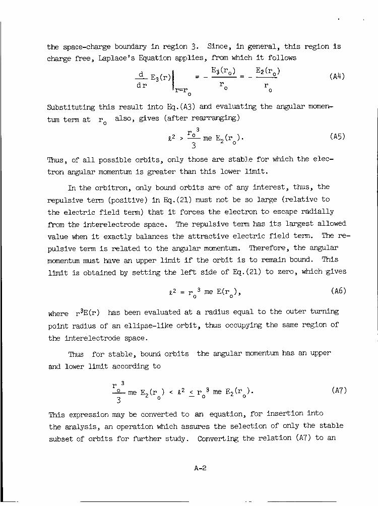
the space-charge boundary in region 3. Since, in general, this region ischarge free, Laplace' s Equation applies, from which it follows
d E3(r)l - E3(r°)--- E_(r°) (A4)
dr I r rr:r o oo
Substituting this result into Eq. (A3) and evaluating the angular momen-
tum term at ro also, gives (after rearranging)
Z2 > r°-_3me E2(r ). (A5)3 o
Thus, of all possible orbits, only those are stable for which the elec-
tron angular momentum is greater than this lower limit.
In the orbitron, only bound orbits are of any interest, thus, the
repulsive term (positive) in Eq. (21) must not be so large (relative to
the electric field term) that it forces the electron to escape radially
from the interelectrode space. The repulsive term has its largest allowed
value when it exactly balances the attractive electric field term. The re-
pulsive term is related to the angular momentum. Therefore, the angular
momentum must have an upper limit if the orbit is to remain bound. This
limit is obtained by setting the left side of Eq. (21) to zero, which gives
Z2 = ro3 me E(ro) , (A6)
where r3E(r) has been evaluated at a radius equal to the outer turning
point radius of an ellipse-like orbit, thus occupying the same region of
the interelectrode space.
Thus for stable, bound orbits the angular momentum has an upper
and lower limit according to
3r
o me E2(r ) < £2 < r 3 me E2(ro). (A7)3 O -- O
This expression may be converted to an equation, for insertion into
the analysis, an operation which assures the selection of only the stable
subset of orbits for further study. Converting the relation (A7) to an
A-2

Thus the effect of the perturbation, independent of the form of the per-
turbation interaction, is that the electron oscillates about its original
trajectory at the frequency given by Eq.(AI4) and with the amplitude given
by Eq. (AI6). The oscillation will continue for avery long time since the
only damping in the system is radiation damping of the electron which has
been neglected in Eq. (AI3) since it is extremely small. The energy ra-_i 0
diated during one orbit is typically of the order of i0 T(r i) to 10-15
T(r. ) where T(r i) is the kinetic energy of the electron at the inner turn-iing point (maximumkinetic energy). Since the system is nonlinear _ is
not a constant. In fact, _ increases as r decreases (as the electron2_
proceeds along its trajectory from r ° ). The oscillatory period, -_-, isof the sameorder of magnitude as the orbit period. Thus, the oscillatory
electron response actually distorts the entire orbit.
For k<0 in Eq.(AI0), the response of the electron to a perturbationis essentially different from the above results. The solution to Eq.(AI3)
is then
×(t) = Xo cosh _t + X___osinh _t, (A18)
where(i-3a2) E2(ro) 2 1
mr "_ <_"
o
2 1Thus, for _ <5' a perturbation which produces either a displacement
from the original trajectory or an increment in the radial velocity (or
both), no matter how small, yields an electron response which diverges
from the original trajectory without limit.
(AI9)
A-5

wherek (3_2-I) e E2(r o)
_2 _ - (A14)m mr
o
The solution to this equation describes the electron response to the per-
turbation. Since the form of the perturbation forcing function is un-
known, the most general method of proceeding with the solution to Eq. (AI3)
is to assume that at the end of the perturbation, the electron has been
i., 2 (thedisplaced by ×o and given a velocity increment _o' where _m×o
increase in radial mode kinetic energy) is assumed small compared to
Z2. Taking the end of the perturbation as the zero-time reference,
2mr 2o
the parameters ×o and Xo become the initial conditions necessary to
specify the integration constants in the solution of Eq.(AI3).
For k>0, the solution to Eq.(AI3) is
x(t) = Xo cos _t + X-_°sin_ _t. (AI5)
For k>0, from Eq.(Al4) it is obvious that _ decreases as _ de-
creases. Therefore, the amplitude of the electron response in Eq.(AI5)
increases as _ decreases and the frequency of the oscillatory response
decreases as _ decreases. The maximum displacement of the electron
from its original trajectory is, from Eq.(AI5),
[ ]½Xmax= XO l+--Xo2CO2
(AI6)
Using Eqs. (A8) and (AI4), this may be rewritten in terms of the kinetic
energy given to the electron during the perturbation AT, and the original
electron kinetic energy at the outer turning point T(ro),
(Xma.x] 2 Xo 2 a 2 AT
,_ ) = r--,z + ---- • (AIT)o (3 e2-1) T(r )o
A-_

Thus the effect of the perturbation, independent of the form of the per-
turbation interaction, is that the electron oscillates about its original
trajectory at the frequency given by Eq. (AI4) and with the amplitude given
by Eq. (AI6). The oscillation will continue for avery long time since the
only damping in the system is radiation damping of the electron which has
been neglected in Eq. (AI3) since it is extremely small. The energy ra-
0 10_15diated during one orbit is typically of the order of lO-I T(r i) to
T(r ) where T(r i) is the kinetic energy of the electron at the inner turn-i
ing point (maximum kinetic energy). Since the system is nonlinear m is
not a constant. In fact, _ increases as r decreases (as the electron2_
proceeds along its trajectory from r° ). The oscillatory period, -_-, is
of the same order of magnitude as the orbit period. Thus, the oscillatory
electron response actually distorts the entire orbit.
For k<0 in Eq.(AI0), the response of the electron to a perturbation
is essentially different from the above results. The solution to Eq.(AI3)
is then
x(t) = Xo cosh _t + X_p_osinh _t, (AI8)
where
(I-3_2) E2(ro) _2<_._02 = ,.
0
2 1
Thus, for a <7' a perturbation which produces either a displacement
from the original trajectory or an increment in the radial velocity (or
both), no matter how small, yields an electron response which diverges
from the original trajectory without limit.
(Ai9)
A-5

APPENDIXB
Effective Eccentricity
Thetrajectory of a bound particle in a r -2 central force field isin general a closed ellipse (4) (provided wave effects and relativistic ef-
fects are negligable). The radial position of the particle as a function
of the azimuth angle 0 is given by
1 (BI)r --
which is the standard form in polar coordinates of the ellipse sketch
below,
_nd where
t-r. r __
1 o
-- 2a
k _ force constant,
_ particle angular momentum,
m _ particle mass,
ro_ outer turning point,
rim inner turning point,^
r _ semi-latus rectum of the ellipse.
t2 b
A-6

The radial component of the particle acceleration is given by
£2 k=
m2r 3 mr 2(B2)
The radius at which the particle radial acceleration passes through zero,.
is obtained from this equation by setting r = 0 and solving for r
r(r=0) : r _2= -- • (B3)km
Substituting this value for
gives
^
r into Eq.(BI) and solving for
^ ]ie = + n -,(n odd). (B4)
-- 2
Thus, the polar coordinates of the particle at the instant that the radial
acceleration passes through zero are just the coordinates of the end points
of the semi-latus recturn of the ellipse.
In terms of standard elliptical parameters, the radius to the outer
turning point is given by
r° a(l+e c) , (B5)
_nd the !e.n4_thof the sem_-!atus rect_n is given by
b2r : _- , (B6)
and the ellipse eccentricity e must satisfy the relationc
b 2 = a2(l-ec2), (BT)
where 2 a e major axis of the ellipse,
2 b e minor axis of the ellipse.
Eliminating a and b in Eq.(B5) through (B7) gives
^
r _ l-e • (B8)r c
o
That is, the ratio of the radius at which the radial acceleration
is zero to the outer turning point radius is a function only of the eccen-
tricity of the ellipse. In retrospect, this may be demonstrated more
A-7
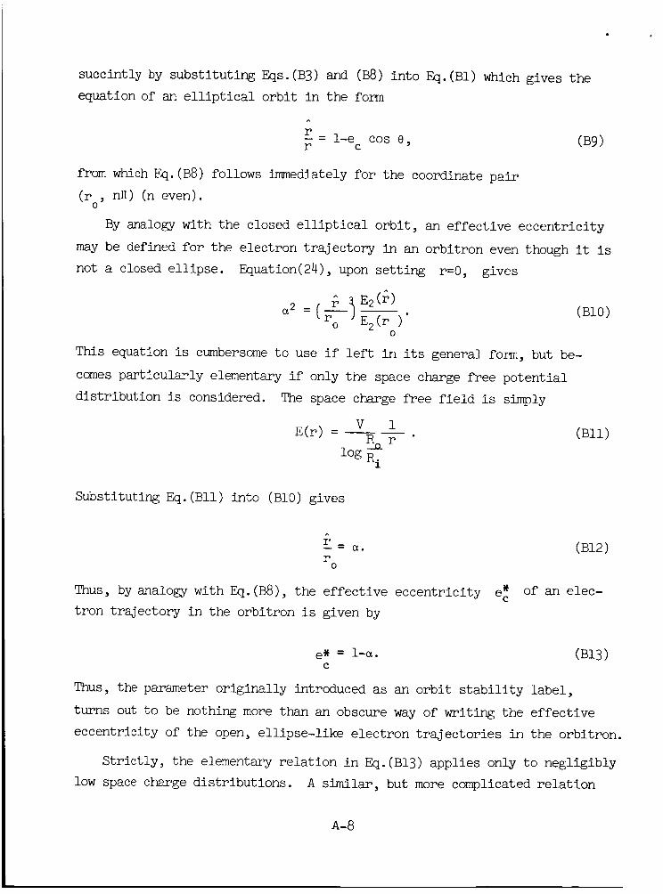
succintly by substituting Eqs.(B3) and (B8) into Eq.(BI) which gives theequation of an elliptical orbit in the fonn
^
r
--= l-e cos 8, (Bg)r c
from whichEq.(B8) follows immediately for the coordinate pair
(r , nH) (n even).o
By analogy with the closed elliptical orbit, an effective eccentricity
may be defined for the electron trajectory in an orbitron even though it is
not a closed ellipse. Equation(24), upon setting r=0, gives
E2 (_)
o
This equation is cumbersome to use if left in its general form, but be-
comes particularly elementary if only the space charge free potential
distribution is considered. The space charge free field is simply
E(r) - V 1 . (BII)Ror
log Ri
Substituting Eq.(BII) into (BI0) gives
m
-- (BI2)ro
Thus, by analogy with Eq.(B8), the effective eccentricity
tron trajectory in the orbitron is given by
* of an elec-ec
e* = l-a. (BI3)c
Thus, the parameter originally introduced as an orbit stability label,
turns out to be nothing more than an obscure way of writing the effective
eccentricity of the open, ellipse-like electron trajectories in the orbitron.
Strictly, the elementary relation in Eq.(BI3) applies only to negligibly
low space charge distributions. A similar, but more complicated relation
A-8

may be derived for non-negligible space charge distributions. However,
the essential conclusion is (and applies to any space-charge distribution)
that _ is simply a measure of the effective eccentricity of the ellipse-
like electron trajectories.
A-9
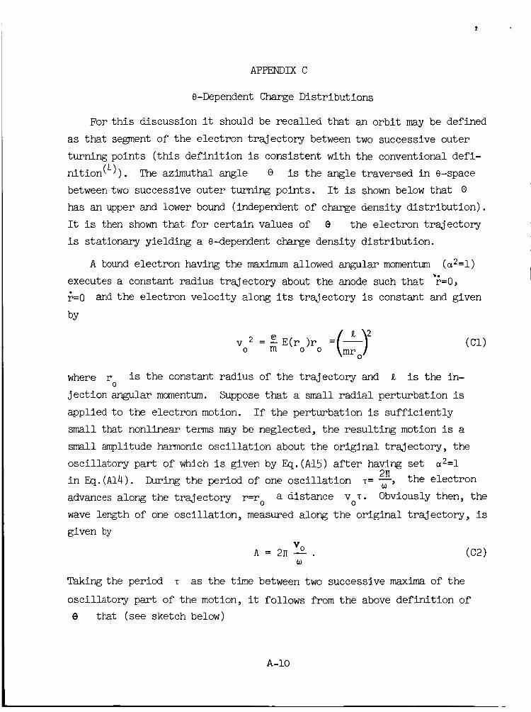
APPENDIXC
8-Dependent Charge Distributions
For this discussion it should be recalled that an orbit maybe defined
as that se_Fnentof the electron trajectory between two successive outer
turning points (this definition is consistent with the conventional defi-nition(4)). The azimuthal angle 0 is the angle traversed in e-space
betweentwo successive outer turning points. It is shownbelow that 0
has an upper and lower bound (independent of charge density distribution)•
It is then shownthat for certain values of 0 the electron trajectory
is stationary yielding a e-dependent charge density distribution.
A boundelectron having the maximumallowed angular momentum (_2:1)%,
executes a constant radius trajectory about the anode such that r=0,
r=0 and the electron velocity along its trajectory is constant and given
by
v 2 =eE(ro m o)ro =( _m-_o_-(el)
where r is the constant radius of the trajectory and £ is the in-o
Jectionmng_larmomentum. Suppose that a small radial perturbation is
applied to the electron motion. If the perturbation is sufficiently
small that nonlinear terms may be neglected, the resulting motion is a
small amplitude harmonic oscillation about the original trajectory, the
oscillatory part of which is given by Eq.(Al5) after having set _2=I2H
in Eq.(Al4) During the period of one oscillation _= --, the electron•
advances along the trajectory r=r o a distance VoT. Obviously then, the
wave length of one oscillation, measured along the original trajectory, is
V o
A = 2n _ . (C2)
given by
Taking the period T as the time between two successive maxima of the
oscillatory part of the motion, it follows from the above definition of
8 that (see sketch below)
A-IO

A=r @0
(c3)
since the average value of the oscillatory amplitude is zero as may be
seen from
= r + 1 _T x(t)dt : ro T 0
0
upon substituting from Eq.(AI5) for ×(t).
(C4)
Eliminating A between Eq.(C2) and (C3), substituting from Eq.(Cl) for
and substituting from Eq.(Al4) for _ (with a2=l), givesVo_
e : n. (c5)M
The subscript M (for maximum) has been applied to e since this
value was obtained for the maximum angular momentum and as the angular
momentum decreases e must decrease. An important observation is
that the result in Eq.(C5) is independent of electric field distribution
and therefore of the charge density distribution.
A-II

The minimum angle traversed in one orbit is that associated with an
g=0 trajectory (which of course violates t_e stability criteria and pre-
sents obvious practical difficulties). However• if practicable and if
allowed• an _=0 electron would pass through the origin (r=0) and proceed
to r=r on the opposite side of the anode. The angle between two succes-o
sive outer turning points is H and therefore
e = _ (C6)m •
where the subscript m _or minimum ) has been applied since an angle smaller
than this value would have no physical meaning.
From the above discussion, it follows i_nediately that all electron
trajectories in an ortitron must satisfy
< 0 < _-_. (C7)
Since the derivation of these limits did not involve the form of the elec-
tric field distribution• Eq. (C7) is applicable to any charge density dis-
tribution provided only that the charge is uniformly distributed in e-space.
It is i_nediately obvious that the _=0 trajectory results in a non-
uniform e-distribution of the space charge, since on a time average the
charge is mostly in the neighborhood of the turning points where _=0.
The _=0 trajectory thus yields two charge clusters, each in the neighbor-
hood of r=r o but one at e=e and the other at e=e + n. Thus for allo 0
e not near e or e +_, p =0. An important observation concerning thiso o
charge distribution is that it is stationary in e-space. As the number
of _=0 electrons are increased, the charge density approaches saturation
in only two regions while in the remainder of the interelectrode space the
charge density is zero. Such trajectories then make very inefficient use of
the interelectrode space and the applied potential.
A sequence of possible trajectories exists having $>0 which like the
_0 trajectory, tend to produce localized stationary charge clusters.
The trajectories belonging to this series are those for which the angle be-
tween successive outer turning points satisfies the relation
A-12

nO= 2m_(n>m), (C8)
where n and m are positive integers containing no commonfactor
(and of course e must satisfy Eq.(C7).) The n=2, m:l trajectory has
already been discussed (_:0). The n:3, m:2 and the n:5, m--3 trajec-tories are sketched below.
n=3m=2
The-important property of this series of trajectories is that after n
orbits (or m circuits of the anode) each closes on itself and repeats
indefinitely. Thus, the n-orbit trajectory considered integrally is station-
ary. The n-orbit closed trajectory produces 2n stationary charge clusters
in the neighborhoods of the 2n turning points of the integral, closed
trajectory. All the members of this series of trajectories make more or less
inefficient use of the interelectrode space, approaching saturation in a dis-
crete set of small regions. The maximum charge that can be stored in the inter-
electrode space under these conditions is substantially less than that cor-
responding to a uniform approach to saturation over all e-space. As n be-
comes large, the charge clusters begin to overlap and the charge distribution
in e-space begins to smooth, eventually becoming approximately uniform.
From the above discussion, it is clear that the n-orbit closed trajectories,
in which n is small, should be avoided in the orbitron. This may be
A-13

accomplished by disallowing those values of _ within the stability range
which correspond to stationary, closed trajectories. It turns out that the
specification of this discrete set of o's involves considerable numerical
computation and a complete solution to the electron motion in the space
charge dependent potential distribution.
For all trajectories which do not satisfy Eq. (C8), e is an irrational
multiple of 2n, the trajectories never close, the orbits continue to pre-
cess, and the charge density is uniform in e-space.
A-14

APPENDIXD
Interpretation of 8
The electric field distribution in Region 3, outside the space chargecloud, is obtained from Eq. (15) by taking the negative derivative with
respect to r. Applying Eqs.(54) and (55) and evaluating at R givesothe electric field at the outer boundary
r
E3(Ro) = {V+l,(re)log _.o _ l(ro)} I i• _ " 5--
-'i 10g _-_ _oRi
(DI)
The space charge free electric field at the outer boundary is obtained
from this same equation by setting all the charge integrals to zero
Ecf(Ro ) = _ V . ___ilog Rn Ro
R.1
(D2)
The change in electric field at the outer boundary resulting from the
charge insertion is
r o
Ecf(Ro)-E3(Ro) = +{-I'(ro)log _+ I(ro)}
i i
R R 'log -9-o o
Ri
The fractional change in electric field, relative to the final value, is
Ecf(Ro)-E3(R o)
E (Ro)3
r o
-I' (ro)log _ + l(ro)
V+I, (ro)log ro _ I(ro)
Substituting from Eq.(61) for l'(r o) gives
(D3)
(D4)
Ecf (Ro)-E3(Ro) _ Ecf(Ro)
ES(Ro) - E3(Ro)
[u2eV Ro i
_ 7 -log Ro(D5)
A-15

Therefore by comparison with Eq.(65), it follows that
• R
E<f(R°) - i} log __o.R.l
(D6)
From this equation it is obvious that B is positive for all nonzero
charge densities and approaches zero as the charge density approaches
zero. .8 is essentially a measure of the fractional reduction in elec-
tric field at the outer boundary relative to its final value after charge
insertion.
An informative alternate form of Eq.(D6) is
E3(R o) =
from which it follows that
V
Ro(8 + log ____oo)(D7)
Lim E3(R o) = O. (D8)
Thus, the electric field at the outer boundary is always greater
than zero for acceptable values of 8.
A-16

9 •
APPENDIX E
Charge Optimization ,
It follows immediately from Eqs.(16), (52), (53) and
(54) that
--I' (r o) = -- _ p (r)r dr _ eNL r°/ d____r eNL .
ri _o _Eo r i _ : 2_o
(El)
Therefore Eq.(61) may be written
Ro]2T(ro) log R--_eN L = 2,._oV - _2 eV (E2)
ro •R i
Since
r ° rr° - log + log i
logRi _ _ , (E3
Eq.(E2) may be written
2T(r o) log R_lllLI e2 eV
eN L = 2_coV - _.ri ro l(ro)
log_ + log_- _(-go_JThe left side of this equation is the total charge stored in
unit length of the rotating electron cloud. Optimizing N L
involves several operations: Maximizing NL with respect to
ri; maximizing N L with respect to _2 but consistent with
the other requirements that _2 must satisfy; and determining
the behavior of NL as a function of other prescribed param-
eters such that values are prescribed which tend to optimize NL.
(E4)
A-17

P
Maximizing N L with respect to r i involves minimizing
the denominator of Eq.(E4) with respect to r i. Although the
ratio r-_° is fixed by prescribing _2 and B, either ro orrl
r i may be prescribed independently. Full advantage may be
taken of this degree of freedom by prescribing that
r i = R i + 8, (E5)
such that
6- << I. (E6)
R i ri
This prescription is equivalent to locating the inner turning
point immediately outside the anode surface such that the elec-
trons pass by the anode at a distance Just sufficient to assure
that they do not collide with the anode surface. Under this
condition _ may frequently be neglected in the analysis
(for _2 not close to 1). This simplifies the denominator
of Eq.(E4) and removes any explicit dependence on R i since
the first term may be written
ri - 8-_-)=log (i+ 6 ) = 8 << 1 . (E7)log Ri log (i+ Ri r-_ r i
This operation maximizes NL with respect to r i while
leaving the ratio r°m unchanged and without substantially
rl I(ro)affecting the value of
I'(r o )
Maximizing NL with respect to e2 is not so elementary.
A plausibility argument may be constructed, based on an approx-
imation to I(rn) obtained by using the radial component ofI'(r o )
A-18

the electron velocoty applicable to negligibly low charge den-sities• Although this approximation does not contain some of
the important parameters (for example 8 ), it must indicate
correctly at least the direction of the variation in NL asa function of _2 . That is, the result must correctly indi-
cate, even for non-negligible Charge densities, whether N L
is an increasing or decreasing function of _2 (it turns out
this is the only information required to maximize N L with
respect to e2). This conclusion follows from the fact that
p(r) has the same general shape for any value of N L. The
principal influence of NL upon p(r) is that variations in
N L raise or lower p(r) and only secondarily increase or de-
crease the distance between turning points (space charge
50undaries). The shape of p(r) is principally determined by
the form of the function (which is generally similar for any
N_ and _2. The first integral of the charge density is in-
dependent of the shape of p(r) The ratio I(ro) is inde-• l,(ro)
pendent (exp!ic _+_'' _T_a) of and is principally a function of_m
the shape of the charge density distribution. Therefore, con-
clusions based on the shape of one charge density distribution
must be generally applicable to other similar charge density
distributions since their shapes do notdiffer substantially.
The derivation of the analytical expressions necessary to
I(ro) depends on _2 isexpose the way that the ratio i,(ro)
connected intimately with the trajectory analysis in Appendix F,
which is therefore used freely in the following analysis.
Equation (F13) may be used to obtain an approximate value
for the charge integrals I'(r o) and I(ro). Substituting
Eq.(F13) into Eq.(52), substituting the result into Eq.(16)
and applying Eqs.(54) and (F16) gives
A-19

x
eNL i _ d xl'(r) = -- -_-
2_e o [2ax- x2]½o
=-eN L . I cos-l(1-%),2_- ° ._
where a is defined by Eq.(FI4). Evaluating this equation at
r , (x = 2a), gives the expected resulto
e N L
l,(ro) = 2_Eo '
(E8)
(E9)
which is the same for all charge density distributions since
l'(r o) is independent of the shape of p (r).
Substituting Eq.(ES) into Eq.(17), performing the co-
dr and applyingordinate transformation of Eq.(F3) on _-
Eq.(55) gives
I(r) =eNL i x__ x dx
2_Eo _ f cos -I(I-[)o
(EIO)
where y is defined in Eq.(F4) or (FI2). It is convenient to
make a new coordinate transformation such that
= cos -l(l- _) ,(Ell)
with the limits
x = 0 , _ = 0
X = X _ =0 _
(El2)
Equation (El0) may then be written
A -20

• t
eNL b _ _ sin _ d_l(r) - 2_o . -_--
o i - b' cos_(El3)
where
i _2 _ 2).
2_2_ y2
Integrating Eq.(E13) by parts gives
(El4)
l(r)- eNL {7--_log (l-b cos _)-- 71 flog (l-b cos_)d_}. (El5)O
2_E0
Since b << 1 (the leading term in its expansion as a function
Aof A is _) (see Eqs.(F8) and (FI2)), the logarithms in Eq.(E15)
may be expanded in powers of (b cos _ ). Second order and higher
terms may be neglected for the present purpose. After perform-
ing these operations• Eq.(E15) becomes
eNL k (sin _ -_ cos _). (El6)l(r)_ 2_%
Evaluating this expression at _,(_ = _), gives
eN Ll(r ) - b . (El7)
o 2_e o
From Eqs.(E9) and (El7)
I(ro) = b •
I'(r ° )
(El8)
A-21

and from Eq.(EI4)
l(ro) I (_l,(roY = _ _ 2) ,
(El9)
and applying Eq.(FI2) gives
(for
l(ro) I [l--e2] a
-
Therefore the denominator of Eq.(E4) may be written
a 2 near i)
(E20)
rolog + log rl
I(ro) r___o_ A
_--_ _ log rl _ ;
(E2I)
and from Eqs.(F4) and (FI2) it follows that
r__£_
log ri
from which Eq.(E21) becomes
A; (E22)
rlog ri + log o _ = _+
R i rl rl
6 1 2
=r-_2(z-_ ).
Therefore, under the condition expressed in Eq.(E5) and for
near I, the limiting value of the total charge stored in unit
length of the rotating electron cloud is
Llm eNL= 2_%V_6
a2 ÷ i
2T(ro)log Ro ]eV R?i "
(E23)
a 2
(E24)
A-22

RoUsing Eq. (65) to eliminate log R--i , which in this dis-
cussion is an unimportant parameter, Eq,(E24) may be written
in the alternate form
4_° 8T(r°) rl (E25)Lim NL =
_2 ÷ 1 e 2 6
from which it is obvious that NL increases with increasing
r i and decreases with increasing 6. This limiting charge
corresponds to a thin, high density charge sheet immediately
outside the anode surface, the electrons of which execute cir-
cular trajectories.
_2=i leads to serious practical difficulties since the
electron launcher cannot be made infinitesimally small. Long
electron life times can be achieved only if the electron tra-
jectory is sufficiently eccentric that the electrons miss the
launcher during the first few passes after injection (it is
assumed that after the first few passes, the electron has drifted
far enough along the z-axis to miss the launcher altogether).
Therefore, optimization of N L is not a simple maximization
operation. The optimum N L is that associated with the largest
a2 for which the trajectory is sufficiently eccentric that the
probability of collision with the launcher during the first few
orbits is negligibly small. It is only under this condition
that the charge density can be pumped up to its equilibrium value
all along the z-axis and a uniform charge density cahieved in
z-space (if the electrons returned to the launcher at the end of
the first circuit of the anode, all the charge would be concen-
trated in the z-neighborhood of the launcher).
Concerning the remaining parameters in Eq.(E4), it is ob-
vious that NL increases with V and increases with decreasingRo
A-23

APPENDIX F
Trajectory Analysis for Low Charge Density (Approximate)
If the total charge stored in the rotating electron cloud
is sufficiently low that the space charge dependent potentialdistribution does not differ substantially from the space charge
free potential distribution, and if the electrons are injectedinto trajectories which are not very eccentric, then Eq.(26) may
be approximated by an integrable function. The results obtainedare not strictly applicable to the more interesting and useful
high density, moderate eccentricity space charge configuration,however the results provide considerable insight into the low
density electron dynamicsand may be used to clarify and assistthe correct interpretation of other results which are directly
applicable to moderate eccentricity, high density space charge
distributions.
Under the above restrictions, the radial component of the
electron velocity is given by
i
r 2 r 2 '
where
2 eV= . (F2)Ro
m log R-T
For mathematical convenience, let
r-- = y + X ,ro
(F3)
A -21_

• a
where r i
Y - r (F4)o
The trajectory turning points then occur at
and
r = r i , x = x i = 0 , (inner turning point) ,
r = r , x = x = l-y,(outer turning point) .O o
(F5)
(F6)
Recalling that the trajectories considered in this Appendix are
not very eccentric, y is near i and for even the maximum
value of x,
x << i (F7)o
Similarly, _2 is not much less than i and may be written
= z - A , (F8)
where
0 < A << i _F9)
From Eqs.(Fl) and (F4), it follows that
_2 --_2log ! + (I ) = O. (FlO)y 2 y
The logarithmic term in this equation may be approximated by
the first two terms of the well known Taylor expansion in the
neighborhood of i,
I 2=. =( y1 -- i_I]___(i___] • (FII)log
A-25

t
Substituting Eq. CFII) into Eq. GFI0) and solving the resulting
quadratic equation for y gives
= l+m 2 2-A- ~ l-A = _2 (FI2)
Y 3__2 2+A
a result which is needed frequently later on.
Using Eq.(F3) to eliminate r in Eq.(FI) and performing
an expansion similar to Eq.(Fll) and taking account of Eq.(F10)
yields an approximate analytical expression for the radial com-
ponent of the electron velocity
i i i
= K-22 t[3012--Y 2) 2 [2ax-x (FI3)2Y
where
c_2-Y 2 A
)=_. (FI4)
The solution to this differential equation gives the electron
radial position as a function of time. Taking the zero time
reference to correspond to the inner turning point of the elec-
tron trajectory and integrating Eq.(F13) gives
1 x
,o 22yoSdxii _3a2 ._2 [2ax_x2]_
1
y~ r cos (i-).
K7 3a2-y 2
(FI5).
A-26

From this equation, the orbit half-period
immediately by setting r=r ° (x=_),
T ! is found
3a2--y 2(FI6)
Using this result, Eq.(FI5) may be written
X = X sin 2 _to 2_' '
and transforming from x-space back to r-space, the radial
position of the electron as a function of time is given by
(FIT)
_ : _tr 1 -- (l--y) cos2_,ro
The position of the electron in e-space may be obtained
as a function of time by substituting Eq.(FI8) into Eq.(20)
and integrating (again taking the zero- e reference to cor-
respond to the inner turning po{nt),
t
o
_td (Ti-)
[1-( ) cos Tv]
where _'
velocity at the outer turning point and is given by
is again the half-period and _ is the angularO
1
= 2T(roO2)]_o [ m
(FI8)
(FIg)
(F20)
A-27
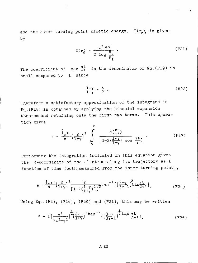
and the outer turning point kinetic energy,by
T(ro) , is given
e2 eV
2 log RoRi
The coefficient of
small compared to
_tCOS _-y
1 since
in the denominator of Eq.(FI9) is
(F21)
Therefore a satisfactory approximation of the integrand in
Eq.(FI9) is obtained by applying the binomial expansion
theorem and retaining only the first two terms. This opera-
tion gives
t
•e = -_--(y_V] [1-2( ) cos _t]O m
(F22)
(F23)
Performing the integration indicated in this equation gives
the 8-coordlnate of the electron along its trajectory as a
function of time (both measured from the inner turning point),
e__q3_( 2 ]2 2 i 3 _ t
- an- {(_y--_-l]tan_'}e = , _l-_y_ [i_4(_)219t
Using Eqs.(F2), (FI6), (F20) and (F21), this may be written
] ]2tan-1{(3--y_)2tan 2--_'_t}
(F24)
(F25)
A-28

where the approximation has been made
[l-4[!=!_}l+_)] --1
because of Eq.(F22). Setting t=_' in this equation gives
the azimuthal half-angle of the electron trajectory
ict2 2 _ 2
Using this result, Eq.(F25) may be written in the alternate
form
e 2e'tan -l 3-_ ]_tan _t= T { (3-T_-_' 2_,}.
(F26)
(F27)
(F28)
Using Eq.(FI2), y may be eliminated from Eq.(F27) in favor of
_2 which gives
. 2c_2 '_2
e,= _ %[_J (F29)(3_a2)'
from which it follows that
Lime' =
_2 _ 1
(F30)
a result which was derived from other considerations in
Appendix C.
A-29

Considering Eqs.(F18) and (F25) as a set of parametricequations in t, r may be expressed as a function of e
by eliminating t. The result of this operation (after usingEq.(F12) to eliminate y) is
r_rl 3a2_l]tan2 Fl+a 2 2 2ro--r--(3-a2 {<2_---_T-](3-a2) _}. (F31)
An immediate application of this equation is to compute
the values of a 2 for which the electron trajectories are
closed and stationary so that these a's may be rejected in
prescribing the launch parameters. From Appendix C, the first
non-degenerate stationary trajectory has m=3, m=2. Therefore2_
at r=ro, e=_-. Substituting these values into Eq.(F31) gives
[l+a212(3-a2)_ - _ (n=3 m=2) ;_2e 2 _ 3 2 " "
(F32)
from which it follows that
a 2 = 0.95 , (n=3, m=2). (F33)
Similarly, the second closed, stationary trajectory occurs for
a 2 = 0.93 , (n=5, m=3). (F34)
The separation in a-space between successive stationary
trajectories decreases as n increases. This implies that
either the launch parameters must be controlled very precisely
or a 2 must be sufficiently small that n is large and the
charge clusters in the neighborhood of the 2n turning points
A-30

overlap sufficiently to yield an approximately uniform charge
density distribution in e-space.
A-51

PART II MAGNETRON GAUGE
i.i INTRODUCTION
In the initial description of the magnetron gauge using
auxiliary cathodes, Redhead (6) showed that the gauge could
be used to l0 -12 Torr but that it was non-linear below about
5 x l0 -10 Tort. Later work (7)'(8), using different calibration
techniques and extending the measured low pressure limit to
3 x l0 -13 Torr, confirmed Redhead's work. However, in total,
very little work has been carried out at pressures below
i0 -I0 Tort where the aim has been to characterize the per-
formance of the magnetron gauge over the range of the many
variables which exist. For instance, in his original paper,
Redhead _6#"" used an anode voltage of 6000 v and a magnetic
field of 1000 gauss in measuring the variation of the cathode
current with pressure. Similarly, later work (9) has tended
to use similar values for the anode voltage and magnetic
field. However, work at the National Research Corporation _10)"
has shown that below l0 -10 Torr, the sensitivity (S = i+/P)
of the normal magnetron goes through a maximum as the anode(il)
voltage is varied from i000 to 7000 volts. More recently
Redhead has investigated changes in both anode voltage and
magnetic field over a range of pressures extending down to
1.3 x l0 -ll Tort. This work has shown that the magnetron
dlschargeexlsts in two states which may be characterized
by the nature of the radio frequency oscillations exhibited
by the gauge. In the pressure range 1 x l0 -10 Torr to
l0 -6 Torr and at low magnetic fields (State I), the low
frequency noise was large and stable r-f oscillations were
not observed. At higher magnetic fields (State II), stable
oscillations of very narrow band width were observed in the
frequency range 15 - 100 Mc/s. (When used as a pressure
gauge, the magnetron is operated under the conditions
corresponding to State I.) In addition, Redhead reported
86

that oscillations were not observed below l0 -10 Torr and it
appeared that two separate states did not exist at these
pressures. These results suggested that the change in
oscillatory behavior may be closely related to the transition
from linear to nonlinear operation at approximately 2 x l0 -10
Tort. They also suggested that the oscillations might
provide an indication as to whether or not a gauge was
^_o_o+4_ under linear _,,__o._v_- ...._ The question also arose
as to whether the gauge was linear when operated in State II.
In general, it appeared that a wider range of variables
than hitherto investigated should be studied - particularly
the effect of anode voltage, magnetic field strength, and
pressure on gauge sensitivity. The results of this work
are discussed below in section 1.2: Performance Characteris-
tics of Experimental Gauge. Several other aspects of
magnetron performance which were studied included further
experiments on the oscillatory behavior, the effects of
ultra-vlolet radiation and electron injection and a study
of some of the possible causes for anomolous currents
in the magnetron gauge. A photographic study of the dis-
charge within a magnetron gauge was also made. The results
are reported in the following sections.
8_

1.2 PERFORMANCECHARACTERISTICS OF EXPERIMENTAL GAUGE
Previous work (8)'(10) had shown that accurate, direct
calibration procedures below l0 -10 Torr required great care
and considerable effort. In order to cover a wide range of
such variables as anode voltage, magnetic field strength,
and pressure, it was decided that it would be more efficient
to use a simpler system involving comparison of the experi-
mental magnetron gauge with a standard Redhead gauge
(NRC 552). The reference Redhead gauge was operated at
fixed conditions - anode voltage 4800 v, magnetic field
strength, 1035 gauss.
The experimental apparatus constructed for the magne-
tron studies is shown schematically in Fig. 9. The basic
vacuum system consisted of a mechanical pump backing
two oll diffusion pumps in series, a 2 in. diffusion pumpbeing used to "back" a 4 in. diffusion pump (NRC HK4-750).
Dow Corning 705 Silicone oil was used in both pumps.
A specially adapted liquid nitrogen trap was mountedon the 4 in. diffusion pump. The trap was optically
black and contained an anti-migration barrier. An R.C.A.
high vacuum valve was mounted on the trap. The pressure
above the liquid nitrogen trap was measured with a standard
Redhead gauge (NRC 552). The R.C.A. valve was modified
so that both the experimental magnetron gauge and thereference gauge could be tubulated onto the valve above
the valve seat in such a way that there was high conductance-approximately 20 llters/sec - between the gauge volumes.
In order to extend the low pressure performance capabili-ties of the system to below l0 -ll Torr, a liquid helium cryo-
pump was installed below the high vacuum valve. The cryopump
was designed to have a high conductance for gases not con-densed at 4.2°R. In addition, it produced low pressures
88

_0_
___ 0
I _F
\
\
/
oI-4
or/l
v
r/l
a
Z0
-:Z
H_
89

which were stable for many hours of operation because of
low heat losses and exceedingly small temperature variations
over the cryopumplng surface.
The gauge structure of the experimental magnetron was
mounted on relatively heavy (0.100 in. diameter) stainless
steel support posts, which also formed the electrical feed-
through. Eight high impedance alumina feedthroughs were
mounted In a 4 3/4 in. OD stainless steel (304) flange.
The general arrangement of the magnetron is shown in Fig.10.
A number of special features were included in the design
and construction of this gauge. Some of the more important
were:
i) The entire gauge assembly was mounted on the feed-
through posts on a single flange. The arrangment facilitated
the assembly and accurate alignment of the magnetron elements.
It also permitted relatively rapid changes to be made in the
gauge construction without major disassembly of the gauge-
vacuum system.
ll) A radial slot (width 0.040 in.) was cut in the
cathode end-plate and a mirror mounted close to the anode of
the gauge. These arrangements were required for the photo-
graphic measurements aimed at defining the spatial distri-
bution of the discharge within the magnetron volume. See
Section 1.6.
ill) A tungsten filament (0.007 in. diameter) was mounted
opposite the anode. This filament was installed in order
that the entire gauge assembly could be degassed by electron
bombardment.
iv) A small hole (0.125 in. diameter) was drilled in one
of the cathode end plates at a position one third of the
distance from the cathode to the anode. In addition, a small
tungsten coll filament was mounted opposite the hole outside
9O

j -J
ELECTRON HOLE-_INJECTION
DEGASSING
FILAMENT "_
SRIELDING
SKIRTS
END VIEW
CATHODE
AUXILLIARY /
CATHODE
\
£h
VIEWING
SLIT
[RROR
NODE
_CTION
FILAMENT
FLANGE
SUPPORTS
SIDE VIEW
FIG. I0
EXPERIMENTAL MAGNETRON SCHEMATIC
91
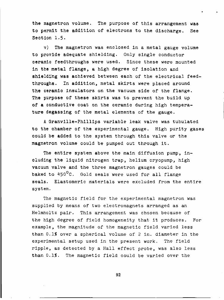
the magnetron volume. The purpose of this arrangement was
to permit the addition of electrons to the discharge. SeeSection 1.5.
v) The magnetron was enclosed in a metal gauge volumeto provide adequate shielding. Only single conductor
ceramic feedthroughs were used. Since these were mounted
in the metal flange, a high degree of isolation and
ahleldlng was achieved between each of the electrical feed-
throughs. In addition, metal skirts were placed around
She ceramic insulators on the vacuum side of the flange.
The purpose of these skirts was to prevent the build up
of a conductive coat on the ceramic during high tempera-
ture degasslng of the metal elements of the gauge.
A Granville-Philllps variable leak valve was tubulated
to the chamber of the experimental gauge. High purity gasescould be added to the system through this valve or the
magnetron volume could be pumped out through it.
The entire system above the main diffusion pump, in-
cluding the liquid nitrogen trap, helium cryopump, high
vacuum valve and the three magnetron gauges could bebaked to 450°C. Gold seals were used for all flange
seals. Elastomerlc materials were excluded from the entire
system.
The magnetic field for the experimental magnetron was
supplied by means of two electromagnets arranged as an
Helmholtz pair. This arrangement was chosen because of
the high degree of field homogeneity that it produces. For
example, the magnitude of the magnetic field varied less
than 0.1% over a spherical volume of 2 in. diameter in the
experimental setup used in the present work. The field
ripple, as detected by a Hall effect probe, was also less
than 0.1%. The magnetic field could be varied over the
92

range of 0 - 2200 gauss with the power supplies available.
In general• however• field variations over the range 400 -
2000 gauss were adequate for most of the experimental work.
The procedure used for determining the main performance
characteristics of the experimental magnetron gauge was as
follows. After thorough degassing of the system and gauge•
a known pressure was established in the experimental gauge.
This was usually done by admitting argon Into a section of
the system above the high vacuum valve. The pressure was
measured by the reference Redhead gauge. The cathode current
from this gauge was converted to pressure (Torr N2) by meansof Fig. ll. Since the latter takes into account the non-linearity of the gauge below 2 x l0 -10 Torr, the reference
pressures quoted in the following discussion correspond to
actual Torr N2. After establishing a definite pressure•the experimental gauge was operated at 1000 gauss and
10,000 v for a period of at least 45 minutes before startlng
a series of measurements at lower anode voltages. This
p_oced_e was _.... _ to give more reproducible results -
particularly at the lower pressures. It is not unlikely
that the gauge nlay tend to clean itself at the higherionization rates.
In the major part of the work, emphasis was not placed
on the measurement of low pressure. It was more to the
purpose to investigate a wide range of variables around
the region where the gauge changes from linear to non-linear.
The main conditions investigated were:
Pressures (Torr N2): 5.2 x l0 -8, 5.2 x l0 -102 7 x l0 -ll 1 2 x l0 -ll
Anode Voltages: 1000 - 8000 in 1000 volt steps.
Magnetic Field Strength: 400 - 2000 gauss in 100 gauss steps.
This program thus covered some 500 combinations of pressure,
anode voltage and magnetic field. The data apply to a magnetron
9S

• q
FIG. ii
CALIBRATION CURVE 552 GAUGE
10-7
10 -8
10-9
CATHODE
CURRENT
(amp)
i0-i]
i0-i_
i0 -12 I0 -II i0-I0 10-9
PRESSURE (Torr N2)
-8i0 10-7
94
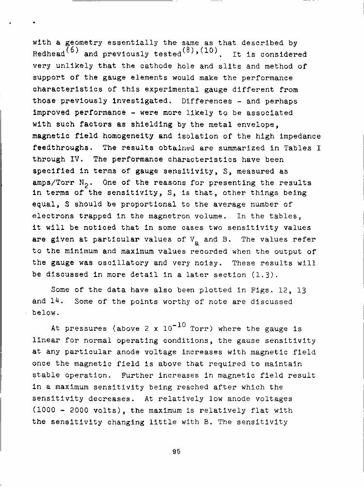
with a geometry essentially the same as that described byRedhead (6) and previously tested (8)'(10). It is considered
very unlikely that the cathode hole and slits and method of
support of the gauge elements would make the performance
characteristics of this experimental gauge different from
those previously investigated. Differences - and perhaps
improved performance - were more likely to be associated
with such factors as shielding by the metal envelope,
magnetic field homogeneity and isolation of the high impedance
• ee_v_ghs. The results obtained are summarized in Tables I
through IV. The performance characteristics have been
specified in terms of gauge sensitivity, S, measured as
amps/Torr N2. One of the reasons for presenting the resultsin terms of the sensitivity, S, is that, other things beingequal, S should be proportional to the average number of
electrons trapped in the magnetron volume. In the tables,
it will be noticed that in some cases two sensitivity values
are given at particular values of Va and B. The values referto the minimum and maximum values recorded when the output ofthe gauge was oscillatory and very noisy. These results will
be discussed in more detail in a later section (1.3).
Some of the data have also been plotted in Figs. 12, 13and 14. Some of the points worthy of note are discussedbelow.
At pressures (above 2 x l0 -10 Tort) where the gauge is
linear for normal operating conditions, the gause sensitivity
at any particular anode voltage increases with magnetic field
once the magnetic field is above that required to maintain
stable operation. Further increases in magnetic field result
in a maximum sensitivity being reached after which the
sensitivity decreases. At relatively low anode voltages
(1000 - 2000 volts), the maximum is relatively flat with
the sensitivity changing little with B. The sensitivity
g5
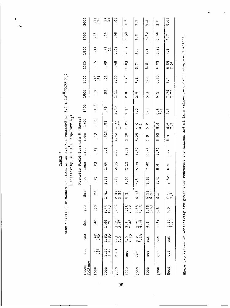
o
ooo.I
ooo_
oo
oo
oo
oo
0 ,-"_c_O
_H• °
-:FH
Lf_ b_-H_• °
O_
Lf_
Od
0Cq
o
o
o_o
• .
k£)0_
• °
ooo,-I
=l-kO
• °
o_
,-Iu_
o_
o,I
ko
_o
,-I
,-I
,-I
,-I--=r
,-I
Lr_ 0-_
,--I ,--I
_00kO_--
• .
kO0_• °
,-4,--I
¢qOJ
• °,--I ,--I
ooo
%
0oo_
,-Io
00
oo
o_
o_o_
H,--I
0
U_
O_
0_0-=r o_1
• °
_o0
• °
• °o.I (_1
0
000
0
L_
o_
0o
o
o
Od
CO
0Dq
0.1
o_
_DC_I
00
,?_!
0
o00
o,I
co
ckl
b--
o
o• °
=1-
Go
• °
t.c_ u_
b-- -.m-
ooo
o,I
o,I
H
00
0
LE_
0
LE_
CO
_D
• °
_0• °
-.-r
0
0
ooo_o
o
o_
o
oo
_o
L_
kO
O_b--• °
kOkO
GO
Od
O0
Lf_
aO
b--
Od
O0
O0
0
0
ooo
od
0o1I_
'_o t'.--
• °[_-b-
_D
L_• °
O0
0
0
O0
t-
• °
O_b-
0
0
000O0
0
0
.,-I
=1
0o
>
=1
"0
0d
(1).el
4-_
4.>c-,
mID%
®%
e-,
>
%
,,,-.I>
0
>
0
%
g6

ooo(%1
oo
o_,-I
c)o(30,-I
oo
,-I
oo
n_O
o o,--4 o
! ,..._o ,-I,-I
X
{'M f,j o
• Z oL(_
O O
LT1 _ O_ _ O
c_ n O o_ _ o
M on ,--I
H M N? O
H _> _ _ O
_ _ _ o,_ _ ,-I o
_ o
O n IT.,:=:)
r_ _ .H Ot- .P O
'7 ,-4 _ O%OE: U _1
O
O _
_ o_ _ o
H CO
I-4 O_ OI--4 _2)r_
OO
O
O
C_10o0_r-t
• °
• °
(._
f_
O
O
Co
Ot_
O
c_
t_0o
O
',o
r-t
,-4r't
O
."t
,o%r_C*
• •
HO
O
r-I
O('_1('MO
0b-
O_
b--
t_o
t_o
,.-4
ooo
• , ° °
• ° ° °
HC_I tl_ e-I
• ° o °
P¢'I r--I GOI_• o • •
_r
• °
o
f_ f_
w4
0
o oo oo 0
ko_• o
co
Lf_
0
_0
• °
• o
_Lf_• °
f_
L_
_0
k__0
_0
b-_O
Lr_
CO
Lr_
O03
0%
f,3
(MLr_
cOO0
O
o0oLC_
C_O_
CO(',-)t- -'_C)
• °
COLC_
t-- C',IOJco
• o
cOO_'.D
• °
COOJ',OOJ
• °
(:OO{3
• °
O0 [---
0
O0
CO
O0
0
0
f_
LC_
HC'J
Lf_
LC_C_
C_
0
0
oooko
cr_
cO
coo• °
OO• °
-..-r ,-I
ko--rc}o t._
• °
coco
co,-i
(3oo.i
co(M
Lr%
O_
O
O,--I
O
LP_
Lr_
b
Lr_
LC_
OkO
,--I
:3O
:3O
ooo
b,-
0o L"--• °
L,_'_,0._
• °*--'1
k.O 0'_
• °
o_
0ood
_-o_• o
cM
o
_M
H
o
_o
cMco
°
b_
_o
_o
o
o
0
0
ooo
co
m
0,rl
oto0
g_
g_0
o
c_
c_
c_
0
g_
4_
t_
0
r_
0
9'7

r_
OE_
I
X
_ or_ E_
_ E
O o_ °
_ M
_ _+1+MO II
-I.-
O
O_ 2N _
O _4.J
H
HE-_F-tr_
Mr.O
Ooo
oochr-I
oo0o
r-I
oob-
oo,-I
oorq
00--:rt--I
0,'1e--t
m o
_ c.4
NI ,-4
%
_oo
_ o
r_
co
o
ot_
ko
oo
0c"
r--I
::_ 0r--I I__
rH U_
,-t
:_- O,-t t_
r-I
,O
r--t
• °
e-I e-I O.I -=:r• ° I ° .
e_ ,--t
,--t
C_I -7'-
,'-I
(M C_I°
r-t
N _
_rn _• ° °
cof_
c_l Pc3• ° .
• °
• ° . °
O0 O0
oo oo clr"t o.1
f,e3
f_
f_
r--I kl_
• °
f',l C',l
%oJ
c,d
,-t
od
r-'t
t_
-=:r
o"_ c'J_ctloo
. °
ooo
._o I-tc_ i• .
-,1 c,d
::r
121
:::r
;::T
• °
f_l iw-i
c,'3 ,.O
_oe3
t-.--
co
O
t'x3
'.D
,--t
ts%
,--t ,-t• .
O O• °
ooo
ch,-H
oo_o
%
-::r
Lr_
CO
Ob--
o_
k4E)
.-t
r--I
_DOOO_OJC_
• °
C_Lf_
C) O• °
OOOO
• °
OOO
2
D
;o
_hc_
b-
,-I
°
o
oc)
b-0o
oo• .
oo
b--c_ooo o
• °
ooo
ko
oLE_
L_C_
OO
C_
,--I
r-I
kO
O
O
oob-
Lf_
O
b-
• °_--I r-I
• °
OOO
r'l ,--IC),-I
• °
b-,--IO,-'tOO
Or-IOO
• °
OOOOO
O.,H
,-t"rl
O
• r'C_ ..H
0 "¢1
"ao,-I 0
, _
,.-.t
c_
4-)
O _
® %
r.,'?
& =
c_r'l II)
O c_ NI
Oh'- _1
_ °
_ ,_ O
% O
,% ,% •
98

ne
O_0E_
, o
_ o_
°_
_ _ 0_ --=r
_ _+_ _ oIll f_
m _
r_ 42_ .el r-I
Z _rt 4-_ 00 m G; r-_
o3
_ o
0
_ o
a
I-4
H 0
tO 0
0 _0 _0 0
o
o
o o_ L_0 0
r_ • • I
• °
I
.::r I ua
• °
_D
• °
,-t r_• °
o _ _
o _ _
_ ° °
o : oo ! oo o_-4 (M
N1
"CI._Or-__0
-..-r
• °
• o
¢--t
Pqb.-
u_
,--t
oo
o
%
ooo
• o
f¢3 _
0% i o_• I "
00_:00
• •
LE_• °
04 _r_
• °
r_l fr3
_ -=I-
• °
_ o• °
o• °
o"3 od• °
o o
e.-I _-t
t'.- _• o
M_• °
• °
• o
0 .-.-1"
c¢3 __ 0
0 00 00 0
'IJ
4_0c,
II
99

0H
0
I
tItI
\
!
/
>000b-'
/
0
o,I
oE_
C
100

Io
b.00
H
I
0
o
Ior--I
L_
II
I
b.o00
I
0
\IQ
I
\o
oJo
/
/I
I
\
r_
0
H
a3
f-t-1t--I
C.)t.--tE_
CD
101

oi---I
\
_ oo t-_ '.D _ _ t_ Od ,-4
o
o
o_
OD
b-
oo
102
t-
also increases with anode voltage and the results presented
in Figs. 12 and 13 suggest that there is an upper limit or
envelope for the sensitivity at values of B less than those
for maximum sensitivity at any particular anode voltage.
This upper limit or asymptote is approximately linear with
magnetic field. The slope appears to be somewhat higher
at 5 x l0 -8 than at 5 x l0 -10 Tort. However, this may
be associated with the fact that the gauge was much
noisier at 5 x l0 -8 Tort at low values of B than at 5 x l0 -10
Tort. This contrasted sharply with the situation at higher
magnetic fields after the maximum sensitivity values had
been reached. At 5 x l0 -8 Tort the sensitivity dropped
relatively slowly and there were few conditions where
noise and oscillations were noted. At 5 x l0 -10 Tort, the
sensitivity decreased abruptly after the maximum and there
were many conditions where the sensitivity oscillated as
indicated by the output from a Keithley 410 electrometer.
There were, in addition, a few isolated conditions at high
magnetic fie __s where the gauge returned to relatively
high sensitivity. Some of the aspects of this oscillatory
behavior will be described later under Section 1.3.
The above results follow the same general pattern as
those of Redhead (ll). The high sensitivity region at low
magnetic fields corresponds to Redhead's State I and the
lower sensitivity at high magnetic fields corresponds to
State II. The above results pertain to pressures above
2 x l0 -10 Torr. At lower pressures where the gauge is
non-llnear, the general nature of the curves appears to
change drastically (Fig. 14). The rate of increase of
sensitivity with magnetic field is much lower than at
the high pressures.
At 2000 volts and 3000 volts the sensitivity is con,
stant for a large range of values of the magnetic field
strength. There is also some evidence of a flat maximum in
103

_V
sensitivity being achieved at 700 gauss and I000 volts. The
general nature of the curves in Fig. 14 suggests that at the
higher anode voltages, e.g., 6000 - 8000 volts, magnetic
fields in excess of 2000 gauss would produce a range of con-
stant sensitivity. It is not unlikely that even higher
magnetic fields would give decreased sensitivity. The effect
of magnetic field and pressure on the sensitivity at an
anode voltage of 5000 v is shown in Fig. 15. At 5 x i0 -I0
Torr, the sensitivity is a maximum at about II00 gauss. (Note
that at 5 x 10 -8 Tort the maximum at 5000 volts was at about
800 gauss. See Fig. 4.) At both 2.7 x i0 -II Torr and-Ii
1.2 x i0 Tort no maximum is shown. The variation in
sensitivity is approximately linear with magnetic field
at 2.7 x l0 -ll Torr and 1.2 x l0 -ll Torr. The slope
decreases with pressure.
It should also be noted (Fig. 13) that at a magnetic
field strength of, say, 1500 gauss the gauge sensitivity
is greater at 2.7 x l0 -ll Torr and 1.2 x l0 -ll Torr than
it is at 5 x l0 -10 Torr. Similarly, at 1500 gauss and
5000 volts the sensitivity is greater at 2.7 x l0 -ll Tort
than at 5 x l0 -8 Torr.
If it is assumed that the number of magnetically
trapped electrons (N) is proportional to the sensitivity,
the above results indicate that at the specific conditions
taken above, N is lower at the higher pressures where the
input rate of electrons from the volumetric ionization
process is greater. In general, it would be expected
that the higher input rates would tend to add to rather
than subtract from the number of trapped electrons. In
this situation, one is tempted to seek an explanation in
terms of the r-f oscillations which have only been
detected at the higher pressures (Redhead). _ll_'_ It
might be assumed that these oscillations effectively reduce
the number of trapped electrons. However, as is shown by
104

• /
0
,---I
I I
oOctD
_H
_H
_H
H_
OZHO
_,_
H
I i
' \
,,,H
n ' . _ _ I,,I
o _ _ \ _
_L \ \ _
_ ,, \_
\\ I-
\\
i i i I I I .I ._ l _"'_ _ _ _ C_I r-_
o
cd
0
C_
r--_
r-_
r-I
C_
r'-I
C_
rM
0
r-i
o_
o
o
o
o
L_
0
0
_._0
I-I
;-I
H
c)H
Zc_
105
Redhead, (I0) it is likely that the r-f oscillations are asso-
ciated with the rotation of the electron cloud. Hence, at
the same values of Va and B it is more difficult to see why
increasing the electron production rate(and loss rate)
by increasing the pressure should cause oscillations to
develop in the electron cloud. The simpler explanation that
the oscillations are dependent only on V A and B and essen-
tially independent of pressure - above 2 x l0 -10 Torr- seems
more acceptable. Further work should be carried out to
measure the frequency and relative intensity of the oscilla-
tion under conditions of equal gauge sensitivity. It may
well be that strong r-f oscillations do in fact exist at,
say, 2.7 x l0 -ll Tort, 1500 gauss and 5000 volts. It is,
nevertheless, possible that the ion c,r_ent is far from
constant at any pressure and that there are growth and
decay processes continually taking place in the electronic
space charge. At high pressures (above 2 x l0 -10 Torr),
these processes which are probably associated with surface
reactions at the cathode and anode possibly initiate
or produce distortions in the electron cloud which result
in stable r-f oscillations. At low pressures, the surface
controlled initiation processes may be too small to produce
oscillatory behavior.
From the data presented in Tables I through IV it is
a simple matter to determine those sets of conditions at
which the gauge has the same sensitivity at various pres-
sure. That is, the conditions under which the gauge is
linear. The results are presented in Fig. 16.
The data associated with line A in Fig. 16 where ob-
tained by plotting those conditions at which the sensitivity
at 5.2 x l0 -8 equal that at 5 x l0 -10 Tort. Line B was for
conditions where the sensitivity at 5.2 x l0 -8 Torr equaled
that at 2.7 x l0 -ll Torr. Along both line A and line B,
106
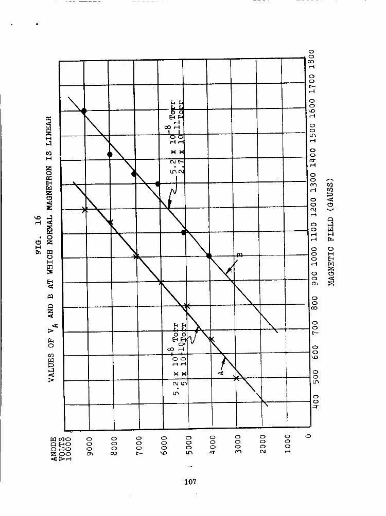
H
\\
CO 4I.-i
ZO
I.-t
C_I-t
E_
Z
0
\
\1
,1
L, c.O0
,--ICOr-I
I IO0,--I ,-I
a+ t--.
I
\-\
_a _a0 0
Oor--I r-_
t'_ ,
\\
O_O O O O O O O O OI_1 [-_O O O O O O O O OO1--10 O O O O O O O O
OO O_ CO t_- _O I._ --.1" O'_ _1
,i,,i ,J
\
i. iii
ooo,-I
oo0or--I
00b.--,--I
oo
:_or--I
ooL_r-.I
0
00
00
00+--Ir-I
000r'l
00
00CO
00
00_£)
00
00-::1"
0
CO
v
I--I
r..)H
:z;
E
10'7

the sensitivities increased with anode voltage (and magnetic
field). Line A is approximately parallel to line B, and
at any anode voltage, line B is located at a magnetic field
strength which is approximately 350 gauss higher. The
normal operating conditions for the 552 magnetron gauge are
i000 gauss and 5000 volts. This lies on line A. The data
of line B then suggest that at, say, 3000 volts and ii00
gauge, the magnetron gauge would be linear down to at
least 2.7 x i0 -II Torr. Thi_ requires that the cathode
current vary monotonically over the pressure range
5.2 x l0 -8 Torr - 2.7 x l0 -ll Torr. A number of pressure
variation tests were carried out at 3000 volts and ll00
gauss and also at 4800 volts and 1250 gauss. The results
for 3000 volts and ll00 gauss are presented in Fig. 17.
The best line through the data gives a slope of 0.90 down
to approximately 1 x l0 -10 Tort. At lower pressures there
is evidence that the slope increases to approximately 1.8.
_, The data for the lowest two pressures were taken from
separate experiments as recorded in Tables III and IV.
The slope obtained in this work in unusual in that it is
less than one. It is possible that the Reference gauge
changed from a slope of 1.0 to something less, but this is
unlikely. However, the decrease in sensitivity from 2.15
amps/Torr at 2.7 x l0 -ll Torr to 1.0 at 1.2 x l0 -ll Tort
(see Tables III and IV) indicates that operation in State II
is not likely to give high sensitivity performance at very
low pressures. The data taken at 4800 volts and 1250 gauss
also gave a slope of 0.90. Interpolating from the data in
Tables III and IV indicated that within experimental error
the slope remained constant down to the lowest pressure
measured, 1.2 x l0 -ll Tort. However, a comparison of the
data in Tables III and IV at higher anode voltages and
magnetic fields shows that there is a decrease in sensitivity
at the lower pressures. This is also clearly shown in Fig. 15.
108

FIG. 17
NORMAL MAGNETRON CATHODE CURRENT
VS. PRESSURE (3000v, ll00 GAUSS)
r-%
z
o
o
30 -8
10-9
-]i0
l0 -1 10-11
/
SLOPE .90
/
FROM TABLE III
FROM TABLE IV
0
//
/
I0 -I0 10-9 10 -8 10-7 10 -6
PRESSURE (TORR N2)
109
The data at 4800 volts and 1250 gauss showed considerably
more scatter than the data of Fig. 17. Some of the scatter
obtained in the early part of the experiment was found to be
affected by the R, L, C of the electrometer circuit. For
instance, at some specific pressures, particularly in the
range 6 x l0 -10 Tort to 2 x l0 -9 Torr, a 410 Keithley
electrometer would oscillate between specific values. A
study of some of this oscillating behavior indicated that
several types of oscillatory behavior may be observed when
measuring pressures in State II. These are discussed more
fully in the section below.
110
1.3 OSCILLATORY BEHAVIOR
Redhead (ll) has given an extensive description of the
r-f oscillations which exist in the magnetron gauge when
operated in State II. Redhead's results on the effects of
magnetic field strength and anode voltage in the frequency
have been confirmed in the present program. The specific
frequencies have been observed in a number of ways including
field intensity meters, tuned r-f receivers and by means
of __ .._h_g_....e_,_'-_-..._jo_^_^ope__ . _±_ coupling may be
carried out in a number of ways, including direct coupling
to the auxiliary cathode on main cathode, capacitive
coupling to the anode or by means of a small antenna
supported axially near the gause anode.
One of the aims of the present program was to measure
the variation in intensity of the r-f signal as a function
of pressure. Redhead has reported that the r-f oscillations
were not detected below 2 x i0 -I0 Torr. A number • of attempts
were made to measure the effect of pressure on the signal
intensity but with little success. Using a tuned r-f
receiver and a signal intensity meter some data (Fig. 18)
were obtained which tended to suggest that the maximum signal
intensity at any pressure decreased as the pressure decreased.
At no time was an r-f signal detected below 2 x l0 -10 Torr.
However, the data showed considerable scatter and cannot be
regarded as more than minimal evidence. In this part of the
work, experimental procedures were greatly hindered by an
exceedingly strong 80 Mc/s signal from an external source
beyond our control. The metal system Helmholtz coils,
electrical and cooling water systems all acted as antennae
for the signal. Attempts to filter the signal and its
harmonics were not successful and it was beyond the limita-
tions of the program to install adequate shielding.
111
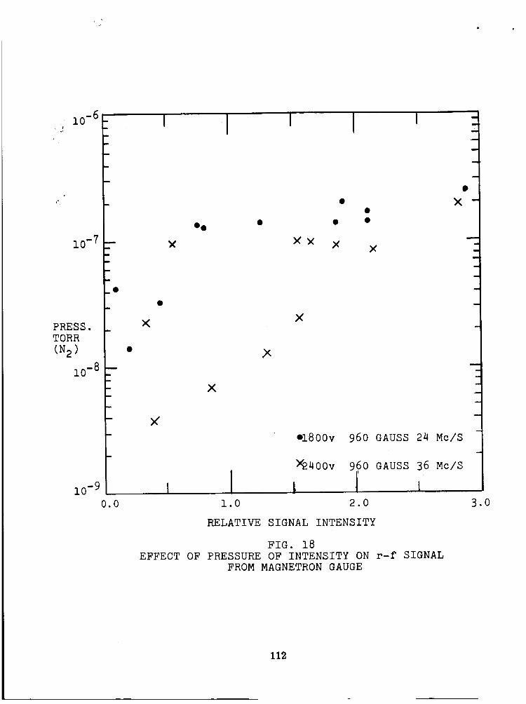
lO-6• r
10-7
PRESS.
TORR
(N 2 )
lO-8
10-9
B
l
m
w
m
n
m
m
_@
@
X
X
@@
[
X×
X
X
m=
Lm
.U
m
@
× -
m
m
a
i
0.0
m
- >_
×
M
N
a
el800v
_2400v
I
960 GAUSS 24 Mc/S
960 GAUSS 36 Mc/S
I2.0 3.0
RELATIVE SIGNAL INTENSITY
FIG. 18
EFFECT OF PRESSURE OF INTENSITY ON r-f SIGNAL
FROM MAGNETRON GAUGE
112

When operating in State II a different type of oscillatory
behavior was noted. In this case, electrometer oscillations
would develop above and below previous mean steady state values.
The frequency was on the order of 0.1 - 1.0 cycles/sec. The
period of the oscillation increased with decreasing pressures.
These types of oscillations were often evident with an electro-
meter such as a Kelthley 410. If the input capacitance of
the electrometer was reduced, as with a Kelthley 600 or 610
operatlnE in the fast mode, oscillations did not occur. The
R-C constants of the entire electrometer circuit should be
such as to eliminate such low frequency oscillation. The use
of a high quality vacuum capacitor to shunt high frequency
components of the cathode current to ground is recommended.
113

1.4 EFFECTS OF ULTRA-VIOLET RADIATION
A convenient method of decreasing the starting time of
a magnetron gauge at low pressures is by irradiating the
gauge with ultra-violet. The mechanism by which photo-
radiation assists in initiating the build up of the discharge
has not been determined. One, or a combination, of the follow-
ing processes may play a part.
i) Photo-emisslon of electrons from cathode.
li) Photo-desorption of neutral gas species previously
adsorbed on gauge elements, walls, etc.
Ill) Photo-ionlzation of a neutral, free or absorbed gas
species.
Experimentally, it is not easy to differentiate between
these processes and other effects - especially thermal de-
sorption effects associated with the radiation. However,
if the non-linearity of the magnetron gauge is caused by
a deficiency in the number of electrons in the discharge,
an increase in the number of electrons emitted by the
cathode should tend to make the gauge more linear. Bryant _7j""
has shown that a ceslated magnetron gauge has a non-llnear
characteristic, which has a lower slope than an uncesiated
gauge. Presumably, lowering the work function of the
cathode results in at least a partial increase in the number
of desired electrons in the discharge• As a practical
procedure for low pressure work the use of cesium has
obvious drawbacks• Another possibility of testing the
electron deficiency thesis appeared to lie in attempting
to stimulate photo-emlssion by the use of ultra-vlolet.
The radiation from a low-pressure mercury lamp, was shone
through the sapphire window of the experimental gauge.o
The output of the mercury lamp peaked at 2537 A and the
sapphire window had a limit of transmission of abouto
1400 A (9 ev). Typical results were as follows: At a
114

pressure of 3.7 x i0 -II Torr the output current of the gauge
rapidly rose from 6.8 x l0 -ll amps to 9.8 x l0 -ll amps. Within
5 minutes it decreased from this value and leveled off at
7.5 x l0 -ll amps. It remained constant at this value for as
lone as the u.v. lamp was on (2 hrs.). However, this 10%
increase in the output of the magnetron gauge was too small
to be attributed to an increase in gauge sensitivity. Even
though thls was a steady increase in output current, it is
more likely that it was caused by thermal desorption of gas
which was temperature and not time dependent. In any case,
even if it were all attributed to an increased gauge
sensitivity, the increase is only 12% of that required to
give a linear gauge. More work using a system in which a
concentrated beam of ultra-vlolet radiation is focussed on
specific areas within the gauge is recommended. In this
work, temperature variations should be investigated to alter
the effects of thermal and photodesorption of physically
adsorbed gas. It is, however, llkely that the magnetron
discharge is already an efficient source of ultra-violet
and X-ray radiation so that external sources may only have
secondary effects.
115

1.5 ELECTRON INJECTION
As shown in Fig.10, the experimental magnetron was de-
signed so that an external filament could be used to inject
electrons through a small hole in one of the cathode end
plates and along the lines of magnetic flux. The hole in
the cathode end plate was 1/8 in. diameter and its center
was located 1/3 of the distance from the surface of the
central cathode rod to the anode diameter. The tungsten fila-
ment was coiled to an O.D. of about 0.08 in. In order to
prevent electrons moving directly to the cathode, it was
first necessary to determine the bias required on the
filament supply to prevent this. This was done with the
magnetron gauge not operating (Va - 0) but with the range
of B fields planned for experimental use. With the filament
at 1050°C, it was found that a bias of 4 volts was sufficient
to reduce the electron current to the cathode to less than
5 x l0 -14 amps. The gauge was then degassed by electron
bombardment and the temperature of the filament raised to
1350°C for about 1 hour. The output current of the ex-
perimental gauge was then measured with the filament at
1050°C and biased 4 to 6 volts above ground. At a pressure
of 3 x l0 -ll, these conditions caused an increase in the
cathode current of about 10%, but once again it is doubtful
whether this current could be attributed to an increase in
gauge sensitivity. Even though very careful degassing
procedures had been used, the magnitudes of the pressure
changes in the experimental and reference gauges were
commensurate with increased thermal desorption rates in the
gauge.
Since the electric fields within an operating magnetron
gauge are not known, it is difficult to inject electrons
into the discharge. If the electrons do not have sufficient
energy, they will not penetrate to the discharge. If they
116
have too much energy, they will pass through the discharge to
the opposite cathode plate. In a later model of an experi-
mental gauge, a small accelerating grid was placed between
the filament and the cathode plate. It is anticipated that
this may allow more control and perhaps permit adequate
testing of electron injection techniques. It may be advan-
tageous to place holes in both cathode plates so that
electrons with excess energy would not be collected by the
back cathode plate but would move on to a dummy cathode
behind the hole in the true cathode.
117

1.6 PHOTOGRAPHIC STUDIES
If a normal magnetron gauge is allowed to operate at
-4 l0 -5 Torr - arelatively high pressure - say l0 or
characteristic purple glow is clearly visible within the
gauge. In a darkened room, this glow is still discernible
at much lower pressures, particularly if l0 or 15 minutes
is allowed for eye accommodation. It was the aim of this
part of the program, to attempt to determine the distribution
of the discharge within the gauge by photographic techniques.
It was hoped that not only would it be possible to map the
discharge within the linear region of the gauge but that
the techniques could be made sufficiently sensitive so that
the distribution below 2 x l0 -10 Torr could also be deter-
mined.
The experimental magnetron gauge, Figure 10,was assembled
so that one of the cathode end plates could be viewed
directly through the sapphire window in the flange of the
magnetron chamber. A radial slot (1 mm wide) was cut in
the cathode end plate from the outer edge to within 1.4 mm
of the central cathode rod. A mirror was also mounted at
approximately 45 degrees to the magnetron axis outside the
anode screen. However, this mirror was of limited usefulness
in measuring the axial distribution of the glow because of
parallax problems associated with the relatively small
sapphire window. It was experimentally easier to photograph
the axial distribution directly through the glass of the
reference gauge, a NRC 552 gauge.
Most of the photographs were taken with a Linhof Technika
Camera, using Xenar 1:4.5/150 lens. For the major fraction of
the work, Polaroid Type 57 film (ASA 3000 speed) was most
suitable. At the lower light levels, Polaroid Type 410
(ASA speed 10,000) was also used. In general, the camera was
operated with a lens opening of f 4.5 at approximately 7 in.
118

from the magnetron assembly. The resultant image had amagnification of 1.47. When taking photographs of the
experimental magnetron, the shutter mechanism failed to
operate in the high magnetic fields associated with the
Helmholtz pair. However, time exposures were generally
necessary so that it was entirely satisfactory to use
plate slides to give the desired exposure.
The main part of the experimental work was devoted to
the determination of the effects of pressure, magnetic
field strength, anode voltage and gas composition in the
shape, location and intensity of the discharge. Themajor results are summarized below.
A representative photograph of the radial variation
of the intensity of the discharge is reproduced in Fig. 19.The figure is a view of the discharge at 4.2 x l0 -6 Torr
through the radial slot in the cathode end plate. Theslot extended from the anode to within about 0.07 in of the
surface of the central cathode rod. The photograph shows
that the glow extends from the surface of the cathode rod
to about half way out to the anode. The intensity appears
to be relatively constant to approximately 1/2 (r a - r c)and it then drops rapidly to a negligible value. Photo-
graphs of the discharge as seen through the perforated anodewere used to obtain an estimate of the axial distribution
of the discharge. By taking a series of photographs at
slightly different angles, various sections through the
discharge could be photographed. This series of photo-
graphs, when taken in conjunction with the radial photo-
graphs, has suggested that the distributions within the
gauge are as shown in Fig. 20.
The discharge extends out from the cathode rod to about
half the anode distance. The axial length of the discharge is
considerably less than the distance between the cathode end
119

LENGTH
0F@SLOT
SLOT WIDTH
ANODE
CATHODE
MAGNIFICATION 1.47
FIG. 19
VIEW OF DISCHARGE THROUGH RADIAL SLOT
IN CATHODE OF MAGNETRON GAUGE.
GAUGE CONDITIONS: ANODE: 4800V
MAGNETIC FIELD i000 GAUSS
PRESSURE 4.2 x 10 -6 TORR
120

ANODE
REGIONS OFMAXIMUM
INTENSITY
CATHODE
FIG. 20
DISTRIBUTION OF PHOTO-RADIATION FROM
MAGNETRONGAUGE
121

plates. That is, the discharge does not appear to extend to
the cathode end plates. The general shape of the discharge
resembles that of a doughnut around the cathode rod. There
was some evidence that the maximum light intensity was not
at the cathode rod but somewhat removed from it, as shown
in Figure 20. However, this increase in intensity was
relatively small. The axial length of the discharge appears
greatest at the cathode rod so that the radial sections
appeared to give an intensity which was either constant
out to 1/2 (r a - r c) or at a maximum at the surface ofthe cathode rod.
The above results were obtained with the gauges operating
in Argon at 4.5 x l0 -8 Tort (N2) at normal conditions - anode,4800 volts; magnetic field, 1000 gauss. The effects of
variations in pressure, magnetic field, anode voltage and
gas composition are summarized below.
Photographs obtained of 4.5 x l0 -7 Torr, 4.5 x l0 -8 Torr
and 4.5 x l0 -9 Torr indicated that the intensity of the dis-
charge was directly proportional to the cathode current.
Quantitative densitometer measurements of the intensity of
the discharge were not made but by varying exposure times
at different pressures and using visual comparison of the
photographic density, a fair estimate of the degree of
proportionality could be obtained. Future work would begreatly facilitated by densitometer measurements. In orderto obtain a reasonable picture of 4.5 x l0 -8 Torr, an
exposure time of l0 minutes was required with the 3000 speed
film. Unfortunately, no photographs of the dischargewere obtained in the non-linear region below 2 x l0 -10 Torr,
even though exposure times in excess of 12 hours with
10,000 speed were used. Unfortunately, the films used lose
reciprocity for exposure times greater than about 8 hours
so that larger exposure times are not beneficial.
122

The effect of varying the anode voltage was investigated
at two levels of magnetic field - 1000 gauss and 500 gauss.
The pressure was 4.5 x l0 -8 Torr and the gas, argon. In
order to compare the results, an arbitrary scale has been
used to estimate and specify the intensity. A range of 1
through l0 was used for l0 minute exposures of 3000 speed
film. Intensity 1 was barely discernible - and l0 was
complete exposure of the film. Intensities outside this
range were obtained with exposure times other than l0
minutes.
In some instances, considerable variations in film
sensitivity were noted from pack to pack. In general,
fresh packs were used for each series of experiments and
there was then good consistency within a series. Where
comparison between series was required, the estimated
sensitivities were normalized so that intensities at
5000 volts and 1000 gauss were consistent. The results
have been summarized in Table V. The distance which
the discharge extends out from the cathode is specified
in terms of R - the fraction of the cathode to anode
distance from which light is emitted.
TABLE V
EFFECT OF ANODE VOLTAGE (V A) VARIATIONSON INTENSITY OF DISCHARGE IN ARGON
Pressure VA B i+Exp.
(Torr N_) (Volts) (Gauss) (Amps)4.5x10 -o 7.4x10-78000 1000
7000 100060O0 1000
50OO 10004000 1000
30oo i0o0
4800 5O0
45OO 50O
4OO0 50O
3OOO 5O0
20OO 500
lOO0 50O
6.5xlO-7
5. OxlO-7
3.6xlO-7
3.1xlO-7
1 5xi0-7
1 9xlO -7
1 9xlO-7
1 5xi0-71 2xlO-Z10xlO- 2 5xlO -_
Relative
R Intensity
•53 15
•55 12
.51 9
.52 7.5
.52 3
.36 1.2
.48 7.5
.54 12.0
•53 9.O
.51 6.O•55 6.O
nd. .6
123

In Figure 21 an attempt has been made to estimate the
variation of the light intensity as a function of the radial
position. There appears to be a rapid decrease in intensity
at about half the radial distance to the anode. Increased
anode voltage resulted in higher intensities but this
increase was greatest at the cathode. At 5000 and 6000
volts, the intensity appeared to be relatively constant
for a considerable fraction of the distance out from the
cathode. The results obtained on varying the magnetic
field from 600 to 2400 gauss are summarized in Table VI.
Pressure
(Torr N2 )
TABLE VI
EFFECT OF MAGNETIC FIELD VARIATIONS (B)ON INTENSITY OF DISCHARGE ON ARGON
VA B i+ Exp. R Relative(Volts) (Gauss) (Amps) Max. Intensity
4.5xl0-STorr 4800 600 2.0xl0 -7 .52 5
4800 800 2.9xi0-7 .58 7.54800 i000 2.2xi0-7 .56 7.0
4800 1200 2.5x10⁻⁷ .59 8.0
4800 1400 1.4xlO-7 .51 6.3
4800 1600 1.4xi0-7 .58 6.54800 1800 1.2xlO -7 .58 6.1
4800 2000 1.15xlO -7 .56 6.0
4800 2400 1.15xlO-7 .56 6.0
In Figure 22 an attempt has again been made to estimate
the variation in the radial light intensity as a function of
the magnetic field intensity. It is noteworthy that the
gauge has the highest sensitivity at 1200 gauss - a condition
where the intensity was the highest and constant for a
considerable fraction of the radial distance. At both higher
and lower magnetic fields the intensity was lower, and
appeared to decrease continually from the maximum value at
the cathode. In general, the areas under the curve
correlated with the gauge sensitivity - except at
extreme values. For instance, the sensitivity of the gauge at
124

FIG. 21
EFFECT OF ANODE VOLTAGE ON RADIAL
DISTRIBUTION OF LIGHT
ARGON 4.5 x 10⁻⁸Torr
B = 1000 GAUSS
H
H
H
H
OQ
14
I I I I
12
l0
VOLTS
6000 VOLTS
5000 VOLTS
8000 VOLTS
4000 VOLTS
0
0
CATHODE
I0.1
3000 VOLTS
0.2 0.3 0.4 0.5R
R = FRACTION OF CATHODE TO ANODE DISTANCE
125

o
t0
oo
I 00
o
h_.
E_H
r.zl _ H
o
o
t_)
O3H
o
o
o
o
o
oI.-I
c)
II
126

600 gauss was 74% higher than at 2400 gauss. However, the
data suggest that increased sensitivity of the gause is
associated with higher intensities of the discharge at
larger distances from the cathode.
In all of the work reported above, argon was used.
Photographs were also taken for helium and hydrogen.
These gases were chosen because they have spectra which
are very significantly different from each other and argon.
When the gauges were operated at the same cathode current
levels, there was no significant difference in the shape
of the discharge. However, the intensity of argon was
greater than that of helium which in turn was greater than
hydrogen. The relative intensities at 4800 volts, i000
gauss in 4.5 x 10 -8 Torr N 2 were estimated as follows:
argon 7, helium 3, and hydrogen 2.
The main results of the photographic studies may be
summarized as follows:
i) In the linear region of the gauge, the glow is
located around the cathode rod. It extends about half way
to the anode but not to the cathode end plates. It is
roughly doughnut shaped.
il) The intensity is approximately constant within the
major part of glow region. The intensity appeared to be
more nearly constant at those VA - B conditions which gave
highest gauge sensitivity, e.g., 4800 volts, i000 gauss.
iii) The intensity is a strong function of pressure. It
appeared directly proportional to the cathode current.
iv) The location and intensity of the discharge appeared
to be essentially independent of anode voltage and magnetic
field. Any change in intensity observed on varying either
the anode voltage or magnetic field could be attributed to
the change in the cathode current.
127

v) It was not possible to obtain photographs of the dis-
charge below the linear region of the gauge.
The fact that the intensity of the emitted light is
directly proportional to the cathode current suggests that
the glow is in fact directly associated with the ionization
process. While a number of possible processes may be
suggested to account for the generation of light, the
simplest overall explanation is probably as follows. Within
the glow regions, electrons have the required energies tocause ionization. Some of the excess energy of the electrons
then appears as photons after the impact
e + A ÷ A+ + e + e + y.
The fact that the intensity appears relatively constant
within the discharge at the optimum operating parameters
of the gauge suggests that the volumetric ionization rate
is constant and therefore the electron density is approxi-
mately constant in its glow region. It also suggests
that the magnitudes of the radial electric fields within
the glow region are relatively small, and most likely
constant. This is consistent with the fact that the volume
of the discharge was essentially independent of the anode
voltage. This would result in constant values of the2Em
cycloidal diameter, d = _ for the electrons in the glow
region. It is interesting to note that the glow appears
to extend out to slightly beyond the radius value
(0.45(r a - rc))at which the radial electric field is a
minimum for the space charge free case. (The space charge
free potential distribution has been measured by Redhead (12)
using electric analogue techniques.)
The above interpretations are largely dependent on the
assumption that the region of ionization is essentially con-
fined to the region emitting the light as evidenced by the
128

photographic techniques. However, the apparent limitation of
the useful discharge to within about half the cathode-anode
distances may have other explanations. For instance, it was
not unlikely that significant radiation was emitted beyond
half the cathode-anode distance, but that it was absorbed in
either the camera lens or the film. Tests with a pinhole
camera did not resolve the problem because the fllm gelatinO O
starts _ _hsorb at 3200A and reaches a maximum at 3000A.
What is required is a hlgh speed film with special sensitivity
down to at least 1800_. It Is not unlikely that such a
film will shortly be available commercially.
In one overexposed photograph of the radial distribution
taken at 5 x l0 -7 Torr, a dark space was observed between
0.73 and 0.82 of the cathode-anode distance. However, beyond
0.82, a faint glow was evident. The intensity of the light
In the anode region was at least an order of magnitude
lower than measured closer to the cathode. However, it
does raise the question as to whether the dark space was
attributable to gelatin absorption and that anode glow was
perhaps associated with light with a wavelength of lesso
than 3000A where the gelatin has a higher transmisslvity.
If this is the case, it would appear that there are con-
sistent radial variations of the spectral distribution.
However, the use of filters with cut-offs above 3200A did
not indicate that the above was in fact the case_ Because
of the nature of the ionization process, it is unlikely
that the emitted light would be a single function of the
radial position. Further work with a film of such
spectral sensitivity would be warranted to resolve this
question.
129

1.7 ANOMOLOUS CURRENT STUDIES
Pressure measurements in the XHV range are made difficult
by the problems associated with reliable low current measure-
ments. The highest sensitivity pressure sensor at present
available in this region is the cold cathode magnetron gauge.
At pressures below l0 -13 torr, a readout current of less than
l0 -14 amp must be measured.
A number of possible sources of erroneous current can
effect the reliability of low pressure measurements. These
are related to four fundamental electrical oroperties of glass
and ceramic insulators used as vacuum feedthroughs_ 3_ They are:
Volume Electrical Resistivity - The volume resistivity
of a dielectric has two components_ 4 The first is the usual
conduction term similar to that for metallic conductors which
obey Ohm's law. The second term is associated with a transient
current which may be many times greater than the conduction term.
The net result is that dielectrics exhibit a conduction current
which not only depends on the applied voltage and temperature,
but also on the elapsed time after the initial application of
the voltage. This time dependence is also effected by the
electrical and thermal history of the dielectric.
Surface Electrical Resistivity - The adsorption of a film
of extraneous impurities on a dielectric surface will generally
result in a decrease of its electrical resistivity. The
adsorption effect can be significantly reduced by chemical
cleaning and bakeout prior to pressure measurement. In addition,
when charged particles come into contact with a dielectric
surface a similar effect can take place.15'16 Results of eXper_
mentally induced surface charging of a borosilicate glass by
Muray show that millisecond time constants for resistance changes
were obtained in a 10-8torr background vacuum. These measure-
ments were carried out at stress levels in the dielectric of up
130

D
to 600 volts. The effect of surface charging in the l0 -14 amp
range and at XHV pressure has not yet been investigated.
Dielectric Constant - The dielectric constant is effected
by dielectric absorption in a way similar to the effects des-
cribed for volume electrical resistance. The dielectric ab-
sorption current, as will be shown, is caused by the finite
time required for dielectric dipole moments to accommodate their
orlentatlon to the applied fleld. 17
Dielectric Strength - In normal operation of the Redhead
Gauge, the pressure dependent ion current is measured between
the main cathode and ground. The auxiliary cathode is held
at ground potential. The potential difference between measuring
electrodes and ground is approximately 1 mV in the lowest pres-
sure range when conventional electrometers are used. Hence,
induced current in a dielectric due to high voltage breakdown
is not of interest in XHV pressure measurement due to the low value
of applied voltage.
This section of the report deals with influence of the
dielectric absorption current in the insulation region separating
the main cathode and auxiliary cathode electrode on electro-
meter currents in the l0 -14 amp region. Surface resistivity
effects were not investigated although a complete evaluation
of this effect is suggested.
Dielectric polarization phenomena result when charges
are displaced interior to a dielectric. Two types of dipoles
may result:
i Permanent dipoles interior to the dielectric material,
which are randomly oriented without the field, but
which may be selectively oriented when the field is
applied.
li Induced dipoles created by the application of the
external field.
131
For the purposes of this report, gases and liquids will not
be considered. In solids, if molecules with permanent dipole
moments are allowed to rotate, however small, they can con-
tribute to the total polarization by increasing the number and
degree of alignment with the increased external field.
Induced dipole moments occur only in the presence of the
applied field. The value of the dipole moment induced in the
dielectric depends, among other things, on the magnitude of
the applied field. The induced dipole may be caused by three
types of interaction of charge particles with the applied field.
The first of these is the distortion of ionic bonding by the
applied field. This is often referred to as atomic polari-
zability, and is caused by the relative motion of ions in
the solid material. The second source is caused by the
deformation of the electron cloud at individual atom sites.
In this type, the center of charge of the electron cloud is
displaced from the nucleus. This type of polarization is
often referred to as the electronic polarizability of the
solid. The third type of induced dipole moment is cause-
by the movement of free electronic and/or ionic charges in
the applied field. If the movement of the free charge is
restricted at crystalline boundaries, a dipole moment will
result, but if the charges move freely to the electrode
then a component of the dc conduction results.
The total effect of both permanent dipoles and induced
dipoles in the dielectric is to create an average dipole
moment associated with the dielectric which depends on the
applied field. This dipole moment is given by:
m
u=aE
where _ = the average dipole moment per molecule
= the total polarizability
E = the local electric field.
132

G •
where:
The total polarizability is given by:
a = md + aa + de + of
md = the polarizability for permanent dipoles
aa = the polarizability for induced ionic dipoles
ae = the polarizability for induced electronic dipoles
af = the polarizability for induced free dipoles.
The +^.oi _,.,.1o...,_,.,_,,-4,.,_, ..,4....
F=NaE
where:
N = the total number of dipoles in the solid dielectric.
From macroscopic theory, it can be shown that
K* - 1 4_
K* + 2 3
where
K* = the complex dielectric constant
E = the externally applied field.
This equation defines the relationship between the
polarizability and the complex dielectric constant K*.
When a constant electric field is applied to a set of
condenser plates which have a dielectric placed between them,
the resulting electronic dipoles induced in the dielectric
material are oriented almost immediately. This polarization
is often referred to as P® (the initial polarization or
the polarization at very high frequencies).
The polarization will increase gradually as the orienta-
tion of the dipoles or the displacement of the ions takes
133

place. This increase will continue until equilibrium is established
approaches the static polarization condition, 18'19and the dielectric
Po' The equation describing the change in polarization in the
dielectric with time is given by:
Pa = [Po - P®][I - exp.( t-to)]T
where T is the well known relaxation time for this process (see
Figure 23). The polarization process is analogous to a
diffusion process where the relaxation time T is given by:
T = TO
eq/KT
where q is the activation energy and To is determined by
calculating the vibrational frequency of particles in a potential
well and is of the order of l0 -13 sec.
To determine if volume polarization effects substantially
influence the current readings in Redhead Gauges at low current
levels(<10 -14 amps) the experiment shown in Figure 24 was per-
formed. In this experiment low voltage pulses were applied
between the auxiliary cathode and the main cathode of a model
552 Redhead Gauge. Typical charging and discharging procedure
was as follows: l) open $2, 2) close S1, 3) short input of
the electrometer, 4) allow a charging period of 1 - 40 minutes,
5) open the input to the electrometer, 6) short $2, 7) open
S1, 8) observe the decay of current recorded by the electro-
meter.
This procedure assured that the full battery voltage would
not appear across the input terminal of the electrometer. The
potential divider network of the supply was designed to allow
its output terminal to be grounded without significantly reducing
the battery emf. The voltage pulses applied were between 0.1
and 0.5 volts in amplitude for periods of time not less than
1 minute. The gauge was not operative for long periods of
time (e.g. one week) prior to application of the voltage pulse.
134

m
P
Po
!ii
to t _--
POLARIZATION P AS A FUNCTION OF TIME t AFTER A
CONSTANT ELECTRIC FIELD IS APPLIED TO THE DIELECTRIC
FIG. 23
135

i m
iANODE (NORMALLY AT GROUND)
I _kx _,_AUXIJ_IARY CATHODE
IREDHEAD L _CATHODE
]GAUGE
I
IiII
IIIIl
i. 5 VOLT
BATTERY
2
KEITHLEY610R
V T (TEST POINT - DIELECTRIC
--CH'_ RGTNe-V_E )
I
iIII HEAVY
METAL
i SHIELDEDBOX
I
L
oi Ioi I MOSELEYi I MODEL
c I I_ 680I I"RECORDER
DIELECTRIC POLARIZATION EXPERIMENTAL TEST ARRANGEMENT
FIG. 24
136

This assured that no surface charge was present on the interior
dielectric surface of the gauge surrounding the electrode
feedthrough. The gauge was inoperative during the measurement,
i.e., no magnetic field or anode voltage was applied. This
test was used to determine if the normal voltage stress level
in the dielectric was sufficient to create long term anomolous
charging currents which could be seen by the external instru-
mentation.
It is important to note that this stress level far exceeds
(,100 times) those levels found in normal operation of the gauge.
A characteristic response curve is shown in Fig. 25. This
curve shows that the current to the electrometer was in the
noise level in less than one minute after the removal of applied
voltage stress. This strongly suggests that anomolous charging
current in the dielectric separating the auxiliary cathode from the
main cathode cannot b_ considered the major difficulty in making
XHV pressure measurement.
Figure 26 shows the effect of high voltage disturbances at
the anode on the electrometer current measurements at the metering
terminal. This graph shows that large voltage changes resulting
from high voltage turn off and local disturbances in the vicinity
of the anode, i.e., removal of the anode lead, give rise to
measurement current perturbations which persist with time
constants of approximately 40 minutes.
Instrument time constants associated with the Kelthley
electrometer and Moseley recorder were evaluated during the
measurement cycle. Periodically the electrodes of the auxiliary
cathode and main cathode were shorted at the input to the
electrometer thus assuring that the free charge on the
surface of the dielectric under investigation would be neutralized.
When the monitoring instruments were reconnected, the decay
curve was retraced thus indicating that the decay was due to
an internal relaxation phenomena.
137

dl.
!,.-I
Io,--I
X
LC_
/!
//
,-IIo,.-I
//
I
I
I
!In
,.-IIo• I
1,4
40
:::Ir.D
iu
.,-IO
.ioI::: .'--
_vc3
,-.-Io.i
co,-I
,-I
A
M'1:1
0U
kO
0
I0
I.-I
138

L_
I
X
l/--
-!
Jlr
l.
i
/'l-
J'J-
f7Io
IQ
u'_
r-II0
.,-IO
Z
ko,-I
IO,--I
f"l
o
o_
I"-4
r-IN
E-I
O,-4
O
f-I
_._
0
_,.-i_ 0.'_
¢_ boot:_ ,,,-I ¢_
_I I 0¢) o
'cl o0(I)'1:1
rj_
_ .,I-) 0
.-I I
_I ,'cl oJ,_ 0
rJ _ E--t
@J
H
139

The results of this preliminary investigation into the
influence of polarization currents on vacuum measurement in the
XHV region indicate that:
Low voltage stress of the auxiliary cathode to main
cathode dielectric does not result in long term
polarization current in the 10 -14 to 10 -15 amp
level measurement region.
ii High voltage stress transients at the anode have
pronounced long term effects on the current measure-
ments.
The results of this investigation do not preclude the
effects of surface polarization currents induced on the interior
dielectric surface when the gauge is in operation as the
existence of dielectric adsorption at current levels below
l0 -15 amp. A complete analysis of this problem should be
carried out utilizing:
A modulated anode supply. The use of such a supply
will allow the potential of the electron space
charge to be varied and hence any electron charge
arriving at the dielectric surface will have an
ac component.
ii The use of temperature control of the gauge envelope.
iii The removal of the magnetron field while the gauge
is in operation. This should cause the scattering
of the electron space charge over the gauge envelope
thus creating the ultimate charging condition on the
interior dielectric surface.
140

• m
REFERENCES
io
•
R.G. Herb, T. Pauly and K.J. Fisher, Bull• Am. Phys. Soc.
8, 336 (1963).
W.G. Mourad, T. Pauly and R.G. Herb, Bull. Am. Phys. Soc.
8, 336 (1963).
W.E. Waters, Diamond Ordnance Fuze Laboratory, DOFL
ProJ. 52050, TR-525 "Motion of Electrons Between Concen-
---- -- _ "I _'__" _,, I November _221.tric Cy1_n_er_, _
•
•
o
R.H. Hooverman, J. Appl. Phys. 34, 3505 (1963).
L.D. Landau and E.M. Lifshitz, Mechanics. Trans. from
Russian by J.B• Sykes and J.S. Bell. Addision-Wesley
Pub. Co., Reading, Mass. 1960•
L.D. Landau and E.M. Lifshitz, Quantum Mechanics, Ch. VII•
Trans. from Russian by J.B. Sykes and J.S. Bell. Addison-
Wesley Pub. Co., Reading, Mass. 1958.
6. P.A. Redhead, Can. J. Phys. 3__7,1260 (1959).
•
•
F.L. Torney and F. Feakes, Rev. Sci. Instr. 34,
1041, (1963).
F. Feakes and F.L. Torney, Jr. Trans. 10th Nat'l.
Vac. Symp., 257 (1963), The Macmillan Company,
New York.
9. P.J. Bryant, C.M. Yosselin, W.W. Langley Jr.,
NASA CR-324 (Nov. 1965).
10. F. Feakes, F.L. Torney, Jr. and F.J. Brock
"Gauge Calibration Study in Extreme High Vacuum"
NASA CR-167 (Feb. 1965).
141
6 •
ii. P.A. Redhead, Can. J. Phys. 4__33,i001 (1965).
12. P.A. Redhead, "Private Communication; Potential Distribution
in Gauge".
13. E.M. Guyer, Proc. IRE 32, 443 (1944).
14. Julius J. Muray, J. Appl. Phys. 33, 1517, (1962).
15. Julius J. Muray, J. Appl. Phys. 33, 1525, (1967).
16. R.G. Fowler and M. Sakuntala, J. Chem. Phys. 27,
824, (1957).
17. "Imperfections in Nearly Perfect Crystals", W. Shockley,
John Wiley and Sons, New York, 1952, pp. 219-245.
18. M.M. Penlman and J. Meunier, J. Appl. Phys. 36,
420, (1965).
19. D.W. Davidson, R.P. Autz, and R.H. Cole, Rev. Sci.
Inst. 2-2, 678, (1951).
142 NASA-Langley, 1967 -- 14 CR-9Oh