Extensions of wavelets

ECE 802

M-Band Wavelet Systems

• Generalization of dyadic wavelets

• Scale factor of M

• More flexible tiling of the time-frequency plane

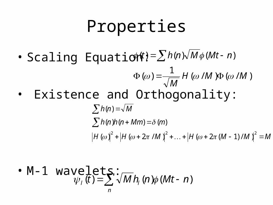
Properties

• Scaling Equation:

• Existence and Orthogonality:

• M-1 wavelets:

)/()/(1

)(

)()()(

MMHM

nMtMnht

MMMHMHH

mMmnhnh

Mnh

222)/)1(2()/2()(

)()()(

)(

)()()( nMtnhMt ln

l

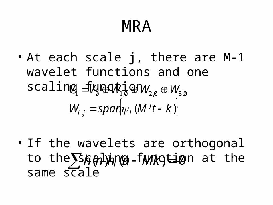
MRA

• At each scale j, there are M-1 wavelet functions and one scaling function

• If the wavelets are orthogonal to the scaling function at the same scale

)(,

0,30,20,101

ktMspanW

WWWVVj

ljl

0)()( Mknhnh l

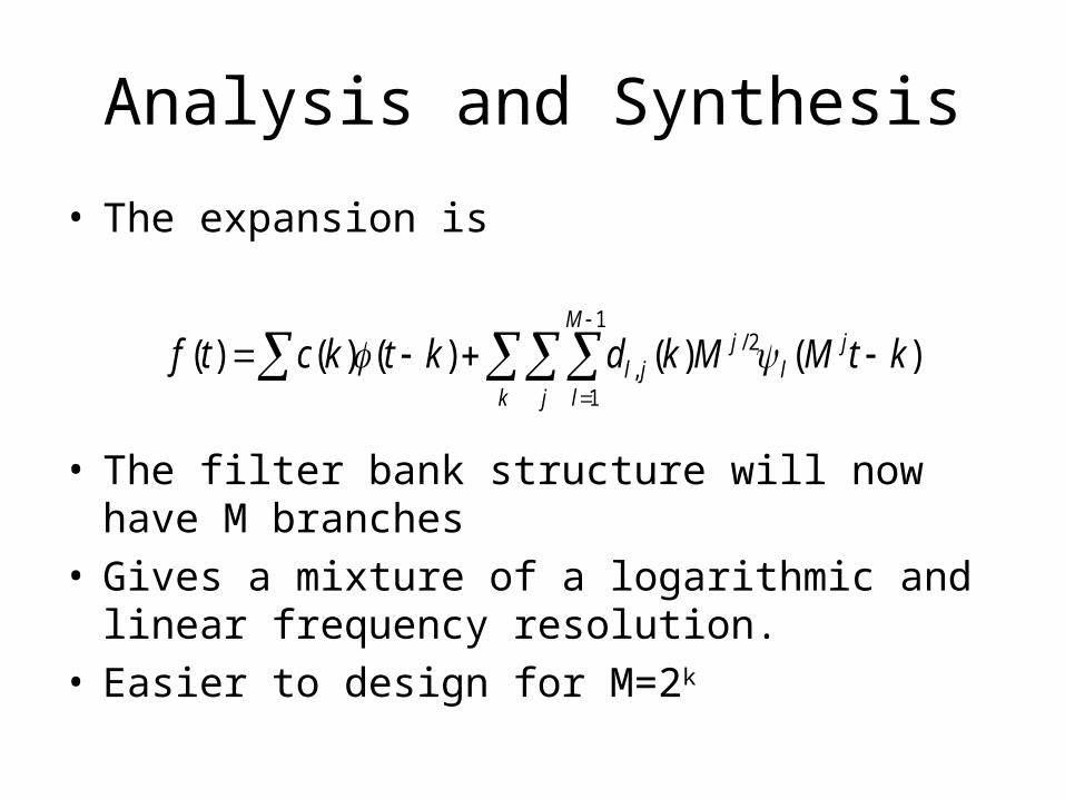
Analysis and Synthesis

• The expansion is

• The filter bank structure will now have M branches

• Gives a mixture of a logarithmic and linear frequency resolution.

• Easier to design for M=2k

)()()()()(1

1

2/, ktMMkdktkctf j

lk j

M

l

jjl

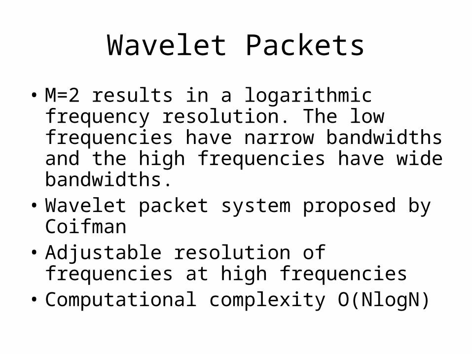
Wavelet Packets

• M=2 results in a logarithmic frequency resolution. The low frequencies have narrow bandwidths and the high frequencies have wide bandwidths.

• Wavelet packet system proposed by Coifman

• Adjustable resolution of frequencies at high frequencies

• Computational complexity O(NlogN)

Wavelet Packet Decomposition

• In order to have higher resolution decomposition at high frequencies, iterate the highpass wavelet branch

• Split both the lowpass and highpass bands at all stages• Evenly spaced frequency resolution• In DWT we consider the outputs of each channel.• In WPD, we have more outputs than inputs redundant

system• Choose an independent set as basis (not one unique

basis)

Optimization Criteria

• Search based on minimizing a cost function on the transform coefficients.

• Binary search algorithm for additive cost function• How do we choose the ‘best’ basis?

– Shannon entropy– Thresholding the coefficients– Log Energy– Norm of the coefficients

• Two approaches:– Choose a particular decomposition based on the signal class– Adapt the decomposition to each signal

Complexity

• P(J): The number of J-scale orthonormal wavelet packet transforms

• P(1)=1

• P(J)=P(J-1)2+1

• Application: FBI standard for fingerprint image compression

Haar Wavelet Packets

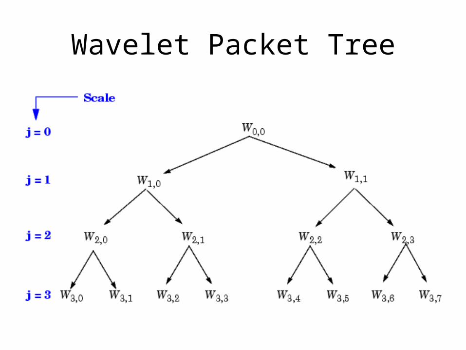
Wavelet Packet Tree

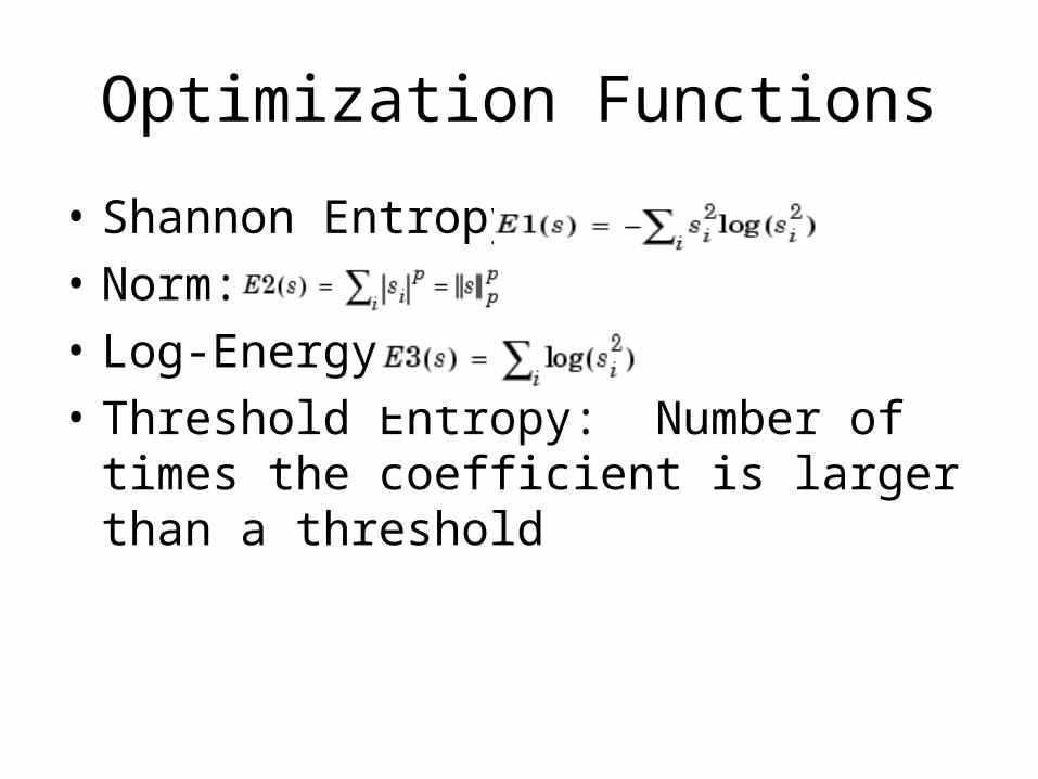
Optimization Functions

• Shannon Entropy:

• Norm:

• Log-Energy:

• Threshold Entropy: Number of times the coefficient is larger than a threshold

Example: Minimum Entropy Decomposition

• Start with a constant original signal. w00 = ones(1,16)*0.25; • Compute entropy of original signal.

– e00 = wentropy(w00,'shannon') e00 = 2.7726 • Then split w00 using the haar wavelet.

– [w10,w11] = dwt(w00,'db1'); • Compute entropy of approximation at level 1.

– e10 = wentropy(w10,'shannon') e10 = 2.0794 • The detail of level 1, w11, is zero; the entropy e11 is zero. Due to the additivity property the

entropy of decomposition is given by e10+e11=2.0794. This has to be compared to the initial entropy e00=2.7726. We have e10 + e11 < e00, so the splitting is interesting.

• Now split w10 (not w11 because the splitting of a null vector is without interest since the entropy is zero).

– [w20,w21] = dwt(w10,'db1'); • We have w20=0.5*ones(1,4) and w21 is zero. The entropy of the approximation level 2 is

– e20 = wentropy(w20,'shannon') e20 = 1.3863 • Again we have e20 + 0 < e10, so splitting makes the entropy decrease.• Then

– [w30,w31] = dwt(w20,'db1'); e30 = wentropy(w30,'shannon')     e30 = 0.6931 [w40,w41] = dwt(w30,'db1')     w40 = 1.0000     w41 = 0 e40 = wentropy(w40,'shannon')     e40 = 0

• Perform wavelet packets decomposition of the signal s.• t = wpdec(s,4,'haar','shannon');

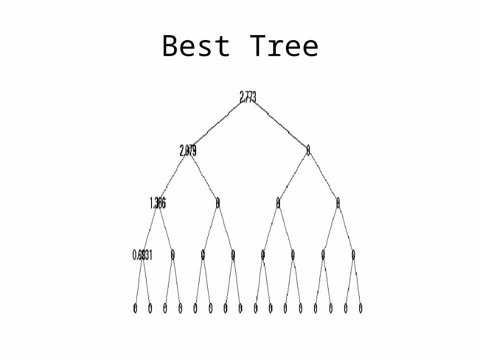
Best Tree

Overcomplete Representations, Frames, Redundant Transforms

• There are many cases where a single basis is not effective for signal representation.

• Example: Fourier basis is good for sinusoids, but bad for transients

• Efficiency of the transform can be improved by combining several basis systems.

• Combination of basis systemsOvercomplete• Collection of basis systems is called a dictionary.

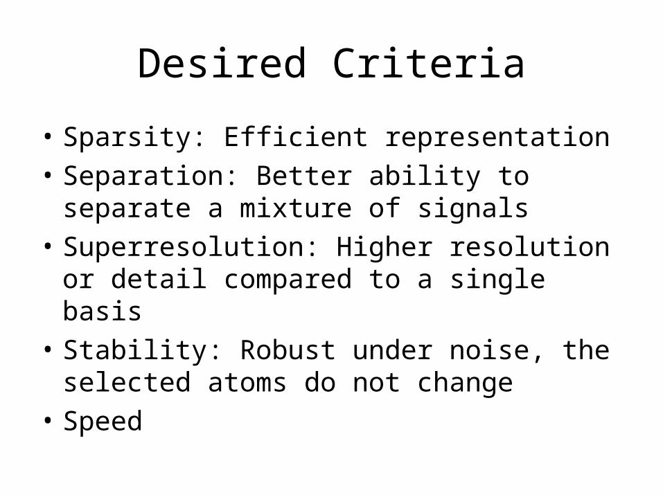
Desired Criteria

• Sparsity: Efficient representation

• Separation: Better ability to separate a mixture of signals

• Superresolution: Higher resolution or detail compared to a single basis

• Stability: Robust under noise, the selected atoms do not change

• Speed

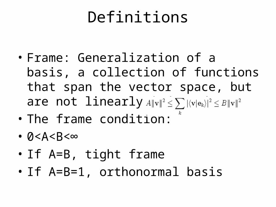
Definitions

• Frame: Generalization of a basis, a collection of functions that span the vector space, but are not linearly independent

• The frame condition:

• 0<A<B<∞

• If A=B, tight frame

• If A=B=1, orthonormal basis

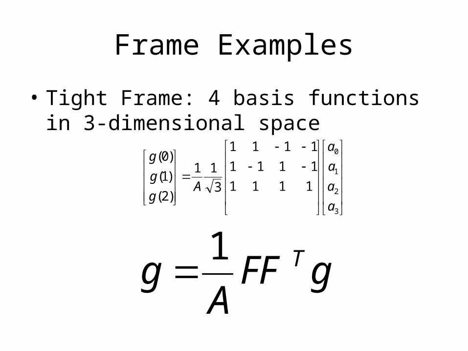
Frame Examples

• Tight Frame: 4 basis functions in 3-dimensional space

3

2

1

0

1111

1111

1111

3

11

)2(

)1(

)0(

a

a

a

a

Ag

g

g

gFFA

g T1

Matching Pursuit

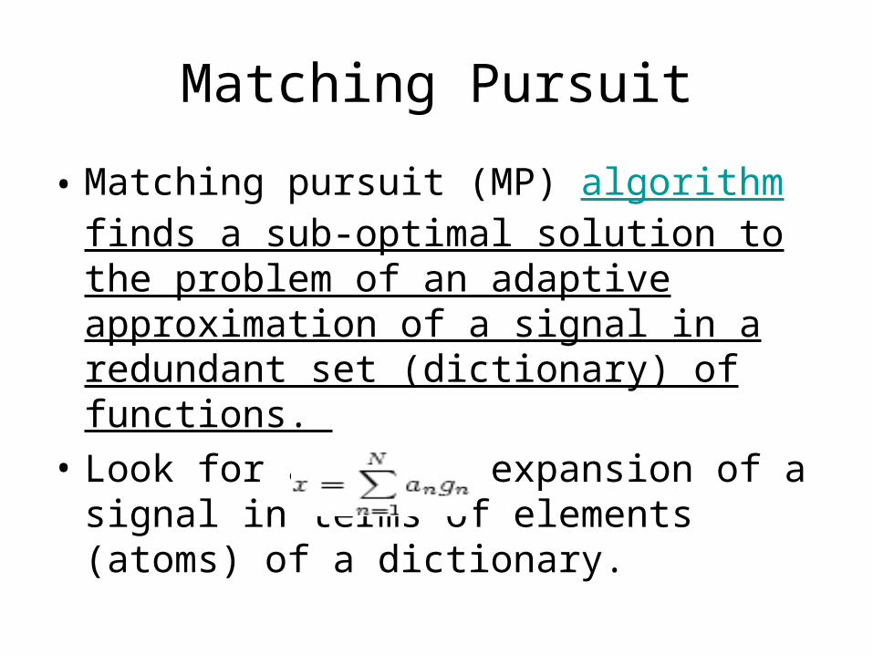
• Matching pursuit (MP) algorithm finds a sub-optimal solution to the problem of an adaptive approximation of a signal in a redundant set (dictionary) of functions.

• Look for a linear expansion of a signal in terms of elements (atoms) of a dictionary.

Algorithm [Mallat, Zhang 1993]

• At each step, try to find the element of the dictionary that ‘best’ fits the signal.

• Energy Conservation:• For a complete dictionary as M∞, the residue

should go to zero. • Stopping Criteria: Threshold the residue or pre-

determine M

Dictionary

• Commonly used dictionary: Gabor functions, dictionary of time-frequency atoms

• General and compact model for oscillations

• Compact time-frequency localization• Restrict the search to a range of time,

frequency, and scale values

Applications

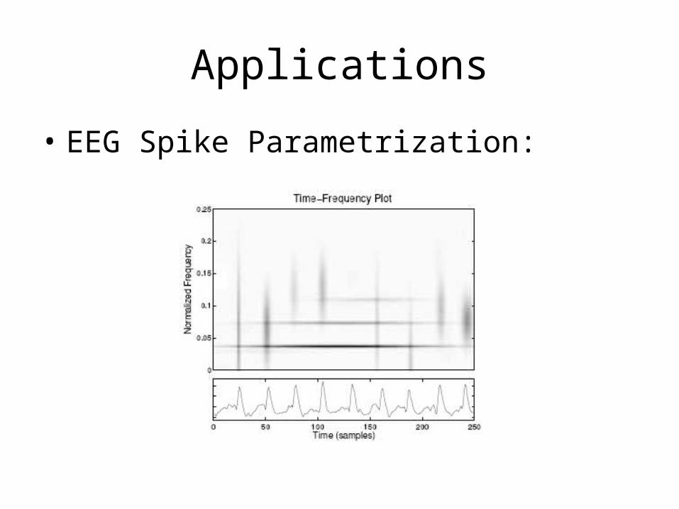
• EEG Spike Parametrization:

Extensions

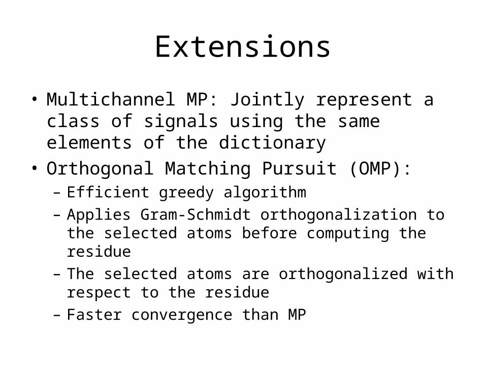
• Multichannel MP: Jointly represent a class of signals using the same elements of the dictionary

• Orthogonal Matching Pursuit (OMP):– Efficient greedy algorithm– Applies Gram-Schmidt orthogonalization to the

selected atoms before computing the residue– The selected atoms are orthogonalized with respect

to the residue– Faster convergence than MP

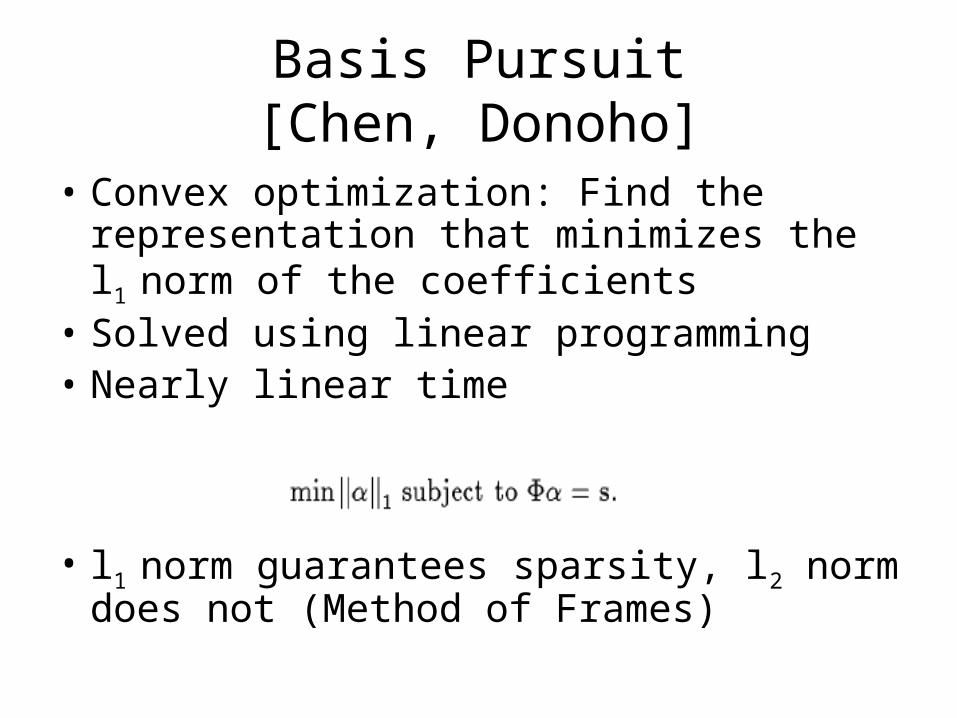
Basis Pursuit[Chen, Donoho]

• Convex optimization: Find the representation that minimizes the l1 norm of the coefficients

• Solved using linear programming• Nearly linear time

• l1 norm guarantees sparsity, l2 norm does not (Method of Frames)

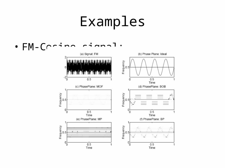
Examples

• FM-Cosine signal:

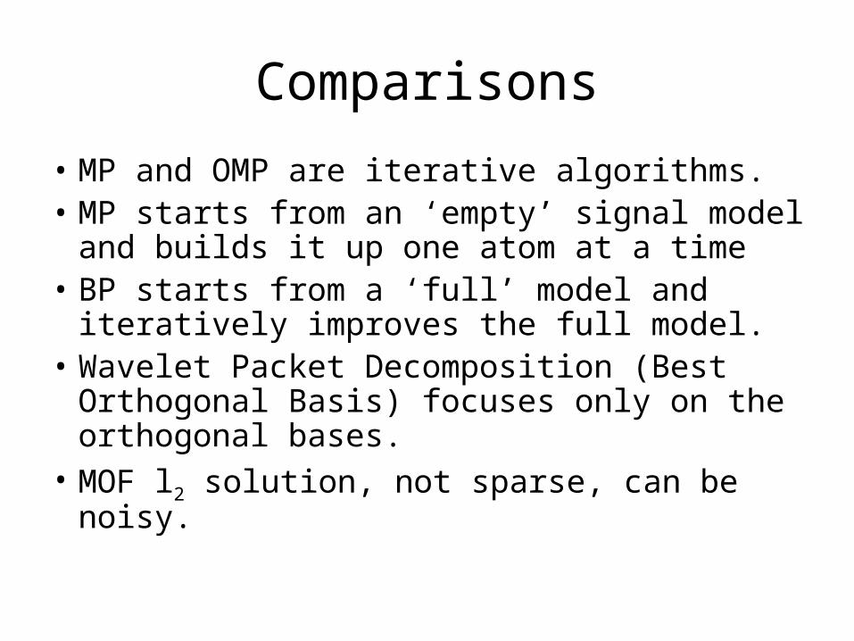
Comparisons

• MP and OMP are iterative algorithms.• MP starts from an ‘empty’ signal model

and builds it up one atom at a time• BP starts from a ‘full’ model and iteratively

improves the full model.• Wavelet Packet Decomposition (Best

Orthogonal Basis) focuses only on the orthogonal bases.

• MOF l2 solution, not sparse, can be noisy.