Embed Size (px)
Citation preview
Extensions to Consumer theory
Inter-temporal choiceUncertainty
Revealed preferences
Extensions to Consumer theory
We now know how a consumer chooses the most satisfying bundle out of the ones it can afford From observing changes in choice that follow
changes in price, we can derive the demand function.
But how useful (and realistic) is this theory? We assumed that agents have no savings... Does the theory still stand under uncertainty ? We assume that stable preferences just “exist”.
Extensions to Consumer theory
Inter-temporal choice
Uncertainty
Revealed preferences
Inter-temporal choice
The typical agents spreads his consumption over several periods of time: immediate consumption, savings, borrowing, etc.
Consume today / consume tomorrow Current preferences between goods are convex. Seems this is also the case for inter-temporal choices
We need to define : Inter-temporal preferences Inter-temporal budget constraint
Inter-temporal preferences
Preference for current consumption A unit of consumption today is “worth” more than a
unit of consumption tomorrow I’d rather receive 100 € today than 100 € next week !
If I give up some current consumption , I expect to receive a return (r) in compensation.
There must exist a value of (r), a psychological interest rate, for which I am indifferent between current and future consumption Would you rather receive 100 € today or 101 € next
week ? What about 120 € ?
Inter-temporal preferences
future consumption
(c2)
current consumption (c1)
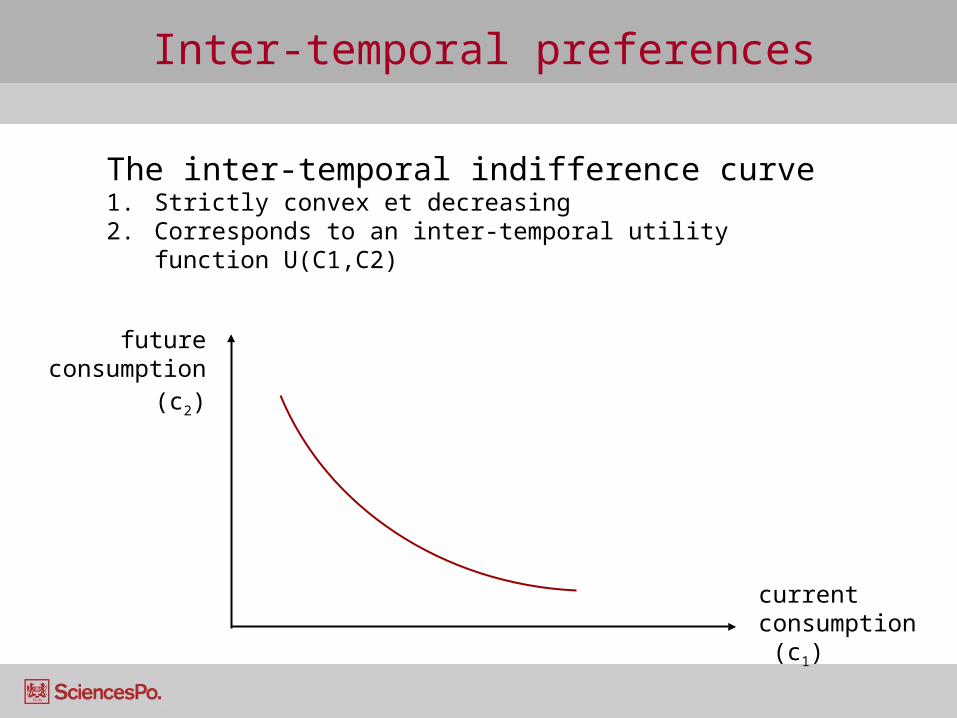
The inter-temporal indifference curve1. Strictly convex et decreasing 2. Corresponds to an inter-temporal utility function
U(C1,C2)
Inter-temporal preferences
A
2
1
1 a
cr
c
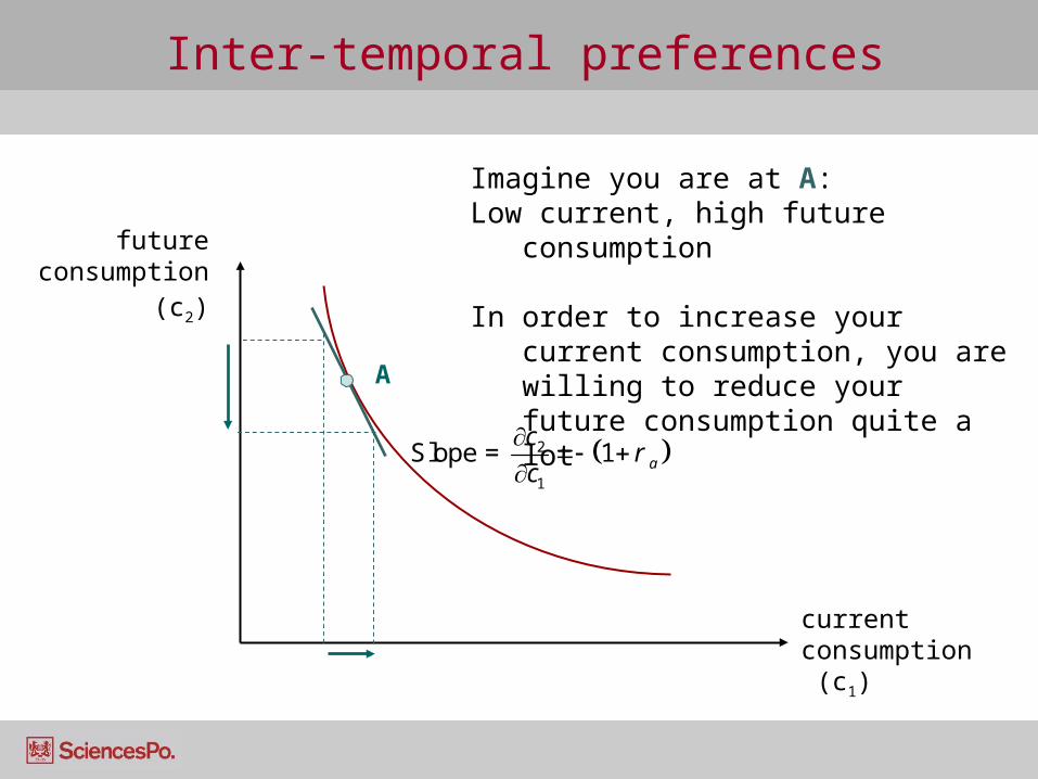
Slope =
Imagine you are at A:Low current, high future
consumption
In order to increase your current consumption, you are willing to reduce your future consumption quite a lot
future consumption
(c2)
current consumption (c1)
Inter-temporal preferences
A
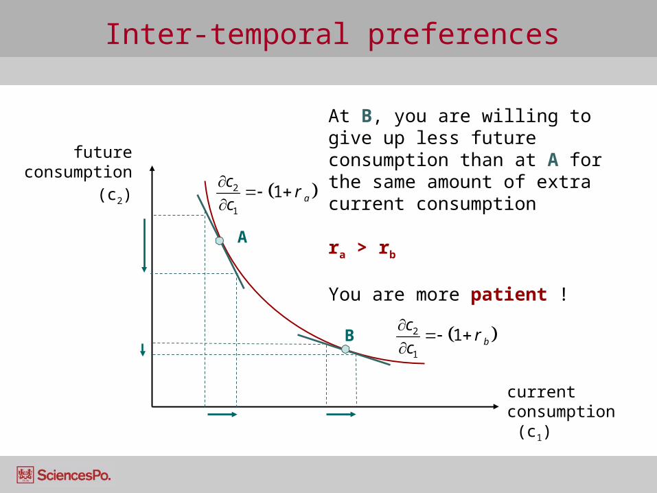
At B, you are willing to give up less future consumption than at A for the same amount of extra current consumption
ra > rb
You are more patient !
B
future consumption
(c2)
current consumption (c1)
2
1
1 b
cr
c
2
1
1 a
cr
c
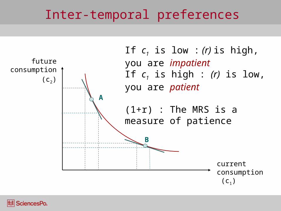
Inter-temporal preferences
A
B
If c1 is low : (r) is high, you are impatientIf c1 is high : (r) is low, you are patient
(1+r) : The MRS is a measure of patience
future consumption
(c2)
current consumption (c1)
Inter-temporal budget constraint
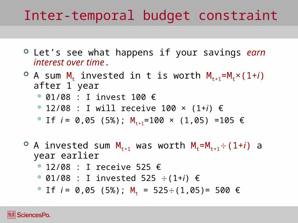
Let’s see what happens if your savings earn interest over time.
A sum Mt invested in t is worth Mt+1=Mt×(1+i) after 1 year 01/08 : I invest 100 € 12/08 : I will receive 100 × (1+i) € If i = 0,05 (5%); Mt+1=100 × (1,05) =105 €
A invested sum Mt+1 was worth Mt=Mt+1(1+i) a year earlier 12/08 : I receive 525 € 01/08 : I invested 525 (1+i) € If i = 0,05 (5%); Mt = 525(1,05)= 500 €
Inter-temporal budget constraint
Simplification: invariable price p1 = p2 = 1 Explicit interest rate: i Consumption : c Budget : b Two periods : 1 and 2
Inter-temporal budget constraint
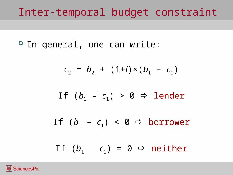
In general, one can write:
c2 = b2 + (1+i)×(b1 – c1)
If (b1 – c1) > 0 lender
If (b1 – c1) < 0 borrower
If (b1 – c1) = 0 neither
Inter-temporal budget constraint
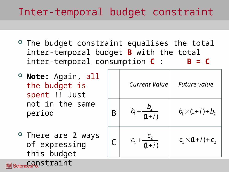
Current Value Future value
B
C
21 (1 )
bb
i
21 (1 )
cc
i
1 2(1 )b i b
1 2(1 )c i c
The budget constraint equalises the total inter-temporal budget B with the total inter-temporal consumption C : B = C
Note: Again, all the budget is spent !! Just not in the same period
There are 2 ways of expressing this budget constraint
Inter-temporal budget constraint
2 21 1
2 1 2 1
1 1
1 1
b cb c
i i
b i b c i c
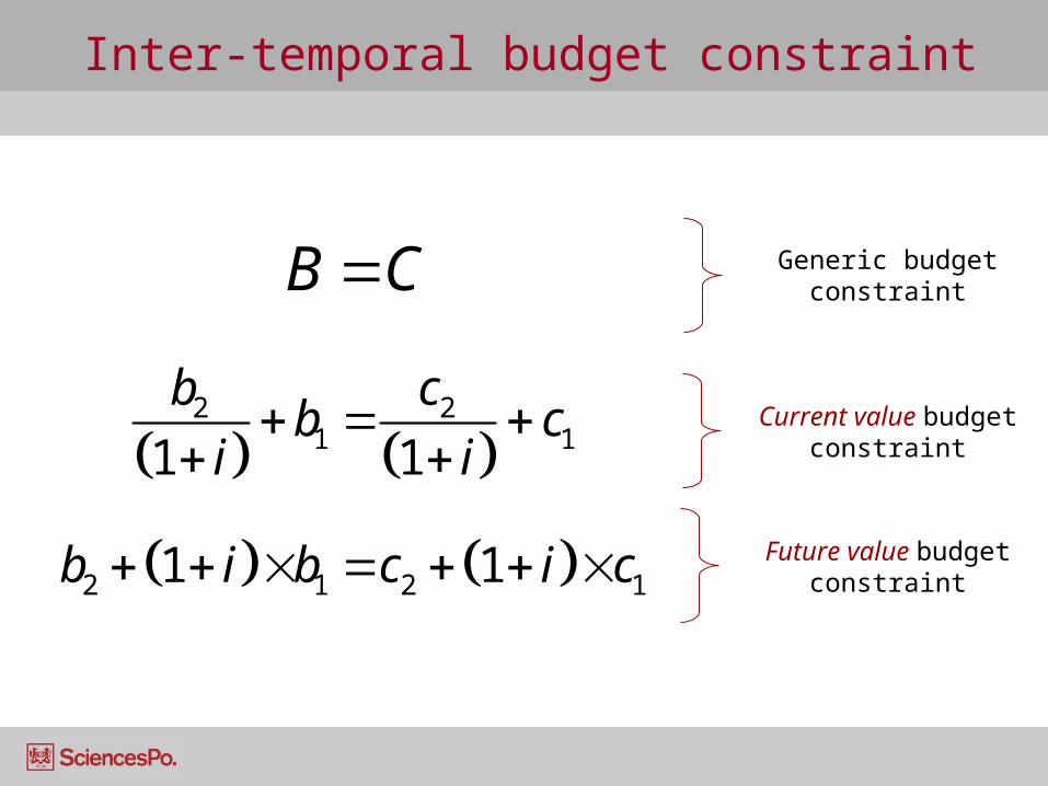
Current value budget constraint
Future value budget constraint
Generic budget constraintB C
Inter-temporal budget constraint
2 12
1B
b i bp
2
11 1
bBb
p i
2
1
1c
ic
Slope =
future consumption
(c2)
current consumption (c1)
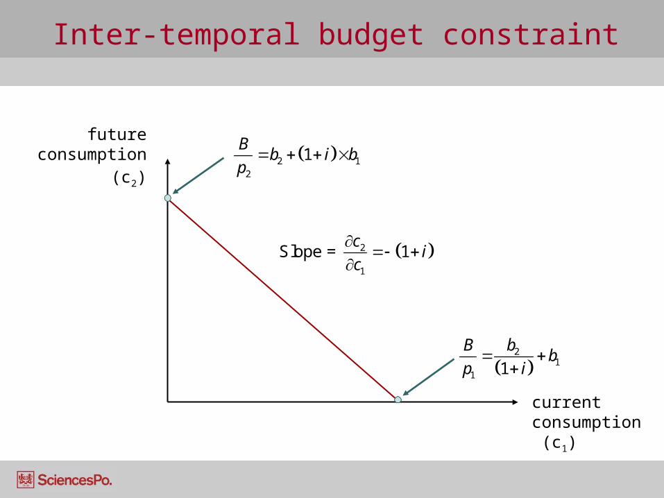
Inter-temporal budget constraint
2
11
bb
i
2 1 1b b i
A
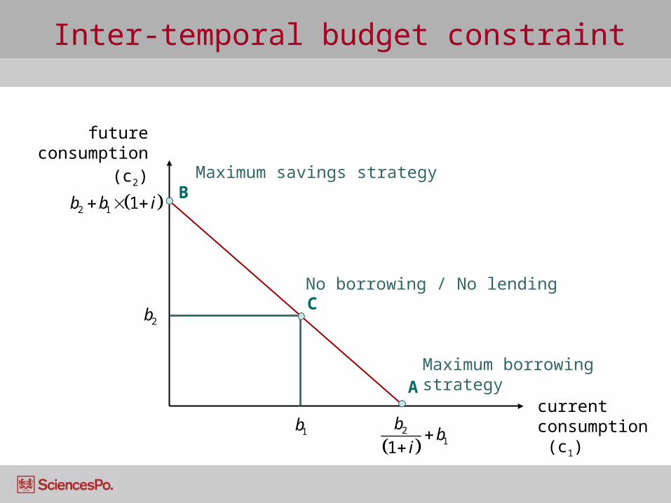
B
1b
2bC
Maximum savings strategy
Maximum borrowing strategy
No borrowing / No lending
future consumption
(c2)
current consumption (c1)
Inter-temporal budget constraint
2
11
bb
i
2 1 1b b i
A
B
1b
2bC
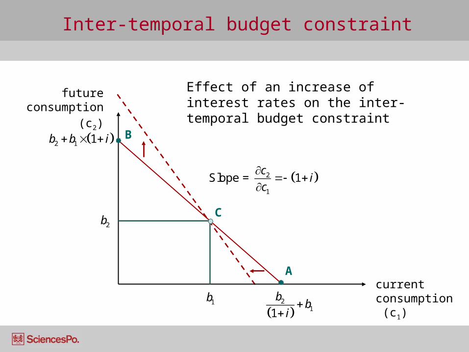
future consumption
(c2)
current consumption (c1)
Effect of an increase of interest rates on the inter-temporal budget constraint
2
1
1c
ic
Slope =
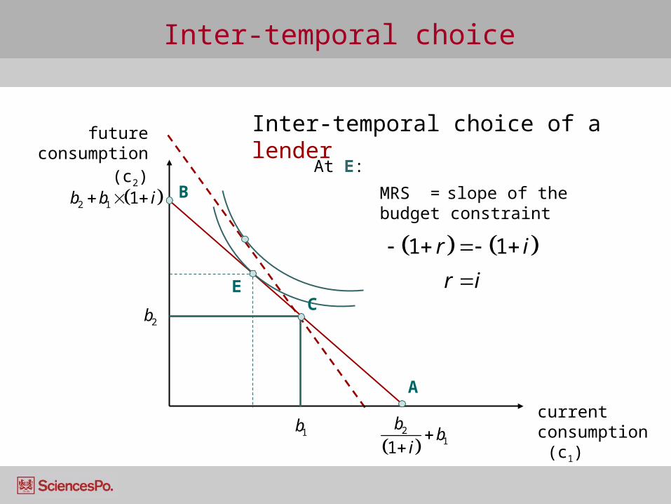
Inter-temporal choice
2
11
bb
i
2 1 1b b i
A
B
E
Inter-temporal choice of a lenderfuture consumption
(c2)
current consumption (c1)
1b
2bC
At E:
1 1r i
r i
MRS = slope of the budget constraint
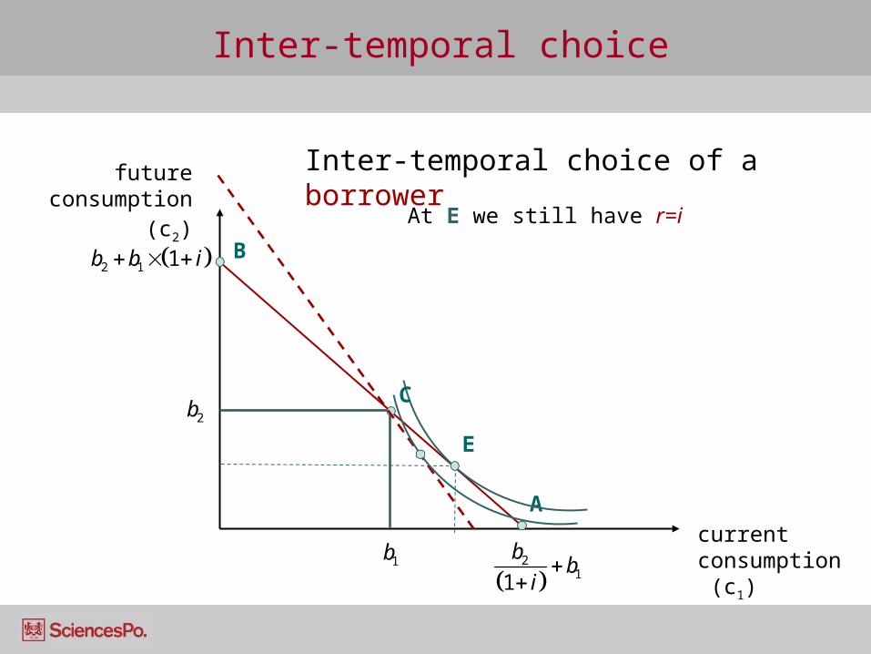
Inter-temporal choice
2
11
bb
i
2 1 1b b i
A
B
E
Inter-temporal choice of a borrower
1b
2bC
future consumption
(c2)
current consumption (c1)
At E we still have r=i
Extensions to Consumer theory
Inter-temporal choice
Uncertainty
Revealed preferences
Uncertainty
How do we calculate the utility of an agent when there is uncertainty about which bundle will be consumed?
Example: You’re trying to decide if you want to buy a raffle ticket. What determines the potential utility of buying this ticket? The amount of prizes and their value The amount on tickets on sale
Uncertainty
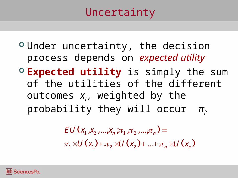
Under uncertainty, the decision process depends on expected utility
Expected utility is simply the sum of the utilities of the different outcomes xi, weighted by the probability they will occur πi.
1 2 1 2
1 1 2 2
, ,..., ; , ,...,
...
n n
n n
EU x x x
U x U x U x
Uncertainty
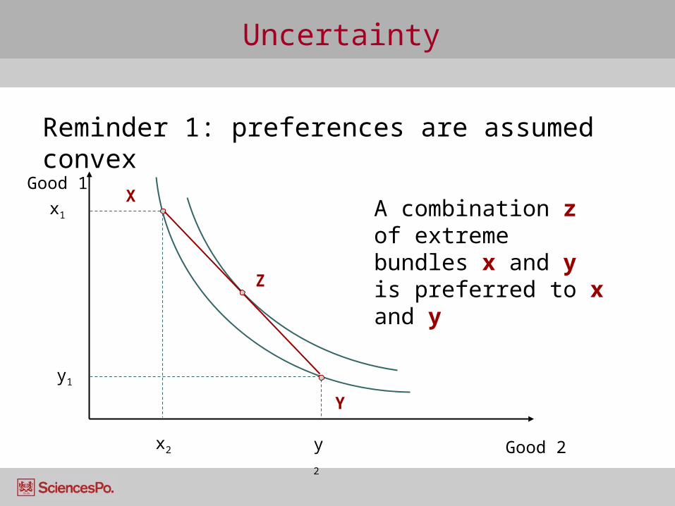
Reminder 1: preferences are assumed convex
Good 1
Good 2
y1
y2
Y
x1
x2
XA combination z of extreme bundles x and y is preferred to x and yZ
Uncertainty
Good
Utility
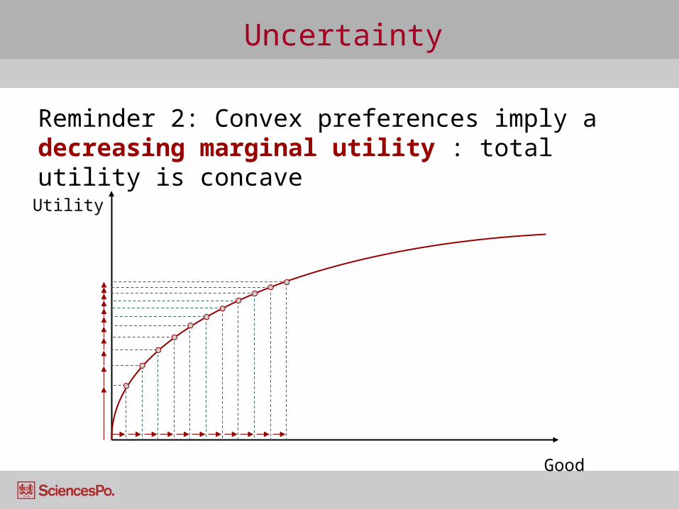
Reminder 2: Convex preferences imply a decreasing marginal utility : total utility is concave
Uncertainty
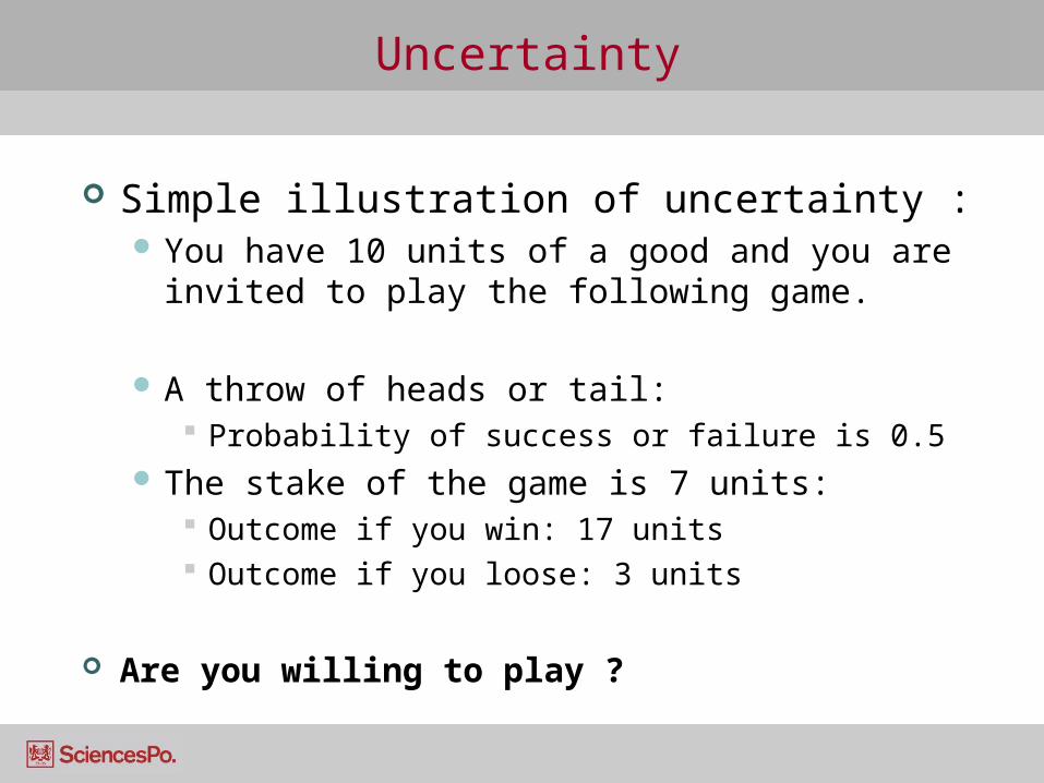
Simple illustration of uncertainty : You have 10 units of a good and you are invited
to play the following game.
A throw of heads or tail: Probability of success or failure is 0.5
The stake of the game is 7 units: Outcome if you win: 17 units Outcome if you loose: 3 units
Are you willing to play ?
Uncertainty
Good
Utility
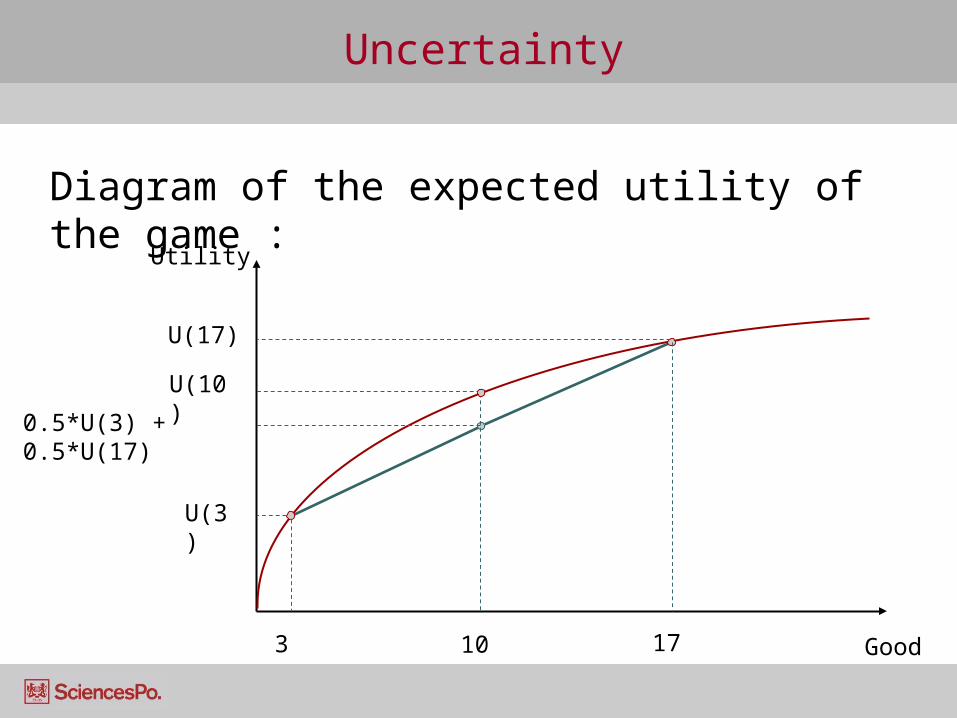
Diagram of the expected utility of the game :
3
U(3)
10
U(10)
17
U(17)
0.5*U(3) + 0.5*U(17)
Uncertainty
In this example, the expected result does not change the expected endowment of the agent.The player starts with 10 units and the net
expected gain is 0.
Even though the expected outcome is the same as the initial situation, the mere existence of the game reduces the utility of the agent.
Why is that ?
Uncertainty
Good
Utility
3
U(3)
10
U(10)
17
U(17)
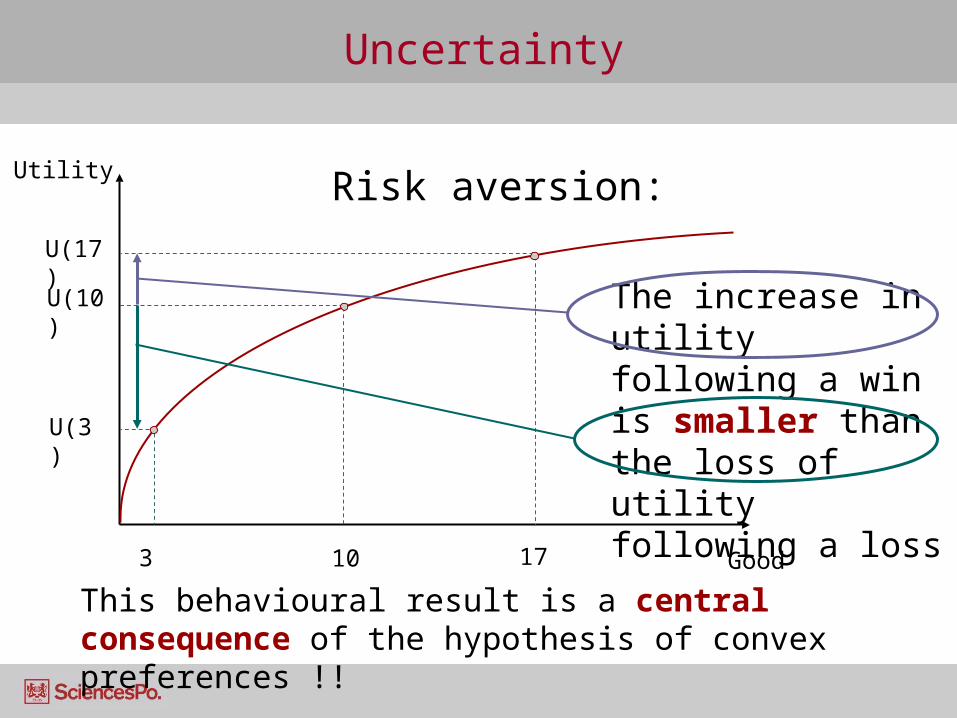
The increase in utility following a win is smaller than the loss of utility following a loss
This behavioural result is a central consequence of the hypothesis of convex preferences !!
Risk aversion:
Uncertainty
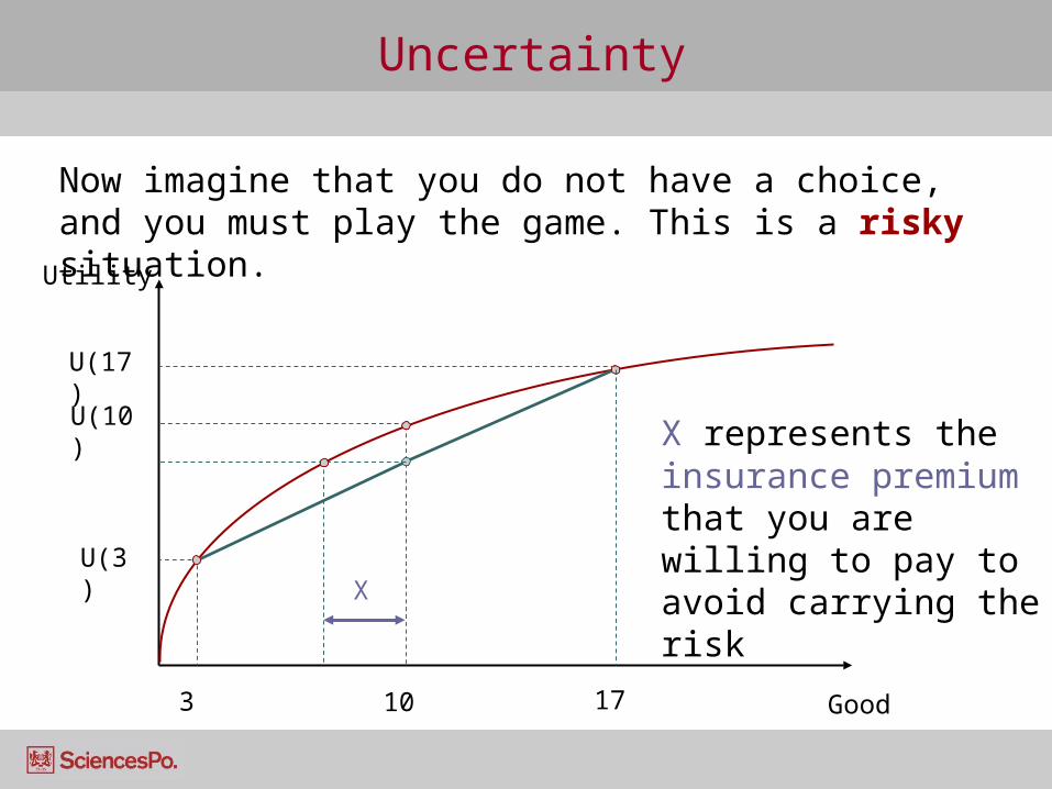
Now imagine that you do not have a choice, and you must play the game. This is a risky situation.
Good
Utility
3
U(3)
10
U(10)
17
U(17)
X represents the insurance premium that you are willing to pay to avoid carrying the riskX
Adapting to Uncertainty/risk
Insurance: Agents are willing to accept a smaller endowment to mitigate
the presence of risk A risky outcome, however, does not impact all agents.
Insurance spreads this risk over all the agents: This is known as the mutualisation of risk.
Diversification behaviour: Imagine you sell umbrellas: your income depends on the
weather, so your future income is uncertain. How can you make your income more certain? Sell some ice-
creams on the side !! Financial markets:
Spread the risk over many assets instead of concentrating it on a few.
You can “sell” your risk to agents that are willing to carry it, against a payment. But beware of information problems !!
Extensions to Consumer theory
Inter-temporal choice
Uncertainty
Revealed preferences
Revealed preferences
Up until now we have assumed that preferences and indifference curves are given, and are stable This assumption was required for the purpose of
developing a theory of choice ! But we’ve never directly observed them. How do
we know we’re right?
We can reverse the theory: we work backwards from the optimal bundle and the budget constraint to get to the indifference curve.
Past choices/decisions reveal your preferences
Revealed preferences
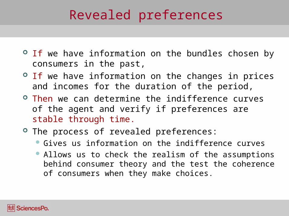
If we have information on the bundles chosen by consumers in the past,
If we have information on the changes in prices and incomes for the duration of the period,
Then we can determine the indifference curves of the agent and verify if preferences are stable through time.
The process of revealed preferences: Gives us information on the indifference curves Allows us to check the realism of the assumptions
behind consumer theory and the test the coherence of consumers when they make choices.
Revealed preferences
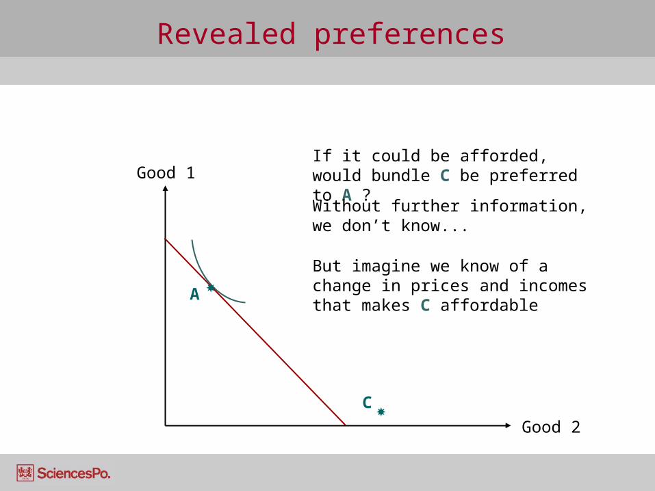
A
If it could be afforded, would bundle C be preferred to A ?
C
Good 1
Good 2
Without further information, we don’t know...
But imagine we know of a change in prices and incomes that makes C affordable
Revealed preferences
Good 2
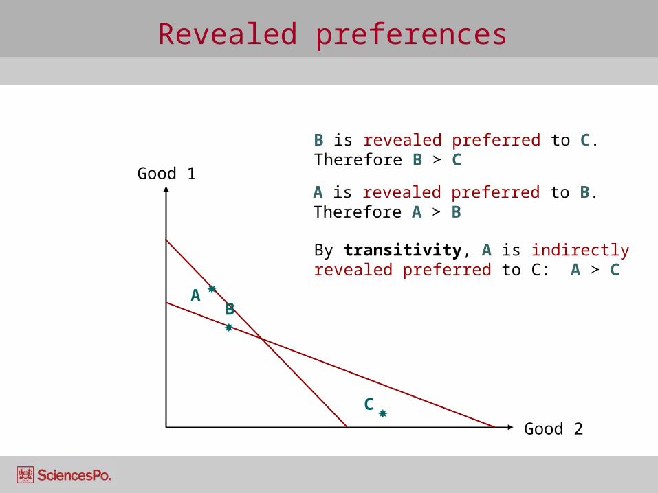
B is revealed preferred to C. Therefore B ≻ C
C
A is revealed preferred to B. Therefore A ≻ B
By transitivity, A is indirectly revealed preferred to C: A ≻ C
B
Good 1
A
Revealed preferences
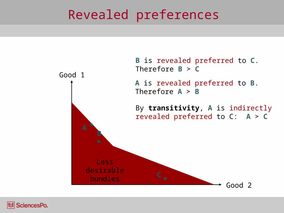
Less desirable bundles
Good 1
Good 2
C
B
A
B is revealed preferred to C. Therefore B ≻ C
A is revealed preferred to B. Therefore A ≻ B
By transitivity, A is indirectly revealed preferred to C: A ≻ C
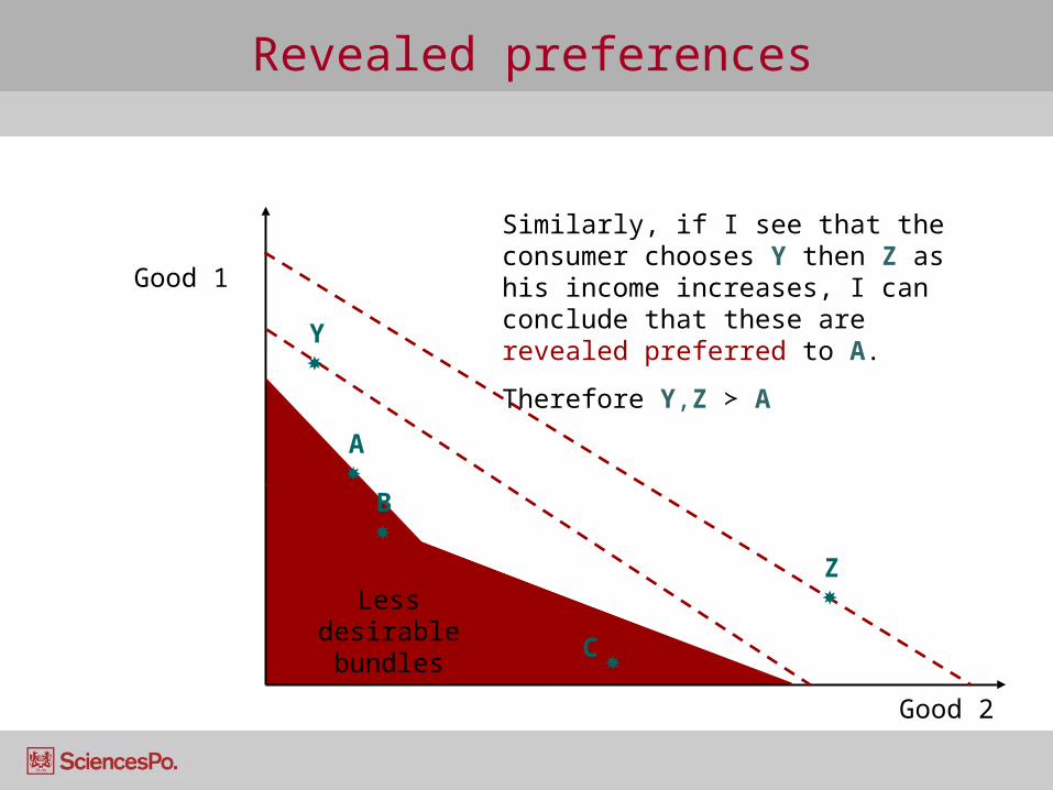
Revealed preferences
Good 1
Good 2
C
A
B
Y
Z
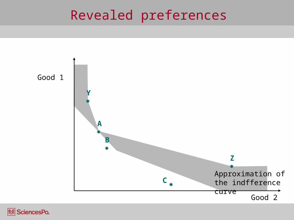
Similarly, if I see that the consumer chooses Y then Z as his income increases, I can conclude that these are revealed preferred to A.
Therefore Y,Z ≻ A
Less desirable bundles
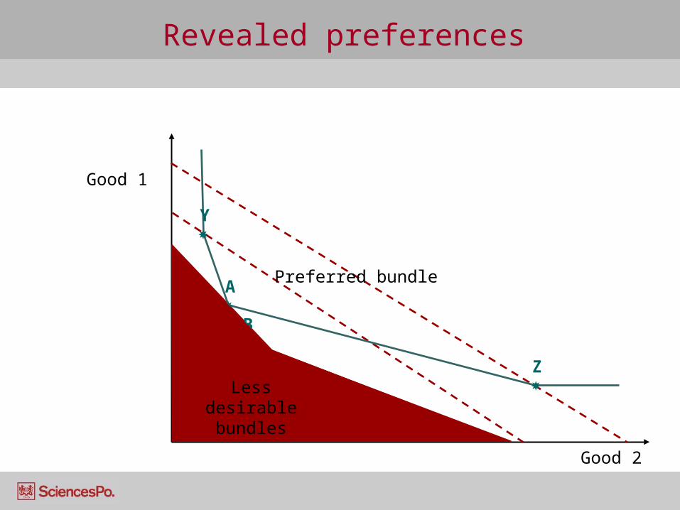
Revealed preferences
Good 2
C
A
B
Y
Z
Preferred bundle
Good 1
Less desirable bundles
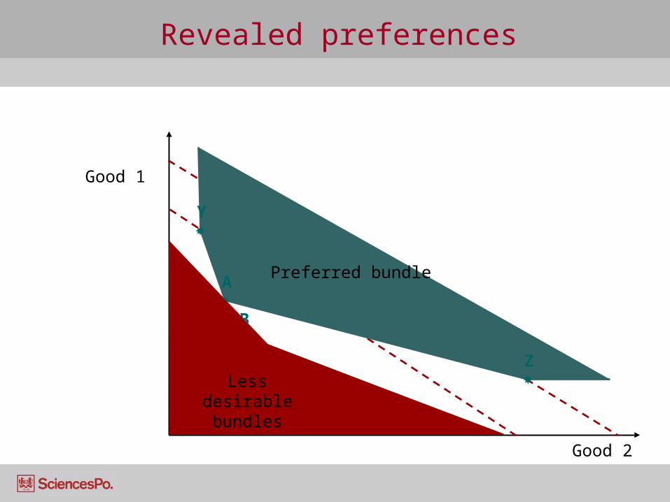
Revealed preferences
Good 2
C
A
B
Y
Z
Good 1
Preferred bundle
Less desirable bundles
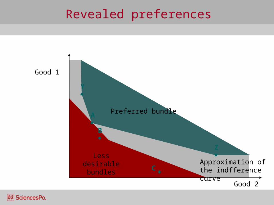
Revealed preferences
Good 2
C
A
B
Y
Z
Preferred bundle
Approximation of the indfference curve
Good 1
Less desirable bundles
Revealed preferences
Good 2
C
A
B
Y
Z
Approximation of the indfference curve
Good 1

Revealed preferences
Good 2
C
A
B
Y
Z
Approximation of the indfference curve
Good 1