Embed Size (px)
Citation preview
External Wars, Internal Conflict and State Capacity:
Panel Date Evidence
Mauricio Cárdenas, Marcela Eslava, Santiago Ramírez
1
EXTERNAL WARS, INTERNAL CONFLICT AND STATE CAPACITY:
PANEL DATA EVIDENCE1
Mauricio Cárdenas2
Marcela Eslava3
Santiago Ramírez4
ABSTRACT
Relying on cross-country data, empirical studies have pointed at external wars as
engines for the development of a state’s capacity, and at internal conflicts as having
the opposite effect. Concerns about possible reverse causality driving these results
emerge, as the cross-sectional approach ignores the role of initial conditions and the
persistence of state capacity. This paper re-examines the impact of external and
internal conflict on state capacity using panel data to overcome these limitations.
Two different data panels are analyzed, one covering countries, another covering
Colombian municipalities. Beyond methodological differences with respect to
previous work, we also add to the existing literature by looking at the impact of
different attributes of conflicts: intensity, and types of conflict-related events. Large
variability across municipalities allows us to zoom on multiple dimensions of
conflict. We find that internal conflicts deteriorate state capacity both at the country
and municipal level, and that more intense conflicts have a stronger negative
impact. Moreover, episodes where civilians feel targeted affect the state’s capacity
to collect taxes, while those with more general reach affect the state’s capacity to
provide public goods. External conflicts, however, do not seem to affect on state
capacity once initial conditions and endogeneity issues are taken into account.
1 We thank participants at the 2010 AEA meetings and the 2010 LACEA Annual Meeting for very helpful
comments. Andrés Corredor assisted with the municipal database and José Tessada provided crucial country
data. 2 Senior Fellow, Brookings Institution. Email: [email protected]
3 Associate Professor of Economics, Universidad de los Andes. Email: [email protected]
4 Graduate student, Universidad de Los Andes. Email: [email protected]
2
1. INTRODUCTION
Despite its pedigree in various social sciences, state capacity is a relatively unknown
concept in the economics literature in part because it is complex to define and measure.
There are many interpretations in the political science and sociology literatures. In these
contexts, state capacity is associated to military capacity, representing the state’s ability to
overcome rebellious actions with force, or to bureaucratic and administrative capacity,
representing the ability of the state to conduct its business effectively and efficiently.
A recent interest for state capacity has emerged in economics. In the recent
economics literature, a distinction is often made between ―legal‖ and ―fiscal‖ state capacity.
Legal capacity refers to issues such as the availability of ―contracting institutions‖ (i.e.,
institutions supporting private contracts) and ―property rights institutions‖ (i.e., institutions
constraining government expropriation), to use the terminology in Acemoglu and Johnson
(2005). Fiscal state capacity deals with questions such as the ability to raise revenue from
the society --typically measured by the GDP share of total taxes—and has been the focus of
a number of contributions, including the forthcoming book by Besley and Persson (2011).
On the specific question of the relationship between conflict and state capacity,
according to the ―bellicist‖ approach to state building it is wars that make states. Military
confrontations require increases in the level of taxation (the so-called ratchet effect) and
demand greater state capacity. Fearing external domination, a consensus emerges around
the idea of strengthening the state by increasing taxation. In this sense, wars are a rare
moment of national unity, which is essential to build states. The work of Tilly (1990),
among many others, reaches this conclusion based on the experiences of the U.S. and
Western Europe. In fact, modern history is rich in examples of the association between
wars and the introduction and development of the modern income tax systems. More
broadly, Stubbs (1999) claims that war (or the threat of) has been an important factor in
molding state institutions in the most successful economies of East Asia (namely, Japan,
South Korea, Hong Kong, Malaysia, Singapore, Taiwan, and Thailand), while Desch
(1996) looks into the cases of China, Cuba, Israel, and South Korea to conclude that their
threatening external environments have resulted in stronger states.
3
Centeno (1997 and 2002) and López-Alves (2000) have explored the role of wars in
state formation in Latin America. A major insight in their contributions is that external and
internal wars are two distinct types of conflict with potentially opposing effects in the
development of state capacity. While external wars are moments of unity and consensus,
which facilitate the decision to invest in state capacity, internal wars are by definition
divisive and destructive. The testable implication of this proposition is that external and
internal have opposite effects on state capacity. In recent work, Besley and Persson (2008,
2009) provide empirical evidence that supports this view. Using cross-sectional data they
show that the incidence of external wars is associated with stronger states, while the
incidence of internal wars goes in the opposite direction.
These conclusions have been reached using cross-sectional data which has
important limitations. Specifically, one of the main features of state capacity is that it
persists over time, much like other institutional measures. This means that present state
capacity is highly correlated with past state capacity. In addition, past state capacity may
have been an important driver of a country’s decision to engage in previous conflicts:
stronger states may be more likely to fight wars with other states, while internal groups may
be more likely to challenge the state if it is weak. This implies that ignoring the persistent
nature of state capacity could lead to biased estimates of the effects of earlier conflicts. In
other words, concerns about reverse causality arise when the effects of past state capacity
are not properly acknowledged in econometric specifications. The nature of the cross-
sectional data used in earlier work is such that earlier measures of state capacity cannot be
taken into account, and so addressing these concerns requires a different empirical strategy.
The goal of this paper is to re-examine the impact of external and internal conflict
on state capacity using panel data to overcome the above-mentioned limitations. Two
different sets of data are analyzed: a panel covering cross-country information, and a panel
of Colombian municipalities. The availability of panel data enables us to control for the
persistence of state capacity and country fixed effects (including initial conditions), and use
dynamic panel GMM estimation techniques to address concerns about the endogeneity of
both conflict and other determinants of state capacity. This methodological approach also
allows us to control for the level of development and other determinants of state capacity
4
that are not included in cross-sectional regressions due to concerns about them responding
endogenously to state capacity.
Beyond these differences with respect to previous work, our analysis also
contributes by examining how different types of conflicts affect state capacity. In particular,
we analyze the effects of different levels of conflict intensity (measured in terms of
numbers of casualties). We also take advantage of heterogeneity across Colombian
municipalities in terms of conflict-related events to assess their differential impact on state
capacity. One limitation of our databases is that they cover only a recent period, so we are
unable to identify effects of conflict that may take place over the long horizons (which is
the emphasis of the cross-sectional work mentioned above). However, if conflicts affect the
incentives to invest in state capacity, then such relationship should show up in the data even
in short horizons. Otherwise, the benefits of those investments would only be realized long
after the war is over, calling into question the hypothesis that the capacity of the state was
made stronger precisely to fight the conflict. Our results show that internal conflicts
deteriorate state capacity both at the cross-country and within-country levels, and that more
intense conflicts have a stronger negative impact. External conflicts, however, do not seem
to have a clear effect on state capacity, once initial conditions and endogeneity issues are
taken into account. We also find that some types of conflict-related events are negatively
correlated with state capacity across Colombian municipalities. In particular, conflict
manifestations that affect targeted civilians affect the state’s capacity to collect taxes, while
those with more general reach affect the state’s capacity to provide public goods.
The paper is structured as follows. The next section presents the evidence related to
the panel of countries. It starts by revisiting previous results, using standard cross-country
OLS regressions, and then moves on to the dynamic estimations based on a GMM
procedure. The following section focuses on the issue of internal conflict by using the panel
of municipalities from Colombia. The final section provides a conclusion.

5
2. CROSS-COUNTRY EVIDENCE: THE PANEL DIMENSION
We begin by examining the relationship between the incidence of conflicts and state
capacity for a panel of country-year observations covering the period 1975-2004. We first
present the data, and then move on to the detailed empirical strategy and results.
Data
Our state capacity measures for the panel of countries relate to the fiscal and legal
dimensions discussed above: we measure fiscal capacity with total tax revenue as a
percentage of GDP and income tax revenue as a percentage of GDP (following Besley and
Persson, 2009). Data on these variables comes from Baunsgaard and Keen (2010), who take
total tax revenue data from the IMF’s Government Financial Statistics (GFS) between 1975
and 2006 and improve it for countries outside the OECD. They do this with revenue
information provided in the context of the IMF’s periodic consultations with member
countries, thus making the data more reliable.5 We measure legal capacity through a
summary indicator of the quality of government reported by the Quality of Government
Institute (QOG), based on the International Country Risk Guide (ICRG).6 This measure
averages individual scores for three dimensions: law and order, corruption, and quality of
bureaucracy. It takes values between zero and one, and increases with the assessed quality
of government.7 This variable is available for the period 1984-2008.
Turning to the explanatory variables, we use various measures of conflict from the
UCDP/PRIO Armed Conflict Dataset (version 3-2005), also available in the QOG panel
database. The data provides information on armed conflicts for the period 1946-2004. It
records all armed conflicts following the definitions of the Uppsala Conflict Data Program
5 Data for income tax as a percentage of GDP is only available until 2000.
6 The Quality of Government Dataset (QOG) from the QOG Institute at the University of Gothenburg
compiles annual information for the period 1946–2008. The datasets can be freely downloaded at
http://www.qog.pol.gu.se/. For details see Teorell et al. (2009). Matching the country classifications between
the different data sources we use requires additional assumptions that are explained in the appendix. We use
current countries only but to get historical data in cases of unification (division) we use the absorbing
(original) country. 7 The QOG measure is similar to the one constructed by Knack and Keefer (1995), and later used by Hall and
Jones (1999), to quantify the quality of government. Knack and Keefer (1995) average 5 of the original 24
categories created by the ICRG to rank countries. These five categories are "law and order," "bureaucracy
quality," "corruption," "risk of expropriation" and "government repudiation of contracts." QOG only uses the
first three in its indicator of the quality of government because the latter two were discontinued in 1997.
6
(UCDP) at the Department of Peace and Conflict Research, Uppsala University, and the
Centre for the Study of Civil War at the International Peace Research Institute in Oslo,
Norway (PRIO). Conflicts are defined as such when there are at least 1,000 battle-related
deaths over the full span of the episode. Internal conflicts are those that occur between the
government of a state and internal opposition groups, without intervention from other
states. External conflicts, meanwhile, are defined as those that occur between two or more
states.8
Our control variables are year effects, real GDP per capita and a measure of
democracy. Our dependent variables (in particular the fiscal ones) can be affected by global
phenomena, such as economic crises, controlled for by the inclusion of year effects.
Moreover, tax collections plausibly depend on income levels. (More generally, state
capacity is a function of a country’s level of development; we believe this statement applies
more in the long run than for within-country variability, and in that sense country fixed
effects should be the main way in which some of our regressions capture this specific
mechanism). It has also been shown that inclusive political institutions are central to
building state capacity (Besley and Persson, 2009; Cárdenas and Tuzemen, 2010). Country
effects and lagged dependent variables are added in some of the specifications, in particular
our preferred ones.
Real GDP per capita data comes from the QOG database, which in turn takes the
information from Gleditch (2002).9 As for democracy, we use a revised version of the
Combined Polity Score from the Polity IV Project, named Polity2 (Marshall et al., 2009),
which ranges from -10 (complete autocracy) to +10 (complete democracy). The index of
democracy we use in our regressions is a dummy variable that takes the value of 1 if the
Polity2 score, averaged over the five preceding years, is above 3.10
Table 1 reports descriptive statistics for our panel of countries. The sample covers
188 countries, with 140 of them having information on all variables, over 1975-2004. It is
8 We use the UCDP/PRIO conflict dataset as opposed to the more conventional Correlates of War Dataset
(COW) because it provides data up to 2004 while the latter only does so until 1997. 9 Gleditsch (2002) fills gaps in the original data of the Penn World Tables using additional sources and
extrapolation techniques. 10
Results are robust to using a cutoff of zero rather than three.
7
worth noting that internal conflicts are much more frequent than external conflicts. In our
sample of countries and years, 11 percent of the observations correspond to internal
conflicts, while external conflicts represent only 2 percent of the observations. Regarding
our state capacity measures, in the case of total tax revenues the sample average is 20.62
percent of GDP and 8.9 percent of GDP for income taxes. The average quality of
government score is 0.55, in a 0-1 scale. Countries and years with a Polity2 score above 3
(which we define as democracies) represent 40 percent of the sample.
Baseline Estimations
We begin by revisiting the cross section evidence in Besley and Persson (2008 and 2009),
who look at the relation between average state capacity between 1975 and 1997 and the
previous occurrence of conflicts (either since 1945 or from the time of independence).
Though we look at the effects of conflicts over a much shorter horizon, we take advantage
of the time series variability offered by the panel structure of our data. This means that we
cannot analyze effects that may take several decades to consolidate, but we can control for
initial conditions and other country fixed effects that the pure cross section regressions
ignore, and that may potentially bias the estimated coefficients.
As mentioned, if state capacity is persistent over time, the empirical relationship
between past conflicts and current state capacity could be significant without there being a
true causal relationship from the former to the latter. This would be the case, for instance, if
countries with initially higher state capacity were more likely to engage in wars. Reverse
causality is a clear possibility: In as much as wars make states it is also true that it is states
that make wars. With persistent state capacity, this would show up in the data as a
significant correlation between early conflicts and current capacity, unless initial conditions
are properly controlled for.
To make our results more easily comparable to those by Besley and Persson, we
initially explore a baseline specification that does not control for fixed effects, and does not
take persistence into account. In particular, we estimate the following specification (without
fixed effects):
8
where SCit is a measure of state capacity in country i in year t; ICit is 1 if country i had an
internal conflict in year t, and 0 otherwise; ECit is 1 if the country is part of an external
conflict in that year, and 0 otherwise; Xit is a vector of controls: GDP per capita (in logs)
and our index of democracy; and Dt is a vector of year dummies to control for global
effects. We first estimate equation (1) including internal and external conflicts sequentially,
and then include the two jointly.
The results from an OLS estimation of equation (1) using our panel of countries are
presented in Table 2. The table shows a strong negative correlation between internal
conflict on both fiscal and legal state capacity. Tax revenues as a percentage of GDP are
close to 5 percentage points lower in countries and years with internal conflicts (and 2.5
percentage points lower in the case of income taxes). The negative effect on the quality of
government is also large (it falls close to one half of a standard deviation during conflict
years). These results for the correlation between state capacity and internal conflict hold
whether or not we control for external conflicts. hold
The results for the relationship between external conflicts and state capacity are less
robust. Besley and Persson (2008) find that total tax revenue (as a percentage of GDP) is
higher in countries with greater average incidence of external war. We get the opposite
result: countries and years with external conflict are associated with lower tax collection in
our OLS regressions. In particular, in columns 2 and 3 we find that tax revenues as a
percent of GDP fall in the presence of an external conflict; the drop is between 2 and 3
percentage points, depending on whether the incidence of an internal conflict is controlled
for. , There is also a decrease of income taxes in the presence of external conflicts, of a
magnitude close to 1.5 percent of GDP (columns 5 and 6.11
In the case of legal state
capacity, we find no statistically significant effects of conflicts, except when both types of
conflicts are considered simultaneously (column 9). There is a positive correlation in the
latter case. Overall, there is no consistent message across dependent variables in these OLS
regressions: we find apparent negative relationships between any type of conflict and fiscal
11
Excluding GDP from our list of controls, to mirror Besley and Persson’s specification more closely, does
not change the sign of the estimated coefficient measuring the impact of external conflict.
9
capacities, while legal capacity seems negatively correlated with internal conflict and
ambiguously related to external conflict.
Both the results we present above and those from previous work should be taken
with caution as they may be driven by the omission of initial state capacity conditions.
These conditions are potential determinants of both contemporaneous state capacity and the
probability that a country initially entered a conflict. To address the limitations of OLS
regressions, we estimate the effect of conflicts on state capacity in a specification that takes
into account country fixed effects and the potential persistence of state capacity over time.
In particular, we use a dynamic panel data model, which allows us to capture the effect of
past state capacity and country fixed effects on current state capacity, while addressing
endogeneity problems. This approach also implies that we focus on relatively short run
effects of conflicts on a state’s capacity, as only within-country variability is taken
advantage of.
Dynamic Panel GMM Estimations
Our basic dynamic panel model is of the following form:
where
and
where SCit-1 denotes the lagged state capacity variable to capture the persistent nature of
state capacity; Xit is the same vector of controls as in (1); μi are country fixed effects and vit
are idiosyncratic shocks, which we assume are orthogonal to each other. As before, we
introduce the two types of conflict sequentially first, and then simultaneously. We also run
an alternative specification including more lags of the dependent variable as regressors. Our
central results are robust to this change, but statistical tests show that the inclusion of
10
additional lags is necessary to support our choice of instruments in the case of legal
capacity (not so for fiscal capacity).
By introducing country fixed effects and the lag of the dependent variable in the
model, equation (2) takes into account the possible effects of initial conditions, a country’s
level of development, other sources of unobserved time-invariant heterogeneity, and
persistence in state capacity. At the same time, the specification is subject to the problems
of endogeneity for the lagged dependent variable that are standard in dynamic panel data
models (e.g. Arellano and Bond, 1991; Blundell and Bond, 1998). Also, both state capacity
and the probability of facing conflicts may be affected by third shocks that are unobserved
by us (e.g. political reform). This would introduce additional endogeneity problems,
directly related to our variables of interest. Reverse causality is also possible, since current
state capacity may affect the probability that a conflict involving the state occurs.
We address the aforementioned problems by implementing a one-step ―System‖
GMM estimator for equation (2) (Arellano and Bover, 1995; Blundell and Bond, 1998). We
consider state capacity as a predetermined regressor in our model, and both of our conflict
measures as endogenous variables, given the possibility of both reverse causality and
simultaneity bias. Our instrument for the lagged dependent variable is its own first lag,
while we instrument all other endogenous variables with their own second lags in the
differenced equation.12
The results we report correspond to a specification where GDP is
considered exogenous, but the effect of conflict on state capacity is not altered if we declare
GDP as an endogenous variable; however, in the latter case instrument proliferation
impedes an appropriate evaluation of the join exogeneity of instruments.13
It should be
noted, in any case, that the causality from state capacity to GDP should materialize mainly
in the long run; given that we control for country fixed effects, and thus focus on within-
country variability, declaring GDP as exogenous in the present setting is not implausible.
12
Our results are robust to using the more standard approach of instrumenting all endogenous and
predetermined variables with their own first and second lags, but the Hansen test for joint instrument
exogeneity has a p-value of 1, suggesting instrument proliferation does not permit judging on their
exogeneity. We thus choose the most parsimonious specification supported by specification tests, which is the
one we report, but point that our main results are robust to many other choices of instruments. 13
In particular, Hansen tests show p-values of 1 when GDP is declared endogenous, for different designs of
the instrument matrix.
11
In addition to instrumenting our endogenous variables with their own lags, a
physical integrity rights index is used to instrument internal conflict, while a measure of
political globalization is used to instrument external conflict.14
Our physical integrity rights
index is taken from the updated Cingranelli and Richards’ (1999) Human Rights Dataset,
and covers 189 countries and the period 1981-2004. It is an additive index summarizing the
torture, extrajudicial killing, political imprisonment, and disappearance components of the
dataset. It ranges from 0 (no government respect for these four rights) to 8 (full government
respect for these four rights).15
Political globalization, in turn, is measured by the number of
embassies and high commissions in a country, the number of international organizations of
which the country is a member, the number of U.N. peace missions the country participated
in, and the number of international treaties the country has signed since 1945. The
information comes from Dreher (2006) and Dreher, Gaston and Martens (2008), and covers
155 countries throughout the period 1970-2006. The index ranges between 0 and 100,
where higher values indicate a higher degree of globalization.16
The choice of the physical integrity rights index as a relevant instrument for internal
conflict is based on the argument that governments tend to be less respectful of human
rights when engaged in internal conflicts. Most civil wars show human rights violations
that would translate in a deterioration of our index score. Regarding exogeneity, we assume
state capacity and the respect for physical integrity rights are only correlated through their
respective relationships with the occurrence of internal conflicts, and that there is no
additional channel connecting human rights violations and state capacity. While weaker
governments may be less respectful of human rights even in absence of conflict, we believe
this is true in particular in terms of long run relationships. Since we exploit only the within-
country variation for our GMM estimations, our expectation is that this is a valid
instrument. This assessment is indeed supported by the exogeneity tests we carry, except
for some of the results on the relationship between conflict and legal capacity.
14
Our results are similar if we instrument the conflict variables only with their lags, but the Hansen J tests for
this alternative specification reject the exogeneity of the matrix of instruments for some of our dependent
variables. 15
Further details can be found in Cingranelli and Richards (1999). The data is available in the QOG database. 16
The Political Globalization index is available in the QOG database.
12
As for the second instrument, we expect that more politically globalized countries
are less likely to engage in external conflicts.17
Deeper political globalization would reflect
a preference toward the use of diplomatic means to solve disputes. We also expect political
globalization to not affect state capacity other than through its effect on external conflict.
The possible effects of political globalization on other determinants of state capacity, such
as economic and political inequality (Cárdenas and Tuzemen, 2010; Cárdenas, 2010) are
more likely to materialize in the long run than to be captured by the annual within country
variation we focus on. Recent events of this decade, such as the intervention of the United
States in Iraq and Afghanistan, are evidence that political equality (or more democracy) is
not easily installed overnight by the international community and it is usually preceded by
some form of conflict. Again, results of exogeneity tests support the inclusion of this
instrument together with those described above.
It is worth mentioning that the System GMM estimator requires that the first-
differenced instruments used for the variables in levels be uncorrelated with the unobserved
country effects. We make this assumption in all our estimations. That is, we assume that the
first differences of both our lagged values of state capacity and contemporaneous values of
conflict are uncorrelated with any country-specific characteristics. While the levels of
conflict and state capacity must be correlated with country fixed effects, it seems plausible
to assume that changes in these dimensions do not reflect fixed characteristics of countries.
Table 3, panel 1, shows our estimates of equation (2) using our preferred
specification of the ―system‖ GMM methodology. In panel 1, columns 1-9 show a strong
negative effect of internal conflict on state capacity, both fiscal and legal, which is in
general statistically significant. The exception is column 6: an effect of internal conflict on
income tax revenues as a percent of GDP cannot be identified when external conflicts are
controlled for. Most importantly, we are also unable to uncover any effect of external
conflicts on state capacity, independent on whether we focus on fiscal or legal capacity, and
independent of whether internal conflict is controlled for or not.
17
In fact, the occurrence, the duration and/or the intensity of internal conflict could also be affected by
political globalization. International organizations and external countries tend to be involved in conflicts
experiencing internal conflicts. In this sense, political globalization is also a relevant instrument for internal
conflict.
13
Our point estimates show that the existence of an internal conflict in a country in a
given year will reduce its total tax revenue and income tax revenue (as percentages of
GDP) by 1.4 and 1.0 percentage points, respectively. This relationship holds when we also
include external conflict in the equation (columns 3 and 6), although the magnitudes are
reduced by close to 0.05 percentage points in each of the two above cases. Meanwhile,
columns 7 and 9 show that, on average, if a country is involved in an internal conflict in a
particular year, its quality of government score will drop about 0.03 points on a 0-1 scale,
or 13 percent of the standard deviation of our legal capacity index.
Specification tests support our choice of instruments for the regressions in which
fiscal capacity measures are the dependent variables. However, the same cannot be said
about the regressions where effects on legal capacity are examined (columns 7-9.) When
legal capacity is the dependent variable, there is second-order autocorrelation of the
estimation error, and the set of instruments used are not exogenous as a group, according to
the Hansen J test. This suggests that results regarding legal capacity in panel 1 should be
taken with caution. We address these problems in Panel 2, by estimating a second version
of (2) including additional lags of the dependent variable. Our results regarding the effect
of internal conflict on legal state capacity are robust to this change, in terms of both sign
and significance, and now the specification in columns 7-9 passes the tests on serial
autocorrelation for the errors and on joint exogeneity of the instruments. The magnitude of
the effect of internal conflict in columns 7-9, panel 2, is similar to that found in panel 1 and
discussed above. That is, while the inclusion of additional lags of the dependent variable
addresses concerns regarding the choice of instruments and specification, the central
message that internal conflict reduces the state’s legal capacity, while external conflict has
no effect, remains unchanged. As for columns 1-6, additional lags of the dependent variable
are generally not significant, suggesting panel 1 has the correct specification; this is also
supported by specification tests, which show second-order autocorrelation and instrument
proliferation in panel 2 for fiscal capacity. It is still worth mentioning that the message
regarding the effects of internal and external conflicts on the fiscal dimension of state
capacity also remains robust to using the specification in panel 2.
14
Three general points are important when comparing these system GMM results to
our original OLS results. First, in terms of the effect of internal conflicts, the magnitude of
the coefficients is reduced considerably, albeit the same statistically significant negative
sign is observed. The important change in our point estimates suggests that dynamic bias
and endogeneity were indeed biasing OLS results. Second, system GMM results show that,
in addition to long-run effects identified in previous work (Besley and Persson, 2008 and
2009), there are also shorter-run effects of internal conflict on state capacity, both on the
fiscal and legal dimensions. And third, once dynamic bias and endogeneity problems have
been corrected, there seems to be neither a negative impact of external conflict on fiscal
capacity which was an initial finding with our OLS estimation—nor a positive effect as
found by Besley and Persson in their cross-section regressions. Although we are fully
aware that the latter regressions possibly capture a long-run relationship not reflected in our
regressions, it is also true that they are subject to potential reverse causality (not solved by
the long lag introduced in their specification due to the persistence of state capacity).
Conflict Intensity
One concern with our previous OLS and GMM estimations (as with previous work) is that
they neglect the possibility that the level of intensity of a conflict may determine the
magnitude and even the sign of its impact on state capacity. It can be argued that internal
conflicts also generate incentives for the government to invest in state capacity in order to
build-up the ability to defeat opposing groups, so that the effect of internal conflict on state
capacity could even be positive. Moreover, these incentives may vary with the level of
intensity of the conflict. Conflict-led investments in state capacity, one could argue, are
particularly likely if either internal conflict is weak enough that internal division is not
important, or if it is intense enough that popular discontent with rebel groups pushes the
government to invest in building up its capacity.18
To test this proposition we look at the
possibility that the effects of conflict intensity on state capacity may not be monotonic.
Though these hypotheses about the effect of conflict intensity refer more naturally to the
18
In fact, popular wisdom in Colombia is that the recent success of the government in fighting the guerrillas
is the result of investments (in particular in strengthening the military) made possible by growing popular
discontent around the conflict.

15
effects of internal conflicts, for completeness we also look for effects that are non-linear,
with respect to intensity, for external conflicts.
We classify conflicts into minor, intermediate, and war-scale according to the
number of battle deaths involved. ―Minor‖ conflicts correspond to those with at least 25
battle-related deaths per year for every year in the period of conflict. ―Intermediate‖
conflicts are those with more than 25 battle-related deaths per year and a total conflict
history of more than 1000 battle-related deaths, but fewer than 1000 per year. ―Wars‖ are
those conflicts with 1,000 or more battle-related deaths per year.19
The thresholds that we
use to divide these categories follow the ranges reported in the UCDP/PRIO database.
Table 4 shows descriptive statistics for these additional conflict measures.
Throughout the period 1975-2004, 5 percent of country-year observations indicate the
presence of minor conflict. The corresponding shares for intermediate conflicts and wars
are 6 percent and 5 percent, respectively. As for external conflicts, 2% of observations in
our sample are external wars, while minor and intermediate conflicts correspond to 1% of
our observations each.
Table 5 shows our results when several levels of conflict intensity are used. Panel 1
presents OLS estimates, while panel 2 presents their GMM counterparts. For each
dependent variable, the first column looks at internal conflict in isolation, allowing for
heterogeneous effects of minor, intermediate, and major conflicts, while the second column
does the same for external conflict. The third and final column looks at the heterogeneous
effects of internal conflicts of different intensities, while controlling for the occurrence of
external conflict (as defined in the previous section). The latter column is our preferred
specification, because it explores the central issue of heterogeneity in the effect of internal
conflict, keeping the occurrence of external conflicts constant. There are two reasons to not
allow for heterogeneity in the effect of external conflict in this specification. First, we want
to keep a plausibly parsimonious specification to avoid losing too much precision in the
19
Note that only ―intermediate‖ and ―major‖ conflicts are considered in our dummy of conflict occurrence in
Tables 2 and 3. This is for consistency with the more generally used definition of conflict, which considers
events involving 1,000 or more casualties.
16
estimation of the effects we are most interested on. Second, as we will see, we do not find
clear evidence of heterogeneity in the effect of external conflict (in the ―middle‖ columns).
Focusing on our preferred GMM estimates, we do not find clear evidence of non-
linearities in the effects of internal conflict. On the contrary, conflicts of a higher intensity
always have a stronger negative effect on state capacity than internal conflicts of a lower
intensity. The impact of minor conflicts, although negative, is in general statistically
insignificant and of much lower magnitude than that of the other two types of conflict. This
evidence runs counter to the idea that very intense internal conflicts can trigger investment
in state capacity. If anything, the opposite may actually hold: only when the magnitude of
conflict is low investment in state capacity offsets the predatory effects associated with
civil unrest. As for potential differential effects of different levels of external conflict,
columns 2, 5 and 8 in general show non significant effects of external conflicts, at any level
of intensity. It is important to point that second-order autocorrelation tests again reject our
choice of instruments for the case of legal capacities. Given the consistent message we get
across dependent variables, however, we interpret our results in this section as strongly
suggesting that the negative effect of internal conflict on state capacity increases with the
intensity of conflict. But, we point out that we have been so far unable to find a
combination of instruments that supports our specifications when legal capacity is our
dependent variable.
3. STATE CAPACITY IN A PANEL OF COLOMBIAN MUNICIPALITIES
We now delve deeper into the relationship between state capacity and internal conflict,
using data regarding the Colombian conflict. We take advantage of the fact that the country
has been immerse in a long-lasting internal conflict, with conflict-related events that vary in
type and intensity both over time and across regions. This variability offers a unique
opportunity to investigate several unexplored dimensions of the relationship between
internal conflicts and state capacity. First, potentially differential effects of different types
of violent events (homicides, displacement, kidnappings, attacks, military confrontations)
17
can be examined. Second, the effects of the intensity with which these events are observed
can also be evaluated. Finally, we can focus on local investments in state capacity.
Studies that focus on regions within a single country have the advantage of
eliminating much of the heterogeneity that cannot be controlled for in cross-country
analyses. Colombia is a legally centralized country, so local governments of 1,104
municipalities at least in theory share the same basic legal capacity. In contrast, given the
high degree of fiscal decentralization, Colombian municipalities differ greatly in terms of
their fiscal abilities. Specifically, there is significant dispersion in terms of the
municipalities’ ability to raise local taxes or to invest in infrastructure with their own funds.
We will refer to state capacity in the sub-national simply as the ability by the local
government to collect its own tax revenues and invest in public works. Specifically, we use
data on tax revenues and the total expenditure in roads as measures of fiscal capacity, the
latter being a proxy for the ability of the government to deliver public goods. Tax revenue
is a plausible measure of state capacity at the municipal level to the extent that local
governments have legal authority to raise their own taxes, which is the case for
municipalities in Colombia. There are some constraints on the type of taxes Colombian
municipal governments can adopt. Taxes on production and sales, and on property, are the
two major sources of municipal tax revenue.
The second measure of state capacity is public spending on roads, which captures
the ability to provide services and promote development. First, the construction and
maintenance of roads corresponds closely to the textbook concept of a public good. Second,
regional governments decide how much to spend on roads with a high degree of autonomy.
This comes in contrast to spending on other types of public services, such as education and
health, where regional governments receive earmarked resources from the central
government that cover much, if not most, of their spending. This is not the case in the
infrastructure sectors. 20
Since we are interested in the effect of conflict on state capacity,
and the destruction of productive capital is characteristic of internal conflicts (see Blattman
and Miguel, 2009), focusing on one type of such capital (public roads) seems natural. In
20
Drazen and Eslava (2010) have found that despite the inflexibilities introduced by earmarked revenues,
local governments have some leeway to decide over spending in health and education. However, municipal
governments are much less legally constrained in determining what to do with transport infrastructure.
18
particular, we examine whether active governments engage in expanded investments to
counteract this effect, or on the contrary the capacity of the state to provide these services is
also negatively affected by conflict. Finally, from a measurement standpoint, spending on
roads is clearly separated in the municipality fiscal accounts. We must note, however, that
even though local expenditures on road construction are decided with a relatively high
degree of autonomy, the fraction of total public road funding that comes from local sources
is relatively small, compared to national sources.
Data
Data on the two measures of fiscal capacity (tax revenues and expenditure in roads) come
from Drazen and Eslava (2010) and are available annually from 1984 until 2002.21
Income
revenues and expenditures in roads are measured in constant 1998 pesos deflated with the
national CPI. We create two variables, both at the municipal level: tax revenue as a
percentage of total fiscal revenue (which includes capital income) and expenditure in roads
as a percentage of total expenditure. Expenditure in roads is constructed as the sum of
expenses on roads using resources from different possible sources: royalties and co-finance
funds, current revenue, and other resources.
Data on internal conflict measures comes from various sources. Because of the
intensity and pervasiveness of conflict in Colombia, conflict-related events have been well
measured and registered. A key aspect of this is the availability of data at the municipal
level for various manifestations of conflict since the 1990s. We use a database constructed
by the Human Rights Observatory of the Office of the Vice President of Colombia. It
contains data on internal conflict measures per year for 1,104 municipalities throughout the
period 1993-2008. We construct our own five conflict intensity measures based on the
information available. First, total offensive actions undertaken by the ELN and FARC
(guerilla) and AUC (paramilitary) illegal groups. Second, total massacres perpetrated by
these groups (a massacre is considered as such if it involves four or more deaths). Third,
total confrontations between the three previously mentioned armed groups and Colombia’s
21
Drazen and Eslava (2010), in turn, use data from the office of the Comptroller General (Contraloría
General de la República). The data corresponds to the figures in the financial report each municipality files
annually. Unfortunately, data for years after 2002 is not fully comparable with earlier data, restricting the use
of recent years in our sample.
19
Armed Forces. Fourth, total number of kidnappings (civil kidnappings, political
kidnappings and kidnappings of members of the army) perpetrated by FARC, ELN or
AUC. Finally, total number of deaths in each municipality caused by FARC, ELN and
AUC in a given municipality in a specific year. The sources of deaths are civil homicide,
political homicide and a homicide of a member of the army. Also, from Acción Social
(Executive Office of the President of Colombia) we have counts of numbers of people
forced into exile from the municipality (expulsion) for the period 1997-2009.
Data on control variables and instruments come from different sources. GDP per
capita at the department level (available for the period 1984-2005), and municipal
population are taken from DANE data. Royalties and cash transfers paid by the central
government to the municipal governments are taken from the National Planning
Department-DNP. Finally, we use as instrument in some of our estimations a dummy
variable indicating the presence of one or more military bases in a municipality for a given
year. This dummy variable takes the value of 1 if there is presence of one or more military
bases, and 0 otherwise. We take this variable directly from previous work by Dube and
Naidu (2010).22
Table 6 shows descriptive statistics of our state-capacity measures. Both tax revenue
and expenditure in roads average around one tenth of total revenue and total expenditure,
respectively, and show standard deviations of similar magnitude.
Municipality Panel Evidence
We now present our empirical strategy for analyzing the panel of municipalities.
22
Dube and Naidu (2010) eliminate from their sample three military bases that, according to their source
(www.globalsecurity.org), were created during their period of estimation (their choice is a precaution against
the possibility of an endogenous response from conflict to military bases). After consultation with the
Colombian National Army, Navy and Air Force we correct the date of creation of the Tres Esquinas base and
include it and the other two in our database, acknowledging potential endogeneity both in Dube and Naidu’s
(2010) and in this paper. We address this concern by looking at standard tests on the exogeneity of our vectors
of instruments.
20
As in the case of countries, we start by analyzing the relationship between conflict and state
capacity in a model that takes advantage of the cross-sectional variability by not including
fixed effects. Our baseline model specification is of the following form:
where conflictjt can be any of the conflict measures described above for municipality j and
year t, Xjt is a vector of controls, and Dt denotes a vector of time dummies. For controls, we
include the log of GDP per capita, the log of population, royalties and transfers from the
national to the municipal government. Per capita income and population capture the
possibility that larger and more developed municipalities may face greater incentives to
organize complex local governments, with the ability to raise taxes and begin large
infrastructure projects. In turn royalties and transfers from the national government are two
main sources of income for municipal governments. Major recipients of these resources
may face lower incentives to raise taxes. There is also some correlation between receipts of
royalties and transfers and the presence of conflict-related events, as illegal groups become
particularly strong in localities that are major rent recipients, where they seek to appropriate
those resources. To that extent, royalty revenue would be an important source of omitted
variable bias if not controlled for. It is important to mention that our data on royalties is
available only for close to 50% of the municipalities (Table 6), so the inclusion of this
control reduces considerably the number of observations in the regression analysis.23
OLS estimations of equation (5) are prey to the endogeneity problems discussed
above for our cross-country analysis. In particular, a negative correlation picked up by our
regressions would have to be interpreted with extreme caution, since both reverse causality
and simultaneity are potential problems in this context. It is possible that municipalities
with weak local governments attract illegal groups, and that isolation and other initial
conditions may jointly determine the intensity of conflict and local state capacity. We
address these issues by estimating a dynamic panel model, which controls for fixed effects
23
However, our results about the effects of conflict are robust to excluding royalties from the sample and to
using a dummy variable that takes the value of 1 when royalties are above zero and 0 when they are equal to
zero.
21
and path dependence, and is carried out with the same GMM procedure discussed in the
previous section. In particular, we estimate equations of the following form:
where
and
where the same previous assumptions are made regarding the disturbance, ε: the fixed
effect remains orthogonal to the idiosyncratic component of the error term, as specified by
(8). The vector of controls, Xjt, is the same as in (5), and by introducing fixed municipality
effects, we focus on the within municipality effects of conflict variability. The specification
also includes time dummies to control for shocks that are common to all municipalities.
Finally, we instrument the lagged state capacity regressors with their first lags in the
differenced equation and with their first differences in the levels equation. Our conflict
variables are always instrumented with their second lags in the differenced equation and
with the first lags of their first differences in the levels equation.24
One word of caution is in place before describing our results. The variability of our conflict
measures is more limited across Colombian municipalities than across countries. More
specifically, at the municipality level, conflict-related events are quite rare even in a
country that is typically regarded as violent. As Table 6 shows, the number of events that
affect municipalities is typically zero. Out of our six measures of conflict, four of them
show that there are no conflict events per municipality per year for over 75 percent of the
observations (massacres, military confrontations, kidnappings per 100,000 inhabitants and
deaths per 100,000 inhabitants). The two exceptions are not much different: even in the top
quartile of total attacks and displacement (forced expulsion), the numbers do not go above
one attack per municipality per year and five displaced individuals per 1,000 inhabitants per
municipality per year, respectively. The large number of zeroes in our conflict measures
24
This choice of specification mirrors that for our cross-country analysis, and is supported by specification
tests.

22
makes identification more difficult when using municipal data mainly because we have to
rely on the variability across a small fraction of observations, while the rest of
municipalities share zero events. In other words, the nature of the data subjects us to
attenuation bias. Our narrative thus focuses on the results that are estimated precisely, and
avoids inferring that conflict has no effect when we estimate coefficients that are
statistically not significant.
Panel 1 of Table 7 shows our OLS estimates of equation (5), while panel 2 shows
Blundell and Bond (1998) one-step system GMM baseline estimations of equation (6). One
striking feature of the results that becomes immediately evident is that, while OLS
regressions show widespread negative and significant correlations between conflict-related
events and tax collection, these findings disappear when we focus on within-municipality
variation, control for the persistence of state capacity, and instrument endogenous
regressors. Moreover, all lagged dependent variables in the GMM estimations have large
and statistically significant effects. One possible explanation for these results is that much
of what is being picked up by our OLS regressions reflects reverse causation and the
simultaneous effects of initial conditions on state capacity and conflict (as suggested by the
evidence of high persistence in state capacity). This raises a word of caution about purely
cross-sectional approaches that cannot address endogeneity issues in the context of the
conflict-state capacity relationship. We must mention, however, that these results may also
reflect that good part of the consequences of conflict-related events on state capacity
materialize only in the long run, and are thus not identified by our strategy (and with the
available data).
Focusing now on the GMM results reported in Table 7, which correspond to our
preferred specification, other interesting features appear. First, different conflict-related
events seem to affect state capacity differently. Tax revenue is negatively affected by
kidnappings and displacement. Interestingly, among our measures of conflict, these capture
more directly targeted damage mainly inflicted to civilians than the rest of measures.
Meanwhile, we are unable to identify any significant effect of events of a less targeted
nature, and that arguably affect members of the military and the illegal armed groups more
than civilians: attacks, military confrontations and conflict-related deaths. Though the
23
coefficients for these types of events are, in general, negative, none is statistically
significant. If our estimates, as we expect, are indeed a lower bound to the true effects of
conflict, what we can state is that we find that kidnappings and displacement have a
stronger negative effect on fiscal capacity than other conflict-related events. These findings
seem consistent with the view that the confidence of the population on the state, and thus
the willingness to pay taxes, can be undermined in societies where conflict makes civilians
perceive the state as unable to protect them. Moreover, government agencies are frequently
captured by illegal groups in the Colombian municipalities most affected by the conflict.
Civilians perceive this reality and are likely less willing to pay taxes to governments they
perceive as illegitimate.
Our point estimates suggest that these effects on tax collections are large. A one
standard deviation increase in kidnappings (5.5 kidnappings per 100,000 people) reduces
tax revenue as a share of total revenue by 14.4 percent, while one standard deviation
increase in the number of displaced individuals per 1,000 inhabitants (34.5) is associated
with a reduction in tax revenues (as a share of total revenues) by 27.6 percent.
Moving to our estimations of the effect of conflict on the provision of public goods
(roads, in particular), we find a negative and significant impact of one specific type of
event: attacks by illegal armed groups. Column 4 of Table 7 shows that a one standard
deviation increase in the number of attacks by illegal armed groups (3.60) would reduce
this public spending on roads by 13 percent in a typical municipality. It is possible that
these events, or rather a perceived high probability of their occurrence, reduce incentives to
invest in public infrastructure. This is a plausible implication of the fact that infrastructure
is directly damaged by attacks (in fact, it is frequently the target of such attacks). It is also
possible that the role of attacks by armed groups is acting here as a proxy for the role of a
strong presence of illegal groups: attacks are most likely in regions where the illegal
organizations have gained enough strength to mobilize large groups of their members to
attack towns, military posts, and mobile military groups, and to destroy infrastructure. One
possible interpretation of the finding that attacks affect governmental capacity to provide
public goods is, thus, that it is the reflection of the link between local politics and conflict
in regions where armed illegal groups are particularly strong. These groups traditionally
24
intervene in local politics in the regions where they exert most influence, frequently
capturing the local elites. In many cases, these groups have been able to deviate local public
resources to their own pockets, for instance by becoming part in consortia that then are
designated to provide a given public service or construct infrastructure works.25
Again,
given our expectation that we are measuring lower bounds for the effects of conflict on
state capacity, our ability to identify significant effects for only attacks by illegal groups
should be interpreted as signaling a particularly acute role for this type of event, rather than
showing that other events play no role.
Table 8 shows that the findings discussed above are robust to different
specifications of the instruments matrix. Panel 1 shows estimates of equation (6) when we
include military bases as an external instrument in our system GMM model, while panel 2
excludes military bases but includes additional lags of the endogenous and dependent
variables as instruments for the differenced equation. More specifically, in panel 2 the
lagged regressors of state capacity are instrumented with their own first and second lags in
the differenced equation and with their first differences in the levels equation, whereas the
conflict variables are instrumented with their second and third lags in the differenced
equation and with the first lags of their first differences in the levels equation.
Our results for the effects of conflict are robust to the modifications introduced in
Table 8, not only in terms of sign and significance, but also in terms of magnitudes. There
is one interesting exception. In panel 1 of Table 8 not only kidnappings and displacement
reduce tax revenue, but also massacres and conflict-related deaths have a negative and
significant effect. Taking this at face-value would reinforce our interpretation that the
capacity to collect taxes is most affected by phenomena that touch the population directly,
as civilian deaths and massacres could also be included in this category. Using the presence
of military bases as an additional instrument allows us to uncover other conflict-state
25
One strategy used by illegal groups to control public resources is to promote the creation of associations
that are apparently legal providers of services (in health, public works, etc), and that then underwrite contracts
with local governments. The ability illegal armed groups have to pressure or capture governments makes
them much more likely to win those contracts, at higher costs than normal. One of many interesting examples
took place in Sucre, in the eastern coastal region. A well known paramilitary leader, Edgar Cobo, launched a
cooperative that provided health services, and then promoted a partnership with several municipalities (Tolú,
Coveñas, San Onofre, Palmito and Sincé). This partnership, gave the cooperative a large advantage in getting
public contracts in those municipalities, which were in turn recipients of very large amounts of royalties from
oil production activities.
25
capacity relationships that are not evident in Table 7. We do not use this as our baseline
specification given doubts about the precision and coverage of data on existing military
bases, and the fact that the exogeneity of the presence of military bases may be
controversial ex-ante (though joint the exogeneity Hansen test supports the set of
instruments). We still find the results of this specification reassuring about the
interpretation that events with direct effects on civilians undermine the confidence they
place on the state, and thus their willingness to pay taxes.
CONCLUSIONS
The main message of this paper is that internal conflicts are a source of destruction of state
capacity, even after controlling for initial state capacity conditions and addressing potential
endogeneity. However, the effect is smaller than previously estimated in the cross-country
literature, mainly because the persistence of state capacity over time and the probable
reverse causality between state capacity and conflict had not been properly considered.
Although there is evidence of high persistence in fiscal and legal capacity measures, our
estimates also show that the effect of internal conflict on state capacity is strong even in the
short run. Conversely, once controlling for such persistence and endogeneity, our estimates
suggest that the presence of an external conflict does not raise state capacity within
countries. This last result contrasts with much of the existing literature on the relation
between external war and state capacity, underscoring the role that major international wars
played in the construction of the modern state. External conflict can have a positive effect
on state capacity across countries, but it would be over a much longer time horizon than the
one considered in the present work. In other words, wars are not a shortcut to development
in modern times, at least based on the experience of a large number of countries during the
last three decades or so.
Both our cross-country OLS and our within-country System GMM estimations are
consistent with the hypothesis that internal conflict does matter greatly for state capacity.
On average, countries and years involved in an internal conflict have less capacity to collect
taxes and govern efficiently than countries and years not involved. The relationship remains
26
strong when analyzed within countries and across time: a country in the midst of an internal
conflict will be less capable of collecting taxes and governing efficiently compared to a
situation where there is no conflict. When searching for the manifestations of conflict that
matter most , we find that in the particular case of Colombia conflict-related events that
affects the civilian population (kidnappings and forced displacement) reduce the state’s
capacity to collect taxes. Probable factors behind this relationship include the deterioration
of the tax administration system, the impediment to tax collectors to go about their
business, and a reduction in the willingness to pay taxes of a citizenry that does not feel
protected or feels that the local government has been captured by illegal groups. In turn,
attacks perpetrated by illegal armed groups undermine the governments provision of public
goods (in particular expenditure in roads). It is likely that in municipalities where such
armed groups are present, governments are either unable or unwilling to spend in public
goods.
Finally, we find that the more intense the internal conflict is, the larger in magnitude
is its negative impact on state capacity. This empirical fact goes in line with the hypothesis
that internal conflicts divide societies and make it more difficult for it to reach a consensus
to invest in state capacity. In turn, weaker state capacity likely exacerbates conflict,
generating a negative spiral. Breaking that vicious circle early on is a fundamental policy
implication of this paper.

27
REFERENCES
Acemoglu, D., and Johnson, S. (2005). Unbundling Institutions. Journal of Political
Economy , 113 (5), 949-95.
Arellano, M., and Bond, S. (1991). Some Tests of Specification for Panel Data: Monte
Carlo Evidence and an Application to Employment Equations. Review of Economic Studies
, 58, 277-297.
Arellano, M., and Bover, O. (1995). Another Look at the Instrumental variables Estimation
of Error Components Models. Journal of Econometrics , 68, 29-51.
Baunsgaard, T., and Keen, M. (2010). Tax Revenue and (or?) Trade Liberalization. Journal
of Public Economics , 94 (9-10), 563-577.
Beseley, T., and Persson, T. (2011). Pillars of Prosperity: The Political Economics of
Development Clusters. mimeo.
Beseley, T., and Persson, T. (2009). The Origins of State Capacity: Property Rights,
Taxation, and Politics. American Economic Review , 99 (4), 1218-44.
Beseley, T., and Persson, T. (2008). Wars and State Capacity. Journal of the European
Economic Association , 6 (2-3), 522-30.
Blattman, C., and Miguel, E. (2009). Civil War. Journal of Economic Literature ,
forthcoming.
Blundell, R., and Bond, S. (1998). Initial Conditions and Moment Restrictions in Dynamic
Panel Data Models. Journal of Econometrics , 87, 11-143.
Cárdenas, M. (2010). State Capacity in Latin America. Economía , 10 (2).
Cárdenas, M., and Tuzemen, D. (2010). Why do Governments Under-Invest in State
Capacity? Working Paper, Brookings Institution , Washington D.C.
Centeno, M. A. (1997). Blood and Debt: War and Taxation in Nineteenth-Century Latin
America. American Journal of Sociology , 102 (6), 1565-605.
Centeno, M. A. (2002). Blood and Debt: War and the Nation-State in Latin America.
University Park: Pennsylvania State University Press.
Cingranelli, D., and Richards, D. (1999). Measuring the Level, Pattern, and Sequence of
Government Respect for Physical Integrity Rights. International Studies Quarterly , 43 (2),
407-418.
28
Desch, M. (1996). War and Strong States, Peace and Weak States? International
Organization , 50 (2), 237-68.
Drazen, A., and Eslava, M. (2010). Electoral Manipulation via Voter-Friendly Spending:
Theory and Evidence. Journal of Development Economics , 92, 39-52.
Dreher, A. (2006). Does Globalization Affect Growth? Evidence from a New Index of
Globalization. Applied Economics , 38 (10), 1091-1110.
Dreher, A., Gaston, N., and Martens, P. (2008). Measuring Globalisation-Gauging its
Consequences. New York: Springer.
Dube, O., and Naidu, S. (2010). Bases, Bullets and Ballots: The Effect of U.S. Military Aid
on Political Conflict in Colombia. Working Paper 197 , Center for Global Development.
Gleditsch, K. (2002). Expanded Trade and GDP Data. Journal of Conflict Resolution , 46,
712-724.
Hall, R. E., and Jones, C. I. (1999). Why Do Some Countries Produce so Much More
Output per Worker than Others? Quarterly Journal of Economics , 114 (1), 83-116.
Knack, S., and Keefer, P. (1995). Institutions and Economic Performance: Cross-Country
Tests using Alternative Institutional Measures. Economics and Politics , VII, 207-227.
López-Alves, F. (2000). State Formation and Democracy in Latin America 1810-1900.
Durham: Duke University Press.
Marshall, M. G., Gurr, T. R., and Jaggers, K. (2009). Polity IV Project, Political Regime
Characteristics and Transitions: Data Users' Manual. Center for Systemic Peace .
Stubbs, R. (1999). War and Economic Development: Expert-Oriented Industrialization in
East and South East Asia. Comparative Politics , 31 (3), 337-55.
Teorrell, J., Charron, N., Samanni, M., Soren, H., and Rothstein, B. (2009). The Quality of
Government Dataset, version 17June09. University of Gothenburg: The Quality of
Government Institute, http://www.qog.pol.gu.se.
Tilly, C. (1990). Coercion, Capital and European States, AD 990-1990. Cambridge, MA:
Blackwell.
29
Appendix
Countries
GDP per capita: Gleditsch (2002) fills in gaps in the Penn World Tables’ mark 5.6 and 6.2,
by imputing missing data through the use of an alternative source (the CIA World Fact
Book), and through extrapolation beyond available time-series. Based on this imputation
technique, he first estimates GDP per capita in U.S. dollars at current year international
prices and then in constant U.S. dollars at base year 2000. This last version is our measure
of real GDP per capita. The data is originally available for 205 countries throughout the
period 1950-2004.
Democracy score: The Polity2 version (Marshall et al., 2009) applies a simple treatment to
the original Polity measure, converting instances of ―standardized authority scores‖ (i.e., -
66, -77, and -88) to conventional polity scores (i.e., within the range, -10 to +10). The
change is made to facilitate time series analyses. The values have been converted according
to the following rule set: -66 (cases of foreign interruption) are treated as ―system missing‖;
-77 (cases of interregnum or anarchy) are converted to a neutral Polity score of ―0‖; and -88
(cases of transition) are prorated across the span of the transition. For example, if country X
has a Polity score of -7 in 1957, followed by three years of -88 and, finally, a score of +5 in
1961, the change (+12) would be prorated over the intervening three years at a rate of 3 per
year, so that the converted scores would be as follows: 1957 -7; 1958 -4; 1959 -1; 1960 +2;
and 1961 +5. The Polity2 score thus captures the nature of the political regime on a scale
ranging from -10 (hereditary monarchy) to +10 (consolidated democracy) after modifying
standardized authority scores26
.
Country codes: As explained in the text, we re-codify countries in the QOG and Polity IV
databases to take maximum advantage of existing historical information regarding the
countries that currently exist. We explain here how we proceeded regarding these changes
26
The original Combined Polity score is computed by subtracting the autocracy score from the democracy
score. The Democracy score uses a 0-10 scale and combines measures of competitiveness of executive
recruitment, openness of executive recruitment, constraints on the executive, and competitiveness of political
participation. The Autocracy score also uses a 0-10 scale to measure the degree of restriction or suppression
of competitive political participation. Its components are competitiveness of executive recruitment, openness
of the executive recruitment, constraints on the executive, regulation of participation and competitiveness of
political participation. For more details see Marshall et al. (2009).
30
in country codes, and note that they refer solely to information obtained from the QOG and
Polity IV databases. The fiscal information we use in fact exists only for the countries that
exist today, and in general only for the years in which those countries existed.
For data from QOG and Polity IV, when the current country is the result of the unification
of several countries, the data that is used prior to the unification corresponds to the
absorbing country (e.g., West Germany in the case of today’s Germany or North Vietnam
in the case of today’s Vietnam). If the current country is the result of a division, then the
historical data from the original country is used (prior to the date of creation of a new
country). For example, Czech Republic and Slovakia are both assigned the value of
Czechoslovakia up to 1992. Following Teorrell et al. (2009), to determine where to put the
data for the year of the merger/split, we have relied on the ―July 1st-principle‖. If the
merger or split occurred after July 1st, the data for this year will belong to the historical
country. This applies to Pakistan in 1971, Vietnam in 1975, Germany in 1990, and the
USSR in 1991. For mergers/splits before July 1st, the data for this year is recorded as
belonging to the new country. This applies to Yemen in 1990, Yugoslavia in 1992, Ethiopia
in 1993, and Czechoslovakia in 1993. The only exception to this rule occurs if there are
missing values on the year of the merge/split for the countries being modified. For example,
there is a missing value for the USSR in the year 1991 for real GDP per capita but non-
missing for Russia in the same year. In this case we keep the 1991 observation that belongs
to Russia and not the USSR, even when the split between the two took place after July 1st.
The motive behind this exception is to retain as much information as possible in the process
of rearranging countries. Below we show a detailed description of the changes made for
each individual country that was either the result of unification or of a division.
Countries that resulted from unification:
Germany: Data corresponds to West Germany up to and including the year 1990. East
Germany is not considered in our dataset.
Yemen: We only have data for Yemen after unification (since 1990), and only for the case
in which our legal capacity measure is the dependent variable.
31
Countries that resulted from a division:
Czech Republic and Slovakia: For both of these countries, data corresponds to
Czechoslovakia up to and including the year 1992. For the measure of globalization we
have no data for Czechoslovakia, so no pre-92 information is included regarding this
variable. There is no data on fiscal capacity for Czechoslovakia, the Czech Republic or
Slovakia.
Ethiopia and Eritrea: For both of these countries, data corresponds to Ethiopia up to and
including the year 1992. No change was made with respect to the measure of globalization
because there was no data for Ethiopia for the pre 1992 period. There is no data on fiscal
capacity for Eritrea.
Fifteen ex-soviet nations (Armenia, Azerbaijan, Belarus, Estonia, Georgia, Kazakhstan,
Kyrgyzstan, Latvia, Moldova, Lithuania, Russia, Tajikistan, Turkmenistan, Ukraine and
Uzbekistan)27
: For these 15 nations, data on QOG variables (conflict measures, the ICRG
indicator of quality of government, real GDP per capita and the physical integrity index)
corresponds to the USSR up to and including the year 1991. With respect to the measure of
political globalization, there is individual information for ten of these countries for the pre-
1991 period: Armenia, Azerbaijan, Belarus, Georgia, Kazakhstan, Kyrgyzstan, Moldova,
Tajikistan, Turkmenistan and Uzbekistan. We use this information for these countries. For
the remaining five countries we have missing values on political globalization for the pre-
1991 period, because there is no data for either them or the USSR.28
For the polity2
variable, information up to and including 1991 corresponds to the USSR for all fifteen
nations. There is no data on fiscal capacity for any of the latter.
Five ex-Yugoslavian nations (Bosnia and Herzegovina, Croatia, Macedonia, Serbia and
Montenegro, and Slovenia): For Bosnia and Herzegovina, Serbia and Montenegro, and
Macedonia, the ―July 1st principle‖ applies with no exception to all but one of the variables
27
We consider the USSR’s final dissolution date as the general date in which all 15 Republic acquired
independence. This facilitates the treatment of this large group of countries. The independence date is
December 26, 1991. 28
Although this implies considering these ten countries as independent from the USSR before the year of the
division, the data on political globalization is different across them throughout the pre-division period. This
treatment constitutes an exception to the July 1st principle and allows us to retain more information on these
countries.
32
from the QOG dataset (the ICRG indicator of quality of government, real GDP per capita,
the conflict measures and the physical integrity index). For the first two countries,
independence occurred between June, 1991 and March 1992 (before July 1st, 1992) and
thus information corresponds to Yugoslavia until 1991. The same is true for Macedonia,
which acquired independence on 8 September, 1991 (after July 1st). However, the
exception does apply to Croatia and Slovenia regarding the variables of the ICRG indicator
of quality of government and the physical integrity index because there are missing values
for both countries in 1991, whereas Yugoslavia has non-missing values on this year.
Considering that both countries acquired independence on June 25, 1991 (before July 1st),
the exception implies that their information corresponds to Yugoslavia until1991. Having
said this, the ―July 1st principle‖ applies to all other available QOG variables for Slovenia
and Croatia (the conflict variables and GDP per capita), which means information from
Yugoslavia is only used for them up to and including 1990.
Regarding the measure of political globalization, there is individual information before1991
for Bosnia and Herzegovina, Serbia and Montenegro, and Macedonia. We use this
information for these countries.29
For the remaining two countries (Croatia and Slovenia)
we have missing values on political globalization before-1991, because there is no
information either for them or for Yugoslavia. In the case of the Polity IV dataset, we treat
Bosnia and Herzegovina, Serbia and Montenegro, and Macedonia in exactly the same way
as described above in the case of the QOG dataset. However, for Croatia and Slovenia the
exception does no longer apply as before because there is no polity2 information missing
for these two countries in 1991. Thus, information on polity2 for these countries
corresponds to Yugoslavia only up to and including 1990.
Although the Polity IV dataset treats Serbia and Montenegro as two separate countries
since 2006, it assigns the same values of the polity score to both countries, so we simply
take this same value for Serbia and Montenegro, which we treat as a single country
throughout.
29
Information on political globalization varies across these three nations prior the separation of former
Yugoslavia.
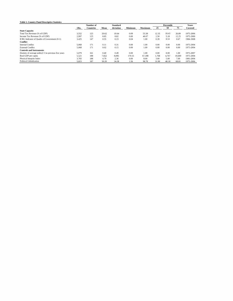
25 50 75
State Capacity
Total Tax Revenue (% of GDP) 3,552 125 20.62 10.64 0.09 53.38 12.35 18.43 26.89 1975-2006
Income Tax Revenue (% of GDP) 2,997 125 8.85 8.82 0.00 40.07 2.50 5.18 12.25 1975-2000
ICRG Indicator of Quality of Government (0-1) 3,425 147 0.55 0.23 0.04 1.00 0.39 0.53 0.67 1984-2008
Conflict
Internal Conflict 5,068 171 0.11 0.31 0.00 1.00 0.00 0.00 0.00 1975-2004
External Conflict 5,068 171 0.02 0.15 0.00 1.00 0.00 0.00 0.00 1975-2004
Controls and Instruments
Dummy of average polity2>3 in previous five years 5,079 161 0.40 0.49 0.00 1.00 0.00 0.00 1.00 1975-2007
Real GDP per capita 5,521 188 7,822 8,085 170.55 67,188 1,768 4,767 10,600 1975-2004
Physical Integrity Index 3,783 188 4.79 2.36 0.00 8.00 3.00 5.00 7.00 1981-2004
Political Globalization 5,823 187 50.20 24.28 1.56 98.78 31.90 48.18 68.81 1975-2006
Table 1. Country Panel Descriptive Statistics
Obs.
Number of
Countries Mean
Standard
deviation Minimum Maximum
Percentile Years
Covered
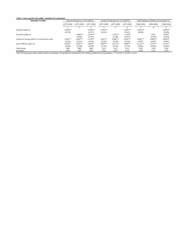
Dependent Variable
(1975-2004) (1975-2004) (1975-2004) (1975-2000) (1975-2000) (1975-2000) (1984-2004) (1984-2004) (1984-2004)
1 2 3 4 5 6 7 8 9
Internal Conflict (t) -5.049*** -4.939*** -2.570*** -2.505*** -0.091*** -0.093***
(0.378) (0.377) (0.319) (0.321) (0.009) (0.009)
External Conflict (t) -3.068*** -2.034*** -1.763*** -1.254** 0.021 0.038**
(0.844) (0.747) (0.649) (0.613) (0.016) (0.016)
Dummy of average polity2>3 in previous five years 5.100*** 5.065*** 5.116*** 4.581*** 4.566*** 4.592*** 0.096*** 0.090*** 0.096***
(0.425) (0.431) (0.425) (0.324) (0.326) (0.324) (0.007) (0.007) (0.007)
log of GDP per capita (t) 4.284*** 4.492*** 4.283*** 4.090*** 4.193*** 4.089*** 0.115*** 0.121*** 0.115***
(0.189) (0.188) (0.188) (0.143) (0.143) (0.142) (0.003) (0.003) (0.003)
Observations 2882 2882 2882 2515 2515 2515 2706 2706 2706
R-squared 0.426 0.407 0.427 0.515 0.507 0.515 0.569 0.551 0.570
Note: The regressions in these tables include year dummies. All equations are estimated by OLS. Robust standard errors in parentheses. *** p<0.01, ** p<0.05, * p<0.1.
Table 2- State capacitiy and conflict : Baseline OLS estimations
ICRG Indicator of Quality of Government (t) Total Tax Revenue as a % of GDP (t) Income Tax Revenue as a % of GDP (t)
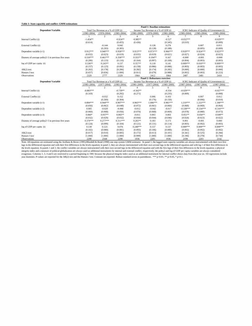
Dependent Variable
(1981-2004) (1976-2004) (1981-2004) (1981-2000) (1976-2000) (1981-2000) (1985-2004) (1985-2004) (1985-2004)
1 2 3 4 5 6 7 8 9
Internal Conflict (t) -1.454** -0.924** -0.985** -0.527 -0.032*** -0.029***
(0.614) (0.455) (0.436) (0.345) (0.010) (0.009)
External Conflict (t) -0.144 0.042 0.128 0.276 0.007 0.011
(0.293) (0.305) (0.128) (0.188) (0.005) (0.009)
Dependent variable (t-1) 0.912*** 0.940*** 0.958*** 0.913*** 0.973*** 0.966*** 0.918*** 0.924*** 0.923***
(0.032) (0.023) (0.019) (0.035) (0.019) (0.021) (0.027) (0.024) (0.023)
Dummy of average polity2>3 in previous five years 0.550*** 0.461*** 0.358*** 0.355** 0.194** 0.167 -0.000 -0.001 -0.000
(0.206) (0.133) (0.116) (0.164) (0.097) (0.108) (0.004) (0.003) (0.003)
log of GDP per capita (t) 0.336** 0.243** 0.137 0.357** 0.118 0.141 0.009*** 0.010*** 0.009***
(0.157) (0.123) (0.091) (0.158) (0.086) (0.088) (0.003) (0.003) (0.003)
AR(2) test [0.202] [0.178] [0.206] [0.282] [0.174] [0.285] [0.000] [0.000] [0.000]
Hansen J test [0.657] [0.836] [1.000] [0.911] [0.679] [0.988] [0.002] [0.003] [0.223]
Observations 2329 2777 2329 1964 2412 1964 2487 2481 2410
Dependent Variable
(1981-2004) (1977-2004) (1981-2004) (1981-2000) (1977-2004) (1981-2000) (1987-2004) (1987-2004) (1987-2004)
1 2 3 4 5 6 7 8 9
Internal Conflict (t) -0.883*** -0.739** -0.562** -0.354 -0.029*** -0.027***
(0.319) (0.292) (0.271) (0.235) (0.009) (0.008)
External Conflict (t) -0.032 0.152 0.006 0.103 0.007 0.012
(0.269) (0.304) (0.176) (0.150) (0.006) (0.010)
Dependent variable (t-1) 0.894*** 0.944*** 0.907*** 0.965*** 1.006*** 0.981*** 1.210*** 1.222*** 1.190***
(0.056) (0.062) (0.048) (0.072) (0.061) (0.066) (0.068) (0.069) (0.064)
Dependent variable (t-2) 0.005 -0.029 -0.000 -0.012 -0.042 -0.017 -0.338*** -0.334*** -0.316***
(0.060) (0.068) (0.056) (0.070) (0.068) (0.069) (0.078) (0.080) (0.073)
Dependent variable (t-3) 0.060* 0.057** 0.065** -0.011 0.003 0.003 0.051** 0.050** 0.049**
(0.032) (0.029) (0.032) (0.044) (0.044) (0.046) (0.024) (0.023) (0.022)
Dummy of average polity2>3 in previous five years 0.370*** 0.277*** 0.311*** 0.265** 0.183 0.173 0.001 -0.001 0.000
(0.124) (0.099) (0.104) (0.121) (0.131) (0.114) (0.003) (0.002) (0.003)
log of GDP per capita (t) 0.130 0.123 0.076 0.240*** 0.157 0.137 0.009*** 0.009*** 0.009***
(0.102) (0.080) (0.081) (0.093) (0.106) (0.089) (0.002) (0.002) (0.002)
AR(2) test [0.017] [0.010] [0.005] [0.172] [0.013] [0.101] [0.341] [0.525] [0.284]
Hansen J test [1.000] [1.000] [1.000] [0.999] [1.000] [1.000] [0.196] [0.278] [0.730]
Observations 2298 2568 2298 1936 2205 1936 2199 2203 2142
Table 3- State capacitiy and conflict: GMM estimations
Panel 1: Baseline estimations
Note: All equations are estimated using the Arellano & Bover (1995)/Blundell & Bond (1998) one step system GMM estimator. In panel 1, the lagged state capacity variables are always instrumented with their own first
lags in the differenced equation and with their first differences in the levels equation; in panel 2, they are always instrumented with their own second lags in the differenced equation and with lag 1 of their first differences in
the levels equation. In panels 1 and 2, the conflict variables are always instrumented with their own second lags in the differenced equation and with the first lags of their first differences in the levels equation; a physical
integrity index and a measure of political globalization are always used as additional instruments for internal and external conflict, respectively; the polity2 and log of GDP per capita variables are always considered
exogenous. Columns 1, 3, 4 and 6 are restricted to a period beginning in 1981 because the physical integrity index used as an additional instrument for internal conflict shows data from that year on. All regressions include
year dummies. P-values are reported for the AR(2) test and the Hansen J test. Constant not reported. Robust standard errors in parentheses. *** p<0.01, ** p<0.05, * p<0.1.
Total Tax Revenue as a % of GDP (t) ICRG Indicator of Quality of Government (t)Income Tax Revenue as a % of GDP (t)
Panel 2: Robustness exercises
ICRG Indicator of Quality of Government (t)Income Tax Revenue as a % of GDP (t)Total Tax Revenue as a % of GDP (t)
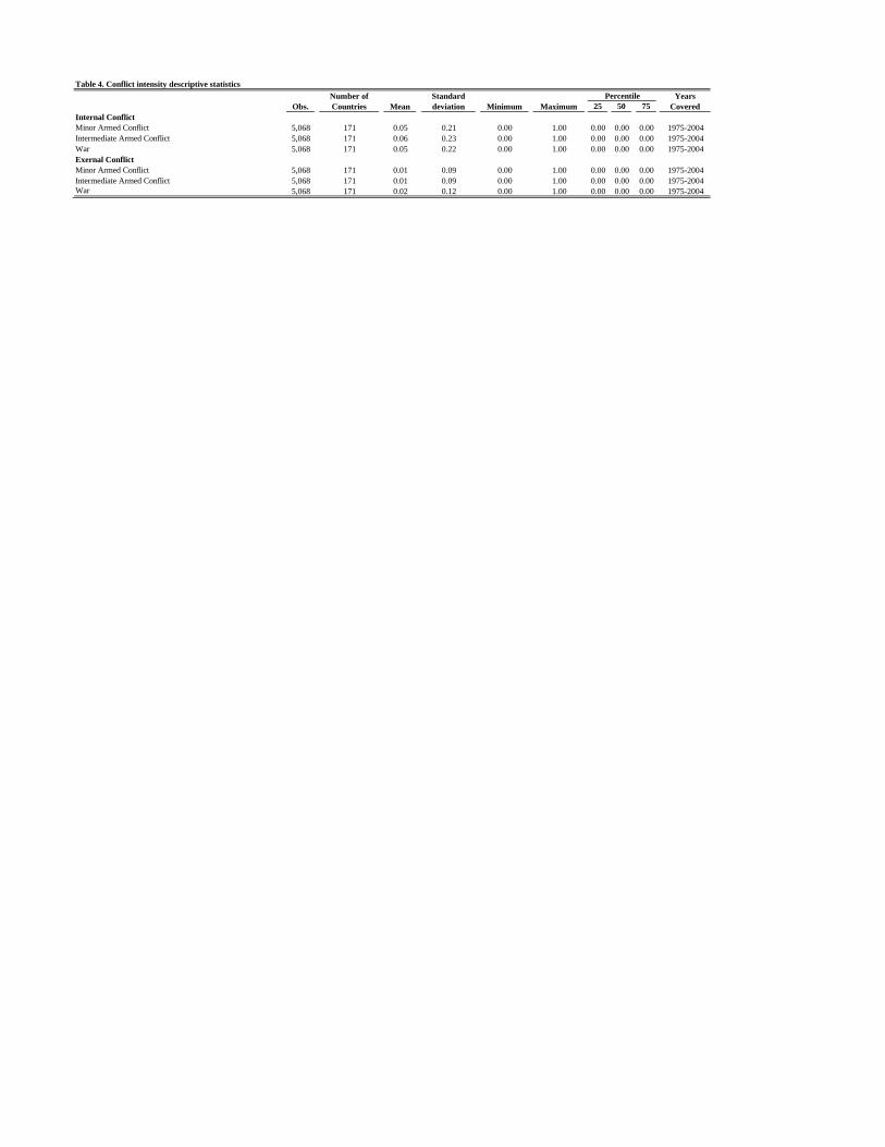
25 50 75
Internal Conflict
Minor Armed Conflict 5,068 171 0.05 0.21 0.00 1.00 0.00 0.00 0.00 1975-2004
Intermediate Armed Conflict 5,068 171 0.06 0.23 0.00 1.00 0.00 0.00 0.00 1975-2004
War 5,068 171 0.05 0.22 0.00 1.00 0.00 0.00 0.00 1975-2004
Exernal Conflict
Minor Armed Conflict 5,068 171 0.01 0.09 0.00 1.00 0.00 0.00 0.00 1975-2004
Intermediate Armed Conflict 5,068 171 0.01 0.09 0.00 1.00 0.00 0.00 0.00 1975-2004
War 5,068 171 0.02 0.12 0.00 1.00 0.00 0.00 0.00 1975-2004
Table 4. Conflict intensity descriptive statistics
Obs.
Number of
Countries Mean
Standard
deviation Minimum Maximum
Percentile Years
Covered
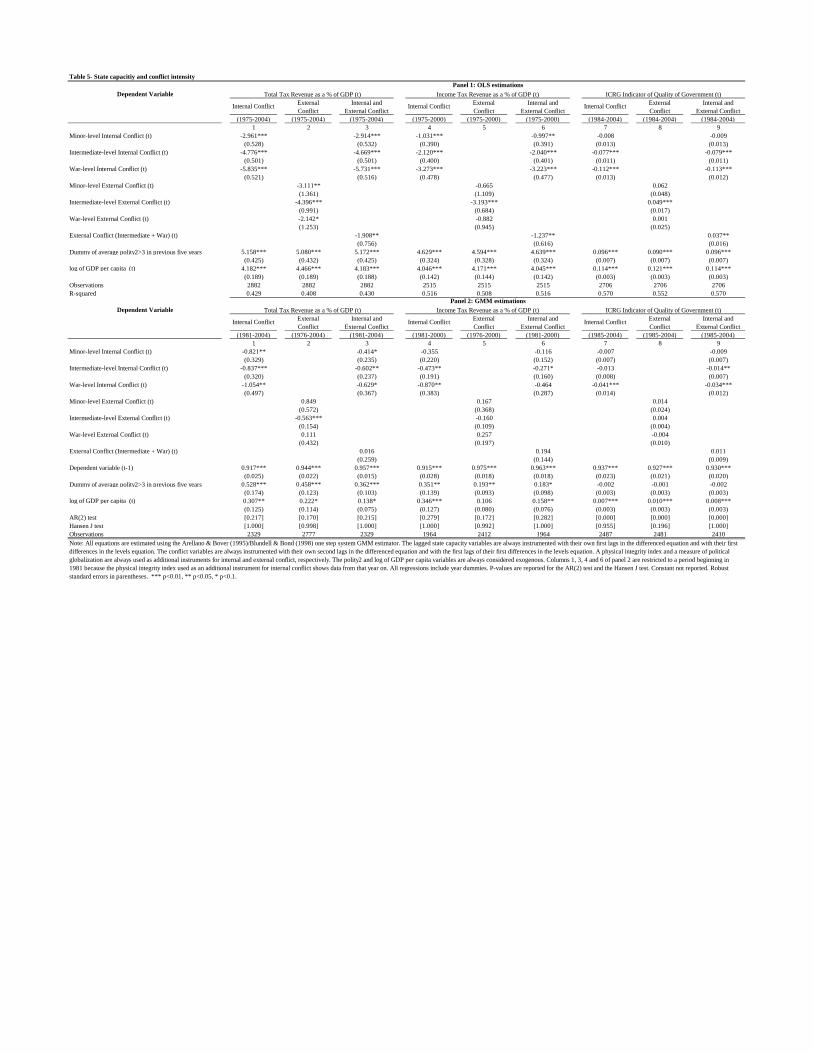
Dependent Variable
(1975-2004) (1975-2004) (1975-2004) (1975-2000) (1975-2000) (1975-2000) (1984-2004) (1984-2004) (1984-2004)
1 2 3 4 5 6 7 8 9
Minor-level Internal Conflict (t) -2.961*** -2.914*** -1.031*** -0.997** -0.008 -0.009
(0.528) (0.532) (0.390) (0.391) (0.013) (0.013)
Intermediate-level Internal Conflict (t) -4.776*** -4.669*** -2.120*** -2.040*** -0.077*** -0.079***
(0.501) (0.501) (0.400) (0.401) (0.011) (0.011)
War-level Internal Conflict (t) -5.835*** -5.731*** -3.273*** -3.223*** -0.112*** -0.113***
(0.521) (0.516) (0.478) (0.477) (0.013) (0.012)
Minor-level External Conflict (t) -3.111** -0.665 0.062
(1.361) (1.109) (0.048)
Intermediate-level External Conflict (t) -4.396*** -3.193*** 0.049***
(0.991) (0.684) (0.017)
War-level External Conflict (t) -2.142* -0.882 0.001
(1.253) (0.945) (0.025)
External Conflict (Intermediate + War) (t) -1.908** -1.237** 0.037**
(0.756) (0.616) (0.016)
Dummy of average polity2>3 in previous five years 5.158*** 5.080*** 5.172*** 4.629*** 4.594*** 4.639*** 0.096*** 0.090*** 0.096***
(0.425) (0.432) (0.425) (0.324) (0.328) (0.324) (0.007) (0.007) (0.007)
log of GDP per capita (t) 4.182*** 4.466*** 4.183*** 4.046*** 4.171*** 4.045*** 0.114*** 0.121*** 0.114***
(0.189) (0.189) (0.188) (0.142) (0.144) (0.142) (0.003) (0.003) (0.003)
Observations 2882 2882 2882 2515 2515 2515 2706 2706 2706
R-squared 0.429 0.408 0.430 0.516 0.508 0.516 0.570 0.552 0.570
Dependent Variable
(1981-2004) (1976-2004) (1981-2004) (1981-2000) (1976-2000) (1981-2000) (1985-2004) (1985-2004) (1985-2004)
1 2 3 4 5 6 7 8 9
Minor-level Internal Conflict (t) -0.821** -0.414* -0.355 -0.116 -0.007 -0.009
(0.329) (0.235) (0.220) (0.152) (0.007) (0.007)
Intermediate-level Internal Conflict (t) -0.837*** -0.602** -0.473** -0.271* -0.013 -0.014**
(0.320) (0.237) (0.191) (0.160) (0.008) (0.007)
War-level Internal Conflict (t) -1.054** -0.629* -0.870** -0.464 -0.041*** -0.034***
(0.497) (0.367) (0.383) (0.287) (0.014) (0.012)
Minor-level External Conflict (t) 0.849 0.167 0.014
(0.572) (0.368) (0.024)
Intermediate-level External Conflict (t) -0.563*** -0.160 0.004
(0.154) (0.109) (0.004)
War-level External Conflict (t) 0.111 0.257 -0.004
(0.432) (0.197) (0.010)
External Conflict (Intermediate + War) (t) 0.016 0.194 0.011
(0.259) (0.144) (0.009)
Dependent variable (t-1) 0.917*** 0.944*** 0.957*** 0.915*** 0.975*** 0.963*** 0.937*** 0.927*** 0.930***
(0.025) (0.022) (0.015) (0.028) (0.018) (0.018) (0.023) (0.021) (0.020)
Dummy of average polity2>3 in previous five years 0.528*** 0.458*** 0.362*** 0.351** 0.193** 0.183* -0.002 -0.001 -0.002
(0.174) (0.123) (0.103) (0.139) (0.093) (0.098) (0.003) (0.003) (0.003)
log of GDP per capita (t) 0.307** 0.222* 0.138* 0.346*** 0.106 0.158** 0.007*** 0.010*** 0.008***
(0.125) (0.114) (0.075) (0.127) (0.080) (0.076) (0.003) (0.003) (0.003)
AR(2) test [0.217] [0.170] [0.215] [0.279] [0.172] [0.282] [0.000] [0.000] [0.000]
Hansen J test [1.000] [0.998] [1.000] [1.000] [0.992] [1.000] [0.955] [0.196] [1.000]
Observations 2329 2777 2329 1964 2412 1964 2487 2481 2410
Table 5- State capacitiy and conflict intensity
Panel 1: OLS estimations
Total Tax Revenue as a % of GDP (t) Income Tax Revenue as a % of GDP (t) ICRG Indicator of Quality of Government (t)
Income Tax Revenue as a % of GDP (t) ICRG Indicator of Quality of Government (t)
Panel 2: GMM estimations
Internal and
External ConflictInternal Conflict
External
Conflict
Internal and
External ConflictInternal Conflict
External
Conflict
Internal and
External ConflictInternal Conflict
Internal and
External Conflict
Note: All equations are estimated using the Arellano & Bover (1995)/Blundell & Bond (1998) one step system GMM estimator. The lagged state capacity variables are always instrumented with their own first lags in the differenced equation and with their first
differences in the levels equation. The conflict variables are always instrumented with their own second lags in the differenced equation and with the first lags of their first differences in the levels equation. A physical integrity index and a measure of political
globalization are always used as additional instruments for internal and external conflict, respectively. The polity2 and log of GDP per capita variables are always considered exogenous. Columns 1, 3, 4 and 6 of panel 2 are restricted to a period beginning in
1981 because the physical integrity index used as an additional instrument for internal conflict shows data from that year on. All regressions include year dummies. P-values are reported for the AR(2) test and the Hansen J test. Constant not reported. Robust
standard errors in parentheses. *** p<0.01, ** p<0.05, * p<0.1.
Internal ConflictExternal
Conflict
Internal and
External ConflictInternal Conflict
External
Conflict
External
Conflict
Internal and
External ConflictInternal Conflict
External
Conflict
Total Tax Revenue as a % of GDP (t)
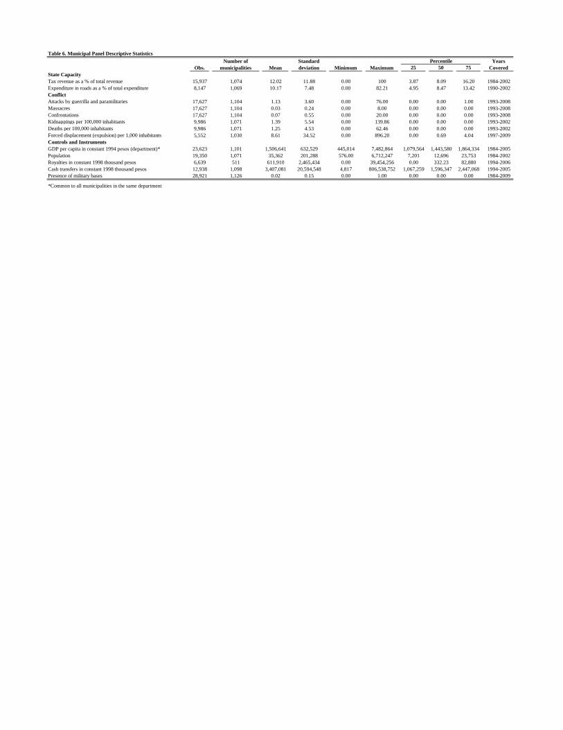
25 50 75
State Capacity
Tax revenue as a % of total revenue 15,937 1,074 12.02 11.88 0.00 100 3.87 8.09 16.20 1984-2002
Expenditure in roads as a % of total expenditure 8,147 1,069 10.17 7.48 0.00 82.21 4.95 8.47 13.42 1990-2002
Conflict
Attacks by guerrilla and paramilitaries 17,627 1,104 1.13 3.60 0.00 76.00 0.00 0.00 1.00 1993-2008
Massacres 17,627 1,104 0.03 0.24 0.00 8.00 0.00 0.00 0.00 1993-2008
Confrontations 17,627 1,104 0.07 0.55 0.00 20.00 0.00 0.00 0.00 1993-2008
Kidnappings per 100,000 inhabitants 9,986 1,071 1.39 5.54 0.00 139.86 0.00 0.00 0.00 1993-2002
Deaths per 100,000 inhabitants 9,986 1,071 1.25 4.53 0.00 62.46 0.00 0.00 0.00 1993-2002
Forced displacement (expulsion) per 1,000 inhabitants 5,552 1,030 8.61 34.52 0.00 896.20 0.00 0.69 4.04 1997-2009
Controls and Instruments
GDP per capita in constant 1994 pesos (department)* 23,623 1,101 1,506,641 632,529 445,014 7,482,864 1,079,564 1,443,580 1,864,334 1984-2005
Population 19,350 1,071 35,362 201,288 576.00 6,712,247 7,201 12,696 23,753 1984-2002
Royalties in constant 1998 thousand pesos 6,639 511 611,910 2,465,434 0.00 39,454,256 0.00 332.23 82,880 1994-2006
Cash transfers in constant 1998 thousand pesos 12,938 1,098 3,407,081 20,594,548 4,817 806,538,752 1,067,259 1,596,347 2,447,068 1994-2005
Presence of military bases 28,921 1,126 0.02 0.15 0.00 1.00 0.00 0.00 0.00 1984-2009
*Common to all municipalities in the same department
Years
Covered
Table 6. Municipal Panel Descriptive Statistics
Percentile
Obs.
Number of
municipalities Mean
Standard
deviation Minimum Maximum
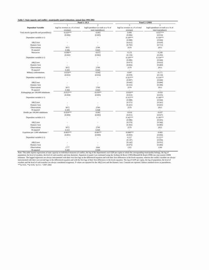
1 2 3 4
Dependent Variable log(Tax revenue as a % of total
revenue)
log(Expenditure in roads as a % of
total expenditure)
log(Tax revenue as a % of total
revenue)
log(Expenditure in roads as a % of
total expenditure)
Total attacks (guerrilla and paramilitary) -0.020*** -0.003 0.006 -0.037***
(0.006) (0.005) (0.006) (0.014)
Dependent variable (t-1) - - 0.329*** 0.150***
(0.088) (0.044)
AR(2) test - - [0.612] [0.620]
Hansen J test - - [0.792] [0.711]
Observations 3072 2709 2579 2013
R-squared 0.306 0.045 - -
Massacres -0.090** -0.075 -0.131 -0.249
(0.042) (0.062) (0.116) (0.202)
Dependent variable (t-1) - - 0.329*** 0.154***
(0.086) (0.044)
AR(2) test - - [0.675] [0.622]
Hansen J test - - [0.856] [0.460]
Observations 3072 2709 2579 2013
R-squared 0.303 0.045 - -
Military confrontations -0.054** -0.042 -0.007 -0.171
(0.022) (0.032) (0.019) (0.114)
Dependent variable (t-1) - - 0.323*** 0.154***
(0.087) (0.044)
AR(2) test - - [0.642] [0.684]
Hansen J test - - [0.555] [0.596]
Observations 3072 2709 2579 2013
R-squared 0.304 0.043 - -
Kidnappings per 100,000 inhabitants -0.012*** -0.010** -0.026** -0.018
(0.004) (0.005) (0.013) (0.015)
Dependent variable (t-1) - - 0.315*** 0.148***
(0.088) (0.044)
AR(2) test - - [0.571] [0.561]
Hansen J test - - [0.421] [0.641]
Observations 3072 2709 2579 2013
R-squared 0.305 0.048 - -
Deaths per 100,000 inhabitants -0.024*** -0.001 -0.016 -0.037
(0.004) (0.003) (0.011) (0.027)
Dependent variable (t-1) - - 0.342*** 0.146***
(0.086) (0.045)
AR(2) test - - [0.570] [0.566]
Hansen J test - - [0.365] [0.085]
Observations 3072 2709 2579 2013
R-squared 0.312 0.045 - -
Expulsion per 1,000 inhabitants ⅟ -0.003*** -0.001** -0.008*** -0.003
(0.001) (0.000) (0.003) (0.004)
Dependent variable (t-1) - - 0.227 0.122**
(0.147) (0.056)
AR(2) test - - [0.142] [0.951]
Hansen J test - - [0.675] [0.466]
Observations 1777 1644 1355 1190
R-squared 0.341 0.044 - -
Note: This table reports regressions of state capacity on individual measures of conflict, the log of the department's real GDP per capita to which the corresponding municipality belongs, the log of
population, the level of royalties, the level of cash transfers and time dummies. Equations in panel 2 are estimated using the Arellano & Bover (1995)/Blundell & Bond (1998) one step system GMM
estimator. The lagged regressors are always instrumented with their own first lags in the differenced equation and with their first differences in the levels equation, whereas the conflict variables are always
instrumented with their own second lags in the differenced equation and with the first lags of their first differences in the levels equation. The log of GDP per capita, the log of population, the level of
royalties and the level of cash transfers are always considered exogenous. P-values are reported for the AR(2) test and the Hansen J test. Constant not reported. Robust standard errors in parentheses.
***p<0.01, **p<0.05, *p<0.1. ⅟1997-2002
Table 7- State capacity and conflict : municipality panel estimations, annual data 1994-2002
Panel 1: OLS Panel 2: GMM
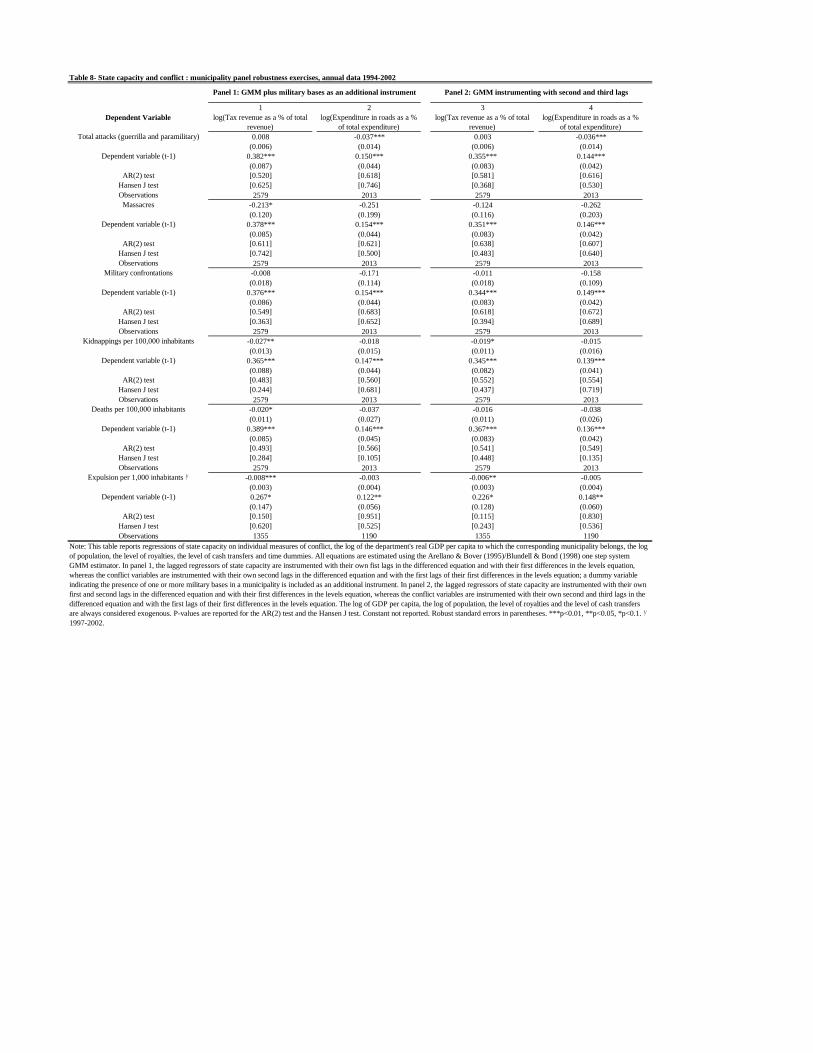
1 2 3 4
Dependent Variable log(Tax revenue as a % of total
revenue)
log(Expenditure in roads as a %
of total expenditure)
log(Tax revenue as a % of total
revenue)
log(Expenditure in roads as a %
of total expenditure)
Total attacks (guerrilla and paramilitary) 0.008 -0.037*** 0.003 -0.036***
(0.006) (0.014) (0.006) (0.014)
Dependent variable (t-1) 0.382*** 0.150*** 0.355*** 0.144***
(0.087) (0.044) (0.083) (0.042)
AR(2) test [0.520] [0.618] [0.581] [0.616]
Hansen J test [0.625] [0.746] [0.368] [0.530]
Observations 2579 2013 2579 2013
Massacres -0.213* -0.251 -0.124 -0.262
(0.120) (0.199) (0.116) (0.203)
Dependent variable (t-1) 0.378*** 0.154*** 0.351*** 0.146***
(0.085) (0.044) (0.083) (0.042)
AR(2) test [0.611] [0.621] [0.638] [0.607]
Hansen J test [0.742] [0.500] [0.483] [0.640]
Observations 2579 2013 2579 2013
Military confrontations -0.008 -0.171 -0.011 -0.158
(0.018) (0.114) (0.018) (0.109)
Dependent variable (t-1) 0.376*** 0.154*** 0.344*** 0.149***
(0.086) (0.044) (0.083) (0.042)
AR(2) test [0.549] [0.683] [0.618] [0.672]
Hansen J test [0.363] [0.652] [0.394] [0.689]
Observations 2579 2013 2579 2013
Kidnappings per 100,000 inhabitants -0.027** -0.018 -0.019* -0.015
(0.013) (0.015) (0.011) (0.016)
Dependent variable (t-1) 0.365*** 0.147*** 0.345*** 0.139***
(0.088) (0.044) (0.082) (0.041)
AR(2) test [0.483] [0.560] [0.552] [0.554]
Hansen J test [0.244] [0.681] [0.437] [0.719]
Observations 2579 2013 2579 2013
Deaths per 100,000 inhabitants -0.020* -0.037 -0.016 -0.038
(0.011) (0.027) (0.011) (0.026)
Dependent variable (t-1) 0.389*** 0.146*** 0.367*** 0.136***
(0.085) (0.045) (0.083) (0.042)
AR(2) test [0.493] [0.566] [0.541] [0.549]
Hansen J test [0.284] [0.105] [0.448] [0.135]
Observations 2579 2013 2579 2013
Expulsion per 1,000 inhabitants ⅟ -0.008*** -0.003 -0.006** -0.005
(0.003) (0.004) (0.003) (0.004)
Dependent variable (t-1) 0.267* 0.122** 0.226* 0.148**
(0.147) (0.056) (0.128) (0.060)
AR(2) test [0.150] [0.951] [0.115] [0.830]
Hansen J test [0.620] [0.525] [0.243] [0.536]
Observations 1355 1190 1355 1190
Table 8- State capacity and conflict : municipality panel robustness exercises, annual data 1994-2002
Panel 1: GMM plus military bases as an additional instrument Panel 2: GMM instrumenting with second and third lags
Note: This table reports regressions of state capacity on individual measures of conflict, the log of the department's real GDP per capita to which the corresponding municipality belongs, the log
of population, the level of royalties, the level of cash transfers and time dummies. All equations are estimated using the Arellano & Bover (1995)/Blundell & Bond (1998) one step system
GMM estimator. In panel 1, the lagged regressors of state capacity are instrumented with their own fist lags in the differenced equation and with their first differences in the levels equation,
whereas the conflict variables are instrumented with their own second lags in the differenced equation and with the first lags of their first differences in the levels equation; a dummy variable
indicating the presence of one or more military bases in a municipality is included as an additional instrument. In panel 2, the lagged regressors of state capacity are instrumented with their own
first and second lags in the differenced equation and with their first differences in the levels equation, whereas the conflict variables are instrumented with their own second and third lags in the
differenced equation and with the first lags of their first differences in the levels equation. The log of GDP per capita, the log of population, the level of royalties and the level of cash transfers
are always considered exogenous. P-values are reported for the AR(2) test and the Hansen J test. Constant not reported. Robust standard errors in parentheses. ***p<0.01, **p<0.05, *p<0.1. ⅟
1997-2002.