Embed Size (px)
Citation preview
Abby Almonte, Crystal Chea, Anthony Yoohanna 2/6/2012
Extra Credit Assignment
Solution & Report

2
Table of Contents
Problem Statement ...................................................................................................................................................................................... 3
Original Problem Statement Assumptions .................................................................................................................................................. 4
Manual Formulation of Problem ................................................................................................................................................................. 5
Part A ....................................................................................................................................................................................................... 6
Part B ....................................................................................................................................................................................................... 8
Part C ....................................................................................................................................................................................................... 9
Original Problem Statement: WinQSB Solution ...................................................................................................................................... 10
Data input for WinQSB “Queuing Analysis” ........................................................................................................................................ 10
Cost Assumptions .................................................................................................................................................................................. 11
Part A: WinQSB .................................................................................................................................................................................... 13
Part B: WinQSB .................................................................................................................................................................................... 14
Part C: WinQSB .................................................................................................................................................................................... 15
WinQSB Summary Analysis .................................................................................................................................................................... 16
Sensitivity Analysis: ................................................................................................................................................................................. 17
Number of Servers: ................................................................................................................................................................................ 17
Service Rate: .......................................................................................................................................................................................... 23
Arrival Rate: .......................................................................................................................................................................................... 26
Comparison between Manual Solution versus WinQSB .......................................................................................................................... 29
Report to Manager .................................................................................................................................................................................... 30

3
Problem Statement
An average of 40 cars per hour, which are exponentially distributed, are tempted to use the drive-in at the Hot Dog King Restaurant.
If more than 4 cars are in the line, including the car at the window, a car will not enter the line. It takes an average of 4 minutes to
serve a car.
a) What is the average number of cars waiting for the drive-in window? (not including the car at the window)
b) On the average, how many cars will be served per hour?
c) If a customer just joined the line to the drive-in window, on average how long will it be until he or she has received their food?
4
Original Problem Statement Assumptions
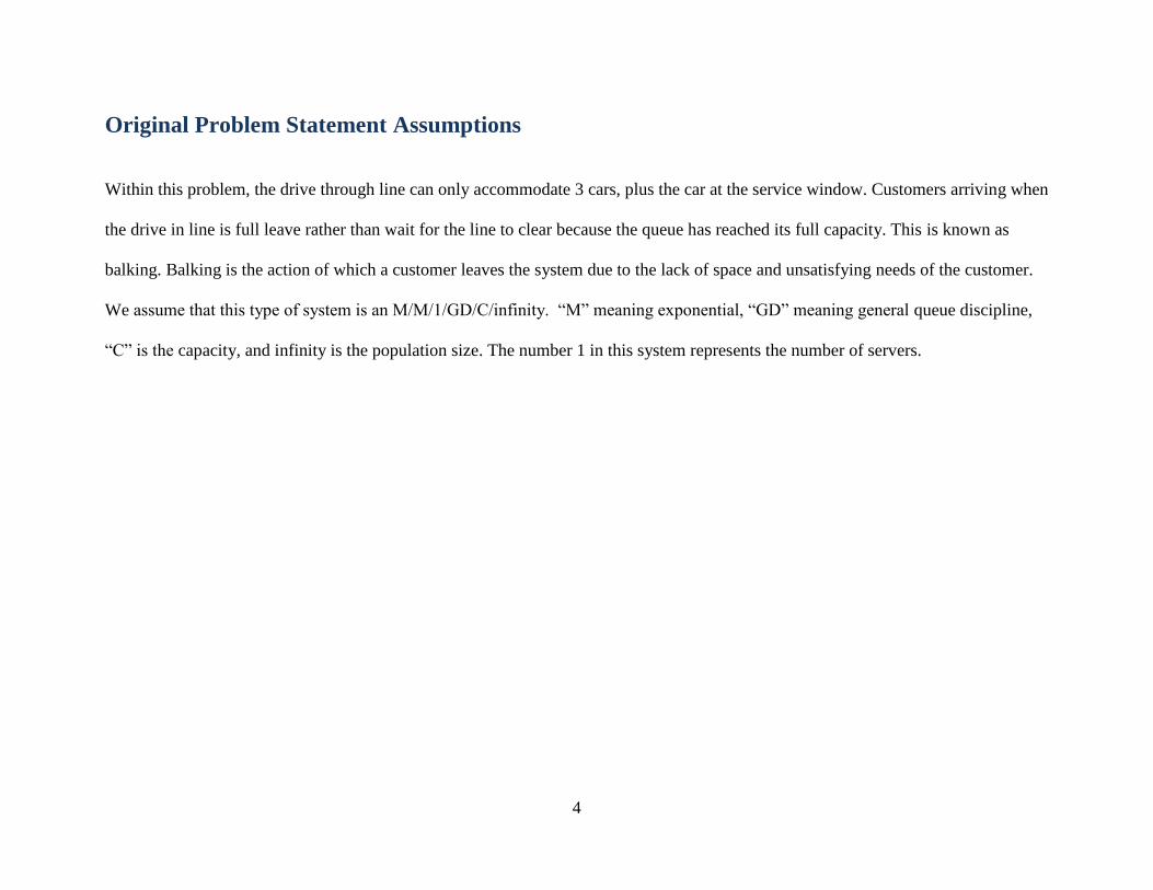
Within this problem, the drive through line can only accommodate 3 cars, plus the car at the service window. Customers arriving when
the drive in line is full leave rather than wait for the line to clear because the queue has reached its full capacity. This is known as
balking. Balking is the action of which a customer leaves the system due to the lack of space and unsatisfying needs of the customer.
We assume that this type of system is an M/M/1/GD/C/infinity. “M” meaning exponential, “GD” meaning general queue discipline,
“C” is the capacity, and infinity is the population size. The number 1 in this system represents the number of servers.

5
Manual Formulation of Problem
To begin, we identify what the arrival rate, is which is given in the problem statement:
Arrival Rate (λ) = 40 cars per hour
Then to find the service rate, we use the average service time per customer which is 4 minutes, and we calculate how many customers
can be served within an hour time.
Service Rate (μ) = 15 cars per hour
Next, we must find the traffic intensity - rho (ρ)
Traffic Intensity is a measure of how occupied a server is which vital in determining the amount of people or equipment needed to
develop a steady system.
Note that if rho (ρ) is greater than 1 then the system will blow up.
To find rho (ρ) we follow these calculations:
From these values we can now solve parts a, b, and c.
6
Part A
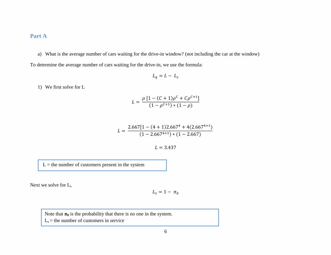
a) What is the average number of cars waiting for the drive-in window? (not including the car at the window)
To determine the average number of cars waiting for the drive-in, we use the formula:
1) We first solve for L
( )
( ) ( )
( ) ( )
( ) ( )
Next we solve for Ls
Note that π0 is the probability that there is no one in the system.
Ls = the number of customers in service
L = the number of customers present in the system

7
To find π0 we use the following equation
( )
( )
( )
( )
2) Now we solve for Lq
The average number of cars waiting for the drive – in window is about 3 cars.
*Refer to page 5 for variables that are not defined.
8
Part B
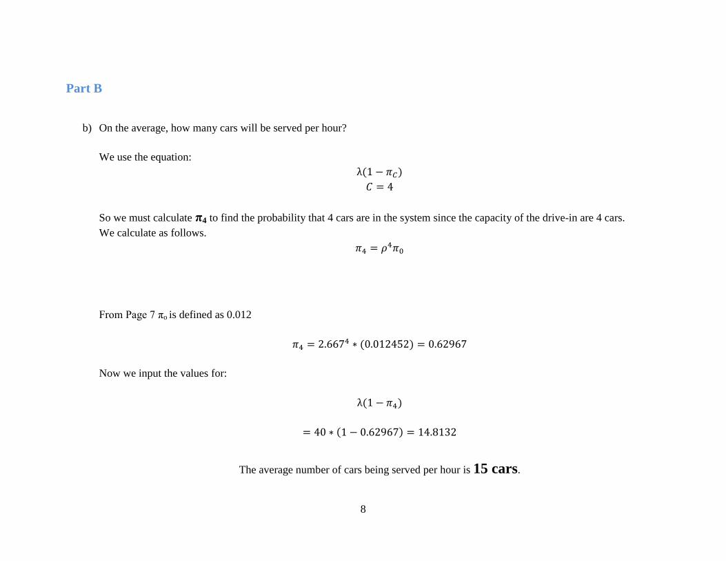
b) On the average, how many cars will be served per hour?
We use the equation:
( )
So we must calculate π4 to find the probability that 4 cars are in the system since the capacity of the drive-in are 4 cars.
We calculate as follows.
From Page 7 πo is defined as 0.012
( )
Now we input the values for:
( )
( )
The average number of cars being served per hour is 15 cars.
9
Part C
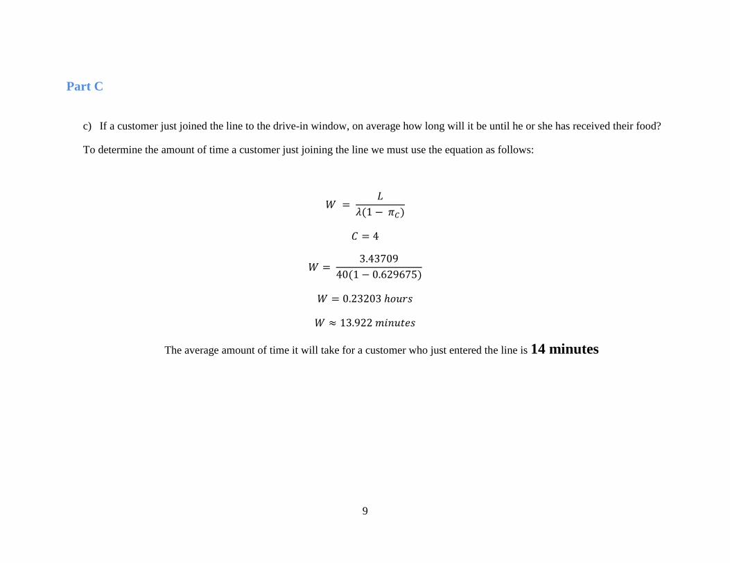
c) If a customer just joined the line to the drive-in window, on average how long will it be until he or she has received their food?
To determine the amount of time a customer just joining the line we must use the equation as follows:
( )
( )
The average amount of time it will take for a customer who just entered the line is 14 minutes

10
Original Problem Statement: WinQSB Solution
Data input for WinQSB “Queuing Analysis”
Figure 1.1
When working with WinQSB, our team input all of the data from the question, which covered the number of servers, service
rate per hour, customer arrival rate per hour, queue capacity, and the customer population. The values that require cost were fabricated
by our team since all cost values are subjective.

11
Cost Assumptions
We assume the cost of busy server cost per hour was marked at $10 because we believe that a worker at a fast food restaurant
with a drive-in usually earned $10 an hour on the high end. The idle server cost per hour represents how much a server would get paid
when they are idle, and we placed that value at $8 because that is minimum wage. Therefore, even a worker is not busy; they still
need to get paid the base wage. The customer waiting cost per hour represents how much money the business loses when a customer
waits for an hour. We assume that if a customer has to wait that long, their food should be free to compensate for the delay. We also
assume that the average cost for food through a drive in cost $10. The cost of customers being served per hour represents how much
money the company spends when we serve customers in an hour. We included costs of labor, machine costs, and the utility costs. The
cost of a customer being balked was set at $18 since balking is when the customer does not enter the system; we used the average cost
of a meal and the cost of losing a customer which sums up to $20, so we chose a number in between $10 - $20. The unit queue
capacity cost represents how much money it cost per space in a queue, and this was placed at $10 because this is the amount the
restaurant has to pay for rent for taking up space.

12
Figure 1.2
Figure 1.2 shows a table of the performance measures and the results from entering in the information from Figure 1.1 into WinQSB. It shows
information such as the system utilization, the average number of customers in the queue, the average time a customer spends in a queue, and a
probability of a system being busy. This table also shows how much the company would be paying for each factor, and the total price of the whole
system. Line number 20 shows that the total cost of customers being balked per hour is $453.36, which is the majority of the hourly cost of the system.

13
Part A: WinQSB
a) What is the average number of cars waiting for the drive-in window? (not including the car at the window)
Figure 1.3
Average number of cars (customers) waiting in the drive-in = 2.4498
About 3 Cars waiting in the drive-in window
*In Figure 1.3, the red box highlights the avergae number of customers in the queue.

14
Part B: WinQSB
On the average, how many cars will be served per hour?
Figure 1.4
Average amount of cars served per hour = 14.8132
About 15 Cars served per hour
*In Figure 1.4, the red box highlights the avergae amount of cars being served per hour.

15
Part C: WinQSB
b) If a customer just joined the line to the drive-in window, on average how long will it be until he or she has received their food?
Figure 1.5
Time it takes for a customer to receive their food = 0.2320 hours
converted to minutes = 13.9 minutes
About 14 minutes until food is received
*In Figure 1.5, the red box highlights the avergae time a customer will receive their food.

16
WinQSB Summary Analysis
The WinQSB solutions were very close to our manually calculated solutions. The various server and customer costs we chose
for the WinQSB input had no effect on the solution to the problem other than showing hourly costs for the system. To go further, we
created extra questions that relate to the problem at hand.
1. What happens if the number of servers changes?
2. What happens if the average service time changes?
3. What happens if the arrival rate changes?
4. What can be done to reduce the hourly cost?
5. What is the best option for reducing the hourly cost?
Our team decided to perform sensitivity analysis on the arrival rate, service time, and number of servers and see what effect changes in
those variables on the solution and its related costs. With the sensitivity analysis we would be able to answer the questions and make
recommendations to the management that would help reduce the total hourly cost.

17
Sensitivity Analysis:
Number of Servers:
For our first sensitivity analysis, we chose to look at the number of servers. In the original problem statement, we currently only have
one server, but we wanted to see how the system would run differently if we had up to 5 servers.
Figure 1.6
Figure 1.6 shows the values that we chose for the sensitivity analysis for number of servers. We ran the program so that we would be able
to see the difference from 1 to 5 workers, in increments of 1.

18
Figure 1.7
Figure 1.7 shows the results of having 1 to 5 numbers of servers. Waiting time in line, or Wq, has decreased from 0.165 of an hour to
0.003 hours. By decreasing the waiting time in line, more customers would be served because a decreased time in line is proportional
to the number of customers in line. Although the waiting time in line and number of customers in line have all improved with more
servers, not all aspects of the business have improved. Certain costs have gone up because of labor wages such as the busy server cost
and the idle server cost. The busy server cost has increased from $9.87 to a max of $26.36 and the idle server cost went from $0.09 to
$18.91. The reason the prices are higher is because we have to pay the extra servers for working. The idle cost increased because since
there are more servers, each server has less work to complete on their own. Other costs decreased such as waiting customer costs,
because customers were not waiting in line as long and balked customer costs, because customers were not being balked with more
servers working. Overall, the total cost of the system continues to decrease with more workers.

19
Figure 1.8
Figure 1.8 is a graph that visually shows how the total cost of the system continues to decrease as the number of servers increase.
From 1 to 2 servers, there is a steep line, representing a large decrease in the total cost of the system per hour. From 4 to 5 servers, line
is more horizonal. This shows us that as the number of servers increase, the amount of money saved in the total cost of the system
$529.69
$314.70
$184.02
$130.24 $116.44
$-
$100.00
$200.00
$300.00
$400.00
$500.00
$600.00
1 2 3 4 5
Co
st
Number of Servers
Number of Servers Vs. Total Cost

20
decreases more with each server added. Our team decided to extend our sensitivity analysis to see what would happen with the total
cost of the system if more servers were added.
Figure 1.9
Figire 1.9 shows the results of having up to 7 servers in total. Even though the balk rate continues to decrease, the total cost of the
system starts to increase again because the idle server costs increases, due to a low system utilization.

21
Figure 1.10
Figure 1.10 visually shows us that although the increasing number of servers decreases the total cost of the system, if too many servers
are added, the cost of the system starts to increase again. Going back to question 1, what happens if the number of servers changes?
The answer is that the total cost of the system decreases until too many servers are added, and at that point, the total cost of the system
begins to rise again. The number of servers also has an effect on the effective arrival rate, system utilization, number of customers in
line, waiting time in line, and the number of customers bulked. The effective arrival rate increases, since more customers are being
$529.69
$314.70
$184.02
$130.24 $116.44 $117.78
$123.94
$-
$100.00
$200.00
$300.00
$400.00
$500.00
$600.00
1 2 3 4 5 6 7
Co
st
Number of Servers
Number of Servers Vs. Total Cost

22
served and the utilization decreases because more servers are working in parallel. The utilization is directly proportional to the number
of customers in line, and the waiting time in line. As the utilization decreases, so does the customers in line and the waiting time.

23
Service Rate:
For our second sensitivity analysis, we chose to look at the service rate. In the original problem statement, we currently only had a
service rate of 15 customers per hour, but we wanted to see how the system would run differently if we had a rate up to 25 customers
an hour. We only changed the service rate, and left all of the other factors in place of the original problem statement.
Figure 1.11

24
Figure 1.11 shows the set up for the service rate. We wanted to see how the service rate would change all of the other factors of this
problem. We started it from 12 customers an hour because we wanted to see how the system would run if a Hot Dog King server was
having a slow day, and up to 25 customers an hour to see how it would be if the service rate was faster. We did the increments in steps
of 1.
Figure 1.12

25
Figure 1.12 shows the results for changing the service rate in the problem. The waiting time in line, or Wq, decreases from 0.217 of an
hour to 0.082, which shows that customers are waiting for a shorter time. The busy server costs only decreases by 60 cents because
there is only one server working. The customer waiting cost decreases from $25.89 to $19.23 because customers are waiting in line for
less time. The balked customer cost decreases from $505 to $298, which shows that Hot Dog King is losing less customers from
customers being balked. Overall, the total cost of the system continues to decrease as the service rate increases because less money is
being lost from customers being balked. So going back to answer question 2, what happens if the average service time changes? If the
average service time changes, the waiting time in line, waiting customer cost, and balked customer cost all decrease, which causes the
total cost of the system to decrease. Even though the total cost decreases, it only decreased by about $200 with a 60% increase in
service time. Realistically, this is not possible because one server can only work so fast. Also the rate at which the food cooks cannot
be altered.
26
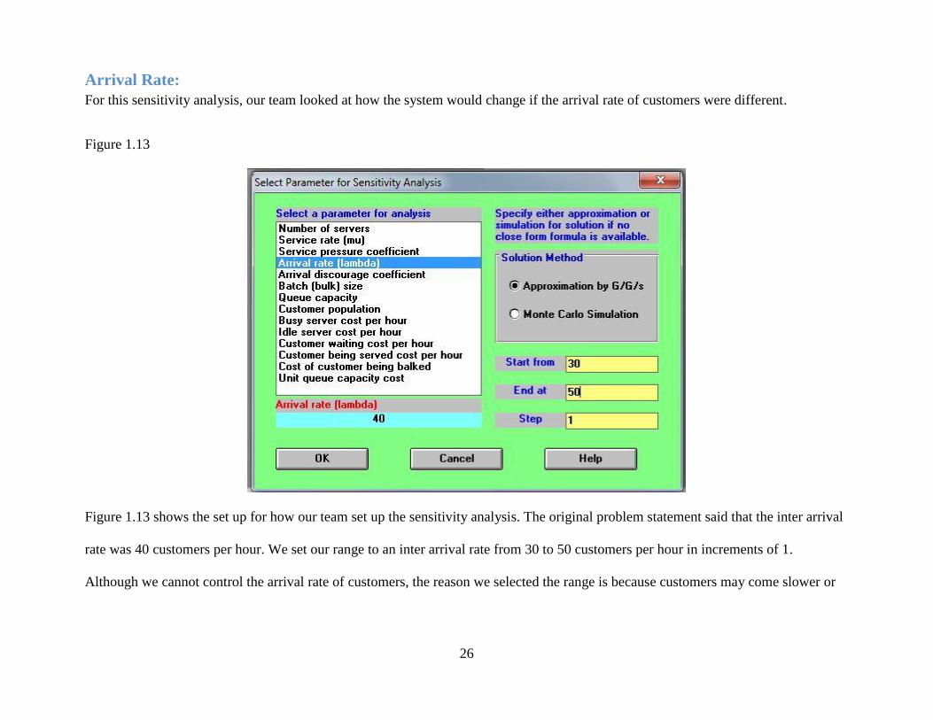
Arrival Rate:
For this sensitivity analysis, our team looked at how the system would change if the arrival rate of customers were different.
Figure 1.13
Figure 1.13 shows the set up for how our team set up the sensitivity analysis. The original problem statement said that the inter arrival
rate was 40 customers per hour. We set our range to an inter arrival rate from 30 to 50 customers per hour in increments of 1.
Although we cannot control the arrival rate of customers, the reason we selected the range is because customers may come slower or
27
faster depending on the day. If it is a holiday for example, customers will arrive at a slower rate, and if it is a Saturday, customers may
arrive at a faster rate.
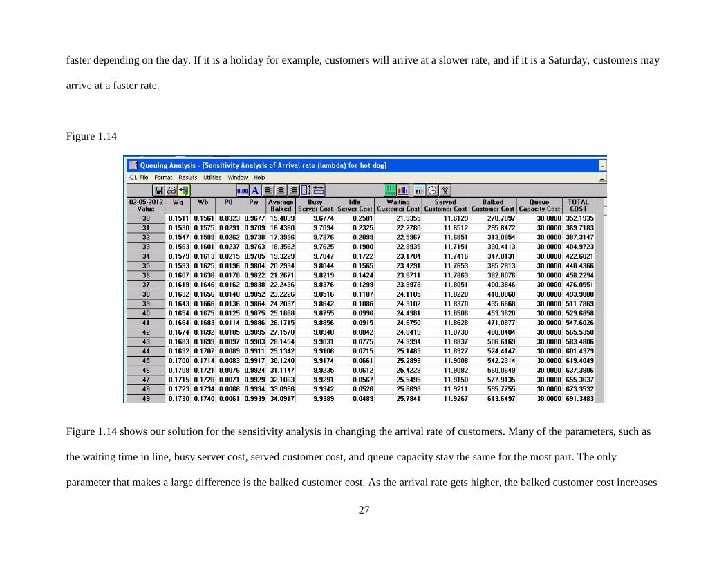
Figure 1.14
Figure 1.14 shows our solution for the sensitivity analysis in changing the arrival rate of customers. Many of the parameters, such as
the waiting time in line, busy server cost, served customer cost, and queue capacity stay the same for the most part. The only
parameter that makes a large difference is the balked customer cost. As the arrival rate gets higher, the balked customer cost increases

28
as well because more customers are leaving due to the system being full. To answer question number 3, what happens if the arrival
rate changes? If the arrival rate changes, average amount of customers are balked, causing the price of balked customer cost to
increase, which in turn affects the total cost. As the arrival rate increases, the total cost of the system increases as well.
Question number 4 asks, what can be done to reduce the hourly cost? The only parameter that we have control over is the amount of
servers. By increasing the servers to 5, the total cost of the system decreases to $116. A quicker service rate can also improve the total
cost of the system, but the service rate has to be reasonable. A lower arrival rate also reduces the hourly costs, but we have no control
on the arrival rate of customers.
Question number 5 asks, what is the best option for reducing the hourly cost? The best option for reducing the hourly cost is to have 5
servers working. The total cost of the system can drop down to $116 by just changing one parameter. Although labor costs will
increase, money will be saved in the balked customer cost.

29
Comparison between Manual Solution versus WinQSB Figure 1.15
Question Manual WinQSB
a)
What is the
average number
of cars waiting
for the drive-in
window?
3 cars 3 cars
b)
On the average,
how many cars
will be served
per hour?
15 cars 15 cars
c)
If a customer
just joined the
line to the drive-
in window, on
average how long
will it be until he
or she has
received their
food?
14 minutes 14 minutes
In Figure 1.15 is a chart that compares the results from manually solving the problem statement to using WinQSB. Using WinQSB is
a great way to double check your own work; however it is also very important to input the correct values and abbreviations. For
instance, if you were to change customer population to a number 4 instead of an “M” the results would have skewed from the real
values.

30
Report to Manager
Dear Manager,
The Hot Dog King drive through costs $529.69 per hour of operation. The biggest contributor to the hourly cost is the cost of
customers leaving when the drive through line is full. $453.36 per hour is lost due to customers refusing to wait for the line to clear.
The one server is almost never idle which indicates that the system is inadequate to handle the current volume of drive through
customers. Further analysis showed that increasing the service rate would be the only way to reduce hourly cost. Sensitivity analysis
was performed on the average service time as well as the number of servers. Even with a 40% reduction in average service time, the
hourly cost was only reduced to $368.82. Increasing the number of servers had a much greater effect as shown in the table below:
Servers Total Cost per Hour
1 $ 529.69
2 $ 314.70
3 $ 184.02
4 $ 130.24
5 $ 116.44
Adding one more server reduces total hourly cost more than decreasing average service time by 40%. In order to reduce the hourly
cost as much as possible, it is recommended that the company increase the number of servers from one to five. With five servers the
total hourly cost will drop to $116.44 with only $8.35 cost per hour due to lost customers.