Embed Size (px)
Citation preview
Vol.:(0123456789)
Optimization and Engineeringhttps://doi.org/10.1007/s11081-021-09643-x
1 3
RESEARCH ARTICLE
Extracting a low‑dimensional predictable time series
Yining Dong1 · S. Joe Qin2 · Stephen P. Boyd3
Received: 15 October 2020 / Revised: 16 March 2021 / Accepted: 10 May 2021 © The Author(s), under exclusive licence to Springer Science+Business Media, LLC, part of Springer Nature 2021
AbstractLarge scale multi-dimensional time series can be found in many disciplines, includ-ing finance, econometrics, biomedical engineering, and industrial engineering systems. It has long been recognized that the time dependent components of the vector time series often reside in a subspace, leaving its complement independent over time. In this paper we develop a method for projecting the time series onto a low-dimensional time-series that is predictable, in the sense that an auto-regressive model achieves low prediction error. Our formulation and method follow ideas from principal component analysis, so we refer to the extracted low-dimensional time series as principal time series. In one special case we can compute the optimal pro-jection exactly; in others, we give a heuristic method that seems to work well in practice. The effectiveness of the method is demonstrated on synthesized and real time series.
Keywords Time series · Dimension reduction · Feature extraction
* Yining Dong [email protected]
S. Joe Qin [email protected]
Stephen P. Boyd [email protected]
1 School of Data Science, City University of Hong Kong, Hong Kong, China2 School of Data Science and Hong Kong Institute for Data Science, Centre for Systems
Informatics Engineering, City University of Hong Kong, 83 Tat Chee Ave., Hong Kong, China3 Department of Electrical Engineering, Stanford University, Stanford, USA
Y. Dong et al.
1 3
1 Introduction
High dimensional time series analysis and applications have become increasingly important in many different domains. In many cases, the high dimensional time series data are both cross-correlated and auto-correlated. Cross-correlations among different time series make it possible to use a set of lower dimensional time series to represent the original, high dimensional time series. For example, principal compo-nent analysis (PCA) (Connor and Korajczyk 1986; Bai and Ng 2008) and general-ized PCA (Choi 2012) methods utilize the cross-correlations among different time series to extract lower dimensional factors that capture maximal variance. Although PCA has seen wide use as a dimension reduction method, it does not focus on mod-eling of auto-correlations or dynamics that can exist in time series data. Since auto-correlations make it possible to predict future values from the past values, it is desir-able to perform such low dimensional modeling of the dynamics.
In this work, a linear projection method is proposed to extract a lower dimen-sional most predictable time series from high-dimensional time series. The entries of the low dimensional time series are mutually uncorrelated so that they capture as much dynamics as possible. The advantage of the proposed method is that it focuses on extracting principal time series with most dynamics. Therefore, the dynamic fea-tures of the high dimensional data are concentrated in a set of lower dimensional time series, which makes it very useful for data prediction, dynamic feature extrac-tion and visualization.
The proposed method has numerous potential applications, ranging from finance to industrial engineering. In finance, if the high dimensional time series consist of returns of some assets, applying the proposed method gives the most predictable portfolio. In chemical processes, oscillations are usually undesirable (Thornhill and Hägglund 1997; Thornhill et al. 2003) and applying the proposed method to the pro-cess measurements can help detect the unwanted oscillations. In biomedical engi-neering, electroencephalography (EEG) data can be characterized with waves with different frequencies (Teplan 2002; Tatum 2014). Applying the proposed method to EEG data has the potential to detect the different waves.
In this work, the extraction of principal time series and the VAR modeling of the principal time series are achieved simultaneously by solving the optimization problem (i.e., there is no need to refit a VAR model for the principal time series after they are extracted). In addition, the extracted principal time series are best pre-dictable from their past values and capture most of dynamics. This property makes the proposed method very useful for prediction, dynamic feature extraction, and visualization.
1 3
Extracting a low-dimensional predictable time series
2 The most predictable projected time series
2.1 Predictability of a time series
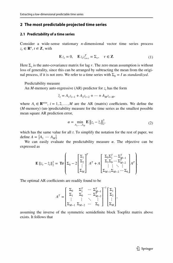
Consider a wide-sense stationary n-dimensional vector time series process zt ∈ �n , t ∈ � , with
Here Σ� is the auto-covariance matrix for lag � . The zero mean assumption is without loss of generality, since this can be arranged by subtracting the mean from the origi-nal process, if it is not zero. We refer to a time series with Σ0 = I as standardized.
Predictability measureAn M-memory auto-regressive (AR) predictor for zt has the form
where Ai ∈ �n×n , i = 1, 2,… ,M are the AR (matrix) coefficients. We define the (M-memory) (un-)predictability measure for the time series as the smallest possible mean square AR prediction error,
which has the same value for all t. To simplify the notation for the rest of paper, we define A =
[A1 ⋯ AM
].
We can easily evaluate the predictability measure � . The objective can be expressed as
The optimal AR coefficients are readily found to be
assuming the inverse of the symmetric semidefinite block Toeplitz matrix above exists. It follows that
(1)� zt = 0, � ztzTt+�
= Σ� , � ∈ �.
zt = A1zt−1 + A2zt−2 +⋯ + AMzt−M ,
(2)𝛼 = minA1,…,AM
� ‖‖zt − zt‖‖22,
� ‖zt − zt‖22 = ��
⎛⎜⎜⎜⎜⎝Σ0 − 2
⎡⎢⎢⎢⎣
Σ1
Σ2
⋮
ΣM
⎤⎥⎥⎥⎦
T
AT + A
⎡⎢⎢⎢⎣
Σ0ΣT1⋯ΣT
M−1
Σ1Σ0 ⋯ΣTM−2
⋮ ⋮ ⋱ ⋮
ΣM−1ΣM−2 ⋯Σ0
⎤⎥⎥⎥⎦AT
⎞⎟⎟⎟⎟⎠.
AT =
⎡⎢⎢⎢⎣
Σ0 ΣT1
⋯ ΣTM−1
Σ1 Σ0 ⋯ ΣTM−2
⋮ ⋮ ⋱ ⋮
ΣM−1 ΣM−2 ⋯ Σ0
⎤⎥⎥⎥⎦
−1 ⎡⎢⎢⎢⎣
Σ1
Σ2
⋮
ΣM
⎤⎥⎥⎥⎦,
Y. Dong et al.
1 3
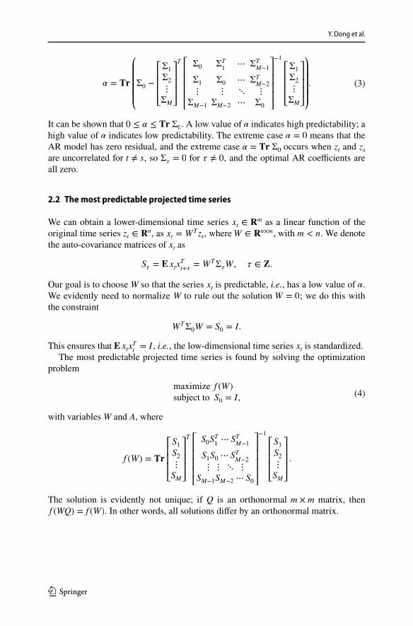
It can be shown that 0 ≤ � ≤ �� Σ0 . A low value of � indicates high predictability; a high value of � indicates low predictability. The extreme case � = 0 means that the AR model has zero residual, and the extreme case � = �� Σ0 occurs when zt and zs are uncorrelated for t ≠ s , so Σ� = 0 for � ≠ 0 , and the optimal AR coefficients are all zero.
2.2 The most predictable projected time series
We can obtain a lower-dimensional time series xt ∈ �m as a linear function of the original time series zt ∈ �n , as xt = WTzt , where W ∈ �n×m , with m < n . We denote the auto-covariance matrices of xt as
Our goal is to choose W so that the series xt is predictable, i.e., has a low value of � . We evidently need to normalize W to rule out the solution W = 0 ; we do this with the constraint
This ensures that � xtxTt= I , i.e., the low-dimensional time series xt is standardized.
The most predictable projected time series is found by solving the optimization problem
with variables W and A, where
The solution is evidently not unique; if Q is an orthonormal m × m matrix, then f (WQ) = f (W) . In other words, all solutions differ by an orthonormal matrix.
(3)� = ��
⎛⎜⎜⎜⎜⎝Σ0−
⎡⎢⎢⎢⎣
Σ1
Σ2
⋮
ΣM
⎤⎥⎥⎥⎦
T ⎡⎢⎢⎢⎢⎣
Σ0
ΣT
1⋯ ΣT
M−1
Σ1
Σ0
⋯ ΣT
M−2
⋮ ⋮ ⋱ ⋮
ΣM−1 Σ
M−2 ⋯ Σ0
⎤⎥⎥⎥⎥⎦
−1
⎡⎢⎢⎢⎣
Σ1
Σ2
⋮
ΣM
⎤⎥⎥⎥⎦
⎞⎟⎟⎟⎟⎠.
S� = � xtxTt+�
= WTΣ�W, � ∈ �.
WTΣ0W = S0 = I.
(4)maximize f (W)
subject to S0 = I,
f (W) = ��
⎡⎢⎢⎢⎣
S1
S2
⋮
SM
⎤⎥⎥⎥⎦
T ⎡⎢⎢⎢⎢⎣
S0ST1⋯ ST
M−1
S1S0⋯ ST
M−2
⋮ ⋮ ⋱ ⋮
SM−1SM−2 ⋯ S0
⎤⎥⎥⎥⎥⎦
−1
⎡⎢⎢⎢⎣
S1
S2
⋮
SM
⎤⎥⎥⎥⎦.
1 3
Extracting a low-dimensional predictable time series
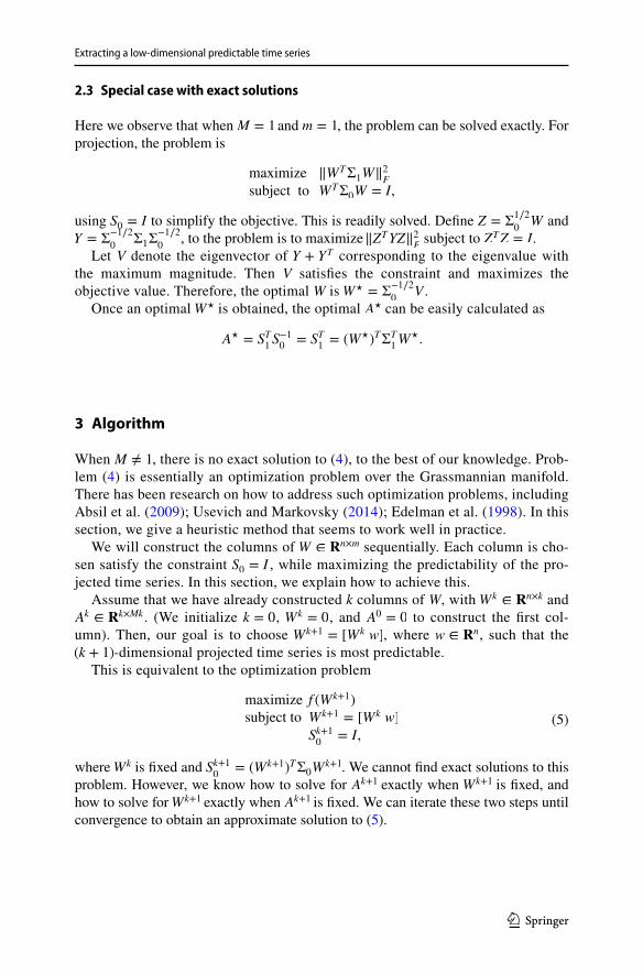
2.3 Special case with exact solutions
Here we observe that when M = 1 and m = 1 , the problem can be solved exactly. For projection, the problem is
using S0 = I to simplify the objective. This is readily solved. Define Z = Σ1∕2
0W and
Y = Σ−1∕2
0Σ1Σ
−1∕2
0 , to the problem is to maximize ‖ZTYZ‖2
F subject to ZTZ = I.
Let V denote the eigenvector of Y + YT corresponding to the eigenvalue with the maximum magnitude. Then V satisfies the constraint and maximizes the objective value. Therefore, the optimal W is W⋆ = Σ
−1∕2
0V .
Once an optimal W⋆ is obtained, the optimal A⋆ can be easily calculated as
3 Algorithm
When M ≠ 1 , there is no exact solution to (4), to the best of our knowledge. Prob-lem (4) is essentially an optimization problem over the Grassmannian manifold. There has been research on how to address such optimization problems, including Absil et al. (2009); Usevich and Markovsky (2014); Edelman et al. (1998). In this section, we give a heuristic method that seems to work well in practice.
We will construct the columns of W ∈ �n×m sequentially. Each column is cho-sen satisfy the constraint S0 = I , while maximizing the predictability of the pro-jected time series. In this section, we explain how to achieve this.
Assume that we have already constructed k columns of W, with Wk ∈ �n×k and Ak ∈ �k×Mk . (We initialize k = 0 , Wk = 0 , and A0 = 0 to construct the first col-umn). Then, our goal is to choose Wk+1 = [Wk w] , where w ∈ �n , such that the (k + 1)-dimensional projected time series is most predictable.
This is equivalent to the optimization problem
where Wk is fixed and Sk+10
= (Wk+1)TΣ0Wk+1 . We cannot find exact solutions to this
problem. However, we know how to solve for Ak+1 exactly when Wk+1 is fixed, and how to solve for Wk+1 exactly when Ak+1 is fixed. We can iterate these two steps until convergence to obtain an approximate solution to (5).
maximize ‖WTΣ1W‖2F
subject to WTΣ0W = I,
A⋆ = ST1S−10
= ST1= (W⋆)TΣT
1W⋆.
(5)maximize f (Wk+1)
subject to Wk+1 = [Wk w]
Sk+10
= I,
Y. Dong et al.
1 3
3.1 Solving for Ak+1 with fixed w
When w is fixed, we can solve for Ak+1 exactly. According to Sect. 2.1, when Wk+1 is known, the solution of Ak+1 is
where Sk+1�
= Wk+1,TΣ�Wk+1 , � ∈ �.
The time complexity for forming Sk+11
,… , Sk+1M
is O(M(k + 1)n2) . Once Sk+1�
, � = 1,… ,M are calculated, the time complexity for updating Ak+1 is dominated by the inversion step, which is O(M3(k + 1)3) . Therefore, the overall time complexity for updating Ak+1 is max
{O(M(k + 1)n2),O(M3(k + 1)3)
}.
3.2 Solving for w with fixed Ak+1
When Ak+1 is fixed, we can solve for Wk+1 exactly. With some derivations, the optimi-zation problem for w can be expressed as
where B ≻ 0 , and B, c are known. The derivation and expressions for B and c can be found in Appendix A. The solution of this problem can be obtained explicitly as follows.
Let U ∈ �n×(n−k) be the orthogonal complement of Σ1∕2
0Wk and UTU = I . Denote
the SVD decomposition of UTΣ−1∕2
0BΣ
−1∕2
0U as UTΣ
−1∕2
0BΣ
−1∕2
0U = VΛVT with
Λ = ����(�1,… , �n−k) , ( �1 ≤ �2 ⋯ ≤ �n−k ). Then, problem (6) can be transformed as
where � = [�1 �2 ⋯ �n−k] = VTUTΣ−1∕2
0c and w = Σ
−1∕2
0UVy . The solution to prob-
lem (7) has the form y = (Λ + �I)−1� where � can be obtained as the root of
that satisfies 𝜇 > −𝜆1.After � is found, the optimal w of problem (6) can be obtained as
Ak+1,T =
⎡⎢⎢⎢⎢⎣
Sk+10
Sk+1,T
1⋯ S
k+1,T
M−1
Sk+11
Sk+10
⋯ Sk+1,T
M−2
⋮ ⋮ ⋱ ⋮
Sk+1M−1
Sk+1M−2
⋯ Sk+10
⎤⎥⎥⎥⎥⎦
−1 ⎡⎢⎢⎢⎢⎣
Sk+11
Sk+12
⋮
Sk+1M
⎤⎥⎥⎥⎥⎦,
(6)minimize f (w) = wTBw − 2cTw
subject to Wk,TΣ0w = 0
wTΣ0w = 1,
(7)minimize f (z) = yTΛy − 2�Ty
subject to yTy = 1,
n−k∑i=1
�2i
(�i + �)2= 1
w⋆ = Σ−1∕2
0UV(Λ + 𝜇I)−1𝛽.
1 3
Extracting a low-dimensional predictable time series
According to the expressions of B and c in Appendix A, the time complexity for forming B and c is O(M2n2) . Once B and c are calculated, the time complexity for updating w is dominated by the SVD step, which is O(n3) . Therefore, the overall time complexity for updating w is max
{O(M2n2),O(n3)
}.
3.3 Complete algorithm
We have discussed algorithms to solve for Ak+1 when Wk+1 is fixed and to solve for Wk+1 = [Wk w] when Ak+1 is fixed. The complete procedure to con-struct the (k + 1)th column of W is to iterate these two steps until convergence. As discussed in Sects. 3.1 and 3.2, the time complexity for updating Ak+1 is max
{O(M(k + 1)n2),O(M3(k + 1)3)
} , and the time complexity for updating w is
max{O(M2n2),O(n3)
} . In practice, it is often the case that m ≪ n and M ≪ n . There-
fore, the overall time complexity at each iteration step is O(n3).Once Wk+1,Ak+1 are obtained, the same procedure can be applied to construct the
next column of W. The complete algorithm is given in Algorithm 1.
The heuristic method proposed has two advantages over directly solving the origi-nal problem (4). First, there is no uniqueness issue in this recursive method, because starting from the first column of W, each column of W is deterministic according to the optimization problem (6). Second, the iterative procedure gives an indication of the dimension of the predictable vector time series.
Let �k denote the predictability measure for the k dimensional projected time series, or the value of the objective function in (4) with optimal Wk and Ak . Then, when extracting the (k + 1) th scalar time series, we have the following upper bound for �k+1 of the (k + 1)-dimensional time series,
When the optimal �k+1 is very close to the upper bound �k + 1 , we can draw two conclusions. First, adding another scalar time series does not improve the prediction of the k dimensional vector time series. Second, no other self-predictable scalar time series can be extracted. These two facts suggest that all the predictable components in the time series data are already extracted and hence, we can stop the iteration procedure.
�k+1 ≤ �k + wTΣ0w = �k + 1.
Y. Dong et al.
1 3
4 Examples
In this section, we test our method by applying it to a synthesized high-dimensional time series dataset and a quarterly GDP growth dataset. In both examples, we dem-onstrate advantages of our proposed method over scalar time series AR fitting.
4.1 Simulation dataset
The proposed method is first tested on a synthesized dataset generated from the model
where
The matrix P ∈ �1000×3 is random matrix with orthonormal columns, Q ∈ �1000×1000 is a random orthonormal matrix, vt is i.i.d. N(0, I) and et is i.i.d N(0, 0.022I) . Σy is the empirical covariance matrix of yt , calculated as
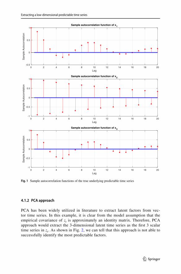
where T in the number of samples. In this example, 10,000 consecutive samples are generated from the model. Hence, T = 10, 000 . The sample autocorrelation func-tions of the true underlying predictable time series xt are plotted in Fig. 1. We can see that there are strong temporal dependence in xt.
4.1.1 Scalar AR approach
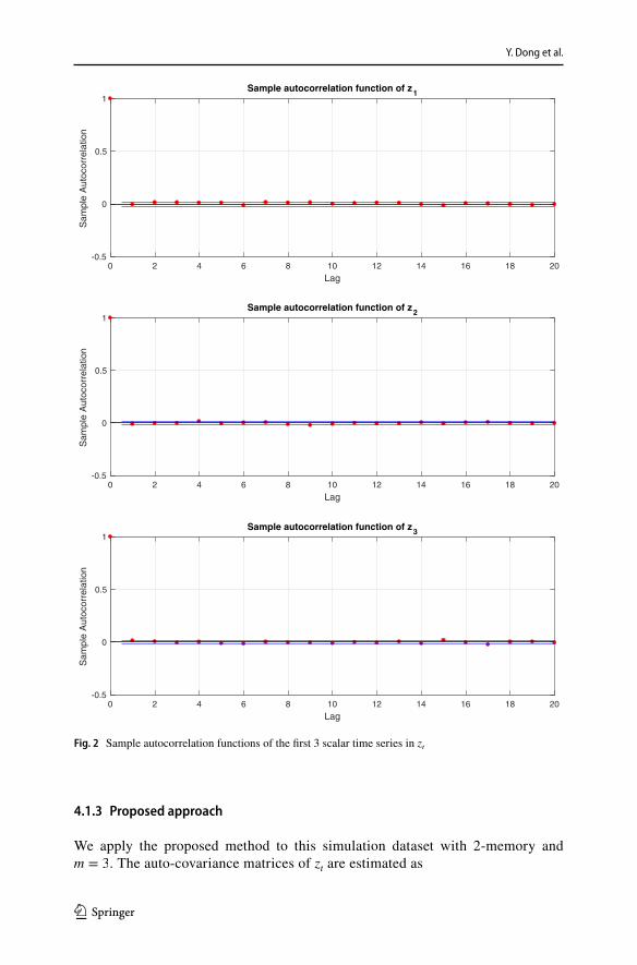
We first fit a 2-memory AR model to each scalar time series in zt to check the pre-dictability of each scalar time series. We use mean squared error (MSE) to evaluate the prediction performance of the fitted AR predictors. We find that, of all 1000 sca-lar time series, the minimal MSE is 0.9984 and the maximum MSE is 1.0000. Since each scalar time series has approximately mean 0 and variance 1, this indicates that 2-memory scalar AR fitting fails to extract any significant predictability information from the data. The autocorrelation functions of the first 3 scalar time series in zt are plotted in Fig. 2. It is quite clear that there are no significant temporal dependence that can be observed.
(8)xt = B1xt−1 + B2xt−2 + vt,
yt = Pxt + et,
zt = QΣ−1∕2y yt,
B1 =
⎡⎢⎢⎣
1.1241 0.3045 0.3806
0.3902 − 0.8169 − 0.3114
−0.7166 − 0.8630 1.0115
⎤⎥⎥⎦, B2 =
⎡⎢⎢⎣
−0.2482 0.3676 0.0328
−0.4240 0.1101 0.0267
0.6011 − 0.5975 − 0.3224
⎤⎥⎥⎦.
Σy =1
T
T∑t=1
ytyTt,
1 3
Extracting a low-dimensional predictable time series
4.1.2 PCA approach
PCA has been widely utilized in literature to extract latent factors from vec-tor time series. In this example, it is clear from the model assumption that the empirical covariance of zt is approximately an identity matrix. Therefore, PCA approach would extract the 3-dimensional latent time series as the first 3 scalar time series in zt . As shown in Fig. 2, we can tell that this approach is not able to successfully identify the most predictable factors.
0 2 4 6 8 10 12 14 16 18 20
Lag
-0.5
0
0.5
1
Sam
ple
Aut
ocor
rela
tion
Sample autocorrelation function of x1
0 2 4 6 8 10 12 14 16 18 20
Lag
-1
-0.5
0
0.5
1
Sam
ple
Aut
ocor
rela
tion
Sample autocorrelation function of x2
0 2 4 6 8 10 12 14 16 18 20
Lag
-1
-0.5
0
0.5
1
Sam
ple
Aut
ocor
rela
tion
Sample autocorrelation function of x3
Fig. 1 Sample autocorrelation functions of the true underlying predictable time series
Y. Dong et al.
1 3
4.1.3 Proposed approach
We apply the proposed method to this simulation dataset with 2-memory and m = 3 . The auto-covariance matrices of zt are estimated as
0 2 4 6 8 10 12 14 16 18 20
Lag
-0.5
0
0.5
1
Sam
ple
Aut
ocor
rela
tion
Sample autocorrelation function of z1
0 2 4 6 8 10 12 14 16 18 20
Lag
-0.5
0
0.5
1
Sam
ple
Aut
ocor
rela
tion
Sample autocorrelation function of z2
0 2 4 6 8 10 12 14 16 18 20
Lag
-0.5
0
0.5
1
Sam
ple
Aut
ocor
rela
tion
Sample autocorrelation function of z3
Fig. 2 Sample autocorrelation functions of the first 3 scalar time series in zt
1 3
Extracting a low-dimensional predictable time series
and
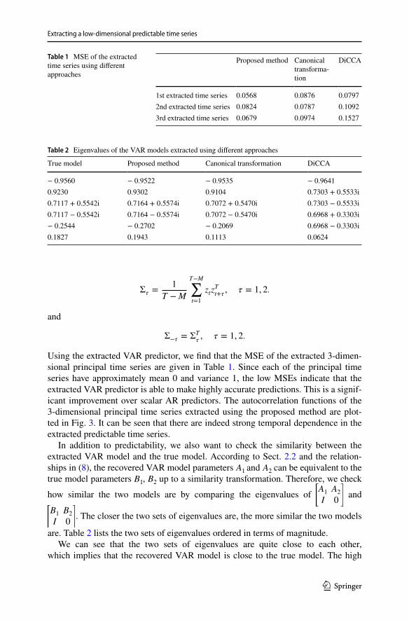
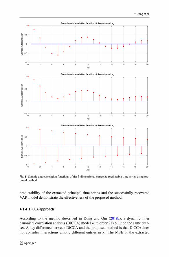
Using the extracted VAR predictor, we find that the MSE of the extracted 3-dimen-sional principal time series are given in Table 1. Since each of the principal time series have approximately mean 0 and variance 1, the low MSEs indicate that the extracted VAR predictor is able to make highly accurate predictions. This is a signif-icant improvement over scalar AR predictors. The autocorrelation functions of the 3-dimensional principal time series extracted using the proposed method are plot-ted in Fig. 3. It can be seen that there are indeed strong temporal dependence in the extracted predictable time series.
In addition to predictability, we also want to check the similarity between the extracted VAR model and the true model. According to Sect. 2.2 and the relation-ships in (8), the recovered VAR model parameters A1 and A2 can be equivalent to the true model parameters B1 , B2 up to a similarity transformation. Therefore, we check
how similar the two models are by comparing the eigenvalues of [A1 A2
I 0
] and [
B1 B2
I 0
] . The closer the two sets of eigenvalues are, the more similar the two models
are. Table 2 lists the two sets of eigenvalues ordered in terms of magnitude.We can see that the two sets of eigenvalues are quite close to each other,
which implies that the recovered VAR model is close to the true model. The high
Σ� =1
T −M
T−M∑t=1
ztzTt+�
, � = 1, 2.
Σ−� = ΣT�, � = 1, 2.
Table 1 MSE of the extracted time series using different approaches
Proposed method Canonical transforma-tion
DiCCA
1st extracted time series 0.0568 0.0876 0.07972nd extracted time series 0.0824 0.0787 0.10923rd extracted time series 0.0679 0.0974 0.1527
Table 2 Eigenvalues of the VAR models extracted using different approaches
True model Proposed method Canonical transformation DiCCA
− 0.9560 − 0.9522 − 0.9535 − 0.96410.9230 0.9302 0.9104 0.7303 + 0.5533i0.7117 + 0.5542i 0.7164 + 0.5574i 0.7072 + 0.5470i 0.7303 − 0.5533i0.7117 − 0.5542i 0.7164 − 0.5574i 0.7072 − 0.5470i 0.6968 + 0.3303i− 0.2544 − 0.2702 − 0.2069 0.6968 − 0.3303i0.1827 0.1943 0.1113 0.0624
Y. Dong et al.
1 3
predictability of the extracted principal time series and the successfully recovered VAR model demonstrate the effectiveness of the proposed method.
4.1.4 DiCCA approach
According to the method described in Dong and Qin (2018a), a dynamic-inner canonical correlation analysis (DiCCA) model with order 2 is built on the same data-set. A key difference between DiCCA and the proposed method is that DiCCA does not consider interactions among different entries in xt . The MSE of the extracted
0 2 4 6 8 10 12 14 16 18 20
Lag
-1
-0.5
0
0.5
1
Sam
ple
Aut
ocor
rela
tion
Sample autocorrelation function of the extracted x1
0 2 4 6 8 10 12 14 16 18 20
Lag
-0.5
0
0.5
1
Sam
ple
Aut
ocor
rela
tion
Sample autocorrelation function of the extracted x2
0 2 4 6 8 10 12 14 16 18 20
Lag
-1
-0.5
0
0.5
1
Sam
ple
Aut
ocor
rela
tion
Sample autocorrelation function of the extracted x3
Fig. 3 Sample autocorrelation functions of the 3-dimensional extracted predictable time series using pro-posed method
1 3
Extracting a low-dimensional predictable time series
3-dimensional time series are listed in Table 1, and eigenvalues of the recovered VAR model are given in Table 2. Since DiCCA does not consider the predictabili-ties among different entires in xt , it has higher MSE values and large differences from the true eigenvalues.
4.1.5 Canonical transformation approach
According to the method described in Box and Tiao (1977), a full-dimensional VAR model with 2-memory is fit to zt first, and the covariance matrix Σ(z) of the predic-tion zt is calculated. The linear transformation matrix W1 is selected as the eigen-vectors corresponding to the largest magnitude eigenvalues of matrix Σ−1
0Σ(z) . The
MSE values of the extracted 3-dimensional latent time series are listed in Table 1 as well.
In fact, many methods that extract lower-dimensional predictable time series involve fitting a high-dimensional VAR model (which can be very time consuming when n and M are large), and do not consider the prediction models for the lower-dimensional predictable time series in the objective functions. An AR model is often fit subsequently after extracting the lower-dimensional predictable time series for prediction purposes. In order to examine how closely this method recovers the underlying model structure, a VAR model with 2-memory is fit to WT
1zt , and the
eigenvalues are listed in Table 2. Compare to the proposed method, it recovers the small magnitude eigenvalues less accurately than the proposed method.
4.1.6 PFA approach and reduced rank AR approach
The predictable factor analysis (PFA) method developed in Richthofer and Wiskott (2015) without nonlinear expansion and regularization was tested, as well as the reduced rank AR approach discussed in Velu et al. (1986). In fact, we can show that without special treatment, these two approaches are equivalent to the canonical transformation method in Box and Tiao (1977), and the results are the same as the results of the canonical transformation method.
4.2 GDP dataset
This dataset is composed of seasonally adjusted quarterly GDP growth data of 17 countries from 1961-Q2 to 2017-Q3. The 17 countries are selected based on the largest GDP countries according to the world bank data in 2016 with complete GDP growth records from 1961-Q2 to 2017-Q3, and this data is downloaded from https:// stats. oecd. org/ index. aspx? query id= 350#. The 17 countries are United States, Japan, United Kingdom, France, Italy, Canada, South Korea, Australia, Spain, Mexico, Netherlands, Switzerland, Germany, Sweden, Belgium, Austria, and Norway.
Two approaches are applied to the first 135 samples from 1961-Q2 to 1994-Q4. The first approach is to fit a single variable AR model to each country’s GDP data. The sec-ond approach is to use the proposed method in this work to extract the most predictable principal time series. For each approach, the 135 samples are preprocessed such that
Y. Dong et al.
1 3
each variable has zero mean and unit variance, and an AR model with 1-memory is fit-ted to the preprocessed data.
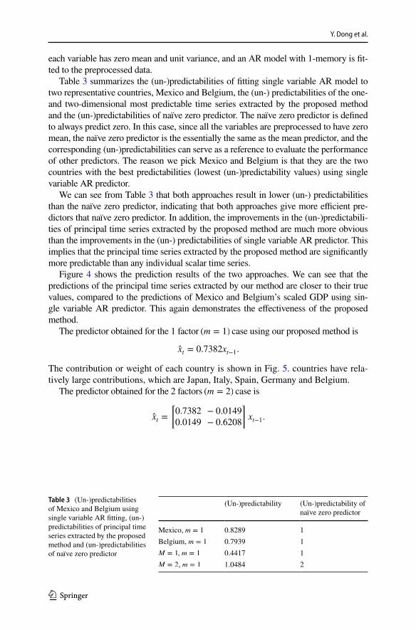
Table 3 summarizes the (un-)predictabilities of fitting single variable AR model to two representative countries, Mexico and Belgium, the (un-) predictabilities of the one- and two-dimensional most predictable time series extracted by the proposed method and the (un-)predictabilities of naïve zero predictor. The naïve zero predictor is defined to always predict zero. In this case, since all the variables are preprocessed to have zero mean, the naïve zero predictor is the essentially the same as the mean predictor, and the corresponding (un-)predictabilities can serve as a reference to evaluate the performance of other predictors. The reason we pick Mexico and Belgium is that they are the two countries with the best predictabilities (lowest (un-)predictability values) using single variable AR predictor.
We can see from Table 3 that both approaches result in lower (un-) predictabilities than the naïve zero predictor, indicating that both approaches give more efficient pre-dictors that naïve zero predictor. In addition, the improvements in the (un-)predictabili-ties of principal time series extracted by the proposed method are much more obvious than the improvements in the (un-) predictabilities of single variable AR predictor. This implies that the principal time series extracted by the proposed method are significantly more predictable than any individual scalar time series.
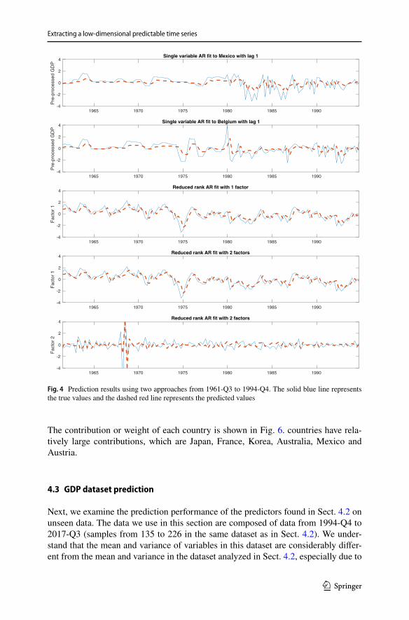
Figure 4 shows the prediction results of the two approaches. We can see that the predictions of the principal time series extracted by our method are closer to their true values, compared to the predictions of Mexico and Belgium’s scaled GDP using sin-gle variable AR predictor. This again demonstrates the effectiveness of the proposed method.
The predictor obtained for the 1 factor (m = 1) case using our proposed method is
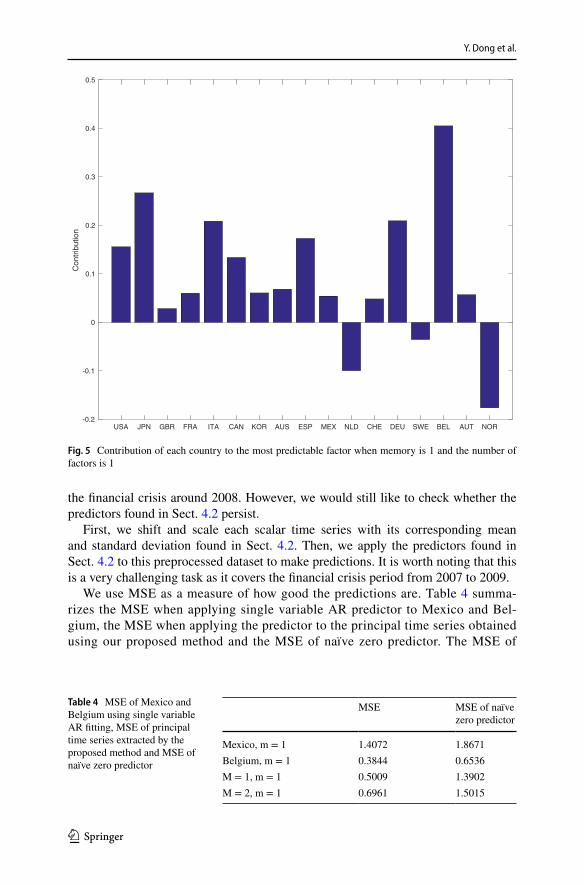
The contribution or weight of each country is shown in Fig. 5. countries have rela-tively large contributions, which are Japan, Italy, Spain, Germany and Belgium.
The predictor obtained for the 2 factors (m = 2) case is
xt = 0.7382xt−1.
xt =
[0.7382 − 0.0149
0.0149 − 0.6208
]xt−1.
Table 3 (Un-)predictabilities of Mexico and Belgium using single variable AR fitting, (un-)predictabilities of principal time series extracted by the proposed method and (un-)predictabilities of naïve zero predictor
(Un-)predictability (Un-)predictability of naïve zero predictor
Mexico, m = 1 0.8289 1Belgium, m = 1 0.7939 1M = 1 , m = 1 0.4417 1M = 2 , m = 1 1.0484 2
1 3
Extracting a low-dimensional predictable time series
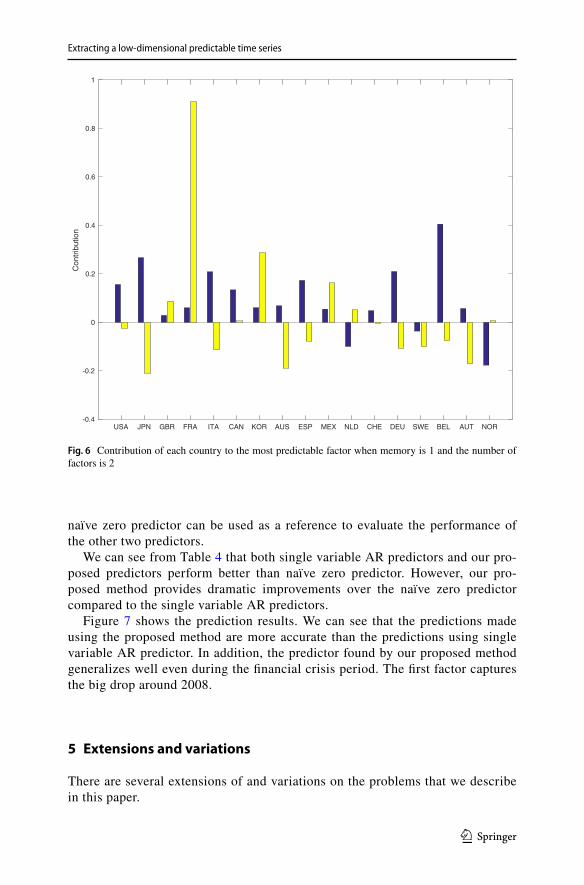
The contribution or weight of each country is shown in Fig. 6. countries have rela-tively large contributions, which are Japan, France, Korea, Australia, Mexico and Austria.
4.3 GDP dataset prediction
Next, we examine the prediction performance of the predictors found in Sect. 4.2 on unseen data. The data we use in this section are composed of data from 1994-Q4 to 2017-Q3 (samples from 135 to 226 in the same dataset as in Sect. 4.2). We under-stand that the mean and variance of variables in this dataset are considerably differ-ent from the mean and variance in the dataset analyzed in Sect. 4.2, especially due to
1965 1970 1975 1980 1985 1990-4
-2
0
2
4
Pre
-pro
cess
ed G
DP
Single variable AR fit to Mexico with lag 1
1965 1970 1975 1980 1985 1990-4
-2
0
2
4
Pre
-pro
cess
ed G
DP
Single variable AR fit to Belgium with lag 1
1965 1970 1975 1980 1985 1990-4
-2
0
2
4
Fac
tor
1
Reduced rank AR fit with 1 factor
1965 1970 1975 1980 1985 1990-4
-2
0
2
4
Fac
tor
1
Reduced rank AR fit with 2 factors
1965 1970 1975 1980 1985 1990-4
-2
0
2
4
Fac
tor
2
Reduced rank AR fit with 2 factors
Fig. 4 Prediction results using two approaches from 1961-Q3 to 1994-Q4. The solid blue line represents the true values and the dashed red line represents the predicted values
Y. Dong et al.
1 3
the financial crisis around 2008. However, we would still like to check whether the predictors found in Sect. 4.2 persist.
First, we shift and scale each scalar time series with its corresponding mean and standard deviation found in Sect. 4.2. Then, we apply the predictors found in Sect. 4.2 to this preprocessed dataset to make predictions. It is worth noting that this is a very challenging task as it covers the financial crisis period from 2007 to 2009.
We use MSE as a measure of how good the predictions are. Table 4 summa-rizes the MSE when applying single variable AR predictor to Mexico and Bel-gium, the MSE when applying the predictor to the principal time series obtained using our proposed method and the MSE of naïve zero predictor. The MSE of
USA JPN GBR FRA ITA CAN KOR AUS ESP MEX NLD CHE DEU SWE BEL AUT NOR-0.2
-0.1
0
0.1
0.2
0.3
0.4
0.5C
ontr
ibut
ion
Fig. 5 Contribution of each country to the most predictable factor when memory is 1 and the number of factors is 1
Table 4 MSE of Mexico and Belgium using single variable AR fitting, MSE of principal time series extracted by the proposed method and MSE of naïve zero predictor
MSE MSE of naïve zero predictor
Mexico, m = 1 1.4072 1.8671Belgium, m = 1 0.3844 0.6536M = 1, m = 1 0.5009 1.3902M = 2, m = 1 0.6961 1.5015
1 3
Extracting a low-dimensional predictable time series
naïve zero predictor can be used as a reference to evaluate the performance of the other two predictors.
We can see from Table 4 that both single variable AR predictors and our pro-posed predictors perform better than naïve zero predictor. However, our pro-posed method provides dramatic improvements over the naïve zero predictor compared to the single variable AR predictors.
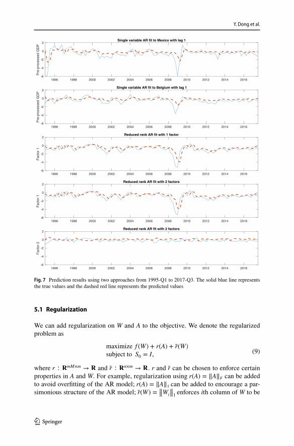
Figure 7 shows the prediction results. We can see that the predictions made using the proposed method are more accurate than the predictions using single variable AR predictor. In addition, the predictor found by our proposed method generalizes well even during the financial crisis period. The first factor captures the big drop around 2008.
5 Extensions and variations
There are several extensions of and variations on the problems that we describe in this paper.
USA JPN GBR FRA ITA CAN KOR AUS ESP MEX NLD CHE DEU SWE BEL AUT NOR-0.4
-0.2
0
0.2
0.4
0.6
0.8
1C
ontr
ibut
ion
Fig. 6 Contribution of each country to the most predictable factor when memory is 1 and the number of factors is 2
Y. Dong et al.
1 3
5.1 Regularization
We can add regularization on W and A to the objective. We denote the regularized problem as
where r ∶ �mM×m→ � and r ∶ �n×m
→ � . r and r can be chosen to enforce certain properties in A and W. For example, regularization using r(A) = ‖A‖F can be added to avoid overfitting of the AR model; r(A) = ‖A‖1 can be added to encourage a par-simonious structure of the AR model; r(W) = ‖‖Wi
‖‖1 enforces ith column of W to be
(9)maximize f (W) + r(A) + r(W)
subject to S0 = I,
1996 1998 2000 2002 2004 2006 2008 2010 2012 2014 2016-6
-4
-2
0
2
Pre
-pro
cess
ed G
DP
Single variable AR fit to Mexico with lag 1
1996 1998 2000 2002 2004 2006 2008 2010 2012 2014 2016-6
-4
-2
0
2
Pre
-pro
cess
ed G
DP
Single variable AR fit to Belgium with lag 1
1996 1998 2000 2002 2004 2006 2008 2010 2012 2014 2016-6
-4
-2
0
2
Fac
tor
1
Reduced rank AR fit with 1 factor
1996 1998 2000 2002 2004 2006 2008 2010 2012 2014 2016-6
-4
-2
0
2
Fac
tor
1
Reduced rank AR fit with 2 factors
1996 1998 2000 2002 2004 2006 2008 2010 2012 2014 2016-6
-4
-2
0
2
Fac
tor
2
Reduced rank AR fit with 2 factors
Fig. 7 Prediction results using two approaches from 1995-Q1 to 2017-Q3. The solid blue line represents the true values and the dashed red line represents the predicted values

1 3
Extracting a low-dimensional predictable time series
sparse, such that the ith most predictable time series only depends on a few entries in the high dimensional time series.
5.2 Low rank structure
In many cases, high dimensional time series have low rank structure. We can use this low rank structure to reduce the computational complexity of our problem. When the high dimensional time series has low rank structure, the covariance matrix Σ0 has many eigenvalues close 0. Let U denote the collections of all the eigenvectors of Σ0 corresponding to the significantly non-zero eigenvalues, then original inputs Σ� , � = 0, 1,… ,M can be approximately transformed into Φ� , � = 0, 1,… ,M , where Φ𝜏 = UTΣ𝜏U . Since the dimension of Φ� is much lower than the dimension of Σ� , by working with the new input series Φ� , the computational complexity reduces signifi-cantly. Let W� and A� denote the solutions with the new inputs Φ� , then the solutions with the original inputs Σ� can be obtained as
5.3 Filtering
As an extension of the projection method, we can consider extracting a lower-dimen-sional time series xt using a finite impulse response (FIR) filter with length L:
where W1,… ,WL ∈ �n×m are the filter coefficients. For L = 1 , this reduces to the projection problem (4). We can write this as
where
Define the following auto-covariance matrices of
⎡⎢⎢⎢⎣
ztzt−1⋮
zt−L+1
⎤⎥⎥⎥⎦:
W = UW𝜙, A = A𝜙.
xt = WT1zt +WT
2zt−1 +⋯ +WT
Lzt−L+1, t ∈ �,
xt = WT
⎡⎢⎢⎢⎣
ztzt−1⋮
zt−L+1
⎤⎥⎥⎥⎦, t ∈ �,
W =
⎡⎢⎢⎢⎣
W1
W2
⋮
WL
⎤⎥⎥⎥⎦.
Y. Dong et al.
1 3
The goal is to choose W so that the series xt is most predictable by an M-memory AR predictor. Similar to the projection problem, we add the constraint S0 = WTΩ0W = I to rule out the trivial W = 0 case. This also ensures that the low-dimensional time series xt is standardized.
6 Related work
The general problem of extracting low-dimensional latent variables from high-dimensional time series has been studied for decades in many different research fields from control systems, signal processing, to economics. Many methods have been developed, and here we survey a subset of representative methods that are closely related to the proposed method.
6.1 Extracting predictable latent variables
The extraction of predictable latent variables can be traced back to the work Box and Tiao (1977), where canonical transformation is proposed to extract the lower dimensional components ordered from least to most predictable. Mathematically, the transformation matrix W in Box and Tiao (1977) is selected as the eigenvectors corresponding to the m largest eigenvalues in Σ−1
0Σ(z) , where Σ(z) = � zt z
Tt , and zt
is the one-step ahead prediction of zt found in (2). It is clear that the method in Box and Tiao (1977) is different from the proposed method unless M = 1 and m = 1.
Later in Pena and Box (1987), the zt vector is decomposed into one component that contains factors mixed up with noise, where the transformation matrix W is obtained by analyzing the eigenstructure of the VAR model coefficients of zt , and one component contains white noise.
The slow feature analysis (SFA) method proposed in Wiskott and Sejnowski (2002) aims to extract a lower-dimensional “slowly varying” time series. Without nonlinear expansion, SFA can be treated as a special case of the proposed method if we restrict M = 1 and A1 = I . Even though “slowly varying” time series are predict-able, predictable time series do not necessarily have slow variations. To deal with this, the later work Richthofer and Wiskott (2015) proposed a more general predict-able feature analysis (PFA) approach to extract lower-dimensional predictable time series. In PFA method, the selection of the transformation matrix W involves an
Ω0= �
⎡⎢⎢⎢⎣
ztzt−1⋮
zt−L+1
⎤⎥⎥⎥⎦
⎡⎢⎢⎢⎣
ztzt−1⋮
zt−L+1
⎤⎥⎥⎥⎦
T
=
⎡⎢⎢⎢⎢⎣
Σ0ΣT1⋯ΣT
L−1
Σ1Σ0⋯ΣT
L−2
⋮ ⋮ ⋱ ⋮
ΣL−1ΣL−2 ⋯Σ0
⎤⎥⎥⎥⎥⎦,
Ω1= �
⎡⎢⎢⎢⎣
ztzt−1⋮
zt−L+1
⎤⎥⎥⎥⎦
⎡⎢⎢⎢⎣
zt+1zt⋮
zt−L+2
⎤⎥⎥⎥⎦
T
=
⎡⎢⎢⎢⎢⎣
Σ1Σ0⋯ΣT
L−2
Σ2Σ1⋯ΣT
L−3
⋮ ⋮ ⋱ ⋮
ΣLΣL−1 ⋯Σ1
⎤⎥⎥⎥⎥⎦.
1 3
Extracting a low-dimensional predictable time series
eigen-decomposition of �(zt − zt)(zt − zt)T . As we can see, the PFA method is in
fact closely related to the method in Box and Tiao (1977), and is only equivalent to the proposed method when M = 1 and m = 1.
In all the above mentioned methods except SFA, a VAR model needs to be fit for the original high-dimensional time series. There have also been methods developed that do not involve fitting a high-dimensional VAR model. For example, in Dong and Qin (2018b, 2018a), dynamic-inner principal component analysis (DiPCA) and DiCCA are developed to extract a lower-dimensional most predictable latent varia-bles. In both methods, the columns of W are extracted sequentially, with a scalar AR predictor for each entry in xt . DiPCA extracts each entry in xt such that it has maxi-mal covariance between its predicted value using an AR predictor, while DiCCA maximizes the correlation. In fact, it can be shown that DiCCA is a special case of the proposed method where A1,A2,… ,AM are diagonal matrices.
Instead of using expected mean squared error as a predictability measure, there have been methods developed using different predictability measures. For example, forecastable component analysis (ForeCA) proposed in Goerg (2013) utilizes the differential entropy as the predictability (forecastability) measure, which yields the lower bound of the expected squared loss of any estimator. Graph-based predict-able feature analysis (GPFA) in Weghenkel et al. (2017) maximizes a predictability measure defined in terms of graph embedding. Dynamical component analysis in Clark et al. (2019) uses mutual information between the past and future data. The method developed in Stone (2001) proposed to use a measure of temporal predict-ability for blind source separation. In atmospheric, optimal persistence analysis (OPA) maximizes the decorrelation time (DelSole 2001), and average predictabil-ity time decomposition (APTD) maximizes the average predictability time (DelSole and Tippett 2009a, b).
6.2 Factor models
This work is also closely related to the extensively studied factor models in econo-metrics. Here we analyze some representative methods and compare them with the proposed method. The early work Brillinger (1981) is a frequency domain approach that extracts dynamic principal components (DPC) as linear combinations of the past and future observations to minimize the mean squared reconstruction error of the original high-dimensional time series. Similar structure exists in Peña and Yohai (2016), which is a time domain approach that uses non-causal models. In the later work Peña et al. (2019), a causal model is utilized to extract one-sided dynamic prin-cipal components (ODPC) as linear combinations of the current and past values of the series that minimize the reconstruction mean squared error. All of these methods extract latent factors differently from the proposed method, where the extraction of xt only depends on the current data. In addition, these methods extract latent factors by minimizing the mean squared reconstruction error, while the proposed method minimizes the mean squared prediction error.
In Lam and Yao (2012); Lam et al. (2011), for standardized high-dimensional time series, W is selected as the eigenvectors corresponding to the largest m
Y. Dong et al.
1 3
eigenvalues in ∑M
i=1ΣTiΣi . In Pan and Yao (2008), the latent factors are identified
via expanding the white noise space step by step. Compare to the proposed method, these methods provide little characterization on the lower-dimensional xt . To make predictions on xt , Lam et al. (2011) suggest to subsequently build an AR predictor. However, in the proposed method, the extraction and prediction of xt are achieved simultaneously by solving one optimization problem. A lot of the above analysis were also given in Qin et al. (2020), where Lam and Yao (2012) is linked to sub-space identification. Refer to Stock and Watson (2006), Stock and Watson (2011), Forni et al. (2000), Amengual and Watson (2007), Bai and Ng (2007) for more gen-eral discussions on factor models.
6.3 Reduced rank time series
Another related work is reduced rank time series modeling. Early work such as Rein-sel (1983), Velu et al. (1986), Ahn and Reinsel (1988), Wang and Bessler (2004) fit AR models to the vector time series with reduced rank coefficients. Later the reduced rank time series models have been generalized into the structured AR mod-eling problem (Basu et al. 2019; Alquier et al. 2020; Melnyk and Banerjee 2016; Barratt et al. 2021), where regularization terms on the AR model coefficients are imposed to encourage certain structures, such as low rank and sparsity. In summary, most of these papers focus on a parsimonious parametrization on the vector time series models, rather than extracting low-dimensional predictable time series.
6.4 State space models
The proposed method also has connections with state space models. There have been many ways to fit a state space model to vector time series, such as expectation-maximization (EM) (Shumway and Stoffer 1982), and N4SID (Moonen et al. 1989; Van Overschee and De Moor 1993) and CVA approach (Larimore 1983). In state space models, there have been methods developed to encourage sparse or low rank structures on the state transition matrix, such as She et al. (2018), Chen et al. (2017). Instead of adding regularizations on the state transition matrix, Angelosante et al. (2009), Charles et al. (2011) directly regularize the latent state to be sparse or low rank. In addition, there have been approaches that consider more general settings. For example, Lin and Michailidis (2020), Kost et al. (2018) consider the identifica-tion of linear dynamical systems with serially correlated output noise components. In the work of Qin et al. (2020), state space models are also compared with latent variable models, and it pointed out that subspace identification does not naturally yield reduced dimensional models.
In summary, the key difference between the proposed method and many of the existing methods is that first, it extracts low-dimensional predictable time series without fitting a full-dimensional VAR model; second, the extraction of principal
1 3
Extracting a low-dimensional predictable time series
time series and the VAR modeling of the principal time series are achieved simulta-neously by solving the optimization problem.
7 Conclusion
In this paper we have described a new method to extract a low-dimensional most predictable time series from high-dimensional time series, in the sense that an auto-regressive model achieves minimum prediction error. The method is heuristic, since the algorithm does not guarantee globally optimal. Numerical examples suggest, however, that the method works very well in practice.
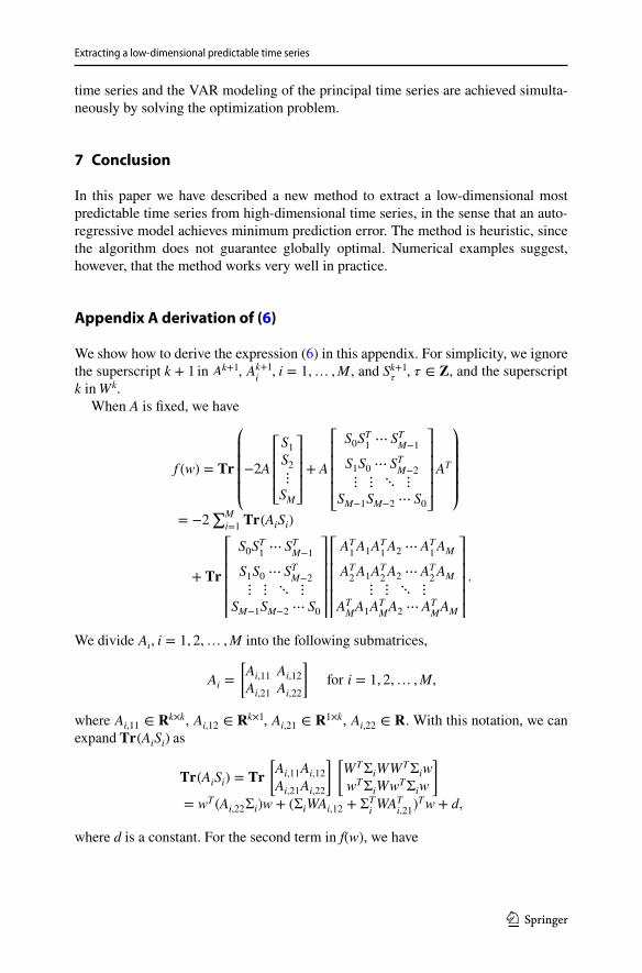
Appendix A derivation of (6)
We show how to derive the expression (6) in this appendix. For simplicity, we ignore the superscript k + 1 in Ak+1 , Ak+1
i , i = 1,… ,M , and Sk+1
� , � ∈ � , and the superscript
k in Wk.When A is fixed, we have
We divide Ai , i = 1, 2,… ,M into the following submatrices,
where Ai,11 ∈ �k×k , Ai,12 ∈ �k×1 , Ai,21 ∈ �1×k , Ai,22 ∈ � . With this notation, we can expand ��(AiSi) as
where d is a constant. For the second term in f(w), we have
f (w) = ��
⎛⎜⎜⎜⎜⎝−2A
⎡⎢⎢⎢⎣
S1
S2
⋮
SM
⎤⎥⎥⎥⎦+ A
⎡⎢⎢⎢⎢⎣
S0ST1⋯ ST
M−1
S1S0⋯ ST
M−2
⋮ ⋮ ⋱ ⋮
SM−1SM−2 ⋯ S0
⎤⎥⎥⎥⎥⎦AT
⎞⎟⎟⎟⎟⎠
= −2∑M
i=1��(AiSi)
+ ��
⎡⎢⎢⎢⎢⎣
S0ST1⋯ ST
M−1
S1S0⋯ ST
M−2
⋮ ⋮ ⋱ ⋮
SM−1SM−2 ⋯ S0
⎤⎥⎥⎥⎥⎦
⎡⎢⎢⎢⎢⎣
AT1A1AT1A2⋯AT
1AM
AT2A1AT2A2⋯AT
2AM
⋮ ⋮ ⋱ ⋮
ATMA1ATMA2⋯AT
MAM
⎤⎥⎥⎥⎥⎦.
Ai =
[Ai,11 Ai,12
Ai,21 Ai,22
]for i = 1, 2,… ,M,
��(AiSi) = ��
[Ai,11Ai,12
Ai,21Ai,22
] [WTΣiWWTΣiw
wTΣiWwTΣiw
]
= wT (Ai,22Σi)w + (ΣiWAi,12 + ΣTiWAT
i,21)Tw + d,
Y. Dong et al.
1 3
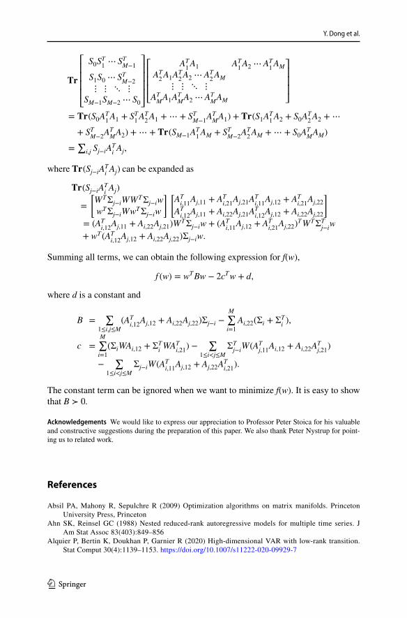
where ��(Sj−iATiAj) can be expanded as
Summing all terms, we can obtain the following expression for f(w),
where d is a constant and
The constant term can be ignored when we want to minimize f(w). It is easy to show that B ≻ 0.
Acknowledgements We would like to express our appreciation to Professor Peter Stoica for his valuable and constructive suggestions during the preparation of this paper. We also thank Peter Nystrup for point-ing us to related work.
References
Absil PA, Mahony R, Sepulchre R (2009) Optimization algorithms on matrix manifolds. Princeton University Press, Princeton
Ahn SK, Reinsel GC (1988) Nested reduced-rank autoregressive models for multiple time series. J Am Stat Assoc 83(403):849–856
Alquier P, Bertin K, Doukhan P, Garnier R (2020) High-dimensional VAR with low-rank transition. Stat Comput 30(4):1139–1153. https:// doi. org/ 10. 1007/ s11222- 020- 09929-7
��
⎡⎢⎢⎢⎢⎣
S0ST1⋯ ST
M−1
S1S0⋯ ST
M−2
⋮ ⋮ ⋱ ⋮
SM−1SM−2 ⋯ S0
⎤⎥⎥⎥⎥⎦
⎡⎢⎢⎢⎣
AT1A1
AT1A2⋯AT
1AM
AT2A1AT2A2⋯AT
2AM
⋮ ⋮ ⋱ ⋮
ATMA1ATMA2⋯AT
MAM
⎤⎥⎥⎥⎦
= ��(S0AT1A1+ ST
1AT2A1+⋯ + ST
M−1ATMA1) + ��(S
1AT1A2+ S
0AT2A2+⋯
+ STM−2
ATMA2) +⋯ + ��(SM−1A
T1AM + ST
M−2AT2AM +⋯ + S
0ATMAM)
=∑
i,j Sj−iATiAj,
��(Sj−iATiAj)
=
[WTΣj−iWWTΣj−iw
wTΣj−iWwTΣj−iw
] [ATi,11
Aj,11 + ATi,21
Aj,21ATi,11
Aj,12 + ATi,21
Aj,22
ATi,12
Aj,11 + Ai,22Aj,21ATi,12
Aj,12 + Ai,22Aj,22
]
= (ATi,12
Aj,11 + Ai,22Aj,21)WTΣj−iw + (AT
i,11Aj,12 + AT
i,21Aj,22)
TWTΣTj−iw
+ wT (ATi,12
Aj,12 + Ai,22Aj,22)Σj−iw.
f (w) = wTBw − 2cTw + d,
B =∑
1≤i,j≤M
(ATi,12
Aj,12 + Ai,22Aj,22)Σj−i −M∑i=1
Ai,22(Σi + ΣTi),
c =M∑i=1
(ΣiWAi,12 + ΣTiWAT
i,21) −
∑1≤i<j≤M
ΣTj−iW(AT
j,11Ai,12 + Ai,22A
Tj,21
)
−∑
1≤i<j≤M
Σj−iW(ATi,11
Aj,12 + Aj,22ATi,21
).

1 3
Extracting a low-dimensional predictable time series
Amengual D, Watson MW (2007) Consistent estimation of the number of dynamic factors in a large N and T panel. J Bus Econ Stat 25(1):91–96
Angelosante D, Roumeliotis SI, Giannakis GB (2009) Lasso-Kalman smoother for tracking sparse sig-nals. In: 2009 Conference record of the forty-third asilomar conference on signals, systems and computers, IEEE, pp 181–185
Bai J, Ng S (2007) Determining the number of primitive shocks in factor models. J Bus Econ Stat 25(1):52–60
Bai J, Ng S (2008) Large dimensional factor analysis. Found Trend Reg Econ 3(2):89–163Barratt S, Dong Y, Boyd S (2021) Low rank forecasting. arXiv preprint arXiv: 21011 2414Basu S, Li X, Michailidis G (2019) Low rank and structured modeling of high-dimensional vector autore-
gressions. IEEE Trans Sig Process 67(5):1207–1222Box GE, Tiao GC (1977) A canonical analysis of multiple time series. Biometrika 64(2):355–365Brillinger DR (1981) Time series: data analysis and theory, Expanded. Holden-Day Inc, New YorkCharles A, Asif MS, Romberg J, Rozell C (2011) Sparsity penalties in dynamical system estimation. In:
2011 45th annual conference on information sciences and systems, IEEE, pp 1–6Chen S, Liu K, Yang Y, Xu Y, Lee S, Lindquist M, Caffo BS, Vogelstein JT (2017) An M-estimator for
reduced-rank system identification. Pattern Recognit Lett 86:76–81Choi I (2012) Efficient estimation of factor models. Econ Theory 28(2):274–308Clark DG, Livezey JA, Bouchard KE (2019) Unsupervised discovery of temporal structure in noisy data
with dynamical components analysis. arXiv preprint arXiv: 19050 9944Connor G, Korajczyk RA (1986) Performance measurement with the arbitrage pricing theory: a new
framework for analysis. J Financ Econ 15(3):373–394DelSole T (2001) Optimally persistent patterns in time-varying fields. J Atmosph Sci 58(11):1341–1356DelSole T, Tippett MK (2009a) Average predictability time: part i–theory. J Atmosph Sci
66(5):1172–1187DelSole T, Tippett MK (2009b) Average predictability time: part ii–Seamless diagnoses of predictability
on multiple time scales. J Atmosph Sci 66(5):1188–1204Dong Y, Qin SJ (2018a) Dynamic latent variable analytics for process operations and control. Comput
Chem Eng 114:69–80Dong Y, Qin SJ (2018b) A novel dynamic pca algorithm for dynamic data modeling and process monitor-
ing. J Process Control 67:1–11Edelman A, Arias TA, Smith ST (1998) The geometry of algorithms with orthogonality constraints.
SIAM J Matrix Anal Appl 20(2):303–353Forni M, Hallin M, Lippi M, Reichlin L (2000) The generalized dynamic-factor model: identification and
estimation. Rev Econ Stat 82(4):540–554Goerg G (2013) Forecastable component analysis. In: International conference on machine learning, pp
64–72Kost O, Duník J, Straka O (2018) Correlated noise characteristics estimation for linear time-varying sys-
tems. In: 2018 IEEE Conference on Decision and Control (CDC), IEEE, pp 650–655Lam C, Yao Q (2012) Factor modeling for high-dimensional time series: inference for the number of fac-
tors. Ann Stat 40(2):694–726Lam C, Yao Q, Bathia N (2011) Estimation of latent factors for high-dimensional time series. Biometrika
98(4):901–918Larimore WE (1983) System identification, reduced-order filtering and modeling via canonical variate
analysis. In: 1983 American Control Conference, IEEE, pp 445–451Lin J, Michailidis G (2020) System identification of high-dimensional linear dynamical systems with
serially correlated output noise components. IEEE Trans Sig Process 68:5573–5587Melnyk I, Banerjee A (2016) Estimating structured vector autoregressive models. In: Proc. Intl. Conf.
Machine Learning, pp 830–839Moonen M, De Moor B, Vandenberghe L, Vandewalle J (1989) On-and off-line identification of linear
state-space models. Int J Control 49(1):219–232Pan J, Yao Q (2008) Modelling multiple time series via common factors. Biometrika 95(2):365–379Pena D, Box GE (1987) Identifying a simplifying structure in time series. J Am Stat Assoc
82(399):836–843Peña D, Yohai VJ (2016) Generalized dynamic principal components. J Am Stat Assoc
111(515):1121–1131Peña D, Smucler E, Yohai VJ (2019) Forecasting multiple time series with one-sided dynamic principal
components. J Am Stat Assoc. https:// doi. org/ 10. 1080/ 01621 459. 2018. 15201 17

Y. Dong et al.
1 3
Qin SJ, Dong Y, Zhu Q, Wang J, Liu Q (2020) Bridging systems theory and data science: a unifying review of dynamic latent variable analytics and process monitoring. Ann Rev Control 50:29
Reinsel G (1983) Some results on multivariate autoregressive index models. Biometrika 70(1):145–156Richthofer S, Wiskott L (2015) Predictable feature analysis. In: 2015 IEEE 14th international conference
on machine learning and applications (ICMLA), IEEE, pp 190–196She Q, Gao Y, Xu K, Chan R (2018) Reduced-rank linear dynamical systems. In: Proceedings of the
AAAI Conference on Artificial Intelligence, vol 32Shumway RH, Stoffer DS (1982) An approach to time series smoothing and forecasting using the EM
algorithm. J Time Ser Anal 3(4):253–264Stock JH, Watson M (2011) Dynamic factor models. Oxford handbook on economic forecastingStock JH, Watson MW (2006) Forecasting with many predictors. Handb Econ Forecast 1:515–554Stone JV (2001) Blind source separation using temporal predictability. Neural Comput 13(7):1559–1574Tatum WO (2014) Ellen R. Grass lecture: extraordinary EEG. Neurodiagnostic J 54(1):3–21Teplan M (2002) Fundamentals of EEG measurement. Measurement Sci Rev 2(2):1–11Thornhill NF, Hägglund T (1997) Detection and diagnosis of oscillation in control loops. Control Eng
Pract 5(10):1343–1354Thornhill NF, Huang B, Zhang H (2003) Detection of multiple oscillations in control loops. J Process
control 13(1):91–100Usevich K, Markovsky I (2014) Optimization on a Grassmann manifold with application to system iden-
tification. Automatica 50(6):1656–1662Van Overschee P, De Moor B (1993) Subspace algorithms for the stochastic identification problem. Auto-
matica 29(3):649–660Velu RP, Reinsel GC, Wichern DW (1986) Reduced rank models for multiple time series. Biometrika
73(1):105–118Wang Z, Bessler DA (2004) Forecasting performance of multivariate time series models with full and
reduced rank: An empirical examination. Int J Forecast 20(4):683–695Weghenkel B, Fischer A, Wiskott L (2017) Graph-based predictable feature analysis. Mach Learn
106(9–10):1359–1380Wiskott L, Sejnowski TJ (2002) Slow feature analysis: unsupervised learning of invariances. Neural
Comput 14(4):715–770
Publisher’s Note Springer Nature remains neutral with regard to jurisdictional claims in published maps and institutional affiliations.