Extraction of Zero Coupon Yield Curve for Nairobi …1999), Maria (2009), Gilli (2010), Rezende (2011), Rosadi (2011), among others. This paper aims to estimate the Kenyan government

"Science Stays True Here" Journal of Mathematics and Statistical Science, Volume 2015, 51-74 | Science Signpost Publishing

Extraction of Zero Coupon Yield Curve for Nairobi Securities Exchange: Finding the Best Parametric

Model for East African Securities Markets

Lucy Muthoni Assistant Lecturer, Institute of Mathematical Sciences (IMS), Strathmore University, Nairobi, Kenya

Prof. Silas Onyango School of Business and Public Management, Public Management, KCA University, Nairobi, Kenya

Prof. Omolo Ongati

School of Mathematics and Actuarial Science, J.O.O.U.S.T. University, Bondo, Kenya

Abstract

We seek to construct a zero coupon yield curve (ZCYC) for Nairobi Securities Exchange

(NSE). The objective of this paper is to construct a ZCYC that is differentiable at all points and at

the same time, produces continuous and positive forward curve. We will use the classical

Nelson-Siegel model, Svensson Model, Rezende-Ferreira model and Svensson extended model.

These models have linear and nonlinear guidelines making them have multiple local minima.

This condition causes model estimation more difficult to estimate. We therefore use L-BFGS-B

method as the optimization approach for estimating the models.

We compare the models’ performance in terms of continuity and differentiability of the

ZCYC, and positivity of the forward curve. We use bond data from Central Bank of Kenya (CBK).

The best parametric model to be used for the Kenyan securities market and, consequently, the East

African Securities markets is chosen if and only if it depicts the aforementioned qualities.

Keywords: BFGS, zero coupon yield curves, parametric models, Nairobi Securities Exchange.

Introduction

The definition of yield rate, also called Yield to Maturity (YTM), is the true rate of return an investor

would receive if the security were held to maturity. When the YTM is expressed as a function of maturity,

then it is known as term structure of interest rates. A yield curve is the graphical plotting of the yield rate

Corresponding author: Lucy Muthoni, Assistant Lecturer, Institute of Mathematical Sciences (IMS), Strathmore University, P. O. Box: 4877 – 00506, Nairobi, Kenya. Email: [email protected]; [email protected].

Extraction of Zero Coupon Yield Curve for Nairobi Securities Exchange: Finding the Best Parametric Model for East African Securities Markets

52

function. The yield curve is one of the most important indicator of the level and changes in interest rates in

the economy and hence the interest in studying as well as accurately modeling it.

The Yield to Maturity (YTM) can also be defined as the single discount rate on an investment that

equates the sum of the present value of all cash flows to the current price of the investment. However,

using a single discount rate at different time periods is problematic because it assumes that all future cash

flows from coupon payments will be reinvested at the derived YTM. This assumption neglects the

reinvestment risk that creates investment uncertainty over the entire investment horizon. Another

shortcoming of YTM is that the yields of bonds on the maturity depend on the patterns of their cash flows,

which is often referred to as the coupon effect. As a result, the YTM of a coupon bond is not a good

measure of the pure price of time and not the most appropriate yield measure in the term structure

analysis.

In comparison, zero-coupon securities eliminate the exposure to reinvestment risks because there is

no cash flow before maturity to be reinvested. The yields on the zero-coupon securities, called the spot

rate, are therefore not affected by the coupon effect since there are no coupon payments. Also, unlike the

yield to maturity, securities having the same maturity have theoretically the same spot rates, which provide

the pure price of time. As a result, it is preferable to work with zero-coupon yield curves (ZCYC) rather

than YTM when analyzing the yield curve.

Various methods exist for estimating zero-coupon yield curves. The most adopted methods are by

Nelson-Siegel (1987) method or the extended versions of the same, as suggested by Svensson (1992) and

Rezende-Ferreira (2011). We are going to illustrate the application of these models in deriving the

zero-coupon yield curve for the Nairobi Securities Exchange (NSE).

Objective Functions

The objectives of this paper are:

1. To estimate the parameters in a manner that minimizes the error between the observed price and

the price calculated from the model.

2. To compare the performance of the three parametric models on the basis of accuracy and

smoothness, and choose which is the best for the Kenyan market.

3. To pick best parametric model of the three and investigate how it fits the observed market prices.

Please note that this yield curve will be used to generate spot interest rates so that Kenyan bonds

and Coffee Futures can be priced as accurately as possible.

4. Apply the generated spot rates in a simple investment banking scenario.


53

Literature Survey

Many estimation methods for yield curves have appeared in literature over the years. Generally

speaking, there are two distinct approaches to estimate the term structure of interest rates: the equilibrium

model and the statistical techniques.

The first approach is formalized by defining state variables characterizing the state of the economy

(relevant to the determination of the term structure) which are driven random processes and are related in

some way to the prices of the bonds. It then uses no-arbitrage arguments to infer the dynamics of the term

structure. Examples of this approach include Cox et al (1985), Vasicek (1977), Dothan (1978), Brennan &

Schwartz (1979) and Duffie & Kan (1996)

Unfortunately, in terms of the expedient assumptions about the nature of the random process driving

the interest rates, the yield derived by those models have a specific functional form dependent only on a

few parameters, and usually the observed yield curves exhibit more varied shapes than those justified by

the equilibrium models.

In contrast to the equilibrium models, statistical techniques focusing on obtaining a continuing yield

curve from cross-sectional coupon bond data based on curve fitting techniques are able to describe a richer

variety of yield patterns in reality. The resulting term structure estimated from the statistical techniques

can be directly put into the interest rate models such as the Heath (1992), and Hull (1990) models, for

pricing interest rate contingent claims. Since a coupon bond can be considered as a portfolio of discount

bonds with maturities dates consistent with the coupon dates, the discount bond prices can thus be

extracted from the actual coupon bond prices by statistical techniques.1 These techniques can be broadly

divided into two categories: the splines and the parsimonious function forms; see Alper (2004). In this

paper, we will concentrate on the latter.

Parsimonious models specify a parsimonious parameterizations of the discount function, spot rate or

the implied forward rate. Moving from the cubic splines, Chambers (1984) introduced the parsimonious

function forms by considering an exponential polynomial to model the discount function. Nelson & Siegel

(1987) followed shortly thereafter by choosing an exponential function with four unknown parameters to

model the forward rate of U.S Treasury bills. By considering the three components that make up this

function, Nelson & Siegel (1987) illustrated that it can be used to generate a variety of shapes for the

forward rate curves and analytically solve for the spot rate. Moreover, the advantage of the classical

Nelson-Siegel model is that the three parameters may be interpreted as latent level, slope and curvatures

1 Once the discount function, 𝑃𝑃(𝑡𝑡), is defined, the spot interest rate (the pure discount bond yield) can be computed by:

𝑅𝑅(𝑡𝑡) =−𝑙𝑙𝑙𝑙𝑃𝑃(𝑡𝑡)

𝑡𝑡


54

factors. Diel et al (2005), Diebold (2006), Modena (2008) and Tam & Yu (2008) employed the

Nelson-Siegel interpolant to examine bond pricing with a dynamic latent factor approach and concluded

that it was satisfactory.

Svensson (1992) increased the flexibility of the original Nelson and Siegel model by adding two

extra parameters (Svensson (1992) model) which allowed for a second “hump” in the forward rate curve.

Later, Bliss (1996) introduced the Extended Nelson-Siegel method, which introduced a new appropriating

function with five parameters by extending the model developed by Nelson & Siegel (1987). Bliss

suggested that a six-parameter model can produce better results for fitting the term structure with longer

maturities.

The Nelson-Siegel model class has linear and non-linear parameters depending on the values

assumed fixed. Due to this, these models have multiple local minima making model estimation difficult.

Previous studies have widely discussed the estimation of Nelson-Siegel model class and they are: Bolder

(1999), Maria (2009), Gilli (2010), Rezende (2011), Rosadi (2011), among others.

This paper aims to estimate the Kenyan government bonds (KGBs) term structure of interest rates

based on the parsimonious functions specifications, i.e. the four parameters Nelson-Siegel model, the five

parameters Svensson (1992) model and the six parameters Rezende Fereirra (2011) model, known as

Nelson-Siegel-Svensson model. The reason we chose the Nelson-Siegel family is that these models have

substantial flexibility required to match the changing shape of the yield curve, yet they only use a few

parameters. As noted by Diebold (2006), they can be used to predict the future level, slope, and curvature

factors for bond portfolio investments purposes.

Previous literature indicate that although there are a lot of curve fitting models that have been

successfully applied to developed bond markets, comparatively little attention has been paid to emerging

markets2; Alper (2004). To bridge this gap, a study by Subramanian (2001) discussed the concept of

weighted parameter optimization for the emerging and developing markets. In an illiquid market like India

where only about a handful of liquid securities get traded in a day, (which is very similar to Kenyan

market), illiquid bonds must also be included in the estimation procedure. Hence the estimation methods

must incorporate the effect of liquidity premiums on illiquid bonds3.

Kenyan bonds and T-bill market has a noticeably smaller trading volume and is not liquid. To finance

2 The developed bond markets are generally well established and comprised of relatively liquid securities with short and long maturities. However, in the developing economies with sparse bond market price data, a substantial portion of the secondary market trading is contracted in a handful of bonds that the market perceives liquid, thus it is not meaningful to estimate the term structure based on a small number of liquid securities. Subramanian (2001) was the pioneer in positing a model for the yield curve estimation based on a liquidity–weighted objective functions to ensure that liquid bonds in the market are priced with smaller errors than the illiquid bonds. 3 We attempt to estimate the parameters by minimizing the mean absolute deviation between the observed and calculated prices. The weights have been assigned according to the liquidity of individual securities.


55

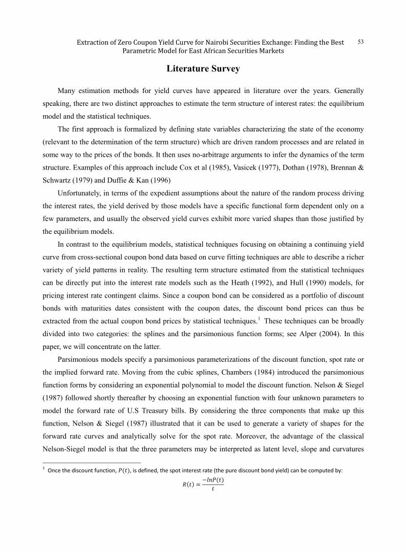
national developments projects, the government issues bonds to investors; this market has traded more and

more volume of these securities in both the primary and secondary markets as the years progress. In 2005,

the trading volume of bonds in the secondary market was Kshs. 246.57 billions, as compared to Kshs.

4.172 trillion in 2012, showing that the Kenyan bond market has truly expanded. Figure 1 shows the

movement of the value of Treasury bonds traded.

Figure 1: Movement of bond’ value (in billions Kshs) traded from 2005 - 2012

Prior to 2000, only treasury bills were available at primary market and virtually no bond market

existed. The issuance of securities was not auction based and there was no market development initiatives.

From 2001, the composition of debt portfolio changed to 76:24 the ratio indicating Treasury bills to bonds.

The average maturity of debt was at 8 months. Then bonds were introduced with the key objective of

lengthening maturity of securities and minimizing refinancing risk. Auction based issuance was adopted to

promote price discovery and development of a yield curve. In addition to this, the Market Leaders Forum

(MLF) was formed so as to support development of the bond market in Kenya.

This led to increased trading in bonds after 2013, the composition of debt portfolio reversed to 26:74,

T-bills to bonds. Average maturity of all securities moved to about 7 years while bonds maturity alone was

5 years. The longest bond in the market is 30-year, issued in 2011. A 20-year was first issued in 2008,

which was followed by a 25-year in 2010. Multi price auction method was introduced which increased

bond market activity, thus providing initial pricing for trading.

According to 2013 CBK report, the CBK plans to start what it dubs as ‘Benchmark Bonds

Programme’. One of the objectives of the programme is to eliminate bond fragmentation at the secondary

market and development of a firm reliable yield curve. This paper aims to be one of the tools the CBK will

use in meeting this objective, by suggesting the best parametric model that should be used in pricing of the

Kenyan bonds.

246.57

1,513.992,469.73

1,198.37

4,095.225,028.54

3,840.89 4,172.21

0.00

1,000.00

2,000.00

3,000.00

4,000.00

5,000.00

6,000.00

2005 2006 2007 2008 2009 2010 2011 2012VA

LUES

IN B

ILLI

ON

S KS

HS.

The value of bonds traded in Kenya


56

Empirical Methodology

4.1 Model Selection

The basis for judging model performance is linked to the expectations from the model. Our

expectation is that the model will be robust in producing stable spot interest rate curves which are efficient

and smooth.

The yield curve can be modelled based on the interest rate function, which could be the forward rate,

discount factor, or zero coupon rates. Given the lack of interest rate derivative markets in Kenya from

which forward rates can be obtained, the general equilibrium models of Vasicek (1977), Cox et al (1985)

and Brennan (1979) are difficult to implement. Hence we do not consider this class of models in

constructing the yield curve. Using the discount factor and/or the zero coupon rates, various models can be

used to construct a yield curve, example the Nelson and Siegel family of models.

4.1.1 The Nelson-Siegel Class of Models

This section will discuss Nelson-Siegel model and its development. Those models are used to

describe the yield curve. Nelson-Siegel model (NS) was first developed by Charles Nelson and Andrew

Siegel from the University of Washington in 1987. This modelling is based on various terms to maturity

that describe yield curve, such as flat, hump, and S- shapes; Nelson & Siegel (1987). This model is

formulated as:

𝑓𝑓𝑚𝑚 (𝑚𝑚;𝑩𝑩, 𝜏𝜏) = 𝛽𝛽0 + 𝛽𝛽1 exp(−𝑚𝑚𝜏𝜏1

) + 𝛽𝛽2𝑚𝑚𝜏𝜏1

exp �− 𝑚𝑚𝜏𝜏1� (1)

Where 𝑓𝑓𝑚𝑚 is the forward rate of government bond in 𝑖𝑖,𝑤𝑤ℎ𝑒𝑒𝑒𝑒𝑒𝑒 𝑖𝑖 = 1, … ,𝑙𝑙; 𝑙𝑙 is number of bonds,

𝑚𝑚 is time to maturity. 𝝉𝝉 = (𝜏𝜏1, 𝜏𝜏2)𝜏𝜏 is also a parameter of maturity, but reflects the times at which the

humps appear in the curve.

�̇�𝜷 is a linear parameter vector. i.e. �̇�𝜷 = (𝛽𝛽0,𝛽𝛽1,𝛽𝛽2,𝛽𝛽3)𝜏𝜏

𝛽𝛽0 is a constant value of forward rate function, it is always constant if maturity period is close to

zero, 𝛽𝛽1determines the initial value of the curve (short term) in various terms of abbreviations, the curve

will be negatively skewed if parameter is positive and vice versa. 𝛽𝛽2 determines magnitude and direction

of the hump curve; if 𝛽𝛽2 is positive then hump will occur 𝜏𝜏1, if 𝛽𝛽2 is negative then U shape will occur

on 𝜏𝜏1, and 𝛽𝛽3 determines magnitude an direction of the second hump, 𝜏𝜏1 is first hump special position

or shape of U curve, 𝜏𝜏2 is second hump position or shape of the U curve. The model that has two humps

is the one introduced by Svensson (1992), (SV Model) which is of the following form:

𝑓𝑓𝑖𝑖�M;𝜷𝜷,̈ �̇�𝜏� = 𝛽𝛽0 + 𝛽𝛽1𝑒𝑒𝑒𝑒𝑒𝑒 �−𝑚𝑚𝜏𝜏1� + 𝛽𝛽2 �

𝑚𝑚𝜏𝜏1

exp �− 𝑚𝑚𝜏𝜏1� � + 𝛽𝛽3 �

𝑚𝑚𝜏𝜏2

exp(−𝑚𝑚𝜏𝜏2

)� (2)


57

The parameters withhold the previous definition indicated above. Rezende (2011) added a third hump

to the SV model to obtain six-factor model (model RF) as follows:

𝑓𝑓𝑖𝑖�M;𝜷𝜷,̈ �̇�𝜏� =

𝛽𝛽0 + 𝛽𝛽1𝑒𝑒𝑒𝑒𝑒𝑒 �−𝑚𝑚𝜏𝜏1� + 𝛽𝛽2 �

𝑚𝑚𝜏𝜏1

exp �− 𝑚𝑚𝜏𝜏1� � + 𝛽𝛽3 �

𝑚𝑚𝜏𝜏2

exp(−𝑚𝑚𝜏𝜏2

)� + 𝛽𝛽4 �𝑚𝑚𝜏𝜏3

exp �− 𝑚𝑚𝜏𝜏3�� (3)

Where 𝑓𝑓𝑖𝑖�Γ;𝜷𝜷,̈ �̇�𝜏� is the forward rate function, 𝑚𝑚 is the time to maturity, (𝛽𝛽0,𝛽𝛽1,𝛽𝛽2,𝛽𝛽3,𝛽𝛽4, )𝜏𝜏 , �̇�𝝉 =

(𝜏𝜏1, 𝜏𝜏2, 𝜏𝜏3)𝑇𝑇, and 𝑖𝑖 = 1, … . , 𝑙𝑙

4.1.2 The Nelson-Siegel (1987) Model

The Nelson-Siegel model sets the instantaneous forward rate at maturity 𝑚𝑚 given by the solution to

a second order differential equation with unequal roots as follows:

𝑓𝑓(𝑚𝑚) = 𝛽𝛽0 + 𝛽𝛽1 𝑒𝑒𝑒𝑒𝑒𝑒 �−𝑚𝑚𝜏𝜏1�+ 𝛽𝛽2 𝑚𝑚

𝜏𝜏1𝑒𝑒𝑒𝑒𝑒𝑒 �−𝑚𝑚

𝜏𝜏2� (4)

Where 𝑚𝑚 > 0. The model consists of four parameters: 𝛽𝛽0,𝛽𝛽1,𝛽𝛽2 and 𝜏𝜏𝑠𝑠 𝑚𝑚 is the time to maturity

of a given bond. Equation (4) consists of three parts: A constant, an exponential decay functional and

Laguerre function. 𝛽𝛽0 is independent of 𝑚𝑚 and as much, 𝛽𝛽0 is often interpreted as the level of long

term interest rates. The exponential decay function approaches zero as 𝑚𝑚 tends to infinity and 𝛽𝛽1 as 𝑚𝑚

tends to zero. The effect of 𝛽𝛽1 is thus only felt at the short end of the curve. The Laguerre function on the

other hand approaches zero as 𝑚𝑚 tends to infinity, and as 𝑚𝑚 tends to zero. The effect of 𝛽𝛽2 is thus only

felt in the middle section of the curve, which implies that 𝛽𝛽2 adds a hump to the yield curve. The spot

rate functions under the model of Nelson and Siegel (1987) is as follows:

𝑒𝑒(𝑚𝑚) = 𝛽𝛽0 + 𝛽𝛽1 �𝜏𝜏1𝑚𝑚� �1 − 𝑒𝑒𝑒𝑒𝑒𝑒 �−𝑚𝑚

𝜏𝜏1�� + 𝛽𝛽2 �

𝜏𝜏2𝑚𝑚� �1 − 𝑒𝑒𝑒𝑒𝑒𝑒 �− 𝑚𝑚

𝜏𝜏2�� − 𝛽𝛽2𝑒𝑒𝑒𝑒𝑒𝑒 �−

𝑚𝑚𝜏𝜏2�

𝑒𝑒(𝑚𝑚) = 𝛽𝛽0 + 𝛽𝛽1 �𝜏𝜏1𝑚𝑚� �1 − 𝑒𝑒𝑒𝑒𝑒𝑒 �−𝑚𝑚

𝜏𝜏1�� + 𝛽𝛽2 �

𝜏𝜏2𝑚𝑚� �1 − 𝑒𝑒𝑒𝑒𝑒𝑒 �− 𝑚𝑚

𝜏𝜏2� �𝑚𝑚

𝜏𝜏2+ 1�� (5)

From equations (4) and (5) it follows that both the spot and forward rate function reduce to 𝛽𝛽0 + 𝛽𝛽1

as 𝑚𝑚 → 0 . Furthermore, we have lim𝑚𝑚→∞ 𝑒𝑒(𝑚𝑚) = lim𝑚𝑚→∞ 𝑓𝑓(𝑚𝑚) = 𝛽𝛽0 . Thus, in the absence of

arbitrage, we must have that 𝛽𝛽0 > 0 and 𝛽𝛽0 + 𝛽𝛽1 > 0

Suppose we observe 𝑙𝑙 zero coupon bonds, expiring at times 𝑚𝑚1,𝑚𝑚2, … ,𝑚𝑚𝑙𝑙 . Let 𝑒𝑒1,𝑒𝑒2, … ,𝑒𝑒𝑙𝑙

denote the prices of these bonds. Note that 𝑒𝑒𝑖𝑖 will imply the spot rate of interest corresponding to time

𝑚𝑚𝑖𝑖 for 𝑖𝑖 = 1, 2, … ,𝑙𝑙. Let 𝑒𝑒1, 𝑒𝑒2, … , 𝑒𝑒𝑙𝑙 denote these spot rates. If we assume that the values of 𝜏𝜏𝑠𝑠 are

known, then the Nelson and Siegel (1987) model reduces to a linear model, which can be solved using

linear regression.

Define:


58

X =

⎝

⎜⎜⎛

1 𝜏𝜏1(1−𝑒𝑒−𝑚𝑚1 𝜏𝜏1⁄ )𝑚𝑚1

𝜏𝜏1(1−𝑒𝑒−𝑚𝑚1 𝜏𝜏1⁄ )𝑚𝑚1

−𝑒𝑒−𝑚𝑚1 𝜏𝜏1⁄

1𝜏𝜏2(1−𝑒𝑒−𝑚𝑚2 𝜏𝜏2⁄ )𝑚𝑚2

𝜏𝜏2(1−𝑒𝑒−𝑚𝑚2 𝜏𝜏2⁄ )𝑚𝑚2

−𝑒𝑒−𝑚𝑚2 𝜏𝜏2⁄

. .. .. .

1𝜏𝜏𝑙𝑙 (1−𝑒𝑒−𝑚𝑚𝑙𝑙 𝜏𝜏𝑙𝑙⁄ )𝑚𝑚𝑙𝑙

𝜏𝜏𝑙𝑙 (1−𝑒𝑒−𝑚𝑚𝑙𝑙 𝜏𝜏𝑙𝑙⁄ )𝑚𝑚𝑙𝑙

−𝑒𝑒−𝑡𝑡𝑙𝑙 𝜏𝜏𝑙𝑙⁄

⎠

⎟⎟⎞

Y = �𝑒𝑒1𝑒𝑒2...𝑒𝑒𝑙𝑙

� B = �𝛽𝛽0𝛽𝛽1𝛽𝛽 2

� (6)

We would like to obtain a vector B satisfying XB = Y + ϵ. By using ordinary least squares (OLS)

estimation, we can solve B as follows:

B = (X ′X)−1X′Y (7)

Nelson and Siegel (1987) suggested the following procedure for calibrating their model:

1. Identify a set of possible values for 𝜏𝜏𝑠𝑠

2. For each of these 𝜏𝜏𝑠𝑠 estimate B

3. For each of these 𝜏𝜏𝑠𝑠 and their corresponding B’s, estimate

𝑅𝑅2 = 1 − ∑ (𝑒𝑒𝑖𝑖−𝑒𝑒̂𝑖𝑖)𝑙𝑙𝑖𝑖=1

∑ (𝑒𝑒𝑖𝑖−𝑒𝑒𝑖𝑖)𝑙𝑙𝑖𝑖=1

(8)

4. The optimal 𝜆𝜆 and 𝛽𝛽 are those associated with the highest value of 𝑅𝑅2.

The above method of calibration is known as the grid-search method. Alternatively, non-linear

optimization techniques can be used to solve all four parameters simultaneously. However, such networks

are very sensitive to starting values, implying a high probability of obtaining local optima. The estimated

parameters obtained by using the grid search method behave erratically over time, and have large

variances. The problems resulting from multi-colinearity depend on the time to maturity of the securities

used to calibrate the model. Diebold (2006), attempted to address the multi-colinearity problem by fixing

the value of 𝜏𝜏𝑠𝑠 over time, which in some instances might not produce accurate results.

Due to the local-minima problem which makes model estimation difficult in the Nelson-Siegel model

and the inadequacy of the calibration methods used so far, we propose NLS estimation with L-BFGS-B

method optimization approach. This optimization method is an extension of the limited memory BFGS

method (LM-BFGS or L-BFGS) which uses simple boundaries model, according to Zhu (1994).

Using L-BGFS-B algorithm, we can estimate the above five parameters: 𝜑𝜑 ≡ {𝛽𝛽0,𝛽𝛽1,𝛽𝛽2, 𝜏𝜏1, 𝜏𝜏2},

embedded in the Nelson–Siegel (1987) model, and hence calculate the price of the bond using the

following nonlinear constrained optimization estimation procedure based the Gauss-Newton numerical

method:

𝑃𝑃𝑖𝑖 = ∑ 𝐶𝐶𝐶𝐶𝑖𝑖𝑚𝑚�1+𝛽𝛽0+𝛽𝛽1�

𝜏𝜏1𝑚𝑚 ��1−𝑒𝑒𝑒𝑒𝑒𝑒 �

−𝑚𝑚𝜏𝜏1��+𝛽𝛽2�


𝑚𝑚𝜏𝜏2��𝑚𝑚𝜏𝜏2

+1��𝑚𝑚 +𝑇𝑇

𝑚𝑚=1 𝜀𝜀𝑖𝑖 (9)

where 𝑃𝑃𝑖𝑖 is the price of bond 𝑖𝑖


59

4.1.3 The Svensson (1992) Model

To increase the flexibility and improve the fitting performance, Svensson (1992) extends Nelson and

Siegel’s (1987) instantaneous forward rate function by adding a fourth term, a second hump (or trough)

𝛽𝛽3 𝑚𝑚𝜏𝜏2𝑒𝑒𝑒𝑒𝑒𝑒 �− 𝑚𝑚

𝜏𝜏2�, with two additional parameters 𝛽𝛽3 and 𝜏𝜏2. The forward rate function is then set as:

𝑓𝑓(𝑚𝑚) = 𝛽𝛽0 + 𝛽𝛽1 𝑒𝑒𝑒𝑒𝑒𝑒 �−𝑚𝑚𝜏𝜏1�+ 𝛽𝛽2 �

𝑚𝑚𝜏𝜏1� 𝑒𝑒𝑒𝑒𝑒𝑒 �−𝑚𝑚

𝜏𝜏1� + 𝛽𝛽3 �


𝜏𝜏2� (10)

Where the unknown parameters 𝛽𝛽0,𝛽𝛽1,𝛽𝛽2 and 𝜏𝜏2 have the same economic interpretation as the

Nelson Siegel model and the two additional parameters 𝛽𝛽3 and 𝜏𝜏2 denote the same meaning as 𝛽𝛽2 and

𝜏𝜏1. The spot rate, derived by integrating the forward rate, is given by:

𝑅𝑅(𝑚𝑚) = 𝛽𝛽0 + 𝛽𝛽1 �𝜏𝜏1

𝑚𝑚��1 − 𝑒𝑒𝑒𝑒𝑒𝑒 �

−𝑚𝑚𝜏𝜏1

��+ 𝛽𝛽2 �𝜏𝜏1



��𝑚𝑚𝜏𝜏2

+ 1�� +

𝛽𝛽3 �𝜏𝜏2𝑚𝑚� �1− 𝑒𝑒𝑒𝑒𝑒𝑒 �−𝑚𝑚


𝜏𝜏2+ 1�� (11)

Similarly, using L-BGFS-B algorithm, we can estimate the parameters and calculate the price using

the following equation:

𝑃𝑃𝑖𝑖 = ∑ 𝐶𝐶𝐶𝐶𝑖𝑖𝑚𝑚�1+𝛽𝛽0+𝛽𝛽1�

𝜏𝜏1𝑚𝑚 ��1−exp �−𝑚𝑚𝜏𝜏1

��+𝛽𝛽2�𝜏𝜏1𝑚𝑚 ��1−exp �−𝑚𝑚𝜏𝜏1

��𝑚𝑚𝜏𝜏1+1��+𝛽𝛽�𝜏𝜏2

𝑚𝑚 ��1−exp �−𝑚𝑚𝜏𝜏2��𝑚𝑚𝜏𝜏2

+1��𝑚𝑚 +𝑇𝑇

𝑚𝑚=1 𝜀𝜀𝑖𝑖 (12)

4.1.4 The Rezende-Ferreira (2011)Model

Rezende Ferreira (2011) decided to increase the accuracy of the Svensson (1992) by adding a fifth

term, a third hump (or trough) 𝛽𝛽4 𝑚𝑚𝜏𝜏3𝑒𝑒𝑒𝑒𝑒𝑒 �− 𝑚𝑚

𝜏𝜏3�, with two additional parameters 𝛽𝛽4 and 𝜏𝜏3. The forward

rate function is then set as:

𝑓𝑓(𝑚𝑚) = 𝛽𝛽0 + 𝛽𝛽1 𝑒𝑒𝑒𝑒𝑒𝑒 �−𝑚𝑚𝜏𝜏1� + 𝛽𝛽2 �


𝜏𝜏1�+ 𝛽𝛽3 �


𝜏𝜏2� + 𝛽𝛽4 �


𝜏𝜏3� (13)

Where the unknown parameters 𝛽𝛽0,𝛽𝛽1,𝛽𝛽2 and 𝜏𝜏2 have the same economic interpretation as the

Nelson Siegel model and the two additional parameters 𝛽𝛽3 and 𝜏𝜏2 denote the same meaning as 𝛽𝛽2 and

𝜏𝜏1. The spot rate, derived by integrating the forward rate, is given by:

𝑅𝑅(𝑚𝑚) = 𝛽𝛽0 + 𝛽𝛽1 �𝜏𝜏1



��+ 𝛽𝛽2 �𝜏𝜏1



��𝑚𝑚𝜏𝜏2

+ 1�� +

𝛽𝛽3 �𝜏𝜏2𝑚𝑚� �1− 𝑒𝑒𝑒𝑒𝑒𝑒 �−𝑚𝑚


𝜏𝜏2+ 1�� + 𝛽𝛽3 �

𝜏𝜏3𝑚𝑚� �1 − 𝑒𝑒𝑒𝑒𝑒𝑒 �−𝑚𝑚


𝜏𝜏3+ 1�� (14)

Similarly, using L-BGFS-B algorithm, we can estimate the parameters and calculate the price using

the following equation:


60

𝑃𝑃𝑖𝑖 =

∑ 𝐶𝐶𝐶𝐶𝑖𝑖𝑚𝑚�1+𝛽𝛽0+𝛽𝛽1�


−𝑚𝑚𝜏𝜏1��+𝛽𝛽2�


−𝑚𝑚𝜏𝜏1��𝑚𝑚𝜏𝜏2

+1��+𝛽𝛽3�𝜏𝜏2𝑚𝑚 � �1−𝑒𝑒𝑒𝑒𝑒𝑒 �−𝑚𝑚𝜏𝜏2

��𝑚𝑚𝜏𝜏2+1��+𝛽𝛽3�

𝜏𝜏3𝑚𝑚 � �1−𝑒𝑒𝑒𝑒𝑒𝑒 �−𝑚𝑚𝜏𝜏3

��𝑚𝑚𝜏𝜏3+1��

𝑚𝑚 +𝑇𝑇𝑚𝑚=1 𝜀𝜀𝑖𝑖

(15)

4.2 Liquidity-Weighted Function

In yield curve construction, errors are caused by two reasons: (a) curve fitting mistakes and (b)

presence of liquidity premium. The errors due to curve fitting arise from the calculations and can be

avoided. But the error due to the presence of liquidity premium is reflective of market conditions and one

cannot ignore them. Since the reliability of the term structure estimation heavily depends on the precision

of the market prices according to Subramanian (2001), liquid and illiquid securities are a heterogeneous

class and including them both in the term structure estimation process poses problems. Illiquid bonds are

traded at a premium to compensate for their undesirable attribute in terms of a low price. Assigning equal

weights to both types of errors will give undue weight to the kind of error that creeps in due to curve

fitting.

Subramanian (2001) suggests a liquidity weighted objective function, which hypothesizes that a

weighted error function (with weights based on liquidity) would lead to better estimation that equal

weights to the squared errors of all securities. We therefore model the liquidity using a function with two

factors: the volume of trade in a security and the number of trades in that security.

The weight of the 𝑖𝑖𝑡𝑡ℎ security 𝑊𝑊𝑖𝑖 is given by:

𝑊𝑊𝑖𝑖 =��1−𝑒𝑒

�−𝑣𝑣𝑖𝑖

𝑣𝑣𝑚𝑚𝑚𝑚𝑒𝑒��+�1−𝑒𝑒

�− 𝑙𝑙𝑖𝑖

𝑙𝑙𝑚𝑚𝑚𝑚𝑒𝑒��

∑ 𝑊𝑊𝑖𝑖𝑖𝑖= �1 − 𝑒𝑒�−

𝑣𝑣𝑖𝑖𝑣𝑣𝑚𝑚𝑚𝑚𝑒𝑒

�� + �1 − 𝑒𝑒�− 𝑙𝑙𝑖𝑖𝑙𝑙𝑚𝑚𝑚𝑚𝑒𝑒

�� (16)

𝑊𝑊𝑖𝑖 =�tanh �− 𝑣𝑣𝑖𝑖

𝑣𝑣𝑚𝑚𝑚𝑚𝑒𝑒�+tanh �− 𝑙𝑙𝑖𝑖

𝑙𝑙𝑚𝑚𝑚𝑚𝑒𝑒��

∑ 𝑊𝑊𝑖𝑖𝑖𝑖= tanh �− 𝑣𝑣𝑖𝑖

𝑣𝑣𝑚𝑚𝑚𝑚𝑒𝑒� + tanh �− 𝑙𝑙𝑖𝑖

𝑙𝑙𝑚𝑚𝑚𝑚𝑒𝑒� (17)

Where 𝑣𝑣𝑖𝑖 and 𝑙𝑙𝑖𝑖 are the volume of trade and the number of trades in the 𝑖𝑖𝑡𝑡ℎ security respectively,

while 𝑣𝑣𝑚𝑚𝑚𝑚𝑒𝑒 and 𝑙𝑙𝑚𝑚𝑚𝑚𝑒𝑒 are the maximum number of trades among all the securities traded for the day

respectively.

As given in the equations (16) and (17) above, it ensures that the weights of the relative liquid

securities would not be significantly different from each other. For the illiquid securities, however the

weights would fall quickly as liquidity decreased.

The final error-minimizing function, which should equal to zero, is given by:

𝑀𝑀𝑖𝑖𝑙𝑙∑ 𝑤𝑤𝑖𝑖(𝑃𝑃𝑖𝑖 − 𝐵𝐵𝑖𝑖)2𝑙𝑙𝑖𝑖=1 = 𝑀𝑀𝑖𝑖𝑙𝑙∑ 𝑤𝑤𝑖𝑖𝜀𝜀𝑖𝑖2𝑙𝑙

𝑖𝑖=1 = 0 (18)


61

4.3 Liquidity-Weighted Function

In academic literature, there are two distinct approaches used to indicate the term structure fitting

performance. One is the flexibility of the curve (accuracy), and the other focuses on smoothness of the

yield curve. Although there are numerical methods proposed to estimate the term structure, any method

developed has to grapple with deciding the extent of the above trade-off. Hence it becomes a crucial issue

to investigate how to reach a compromise between the flexibility and smoothness.

Three simple summary statistics which can be calculated for the flexibility of the estimated yield

curve are the coefficient of determination, root mean squared percentage error, and root mean squared

error . These are calculated as:

4.3.1 The Coefficient of Determination (R2)

𝑅𝑅2 = 1 − ∑ (𝑃𝑃𝑖𝑖−𝐵𝐵𝑖𝑖�)2 (𝑙𝑙−𝑘𝑘)⁄𝑙𝑙𝑖𝑖=1

∑ (𝑃𝑃𝑖𝑖−𝑃𝑃𝑖𝑖� )2 (𝑙𝑙−1)⁄𝑙𝑙𝑖𝑖=1

(19)

where 𝑃𝑃� is the mean average price of all observed bonds, 𝐵𝐵𝑖𝑖� is the model price of a bond 𝑖𝑖, 𝑙𝑙 the

number of bonds traded and 𝑘𝑘 is the number of parameters needed to be estimated.

Roughly speaking, with the same analysis in regression, we associate a high value of 𝑅𝑅2 with a good

fit of the term structure and associate a low 𝑅𝑅2 with a poor fit.

4.3.2 Root Mean Squared Error (RMSE)

Denoted as the RMSE, a low value for this measure is assumed to indicate that the model is flexible,

on average, and is able to fit the yield curve.

𝑅𝑅𝑀𝑀𝑅𝑅𝑅𝑅 = �1𝑙𝑙∑ �𝑃𝑃𝑖𝑖 − 𝐵𝐵𝑖𝑖� �

2𝑙𝑙𝑖𝑖=1 (20)

4.3.3 Root Mean Squared Percentage Error (RMSPE)

Denoted as the RMSPE, a low value for this measure is also assumed to indicate that the model is

flexible, on average, and is able to fit the yield curve.

𝑅𝑅𝑀𝑀𝑅𝑅𝑃𝑃𝑅𝑅 = �1𝑙𝑙∑ �𝑃𝑃𝑖𝑖−𝐵𝐵𝑖𝑖

�𝑃𝑃𝑖𝑖

�2

× 100%𝑙𝑙𝑖𝑖=1 (21)

4.3.4 Testing for Smoothness

To test the smoothness of the estimated yield curve, we use a modified statistic suggested by Adams

and Deventer (1994) to reach the maximum smoothness for forward rate curve, and denote the smoothness

(𝑍𝑍) for the estimated yield curve as:

𝑍𝑍 = ∑ ��𝑓𝑓(𝑡𝑡) − 𝑓𝑓(𝑡𝑡 − 12)� − �𝑓𝑓 �𝑡𝑡 − 1

2� − 𝑓𝑓(𝑡𝑡 − 1)��

2𝑙𝑙𝑡𝑡=1.5 × 1

2= 0 (22)


62

Ideally, the value should equal to zero. The model with the least 𝑍𝑍 value is deemed to be the best.

Empirical Results

5.1 Data

In Kenya, nearly all bond transactions take place on the OTC market. The data used in this study was

supplied by the Central Bank of Kenya. The sample period contains 417 weekly data from January 2005 to

December 2012. Weekly prices (every Friday) for 108 Kenyan Government Bonds (KGBs) with original

maturity dates ranged from 2 to 30 years are obtained.

Our expectation is that the model will be robust in producing stable spot interest rate curves which

are efficient and smooth.

5.2 Parameter Estimation

5.2.1 Nelson-Siegel (1987) Model

Table 1 lists the summary statistics of estimated parameters for the Nelson-Siegel (1987) model. It is

seen that all estimated values for 𝛽𝛽1� and 𝛽𝛽2� are negative, which indicates that the yield curves generated

by this model are all positively and upward sloping without a visible hump.

Table 1: Results for estimated parameters for Nelson-Siegel (1987) Model

Year Parameters

�̂�𝛽0 �̂�𝛽1 �̂�𝛽2 𝜏𝜏1�

2005 0.0587 -0.0115 -0.0040 4.6089

2006 0.0463 -0.0090 -0.0127 3.2148

2007 0.0454 -0.0133 -0.0388 1.8327

2008 0.0356 -0.0183 -0.0425 2.1674

2009 0.0358 -0.0164 -0.0493 1.0232

2010 0.0225 -0.0085 -0.0819 0.6237

2011 0.0225 -0.0085 -0.0819 0.6237

2012 0.0241 -0.091 -0.0213 1.0595

5.2.2 Svensson (1992) model

Table 2 reports the summary statistics of estimated parameters for the Svensson (1992) model. We

find that, in the particular years 2007, 2010, 2011 and 2012, the estimated 𝛽𝛽1� is negative while the


63

estimated 𝛽𝛽2� is positive, showing the yield curves would have a positively upward sloping combined

with a slightly humped shape.

Table 2: Results for estimated parameters for Svensson (1992) Model

Year Parameters

�̂�𝛽0 �̂�𝛽1 �̂�𝛽2 �̂�𝜏1 �̂�𝜏2

2005 0.0590 -0.0138 -0.0010 2.1459 3.3983

2006 0.0473 -0.0121 -0.0068 2.5956 3.8261

2007 0.0425 -0.0182 0.0020 3.3964 5.4206

2008 0.0370 -0.0189 -0.0333 2.5649 8.1488

2009 0.0354 -0.0181 -0.0309 2.8238 7.6419

2010 0.0248 -0.0129 0.0025 8.0086 15.4666

2011 0.0248 -0.0129 0.0025 8.0086 15.4666

2012 0.0250 -0.0114 0.0072 3.3570 4.1933

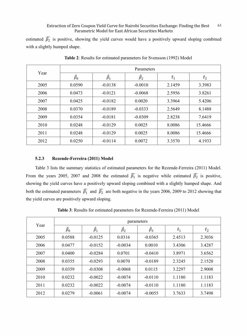
5.2.3 Rezende-Ferreira (2011) Model

Table 3 lists the summary statistics of estimated parameters for the Rezende-Ferreira (2011) Model.

From the years 2005, 2007 and 2008 the estimated 𝛽𝛽1� is negative while estimated 𝛽𝛽2� is positive,

showing the yield curves have a positively upward sloping combined with a slightly humped shape. And

both the estimated parameters 𝛽𝛽1� and 𝛽𝛽2� are both negative in the years 2006, 2009 to 2012 showing that

the yield curves are positively upward sloping.

Table 3: Results for estimated parameters for Rezende-Ferreira (2011) Model

Year parameters

�̂�𝛽0 �̂�𝛽1 �̂�𝛽2 �̂�𝛽3 �̂�𝜏1 �̂�𝜏2

2005 0.0588 -0.0125 0.0316 -0.0365 2.4513 2.3036

2006 0.0477 -0.0152 -0.0034 0.0010 3.4306 3.4287

2007 0.0400 -0.0284 0.0701 -0.0410 3.8971 3.6562

2008 0.0355 -0.0293 0.0070 -0.0189 2.3245 2.1520

2009 0.0359 -0.0308 -0.0068 0.0115 3.2297 2.9008

2010 0.0232 -0.0022 -0.0074 -0.0110 1.1180 1.1183

2011 0.0232 -0.0022 -0.0074 -0.0110 1.1180 1.1183

2012 0.0279 -0.0061 -0.0074 -0.0055 3.7633 3.7498


64

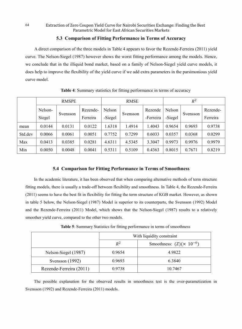
5.3 Comparison of Fitting Performance in Terms of Accuracy

A direct comparison of the three models in Table 4 appears to favor the Rezende-Ferreira (2011) yield

curve. The Nelson-Siegel (1987) however shows the worst fitting performance among the models. Hence,

we conclude that in the illiquid bond market, based on a family of Nelson-Siegel yield curve models, it

does help to improve the flexibility of the yield curve if we add extra parameters in the parsimonious yield

curve model.

Table 4: Summary statistics for fitting performance in terms of accuracy

RMSPE RMSE 𝑅𝑅2

Nelson-

Siegel Svensson

Rezende-

Ferreira

Nelson

-Siegel Svensson

Rezende

-Ferreira

Nelson

-Siegel Svensson

Rezende-

Ferreira

mean 0.0144 0.0131 0.0122 1.6318 1.4914 1.4043 0.9654 0.9693 0.9738

Std.dev 0.0066 0.0061 0.0051 0.7752 0.7299 0.6033 0.0357 0.0368 0.0299

Max 0.0413 0.0385 0.0281 4.6311 4.5345 3.3047 0.9973 0.9976 0.9979

Min 0.0050 0.0048 0.0041 0.5311 0.5109 0.4363 0.8015 0.7671 0.8219

5.4 Comparison for Fitting Performance in Terms of Smoothness

In the academic literature, it has been observed that when comparing alternative methods of term structure

fitting models, there is usually a trade-off between flexibility and smoothness. In Table 4, the Rezende-Ferreira

(2011) seems to have the best fit in flexibility for fitting the term structure of KGB market. However, as shown

in table 5 below, the Nelson-Siegel (1987) Model is superior to its counterparts, the Svensson (1992) Model

and the Rezende-Ferreira (2011) Model, which shows that the Nelson-Siegel (1987) results to a relatively

smoother yield curve, compared to the other two models.

Table 5: Summary Statistics for fitting performance in terms of smoothness

With liquidity constraint

𝑅𝑅2 Smoothness: (𝑍𝑍)(× 10−6)

Nelson-Siegel (1987) 0.9654 4.9822

Svensson (1992) 0.9693 6.3840

Rezende-Ferreira (2011) 0.9738 10.7467

The possible explanation for the observed results in smoothness test is the over-parametization in

Svensson (1992) and Rezende-Ferreira (2011) models.


65

5.5 Conclusion and Discussion of Results

After investigating the three parametric models of Nelson-Siegel Class, we decided to use on the

Nelson-Siegel (1987) Model. This is because it gave the best performance in terms of smoothness of the

forward curve, which is very importance since it points towards the differentiability of the curve which results

to attainability of spot curves. Another reason we settled on this parametric model is that according to Bank of

International Settlements (2005), which is a technical reports on how central banks around the world calculate

the ZCYC, it reports that central banks around the world do not typically require yield curve models that price

back all the inputs exactly, when determining monetary policy. A curve does not have to have 100% accuracy;

95% and above is deemed as adequate. We see that Nelson-Siegel (1987) Model has 96.54% accuracy level,

which is above the required 95%.

In addition to the tests indicated above, we decided to use two additional test tools to check the adequacy

of the Nelson-Siegel (1987) Model. These tools are: a) the monotonicity of the discount factors curve and b) the

comparison between the observed bonds’ dirty prices and the model’s dirty prices. The following were the

results achieved:

Figure 2: NS discount graph: showing that the discount function is a decreasing function of time

0.82178

0.0%

20.0%

40.0%

60.0%

80.0%

100.0%

120.0%

0 2 4 6 8 10

Price

of

Bonds

Time in years

N&S Discount Factors


66

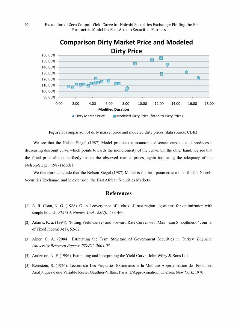
Figure 3: comparison of dirty market price and modeled dirty prices (data source: CBK)

We see that the Nelson-Siegel (1987) Model produces a monotonic discount curve; i.e. it produces a

decreasing discount curve which points towards the monotonicity of the curve. On the other hand, we see that

the fitted price almost perfectly match the observed market prices, again indicating the adequacy of the

Nelson-Siegel (1987) Model.

We therefore conclude that the Nelson-Siegel (1987) Model is the best parametric model for the Nairobi

Securities Exchange, and in extension, the East African Securities Markets.

References

[1]. A. R. Conn, N. G. (1988). Global covergence of a class of trust region algorithms for optimization with simple bounds, SIAM J. Numer. Anal., 25(2):, 433-460.

[2]. Adams, K. a. (1994). "Fitting Yield Curves and Forward Rate Curves with Maximum Smoothness," Journal of Fixed Income,4(1), 52-62.

[3]. Alper, C. A. (2004). Estimating the Term Structure of Government Securities in Turkey. Bogazaci University Research Papers: ISS/EC -2004-03.

[4]. Anderson, N. F. (1996). Estimating and Interpreting the Yield Curve. John Wiley & Sons Ltd.

[5]. Bernstein, S. (1926). Lecons sur Les Properties Extremates et la Meillure Approximation des Fonctions Analytiques d'une Variable Reete, Gauthier-Villars, Paris; L'Approximation, Chelsea, New York, 1970.

90.00%

100.00%

110.00%

120.00%

130.00%

140.00%

150.00%

160.00%

0.00 2.00 4.00 6.00 8.00 10.00 12.00 14.00 16.00 18.00

Modified Duration

Comparison Dirty Market Price and Modeled Dirty Price

Dirty Market Price Modeled Dirty Price (fitted to Dirty Price)


67

[6]. Bliss, R. (1996, November). Testing Term Strucuture Estimation Methods. Federal Reserve Bank of Atlanta, Working Paper 96-12a.

[7]. Bliss, R. (1997). "Testing Term Structures Estimation Methods," Advances in Futures and Options Research,9,197-232.

[8]. Bolder, D. a. (1999). Yield Curve Modelling at the Bank of Canada. Technical Report , 84.

[9]. Brennan, M., & Schwartz, a. E. (1979). A Continous - Time Approach to the Pricing of Bonds. Journal of Banking and Finance, 3 (2), 133-156.

[10]. Broyden., C. (1970). The convergence of a class of double-rank minimization algorithms. II.The New algorithm. . J. Inst. Math. Appl.,6, 222-231.

[11]. Chambers, D. .. (1984). A New Approach to Estimation of the Term Structure of Interest Rate. Journal of Finanacial and Qualitative Analysis, 19 (3), 233-252.

[12]. Choundry, M. D. (2001). Capital Markets Instruments Analysis and Valuation . FT Prentice Hall .

[13]. Christofi, A. (1998). Estimation o the Nelson -Siegel Parimonious Modelling of Yield Curves Using An Exponential GARCH Process. Managerial Finance , 24 (9-10), 1-19.

[14]. Ciyou Zhu, R. B.-B.-B. (2011). www.ece.northwestern.edu. Retrieved from

http://www.ece.northwestern.edu/nocedal/lbfgsb.html,.

[15]. Ciyou Zhu, R. H. (1997). Algorithm 778:L-BFGS-B:Fortran: Fortran subroutines for large-scale bound-contrained optimization . ACM Trans, Math,. Software, 23(4), 550-560.

[16]. Cox, J. a. (1985). "A Theory of Term Structure of Interest Rates," Econometrica,53(2),385-407.

[17]. Deacon, M. a. (1994). Estimating the Term Structure of Interest Rates. Working Paper No. 24 , Bank of England.

[18]. Deventer, A. a. (1994). Fitting Yield Curves and Forward Rate Curves with Maximum Smoothness. Journal of Fixed Income, 52-62.

[19]. Diebold, F. a. (2006). Forecasting the Term Strucuture of Government Bond Yields. Journal of Econometrics 130 (2), 337-364.

[20]. Dothan, L. (1978). On the Term Strcuture of Interest Rates. Journal of Financial Economies, 6 (1), 59-69.

[21]. Duffie D, a. R. (1996). A Yield Factor Model of Interest Rates. Mathematical Finance, 6 (4), 379-406.

[22]. Ecom, Y. (1998). Subrahmanyam,M.G. and Uno,J. "Coupon effects and the pricing of Japanese Government Bonds: An Emphirical Analysis", Journal of Fixed Income, September,69-86.


68

[23]. Fama, E. a. (1987). The Information in the Long Maturity Foward Rates. Amwerican Economic Review , 77( 4), 680-692.

[24]. Fisher, M. a. (1995). "Fitting the Term structure of Interest Rates with Smoothing Splines," Working paper 95-1, Finance and Economics Discussion Series, Federal Reserve Board.

[25]. Fletcher., R. (1970). A new approach to viable metric algorithms. The computer Journals, 13(3), 317-322.

[26]. Gilli, M. G. (2010). Calibrating the Nelson-Siegel -Svensson Model. Comisef, 031.

[27]. Goldfarb, D. (1970). A family of variable metricmethods derived by variational means. math comp, 24:, 23-26.

[28]. Griva, I. N. (2009). Linear and Nonlinear Optimization. Siam.

[29]. Hartley, H. (1961). The Modified Gauss Newton Method or the Fitting of Non-Linear Regression Functions by Least Squares. Technometrics , 3 (2), 269-280.

[30]. Heath, D. (1992). Bond Pricing and the Term Structure of Interest Rates: A new Methodology for Contigent Claim Valuation. Econometrica , 60 (1), 77-105.

[31]. Hull, J. a. (1990). Pricing Interest Rate Derivatives Securities. Review of Financial Studies, 3 (4), 573-592.

[32]. Ingersoll, J. (1987 ). Theory of Financial Decision Making . Bowman and Littlefield , Chapter 18.

[33]. Jarrow, R. (2004). Estimating the Interest Rate Term Structure of Corporate Debt with a Semi-parametric Penalized Spline Model. Journal of the American Statistical Association, 99 (465), 57-66.

[34]. Jarrow. (1996). Modelling Fixed Incomen Securities and Interest Rate Options, . McGraw-Hill , Chapters 2-3 .

[35]. Jeffrey A., O. L. (2000). Flexible Term Structure Estimation: Which Method is Preferred? In Yale SOM Working Paper No. ICF -00-25. International Center for Finance.

[36]. John C. Cox, J. E. (1985). A Theory of the Term Structure of Interest Rates. Econometrica volume 53,issue 2, 385-408.

[37]. Kelly, C. T. (1999). Iteratrive Methods for Optimization . Siam, Philadephia.

[38]. Krivobokova, T. K. (2006). Estimating the Term Structure of Interest Rates Using Penalized Splines. Statistical Papers, 47, 443-459.

[39]. Lin, B. (2002). Fitting Term Structure of Interest Rates Using B-Splines: the Case of Taiwanese Government Bonds. Applied Financial Economies, 12 (1), 57-75.


69

[40]. Lin, B. a. (1993). Valuing the New Issue Quality Option in Bund Futures. Review of Future Markets 12 (2), 249-388.

[41]. Linton, O. E. (2001). Yield Curve Estimation by Kernel Smoothing Methods. Journal of Econometrics 105 (1), 185-223.

[42]. M., I. (2003). A Comparison of the Yield Curve Estimation TechniquesUsing UK Data. Journal of Banking and Finance 27 (1), 1-26.

[43]. Maria, A. L. (2009). Estimation iof the Term Structure of Interest Rates: The Venezuelan Case. Journal of Future Markets, 23, 1075-105.

[44]. Mastronikola, K. (1991, December). Yield Curve for Gilt Edged Stocks: A New Model. Bank of England Discussion Paper (Techinical Series).

[45]. McCulloch, J. (1975). The Tax Adjusted Yield Curve. Journal of Finance, 811-830.

[46]. McCulloh, J. (1971). "Measuring the Term Structure of Interest Rates," Journal of Business 34, 19-31.

[47]. Modena, M. (2008). An Empirical Analysis of the Curvature Factor of the Term Structure of Interest Rates. MPRA Paper, No. 11597.

[48]. Nelson, C. F. (1987). Parsimonious Modelling of Yield Curves. Journal of Business 60, 473-89.

[49]. Nocedal., J. (1980). Updating quasi-Newton matrices with limited storage. Math Comp., 35(151):, 773-782.

[50]. Overton., A. S. (2013). Nonsmooth optimization via quasi-Newton methods. Math. Program., 141(1-2, Ser. A):, 135-163 .

[51]. Ramsey, J. B. (1969). Tests for Specific Errors in Classical Linear Least-Squares Regression Analysis. Journal of the Royal Stastical Society,31, 350-371.

[52]. Rezende, R. D. (2011). Modelling and Forecasting the Yield Curve by an Extended Nelson and Siegel Class of Models: A Quatile Autoregression Approach. Journal of Forecasting, 32, 111-123.

[53]. Richard, H. B. (1995). A limited memory algorithm for bound constrained optimizaton. SIAM J. Sci. Comput, 16(5), 1190-1208.

[54]. Rosadi, D. (2011). Modelling of Yield Curve and Its Computation by Software Packeges RemdrPlugin. Econometric. Proceeding FMIPA UnDip 2011, 514-523.

[55]. Schaefer, S. (1981). Measuring a Tax-Specific Term Strucuture of Interest Rates in the Market of British Government Securities. The Economic Journal, 415-438.


70

[56]. Shanno, D. (1970). Conditioning of quasi-Newton methods for fucntion minimization. Math Comp., 24, 647-656.

[57]. Shea, G. (1985). Interest Rate Term Structure Estimation with Exponential Splines. The Journal of Finace 40, (1), 319-325.

[58]. Shiller, R. (1990). The Term Structure of Interest Rates . Handbook of Monetary Economics, Chapter 3.

[59]. Steeley, J. (1991). Estimating the Gilt -Edged Term Structure Basis Spline and Confidence. Journal of Business Finance and Accounting, 18 (4), 513-529.

[60]. Subramanian, K. (2001). Term Structure Estimation in Illiquid Markets. The Journal of Fixed Income, 11, 77-86.

[61]. Svensson, L. (1992). Estimating and Interpreting Foward Interest Rates. NBER Working Paper Series 4871.

[62]. Tam, C. a. (2008). Modelling Sovereign Bond Yields Curves of the US, Japan and Germany. International Journal of Finanace and Economics, 13, 82-91.

[63]. Toraldo., J. J. (1989 ). Algorithms for bound constrained quadratic programming problem. Numer. Math., 55(4):, 377- 400.

[64]. Vasiceck, O. (1977). An Equilibruim Characterization of the Term Structure. Journal of Financial Economies,5 (2), 177-188.

[65]. Vasiceck, O. a. (1982). Term Structure Estimation Using Exponential Splines. Journal of Finance, 339-348.

[66]. Waggoner, F. D. (1997). "Spline methods for Extracting Interest Rate curves from Coupon Bond Prices," Working paper 97-10, Federal Reserve Bank of Atlanta.

[67]. Wilmer Henao. (2014). L-BFGS-B-NS, www.github.com. Retrieved from

https://github.com/wilmerhenao/L-BFGS-B-NS,.

[68]. Wright, J. N. (1999). Numerical optimization. Springer series in Operations Research Springer-Vrlag, New York.

[69]. Yeh, S. a. (2003). Term Strucuture Fitting Models and Information Content: An Empirical Examination In Taiwanese Government Bond Market. Review of Pacific Basin Financial Market and Policies, 305-348.

[70]. Zhu, C. B. (1994). L-BFGS-B Fortran Subroutines for Large-Scale Bouynd Constrainjed Optimization, Department of Eelectrical Engineering and Computer Science, Northwestern University.


71

Appendix I: The L-BFGS-B Algorithm

A.1.1. Introduction The problem addressed is to find a local minimizer of the non-smooth minimization problem.

𝑚𝑚𝑖𝑖𝑙𝑙𝑒𝑒𝑥𝑥ℝ𝑙𝑙 𝑓𝑓(𝑒𝑒) (A1)

𝑠𝑠. 𝑡𝑡. 𝑙𝑙𝑖𝑖 ≤ 𝑒𝑒𝑖𝑖 ≤ 𝑢𝑢𝑖𝑖 𝑖𝑖 = 1, … . ,𝑙𝑙.

Where 𝑓𝑓:ℝ𝑙𝑙 → ℝ is continuous but not differentiable anywhere and 𝑙𝑙 is large. 𝑙𝑙𝑖𝑖 and 𝑢𝑢𝑖𝑖 are respectively an upper limit and; lower limit parameters. 𝑓𝑓(𝑒𝑒) is NLS (Non Linear Schrödinger) function of residual functions of Nelson-Siegel model class and 𝑒𝑒 is a parameter of the Nelson-Siegel model class.

The L-BFGS-B algorithm by Richard (1995) is a standard method for solving large instances of

𝑚𝑚𝑖𝑖𝑙𝑙𝑒𝑒𝑥𝑥ℝ𝑙𝑙 𝑓𝑓(𝑒𝑒) when 𝑓𝑓 is a smooth function, typically twice differentiable.

The name BFGS stands for Broyden, Fletcher, and Goldfarb and Shanno, the originators of the BFGS quasi-Newton algorithm for unconstrained optimization discovered and published independently by them in 1970 [Broyden (1970), Fletcher (1970), Goldfarb (1970) and Shanno (1970)]. This method requires storing and updating a matrix which approximates the inverse of the Hessian ∇2𝑓𝑓(𝑒𝑒) and hence requires 𝒪𝒪(𝑙𝑙2) operations per iteration. According to Nocedal (1980), the L-BFGS variant where the L stands for “Limited-Memory” and also for “Large” problems, is based on BFGS but requires only 𝒪𝒪(𝑙𝑙) operations per iteration, and less memory. Instead of storing the 𝑙𝑙 × 𝑙𝑙 Hessian approximations, L-BFGS stores only 𝑚𝑚 vectors of dimesion 𝑙𝑙, where 𝑚𝑚 is a number much smaller than 𝑙𝑙. Finally, the last letter B in L-BFGS stands for bounds, meaning the lower and upper bounds 𝑙𝑙𝑖𝑖 and 𝑢𝑢𝑖𝑖 . The L-BFGS-B algorithm is implemented in a FORTRAN software package, according to Zhu et al (2011). We discuss how to modify the algorithm for non-smooth functions.

A.1.2. BFGS BFGS is standard tool for optimization of smooth functions. It is a line search method. The search

direction is of type𝑑𝑑 = −𝐵𝐵𝑘𝑘∇𝑓𝑓(𝑒𝑒𝑘𝑘) where 𝐵𝐵𝑘𝑘 approximation to the inverse Hessian of 𝑓𝑓.4 This 𝑘𝑘𝑡𝑡ℎ step approximation is calculated via the BFGS formula.

𝐵𝐵𝑘𝑘+1 = �𝐼𝐼 − 𝑠𝑠𝑘𝑘𝑦𝑦𝑘𝑘𝑇𝑇

𝑦𝑦𝑘𝑘𝑇𝑇𝑠𝑠𝑘𝑘�𝐵𝐵𝑘𝑘 �𝐼𝐼 −

𝑦𝑦𝑘𝑘𝑠𝑠𝑘𝑘𝑇𝑇

𝑦𝑦𝑘𝑘𝑇𝑇𝑠𝑠𝑘𝑘� + 𝑠𝑠𝑘𝑘𝑠𝑠𝑘𝑘

𝑇𝑇

𝑦𝑦𝑘𝑘𝑇𝑇𝑠𝑠𝑘𝑘

(A2)

Where 𝑦𝑦𝑘𝑘 = ∇𝑓𝑓(𝑒𝑒𝑘𝑘+1)− ∇𝑓𝑓(𝑒𝑒𝑘𝑘) and 𝑠𝑠𝑘𝑘 = 𝑒𝑒𝑘𝑘+1 − 𝑒𝑒𝑘𝑘 . BFGS exhibits super-linear convergence on generic problems but it requires 𝒪𝒪(𝑙𝑙2) operations per iteration, according to Wright (1999).

In the case of non-smooth functions, BFGS typically succeeds in finding a local minimizer, as indicated by Overton (2013). However, this requires some attention to the line search conditions. This conditions are known as the Armijo and weak Wolfe line search conditions and they are a set of inequalities used for computation of an appropriate step length that reduces the objective function “sufficiently”.

4 When it is exactly the inverse Hessian this method is known as Newton method. Newton’s method has quadratic convergence but requires the explicit calculation of the Hessian at every step.


72

A.1.3. L-BFGS L-BFGS stands for Limited-memory BFGS. This algorithm approximates BFGS using only a limited

amount of computer memory to update an approximation to the inverse of the Hessian of 𝑓𝑓. Instead of storing a dense 𝑙𝑙 × 𝑙𝑙 matrix, L-BFGS keeps a record of the last 𝑚𝑚 is a small number that is chosen in advance. For this reason the first 𝑚𝑚 iterations of BFGS and L-BFGS produce exactly the same search directions if the initial approximation of 𝐵𝐵0 is set to the identity matrix.

Because of this construction, the L-BFGS algorithm is less computationally intensive and requires only 𝒪𝒪(𝑚𝑚𝑙𝑙) operations per iteration. So it is much better suited for problems where the number of dimensions 𝑙𝑙 is large.

A.1.4. L-BFGS-B Finally L-BFGS-B is an extension of L-BFGS. The B stands for the inclusion of Boundaries. L-BFGS-B

requires two extra steps on top of L-BFGS. First, there is a step called gradient projection that reduces the dimensionality of the problem. Depending on the problem, the gradient projection could potentially save a lot of iterations by eliminating those variables that are on their bounds at the optimum reducing the initial dimensionality of the problem and the number of iterations and running time. After this gradient projection comes to second step of subspace minimization. During the subspace minimization phase, an approximate quadratic model of (A1) is solved iteratively in a similar way that the original L-BFGS algorithm is solved. The only difference is that the step length is restricted as much as necessary in order to remain within the lu-box defined by equation (A1).

A.1.5. Gradient Projection The L-BFGS-B algorithm was designed for the case when n is large and 𝑓𝑓 is smooth. Its first step is the

gradient projection similar to the one outlined in Conn (1988) and Toraldo (1989 ), which is used to determine an active set corresponding to those variables that are on either their lower or upper bounds. The active set is defined at point 𝑒𝑒∗ is:

𝒜𝒜(𝑒𝑒∗) = {𝑖𝑖ϵ{1 … .𝑙𝑙}\𝑒𝑒𝑖𝑖∗ = 𝑙𝑙𝑖𝑖 ⋁ 𝑒𝑒𝑖𝑖∗ = 𝑢𝑢𝑖𝑖} (A3) Working with this active set is more efficient in large scale problems. A pure line search algorithm would

have to choose to step length short enough to remain within the box defined by 𝑙𝑙𝑖𝑖 and 𝑢𝑢𝑖𝑖 . So if at the optimum, a large number ℬ of variables are either on the lower or upper bound, as many as ℬ of iterations might be needed. Gradient projection tries to reduce this number of iterations. In the best case, only one iteration is needed instead of 𝓑𝓑.

Gradient projections works on the linear part of the approximation model:

𝑚𝑚𝑘𝑘(𝑒𝑒) = 𝑓𝑓(𝑒𝑒𝑘𝑘) + ∇𝑓𝑓(𝑒𝑒𝑘𝑘)𝑇𝑇(𝑒𝑒 − 𝑒𝑒𝑘𝑘) + (𝑒𝑒−𝑒𝑒𝑘𝑘)𝑇𝑇𝐻𝐻𝑘𝑘(𝑒𝑒−𝑒𝑒𝑘𝑘)2

(A4)

Where 𝐻𝐻𝑘𝑘 is a L-BFGS-B approximation to the Hessian ∇2𝑓𝑓 stored in the implicit way defined by L-BFGS.

In this first stage of the algorithm a piece-wise linear path starts at the current point 𝑒𝑒𝑘𝑘 in the direction−∇𝑓𝑓(𝑒𝑒𝑘𝑘). Whenever this direction encounters one of the constraints the path runs corners in order to remain feasible. The path is nothing but feasible piece-wise projection of the negative gradient direction on the constraint box determined by the values 𝑙𝑙 and 𝑢𝑢. At the end of this stage, the value of 𝑒𝑒 that minimizes


73

𝑚𝑚𝑘𝑘(𝑒𝑒) restricted to this piece-wise gradient path is known as the “Cauchy point” 𝑒𝑒𝑐𝑐 . From this description of the estimation and optimization, following steps can be summarized: Find the residual function (r) of each model.

Find NLS estimation, i.e. 𝑓𝑓(𝑒𝑒𝑖𝑖) = 12Σ𝑖𝑖=1𝑒𝑒 [𝑒𝑒𝑖𝑖]2, of each model.

Find the 𝑒𝑒 × 𝑒𝑒 matrix value for 𝐵𝐵1 = 𝐼𝐼, 𝑒𝑒 is the number of parameters estimated in each model.

Find the initial value of parameter vector with rank 𝑒𝑒 × 1, 𝑒𝑒 is the number of parameters estimated in each model.

Find gradient from step 2 with every parameter in models. e.g. ∇𝑓𝑓(𝑒𝑒𝑖𝑖)𝑖𝑖 Substitute the initial value of the parameter (step 3) to gradient of step 5 with result. e.g.

𝛻𝛻𝑓𝑓(𝑒𝑒1). Find the value of 𝑒𝑒1 Find the value of 𝑓𝑓(𝑒𝑒1) so it will obtain of 𝑑𝑑1 and 𝑠𝑠1.


74

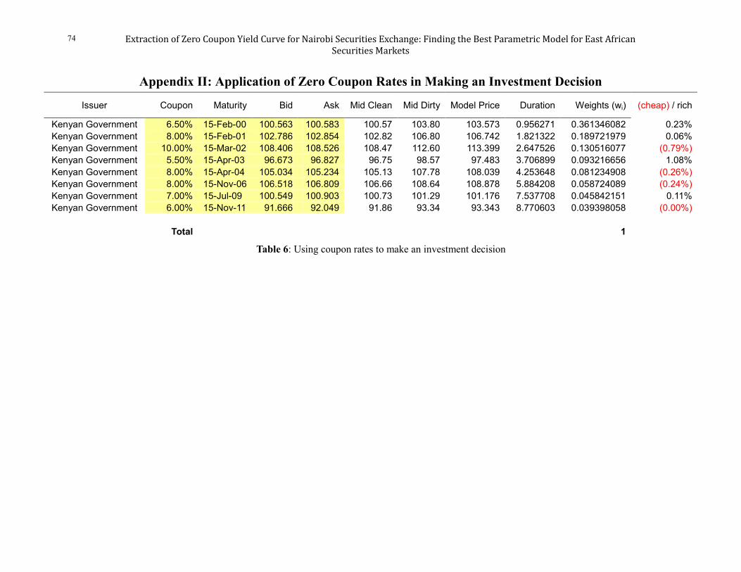
Appendix II: Application of Zero Coupon Rates in Making an Investment Decision

Issuer Coupon Maturity Bid Ask Mid Clean Mid Dirty Model Price Duration Weights (wi) (cheap) / rich

Kenyan Government 6.50% 15-Feb-00 100.563 100.583 100.57 103.80 103.573 0.956271 0.361346082 0.23% Kenyan Government 8.00% 15-Feb-01 102.786 102.854 102.82 106.80 106.742 1.821322 0.189721979 0.06% Kenyan Government 10.00% 15-Mar-02 108.406 108.526 108.47 112.60 113.399 2.647526 0.130516077 (0.79%) Kenyan Government 5.50% 15-Apr-03 96.673 96.827 96.75 98.57 97.483 3.706899 0.093216656 1.08% Kenyan Government 8.00% 15-Apr-04 105.034 105.234 105.13 107.78 108.039 4.253648 0.081234908 (0.26%) Kenyan Government 8.00% 15-Nov-06 106.518 106.809 106.66 108.64 108.878 5.884208 0.058724089 (0.24%) Kenyan Government 7.00% 15-Jul-09 100.549 100.903 100.73 101.29 101.176 7.537708 0.045842151 0.11% Kenyan Government 6.00% 15-Nov-11 91.666 92.049 91.86 93.34 93.343 8.770603 0.039398058 (0.00%)

Total 1

Table 6: Using coupon rates to make an investment decision

Documents

Extraction of Zero Coupon Yield Curve for Nairobi …1999), Maria (2009), Gilli (2010), Rezende (2011), Rosadi (2011), among others. This paper aims to estimate the Kenyan government