Applied Mathematics and Computation 219 (2012) 2260–2266

Contents lists available at SciVerse ScienceDirect

Applied Mathematics and Computation

journal homepage: www.elsevier .com/ locate /amc

Extrema of Young’s modulus in hexagonal materials

R.A. Khan ⇑, F. AhmadCentre for Advanced Mathematics and Physics, National University of Sciences and Technology, Sector H-12, Islamabad, Pakistan

a r t i c l e i n f o a b s t r a c t

Keywords:Young’s modulusElastic materialExtreme valuesHexagonal materials

0096-3003/$ - see front matter � 2012 Elsevier Inchttp://dx.doi.org/10.1016/j.amc.2012.08.072

⇑ Corresponding author.E-mail address: riaz_maths@yahoo.com (R.A. Kh

The optimum values of Young’s modulus for hexagonal materials are obtained by usingthe representation of the elasticity tensor by Ahmad and Khan [F. Ahmad, R.A. Khan,Eigenvectors of a rotation matrix, Q. J. Mech. Appl. Math. 62 (2009) 297–310]. Theexpression of Young’s modulus EðnÞ for a hexagonal material is written in terms of n3

only such that it reveals an axis of rotational symmetry in the direction x3, which is per-pendicular to the transverse isotropy plane, that is x1x2-plane: indeed the componentsn1;n2 of the unit vector n have no influence on the value of Young’s modulus. MoreoverYoung’s modulus is expressed in terms of invariant quantities, i.e. eigenvalues rather thancomponents of the compliance tensor. The problem is solved in a simple manner and isapplied to some real materials.

� 2012 Elsevier Inc. All rights reserved.

1. Introduction

Young’s modulus is a material property that describes the stiffness of an elastic material. It is defined as the ratio of uni-axial stress applied along the direction of a unit vector n to the longitudinal strain in the direction n. It is one of the mostimportant properties in engineering design.

Saint-Venant [1] was the first who studied the variation of Young’s modulus EðnÞ with the direction n. He constructed athree dimensional surface in which Young’s modulus was represented as the radial distance from a fixed origin in the direc-tion n to the surface. Rabinovich [2] called the three dimensional surface as the direction surface. In case of isotropic mate-rial, the direction surface is a sphere because in that case, it is independent of the direction n. Ting [3] has also shown that thedirection surface, for certain anisotropic (orthotropic and hexagonal) materials, is a sphere. Cazzani and Rovati [4] have ex-pressed Young’s modulus for cubic and hexagonal materials in terms of elastic compliances and they found explicitly thestationary values of EðnÞ and presented the direction surfaces of EðnÞ graphically for several materials. Ting [3] has also foundexplicit expression of the direction n and the stationary values of Young’s modulus for anisotropic materials. They also ob-tained these explicit expressions of Young’s modulus for hexagonal materials in terms of elastic compliances and discussedits direction surfaces. Unlike the approach of Ting and Cazaani and Rovati, Norris [5] has expressed Young’s modulus in termof invariant quantities, i.e. in terms of eigenvalues and discussed its extreme values. He also considered Poisson’s ratio incubic materials. He found evidence for Poisson’s ratio less than �1 in a certain direction and greater than 2 in some otherdirection. In this paper we have expressed Young’s modulus in terms of eigenvalues rather than in terms of componentsof the compliance tensor which are not invariant quantities. Additionally, we have used the representation derived for a hex-agonal material in [6] to find an expression for EðnÞ and then found its optimum values. We have also expressed the Young’smodulus, EðnÞ, for a hexagonal material in terms of one variable, n3, only. Hence the problem is solved in a simple manner.

In Section 2, the Young’s modulus for cubic materials is investigated. We have discussed the problem considered by Norris[5] in detail and reformulated it in six dimensions by applying the representation derived for a cubic material [6] to find an

. All rights reserved.

an).

R.A. Khan, F. Ahmad / Applied Mathematics and Computation 219 (2012) 2260–2266 2261

expression for EðnÞ. In Section 3, the extreme values of Young’s modulus are discussed. The results obtained in Section 3 areillustrated by some examples of real materials in Section 4.

2. Cubic materials

Norris used a result of Walpole [7] to express the compliance tensor s for a cubic material in the form

s ¼ 13k

J þ 12l1ðI � DÞ þ 1

2l2ðD� JÞ; ð2:1Þ

where

Iijkl ¼12ðdikdjl þ dildjkÞ;

Jijkl ¼13

dijdkl;

Dijkl ¼ di1dj1dk1dl1 þ di2dj2dk2dl2 þ di3dj3dk3dl3:

ð2:2Þ

The parameters k;l1;l2 are related to the Voigt notation for the stiffness tensor as follows

k ¼ c11 þ 2c12

3; l1 ¼ c44; l2 ¼

c11 � c12

2; ð2:3Þ

i.e. 3k;2l1 and 2l2 are eigenvalues of the elasticity tensor in the Cowin–Mehrabadi formalism [8]. Young’s modulus in thedirection specified by a unit vector n ¼ ðn1;n2;n3ÞT is defined by

EðnÞ ¼ 1sijklninjnknl

;

or

1EðnÞ ¼ sijklninjnknl: ð2:4Þ

Let

n22n2

3 þ n23n2

1 þ n21n2

2 ¼ FðnÞ; ð2:5Þ

Substituting (2.3) and (2.5) into (2.4) and using n21 þ n2

2 þ n23 ¼ 1, we have

1EðnÞ ¼ s11 � 2s11FðnÞ þ 1

l1þ 2s12

� �FðnÞ ¼ s11 �

1l2

FðnÞ þ 1l1

FðnÞ:

The value of s11 in terms of k and l2 can be found as

s11 ¼1

9kþ 1

3l2

Thus 1EðnÞ has the following form

1EðnÞ ¼

19kþ 1

3l2� 1

l2FðnÞ þ 1

l1FðnÞ ¼ 1

9kþ 1

3l2� 1

l2� 1

l1

� �FðnÞ; ð2:6Þ

which is the result derived by Norris [5].It is easy to show that

0 6 F 613

ð2:7Þ

From (2.6) it is clear that, if 1l1

P 1l2

then

max1E¼ 1

9kþ 1

3l1;

min1E¼ 1

9kþ 1

3l2:

2262 R.A. Khan, F. Ahmad / Applied Mathematics and Computation 219 (2012) 2260–2266

Also if 1l16

1l2

then

max1E¼ 1

9kþ 1

3l2;

min1E¼ 1

9kþ 1

3l1:

Hayes and Shuvalov [9] and Cazzani and Rovati [4] have also obtained the above results but they have expressed 1E in terms of

components of the compliance tensor rather than the invariant expressions used above. Now we shall obtain (2.6) by therepresentation of c for a cubic material in [6]. They have shown that the elasticity tensor may be represented as

c ¼ k1F1 þ k2F2 þ k4F3:

Hence the compliance tensor becomes

s ¼ 1k1

F1 þ1k2

F2 þ1k4

F3;

where F1; F2 and F3 are

F1 ¼13

1 1 1 0 0 0

1 1 1 0 0 0

1 1 1 0 0 0

0 0 0 0 0 0

0 0 0 0 0 0

0 0 0 0 0 0

0BBBBBBBBBBBB@

1CCCCCCCCCCCCA; F2 ¼

13

2 �1 �1 0 0 0

�1 2 �1 0 0 0

�1 �1 2 0 0 0

0 0 0 0 0 0

0 0 0 0 0 0

0 0 0 0 0 0

0BBBBBBBBBBBB@

1CCCCCCCCCCCCAand F3 ¼

0 0 0 0 0 0

0 0 0 0 0 0

0 0 0 0 0 0

0 0 0 1 0 0

0 0 0 0 1 0

0 0 0 0 0 1

0BBBBBBBBBBBB@

1CCCCCCCCCCCCA:

Young’s modulus in the above six dimensional formalism is given by

1EðnÞ ¼ sij

bNibNj;

where for n ¼ ðn1;n2;n3ÞT ; bN ¼ ðn21;n

22;n

23;

ffiffiffi2p

n2n3;ffiffiffi2p

n3n1;ffiffiffi2p

n1n2ÞT . To calculate Young’s modulus, we simply need to findbNT sbN. That is

1EðnÞ ¼

1k1

bNT F1bN þ 1

k2

bNT F2bN þ 1

k4

bNT F3bN ¼ 1

3k1þ 2

3k2þ 2

1k4� 1

k2

� �FðnÞ: ð2:8Þ

This is identical to (2.6) if we identify k1 ¼ 3k, k2 ¼ 2l2 and k4 ¼ 2l1. Thus our formulation gives the same results as those ofNorris [5] and Cazzani and Rovati [4]. Next we shall use results of Ahmad and Khan [6] to express Young’s modulus in termsof eigenvalues of the elasticity tensor and an arbitrary parameter.

3. Transversely isotropic (hexagonal) materials

Ahmad and Khan [6] have shown that the elasticity tensor for transversely isotropic (hexagonal) materials may be rep-resented as

c ¼ k1E1 þ k2E2 þ k3ðE3 þ E4Þ þ k5ðE5 þ E6Þ: ð3:1Þ

Hence the compliance tensor becomes

s ¼ 1k1

E1 þ1k2

E2 þ1k3ðE3 þ E4Þ þ

1k5ðE5 þ E6Þ ð3:2Þ

where E1; E2; E3 þ E4 and E5 þ E6 are

E1 ¼1

2þ a2

1 1 a 0 0 0

1 1 a 0 0 0

a a a2 0 0 0

0 0 0 0 0 0

0 0 0 0 0 0

0 0 0 0 0 0

0BBBBBBBBBBBB@

1CCCCCCCCCCCCA; E2 ¼

14þ 2a2

a2 a2 �2a 0 0 0

a2 a2 �2a 0 0 0

�2a �2a 4 0 0 0

0 0 0 0 0 0

0 0 0 0 0 0

0 0 0 0 0 0

0BBBBBBBBBBBB@

1CCCCCCCCCCCCA;

R.A. Khan, F. Ahmad / Applied Mathematics and Computation 219 (2012) 2260–2266 2263

E3 þ E4 ¼

12 � 1

2 0 0 0 0

� 12

12 0 0 0 0

0 0 0 0 0 0

0 0 0 0 0 0

0 0 0 0 0 0

0 0 0 0 0 1

0BBBBBBBBB@

1CCCCCCCCCAand E5 þ E6 ¼

0 0 0 0 0 0

0 0 0 0 0 0

0 0 0 0 0 0

0 0 0 1 0 0

0 0 0 0 1 0

0 0 0 0 0 0

0BBBBBBBBB@

1CCCCCCCCCA:

By using the above expressions, we can calculate 1EðnÞ ¼ bNT sbN as follows:

1EðnÞ ¼

bNT sbN ¼ 1k1

bNT E1bN þ 1

k2

bNT E2bN þ 1

k3

bNTðE3 þ E4ÞbN þ 1k5

bNTðE5 þ E6ÞbN¼ 1

k1

½1þ ða� 1Þn23�

2

2þ a2 þ 12k2

ðaþ 2Þn23 � a

� �2

2þ a2 þ 12k3ð1� n2

3Þ2 þ 2

k5n2

3ð1� n23Þ: ð3:3Þ

We note that if n3 ¼ 1, the Young’s modulus depends only on k1 and k2. In this direction

1EðnÞ ¼

1k1

a2

2þ a2 þ1k2

22þ a2 : ð3:4Þ

For a cubic material, 1EðnÞ, in a direction parallel to one of the coordinate axes, given by Eq. (2.8), becomes

1EðnÞ ¼

13k1þ 2

3k2:

We shall get the same result in the present case if we let a ¼ 1 in (3.4). Thus there exists a transversely isotropic materialclosest to a cubic material in this sense.

Eq. (3.3) is a function of n3 only, that is 1EðnÞ ¼ 1

Eðn3Þ. For convenience, we let

1Eðn3Þ

¼ f ðn3Þ: ð3:5Þ

To find the extremal direction, the derivative of f ðn3Þ with respect to n3 must be equal to zero. This gives

f 0ðn3Þ ¼4n3ða� 1Þ½1þ ða� 1Þn2

3�k1ð2þ a2Þ þ 2n3ðaþ 2Þ½ðaþ 2Þn2

3 � a�2

k2ð2þ a2Þ � 2n3ð1� n23Þ

k3þ 4n3ð1� 2n2

3Þk5

¼ 0:

From this we find

n3 ¼ 0;

or

1k3� 4

k5þ 2ða� 1Þ2

k1ð2þ a2Þ þðaþ 2Þ2

k2ð2þ a2Þ

!n2

3 ¼1k3� 2

k5� 2ða� 1Þ

k1ð2þ a2Þ þaðaþ 2Þ

k2ð2þ a2Þ ð3:6Þ

which leads to

n3 ¼ �p; say;

where,

p ¼

ffiffiffiffiffiffiffiffiffiffiffiffiffiffiffiffiffiffiffiffiffiffiffiffiffiffiffiffiffiffiffiffiffiffiffiffiffiffiffiffiffiffiffiffiffiffiffiffiffiffiffiffiffi1k3� 2

k5� 2ða�1Þ

k1ð2þa2Þ þaðaþ2Þ

k2ð2þa2Þ

1k3� 4

k5þ 2ða�1Þ2

k1ð2þa2Þ þðaþ2Þ2

k2ð2þa2Þ

:

vuuut ð3:7Þ

In order that n3 be real we require the following pairs of inequalities

1k2þ 1

k3� 2

k5þ 2ða� 1Þ

2þ a2

1k2� 1

k1

� �> 0; ð3:8aÞ

and

2k1þ 1

k2þ 1

k3� 4

k5þ 2ð2aþ 1Þ

2þ a2

1k2� 1

k1

� �> 0; ð3:8bÞ

or

1k2þ 1

k3� 2

k5þ 2ða� 1Þ

2þ a2

1k2� 1

k1

� �< 0; ð3:9aÞ

2264 R.A. Khan, F. Ahmad / Applied Mathematics and Computation 219 (2012) 2260–2266

and

2k1þ 1

k2þ 1

k3� 4

k5þ 2ð2aþ 1Þ

2þ a2

1k2� 1

k1

� �< 0: ð3:9bÞ

On the other hand, if neither (3.8a,b) nor (3.9a,b) are satisfied, the Young’s modulus will attain its extreme values in the planeof isotropy. But if (3.8a,b) or (3.9a,b) are satisfied, then we find the extreme values of Young’s modulus as follows:

The second derivative of f ðn3Þ with respect to n3 has the following expression

f 00ðn3Þ ¼4ð�1þ aþ 3n2

3 � 6an23 þ 3a2n2

3Þk1ð2þ a2Þ þ 2ð2þ aÞ½6n2

3 þ að3n23 � 1Þ�

k2ð2þ a2Þ þ 4n23 � 2ð1� n2

3Þk3

þ 4ð1� n23Þ � 20n2

3

k5ð3:10Þ

Now we substitute the value of n3 ¼ �p;0 into (3.10), respectively, we have

f 0ð�pÞ ¼ � 8ða� 1Þ2þ a2ð Þk1

þ 4að2þ aÞ2þ a2ð Þk2

þ 4k3� 8

k5¼ 4

1k2þ 1

k3� 2

k5

� �þ 2

a� 12þ a2

1k2� 1

k1

� �� �ð3:11Þ

Note that the right hand side of (3.11) is identical, except for a factor of 4, to the left hand side of (3.8a). Also

f 00ð0Þ ¼ 4ða� 1Þ2þ a2ð Þk1

þ 2að2þ aÞ2þ a2ð Þk2

� 2k3þ 4

k5¼ �2

1k2þ 1

k3� 2

k5

� �þ 2

a� 12þ a2

1k2� 1

k1

� �� �ð3:12Þ

We note that

f 00ð0Þ ¼ �12

f 00ð�pÞ:

From the above equations, we conclude the following.

(i) If conditions (3.8) are satisfied then there is a minimum of 1EðnÞ in the direction n3 ¼ �p and a maximum when n3 ¼ 0 i.e.

in the plane of isotropy.(ii) If conditions (3.9) are satisfied then there is a maximum of 1

EðnÞ in the direction n3 ¼ �p and a minimum when n3 ¼ 0i.e. in the plane of isotropy.

(iii) When neither (3.8) nor (3.9) are satisfied, there is no maximum or minimum in any direction not lying in the plane ofisotropy.

4. Applications to some real materials

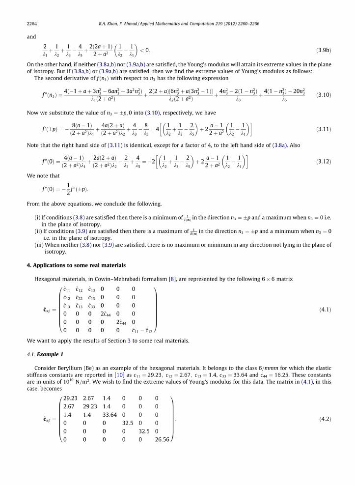
Hexagonal materials, in Cowin–Mehrabadi formalism [8], are represented by the following 6� 6 matrix

cab ¼

c11 c12 c13 0 0 0c12 c22 c13 0 0 0c13 c13 c33 0 0 00 0 0 2c44 0 00 0 0 0 2c44 00 0 0 0 0 c11 � c12

0BBBBBBBB@

1CCCCCCCCAð4:1Þ

We want to apply the results of Section 3 to some real materials.

4.1. Example 1

Consider Beryllium (Be) as an example of the hexagonal materials. It belongs to the class 6=mmm for which the elasticstiffness constants are reported in [10] as c11 ¼ 29:23; c12 ¼ 2:67; c13 ¼ 1:4, c33 ¼ 33:64 and c44 ¼ 16:25. These constantsare in units of 1010 N=m2. We wish to find the extreme values of Young’s modulus for this data. The matrix in (4.1), in thiscase, becomes

cab ¼

29:23 2:67 1:4 0 0 02:67 29:23 1:4 0 0 01:4 1:4 33:64 0 0 00 0 0 32:5 0 00 0 0 0 32:5 00 0 0 0 0 26:56

0BBBBBBBB@

1CCCCCCCCA: ð4:2Þ

R.A. Khan, F. Ahmad / Applied Mathematics and Computation 219 (2012) 2260–2266 2265

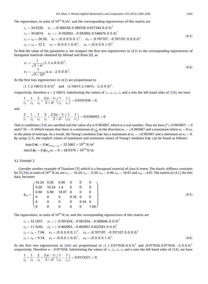
The eigenvalues, in units of 1010 N=m2, and the corresponding eigenvectors of this matrix are

k1 ¼ 34:9326; v1 ¼ ð0:386558; 0:386558;0:837344;0;0;0ÞT

k2 ¼ 30:6074; v2 ¼ ð�0:592092;�0:592092;0:546676;0;0;0ÞT

k3 ¼ k4 ¼ 26:56; v3 ¼ ð0;0; 0;0; 0;1ÞT ; v4 ¼ ð0:707107;�0:707107;0;0;0;0ÞT

k5 ¼ k6 ¼ 32:5; v5 ¼ ð0;0;0;1;0;0ÞT ; v6 ¼ ð0;0;0;0;1;0ÞT :

ð4:3Þ

To find the value of the parameter a, we compare the first two eigenvectors in (4.3) to the corresponding eigenvectors ofhexagonal materials obtained by Ahmad and Khan [6], as

v1 ¼1ffiffiffiffiffiffiffiffiffiffiffiffiffiffi

2þ a2p ð1;1; a;0; 0;0ÞT ;

v2 ¼1ffiffiffiffiffiffiffiffiffiffiffiffiffiffiffiffiffi

4þ 2a2p ða; a;�2; 0;0; 0ÞT :

ð4:4Þ

As the first two eigenvectors in (4.3) are proportional to

ð1;1;2:16615;0;0;0ÞT and ð2:16615;2:16615;�2;0;0;0ÞT ;

respectively, therefore a ¼ 2:16615. Substituting the values of k1; k2; k3; k5 and a into the left hand sides of (3.8), we have

1k2þ 1

k3� 2

k5þ 2ða� 1Þ

2þ a2

1k2� 1

k1

� �¼ 0:0101938 > 0;

and

2k1þ 1

k2þ 1

k3� 4

k5þ 2ð2aþ 1Þ

2þ a2

1k2� 1

k1

� �¼ 0:0109452 > 0:

That is conditions (3.8) are satisfied and the value of p is 0:965067, which is a real number. Thus we have f 00ð�0:965067Þ > 0and f 00ð0Þ < 0. Which means that there is a minimum of 1

EðnÞ in the direction n3 ¼ �0:965067 and a maximum when n3 ¼ 0 i.e.

in the plane of isotropy. As a result, the Young’s modulus EðnÞ has a maximum at n3 ¼ �0:965067 and a minimum at n3 ¼ 0.By using (3.3), the explicit values of maximum and minimum values of Young’s modulus EðnÞ can be found as follows:

max EðnÞ ¼ EðnÞjat n3¼�p ¼ 33:5461� 1010 N=m2

min EðnÞ ¼ EðnÞjat n3 ¼ 0 ¼ 28:9379� 1010 N=m:

4.2. Example 2

Consider another example of Titanium (Ti) which is a hexagonal material of class 6=mmm. The elastic stiffness constantsfor Ti [10], in units of 1010 N=m, are c11 ¼ 16:24; c12 ¼ 9:20; c13 ¼ 6:90; c33 ¼ 18:07 and c44 ¼ 4:67. The matrix in (4.1), for thisdata, becomes

cab ¼

16:24 9:20 6:90 0 0 09:20 16:24 1:4 0 0 06:90 6:90 18:07 0 0 00 0 0 9:34 0 00 0 0 0 9:34 00 0 0 0 0 7:04

0BBBBBBBB@

1CCCCCCCCA: ð4:5Þ

The eigenvalues, in units of 1010 N=m, and the corresponding eigenvectors of this matrix are

k1 ¼ 32:1857; v1 ¼ ð�0:581654;�0:581654;�0:568646;0;0;0ÞT

k2 ¼ 11:3243; v2 ¼ ð�0:402093;�0:402093;0:822583;0;0;0ÞT

k3 ¼ k4 ¼ 7:04; v3 ¼ ð0;0; 0;0;0;1ÞT ; v4 ¼ ð0:707107;�0:707107;0;0;0;0ÞT

k5 ¼ k6 ¼ 9:34; v5 ¼ ð0; 0;0;1;0;0ÞT ; v6 ¼ ð0; 0;0;0;1;0ÞT : ð4:6Þ

As the first two eigenvectors in (4.6) are proportional to ð1;1;0:977636;0;0;0ÞT and ð0:977636;0:977636;�2;0;0;0ÞT

respectively. Therefore a ¼ 0:977636. Substituting the values of k1; k2; k3; k5 and a into the left hand sides of (3.8), we have

1k2þ 1

k3� 2

k5þ 2ða� 1Þ

2þ a2

1k2� 1

k1

� �¼ 0:0153521 > 0;

2266 R.A. Khan, F. Ahmad / Applied Mathematics and Computation 219 (2012) 2260–2266

and

2k1þ 1

k2þ 1

k3� 4

k5þ 2ð2aþ 1Þ

2þ a2

1k2� 1

k1

� �¼ �0:0213227 < 0:

As neither (3.8) nor (3.9) are satisfied, therefore no real value of p exists. Thus for Titanium (Ti), there is no maximum orminimum of Young’s modulus in any direction not lying in the plane of isotropy.

Also Eq. (3.12) gives

f 00ð0Þ ¼ �0:0307044 < 0:

Therefore 1EðnÞ jat n3¼0 ¼ 0:958114 is a maximum in any direction in the plane of isotropy. It has no minimum in any direction.

Finally, we conclude that the minimum value of Young’s modulus EðnÞ in any direction in the plane of isotropy, i.e. n3 ¼ 0 is

min EðnÞ ¼ EðnÞjat n3¼0 ¼ 1:043� 1010 N=m

but Young’s modulus has no maximum in any direction.

Acknowledgments

Financial support was provided to the first author by the National University of Sciences and Technology, Islamabad,Pakistan and to the second author by the Higher Education Commission of Pakistan.

References

[1] B. Saint-Venant, Memoire sur la Distribution des elasticities, J. Math. Pures er Appl. (Liouville) II 10 (1863) 297–349.[2] A.L. Rabinovich, On the elastic constants and strenth of aircraft materials, Trudy Trentr. Aero-gidvodin 582 (1946) 1–56.[3] T.C.T. Ting, Explicit expression for the stationary values of Young’s modulus and the shear modulus for anisotropic elastic materials, J. Mech. (formerly

the Chinese J. Mech. Ser. A) 21 (4) (2005) 255–266.[4] A. Cazzani, M. Rovati, Extrema of Young’s modulus cubic and transversely isotropic solids, Int. J. Solids Struct. 40 (2003) 1713–1744.[5] A.N. Norris, Poisson’s ratio in cubic materials, Proc. R. Soc. A 462 (2006) 3385–3405.[6] F. Ahmad, R.A. Khan, Eigenvectors of a rotation matrix, Q. J. Mech. Appl. Math 62 (2009) 297–310.[7] L.J. Walpole, Fourth-rank tensors of the thirty-two crystal classes: multiplication tables, Proc. R. Soc. Lond. A 391 (1984) 149–179.[8] M.M. Mehrabadi, S.C. Cowin, Eigentensors of linear anisotropic elastic materials, Q. J. Mech. Appl. Math. 43 (1990) 15–41.[9] M. Hayes, A. Shuvalov, On the extreme values of Young and Poisson’s ratio for cubic materials, J. Appl. Mech. 65 (3) (1998).

[10] E. Dieulesaint, D. Royer, Elastic Waves in Solids I: Free and Guided Propagation, Springer-Verlag, Berlin Heidelberg, 2000.