EXTREME VALUE ANALYSIS: STILL WATER LEVEL

EXTREME VALUE ANALYSIS: STILL WATER LEVEL

by

Sofia Caires

2011

JCOMM Technical Report No. 58

WORLD METEOROLOGICAL ORGANIZATION

_____________

INTERGOVERNMENTAL OCEANOGRAPHIC COMMISSION (OF UNESCO)

___________

EXTREME VALUE ANALYSIS: STILL WATER LEVEL

by

Sofia Caires

2011

JCOMM Technical Report No. 58

N O T E The designations employed and the presentation of material in this publication do not imply the expression of any opinion whatsoever on the part of the Secretariats of the Intergovernmental Oceanographic Commission (of UNESCO), and the World Meteorological Organization concerning the legal status of any country, territory, city or area, or of its authorities, or concerning the delimitation of its frontiers or boundaries.

Extreme value analysis i

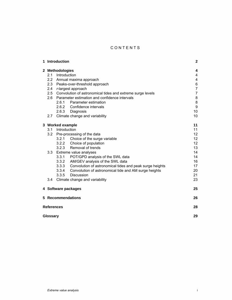
C O N T E N T S

1 Introduction 2

2 Methodologies 4 2.1 Introduction 4 2.2 Annual maxima approach 4 2.3 Peaks-over-threshold approach 6 2.4 r-largest approach 7 2.5 Convolution of astronomical tides and extreme surge levels 7 2.6 Parameter estimation and confidence intervals 8

2.6.1 Parameter estimation 8 2.6.2 Confidence intervals 9 2.6.3 Diagnosis 10

2.7 Climate change and variability 10

3 Worked example 11 3.1 Introduction 11 3.2 Pre-processing of the data 12

3.2.1 Choice of the surge variable 12 3.2.2 Choice of population 12 3.2.3 Removal of trends 13

3.3 Extreme value analyses 14 3.3.1 POT/GPD analysis of the SWL data 14 3.3.2 AM/GEV analysis of the SWL data 16 3.3.3 Convolution of astronomical tides and peak surge heights 17 3.3.4 Convolution of astronomical tide and AM surge heights 20 3.3.5 Discussion 21

3.4 Climate change and variability 23

4 Software packages 25

5 Recommendations 26

References 28

Glossary 29

Extreme value analysis 2

Introduction Still water level (SWL) is the level that the sea surface (at a given point and time) would adopt in the absence of wind waves. SWLs are influenced by astronomical and meteorological effects and given by the combination of the astronomical tide and the storm surge. Estimates of the m-year return value of SWL─the value which is exceeded on average once every m years─are needed for the design and control of water defences, and for the mapping of flood risk areas. In the control of the safety of the Netherlands sea defences return values of up to 1/10,000-yr are used. In the mapping of flood risk areas in the United Kingdom 1/1,000-yr return values are used. The longer time series of SWL data available usually cover at most 100 years, meaning that one generally needs to extrapolate well beyond the range of the available data. Although the tide is a deterministic process, the surge process is non-deterministic, making the estimation of SWL extremes a statistical problem.

Since the tragic North Sea flood of 1953, in which more than 1800 people died in the Netherlands and 300 in the United Kingdom, a lot of attention has been given to flood defence and estimation. The statistical estimation of SWL return values has been extensively studied in the beginning of the 90’s separately in the Netherlands and in the United Kingdom by teams including two well-known extreme value theory specialists: Prof. Laurens de Haan (Dillingh et al., 1993) in the Netherlands and Prof. Jonathan Tawn (Dixon and Tawn, 1994 and Dixon et al., 1998) in the United Kingdom. They have laid the basis for extreme value analyses of SWL.

One of the following three approaches is usually considered to determine return values of SWL:

1. Extreme value analysis of the SWLs. 2. Estimation of extreme water levels from the convolution of the extreme value

distribution of the (synchronous) surge (or that of the skew surge, a non-synchronous difference between SWL and tide) with the empirical distribution of tidal levels. Compared to 1., this is thought to make better use of scarce data, by allowing the use of available complete tidal information.

3. Estimation of extreme surge levels from extreme weather conditions (winds and atmospheric pressures) and computation of pessimistic or conservative SWL estimates by adding the Highest Astronomical Tide to them.

In this report, approaches 1. and 2. will be assessed and guidelines provided as to which should be used in a given situation. In each approach, two different extreme value analysis methods will be considered: the peaks-over-threshold and annual maxima methods. Using the results of our analyses with Approach 2., we shall also provide indications about the tidal level that should be used in Approach 3.

Besides a decision about which approach to take, a decision must also be made about which offset/surge to be used in Approach 2; this depends on the location of the data.


In this report we begin by describing and discussing approaches based on extreme value theory that can be used to estimate return values of SWL in Chapter 2. We then present in Chapter 3 a worked example using a long-term time series of still water level measurements processed and quality-checked by the Dutch Ministry of Transport, Public Works and Water Management. They are the measurements of the gauge located at Hoek van Holland, The Netherlands (see Figure 3.1), available from 1887 onwards. In Chapter 4 we provide an inventory of software packages available to carry out extreme value analyses. We finish in Chapter 5 with some guidelines / recommendations.


Methodologies

Introduction

In the framework of approaches 1. and 2. outlined in the Introduction, different paths of analysis can be followed. For example, in both cases three different methods of extreme value analysis may be used: the annual maxima, the peaks-over-threshold or the r-largest method. This chapter briefly introduces the principles of extreme value theory and describes these methods in sections 2.2, 2.3 and 2.4. For further background information on extreme value theory and analyses we recommend the book of Stuart Coles (Coles, 2001), which is comprehensive, easy to read and presents many applications to environmental data.

For a given method of extreme value analysis, Approach 2. consists of

1. separating the astronomic tide from the water level observations, 2. analysing the astronomic tide and the residual (storm surge) separately, 3. computing the empirical distribution of the astronomic tide, 4. carrying out a univariate extreme value analysis of the storm surge data, and 5. computing the convolution of the empirical distribution of the astronomic tide with the

extreme value distribution estimated from the storm surge data (a particular example of joint probability techniques).

In the worked example to be presented here we consider data for which the tide and the residual signals have already been separated. Harmonic analysis of the still water levels is a problem in itself and will not be considered here. Section 2.5 describes the computation of the convolution needed in step 5 above.

The estimation of model parameters and the computation of confidence intervals are based on the same methods in all the extreme value analyses; they are described in Section 2.6.

Annual maxima approach Extreme value theory provides analogues of the central limit theorem for the extreme values in a sample. According to the central limit theorem, the mean of a large number of random variables, irrespective of the distribution of each variable, is distributed approximately according to a Gaussian distribution. According to extreme value theory, the extreme values in a large sample have an approximate distribution that is independent of the distribution of each variable.

In order to explain the basic ideas (see e.g. Leadbetter et al., 1983, for more details), let us define { }1max , ,n nM X X= K , where 1 2,X X K is a sequence of independent random variables having a common distribution function F. In its simplest form, the extremal types theorem states the following: If there exist sequences of constants { }0nσ > and { }nμ such

that { }P ( )n n nM z G zσ μ+ ≤ → as n →∞ , where G is a non-degenerate cumulative


distribution function, then G must be a generalized extreme value (GEV) distribution, which is given by

1

exp 1 , for 0

( )

exp exp , for 0,

z

G zz

ξμξ ξ

σ

μ ξσ

−⎧ ⎧ ⎫⎡ ⎤−⎪ ⎪⎛ ⎞⎪ − + ≠⎨ ⎬⎜ ⎟⎢ ⎥⎝ ⎠⎪ ⎣ ⎦⎪ ⎪⎩ ⎭= ⎨⎧ ⎫⎪ ⎡ ⎤−⎛ ⎞− − =⎨ ⎬⎪ ⎜ ⎟⎢ ⎥⎝ ⎠⎣ ⎦⎩ ⎭⎩

(2.1)

where z take values in three different sets according to the sign of ξ: z μ σ ξ> − if 0ξ > (the domain of z has a lower bound), z μ σ ξ< − if 0ξ < (the domain of z has an upper bound), and z−∞ < < ∞ if 0ξ = .

In other words, if the distribution function of (a normalization of) the maximum value in a random sample of size n converges to a distribution function as n tends to infinity, then that distribution function must be a GEV distribution. Moreover, this and other results of extreme value theory hold true even under general dependence conditions (Coles, 2001).

In Eq. (2.1), the parameters μ, σ and ξ are called the location, scale, and shape parameters and satisfy μ−∞ < < ∞ , 0σ > and ξ−∞ < < ∞ . For 0ξ = the GEV is the Gumbel distribution, for 0ξ > it is the Fréchet distribution, and for 0ξ < it is the Weibull distribution. For 0ξ > the tail of the GEV is “heavier” (i.e., decreases more slowly) than the tail of the Gumbel distribution, and for 0ξ < it is “lighter” (decreases more quickly and actually reaches 0) than that of the Gumbel distribution. The GEV is said to have a type II tail for 0ξ > and a type III tail for 0ξ < 1. The tail of the Gumbel distribution is called a type I tail.

The extremal types theorem gives rise to the annual maxima (AM) method of modelling extremes, in which the GEV distribution is fitted to a sample of block maxima (e.g. to annual maxima, though biannual, monthly or even daily maxima can of course be used as well).

One of the main applications of extreme value theory is the estimation of the once per m year (1/m-yr) return value, the value which is exceeded on average once every m years. The 1/m-yr return value based on the AM method/GEV distribution, mz , is given by

-11 log 1 , for 0m

1log log 1 , for 0.m

mz

ξσμ ξξ

μ σ ξ

⎧ ⎛ ⎞⎧ ⎫⎛ ⎞⎪ ⎜ ⎟− − − − ≠⎨ ⎬⎜ ⎟⎜ ⎟⎝ ⎠⎪ ⎩ ⎭⎝ ⎠= ⎨⎪ ⎧ ⎫⎛ ⎞− − − =⎨ ⎬⎪ ⎜ ⎟

⎝ ⎠⎩ ⎭⎩

1. Please note that some articles (e.g. Hosking and Wallis, 1987) use another convention for the

sign of the shape parameter: a negative shape parameter in those references corresponds to a type II distribution.


The sample sizes of annual maxima data are usually small, so that model estimates, especially return values, have large uncertainties. This has motivated the development of more sophisticated methods that enable the modelling of more data than just block maxima. These methods are based on two well-known characterizations of extreme value distributions: one based on exceedances of a threshold, and the other based on the behaviour of the r largest (for small values of r) observations within a block. These are described in the following two sections.

Peaks-over-threshold approach

The approach based on the exceedances of a high threshold, hereafter referred to as the POT (Peaks-over-threshold) method, consists of fitting the generalized Pareto distribution (GPD) to the peaks of clustered excesses over a threshold, the excesses being the observations in a cluster minus the threshold, and calculating return values by taking into account the rate of occurrence of clusters (see Pickands, 1971 and 1975, and Davidson and Smith, 1990). Under very general conditions this procedure ensures that the data can have only three possible, albeit asymptotic, distributions (the three forms of the GPD given below) and, moreover, that observations belonging to different peak clusters are (approximately) independent. In the POT method, the peak excesses over a high threshold u of a time series are assumed to occur in time according to a Poisson process with rate uλ and to be independently distributed with a GPD, whose distribution function is given by

1

1 1 , for 0( )

1 exp , for 0,u

y

F yy

ξ

ξ ξσ

ξσ

−⎧ ⎛ ⎞− + ≠⎪ ⎜ ⎟⎪ ⎝ ⎠= ⎨⎛ ⎞⎪ − − =⎜ ⎟⎪ ⎝ ⎠⎩

%

%

where 0 y< < ∞ , 0σ >% and ξ−∞ < < ∞ . The two parameters of the GPD are called the scale (σ% ) and shape (ξ) parameters. When 0ξ = the GPD is said to have a type I tail and amounts to the exponential distribution with mean σ% ; when 0ξ > it has a type II tail and it is the Pareto distribution; and when 0ξ < it has a type III tail and it is a special case of the beta distribution. If 0ξ < , just as with the GEV, the support of the GPD was an upper-bound, σ ξ− % , which is called the upper end-point of the GPD. The significance of this upper end-point is that the excesses over u modelled by the GPD cannot take values greater than uσ ξ− , which in turn means that the exceedances of the variable of interest cannot exceed the value

*ux u σ ξ= − . This parameter *x is to be thought of as the upper-limit of the variable of

interest (e.g. of SWL).

The 1/m-yr return value based on a POT/GPD analysis, zm, is given by

u

u

{ ( m) 1}, for 0

log( m), for 0.m

uz

u

ξσ λ ξξσ λ ξ

⎧ + − ≠⎪= ⎨⎪ + =⎩

%

%

Just as block maxima have the GEV as their approximate distribution, the threshold excesses have a corresponding approximate distribution within the GPD. Moreover, the parameters of


the GPD of threshold excesses are uniquely determined by those of the associated GEV distribution of block maxima. In particular, the shape parameter is the same, and the scale parameters of the two distributions are related by ( )uσ σ ξ μ= + −% .

The choice of threshold (analogous to the choice of block size in the block maxima approach) represents a trade off between bias and variance: too low a threshold is likely to violate the asymptotic basis of the model, leading to bias; too high a threshold will generate fewer excesses with which to estimate the model, leading to high variance. An important property of the POT/GPD approach is the threshold stability property: if a GPD is a reasonable model for excesses of a threshold 0u , then for a higher threshold u a GPD should also apply; the two GPD’s have identical shape parameter and their scale parameters are related by

( )0 0u u u uσ σ ξ= + −% % , which can be reparameterized as

*uσ σ ξμ= −% . (2.2)

Consequently, if μ0 is a valid threshold for excesses to follow the GPD then estimates of both σ* and ξ should remain nearly constant above μ0. This property of the GPD can be used to find the minimum threshold at which a GPD model applies to the data.

r-largest approach

The characterizations of extreme value distributions based on the behaviour of the r largest observations within a block is known as the r-largest approach. This approach is generally thought to be less efficient than the peaks-over-threshold approach (see Coles, 2001) and is not considered in detail here.

Briefly, it consists of collecting the r-largest values per year (instead of merely the annual maxima) and fitting the r-largest distribution (see, for instance, Coles, 2001, pp. 68) to the data. Extensive examples of the application of this method to estimate return values of SWL are given by Dixon and Tawn (1994).

The choice of r is analogous to the choice of threshold in the POT method and the choice of block size in the block maxima approach.

Convolution of astronomical tides and extreme surge levels Extreme value analyses based on the SWL alone, especially when the available time series are short, are considered by some to be wasteful of data. In order to take advantage of the sometimes fully available tidal information, extreme values of SWLs can also be estimated from the convolution of the distribution of the residual (the synchronous or non- synchronous


offset/setup/surge)2 extremes and the empirical distribution of the tidal levels. More precisely, given that the SWL is the sum of the residual and the tide and that these variables can, under certain conditions, be assumed independent, another approach to obtaining the extreme value distribution of the SWL is to estimate the distribution function of ‘large values’ of SWL by the convolution integral

( ) ( ) ( )rF z G z x f x dx= −∫ where Gr is the distribution function of ‘large values’ of the residual (either the GPD or the GEV) and f is the (in principle fully known) density function of the tide levels.

If Gr is the GPD, the 1/m-yr return value of SWL can be computed from F by finding zm such that 1 ( ) 1/( )F z mλ− = , where λ has been defined in Section 2.3. If Gr is the GEV, the 1/m yr return value is computed by solving the same equation with λ replaced by 1.

The extension of this approach to dependent variables is given in Dixon and Tawn (1994).

Parameter estimation and confidence intervals

Parameter estimation There are several methods available for the estimation of the parameters of extreme value distributions. Most of them, for instance the methods of moments and of probability weighted moments, give explicit expressions for the parameter estimates. The maximum likelihood (ML) method tends to be the preferred estimation method since it is quite general and more flexible than other methods, especially when the number of parameters is increased as for instance when the extreme value approach is extended in order to account for non-stationarity.

Historically, before computers were so widely used, methods based on probability paper, a visual or least-squares linear fit, were used to estimate the parameters of the distributions. However, such estimating techniques have their shortcomings, are no longer needed, and are not recommended as pointed out in WMO (1998, p. 107).

2. The synchronous offset is the residual of the harmonic analysis. Many properties of the residual

time series are an artefact of small changes to the timing of predicted high water, combined with the fact that wind stress is most effective at generating surge around low water. It is known that at many locations peak non-tidal residuals are consistently obtained 3-5 hours before tidal high water (Horsburgh and Wilson, 2007). Therefore, any extreme value analysis of the residual would have little scientific or engineering significance. In the worked example we focus on the modelled skew surges. Skew surge is simply the difference between the elevation of the predicted astronomical high tide and the nearest experienced high water. It is the preferred surge diagnostic for the Dutch operational system (e.g. de Vries et al., 1995) and is of far greater practical significance than the peak residual. (This comment is mostly applicable to semi-diurnal regimes with large (>2m) tidal range.)


The parameter uλ , the yearly cluster rate, needed for the estimation of the return values, can be estimated by the average number of clusters/peak excesses per year. However, for yearly series with different numbers of observations (gaps) the estimation of uλ should account for the gaps in the data (see Ferreira and Guedes Soares, 1998). uλ should then be estimated by

1

1/

k

u i ii

k N pλ −

=

= ∑

where k is the number of years considered, i ip n n= , in is the number of observations available in the i-th year, Ni is the corresponding number of peak excesses, and n is the maximum number of observations in a yearly series.

Confidence intervals

When estimating distributions it is not only important to obtain (point) estimates, but also to provide and idea about their uncertainty. There are several methods for computing confidence intervals (which reflect the uncertainty of the estimates) for the parameters (see e.g. Caires, 2007):

• Based on the asymptotic variance of the parameter estimates (the asymptotic covariance matrices of the GDP and GEV parameter estimates based on the ML or the PWM are available in Hosking et al., 1985 and Hosking and Wallis, 1987), the delta method (see Ferguson, 1996, p. 45) and assuming that the estimates are asymptotically normal centred at the parameter values. The (symmetric) confidence intervals obtained in such way are known as asymptotic intervals.

• The assumption that extreme value estimates are normal centred at the parameter values is an approximation. For the computation of confidence intervals based on maximum likelihood estimates (e.g. Coles, 2001) the profile likelihood method, which does not rely on centring, is usually preferable. This method is based on the likelihood ratio and is valid under certain regularity conditions (see Coles, 2001, and references therein for more details). The generally asymmetric confidence intervals obtained in such way are known as profile likelihood intervals.

• In some cases the delta method cannot be used to find explicit expressions for the variances of the estimators. In such cases, resampling methods like the bootstrap offer a simple and reliable alternative for estimating standard errors of estimators. Furthermore, the bootstrap method also allows one to compute percentile confidence intervals (Efron and Tibshirani.1993) which also work asymptotically and can be asymmetric. However, Tajvidi (2003) investigated the performance of several bootstrap methods for constructing confidence intervals for the parameters and quantiles of the GPD and concluded that none of the bootstrap methods gives satisfactory intervals for small sample sizes. In addition, Coles and Simiu (2003) state that “it is well known that bootstrap procedures are not consistent for extreme value problems—there is a tendency for the bootstrap sample to generate shorter tails than the true sample distribution”. Coles and Simiu (2003) propose an ad-hoc method to correct/adjust the bootstrap estimates which consists of applying a bias correction to the bootstrap parameter estimates assuring that their bootstrap sample means coincide with the parameter estimates. We shall refer to such confidence intervals as adjusted bootstrap confidence intervals.

Caires (2007) studied the coverage rate of confidence intervals of extreme value estimates based on the methods above and concluded that the adjusted percentile bootstrap method


generally produces the best confidence intervals from the point of view of coverage rates. Furthermore, the quality of the coverage rate does not depend much on the bootstrap sample size; a bootstrap sample size of 1,000 seems to be quite adequate for most practical purposes. Adjusted percentile bootstrap confidence intervals are to be given with the estimates in the worked example presented here. In the case of return values computed from the convolution integral, the bootstrap is applied by resampling from the sample of the residuals only (as the tide is regarded as known).

Diagnosis Model checking in extreme value analyses is usually done by means of probability plots, quantile plots and return level plots (see Coles, 2001). In this report we have chosen to illustrate the fits with return level plots.

Climate change and variability In the methods described so far the extreme climate is assumed to be stationary. However, it is believed today that climate is not stationary, as the detection of both decadal variability and trends in different climate variables, reported by several authors, indicates. Both the AM/GEV and POT/GPD approach can be extended to the non-stationary situation by modelling the parameters of the distributions as functions of time (see Coles, 2001).


Worked example

Introduction

In compliance with the Flood Defences Act of The Netherlands, the primary coastal structures must be checked every five years for the required level of protection on the basis of the Hydraulic Boundary Conditions and the Safety Assessment Regulation. Extreme still water levels are one of the components of these hydraulic boundary conditions. They are defined using the rich dataset of still water level measurements along the Dutch coast, which is maintained due to the high safety standards of the country, which are the result of the tragic 1953 flooding of The Netherlands. Some of the available time series contain more than 100 years of data. Data from the Hoek van Holland tide gauge (see Figure 1) are considered here.

The SWL data are available from 1887. This extensive dataset is ideal for a worked example, as the one proposed here, since it allows for reliable statistics and clear-cut conclusions to be drawn. Furthermore, the data up to 1985 have been extensively analysed by Dillingh et al. (1993).

Figure 3.1 Google earth aerial view of the Hoek van Holland tide gauge location. In order to carry out the extreme value analysis the data need to be homogeneous (i.e. coming from the same population of climatological and hydraulic circumstances) and independent (no correlation between events). Furthermore, for the application of approach 2.


the tide and surge variables need to be independent. The pre-processing of the data needs to take these requirements into account.

In the following subsections we describe the pre-processing and analyses of the data in detail.

Pre-processing of the data

Choice of the surge variable In regions of shallow waters, surge values that occur at the time of high tide tend to be damped, whereas surge values on the rising tide typically are amplified. I.e., the lower the depth, the higher the set-up that the wind can cause. On the other hand, a high wind set-up can cause a significant increase of the propagation velocity of the tidal wave. Furthermore, the currents caused by the wind will also influence the propagation of the tidal wave. Consequently, the instantaneous offset between the SWL and the tidal levels will also include effects of the interaction between the tidal wave and the atmospheric factors and cannot always be considered independent from the concomitant tidal height. This phenomenon is relevant in the North Sea, where the tidal range is rather high and shallow regions are common. And indeed, as Dillingh et al (1993) report, it is relevant for the Hoek van Holland data considered here. For this reason, Dillingh et al (1993) have decided to statistically analyse the skew High Water offset (the offset between the SWL peak and the tidal high water, independently of a time difference between the two) instead of the vertical, synchronous offset; see Figure 2. Consequently, the skew High Water offset will also be the surge variable considered in this study.

Figure 3.2 Schematic representation of high water offset and synchronous offset.

Choice of population The data made available by the Dutch Ministry of Transport, Public Works and Water Management consist of quality controlled high SWLs (the SWL peak at high tide), the corresponding high tide, and the high water offset (cf. Figure 3.2) from August 1887 until December 2006. From now on we refer to these data as SWL, tide and surge, respectively.


The tide in Hoek van Holland is semi-diurnal with an average time interval of about 12 h and 25 min between successive high waters. There are no gaps in the data provided, implying that the data set contains mostly two observations per day. Raw SWL measurements from the Hoek van Holland gauge are available up to the end of 2008 from http://www.waterbase.nl/index.cfm?page=start.

In order to carry out the extreme value analysis the data should be homogeneous; seasonal and other variations should therefore be filtered out. Following the study of Dillingh et al. (1993), where the homogeneity of the data was thoroughly assessed, we shall only consider data from the long winter season of October to March. In order to consider only full seasons, we consider data from the 1887/88-2005/06 seasons. Furthermore, the data to be used in extreme value analyses should also be independent. Dillingh et al. (1993) report that the average duration of North Sea surge storms is of about 2.41 days. Therefore, in this study, SWL peaks (the POT sample) above a threshold are collected from the original time series in such a way that they can be modelled as independent observations. This is, as usual, done by a process of declustering in which only the peak (highest) observations in clusters of successive exceedances of a specified threshold are retained and, of these, only those which in some sense are sufficiently far apart (so that they belong to more or less ‘independent storms’) are considered. Specifically, cluster maxima at a distance of less than 4 days apart were treated as belonging to the same cluster (storm/extreme event).

Removal of trends

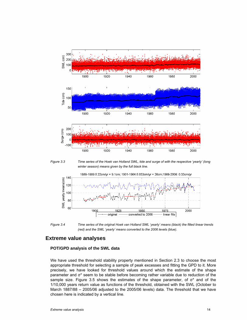
Yearly means of SWL and tide generally show trends and/or jumps due to sea level variations caused by global warming, dredging, coastal works and/or morphological changes. Figure 3.3 shows the time series of the Hoek van Holland SWL, tide and surge data from the 1887/88-2005/06 seasons and the corresponding ‘yearly’ (long winter season) means. The figure shows that the data contain two jumps: one in 1990 and the other in 1965. The latter is probably due to an extension of the Rotterdam Harbour (Maasvlakte, http://en.wikipedia.org/wiki/Maasvlakte) and the reason for the former is unknown. There are further visible trends in the data.

In order to homogenise the data the trends and jumps were removed and the data corrected to the levels of 2005/06; see Figure 3.4. The corrections were applied to the SWL data and a new tidal time series was computed by removing the surge from the corrected SWLs. The extreme value analyses presented in the following sections were carried out on the data corrected to the 2005/66 levels.


Figure 3.3 Time series of the Hoek van Holland SWL, tide and surge of with the respective ‘yearly’ (long

winter season) means given by the full black line.

Figure 3.4 Time series of the original Hoek van Holland SWL ‘yearly’ means (black) the fitted linear trends

(red) and the SWL ‘yearly’ means converted to the 2006 levels (blue).

Extreme value analyses

POT/GPD analysis of the SWL data

We have used the threshold stability property mentioned in Section 2.3 to choose the most appropriate threshold for selecting a sample of peak excesses and fitting the GPD to it. More precisely, we have looked for threshold values around which the estimate of the shape parameter and σ* seem to be stable before becoming rather variable due to reduction of the sample size. Figure 3.5 shows the estimates of the shape parameter, of σ* and of the 1/10,000 years return value as functions of the threshold, obtained with the SWL (October to March 1887/88 – 2005/06 adjusted to the 2005/06 levels) data. The threshold that we have chosen here is indicated by a vertical line.


Figure 3.5 Variation of the estimates of ξ, σ* and 1/10,000 years SWL return values of the GPD model with

the threshold used to collect the SWL POT sample.

Figure 3.6 Return value plot of the GPD model fitted to the SWL data obtained with the ML method (solid

black line) and associated 95% confidence intervals (dashed black lines). The POT data are represented by the asterisks.


The return value plot of the corresponding GPD fit is shown in Figure 3.6 and the model parameter estimates are presented in Table 3.1 (2nd column).

The return value plot suggests that the GPD model is appropriate for the data. Noteworthy is the position of the highest peak in the data, which corresponds to the SWL reached in the tragic storm of 1 February 1953 (converted to the 2006 levels). According to the plot, the return period of this event is much longer than the 119-year period covered by the data.

As can be seen in Table 3.1 (2nd column, 4th line), the estimate of the shape parameter is close to zero, which suggests that the data have a type I tail.

POT/GPD AM/GEV POT/GPD+conv. AM/GEV+conv

Sample size 265 119 336 119 u or μ̂ (cm) 220 241

(236, 246) 93 119 (114, 124)

ξ̂ 0.01 (-0.13, 0.13)

0.02 (-0.13, 0.15)

0.02 (-0.11, 0.12)

-0.03 (-0.17, 0.09)

σ̂% or σ̂ (cm) 26 (22, 30)

26 (22, 30)

26 (22, 30)

28 (24, 33)

1/10,000 yr surge (cm) ─ ─ 377 (267, 576)

345 (245, 507)

1/10,000 yr SWL (cm) 486 (381, 686)

505 (380, 739)

497 (409, 673)

467 (410,779)

Table 3.1 Parameter estimates and associated 95% confidence intervals of the models fitted to the SWL and surge data.

AM/GEV analysis of the SWL data

Figure 3.7 shows the return value plot of the GEV fit to the ‘annual’ (long winter season) maxima of the SWL data. Table 3.1 (3rd column) gives the corresponding parameter estimates.

The return value estimates for the 1/100, 1/1,000 and 1/10,000 years are given in Figure 3.7. Comparing these with the estimates obtained with the GPD model (Figure 3.6), one can conclude that they are compatible and rather close. The estimates of the shape parameters are also rather similar (cf. Table 3.1), supporting the validity of both models. As was to be expected (due to the difference in sample sizes), the confidence intervals provided by the GEV model are wider than those of the GPD.


Figure 3.7 Return value plot of the GEV fitted to the SWL data obtained with the ML method (solid black

line) and associated 95% confidence intervals (dashed black lines). The AM data are represented by the asterisks.

Convolution of astronomical tides and peak surge heights

As in the POT/GPD analysis of the SWL data, we have used the threshold stability property to choose the most appropriate threshold for selecting a sample of surge peak excesses and fitting the GPD to it. Figure 3.8 shows the estimates of the shape parameter, of σ* and of the 1/10,000 return value as functions of the threshold obtained with the surge (October to March 1887/88 – 2005/06) data. The thresholds that we have chosen are marked by vertical lines. The return value plot of the corresponding GPD fit is presented in Figure 3.9, and the model parameter estimates in Table 3.1 (4th column).

Comparing the GPD fits of the surge and SWL data (Figure 3.6 and Figure 3.9), one can say that the fit of the surge data is a bit poorer. As before, the highest peak of the surge data corresponds to the 1953 storm, which is again associated with a return period longer than that spanned by the measurements.


Figure 3.8 Variation of the estimates of ξ, σ* and 1/10,000 years surge return values of the GPD model with

the threshold used to collect the surge POT sample.

Figure 3.9 Return value plot of the GPD fitted to the surge data obtained with the ML method (solid black

line) and associated 95% confidence intervals (dashed black lines). The POT data are represented by the asterisks.


Figure 3.10 Observed and empirical distribution of the high water data from 1887/88 until 2005/06 adjusted

to 2005/06.

Figure 3.11 Return value plot of the convolution of the astronomical tide and the POT/GPD surge levels

(solid black line) and associated 95% confidence intervals (dashed black lines). The corresponding SWL POT data are represented by the asterisks.


Figure 3.10 shows the empirical distribution of the tide data from 1887/88 until 2005/06 corrected to 2005/06 (cf. 3.2.3). Figure 3.11 shows the return value plot obtained from the convolution of the empirical distribution of the astronomical tide and the GPD fit just described. The fit seems appropriate and the return value estimates are compatible with those obtained in Approach 1.

Convolution of astronomical tide and AM surge heights

Figure 3.12 shows the return value plot of the GEV fit to the annual maxima of the surge data and the surge 1/100, 1/1,000 and 1/10,000 years return value estimates. Table 3.1 (last column) gives the corresponding parameter estimates. Comparing these with the estimates obtained with the GPD model (Figure 3.9), one can conclude that they are lower but compatible. From Table 3.1 (4th line) one can also see that the estimates of the shape parameter, although compatible with the other, are the lowest of all estimates.

Figure 3.12 Return value plot of the GEV fitted to the surge data obtained with the ML method (solid black

line) and associated 95% confidence intervals (dashed black line). The surge data AM are represented by the asterisks.

Figure 3.13 shows the return value plot obtained from the convolution of the empirical distribution of the astronomical tide and the GEV fit just described. The fit seems appropriate and the return value estimates are compatible with those obtained from the SWL data using the other models.


Figure 3.13 Return value plot of the convolution of the astronomical tide and the AM surge levels (solid black

line) and associated 95% confidence intervals (dashed black lines). The corresponding SWL AM data are represented by the asterisks.

Discussion In the previous subsection approaches 1. and 2. have been applied to the Hoek van Holland data to estimating extremes of SWLs. Figure 3.15 shows the return value plots of the various SWL estimates and associated 95% confidence intervals. The figure shows a striking agreement between the return value point estimates provided by the different methods.

The compatibility between the estimates can be further seen in the relative differences between the SWL return value estimates obtained from the different analyses; cf. Table 3.2. Differences between estimates are always less than 5%. Given the amplitude of the 95% confidence intervals associated with the estimates (cf. Table 3.3), these differences do not appear significant. It can thus be concluded that, given a large enough and reliable dataset, the estimates of return values from the different approaches and variants should be compatible.

From the amplitude of the 95% confidence intervals in relation to the associated point estimate, given as a percentage in Table 3.3, the following conclusions can be drawn:

o The wider confidence intervals are those for estimates using the AM/GEV model. This is to be expected and may be even noticeable with datasets smaller than the one considered here.


o The use of Approach 2. does not result in smaller confidence intervals. This can be explained from the fact that the uncertainty in the estimates is due to the rare extreme events and not the well determined tide.

o As expected, the relative amplitude of the confidence intervals increases with the return period. This sets limitations to the actual use in practice of the ‘more extreme’ return value estimates computed from a dataset with a given length.

Figure 3.14 SWL return value plot constructed with the results from all the analyses, including 95%

confidence bands as dashed lines. The SWL POT data are represented by the asterisks.

Return period Convolution Residual POT/GPD

SWL AM/GPD

Convolution Residual AM/GPD

0.90 1.09 -0.21 1.54 2.36 -1.85

1/100 year 1/1,000 years

1/10,000 years 2.25 3.85 -4.08 Table 3.2 Relative differences between the SWL return values estimates obtained from the different

analyses and those of the POT/GPD analysis of the SWL. The values are percentages of the POT/GPD SWL return value point estimates.

For the return periods above 10 years, the return value estimates of the convolution are equal to those of the associated surge analysis plus a constant. Both in the POT and GPD models of Approach 2. this constant is 121 cm. The average of the high tide data for the period October to March 1887/88 – 2005/06 is 115 cm, and the maximum is 163 cm. The Mean High Water Spring at this site is 136 cm. This indicates that adding the Highest Astronomical Tide to the water levels associated with the extreme weather conditions of Approach 3. is a rather conservative procedure. A value between Mean High Water and Mean High Water Spring should be used, the mean high water spring being a slightly conservative value.

Return period SWL (cm) rel. amp. of c.i. (%) SWL 1/100 years 362 (329, 402) 20


POT/GPD 1/1,000 years 1/10,000 years

423 (358, 524) 486 (381, 686)

39 63

SWL AM/GEV

1/100 years 1/1,000 years

1/10,000 years

365 (329, 409) 433 (359, 547) 505 (380, 739)

22 43 71

Convolution Residual POT/GPD


1/10,000 years

365 (339, 409) 430 (378, 526) 497 (409, 673)

19 34 53

Convolution Residual AM/GEV


1/10,000 years

361 (341, 427) 416 (379, 576) 467 (410, 779)

24 47 79

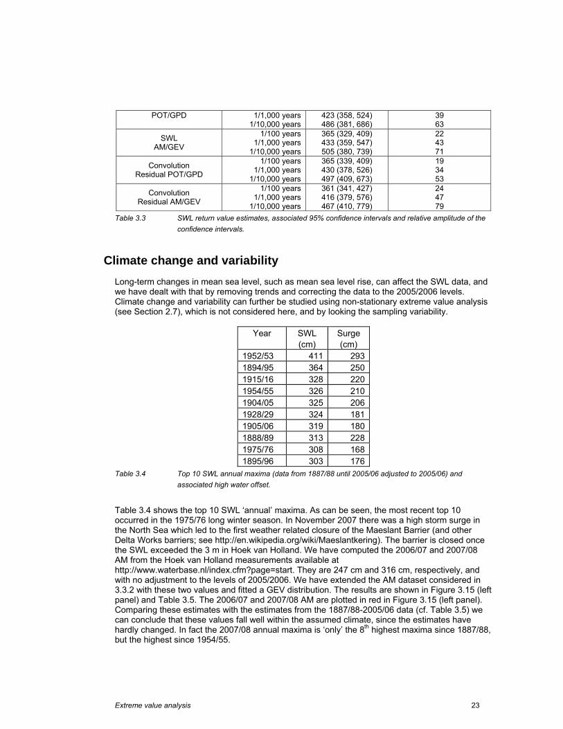
Table 3.3 SWL return value estimates, associated 95% confidence intervals and relative amplitude of the confidence intervals.

Climate change and variability Long-term changes in mean sea level, such as mean sea level rise, can affect the SWL data, and we have dealt with that by removing trends and correcting the data to the 2005/2006 levels. Climate change and variability can further be studied using non-stationary extreme value analysis (see Section 2.7), which is not considered here, and by looking the sampling variability.

Year SWL (cm)

Surge (cm)

1952/53 411 2931894/95 364 2501915/16 328 2201954/55 326 2101904/05 325 2061928/29 324 1811905/06 319 1801888/89 313 2281975/76 308 1681895/96 303 176

Table 3.4 Top 10 SWL annual maxima (data from 1887/88 until 2005/06 adjusted to 2005/06) and associated high water offset.

Table 3.4 shows the top 10 SWL ‘annual’ maxima. As can be seen, the most recent top 10 occurred in the 1975/76 long winter season. In November 2007 there was a high storm surge in the North Sea which led to the first weather related closure of the Maeslant Barrier (and other Delta Works barriers; see http://en.wikipedia.org/wiki/Maeslantkering). The barrier is closed once the SWL exceeded the 3 m in Hoek van Holland. We have computed the 2006/07 and 2007/08 AM from the Hoek van Holland measurements available at http://www.waterbase.nl/index.cfm?page=start. They are 247 cm and 316 cm, respectively, and with no adjustment to the levels of 2005/2006. We have extended the AM dataset considered in 3.3.2 with these two values and fitted a GEV distribution. The results are shown in Figure 3.15 (left panel) and Table 3.5. The 2006/07 and 2007/08 AM are plotted in red in Figure 3.15 (left panel). Comparing these estimates with the estimates from the 1887/88-2005/06 data (cf. Table 3.5) we can conclude that these values fall well within the assumed climate, since the estimates have hardly changed. In fact the 2007/08 annual maxima is ‘only’ the 8th highest maxima since 1887/88, but the highest since 1954/55.


We have also studied the effect of only considering the last 30 years of data in the estimates. Figure 3.15 (right panel) and Table 3.5 show the GEV estimates computed from the 1978/79-2005/06 AM data. The results show that although the confidence interval of the estimates intersect the estimates based on the whole dataset, the 1/10,000 SWL return value estimate is in this case about 1 metre less than that considering the whole data.

Figure 3.15 Return value plots of the GEV fitted to the SWL AM data obtained with the ML method (solid black line) and associated adjusted bootstrap 95% confidence intervals (dashed black lines). The AM data are represented by the asterisks. Left: Data from 1887/88-2007/08. Right: Data from 1978/79-2005/06.

1887/88-2005/06 1887/88-2007/08 1978/79-2005/06

Sample size 119 121 30 μ̂ (cm) 241

(236, 246) 241

(236, 246) 237

(228, 245)

ξ̂ 0.02 (-0.13, 0.15)

0.02 (-0.11, 0.15)

-0.02 (-0.37, 0.18)

σ̂ (cm) 26 (22, 30)

26 (22, 30)

21 (15, 28)

1/10,000 yr SWL (cm) 505 (380, 739)

507 (387, 712)

409 (304, 683)

Table 3.5 Parameter estimates and associated 95% confidence intervals of GEV models fitted to different periods SWL AM data.


Software packages

In the last decade or so, there has been an increased use of the extreme value methodology and an associated increased offer of software packages to perform extreme value analysis (see e.g. Stephenson and Gilleland, 2006). Many of the available packages target financial rather than environmental data. Without pretending to cover all that is available, Table 4.1 gives an overview of available extreme value analysis software packages directly suitable for the analysis of SWL data. Some have command line (routine) and/or Graphical User Interfaces (GUI). GUIs make packages very easy to use, but when not accompanied by command line / routine options they provide little flexibility to more experienced users. Package name and reference Programming

language Avail. Interface

EVIM http://www.bilkent.edu.tr/%7Efaruk/evim.htm

MATLAB free software

command line

EXTREMES http://mistis.inrialpes.fr/software/EXTREMES/accueil.html

C++ with a MATLAB GUI

free software

GUI

extRemes http://www.isse.ucar.edu/extremevalues/evtk.html Uses ismev

R free software

command line and GUI

ismev http://cran.r-project.org/web/packages/ismev/index.html (The R routines are based on the S-Plus (http://www.insightful.com/products/splus/) routines of Coles, 2001)

S-Plus and R free software

command line

ORCA http://www.wldelft.nl/soft/chess/orca/index.html

MATLAB commercial command line and GUI

Statistics of Extremes http://lstat.kuleuven.be/Wiley/index.html

S-Plus and FORTRAN

free software

command line

WAFO http://www.maths.lth.se/matstat/wafo/about.html

MATLAB free software

command line

Xtremes http://www.xtremes.de/xtremes/

Pascal commercial GUI

Table 4.1 Software packages available for EVA. Please note that web addresses may be liable to change. The analyses presented here were carried out using the MATLAB tool ORCA (“metOcean data tRansformation, Classification and Analysis tool”).


Recommendations

When carrying out an extreme value analysis of SWL or surge data we suggest that the following steps be followed: 1. The selection of the samples of SWL POT and/or AM, paying attention to declustering, so

that the data can be considered independent. 2. The selection of an extreme value distribution as a statistical model for the data produced

in the first step. According to theory the generalized Pareto distribution (GPD) should be selected when the sample is collected by means of the POT method, while in the case of the AM method a generalized extreme value (GEV) distribution should be chosen.

3. The selection of a method to estimate the unknown parameters of the distribution chosen in Step 2. Often the ML method is the most convenient and efficient.

4. When doing a POT/GPD analysis always produce threshold plots to guide the threshold choice.

5. On the basis of the estimated parameters (and thus the estimated distribution) the extreme values corresponding to one or more prescribed return period(s) can be estimated.

6. The selection of a method to quantify the uncertainty in the estimates of the distribution’s parameters and in the associated return values. The uncertainty in the parameters and return values is usually quantified by a confidence interval of some significance level (here 95%). Adjusted bootstrap confidence intervals are considered optimal.

Furthermore, we have the following recommendations:

o Before carrying out an extreme value analysis, a rigorous data quality analysis should always be carried out and eventual sea level trends removed.

o When the availability of data is limited, give preference to a POT/GPD analysis instead of AM/GEV analysis. Doing both would help as diagnostics. Nevertheless, several years (typically more than three) of good quality data are required so that the method considered here can be reliably used for estimation of extremes. There are three reasons for this:

1 In some cases with limited data (even with more than three years) fits to the extreme value distributions cannot be obtained due to limitations of the estimation methods.

2 Using only a few years of data can lead to bias due to longer term variations in the storm climate (consider the differences obtained were when considering 121 and 30 year periods).

3 Even if return value estimates can be obtained the confidence intervals will be very wide and of little value.

o The POT/GPD approach is generally preferable to the AM/GEV approach since the estimates of the latter have greater variability, even with long datasets.

o Approach 2. does not seem to be superior, in terms of reduction of uncertainty of estimates, to Approach 1. It is therefore preferable to use Approach 1. since this is simpler and/or does not require the determination of the tidal signal. In the case of the POT/GPD approach, this of course assumes that the threshold has been taken high enough so as to exclude peaks with no surge component.

o The choice of the offset to be used in Approach 2. should take into consideration the characteristics of the basin under study. For the North Sea, the basin of the example


used here, the instantaneous offset between the astronomical tide and the SWL should not be used since the two may be correlated. For other basins, such as for instance the Mediterranean Sea, where water depths are rather high and the wind set-up less important, the instantaneous offset can in principle be used. It can also be used when the basin is shallow but the tidal is relatively small.

o In Approach 3., the tidal level that should be added to the water level associated with extreme weather conditions should be somewhere between Mean High Waters and Mean High Water Spring.


References Caires, S., 2007: Extreme wave statistics. Confidence Intervals. WL | Delft Hydraulics Report H4803.30. Coles, S., 2001: An Introduction to the Statistical Modelling of Extreme Values. Springer Texts in Statistics,

Springer-Verlag: London. Coles, S., and E. Simiu, 2003: Estimating uncertainty in the extreme value analysis of data generated by a

hurricane simulation model. J. Eng. Mech., 129 (11), 1288-1294. Davison, A.C., and R.L. Smith, 1990: Models for exceedances over high thresholds (with discussion). J. Roy.

Stat. Soc., 52B, 393–442. De Vries, H., M. Breton, T. Demulder, J. Ozer, R. Proctor, K. Ruddick, J.C. Salomon and A. Voorrips, 1995: A

comparison of 2D storm-surge models applied to three shallow European seas. Environmental Software, 10(1), 23-42.

Dillingh, D., L. de Haan, R. Helmers, G.P. Können and J. van Malde, 1993: De basispeilen langs de Nederlandse kust; statistisch onderzoek (In Dutch). Rijkswaterstaat, Dienst Getijdenwateren /RIKZ, Report DGW-93.023.

Dixon, M.J. and J.A. Tawn, 1994: Extreme Sea-Levels at the UK A-Class Sites: Site-by-Site Analyses. Proudman Oceanographic Laboratory, Internal Document No. 65, 229 p.

Dixon, M. J., J.A. Tawn and J.M. Vassie, 1998: Spatial modelling of extreme sea levels. Environmetrics, 9, 283–301.

Efron, B. and Tibshirani, R.J., 1993: An Introduction to the Bootstrap. Monographs on Statistics & Applied Probability 57, Chapman and Hall/CRC, 436p.

Ferguson, T.S., 1996: A Course in Large Sample Theory, Chapman and Hall, New York. Ferreira, J.A., and C. Guedes Soares, 1998: An application of the peaks over threshold method to predict

extremes of significant wave height. J. Offshore Mech. Arct. Eng., 120, 165–176. Horsburgh, K.J. and C. Wilson, 2007: Tide-surge interaction and its role in the distribution of surge residuals

in the North Sea. J. Geophysical Res. Oceans, 112, C08003, doi:10.1029/2006JC004033 Hosking, J.R.M. and J.R. Wallis, 1987: Parameter and quantile estimation for the Generalized Pareto

Distribution. Technometrics, 29, 339–349. Hosking, J.R.M., J.R. Wallis, and E.F. Wood, 1985: Estimation of the generalized extreme-value distribution

by the method of probability-weighted moments. Technometrics, 27, 251-261. Leadbetter, M.R., G. Lindgren, and H. Rootzen, 1983: Extremes and related properties of random sequences

and series. Springer, New York. Pickands, J., 1971: The two-dimensional Poisson process and extremal processes. Journal of Applied

Probability, 8, 745-756. Pickands, J., 1975: Statistical inference using extreme order statistics. Annals of Statistics, 3, 119-131. Tajvidi, N., 2003: Confidence Intervals and Accuracy Estimation for heavy-tailed Generalized Pareto

Distributions. Extremes, 6, 111-123. WMO, 1998: Guide to Wave Analysis and Forecasting. WMO-N0. 702, 2nd edition, Geneva, Switzerland, 159

p., http://www.wmo.int/pages/prog/amp/mmop/documents/WMO%20No%20702/WMO702.pdf.


Glossary AM Annual maxima GEV Generalized extreme value distribution GPD Generalized Pareto distribution ML Maximum likelihood POT Peaks-over-threshold PWM Probability weighted moments SWL Still water level

Documents

EXTREME VALUE ANALYSIS: STILL WATER LEVEL