CLIMATE RESEARCHClim Res

Vol. 65: 87–105, 2015doi: 10.3354/cr01322

Published September 28

1. INTRODUCTION

The most widely used tools available for estimatingfuture crop yield responses to climate change areprocess-based crop models, and these are already

ap plied extensively in different parts of the world(Rosenzweig et al. 2013, Challinor et al. 2014b). Models have been constructed using a variety of ap -proaches for structuring and parameterising the basicprocesses influencing crop development and growth

© Inter-Research 2015 · www.int-res.com*Corresponding author: nina.pirttioja@ymparisto.fi

Temperature and precipitation effects on wheatyield across a European transect: a crop model

ensemble analysis using impact response surfaces

N. Pirttioja1,*, T. R. Carter1, S. Fronzek1, M. Bindi2, H. Hoffmann3, T. Palosuo4, M. Ruiz-Ramos5, F. Tao4, M. Trnka6,7, M. Acutis8, S. Asseng9, P. Baranowski10,

B. Basso11, P. Bodin12, S. Buis13, D. Cammarano14, P. Deligios15, M.-F. Destain16,B. Dumont16, F. Ewert3, R. Ferrise2, L. François16, T. Gaiser3, P. Hlavinka6,7, I. Jacquemin16,

K. C. Kersebaum17, C. Kollas17, J. Krzyszczak10, I. J. Lorite18, J. Minet16, M. I. Minguez5,M. Montesino19, M. Moriondo20, C. Müller21, C. Nendel17, I. Öztürk22, A. Perego8,

A. Rodríguez5, A. C. Ruane23,24, F. Ruget13, M. Sanna8, M. A. Semenov25, C. Slawinski10,P. Stratonovitch25, I. Supit26, K. Waha21,27, E. Wang28, L. Wu29, Z. Zhao28,30, R. P. Rötter4

1Finnish Environment Institute (SYKE), 00251 Helsinki, Finland2−30See title page of the Supplement at www.int-res.com/articles/suppl/c065p087_supp.pdf for full list of author addresses

ABSTRACT: This study explored the utility of the impact response surface (IRS) approach forinvestigating model ensemble crop yield responses under a large range of changes in climate.IRSs of spring and winter wheat Triticum aestivum yields were constructed from a 26-memberensemble of process-based crop simulation models for sites in Finland, Germany and Spain acrossa latitudinal transect. The sensitivity of modelled yield to systematic increments of changes in tem-perature (−2 to +9°C) and precipitation (−50 to +50%) was tested by modifying values of baseline(1981 to 2010) daily weather, with CO2 concentration fixed at 360 ppm. The IRS approach offersan effective method of portraying model behaviour under changing climate as well as advantagesfor analysing, comparing and presenting results from multi-model ensemble simulations. Thoughindividual model behaviour occasionally departed markedly from the average, ensemble medianresponses across sites and crop varieties indicated that yields decline with higher temperaturesand decreased precipitation and increase with higher precipitation. Across the uncertainty rangesdefined for the IRSs, yields were more sensitive to temperature than precipitation changes at theFinnish site while sensitivities were mixed at the German and Spanish sites. Precipitation effectsdiminished under higher temperature changes. While the bivariate and multi-model characteris-tics of the analysis impose some limits to interpretation, the IRS approach nonetheless providesadditional insights into sensitivities to inter-model and inter-annual variability. Taken together,these sensitivities may help to pinpoint processes such as heat stress, vernalisation or droughteffects requiring refinement in future model development.

KEY WORDS: Climate · Crop model · Impact response surface · IRS · Sensitivity analysis · Wheat ·Yield

Resale or republication not permitted without written consent of the publisher

Contribution to CR Special 31 'Modelling climate change impacts for food security' FREEREE ACCESSCCESS

Clim Res 65: 87–105, 2015

(Asseng et al. 2013). Such differences be tween modelapproaches introduce important sources of un cer -tainty into crop yield estimates, even for present-dayconditions (White et al. 2011). Model results are alsoclosely related to the quality of field observations andexperiments available for model calibration and test-ing (e.g. Craufurd et al. 2013) as well as the cali -bration methods themselves (Angulo et al. 2013).Moreover, there are numerous model shortcomingsin representing physiological processes that are stillpoorly understood (Rötter et al. 2011). These includecrop responses to stresses such as high temperature,drought, waterlogging, nutrient limitation, pests anddiseases, stomatal control on plant photosynthesis andtranspiration under changing atmospheric carbon di -oxide concentrations, and impacts of surface ozone(Porter et al. 2014).

Following early model comparison exercises (e.g.Porter 1993, Jamieson et al. 1998), and successive at-tempts by the Intergovernmental Panel on ClimateChange (IPCC) to assess climate change impacts oncrops across diverse models, regions, scenarios andassumptions (Gitay et al. 2001, Easterling et al. 2007,Porter et al. 2014), there has been a resurgence of in-terest in and establishment of dedicated research pro-grammes on model inter-comparison and im prove -ment (e.g. Palosuo et al. 2011, Rosenzweig et al. 2013,Challinor et al. 2014a). There have also been calls formore systematic modelling exercises for evaluatingthe suitability of crop model application under pro-jected climates, particularly climatic conditions thatlie beyond the ‘quantifiable uncertainty’ range of con-ventional local application (e.g. Rötter 2014). Of thefew systematic sensitivity studies that have been con-ducted, most focus on changes in average (mean ormedian) yields (e.g. Børgesen & Olesen 2011, Assenget al. 2013, Rosenzweig et al. 2014), whereas an addi-tional key consideration for farmers is the reliability ofthe harvest from year to year, which is addressed inonly a few studies (Luo et al. 2007, Challinor et al.2010, Iizumi et al. 2011, Asseng et al. 2014).

This paper presents an examination of the mod-elled sensitivity of winter and spring wheat Triticumaestivum yield response to systematic changes intemperature and precipitation, the 2 variables mostcommonly analysed in climate impact assessments. Itapplies a common impact response surface (IRS)approach for a large ensemble of process-basedwheat models run across a 3-site European transect.IRSs depict the response of an impact variable tochanges in 2 explanatory variables as a plotted sur-face. Other aspects that would need to be taken intoaccount if making projections of yield impacts under

climate change, such as the effect of increasingatmospheric CO2 concentration, are deliberately notincluded in the analysis. IRSs have been applied inprevious sensitivity studies of climate change im -pacts on permafrost (Fronzek et al. 2011), hydrology(Hanasaki et al. 2007, Wetterhall et al. 2011) and cropyield (Luo et al. 2007, Børgesen & Olesen 2011,Ruane et al. 2014). The approach was found to beeffective for the visualisation and rapid evaluation ofmodel sensitivities across a wide range of combina-tions of climate changes that are not specific to indi-vidual projections from climate models. Further, incombination with projections of climate variablesrepresented probabilistically, the approach can beapplied to estimate the likelihood of exceeding agiven impact threshold, such as a critical level ofyield (Børgesen & Olesen 2011).

Previous studies were based on individual modelsor emulators, whereas this is the first to apply IRSmethods across a large ensemble of models. Themain objective of the study was to demonstrate thecapabilities and limitations of the IRS approach forinvestigating model ensemble crop yield responsesunder a large range of foreseeable changes in cli-mate. The study’s specific aims, for the 2 crop vari-eties at each site, were (1) to explore the sensitivitiesof modelled yields to changes in temperature andprecipitation, (2) to quantify differences in averageyield responses to altered climate across models, and(3) to examine multi-model responses of inter-annualyield variability and reliability under altered climate.

2. MATERIALS AND METHODS

2.1. Crop models

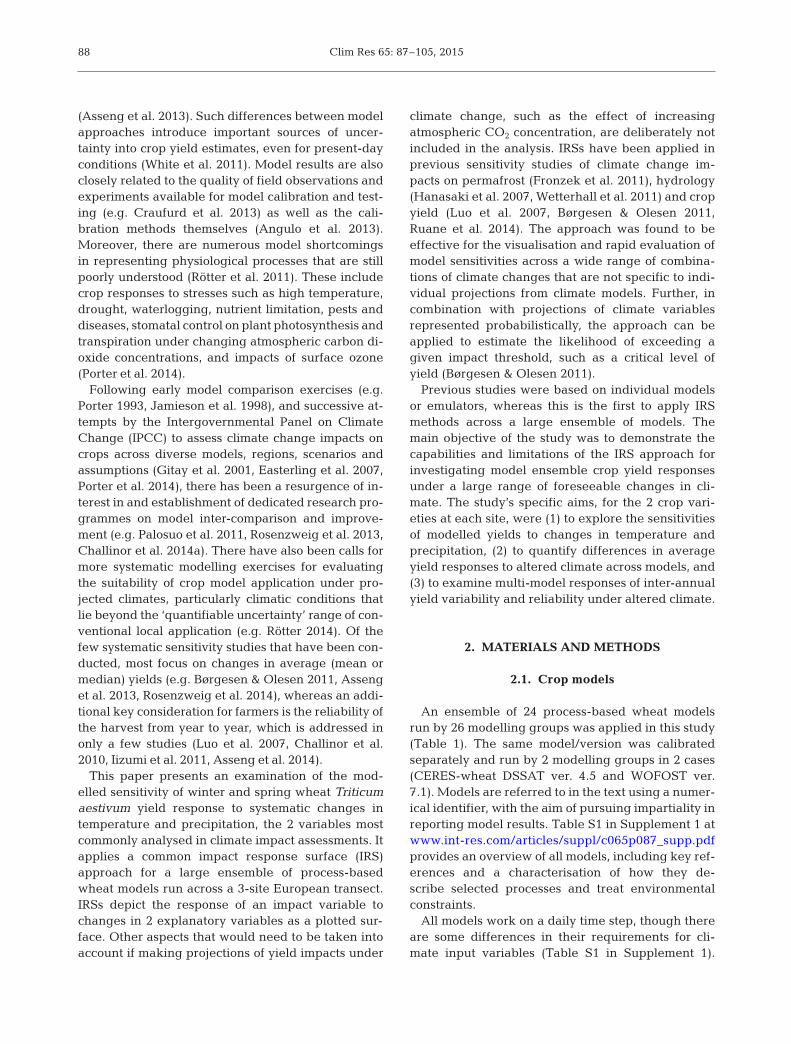
An ensemble of 24 process-based wheat modelsrun by 26 modelling groups was applied in this study(Table 1). The same model/version was calibratedseparately and run by 2 modelling groups in 2 cases(CERES-wheat DSSAT ver. 4.5 and WOFOST ver.7.1). Models are referred to in the text using a numer-ical identifier, with the aim of pursuing impartiality inreporting model results. Table S1 in Supplement 1 atwww. int-res. com/ articles/ suppl/ c065 p087 _ supp. pdfprovides an overview of all models, including key ref-erences and a characterisation of how they de -scribe selected processes and treat environmentalconstraints.

All models work on a daily time step, though thereare some differences in their requirements for cli-mate input variables (Table S1 in Supplement 1).

88

Pirttioja et al.: Impact response surfaces of wheat yield 89

Most models were developed for the field scale,while a few (i.e. CARAIB, LPJmL, LPJ-GUESS andMCWLA) have been developed for regional assess-ment. Models differ considerably in the way theytreat factors that define, limit or reduce growth (vanIttersum & Rabbinge 1997, van Ittersum et al. 2003,Wu & Kersebaum 2008), which is reflected in con-trasting structure, model parameters and associatedinput data requirements.

2.2. Study sites and key data requirements

2.2.1. Criteria for the selection of study sites

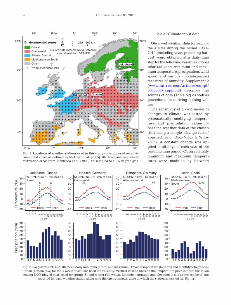
The models were applied using data from 4 studysites representing contrasting environmental zones(Boreal, Atlantic Central, Continental and Mediter-ranean South) for wheat production in Europe (ourFig. 1; Metzger et al. 2005). The study sites wereselected according to multiple criteria. A primary ob -jective was to offer a representative north-southcross-section (transect) of current agro-climatic con-ditions for wheat cultivation areas in Europe. Sec-

ondly, the sites should capture the contrast in rain-fed yield potential between favourable conditions inCentral Europe and growth conditions at the north-ern margins (limited by temperature) and southernmargins (limited by precipitation). Thirdly, optionsfor adapting to anticipated future climate should in -clude the possibility to substitute winter wheat typeswith spring wheat types and vice versa. Finally, cropdata should be available for site-specific calibrationof the crop models, while daily weather data for run-ning the models were required for the baselineperiod of 1981 to 2010 at each site.

To keep the number of simulations manageable,one site was chosen in each of northern, central andsouthern Europe for each crop variety. Jokioinen inFinland was chosen for northern Europe and Lleida inSpain for southern Europe. Since sufficient cali bra -tion data for modern cultivars that would cover bothwinter wheat and spring wheat at a single site in cen-tral Europe were not available, 2 sites in Germanywere chosen: Dikopshof, located in the west, for win-ter wheat and Nossen in the east, for spring wheat.The principal characteristics of the 4 sites and theiragro-climatic conditions are summarised in Fig. 2.

ID Model Contact person(s) Web documentation

1 AFRCWHEAT2 Montesino/Porter −2 APSIM-Nwheat 1.55 Cammarano/Asseng www.apsim.info3 APSIM-Wheat (modified) 7.5 Wang www.apsim.info4 AquaCrop 4.0 Lorite www.fao.org/nr/water/aquacrop.html5 ARMOSA13.04 Perego/Sanna/Acutis −6 CARAIB Crop Minet/Jacquemin/François www.umccb.ulg.ac.be/Sci/m_car_e.html7 CERES-wheat DSSAT v.4.5 Ruiz-Ramos http://dssat.net8 CERES-wheat DSSAT v.4.5 Deligios http://dssat.net9 CERES-wheat DSSAT v.4.6 Trnka/Hlavinka http://dssat.net10 CropSyst 3.02 Moriondo/Ferrise/Bindi modeling.bsyse.wsu.edu/CS_Suite_4/CropSyst11 DNDC 9.5 Baranowski/Slawinski www.dndc.sr.unh.edu12 Fasset 2.5 Öztürk/Olesen www.fasset.dk13 HERMES V 4.26 Kersebaum/Kollas www.zalf.de/en/forschung/institute/lsa/ forschung/

http://oekomod/ hermes14 LINTUL-4 v6 Supit/Wolf http://models.pps.wur.nl/models15 LPJ-GUESS Bodin/Olin www.nateko.lu.se/lpj-guess16 LPJmL Müller www.pik-potsdam.de/research/projects/lpjml17 MCWLA-Wheat 2.0 Tao −18 MONICA 1.2.5 Nendel http://monica.agrosystem-models.com/en19 SALUS Basso http://salusmodel.psm.msu.edu/20 SIMPLACE<Lintul2, Slim> Hoffmann/Gaiser/Ewert www.simplace.net/, http://models.pps.wur.nl/models21 Sirius Semenov/Stratonovitch www.rothamsted.ac.uk/mas-models/sirius.php22 SiriusQuality 2.0 Ferrise/Bindi www1.clermont.inra.fr/siriusquality23 SPACSYS 5.0 Wu −24 STICS V6.9 Dumont/Ruget/Buis www6.paca.inra.fr/stics25 WOFOST 7.1 Palosuo/Rötter www.wofost.wur.nl26 WOFOST 7.1 Krzyszczak/Slawinski www.wofost.wur.nl

Table 1. List of wheat models applied in the present study. ID is a model identification number used in the text. Duplicate entries indicate models for which several groups provided results

Clim Res 65: 87–105, 2015

2.2.2. Climate input data

Observed weather data for each ofthe 4 sites during the period 1980−2010 (including years preceding har-vest) were obtained at a daily timestep for the following variables: globalsolar radiation, minimum and maxi-mumtemperature,precipitation,windspeed and various (model- specific)measures of humidity. Supplement 2(www. int-res. com/ articles/ suppl/c065 p087 _ supp. pdf) de scribes thesources of data (Table S2) as well asprocedures for deriving missing val-ues.

The sensitivity of a crop model tochanges in climate was tested bysystematically modifying tempera-ture and precipitation values ofbaseline weather data at the chosensites using a simple ‘change factor’approach (e.g. Diaz-Nieto & Wilby2005). A constant change was ap -plied to all days of each year of thebaseline time period. Observed dailyminimum and maximum tempera-tures were modified by be tween

90

30°

30°

20°

20°

10°E

10°E

0°

0°

10°W

10°W20°

70°N 70°N

60° 60°

50° 50°

40° 40°

Environmental zones

Boreal

Continental

Atlantic Central

Mediterranean South

Other

Wheat cultivation area

0 500250 km

Jokioinen

NossenDikopshof

Lleida

Co-ordinate system: World Robinsoncentral meridian: 30°0’0”E

Fig. 1. Locations of weather stations used in this study superimposed on envi-ronmental zones as defined by Metzger et al. (2005). Black squares are wheatcultivation areas from Monfreda et al. (2008), re-sampled to a 0.5 degree grid

Jokioinen, Finland

DOY

Tem

per

atur

e (°

C)

1 31 61 91 121

151

181

211

241

271

301

331

361

-20

-10

0

10

20

30

40

Tmax Tmin

S W

60.81°N, 23.50°E, 104 m a.s.l.Boreal

Nossen, Germany

DOY

1 31 61 91 121

151

181

211

241

271

301

331

361

-20

-10

0

10

20

30

40

Tmax Tmin

S

51.06°N, 13.27°E, 255 m a.s.l.Continental

Dikopshof, Germany

DOY

1 31 61 91 121

151

181

211

241

271

301

331

361

-20

-10

0

10

20

30

40

Tmax Tmin

W

50.81°N, 6.95°E , 60 m a.s.l. Atlantic Central

Lleida, Spain

DOY

1 31 61 91 121

151

181

211

241

271

301

331

361

-20

-10

0

10

20

30

40

Tmax Tmin

S/W

41.63°N, 0.60°E, 190 m a.s.l.MediterraneanSouth

Pre

cip

itatio

n (m

m)

0102030405060708090

J F M A M J J A S O N D 0102030405060708090

J F M A M J J A S O N D 0102030405060708090

J F M A M J J A S O N D 0102030405060708090

J F M A M J J A S O N D

Fig. 2. Long-term (1981−2010) mean daily minimum (Tmin) and maximum (Tmax) temperature (top row) and monthly total precip-itation (bottom row) for the 4 weather stations used in this study. Vertical dashed lines on the temperature plots indicate the meansowing DOY (day of year) used for spring (S) and winter (W) wheat. Latitude, longitude and elevation (a.s.l.: above sea level) are

reported for each weather station along with the environmental zone in which the station is located (cf. Fig. 1)

Pirttioja et al.: Impact response surfaces of wheat yield

−2°C and + 9°C at 1°C intervals and concurrently(preserving the baseline diurnal temperature range).Daily precipitation was adjusted between −50% and+50% at 10% intervals. The ranges were selected tobe large enough to encompass changes in regionalclimate change at the 4 sites by the mid-21st centuryrepresented in probabilistic projections (for mediumemissions; Harris et al. 2010) as well as in projectionsfrom an ensemble of general circulation models thatparticipated in the Coupled Model IntercomparisonProject phase 5 (IPCC 2013a). The increments of thechanges were chosen to be small enough to representpossible non-linearities in model responses to achanging climate, while at the same time ensuring amanageable number of combinations. Thus, eachyear of the baseline was modified according to 132different combinations of changed temperature andprecipitation and provided as input to the models.

For simplicity, all other variables were unchangedat their baseline values. Note that this procedureintroduced a discrepancy between models in the wayhumidity was treated. This is because in order tomaintain a constant level of relative humidity (RH) astemperature rises, vapour pressure (e) must also in -crease. Thus, by fixing e and RH at baseline values,the 7 models that required e as an input would haveover-estimated evapotranspiration under higher tem-peratures compared to those models requiring RH.The effect of this discrepancy was evaluated usingone of the models and then extrapolated to all 8 setsof runs affected. While yield declines were indeedgreater under conditions of extreme warming anddrying, the overall effect on the ensemble resultsreported below was minimal and the conclusions areunaffected.

2.2.3. Sowing date, soil and calibration data

For the Finnish site and the 2 sites in Germany, aspecific sowing date was determined for each year ofthe (30 yr) baseline period based on observations. Inthe absence of observed sowing dates for Spain, 1fixed sowing date (day of the year [DOY] 302), iden-tified on the basis of local expertise, was used for allyears and for both spring wheat and winter wheat.Following local practice, it was assumed that farmersat the Spanish site (Lleida) can use the same sowingdate for both crop varieties and would sow as early aspossible after the autumn rain, approximately at theend of October.

Additional data were made available for model cal-ibration. To avoid over-fitting, where possible, data

sets were used that had not previously been appliedin model calibration and/or were not fully docu-mented in published papers. Model users were pro-vided with phenological observations and yields fromeach location and for both crop varieties. Total above-ground biomass and average grain weights were alsoprovided for the Spanish site (Cartelle et al. 2006,Abeledo et al. 2008). As an alternative to the gener-alised soil type used for the model simulations (clayloam), modellers had the option to use information onthe actual soil of the site for calibration. In addition tothe sowing dates provided for the simulations, cali-bration data on management included sowing depthsas well as data of varying detail on fertilisation, irri-gation, tillage and residue management. Overall,calibration data on plant development in cludedobservations from between 5 and 29 seasons or treat-ments, depending on site and wheat variety (seeTable S2 in Supplement 2).

2.3. Modelling protocol

A sensitivity analysis was performed by runningthe models for the 30 baseline years and 132 pertur-bations to the baseline weather for spring and winterwheat at all study sites (3 sites per crop) resulting in23 760 simulated seasons per model. In the simulationset-up several common rules and limitations werespecified. This included applying baseline sowingdates for all temperature and precipitation perturba-tions and assuming a generalised soil type at all sites.Atmospheric CO2 concentration was kept constant at360 ppm, representing levels observed around 1995(IPCC 2013b, p. 1401), at the mid-point of the 1981 to2010 baseline period. The simulations were per-formed on a daily time step for water-limited yieldsas suming optimal nutrients. Simulations were con-ducted as a succession of independent growing sea-sons with the moisture content of the top soil set at75% of field capacity at the beginning of each season.

Model outputs were stored on a yearly resolution.For each simulation the flowering date (Zadoks stage65; Zadoks et al. 1974), date of physio logical maturity(Zadoks stage 91) and harvest date (model-specific)were stored as the day of the year (DOY). Harvestedyields were represented as grain dry matter (DM),while total above ground DM production and nitrogencontent of yield were also reported for the end of eachsimulation. Water use was stored as cumulative actualevapotranspiration (mm) from sowing to maturity.

For models that do not specify a latest date for harvest, simulations in some seasons may continue

91

Clim Res 65: 87–105, 2015

through to a maturity date in the year subsequentto the harvest year. This unrealistic outcome wasavoided by imposing a fixed maturity cut-off date,based on expert judgement, in the autumn of the har-vest year (DOY 258 for Finland and Spain and DOY274 for both German sites). If a simulation reported amaturity date that exceeded the harvest cut-off, theDM grain yield and grain nitrogen content were setto 0 (kg ha−1) and all other output variables were as -signed missing values. It was assumed that before acrop reached maturity it was not fit for harvest, sothat no DM yield was recorded. All modelling groupswere given the chance to review initial IRS plots ofthe results and to iterate by refining the calibration ofa model or correcting any errors, often themselvesreadily detectable from the IRS plots.

2.4. Construction and analysis of impact responsesurfaces

IRSs were constructed by interpolating the resultsof the sensitivity analysis of each model as contourlines with respect to changes in annual temperaturealong the x-axis and precipitation along the y-axis.The contour lines were plotted using the contour(Becker et al. 1988) and filled.contour (Cleveland1993) functions in the statistical software package Rver. 3.0.2 (R Core Team 2013). Individual IRSs werecreated for each model and combination of parame-ters (i.e. site, crop variety, harvest year).

In this paper we concentrated on analysing resultsof DM grain yields and their changes relative to thebaseline for the model ensemble. For summarisingaverage yield responses and their dispersion, weused 2 types of measures. Across different models inthe ensemble we used medians for average re -sponses, in line with earlier multi-model ensemblestudies (e.g. Asseng et al. 2013, and see our Section4.1), and the inter-quartile range (IQR; from the 25thto the 75th percentile) for the spread of responses.Over periods of time (in most cases, 30 yr) we usedmeans, though some results from individual years arealso shown. Inter-annual variability was treated in 2ways. The year-to-year ‘reliability’ of yields was rep-resented, for any individual model, as the percentageof years when DM grain yield (kg ha−1) exceeds agiven threshold level. Here, reliability is defined rel-ative to the 10th percentile of yields during the base-line period (i.e. the level of yield that was exceededin 9 yr out of 10). The threshold is defined only acrossthose years that have a non-zero yield for the base-line period. An alternative to focusing on reliability at

the low end of yield responses is to plot the coeffi-cient of variation (CV) across the 30 yr, which ac -counts for the full distribution of yield responses.Both measures of inter-annual variability were esti-mated for each 30 yr simulation period under all com-binations of temperature and precipitation changerelative to the baseline.

3. RESULTS

3.1. Baseline yields and standardisation of yieldresponses

3.1.1. Baseline yields

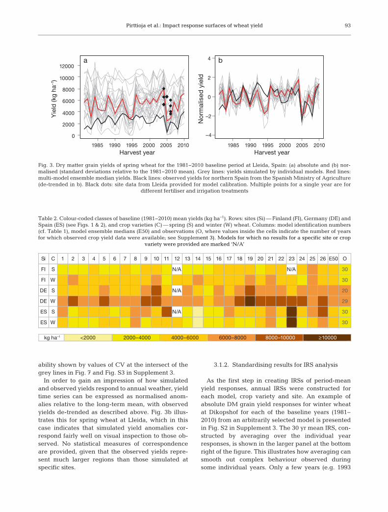
Examination of the general magnitude of modelledyields for the baseline period of 1981 to 2010 re -vealed large differences both between individualmodels as well as between simulated yields and ob -served aggregate regional yields, where these wereavailable (see Supplement 3 at www. int-res. com/ articles/ suppl/ c065 p087 _ supp. pdf). This is particu-larly true for Lleida, where the spread across modelsin simulated yields of both spring and winter wheatwas large, and the model ensemble median yield wasconsiderably higher than that observed. Fig. 3adepicts results for spring wheat at Lleida (for otherlocations and crop varieties see Fig. S1 in Supple-ment 3). The ensemble median of simulated yieldsexceeded those observed in most years and for bothvarieties at Jokioinen (Fig. S1a,b), whereas observedvs. modelled yields were much closer at the 2 Ger-man sites (Fig. S1c,d).

The levels of observed and modelled baseline(1981− 2010) mean yields are summarised in Table 2.Yields varied widely between models, ranging from1260 kg ha−1 (Model 14 for spring wheat in Spain) to10484 kg ha−1 (Model 19 for winter wheat in Ger-many), while the range of observed regional yieldswas 2556 to 7529 kg ha−1. The highest model esti-mates are up to 8 times greater than the lowest esti-mates for the same site and crop variety, with thehighest yields found at the German sites in both setsof observed statistics as well as for most models andfor the ensemble medians (Table 2). The inter-annualvariability of observed yields (adjusted to account forlong-term trends assumed to be unrelated toweather), as represented by the CV (not shown), waslowest in the 2 German regions, higher in Finland andsubstantially higher in northern Spain. These ob -served regional differences were consistent withmodelled between-site estimates of inter-annual vari-

92

Pirttioja et al.: Impact response surfaces of wheat yield

ability shown by values of CV at the intersect of thegrey lines in Fig. 7 and Fig. S3 in Supplement 3.

In order to gain an impression of how simulatedand observed yields respond to annual weather, yieldtime series can be expressed as normalised anom-alies relative to the long-term mean, with observedyields de-trended as described above. Fig. 3b illus-trates this for spring wheat at Lleida, which in thiscase indicates that simulated yield anomalies cor -respond fairly well on visual inspection to those ob -served. No statistical measures of correspondenceare provided, given that the observed yields repre-sent much larger regions than those simulated atspecific sites.

3.1.2. Standardising results for IRS analysis

As the first step in creating IRSs of period-meanyield responses, annual IRSs were constructed foreach model, crop variety and site. An example ofabsolute DM grain yield responses for winter wheatat Dikopshof for each of the baseline years (1981−2010) from an arbitrarily selected model is presentedin Fig. S2 in Supplement 3. The 30 yr mean IRS, con-structed by averaging over the individual yearresponses, is shown in the larger panel at the bottomright of the figure. This illustrates how averaging cansmooth out complex behaviour observed duringsome individual years. Only a few years (e.g. 1993

93

Si C 1 2 3 4 5 6 7 8 9 10 11 12 13 14 15 16 17 18 19 20 21 22 23 24 25 26 E50 O

FI S N/A N/A 30

FI W 30

DE S N/A 20

DE W 29

ES S N/A 30

ES W 30

kg ha–1 <2000 2000–4000 4000–6000 6000–8000 8000–10000 ≥10000

Table 2. Colour-coded classes of baseline (1981−2010) mean yields (kg ha−1). Rows: sites (Si) — Finland (FI), Germany (DE) andSpain (ES) (see Figs. 1 & 2), and crop varieties (C) — spring (S) and winter (W) wheat. Columns: model identification numbers(cf. Table 1), model ensemble medians (E50) and observations (O, where values inside the cells indicate the number of yearsfor which observed crop yield data were available; see Supplement 3). Models for which no results for a specific site or crop

variety were provided are marked ‘N/A’

Harvest year

Y

ield

(kg

ha–1)

1985 1990 1995 2000 2005 2010

0

2000

4000

6000

8000

10000

12000a

Harvest year

Nor

mal

ised

yie

ld

–4

–2

0

2

4 b

1985 1990 1995 2000 2005 2010

Fig. 3. Dry matter grain yields of spring wheat for the 1981−2010 baseline period at Lleida, Spain: (a) absolute and (b) nor-malised (standard deviations relative to the 1981−2010 mean). Grey lines: yields simulated by individual models. Red lines:multi-model ensemble median yields. Black lines: observed yields for northern Spain from the Spanish Ministry of Agriculture(de-trended in b). Black dots: site data from Lleida provided for model calibration. Multiple points for a single year are for

different fertiliser and irrigation treatments

Clim Res 65: 87–105, 2015

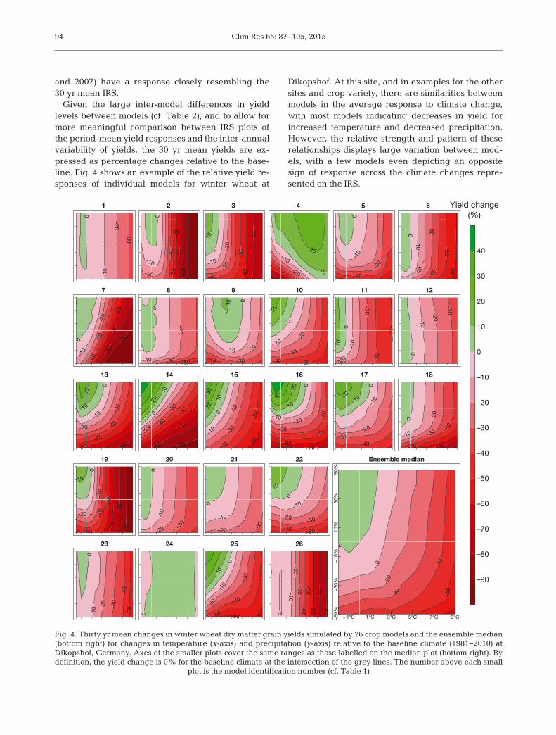
and 2007) have a response closely resembling the30 yr mean IRS.

Given the large inter-model differences in yieldlevels between models (cf. Table 2), and to allow formore meaningful comparison between IRS plots ofthe period-mean yield responses and the inter-annualvariability of yields, the 30 yr mean yields are ex-pressed as percentage changes relative to the base-line. Fig. 4 shows an example of the relative yield re-sponses of individual models for winter wheat at

Dikopshof. At this site, and in examples for the othersites and crop variety, there are similarities be tweenmodels in the average response to climate change,with most models indicating decreases in yield for increased temperature and decreased precipitation.However, the relative strength and pattern of theserelationships displays large variation be tween mod-els, with a few models even depicting an oppositesign of response across the climate changes repre-sented on the IRS.

94

–90

–80

–70

–60

–50

–40

–30

–20

–10

0

10

20

30

40

Yield change(%)

Ensemble median

–50

–40

–30

–20

–10

0

−1°C 1°C 3°C 5°C 7°C 9°C–50%

–30%

–10%

10%

30%

50%

1

–30

–20

–10

0

2

–80

–

70

–60

–

50

–40

–20

–10

0

3

–70

–60

–

50

–40

–30

–

20

–10

0

10

4

–20

–10

10

20

5

–40

–30

–10

0

6

–60

05–

–40

–

30

–20

–10 0

7

–90

–80

–

70

–60

–40

–

30

–20

–10

0

8

–50 –30

–20

–10

0

9

–40 –30

–20

–10

0

10

10

–50 –40 –30

–20

–10

0

20

11

–50

–40

–30

–20

–10

0

10

12

–30

–20

–10

0

13

–80 –60

–50

–40

–30

–20 –1

0

0

10

20

14

–90 –80

–70

–50

–40

–30

–20

0

10

20

15

–60

–

50

–40

–30

–

20

–10

0

10

20

30

16

–70 –60

–50

–40

–30 –20

–10

0

10

20

30

17

–40 –30

–20

–10

0

10 20

18

–70 –50 –4

0

–30 –

20

–10

0

19

–90

–

80

–70

–

60

–50

–40

–

30

–20

0

10

20

–30

–20

–10

0

21

–30

–20

–10

0

22

–50 –40 –30 –20

–10

0

10

23

–50

–

40

–30

–20

–10

0

24

0

25

–60 –50

–40

–30

–20

–10

0

10

26

–80 –70

–60 –50

–40 –30

–20 –10

0

Fig. 4. Thirty yr mean changes in winter wheat dry matter grain yields simulated by 26 crop models and the ensemble median(bottom right) for changes in temperature (x-axis) and precipitation (y-axis) relative to the baseline climate (1981−2010) atDikopshof, Germany. Axes of the smaller plots cover the same ranges as those labelled on the median plot (bottom right). Bydefinition, the yield change is 0% for the baseline climate at the intersection of the grey lines. The number above each small

plot is the model identification number (cf. Table 1)

Pirttioja et al.: Impact response surfaces of wheat yield

3.2. IRS analysis: multi-model 30 yr mean yieldresponses

3.2.1. Ensemble median changes

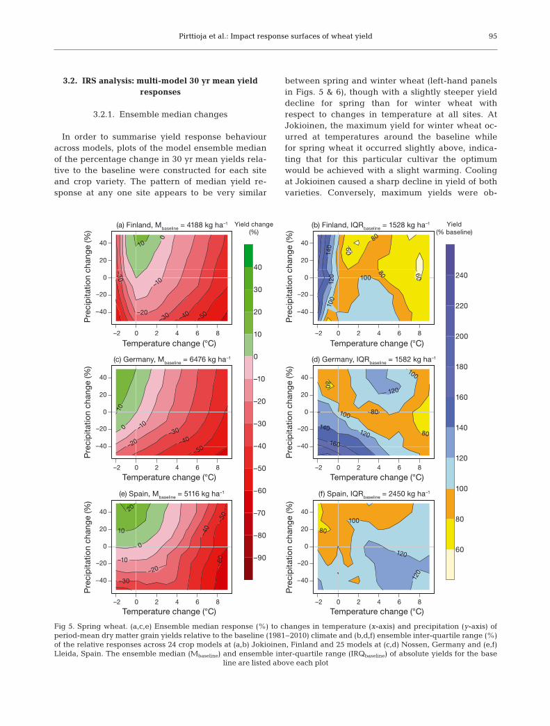
In order to summarise yield response behaviouracross models, plots of the model ensemble medianof the percentage change in 30 yr mean yields rela-tive to the baseline were constructed for each siteand crop variety. The pattern of median yield re -sponse at any one site appears to be very similar

be tween spring and winter wheat (left-hand panelsin Figs. 5 & 6), though with a slightly steeper yielddecline for spring than for winter wheat withrespect to changes in temperature at all sites. AtJoki oinen, the maximum yield for winter wheat oc -urred at temperatures around the baseline whilefor spring wheat it occurred slightly above, indica-ting that for this particular cultivar the optimumwould be achieved with a slight warming. Coolingat Jokioinen caused a sharp decline in yield of bothvarieties. Conversely, maximum yields were ob -

95

(a) Finland, Mbaseline = 4188 kg ha–1 (b) Finland, IQRbaseline = 1528 kg ha–1

(c) Germany, Mbaseline = 6476 kg ha–1

Temperature change (°C)

Temperature change (°C)

Temperature change (°C)

Temperature change (°C)

(d) Germany, IQRbaseline = 1582 kg ha–1

(e) Spain, Mbaseline = 5116 kg ha–1

Pre

cip

itatio

n ch

ange

(%)

Pre

cip

itatio

n ch

ange

(%)

Pre

cip

itatio

n ch

ange

(%)

(f) Spain, IQRbaseline = 2450 kg ha–1

–2 0 2 4 6 8

–40

–20

0

20

40

–50 –40

–30

–30 –20

–10

0

10

–90

–80

–70

–60

–50

–40

–30

–20

–10

0

10

20

30

40

–2 0 2 4 6 8

–40

–20

0

20

40 60

60

80

80

100

100

120

1

40

60

80

100

120

140

160

180

200

220

240

–2 0 2 4 6 8

–40

–20

0

20

40

Temperature change (°C) Temperature change (°C)

–50 –40 –30

–20

–10

0

10

–2 0 2 4 6 8

–40

–20

0

20

40 80

80

80

100

100

120

120

140

160

–2 0 2 4 6 8

–40

–20

0

20

40

Pre

cip

itatio

n ch

ange

(%)

Pre

cip

itatio

n ch

ange

(%)

Pre

cip

itatio

n ch

ange

(%)

–60

–

50

–40

–30 –20

–10

0

10

20

–2 0 2 4 6 8

–40

–20

0

20

40

80

100

120

120

Yield change(%)

Yield(% baseline)

Fig 5. Spring wheat. (a,c,e) Ensemble median response (%) to changes in temperature (x-axis) and precipitation (y-axis) of period-mean dry matter grain yields relative to the baseline (1981−2010) climate and (b,d,f) ensemble inter-quartile range (%)of the relative responses across 24 crop models at (a,b) Jokioinen, Finland and 25 models at (c,d) Nossen, Germany and (e,f)Lleida, Spain. The ensemble median (Mbaseline) and ensemble inter-quartile range (IRQbaseline) of absolute yields for the base

line are listed above each plot

Clim Res 65: 87–105, 201596

tained with cooling relative to the baseline at theGerman sites and at Lleida.

For combinations of temperature and precipitationchange across the uncertainty ranges defined for theIRS, temperature was the dominant constraint onmedian yield at all sites for warming above about5°C. Under conditions of less warming, precipitationhad an increasing influence across the transect fromnorth to south, with median yields most sensitive atLleida. Contour lines were nearly vertical in areas ofthe climate uncertainty space with increases in pre-cipitation at Jokioinen and at the German sites, inparticular for winter wheat, indicating that precipita-tion change had hardly any effect on yield in theseregions of the IRS.

3.2.2. Ensemble inter-model variability

In contrast to the similarities of median yield re -sponse to temperature and precipitation change be -tween crop varieties at each site and broadly acrosssites, there are marked differences in the inter-modelvariability of responses. Plots of the ensemble IQRde pict the spread in the 30 yr mean response tochanges in temperature and precipitation (right-hand panels, Figs. 5 & 6). The absolute IQR for thebase line (shown above each figure) is scaled to 100%at the origin of the plot for all models, and values ofIQR across the IRS are expressed as percentages ofthe baseline. For example, values for spring wheat atLleida are percentages of the baseline IQR of 2450 kg

(a) Finland, Mbaseline = 5155 kg ha–1 (b) Finland, IQRbaseline = 1277 kg ha–1

(c) Germany, Mbaseline = 7995 kg ha–1

Temperature change (°C)

Temperature change (°C)

Temperature change (°C)

Temperature change (°C)

(d) Germany, IQRbaseline = 1341 kg ha–1

(e) Spain, Mbaseline = 4005 kg ha–1

Pre

cip

itatio

n ch

ang

e (%

)P

reci

pita

tion

chan

ge

(%)

Pre

cip

itatio

n ch

ang

e (%

)

(f) Spain, IQRbaseline = 2165 kg ha–1

–2 0 2 4 6 8

–40

–20

0

20

40

–2 0 2 4 6 8

–40

–20

0

20

40

–2 0 2 4 6 8

–40

–20

0

20

40

Temperature change (°C) Temperature change (°C)

–2 0 2 4 6 8

–40

–20

0

20

40

–2 0 2 4 6 8

–40

–20

0

20

40

Pre

cip

itatio

n ch

ang

e (%

)P

reci

pita

tion

chan

ge

(%)

Pre

cip

itatio

n ch

ang

e (%

)

–2 0 2 4 6 8

–40

–20

0

20

40

Yield change(%)

Yield(% baseline)

–40

–30 –20

–10 0

100

120

120

140

140

160

180

–40 –30

–20 –10

100 120

120

140 160

160

180

180

200

200

220

–40 –30

–20 –10

0 10

20

30

60

80

80

100

100

–90

–80

–70

–60

–50

–40

–30

–20

–10

0

10

20

30

40

60

80

100

120

140

160

180

200

220

240

Fig. 6. As Fig. 5, but for winter wheat and for an ensemble of 26 crop models at (a,b) Jokioinen, Finland, (c,d) Dikopshof, Germany and (e,f) Lleida, Spain

Pirttioja et al.: Impact response surfaces of wheat yield

ha−1 (Fig. 5f). Note that variability across a wider dis-tribution of models (10th to 90th and 5th to 95th per-centiles) was also examined, with patterns found tobe broadly similar to the IQR patterns reported here.

The results showing the highest consistency be -tween sites or crop varieties are the increased IQRvalues for Jokioinen under cooling for both springand winter wheat (Figs. 5b & 6b, respectively). Theinter-model spread for spring wheat was lower thanthe baseline under most cases of warming, except fora slight increase for reduced precipitation combinedwith moderate warming (Fig. 5b). For winter wheatunder warming, there is some similarity between IQRpatterns for Jokioinen and Dikopshof, which in -creased under moderate to high levels of warmingand reduced precipitation (Fig. 6b,d), though modelspread was lowest under slightly warmer conditionsat Jokioinen but cooler conditions at Dikopshof.

The inter-model variability of spring wheat yields atNossen was lowest for combinations of temperatureand precipitation change between the wettest, coolestconditions and the warmest conditions, with lessagreement between modelled yields (higher IQR) formoderate warming and increased precipitation or fordrying combined with cooling or moderate warming(Fig. 5d).

The IQR broadly followed the median yield re -sponse for spring wheat at Lleida, with highest yieldscoinciding with the lowest inter-model variabilityand increasing spread as yields declined with highertemperature and reduced precipitation (compareFig. 5e and f). In contrast, for winter wheat at Lleida,the IQR was lower than the baseline for almost allcases of precipitation increase, and most cases ofwarming, with increased model disagreement foundonly for reduced precipitation combined with slightwarming or cooling (Fig. 6f).

3.3. IRS analysis: inter-annual yield variability

Two measures were used to describe the inter-annual variability in yield response under changingclimate across the IRS: yield reliability and the co -efficient of variation (CV). Both measures were com-puted for each model and summarised as multi-model ensemble medians (Fig. 7).

Patterns of median crop yield reliability were simi-lar at all locations, but with shifted response alongboth axes and with the rates of decline in reliabilitydiffering between locations. Results for spring wheatare shown in Fig. 7 (left panels); winter wheat resultsare given in Fig. S3 in Supplement 3. Crop yield reli-

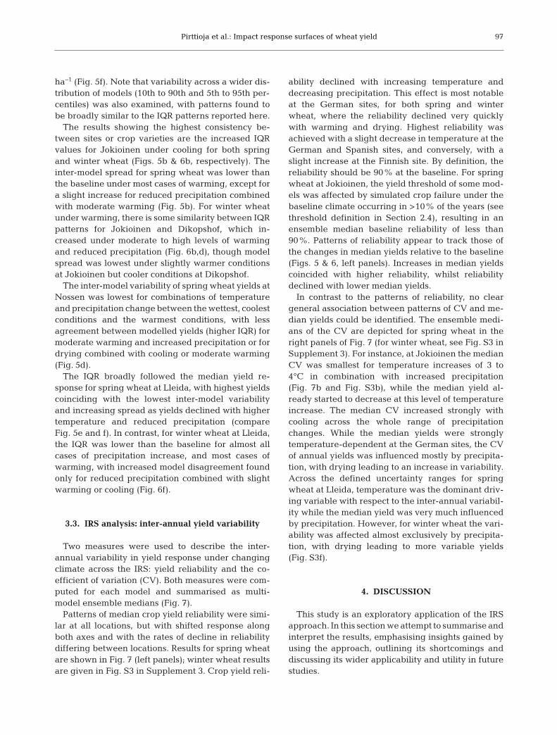
ability declined with increasing temperature anddecreasing precipitation. This effect is most notableat the German sites, for both spring and winterwheat, where the reliability declined very quicklywith warming and drying. Highest reliability wasachieved with a slight decrease in temperature at theGerman and Spanish sites, and conversely, with aslight increase at the Finnish site. By definition, thereliability should be 90% at the baseline. For springwheat at Jokioinen, the yield threshold of some mod-els was affected by simulated crop failure under thebaseline climate occurring in >10% of the years (seethreshold definition in Section 2.4), resulting in anensemble median baseline reliability of less than90%. Patterns of reliability appear to track those ofthe changes in median yields relative to the baseline(Figs. 5 & 6, left panels). Increases in median yieldscoincided with higher reliability, whilst reliabilitydeclined with lower median yields.

In contrast to the patterns of reliability, no cleargeneral association between patterns of CV and me-dian yields could be identified. The ensemble medi-ans of the CV are depicted for spring wheat in theright panels of Fig. 7 (for winter wheat, see Fig. S3 inSupplement 3). For instance, at Jokioinen the medianCV was smallest for temperature in creases of 3 to4°C in combination with increased precipitation(Fig. 7b and Fig. S3b), while the median yield al -ready started to decrease at this level of temperatureincrease. The median CV increased strongly withcooling across the whole range of precipitationchanges. While the median yields were strongly temperature-dependent at the German sites, the CVof annual yields was influenced mostly by precipita-tion, with drying leading to an increase in variability.Across the defined uncertainty ranges for springwheat at Lleida, temperature was the dominant driv-ing variable with respect to the inter-annual variabil-ity while the median yield was very much influencedby precipitation. However, for winter wheat the vari-ability was affected almost exclusively by precipita-tion, with drying leading to more variable yields(Fig. S3f).

4. DISCUSSION

This study is an exploratory application of the IRSapproach. In this section we attempt to summarise andinterpret the results, emphasising insights gained byusing the approach, outlining its shortcomings anddiscussing its wider applicability and utility in futurestudies.

97

Clim Res 65: 87–105, 2015

4.1. Ensemble wheat model responses

It has been argued that the use of a model ensem-ble increases the robustness of simulated yield esti-mates compared to using individual models, as theratio of signal (average change) to noise (variation)increases with the number of models, while errors inindividual models tend to cancel each other out(Asseng et al. 2013). The IRS plots offer a consensusview of how models simulate the joint effects of tem-perature and precipitation changes on wheat yields.Since models differ in their representation of key

processes, it can be difficult to disentangle the relativeinfluence of these 2 climatic variables on yield re -sponse across such a large and diverse set of models.Here, the results are interpreted by treating tempera-ture and precipitation effects in turn.

4.1.1. Temperature-related effects

Average yields and development. Temperaturesoutside those typically experienced can cause signif-icant reductions in yields through various processes

98

Temperature change (°C)

Temperature change (°C)

Temperature change (°C)

Temperature change (°C)

Pre

cip

itatio

n ch

ange

(%)

Pre

cip

itatio

n ch

ang

e (%

)P

reci

pita

tion

chan

ge

(%)

–2 0 2 4 6 8

–40

–20

0

20

40

–2 0 2 4 6 8

–40

–20

0

20

40

–2 0 2 4 6 8

–40

–20

0

20

40

Temperature change (°C) Temperature change (°C)

–2 0 2 4 6 8

–40

–20

0

20

40

–2 0 2 4 6 8

–40

–20

0

20

40

Pre

cip

itatio

n ch

ange

(%)

Pre

cip

itatio

n ch

ang

e (%

)P

reci

pita

tion

chan

ge

(%)

–2 0 2 4 6 8

–40

–20

0

20

40

Yield reliability(%)

CV of yield(%)

(a) Finland

1

10

20

30

40

40

50

60

70

80 90

1

10

20

30

40

50

60

70

80

90

100

(b) Finland

25

30

35

35

35

40

45

75

15

20

25

30

35

40

45

50

75

100

(c) Germany

1 10

20

30

40

50 60

70

80

90

100

(d) Germany 15

20

25

30

(e) Spain

10

20

30

40

50

60 70

80

90

(f) Spain

25

25 30

30

35

35

Fig. 7. Ensemble medians of yield reliability, defined as the percentage of years when DM grain yield (kg ha−1) is above the 10thpercentile of the baseline yield (left-hand panels), and of coefficients of variation (CV) of annual yields (right-hand panels), forspring wheat under changes in temperature and precipitation relative to the 1981−2010 baseline for 24 crop models at (a,b)

Jokioinen, Finland, and 25 models at (c,d) Nossen, Germany and (e,f) Lleida, Spain

Pirttioja et al.: Impact response surfaces of wheat yield

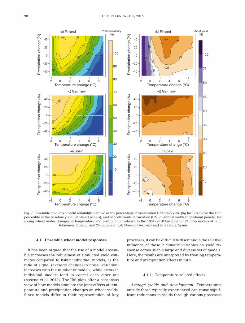
at different development stages (Asseng et al. 2014).Wheat is best suited to a cool climate with an opti-mum temperature range of 17 to 23°C over the entiregrowing season, although cultivar-specific differ-ences exist (Porter & Gawith 1999). Fig. 8a sum-marises the model ensemble temperature responsesfor winter wheat at all 3 sites assuming baseline pre-cipitation (combining information from IRSs inFig. 6). The equivalent plot for spring wheat is givenin Fig. S4a in Supplement 4 at www. int-res. com/ articles/ suppl/ c065 p087 _ supp. pdf.

Responses at all sites showed decreases in yieldswith warming. This is because present-day cultivarsat each site have been bred and selected to developand mature under ambient conditions. Warming ac -celerates plant phenology such that crops mature ear-lier, the grain filling period shortens and dry matteraccumulation is reduced, resulting in lower yields.While baseline temperatures were close to optimal forlocal cultivars under Finnish conditions, yields bene-fited from cooling at the German and Spanish sites.This suggests that adoption of later-maturing cultivarswith higher temperature requirements might alreadybe advantageous at those sites, and increasingly sounder future warming.

A decrease in yields with warming is consistentwith empirical studies of observed wheat yield trendsworldwide (Lobell & Field 2007). It is also in line withprevious multi-model studies for constant CO2 levels(Asseng et al. 2013, 2014). For example, the median30 yr mean yield response of autumn-sown wheat toa temperature increase of 6°C relative to 1981−2010

at a site in the Netherlands was −26% (Asseng et al.2013). This compares to −23%, −28% and −28% atJokioinen, Dikopshof and Lleida, respectively(Fig. 8a). Spring wheat yields were more sensitive totemperature in our results (respective values are−28%, −34% and −37% for the same 6°C warming;see Fig. S4a in Supplement 4) and the largest reduc-tions were also found in the Asseng et al. (2013) studyfor spring wheat yields in Argentina (−39%).

Harvest cut-off. Cooling had a strong effect onmodelled yields at Jokioinen, due to a failure of cropsto mature before the harvest cut-off date duringcooler baseline years in many models. Crop failuressimultaneously reduced the 30 yr mean yields whileincreasing inter-annual yield variability. The cut-offdate was introduced to avoid model simulations fromcontinuing unrealistically into a subsequent growingseason. However, its precise timing is open to debate,as well as the assumption made to set the yield to zeroduring those years. In reality, under such conditionssome farmers might still manage to salvage a crop.

High temperature extremes. The upper lethal tem-perature limit for wheat and its standard error is re-ported as 47.5 ± 0.5°C (Porter & Gawith 1999). Esti-mates from the same source of maximum temperatureabove which growth ceases are considerably lowerthan this, varying with phenological phase (32.7 ±0.9°C from sowing to emergence, 31.0°C around an-thesis and 35.4 ± 2.0°C during grain filling). Extremeheat events that exceed the maximum temperaturelimits are already observed occasionally at all sites.Moreover, with the IRS range of temperature sensi-

99

a

Temperature change (°C)

Yie

ld (%

bas

elin

e)

●

●

●

●

●

●

● NetherlandsFinlandGermanySpain

Median IQR Asseng et al. 2013

0

50

100

150

0

50

100

150 b

Precipitation change (%)

FinlandGermanySpain

Median IQR

−50 −40 −30 −20 −10 0 10 20 30 40 50−2 −1 0 1 2 3 4 5 6 7 8 9

Fig. 8. Ensemble median response (solid lines) and inter-quartile range (IQR; coloured bands) of period-mean dry matter win-ter wheat yield (%) relative to the baseline (1981− 2010) climate across 26 crop models at Jokioinen, Finland, Dikopshof, Ger-many and Lleida, Spain for changes in: (a) temperature with baseline precipitation, and (b) precipitation with baseline temper-ature. Baseline values are scaled to 100%. Coloured points and error bars are median and IQR model ensemble responses for

a site in the Netherlands, from Asseng et al. (2013)

Clim Res 65: 87–105, 2015100

tivity extending to +9°C warming, severe restrictionson growth should be expected to show in the modelresults. However, not all models applied in this studyaccount for specific heat stress impacts (Table S1 inSupplement 1), even though they may be used in cli-mate change studies. Regardless, it is difficult to dis-tinguish between heat-related impacts and otheryield-reducing stresses from these ensemble results.At Lleida, there are some instances of daily maximaexceeding the lethal limit, though with a shortenedgrowth period these occurred well after modelledharvest for present-day cultivars. However, tempera-tures of this magnitude would impose an absoluteconstraint on wheat viability during the summermonths if longer-season cultivars were to be consid-ered as an adaptation option.

Vernalisation. Increased temperature can also af -fect vernalisation, the chilling requirement of certainwinter wheat varieties that is obligatory for flower-ing. The optimum temperature for vernalisation isgiven as 4.9 ± 1.1°C with a maximum temperature of15.7 ± 2.6°C, after which vernalisation does not occurand no yield is produced (Porter & Gawith 1999).During some seasons under the high-end tempera-ture changes, requirements for vernalisation werenot met, which should result in crop failure. A fewindividual models showed this effect in some yearsfor winter wheat at Lleida (not shown), though mostmodels that simulate vernalisation (cf. Table S1 inSupplement 1) did not indicate complete crop failure.

Inter-model variability. Changes in inter-modelvariability across the IRS are determined in largemeasure by responses under baseline conditions. Thebaseline IQR at Lleida was substantially greater (bybetween 55 and 70%) for both crop varieties than atthe other 2 sites, while median yields at Lleida wererelatively low (e.g. compare the width of the colouredbands in Fig. 8a). With modelled median yieldsdeclining under warming, there is little scope for theIQR to increase significantly at Lleida, in contrast tothe German and Finnish sites, where baseline IQRwas lower. The spread of spring wheat yields nar-rowed with warming and unchanged precipitation atthe Finnish and German sites (Fig. S4a in Supplement4), while modelled winter wheat yields diverged withgreater warming (Fig. 8a). This suggests differingmodel treatment of temperature effects on overwin-tering crops (e.g. through vernalisation). Divergentyield responses to cooling at Joki o inen are attributa-ble to harvest failure occurrence in some models.

Inter-annual variability and yield reliability. IRSpatterns of modelled yield reliability under changingclimate were strongly governed by the baseline yield

response at different sites, which was used to definethe threshold yield (lowest 10th percentile). Climaticconditions were most favourable, median yields high-est, and inter-annual variability (based on the CV)lowest under the baseline climate at the 2 Germansites. While cooling improves reliability, incrementsof warm ing reduced modelled yields below the yieldthreshold and reliability fell more rapidly at the Ger-man sites than at the Finnish and Spanish sites, eventhough absolute yield levels were still higher and theCV generally lower. Cooling reduced yield reliabilityfor both crop varieties at Jokioinen, due to more fre-quent harvest failure, whilst general yield reductionsdue to shortened development phases explain the de-cline in reliability under warming climate. Warmingclimate had the least effect on reliability at Lleida, es-pecially for winter wheat, even accounting for vernal-isation effects. Here, the baseline modelled annualyields were already highly variable, and the simu-lated response of local cultivars appears to be moretolerant to high temperatures in most models than atthe German and Finnish sites.

4.1.2. Precipitation-related effects

Average yields. In the great majority of models inthe ensemble, water availability had no effect on cropdevelopment rate (cf. Table S1 in Supplement 1), sothe primary effect of precipitation change on grainyield is through limitations on growth. Rain-fed wheatyields were susceptible to moisture deficiency underall climatic regimes, but particularly so at the driestlocations. Hence, there was a positive relationshipbetween median yields and precipitation at all sitesin the transect, with the strongest effect at Lleida(Fig. 8b). This was expressed most strongly at tem-perature levels close to the baseline, and was pro-gressively reduced under increasing warming. Thelatter effect is due, in part, to reduced exposure towater deficits during a shortened growth period, aswell as the confounding effect of higher tempera-tures on water deficiency through enhanced evapo-transpiration.

Inter-model variability. For both crop varieties,models appear to agree less in their responses to re -ductions in precipitation than to increases, suggestinga diversity of approaches being used to treat yieldresponses to water deficit (e.g. see Fig. 4). Assumingun changed baseline temperatures, the level of agree -ment in modelled yields across the ensemble, de -scribed by the IQR, showed convergence with in -creasing precipitation for spring wheat at all sites

Pirttioja et al.: Impact response surfaces of wheat yield

(Fig. S4b in Supplement 4), but was little affected byprecipitation change for winter wheat (Fig. 8b). Thislatter result, considered alongside the divergence inmodelled yields under warming (Fig. 8a), suggeststhat the process representation of high temperatureresponses in winter wheat may be contributinggreater uncertainty to multi-model yield estimatesthan that of responses to water availability. Forspring wheat, especially at sites in Germany and Fin-land where no overwintering is involved, models ap -pear to converge in their estimates of responses toboth warmer and wetter conditions (Fig. S4a,b).

Inter-annual variability and yield reliability. Thesensitivity of yield reliability to precipitation was sim-ilar to that of median yields for both crop varieties,with reduced precipitation leading to an increasedfrequency of outcomes below the yield threshold inline with a general yield decline at all sites. In con-trast, annual yield variability expressed by the CVvaried considerably among crop varieties and sites.While the median CV for spring wheat at Lleida wasdominated by temperature change, for other cases inregions of the IRS where results showed an increasedCV with declining precipitation, it is likely that yielddeclines in dry years may be dominating the medianyield response. This is especially true at Dikopshoffor winter wheat, where precipitation exerted thedominant constraint on inter-annual variability re -gardless of temperature changes (Fig. 7d). It is worthnoting in this context that there was also less agree-ment between models across the IRS for winterwheat yield responses at Dikopshof (Fig. 6d) than forany other crop variety or site, suggesting that moreanalysis is needed of responses to temperature andprecipitation change during anomalous weatheryears in order to understand better the differencesbe tween models.

4.2. Applicability of the IRS approach

4.2.1. Shortcomings

Given the exploratory nature of this study, and theneed to limit the number of model simulations re -quired of modelling groups, numerous simplifica-tions were required in the modelling protocol agreedfor this initial study. These may have compromisedthe realism and real world applicability of someresults.

(1) The calibration data provided for modellerscomprised, in most cases, only a few data points andan insufficient level of detail to allow for rigorous cal-

ibration (van Keulen & Wolf 1986, Wallach et al.2013). With such restricted calibration material, largeuncertainties in estimates of impact variables such asyield can result (Makowski et al. 2002, Palosuo et al.2011, Watson et al. 2014). Aside from the limitationsin quantity of data, there are also numerous choicesavailable in the approaches used to calibrate models.The effects of such calibration decisions can be com-pared explicitly in this study for those cases in whichthe same model version has been applied by differ-ent modelling groups (for example, compare resultsin Table 2 between ID numbers 7 and 8 and 25 and26, respectively). Moreover, in terms of evaluation,the short time series of calibration data also made itimpossible to conduct a statistically meaningful com-parison of simulated versus observed yields at sites.

(2) Some of the climatic constraints to wheat pro-duction require more processes to be accounted forthan are commonly treated in models. For instanceonly about half of the 24 models applied in this studyaccount for specific heat stress impacts such as floretmortality at anthesis or leaf senescence (Challinor etal. 2005, Alderman et al. 2014). Surplus water is notaccounted for in any of the models, though excess soilmoisture can create several issues. For example, ifthis excess moisture occurs between sowing and theend of tillering, it can reduce the number of kernelsper head and hence the number of tillers per plantand grain yield (Trnka et al. 2014), and heavy precipi-tation close to maturity may cause lodging of grainand yield losses (Peltonen-Sainio et al. 2011, Trnka etal. 2014). In addition, waterlogging can cause difficul-ties of access for machinery to farmland, affectingworkability and trafficability (Jones & Thomasson1985). Such omissions can lead to the over-estimationof yields compared to those observed and to discrep-ancies in capturing inter-annual variations, in partic-ular during extreme weather years. Similarly, re-ini-tialising the simulations at the beginning of eachyear, always with the same assumption of soil mois-ture, may affect simulation results when long-termtrends in soil moisture are not accounted for.

(3) Inter-annual variability has been assessed bothby presenting the full modelled yield distributions(CV) and by referencing yields against a thresholdlevel (reliability). However, by reporting only medianresults of these measures, information may havebeen lost from the suite of multi-model outcomes.Ana lysis of percentiles towards the tails of the en -semble results could also be considered, though ad -ditional insights may require closer scrutiny of ano - malous weather-years (e.g. cool, warm, wet or dryseasons) during the baseline period.

101

Clim Res 65: 87–105, 2015102

(4) The IRS depicts responses for temperature andprecipitation changes alone. As these change, allother weather variables are assumed to remain fixed,even though the resulting combinations may be phys-ically implausible (for example, model discrepanciesin the relationship between temperature and humidityare described in Section 2.2.2). Temperature and pre-cipitation changes were applied uniformly throughoutthe year, whereas in reality, climate model projectionsindicate that future climate changes will vary season-ally, and that this seasonal pattern of change varies byregion (IPCC 2013a). Future changes of climate willalso be associated with altered CO2 levels, whichthemselves can be expected to affect crop growth andwater use. CO2 was fixed at 360 ppm in this study, soresults for changed climate may not reflect realisticcrop re sponses that can be anticipated for the future.Moreover, present-day management practices andcurrent crop cultivars, that were assumed to be fixed,would in reality certainly be modified to suit thechanging conditions. While the approach may havelimitations for analysing and discriminating betweenresponses to multiple predictors, CO2 effects can betreated by constructing IRSs for different time periods,and other key variables can be analysed through con-struction of additional bivariate IRSs, or by as sumingthat they change concurrently with the primary vari-ables (e.g. as indicated in climate model projections).

4.2.2. Utility of the approach

In this study impact response surfaces have provento be a useful device for analysing and comparingmultiple model simulations of crop yield responses tochanges in climate across a wide range of plausiblefuture conditions. IRSs also offered a useful meansfor detecting modelling, data or transcription errors.

As has been demonstrated in some earlier applica-tions (Luo et al. 2007, Fronzek et al. 2010, Wilby et al.2014), IRS plots can readily be combined with climatechange projections (here, of annual temperature andprecipitation change), where responses for any sce-nario-based combination of changes based on cli-mate models should logically fall somewhere withinthis response space. We have illustrated this by plot-ting recent climate change projections for the end ofthe century over central Europe (IPCC 2013a) ontothe 30 yr mean plot of Fig. S2 in Supplement 3. Thisidea can be extended if projections of temperatureand precipitation change are presented probabilisti-cally (e.g. see Harris et al. 2010). By superimposing ajoint probability distribution onto an IRS, it becomes

feasible to estimate the likelihood of exceeding a cer-tain impact threshold, such as a critical level of yieldas defined on the response surface (Fronzek et al.2010, Børgesen & Olesen 2011, Ferrise et al. 2011).Such analyses are planned in ongoing studies, whichalso consider CO2 level and seasonality that arerequired for more realistic projections of future yield(see Section 4.2.1).

The results presented here, along with follow-upstudies, may help to identify model deficiencies thatreflect shortcomings in process understanding orrepresentation. Some of the other output variablesgenerated in the modelling exercise, such as pheno -logy, water use and total biomass, could be used tolook for clues that might explain differences in mod-elled yield responses. There are several other poten-tial applications of the IRS approach to crop model-ling that also remain to be explored. IRSs can beconstructed that explore within-model parameter un -certainties alongside between-model structural un -certainties of the type examined in this study (e.g.Fronzek et al. 2011). IRSs can also be used to analyseeffects of seasonal weather anomalies through con-sideration of year-to-year responses (cf. Fronzek2013).

Building on the experiences gained here, a follow-up study using the same data will explore methods ofclassifying IRS responses and how different patternsof impact response described in Section 3.2 might berelated to known characteristics of the models. An -other study, also for wheat, involving many of thesame models, will endeavour to introduce more real-ism into the model simulations. The IRS approachcan then be used to assess the potential effectivenessof farm-level adaptation measures, such as alteredsowing date and cultivar selection.

Finally, this analysis has focused on comparingthe behaviour of process-based wheat models underchanged climate at sites in Europe. However, in prin-ciple the IRS approach can be applied in examiningclimate change impacts for any system or activity thatcan be represented by causal models that are sensi-tive to 2 dominant variables.

5. CONCLUSIONS

In this study we have reported a novel approach forinter-comparing simulated impacts of climate changeacross a large ensemble of models and a wide rangeof plausible changes in climate at diverse locations inEurope, using impact response surfaces (IRSs). Theapproach appears to offer an effective method of por-

Pirttioja et al.: Impact response surfaces of wheat yield 103

traying model behaviour under changing climate, aswell as numerous advantages for analysing, compar-ing and presenting results from multi-model ensem-ble simulations.

In spite of the simplified assumptions required forundertaking multiple simulations, some clear ten-dencies emerged from this analysis:

• Over the range of climate changes considered,median modelled yields were more sensitive to tem-perature change than to precipitation change at theFinnish site, while sensitivities were more evenly dis-tributed between temperature and precipitation atthe German and Spanish sites.

• From the model analysis, assuming current CO2

levels, we can conclude that average yields of cur-rent wheat cultivars decline with higher tempera-tures and decreased precipitation, but benefit fromincreased precipitation.

• Warming alone, under baseline precipitation,induced remarkably similar rates of median yielddecline (5−7% per 1°C, see Supplement 4) acrosssites and crop varieties.

• Corresponding responses to precipitation underbaseline temperature were more varied (1−10% per10% precipitation change).

• Individual model behaviour may depart mark -edly from the median response.

While IRSs are very helpful for summarising multi-ple model simulations, complementary approaches(e.g. focusing on individual model responses or onanomalous weather-years) are still required for gain-ing a fuller appreciation of the reasons for modelbehaviour. Furthermore, the bivariate nature of theIRS analysis may obscure responses attributable toother key explanatory variables, though these toocan potentially be explored using other methods.

Finally, we have shown how the IRS approach canfacilitate an examination of other statistical charac-teristics of the ensemble response, such as the inter-model and inter-annual variability. Plots such as theIQR can assist in highlighting aspects of the sensitiv-ity to climate for which models exhibit divergent be-haviour. The reliability and CV plots are instructivein revealing sensitivities of annual responses whichmay differ from period-average responses. Together,these help to pinpoint processes, such as heat stress,vernalisation or drought, that may require further at-tention in future model development.

Acknowledgements. This work was conducted in the con-text of CROPM, the crop modelling component of MACSUR(Modelling European Agriculture with Climate Change forFood Security), a project launched by the Joint Research

Programming Initiative (JPI) on Agriculture, Food Securityand Climate Change (FACCE – Rötter et al. 2013, Ewert etal. 2014). The authors acknowledge financial support fromthe following sources: FACCE JPI, MACSUR, the Academyof Finland for the A-LA-CARTE (decisions: 140806 and140870) and PLUMES (decisions: 277276 and 277403) pro-jects, the European Commission Seventh Framework Pro-gramme IMPRESSIONS project (grant agreement no.603416), the Italian Ministry of Agriculture (AGROSCE-NARI Project), the Italian Ministry of Research (FIRB 2012,RBFR12B2K4_004), the German Federal Office for Agricul-ture and Nutrition, the MTT strategic project MODAGS, theMULCLIVAR project from the Spanish Ministerio de Eco -nomía y Competitividad (MINECO) CGL2012-38923-C02-02, the Belgium funding agency DGO-3(SPW− Belgium),University of Sassari, Polish National Centre for Researchand Development, the German Federal Ministries of Educa-tion and Research, and Food and Agriculture (grant no.2812ERA115), the Czech National Agency for AgriculturalResearch (project no. QJ1310123) and KONTAKT projectno. LD13030.

LITERATURE CITED

Abeledo LG, Savin R, Slafer GA (2008) Wheat productivityin the Mediterranean Ebro Valley: analyzing the gapbetween attainable and potential yield with a simulationmodel. Eur J Agron 28: 541−550

Alderman P, Quilligan E, Asseng S, Ewert F, Reynolds M(2014) Proc Workshop Model Wheat Response HighTemp. CIMMYT, El Batán, Mexico, 19−21 June 2013

Angulo C, Rötter R, Lock R, Enders A, Fronzek S, Ewert F(2013) Implication of crop model calibration strategies forassessing regional impacts of climate change in Europe.Agric For Meteorol 170: 32−46

Asseng S, Ewert F, Rosenzweig C, Jones JW and others(2013) Uncertainty in simulating wheat yields under cli-mate change. Nat Clim Change 3: 827−832

Asseng S, Ewert F, Martre P, Rötter RP and others (2014) Ris-ing temperatures reduce global wheat production. NatClim Change 5: 143–147

Becker R, Chambers J, Wilks A (1988) The new S language.Wadsworth & Brooks/Cole, Pacific Grove, CA

Børgesen CD, Olesen JE (2011) A probabilistic assessmentof climate change impacts on yield and nitrogen leachingfrom winter wheat in Denmark. Nat Hazards Earth SystSci 11: 2541−2553

Cartelle J, Pedró A, Savin R, Slafer GA (2006) Grain weightresponses to post-anthesis spikelet-trimming in an oldand a modern wheat under Mediterranean conditions.Eur J Agron 25: 365−371

Challinor A, Wheeler T, Craufurd P, Slingo J (2005) Simula-tion of the impact of high temperature stress on annualcrop yields. Agric For Meteorol 135: 180−189

Challinor AJ, Simelton ES, Fraser ED, Hemming D, CollinsM (2010) Increased crop failure due to climate change: assessing adaptation options using models and socio-economic data for wheat in China. Environ Res Lett 5: 034012

Challinor A, Martre P, Asseng S, Thornton P, Ewert F(2014a) Making the most of climate impacts ensembles.Nat Clim Change 4: 77−80

Challinor AJ, Watson J, Lobell DB, Howden SM, Smith DR,Chhetri N (2014b) A meta-analysis of crop yield under

Clim Res 65: 87–105, 2015

climate change and adaptation. Nat Clim Change 4: 287−291

Cleveland WS (1993) Visualizing data. Hobart Press, Sum-mit, NJ

Craufurd PQ, Vadez V, Krishna Jagadish SV, Vara PrasadPV, Zaman-Allah M (2013) Crop science experiments de -signed to inform crop modeling. Agric For Meteorol 170: 8−18

Diaz-Nieto J, Wilby RL (2005) A comparison of statisticaldownscaling and climate change factor methods: im -pacts on low flows in the River Thames, United Kingdom.Clim Change 69: 245−268

Easterling WE, Aggarwal PK, Batima P, Brander KM andothers (2007) Food, fibre and forest products. In: ParryML, Canziani OF, Palutikof JP, van der Linden PJ, Han-son CE (eds) Climate change 2007: impacts, adaptationand vulnerability. Contribution of Working Group II tothe Fourth Assessment Report of the IntergovernmentalPanel on Climate Change. Cambridge University Press,Cambridge, p 273−313

Ewert F, Rötter R, Bindi M, Webber H and others (2014)Crop modelling for integrated assessment of risk to foodproduction from climate change. Environ Model Softw,doi: 10.1016/j.envsoft.2014.12.003

Ferrise R, Moriondo M, Bindi M (2011) Probabilistic assess-ments of climate change impacts on durum wheat in theMediterranean region. Nat Hazards Earth Syst Sci 11: 1293−1302

Fronzek S (2013) Climate change and the future distributionof palsa mires: ensemble modelling, probabilities anduncertainties. Monogr Boreal Environ Res No. 44, http: //hdl.handle.net/10138/40184

Fronzek S, Carter TR, Raisanen J, Ruokolainen L, Luoto M(2010) Applying probabilistic projections of climatechange with impact models: a case study for sub-arcticpalsa mires in Fennoscandia. Clim Change 99: 515−534

Fronzek S, Carter TR, Luoto M (2011) Evaluating sources ofuncertainty in modelling the impact of probabilistic cli-mate change on sub-arctic palsa mires. Nat HazardsEarth Syst Sci 11: 2981−2995

Gitay H, Brown S, Easterling W, Jallow B and others (2001)Ecosystems and their goods and services. In: McCarthyJJ, Canziani OF, Leary NA, Dokken DJ, White KS (eds)Climate change 2001: impacts, adaptation, and vulnera-bility. Contribution of Working Group II to the ThirdAssessment Report of the Intergovernmental Panel onClimate Change. Cambridge University Press, Cam-bridge, p 235−242

Hanasaki N, Masutomi Y, Takahashi K, Hijioka Y, HarasawaH, Matsuoka Y (2007) Development of a global waterresources scheme for climate change policy supportmodels. Environmental systems research. Jpn Soc CivEng 35: 367−374 (in Japanese)

Harris GR, Collins M, Sexton DMH, Murphy JM, Booth BBB(2010) Probabilistic projections for 21st century Euro-pean climate. Nat Hazards Earth Syst Sci 10: 2009−2020

Iizumi T, Yokozawa M, Nishimori M (2011) Probabilisticevaluation of climate change impacts on paddy rice pro-ductivity in Japan. Clim Change 107: 391−415

IPCC (2013a) Annex I: Atlas of global and regional climateprojections [van Oldenborgh GI and others]. In: StockerTF, Quin D, Plattner GK, Tignor M and others (eds) Cli-mate change 2013: the physical science basis. Contribu-tion of Working Group I to the Fifth Assessment Report ofthe Intergovernmental Panel on Climate Change. Cam-

bridge University Press, Cambridge, p 1311−1393IPCC (2013b) Annex II: Climate system scenario tables

[Prather M and others]. In: Stocker TF, Quin D, PlattnerGK, Tignor M and others (eds) Climate change 2013: thephysical science basis contribution of Working Group I tothe Fifth Assessment Report of the IntergovernmentalPanel on Climate Change. Cambridge University Press,Cambridge, p 1395−1445

Jamieson PD, Porter JR, Goudriaan J, Ritchie JT, van KeulenH, Stol W (1998) A comparison of the models AFR-CWHEAT2, CERES-Wheat, Sirius, SUCROS2 andSWHEAT with measurements from wheat grown underdrought. Field Crops Res 55: 23−44

Jones RJA, Thomasson AJ (1985) An agroclimatic databankfor England and Wales. Tech Monogr No. 16, Soil surveyof England and Wales, Harpenden

Lobell DB, Field CB (2007) Global scale climate−crop yieldrelationships and the impacts of recent warming. Envi-ron Res Lett 2: 014002

Luo Q, Bellotti W, Williams M, Cooper I, Bryan B (2007) Riskanalysis of possible impacts of climate change on SouthAustralian wheat production. Clim Change 85: 89−101

Makowski D, Wallach D, Tremblay M (2002) Using aBayesian approach to parameter estimation; comparisonof the GLUE and MCMC methods. Agronomie 22: 191−203

Metzger M, Bunce R, Jongman R, Mücher C, Watkins J(2005) A climatic stratification of the environment ofEurope. Glob Ecol Biogeogr 14: 549−563

Monfreda C, Ramankutty N, Foley JA (2008) Farming theplanet. 2. Geographic distribution of crop areas, yields,physiological types, and net primary production in theyear 2000. Global Biogeochem Cycles 22: GB1022, doi: 10.1029/2007GB002947

Palosuo T, Kersebaum KC, Angulo C, Hlavinka P and others(2011) Simulation of winter wheat yield and its variabilityin different climates of Europe: a comparison of eightcrop growth models. Eur J Agron 35: 103−114

Peltonen-Sainio P, Jauhiainen L, Hakala K (2011) Cropresponses to temperature and precipitation according tolong-term multi-location trials at high-latitude condi-tions. J Agric Sci 149: 49−62

Porter J (1993) AFRCWHEAT2: a model of the growth anddevelopment of wheat incorporating responses to waterand nitrogen. Eur J Agron 2: 69−82

Porter JR, Gawith M (1999) Temperatures and the growthand development of wheat: a review. Eur J Agron 10: 23−26

Porter JR, Xie L, Challinor A, Cochrane K and others (2014)Food security and food production systems. In: Field CBand others (eds) Climate change 2014: impacts, adapta-tion and vulnerability. Contribution of Working Group IIto the Fifth Assessment Report of the IntergovernmentalPanel on Climate Change. Cambridge University Press,Cambridge, p 485−533

R Core Team (2013) R: a language and environment for sta-tistical computing. R Foundation for Statistical Comput-ing, Vienna. www.R-project.org/

Rosenzweig C, Jones JW, Hatfield JL, Ruane AC and others(2013) The agricultural model intercomparison andimprovement project (AgMIP): protocols and pilot stud-ies. Agric For Meteorol 170: 166−182

Rosenzweig C, Elliott J, Deryng D, Ruane AC and others(2014) Assessing agricultural risks of climate change inthe 21st century in a global gridded crop model inter-

104

Pirttioja et al.: Impact response surfaces of wheat yield 105

comparison. Proc Natl Acad Sci USA 111: 3268−3273Rötter RP (2014) Agricultural impacts: robust uncertainty.

Nat Clim Change 4: 251−252Rötter RP, Carter TR, Olesen JE, Porter JR (2011) Crop- climate

models need an overhaul. Nat Clim Change 1: 175−177Rötter RP, Ewert F, Palosuo T, Bindi M and others (2013)

Challenges for agro-ecosystem modelling in climatechange risk assessment for major European crops andfarming systems. Proc Impacts World 2013 Conf, Pots-dam, 27–30 May 2013, p 555−564

Ruane AC, McDermid S, Rosenzweig C, Baigorria GA andothers (2014) Carbon−temperature−water change analy-sis for peanut production under climate change: a proto-type for the AgMIP Coordinated Climate–Crop Model-ing Project (C3MP). Glob Chang Biol 20: 394−407

Trnka M, Rötter RP, Ruiz-Ramos M, Kersebaum KC and oth-ers (2014) Adverse weather conditions for Europeanwheat production will become more frequent with cli-mate change. Nat Clim Change 4: 637−643

van Ittersum M, Rabbinge R (1997) Concepts in productionecology for analysis and quantification of agriculturalinput-output combinations. Field Crops Res 52: 197−208

van Ittersum MK, Leffelaar PA, Van Keulen H, Kropff MJ,Bastiaans L, Goudriaan J (2003) On approaches andapplications of the Wageningen crop models. Eur JAgron 18: 201−234

van Keulen H, Wolf J (1986) Modelling of agricultural pro-

duction: weather, soils and crops. PUDOC, WageningenWallach D, Makowski D, Jones JW, Brun F (2013) Working

with dynamic crop models: methods, tools and examplesfor agriculture and environment. Academic Press, London

Watson J, Challinor AJ, Fricker TE, Ferro CA (2014) Compar-ing the effects of calibration and climate errors on a statis-tical crop model and a process-based crop model. ClimChange, doi: 10.1007/s10584-014-1264-3014-1264-3

Wetterhall F, Graham LP, Andreasson J, Rosberg J, Yang W(2011) Using ensemble climate projections to assessprobabilistic hydrological change in the Nordic region.Nat Hazards Earth Syst Sci 11: 2295−2306

White JW, Hoogenboom G, Kimball BA, Wall GW (2011)Methodologies for simulating impacts of climate changeon crop production. Field Crops Res 124: 357−368

Wilby RL, Dawson CW, Murphy C, O’Connor P, Hawkins E(2014) The Statistical DownScaling Model-Decision Cen-tric (SDSM-DC): conceptual basis and applications. ClimRes 61: 259−276

Wu L, Kersebaum KC (2008) Modeling water and nitrogeninteraction responses and their consequences in cropmodels. In: Ahuja LR, Reddy VR, Saseendran SA, Yu Q(eds) Response of crops to limited water: understandingand modeling water stress effects on plant growth pro-cesses. ASA-CSSA-SSSA, Madison, WI, p 215−249

Zadoks JC, Chang TT, Konzak CF (1974) A decimal code forthe growth stages of cereals. Weed Res 14: 415−421

Submitted: January 15, 2015; Accepted: June 22, 2015 Proofs received from author(s): August 6, 2015

➤

➤

➤

➤

➤

➤

➤

➤

➤

➤