Embed Size (px)
Citation preview
F. Calogero, On a technique to identify solvable/integrable many-body problems / Milan, 30.09.2011 / page 1 / 28
On a technique to identify solvable/integrable many-body
problems Francesco Calogero
Physics Department, University of Rome “La Sapienza” Istituto Nazionale di Fisica Nucleare, Sezione di Roma
[email protected], [email protected] Summary
The starting point is a square matrix ( )tUU ≡ , of rank N, evolving in the independent variable t (“time”) according to a solvable (or perhaps just integrable) matrix evolution equation. One then
focuses on the evolution of its N eigenvalues ( )tzz nn ≡ . This evolution generally also involves N(N−1) additional variables. In some cases via a compatible ansatz these additional variables can be expressed in terms of the N variables ( )tzz nn ≡ . Thereby one obtains a system of evolution equations
involving only the N dependent variables ( )tzz nn ≡ , which is generally interpretable as a many-body problem (characterized by Newtonian equations of motion). This approach is tersely reviewed, and several new solvable (and one integrable) many-body problems identified in this manner are reported.
F. Calogero, On a technique to identify solvable/integrable many-body problems / Milan, 30.09.2011 / page 2 / 28
Recent papers containing findings including those reported below:
- F. Calogero, “Two new solvable dynamical systems of goldfish type”, J. Nonlinear Math. Phys. 17, 397-414 (2010). DOI: 10.1142/S1402925110000970. - F. Calogero, “A new goldfish model”, Theor. Math. Phys. 167, 714-724 (2011). - F. Calogero, “Another new goldfish model”, Theor. Math. Phys. (in press). - F. Calogero, “A new integrable many-body problem”, J. Math. Phys. (in press). - F. Calogero, “New solvable many-body model of goldfish type”, J. Nonlinear Math. Phys. (submitted to, 4 September 2011). - F. Calogero, “Two quite similar matrix ODEs and the many-body problems related to them”, Proceedings of the Beppe Marmo 65th Birthdate Meeting, Int. J. Geom. Met. Mod. Phys. (in press).
F. Calogero, On a technique to identify solvable/integrable many-body problems / Milan, 30.09.2011 / page 3 / 28
A few decades ago the many-body problem of N equal particles interacting pairwise in one-dimensional space via a force proportional to the inverse cube of their separation was shown to be solvable by algebraic operations. This many-body model is generally identified by the names of the two authors who demonstrated its solvable character, firstly in a quantum context ["Schrödinger equation": F. Calogero, "Solution of the one-dimensional N-body problem with quadratic and/or inversely quadratic pair potentials", J. Math. Phys. 12, 419-436 (1971); "Erratum", ibidem 37, 3646 (1996)] and then in a classical context ["Newtonian equations of motion": J. Moser, "Three integrable Hamiltonian systems connected with isospectral deformations", Adv. Math. 16, 197-220 (1975)]. Accordingly, it will be hereafter referred to as the CM model. The Newtonian equations of motion of this prototypical many-body problem read as follows:
( ) 3
,1
2 −
≠=
−= ∑ mn
N
nmmn zzgz&&
F. Calogero, On a technique to identify solvable/integrable many-body problems / Milan, 30.09.2011 / page 4 / 28
Notation. Here the N coordinates zn≡zn(t) are the dependent variables (and below we generally assume they are complex), superimposed dots denote differentiations with respect to the (real) independent variable t ("time"), N is an arbitrary positive integer, and g2 is an arbitrary "coupling constant". Indices such as n, m, k, generally run from 1 to N, unless otherwise specified.
This model was the prototype of many subsequent developments in the theory of integrable dynamical systems: the relevant literature is vast, amounting to several hundred, possibly a few thousand, papers and tens of books, which can nowadays be easily traced via internet. An early, landmark contribution due to Olshanetsky and Perelomov [M. A. Olshanetsky and A. M. Perelomov, "Explicit solution of the Calogero model in the classical case and geodesic flows on symmetric spaces of zero curvature", Lett. Nuovo Cimento 16, 333-339 (1976)] explained the solvable character of the CM model in the classical context via the possibility to identify the N coordinates of its moving particles with the N eigenvalues of a square matrix of rank N itself evolving in time extremely simply (linearly). The time-evolution of that matrix could therefore be explicitly ascertained, and the solution of the CM many-body problem was thereby reduced to the purely algebraic task of evaluating the N eigenvalues zn≡zn(t) of an explicitly known matrix of rank N, or equivalently to finding the N zeros zn≡zn(t) of an explicitly known time-dependent polynomial of degree N in its argument z.
F. Calogero, On a technique to identify solvable/integrable many-body problems / Milan, 30.09.2011 / page 5 / 28
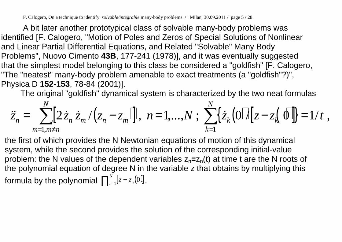
A bit later another prototypical class of solvable many-body problems was identified [F. Calogero, "Motion of Poles and Zeros of Special Solutions of Nonlinear and Linear Partial Differential Equations, and Related "Solvable" Many Body Problems", Nuovo Cimento 43B, 177-241 (1978)], and it was eventually suggested that the simplest model belonging to this class be considered a "goldfish" [F. Calogero, "The "neatest" many-body problem amenable to exact treatments (a "goldfish"?)", Physica D 152-153, 78-84 (2001)]. The original "goldfish" dynamical system is characterized by the two neat formulas
( )[ ] ( ) ( )[ ]{ } ,/10/0;,...,1,/21,1
tzzzNnzzzzzN
kkk
N
nmmmnmnn =−=−= ∑∑
=≠=
&&&&&
the first of which provides the N Newtonian equations of motion of this dynamical system, while the second provides the solution of the corresponding initial-value problem: the N values of the dependent variables zn≡zn(t) at time t are the N roots of the polynomial equation of degree N in the variable z that obtains by multiplying this
formula by the polynomial ( )[ ]∏ =−N
n nzz1
0 .
F. Calogero, On a technique to identify solvable/integrable many-body problems / Milan, 30.09.2011 / page 6 / 28
The origin of the terms “goldfish”, “goldfishing” The following quotation is from my book (F. Calogero, Isochronous systems, Oxford
University Press, 2008), in particular from its Section 4.2.2 entitled “Goldfishing”. “This terminology originated from the following description of the search for integrable
systems given by V. E. Zakharov: "A mathematician, using the dressing method to find a new integrable system, could be compared with a fisherman, plunging his net into the sea. He does not know what a fish he will pull out. He hopes to catch a goldfish, of course. But too often his catch is something that could not be used for any known to him purpose. He invents more and more sophisticated nets and equipments and plunges all that deeper and deeper. As a result he pulls on the shore after a hard work more and more strange creatures. He should not despair, nevertheless. The strange creatures may be interesting enough if you are not too pragmatic. And who knows how deep in the sea do goldfishes live?" [ V. E. Zakharov, “On the dressing method”, in: P. C. Sabatier (editor), Inverse Methods in Action, Springer, Heidelberg, 1990, pp. 602-623].”
Motivated by this poetic description of the search for integrable systems I - somewhat presumptuously (albeit with a question mark) - used the term “goldfish” in a contribution to Zakharov‘s 60th birthday meeting: F. Calogero, "The ‘neatest’ many-body problem amenable to exact treatments (a ‘goldfish’?)", Physica D 152-153, 78-84 (2001). Actually the solvable character of the prototypical goldfish model had been identified several years earlier as the simplest specimen of a solvable class of dynamical systems: F. Calogero, "Motion of Poles and Zeros of Special Solutions of Nonlinear and Linear Partial Differential Equations, and Related ‘Solvable’ Many-Body Problems", Nuovo Cimento 43B, 177-241 (1978).
F. Calogero, On a technique to identify solvable/integrable many-body problems / Milan, 30.09.2011 / page 7 / 28
Subsequently the name "goldfish" has been used for several variants of the prototypical model - which also happens to be the simplest example of the Ruijsenaars-Schneider class of integrable dynamical systems [S. N. M. Ruijsenaars and H. Schneider, "A new class of integrable systems and its relation to solitons", Ann. Phys. 170, 370-405 (1986)]. These variants are characterized by the presence in the right-hand (“forces”) side of their Newtonian equations of motion of the term in the right-hand (“forces”) side of the “goldfish” Newtonian equations of motion written above, in addition of course to additional terms. Several such models are reviewed in Section 4.2.2 (“Goldfishing”) of my last book [F. Calogero, Isochronous systems, Oxford University Press, 2008], and a few additional ones have been identified later. These findings were mainly arrived at via a generalization of the Olshanetsky and Perelomov technique (see their paper quote above, and Section 2.1.3.2 - entitled “The technique of solution of Olshanetsky and Perelomov” - of my previous book [F. Calogero, Classical many-body problems amenable to exact treatments, Springer, 2001] - a technique that in my opinion justifies the term “goldfishing” inasmuch as it calls to mind the research approach poetically described by V. E. Zakharov, as quoted above.
The solvable character of these models allows detailed analyses of their behavior, which in some cases is quite remarkable (for instance isochronous or asymptotically isochronous).
F. Calogero, On a technique to identify solvable/integrable many-body problems / Milan, 30.09.2011 / page 8 / 28
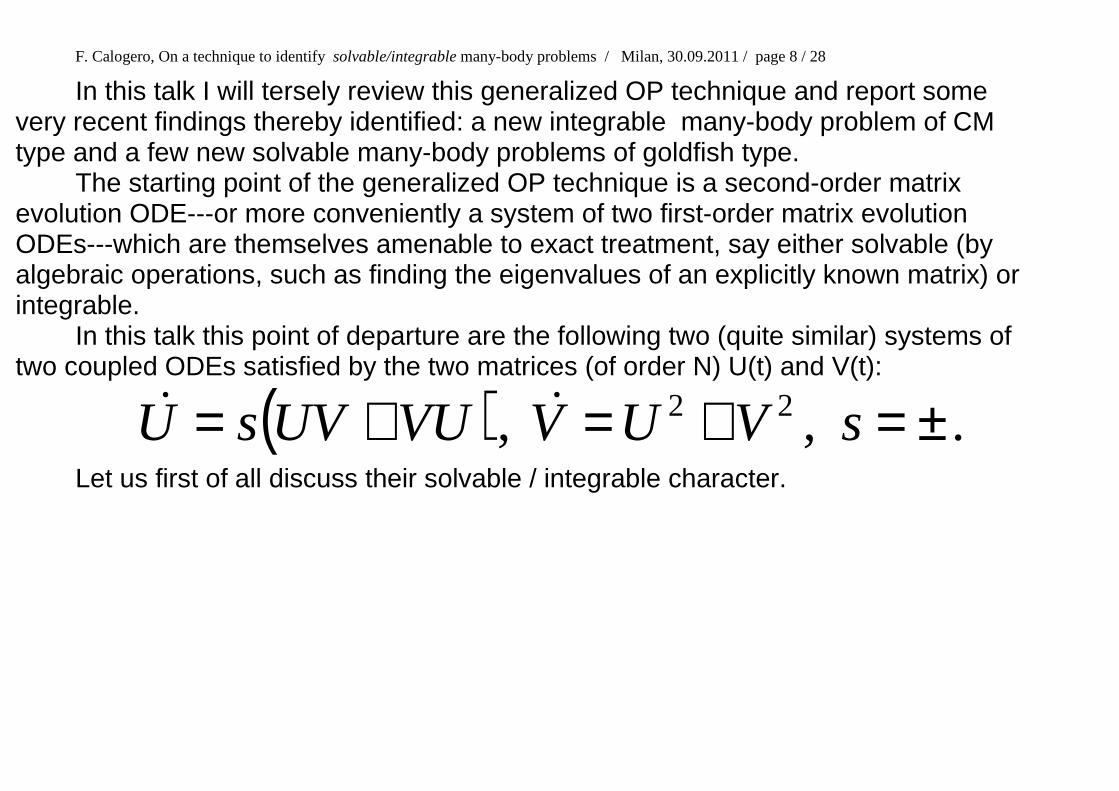
In this talk I will tersely review this generalized OP technique and report some very recent findings thereby identified: a new integrable many-body problem of CM type and a few new solvable many-body problems of goldfish type.
The starting point of the generalized OP technique is a second-order matrix evolution ODE---or more conveniently a system of two first-order matrix evolution ODEs---which are themselves amenable to exact treatment, say either solvable (by algebraic operations, such as finding the eigenvalues of an explicitly known matrix) or integrable.
In this talk this point of departure are the following two (quite similar) systems of two coupled ODEs satisfied by the two matrices (of order N) U(t) and V(t):
( ) .,, 22 ±=+=+= sVUVVUUVsU &&
Let us first of all discuss their solvable / integrable character.
F. Calogero, On a technique to identify solvable/integrable many-body problems / Milan, 30.09.2011 / page 9 / 28
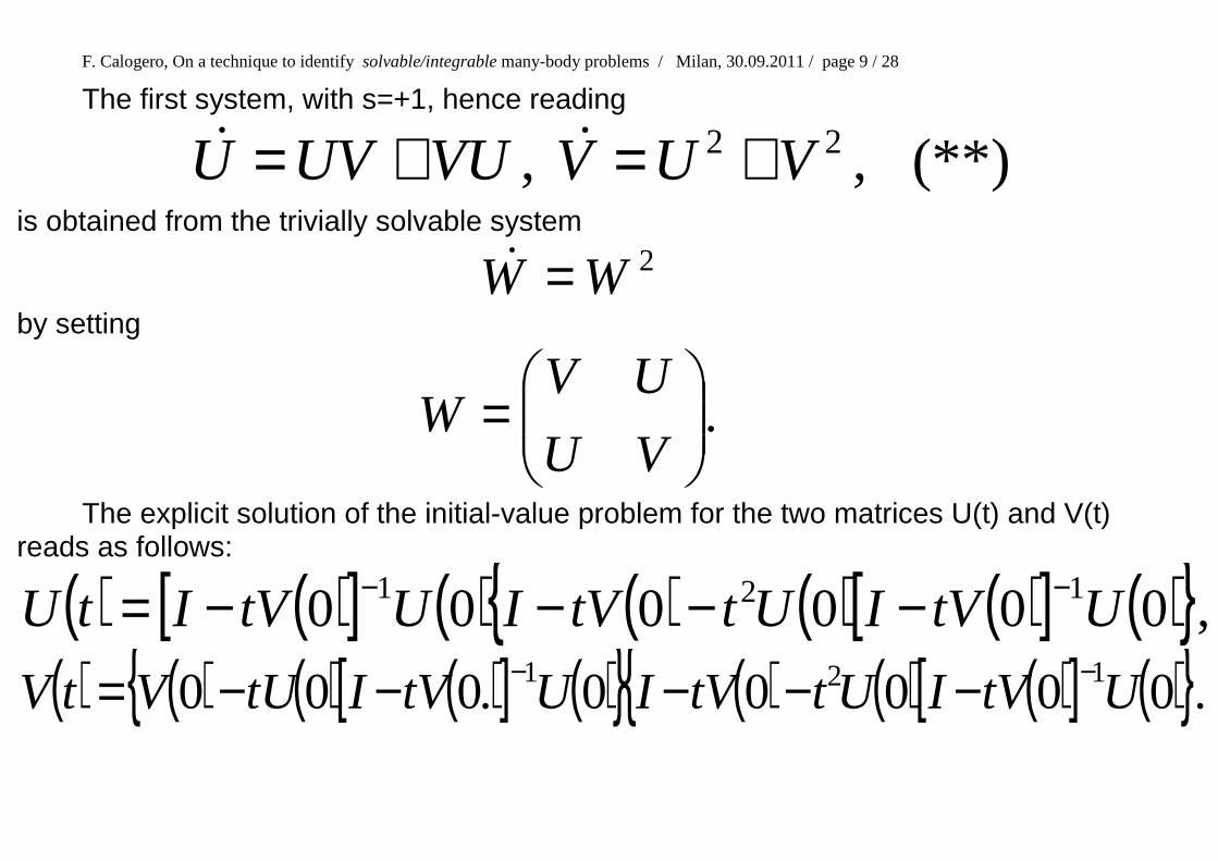
The first system, with s=+1, hence reading
(**),, 22 VUVVUUVU +=+= &&
is obtained from the trivially solvable system 2WW =&
by setting
.
=
VU
UVW
The explicit solution of the initial-value problem for the two matrices U(t) and V(t) reads as follows:
( ) ( )[ ] ( ) ( ) ( ) ( )[ ] ( ){ },000000 121 UtVIUttVIUtVItU −− −−−−=( ) ( ) ( ) ( )[ ] ( ){ } ( ) ( ) ( )[ ] ( ){ }.00000.000 121 UtVIUttVIUtVItUVtV −− −−−−−=
F. Calogero, On a technique to identify solvable/integrable many-body problems / Milan, 30.09.2011 / page 10 / 28
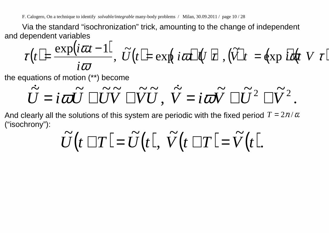
Via the standard “isochronization” trick, amounting to the change of independent and dependent variables
( ) ( ) ( ) ( ) ( ) ( ) ( ) ( )exp~
,exp~
,1exp τωτω
ωωτ VtitVUtitU
i
tit ==−=
the equations of motion (**) become
.~~~~
,~~~~~~ 22 VUViVUVVUUiU ++=++= ωω &&
And clearly all the solutions of this system are periodic with the fixed period ωπ /2=T (“isochrony”):
( ) ( ) ( ) ( ).~~,
~~tVTtVtUTtU =+=+
F. Calogero, On a technique to identify solvable/integrable many-body problems / Milan, 30.09.2011 / page 11 / 28
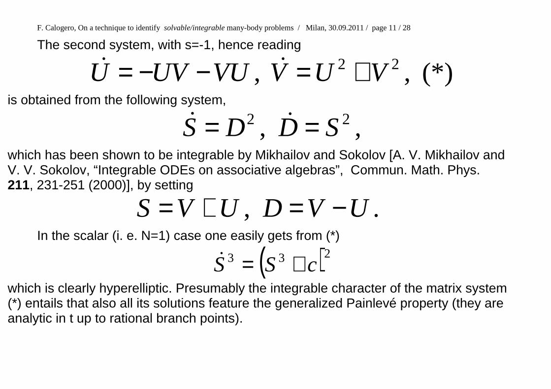
The second system, with s=-1, hence reading
(*),, 22 VUVVUUVU +=−−= &&
is obtained from the following system,
,, 22 SDDS == &&
which has been shown to be integrable by Mikhailov and Sokolov [A. V. Mikhailov and V. V. Sokolov, “Integrable ODEs on associative algebras”, Commun. Math. Phys. 211, 231-251 (2000)], by setting
., UVDUVS −=+=
In the scalar (i. e. N=1) case one easily gets from (*)
( )233 cSS +=&
which is clearly hyperelliptic. Presumably the integrable character of the matrix system (*) entails that also all its solutions feature the generalized Painlevé property (they are analytic in t up to rational branch points).
F. Calogero, On a technique to identify solvable/integrable many-body problems / Milan, 30.09.2011 / page 12 / 28
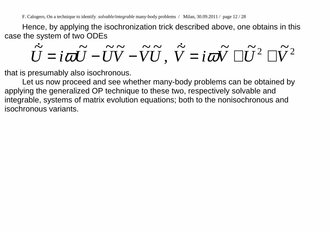
Hence, by applying the isochronization trick described above, one obtains in this case the system of two ODEs
22 ~~~~,
~~~~~~VUViVUVVUUiU ++=−−= ωω &&
that is presumably also isochronous. Let us now proceed and see whether many-body problems can be obtained by applying the generalized OP technique to these two, respectively solvable and integrable, systems of matrix evolution equations; both to the nonisochronous and isochronous variants.
F. Calogero, On a technique to identify solvable/integrable many-body problems / Milan, 30.09.2011 / page 13 / 28
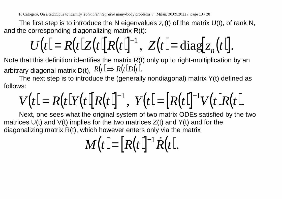
The first step is to introduce the N eigenvalues zn(t) of the matrix U(t), of rank N, and the corresponding diagonalizing matrix R(t):
( ) ( ) ( ) ( )[ ] ( ) ( )[ ].diag,1 tztZtRtZtRtU n== −
Note that this definition identifies the matrix R(t) only up to right-multiplication by an
arbitrary diagonal matrix D(t), ( ) ( ) ( ).tDtRtR ⇒ The next step is to introduce the (generally nondiagonal) matrix Y(t) defined as
follows:
( ) ( ) ( ) ( )[ ] ( ) ( )[ ] ( ) ( )., 11 tRtVtRtYtRtYtRtV −− == Next, one sees what the original system of two matrix ODEs satisfied by the two matrices U(t) and V(t) implies for the two matrices Z(t) and Y(t) and for the diagonalizing matrix R(t), which however enters only via the matrix
( ) ( )[ ] ( ).1 tRtRtM &−=
F. Calogero, On a technique to identify solvable/integrable many-body problems / Milan, 30.09.2011 / page 14 / 28
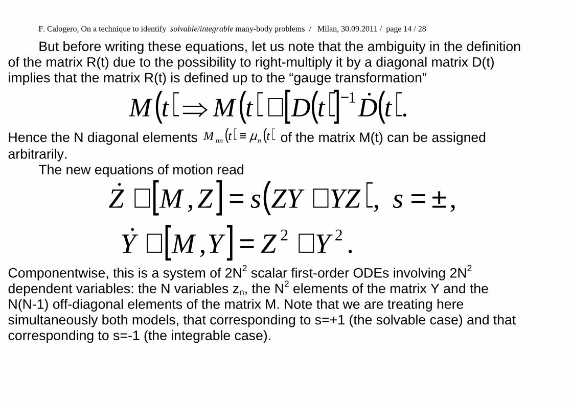
But before writing these equations, let us note that the ambiguity in the definition of the matrix R(t) due to the possibility to right-multiply it by a diagonal matrix D(t) implies that the matrix R(t) is defined up to the “gauge transformation”
( ) ( ) ( )[ ] ( ).1 tDtDtMtM &−+⇒ Hence the N diagonal elements ( ) ( )ttM nnn µ≡ of the matrix M(t) can be assigned arbitrarily.
The new equations of motion read
[ ] ( )[ ] .,
,,,22 YZYMY
sYZZYsZMZ
+=+±=+=+
&
&
Componentwise, this is a system of 2N2 scalar first-order ODEs involving 2N2 dependent variables: the N variables zn, the N2 elements of the matrix Y and the N(N-1) off-diagonal elements of the matrix M. Note that we are treating here simultaneously both models, that corresponding to s=+1 (the solvable case) and that corresponding to s=-1 (the integrable case).
F. Calogero, On a technique to identify solvable/integrable many-body problems / Milan, 30.09.2011 / page 15 / 28
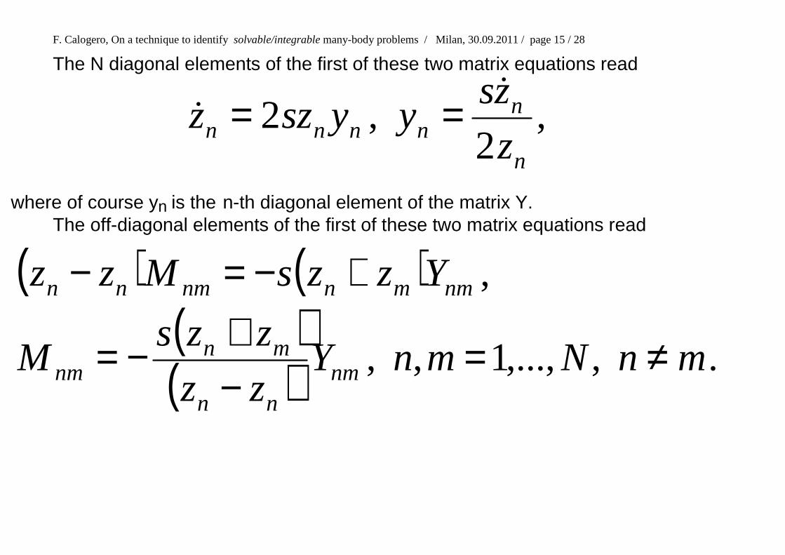
The N diagonal elements of the first of these two matrix equations read
,2
,2n
nnnnn z
zsyyszz
&& ==
where of course yn is the n-th diagonal element of the matrix Y. The off-diagonal elements of the first of these two matrix equations read ( ) ( )
( )( ) .,,...,1,,
,
mnNmnYzz
zzsM
YzzsMzz
nmnn
mnnm
nmmnnmnn
≠=−+−=
+−=−
F. Calogero, On a technique to identify solvable/integrable many-body problems / Milan, 30.09.2011 / page 16 / 28
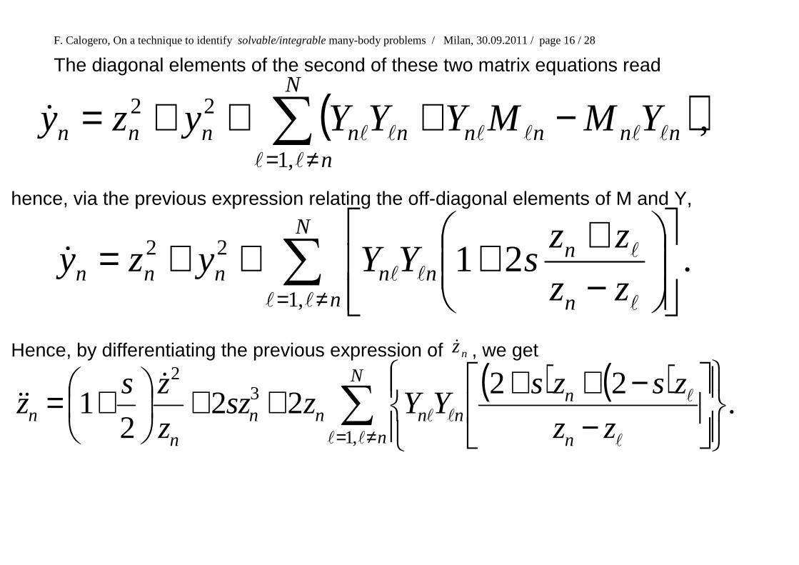
The diagonal elements of the second of these two matrix equations read
( ),,1
22 ∑≠=
−+++=N
nnnnnnnnnn YMMYYYyzy
ll
llllll&
hence, via the previous expression relating the off-diagonal elements of M and Y,
.21,1
22 ∑≠=
−++++=
N
n n
nnnnnn zz
zzsYYyzy
ll l
l
ll&
Hence, by differentiating the previous expression of nz& , we get
( ) ( ).
2222
21
,1
32
∑≠=
−−++++
+=N
n n
nnnnn
nn zz
zszsYYzsz
z
zsz
ll l
l
ll
&&&

F. Calogero, On a technique to identify solvable/integrable many-body problems / Milan, 30.09.2011 / page 17 / 28
Finally, the off-diagonal elements of the second of the two matrix equations read
( ) ( ),1 ,1∑ ∑
= ≠=
−+=N
k
N
nnnnnknnknm YMMYYYY
ll
llll
&
yielding, via the previous equations (and a bit of trivial algebra),
.;,...,1,
,11
221
21
,,1
mnNmn
zzzzszs
Y
YY
zz
zz
z
z
z
zs
Y
Y
N
mn mnnm
mn
mn
mn
m
m
n
nmn
nm
nm
≠=
−+
−+++
−−−
+
+++−=
∑≠= ll ll
l
ll
&&&&&
µµ
F. Calogero, On a technique to identify solvable/integrable many-body problems / Milan, 30.09.2011 / page 18 / 28
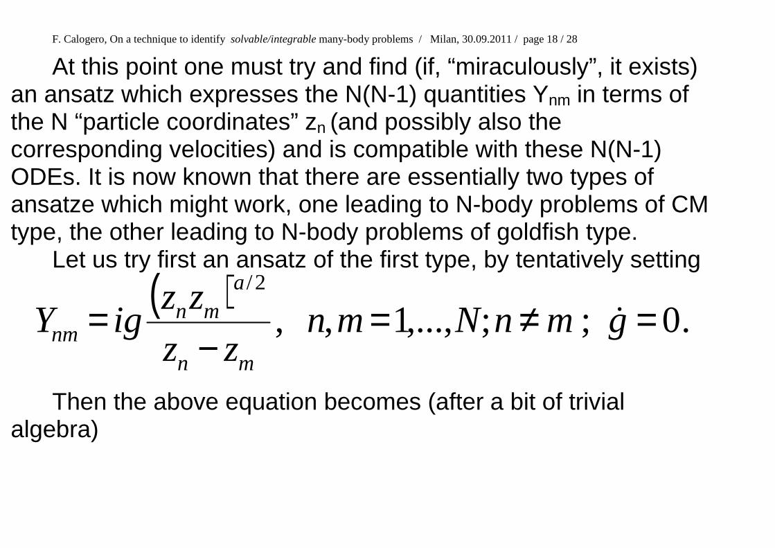
At this point one must try and find (if, “miraculously”, it exists) an ansatz which expresses the N(N-1) quantities Ynm in terms of the N “particle coordinates” zn (and possibly also the corresponding velocities) and is compatible with these N(N-1) ODEs. It is now known that there are essentially two types of ansatze which might work, one leading to N-body problems of CM type, the other leading to N-body problems of goldfish type.
Let us try first an ansatz of the first type, by tentatively setting
( ).0;;,...,1,,
2/
=≠=−
= gmnNmnzz
zzigY
mn
amn
nm &
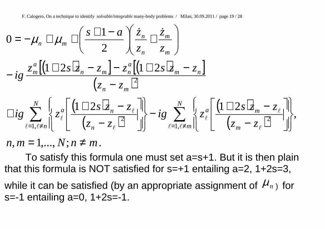
Then the above equation becomes (after a bit of trivial algebra)
F. Calogero, On a technique to identify solvable/integrable many-body problems / Milan, 30.09.2011 / page 19 / 28
( )[ ] ( )[ ]( )
( )( )
( )( )
.;,...,1,
,2121
2121
2
10
,12
,12
2
mnNmn
zz
zzszig
zz
zzszig
zz
zzszzzszig
z
z
z
zas
N
m m
maN
n n
na
mn
nmanmn
am
m
m
n
nmn
≠=
−−+−
−−++
−−+−−+−
+
−+++−=
∑∑≠=≠= ll l
l
l
ll l
l
l
&&µµ
To satisfy this formula one must set a=s+1. But it is then plain that this formula is NOT satisfied for s=+1 entailing a=2, 1+2s=3,
while it can be satisfied (by an appropriate assignment of nµ ) for s=-1 entailing a=0, 1+2s=-1.
F. Calogero, On a technique to identify solvable/integrable many-body problems / Milan, 30.09.2011 / page 20 / 28
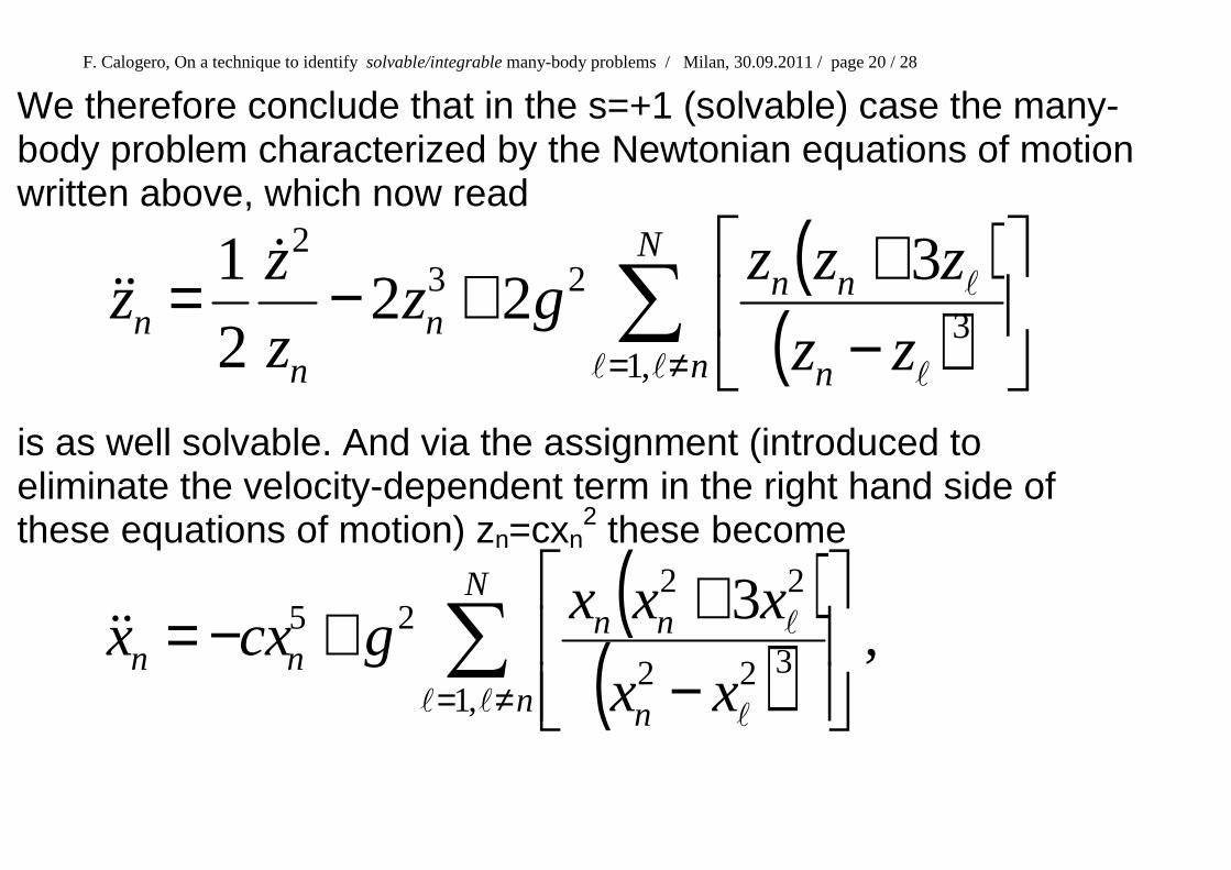
We therefore conclude that in the s=+1 (solvable) case the many-body problem characterized by the Newtonian equations of motion written above, which now read
( )( )∑
≠=
−++−=
N
n n
nnn
nn
zz
zzzgz
z
zz
ll l
l&
&&
,13
232 3
222
1
is as well solvable. And via the assignment (introduced to eliminate the velocity-dependent term in the right hand side of these equations of motion) zn=cxn
2 these become
( )( ) ,
3
,1322
2225 ∑
≠=
−++−=
N
n n
nnnn
xx
xxxgcxx
lll
l&&
F. Calogero, On a technique to identify solvable/integrable many-body problems / Milan, 30.09.2011 / page 21 / 28
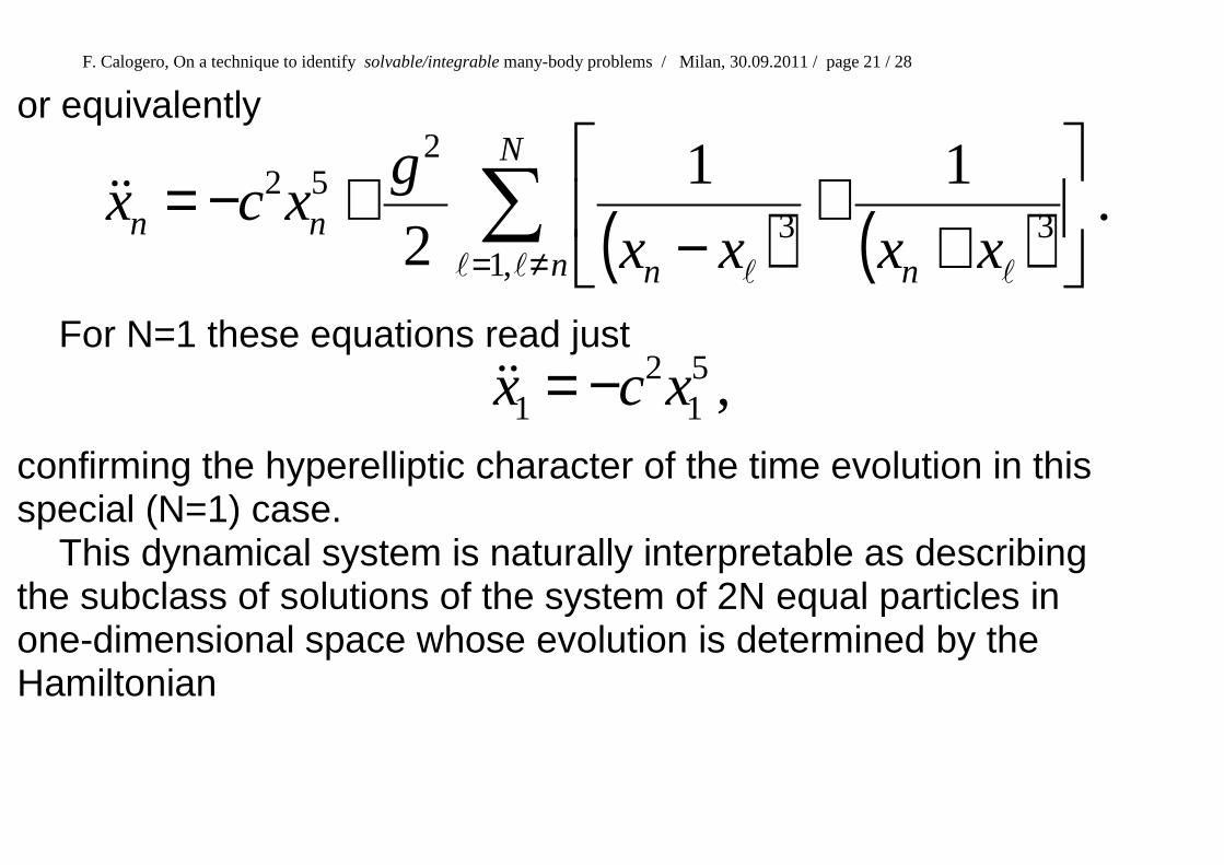
or equivalently
( ) ( ) .11
2 ,133
252 ∑
≠=
++
−+−=
N
n nn
nnxxxx
gxcx
ll ll
&&
For N=1 these equations read just
,51
21 xcx −=&&
confirming the hyperelliptic character of the time evolution in this special (N=1) case. This dynamical system is naturally interpretable as describing the subclass of solutions of the system of 2N equal particles in one-dimensional space whose evolution is determined by the Hamiltonian
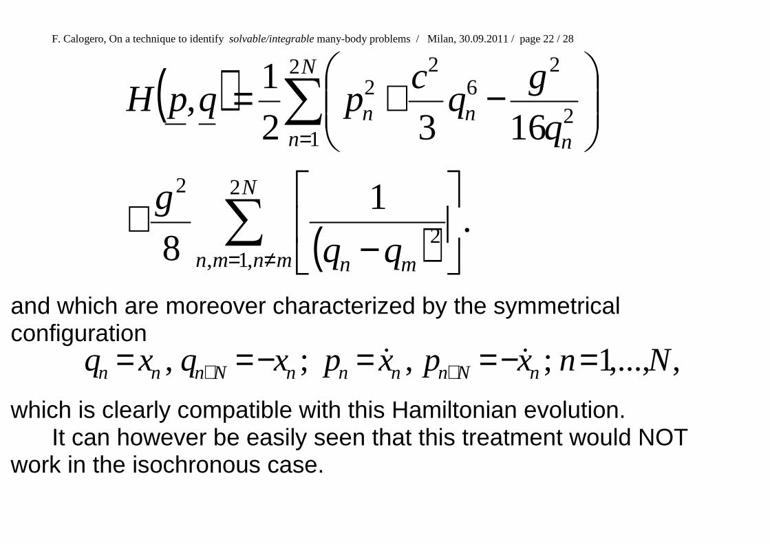
F. Calogero, On a technique to identify solvable/integrable many-body problems / Milan, 30.09.2011 / page 22 / 28
( )
( ) .1
8
16321
,
2
,1,2
2
2
12
26
22
∑
∑
≠=
=
−+
−+=
N
mnmn mn
N
n nnn
g
q
gq
cpqpH
and which are moreover characterized by the symmetrical configuration
,,...,1;,;, Nnxpxpxqxq nNnnnnNnnn =−==−== ++ &&
which is clearly compatible with this Hamiltonian evolution. It can however be easily seen that this treatment would NOT work in the isochronous case.
F. Calogero, On a technique to identify solvable/integrable many-body problems / Milan, 30.09.2011 / page 23 / 28
But let me emphasize that---contrary to what I thought until quite recently---the integrability of this system is NOT a new finding: indeed this system is a special case of a class of many-body problems whose integrability was demonstrated (by a different technique: Lax pairs and all that) long ago by V. I. Inozemtsev and D. V. Meshcheryakov, "Extension of the class of integrable dynamical systems connected with semisimple Lie algebras", Lett. Math. Phys. 9 (1985), 13-18.
Let us now try and see if the second ansatz (that generally leading to many-body models “of goldfish type”) might work. The following treatment shall be much more terse. I start by copying here again the relevant equations:
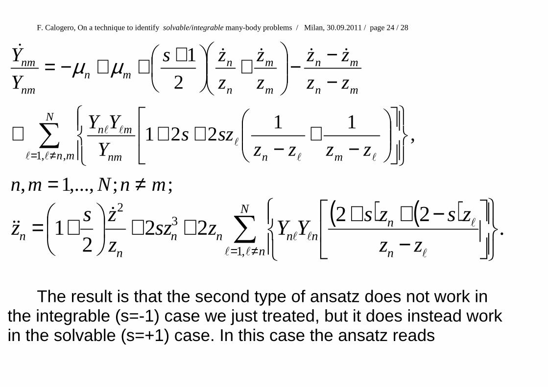
F. Calogero, On a technique to identify solvable/integrable many-body problems / Milan, 30.09.2011 / page 24 / 28
;;,...,1,
,11
221
21
,,1
mnNmn
zzzzszs
Y
YY
zz
zz
z
z
z
zs
Y
Y
N
mn mnnm
mn
mn
mn
m
m
n
nmn
nm
nm
≠=
−+
−+++
−−−
+
+++−=
∑≠= ll ll
l
ll
&&&&&
µµ
( ) ( ).
2222
21
,1
32
∑≠=
−−++++
+=N
n n
nnnnn
nn zz
zszsYYzsz
z
zsz
ll l
l
ll
&&&
The result is that the second type of ansatz does not work in the integrable (s=-1) case we just treated, but it does instead work in the solvable (s=+1) case. In this case the ansatz reads
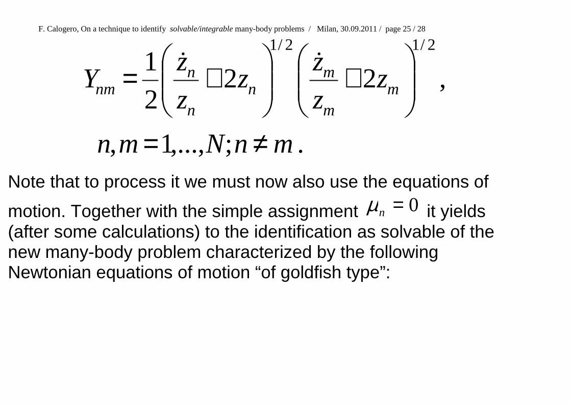
F. Calogero, On a technique to identify solvable/integrable many-body problems / Milan, 30.09.2011 / page 25 / 28
.;,...,1,
,2221
2/12/1
mnNmn
zz
zz
z
zY m
m
mn
n
nnm
≠=
+
+= &&
Note that to process it we must now also use the equations of
motion. Together with the simple assignment 0=nµ it yields (after some calculations) to the identification as solvable of the new many-body problem characterized by the following Newtonian equations of motion “of goldfish type”:
F. Calogero, On a technique to identify solvable/integrable many-body problems / Milan, 30.09.2011 / page 26 / 28
( )( )( )
.22
2
222
346
,1
22
1
23
∑
∑
≠=
=
−+++
+++−−=
N
n n
nn
N
kk
k
knnnnnn
zz
zzzz
zz
zzzzzzz
ll l
ll&&
&&&&&
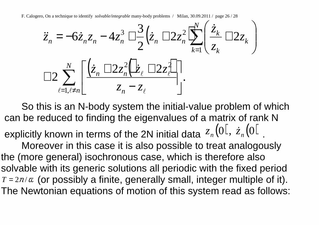
So this is an N-body system the initial-value problem of which can be reduced to finding the eigenvalues of a matrix of rank N
explicitly known in terms of the 2N initial data ( ) ( )0,0 nn zz & . Moreover in this case it is also possible to treat analogously the (more general) isochronous case, which is therefore also solvable with its generic solutions all periodic with the fixed period
ωπ /2=T (or possibly a finite, generally small, integer multiple of it). The Newtonian equations of motion of this system read as follows:

F. Calogero, On a technique to identify solvable/integrable many-body problems / Milan, 30.09.2011 / page 27 / 28
( ) ( )
( )( )( )
.22
2
222
3
42362
432
2
3
,1
22
1
2
322
∑
∑
≠=
=
−+−+−+
++−+
−−−−−−−−−=
N
n n
nnn
N
kk
k
knnn
nnnnnnn
zz
zzizzziz
zz
zzziz
zziNzzzN
ziNz
ll l
lll&&
&&
&&&
ωω
ω
ωωω
Other nontrivial solvable nonlinear dynamical systems obtain by looking at the time evolution of the N coefficients of monic polynomials of degree N whose N zeros are the N coordinates zn(t), or at the behaviour of these systems in the neighbourhood of their equilibria.
F. Calogero, On a technique to identify solvable/integrable many-body problems / Milan, 30.09.2011 / page 28 / 28
Mille Auguri
FRANCO
Buon Compleanno!!!


![CHEREDNIK ALGEBRAS AND CALOGERO-MOSER … · arxiv:1708.09764v2 [math.rt] 7 sep 2017 cÉdric bonnafÉ raphaËl rouquier cherednik algebras and calogero-moser cells](https://img.pdfslide.net/doc/110x75/5afa3f047f8b9a5f588f3309/cherednik-algebras-and-calogero-moser-170809764v2-mathrt-7-sep-2017-cdric.jpg)