F L Y A M T E - SRIJAN (सृजन) TUTORIALS · 3.4.2 Mobile-Controlled Handoff (Soft Handoff) 53 3.4.3 Handoff Prioritizing Schemes 55 3.5 Managing Resource Allocation 55 3.5.1

TEAMFLY

Team-Fly®

Location Management and Routing inMobile Wireless Networks

For a complete listing of the Artech House Mobile Communications Library,turn to the back of this book.

Location Management and Routing inMobile Wireless Networks

Amitava MukherjeeSomprakash Bandyopadhyay

Debashis Saha

Artech HouseBoston • London

www.artechhouse.com

Library of Congress Cataloging-in-Publication DataMukherjee, Amitava, 1959–

Location management and routing in mobile wireless networks / Amitava Mukherjee,Somprakash Bandyopadhyay, Debashis Saha.

p. cm. — (Artech House mobile communications series)Includes bibliographical references and index.ISBN 1-58053-355-8 (alk. paper)1. Wireless communication systems—Location. 2. Wireless communication systems—Management. 3. Routers (Computer networks) I. Bandyopadhyay, Somprakash, 1957–II. Saha, Debashis, 1965– III. Title. IV. Series.

TK5103.2.M85 2003621.382—dc21 2003041889

British Library Cataloguing in Publication DataMukherjee, Amitava, 1959–Location management and routing in mobile wireless networks. — (Artech House mobile com-munications series)

1. Mobile communication systems I. Title II. Bandyopadhyay, Somprakash, 1957–III. Saha, Debashis, 1965–

621 . 3’8456

ISBN 1-58053-355-8

Cover design by Yekaterina Ratner

© 2003 ARTECH HOUSE, INC.685 Canton StreetNorwood, MA 02062

All rights reserved. Printed and bound in the United States of America. No part of this bookmay be reproduced or utilized in any form or by any means, electronic or mechanical, includingphotocopying, recording, or by any information storage and retrieval system, without permissionin writing from the publisher.

All terms mentioned in this book that are known to be trademarks or service marks have beenappropriately capitalized. Artech House cannot attest to the accuracy of this information. Use ofa term in this book should not be regarded as affecting the validity of any trademark or servicemark.

International Standard Book Number: 1-58053-355-8Library of Congress Catalog Card Number: 2003041889

10 9 8 7 6 5 4 3 2 1

Contents

Preface xi

Acknowledgments xv

Part I: Cellular Networks

1 Introduction 1

1.1 Mobile Wireless Networks 5

1.2 Cellular Networks 6

1.2.1 Cellular Network Standards 7

1.2.2 Cellular Architecture 8

1.2.3 Medium Access 9

1.3 Ad Hoc Wireless Networks 10

1.4 Location Management 11

1.4.1 Location Updating and Paging 11

1.4.2 Mobility Models 12

1.4.3 Location Tracking 13

1.4.4 Radio Resource Management 13

1.5 Wireless Routing Techniques 13References 15

v

2 Mobility Issues 17

2.1 Introduction 17

2.2 Mobility Models 18

2.2.1 Fluid Flow Model 18

2.2.2 Diffusion Model 22

2.2.3 Gravity Model 22

2.2.4 Random Walk Model 23

2.3 Mobility in 3G Systems 26

2.3.1 Metropolitan Mobility 26

2.3.2 National Mobility Model 28

2.3.3 International Mobility Model 29References 29

3 Radio Resource Management 31

3.1 Radio Propagation 32

3.1.1 Path Loss 33

3.1.2 Shadowing Effects 35

3.1.3 Reciprocity 35

3.1.4 Indoor Wireless 37

3.2 Radio Resource (Spectrum Allocation) 37

3.2.1 Radio Frequency Spectrum Allocation 38

3.2.2 International Allocations 38

3.2.3 Financing for Spectrum Management 39

3.2.4 Spectrum Monitoring and Enforcement 39

3.2.5 GSM Frequencies 41

3.2.6 IMT-2000 (Third-Generation) Core Frequency Band 41

3.2.7 IMT-2000 (Third-Generation) Extension Bands 42

3.3 RRM 43

3.3.1 RRM Problem 43

3.3.2 Channel Allocation and Assignment 46

3.3.3 Schemes for CA 47

3.3.4 Transmitter Power Control 50

3.4 Handoff Process 52

3.4.1 Network-Controlled Handoff (Hard Handoff) 52

vi Location Management and Routing in Mobile Wireless Networks

3.4.2 Mobile-Controlled Handoff (Soft Handoff) 53

3.4.3 Handoff Prioritizing Schemes 55

3.5 Managing Resource Allocation 55

3.5.1 CAC 56

3.5.2 QoS 58

3.6 Emerging RRM Techniques 60

3.6.1 Cell Partitioning 60

3.6.2 Multilayered Architecture 61

3.6.3 Software Radio 61

3.7 Integrated RRM 63

3.8 Summary 65References 67

4 Location Management 69

4.1 Location Update 71

4.1.1 Location Update Static Strategies 72

4.1.2 Location Update Dynamic Strategies 72

4.2 Paging 75

4.2.1 Blanket Paging 75

4.2.2 Different Paging Procedures 77

4.3 Intelligent Paging Scheme 78

4.3.1 Sequential Intelligent Paging 81

4.3.2 PSIP 82

4.3.3 Comparison of Paging Costs 83

4.4 More Paging Schemes 84

4.4.1 Reverse Paging 85

4.4.2 Semireverse Paging 86

4.4.3 Uniform Paging 86

4.5 Intersystem Paging 87

4.6 IP Micromobility and Paging 88

4.7 Location Management 89

4.7.1 Without Location Management 90

4.7.2 Manual Registration in Location Management 90

Contents vii

4.7.3 Automatic Location Management Using LA 91

4.7.4 Memoryless-Based Location Management Methods 91

4.7.5 Memory-Based Location Management Methods 92

4.7.6 Location Management in Next-Generation Systems 93

4.8 LA Planning 97

4.8.1 Two-Step Approach 97

4.8.2 LA Planning and Signaling Requirements 107

4.9 Conclusion 109References 109

Part II: Ad Hoc Wireless Networks

5 Overview 117

5.1 Characteristics of Ad Hoc Networks 117

5.2 Three Fundamental Design Choices 118

5.2.1 Flat Versus Hierarchical Architecture 119

5.2.2 Proactive Versus Reactive Routing 120

5.2.3 Medium Access Protocol 121References 123

6 MAC Techniques in Ad Hoc Networks 125

6.1 MAC Protocols with Omnidirectional Antennas 125

6.2 MAC Protocols with Directional Antennas 128

6.3 Discussions 132References 133

7 Routing Protocols in Ad Hoc Wireless Networks 135

7.1 Introduction 135

7.2 Unicast Routing Protocols in Ad Hoc Networks 138

7.2.1 Proactive Routing Protocols 138

7.2.2 Reactive Routing Protocols 142

7.2.3 A Mobile Agent-Based Protocol for TopologyDiscovery and Routing 154

7.2.4 Power-Aware Routing Protocols in Ad Hoc Networks 158

viii Location Management and Routing in Mobile Wireless Networks

7.2.5 Other Routing Protocols 163

7.3 Multicast Routing Protocols in Ad Hoc Networks 165

7.4 Performance Comparisons of Unicast andMulticast Routing Protocols 168

7.4.1 Performance Comparisons ofMajor Unicast Routing Protocols 168

7.4.2 Performance Comparisons ofMajor Multicast Routing Protocols 170

7.5 Discussion 170References 172

Part III: Future Issues

8 Routing in Next-Generation Wireless Networks 179

8.1 UMTS All-IP Networks 179

8.2 Routing in Distributed Wireless Sensor Networks 182

8.2.1 Introduction 182

8.2.2 Sensor Networks 182

8.2.3 Topology Maintenance and Sensor Deployment 183

8.2.4 Routing 184

8.3 Pervasive Routing 186References 189

9 Conclusion 191

List of Acronyms 195

About the Authors 203

Index 205

Contents ix

.

TEAMFLY

Team-Fly®

Preface

This book aims at presenting, in a canonical form, the work done by us in thefield of routing in mobile wireless networks. Most of the material containedherein has previously been presented at international conferences or has beenaccepted for publication in journals.

Mobile wireless networks can be broadly classified into two distinct cate-gories: infrastructured (cellular) and infrastructureless (ad hoc). While cellularnetworks usually involve a single-hop wireless link to reach a mobile terminal,ad hoc networks normally require a multihop wireless path from a source to adestination. The growth of mobility aspects in cellular networks is occurring atthree different levels. First, growth occurs at the spatial level (i.e., users desire toroam with a mobile terminal). Second, growth occurs from the penetration rateof mobile radio access lines. And third, the traffic generated by each wireless useris constantly growing. On one hand, tetherless (e.g., cellular) subscribers usetheir mobile terminals; on the other hand, the arrival of more capacity-greedyservices (e.g., Internet accesses, multimedia services). From all of these consid-erations, the generalized mobility features will have serious impacts on the wire-less telecommunications networks. Mobility can be categorized into two areas:radio mobility, which mainly consists of the handover process and networkmobility, which mainly consists of location management (location updating andpaging). In this book, we shall concentrate on the network mobility only.

This book will act as a general introduction to location management,and routing in both single-hop and multihop mobile wireless networks, so thatreaders can gain familiarity with location management and routing issues inthis field. In particular, it will provide the details of location management andpaging in wireless cellular networks, and routing in mobile ad hoc networks.

xi

In about 200 pages, it will cover the past, present, and future works on loca-tion management and routing protocols in all types of mobile wireless networks.In cellular networks, the emphasis will be on mobility issues, location manage-ment, paging, and radio resources. In mobile ad hoc networks, the focus will beon different types of routing protocols and medium access control techniques.It will discuss numerous potential applications, review relevant concepts, andexamine the various approaches that enable readers to understand the issues andfuture research problems in this field too. In a word, it will cover everything youcan think in the realm of location management and routing issues in mobilewireless networks.

Barring Chapter 1, which is a general introduction to the subject, the bookis divided into three parts, namely Part I: Cellular Networks, Part II: Ad HocWireless Networks, and Part III: Future Issues. In Part I, there are three chap-ters. Chapter 2 concentrates on two important mobility issues, namely mobilitymodels (fluid-flow model, random walk model, gravity model), and mobilitytraces (metropolitan mobility, national mobility, international mobility). Chap-ter 3 concerns radio resource management, including radio propagation, andchannel assignment. Chapter 4 describes an important issue called locationmanagement. It covers issues such as paging (blanket paging, and intelligentpaging), location update (static location update, dynamic location update) andlocation area planning (manual registration, automatic location managementusing location area, memory-based location management methods, non-memory-based location methods, location management in CDPD, GPRS,WCDMA, and IMT-2000).

Part II focuses on ad hoc wireless networks and again comprises threechapters. Chapter 5 is an overview of the characteristics of ad hoc networksincluding three fundamental design choices, namely flat versus hierarchicalarchitecture, proactive versus reactive routing, and medium access protocols.Chapter 6 describes medium access control techniques in detail, covering basicmedia access protocol for wireless LANs (IEEE 802.11), Floor Acquisition Mul-tiple Access, Dual Busy Tone Multiple Access, Power Controlled MultipleAccess Protocols, MAC with Adaptive Antenna, Directional MAC Protocols,and Adaptive MAC Protocol for WACNet. Chapter 7 discusses both unicastand multicast routing protocols in ad hoc wireless networks. Unicast routingtechniques include proactive routing protocols, such as DSDV, WRP, CBR,CGSR, OLSR, FSR, and agent-based protocols for topology discovery and rout-ing, and reactive routing protocols, such as DSR, AODV, TORA,ABR, SSA, stability-based routing, LAR, and query localization techniques foron-demand routing. It also includes power-aware routing, multipath routing,and QoS Management.

xii Location Management and Routing in Mobile Wireless Networks

Part III explores future issues such as routing in next-generation wirelessnetworks, location management in all-IP IMT-2000 networks, routing in adhoc sensor networks, and routing in pervasive networks.

This book is a uniquely comprehensive study of the major location man-agement and routing technologies and systems that will assist in forming thefuture mobile wireless networks. We have written the book for those profession-als and students who want such a comprehensive view. It may be used as a textor reference book in graduate courses in mobile wireless networks.

Preface xiii

.

Acknowledgments

We want to express our sincere gratitude towards Artech House Books for giv-ing us the opportunity to write on this topic. Many thanks also to our colleaguesat the department, past and present, for many rewarding discussions and forcontributing to the stimulating and pleasant atmosphere.

Several other people helped us during the course of writing this book. Wewould like to specially thank our colleagues at Indian Institute of Management(IIM), Calcutta and i-SDC SBU, IBM Global Services, Calcutta. Special thanksgo to Amitabh Ray, Agnimitra Biswas, Surojit Mookherjee and Reena J. Sarkarof IBM Global Services, Calcutta and Jaydeep Mukherjee of Cogentech Man-agement Consultants (P) Ltd., Calcutta.

The main bulk of the work was carried out by our doctoral students,namely Partha Sarathi Bhattacharjee of Bharat Sanchar Nigam Ltd., Calcuttaand Krishna Paul of Indian Institute of Technology, Bombay. We express ourgratitude to them. Many thanks to Sauti Sen for designing the cover layout.

It is with pleasure that we also acknowledge and thank the editorial staffof Artech House Books. Tiina Ruonamaa, assistant editor, and Dr. Julie Lanca-shire, senior commissioning editor, Artech House Books, have helped withlogistics and with their enthusiasm in giving the prompt reminders beforethe promised deadlines. Finally, our thanks go to the production department ofArtech House Books for managing with a very tight schedule.

Last but not least, we want to thank our families for their support andencouragement throughout this time.

xv

.

Part ICellular Networks

.

1Introduction

Wireless communication has recently captured the attention and the imagina-tion of users from all walks of life. The major goal of wireless communication isnow to allow a user to have access to the capabilities of global networks at anytime without regard to location or mobility. Since their emergence in the 1970s[1], the mobile wireless networks have become increasingly popular in the net-working industry. This has been particularly true within the past decade, whichhas seen wireless networks being adapted to enable mobility. Since the inceptionof cellular telephones in the early 1980s [2], they have evolved from a costlyservice with limited availability toward an affordable and more versatile alterna-tive to wired telephony. In the future, it appears that, not only will cellularinstallations continue to proliferate, but wireless access to fixed telephones willbecome much more common.

Trends in wireless communication are proceeding with a strong ten-dency toward increasing need for mobility in the access links within the net-work. Examples are (1) residential line access with the proliferation ofcordless phones and their penetration rate having passed that of fixed phones inseveral countries including the United States and Japan; (2) business lines withwireless private branch exchange (WPBX) access for voice services, and wire-less LANs (WLANs) for computer-oriented data communications such as IEEE802.11 and HIPERLAN specifications; and (3) cellular systems, which allowtelecommunication and limited data accesses over wide areas [3]. Observingthese trends, it can be predicted that the traffic over next-generation high-speed wireless networks will be dominated by personal multimedia applica-tions such as fairly high-speed data, video, and multimedia traffic. This genera-tion is known as third-generation system (see Table 1.1). From this viewpoint,

1

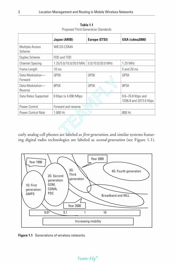
early analog cell phones are labeled as first-generation, and similar systems featur-ing digital radio technologies are labeled as second-generation (see Figure 1.1).

2 Location Management and Routing in Mobile Wireless Networks

Table 1.1Proposed Third-Generation Standards

Japan (ARIB) Europe (ETSI) USA (cdma2000)

Multiple AccessScheme

WB DS-CDMA

Duplex Scheme FDD and TDD

Channel Spacing 1.25/5.0/10.0/20.0 MHz 5.0/10.0/20.0 MHz 1.25 MHz

Frame Length 10 ms 5 and 20 ms

Data Modulation—Forward

QPSK QPSK QPSK

Data Modulation—Reverse

BPSK QPSK BPSK

Data Rates Supported 8 Kbps to 4.096 Mbps 9.6–76.8 Kbps and1036.8 and 2073.6 Kbps

Power Control Forward and reverse

Power Control Rate 1,600 Hz 800 Hz

Broadband and WLL

4G: Fourth generation3G:Thirdgeneration

2G: Secondgeneration:GSM,CDMA,PDC

1G: Firstgeneration:AMPS

Year 2005

Year 2000

0.01 0.1 1 10

Increasing mobility

Year 1990

Figure 1.1 Generations of wireless networks.

TEAMFLY

Team-Fly®

The principal advantages of second-generation (digital) systems over their first-generation (analog) predecessors are greater capacity and less frequent need forbattery charging [1, 2]. In other words, they accommodate more users in a givenpiece of spectrum and they consume less power. Second generation networks,however, retain the circuit-switching legacy of analog networks. They were alloriginally designed to carry voice traffic, which has little tolerance for delay jit-ter. Data services are more tolerant of network latencies.

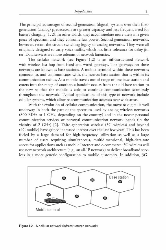
The cellular network (see Figure 1.2) is an infrastructured networkwith wireless last hop from fixed and wired gateways. The gateways for thesenetworks are known as base stations. A mobile terminal within these networksconnects to, and communicates with, the nearest base station that is within itscommunication radius. As a mobile travels out of range of one base station andenters into the range of another, a handoff occurs from the old base station tothe new so that the mobile is able to continue communication seamlesslythroughout the network. Typical applications of this type of network includecellular systems, which allow telecommunication accesses over wide areas.

With the evolution of cellular communication, the move to digital is wellunderway in both the part of the spectrum used by analog wireless networks(800 MHz to 1 GHz, depending on the country) and in the newer personalcommunication services or personal communication network bands (in thevicinity of 2 GHz) [2]. Third-generation wireless (3G wireless) and beyond(4G mobile) have gained increased interest over the last few years. This has beenfueled by a large demand for high-frequency utilization as well as a largenumber of users requiring simultaneous, multidimensional, high-data-rateaccess for applications such as mobile Internet and e-commerce. 3G wireless willuse new network architecture (e.g., an all-IP network) to deliver broadband serv-ices in a more generic configuration to mobile customers. In addition, 3G

Introduction 3

Base station

Mobile terminal

Figure 1.2 A cellular network (infrastructured network).

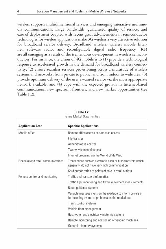
wireless supports multidimensional services and emerging interactive multime-dia communications. Large bandwidth, guaranteed quality of service, andease of deployment coupled with recent great advancements in semiconductortechnologies for wireless applications make 3G wireless a very attractive solutionfor broadband service delivery. Broadband wireless, wireless mobile Inter-net, software radio, and reconfigurable digital radio frequency (RF)are all emerging as a result of the tremendous development in wireless semicon-ductors. For instance, the vision of 4G mobile is to (1) provide a technologicalresponse to accelerated growth in the demand for broadband wireless connec-tivity; (2) ensure seamless services provisioning across a multitude of wirelesssystems and networks, from private to public, and from indoor to wide area; (3)provide optimum delivery of the user’s wanted service via the most appropriatenetwork available; and (4) cope with the expected growth in Internet-basedcommunications, new spectrum frontiers, and new market opportunities (seeTable 1.2).


Table 1.2Future Market Opportunities

Application Area Specific Applications

Mobile office Remote office access or database access

File transfer

Administrative control

Two-way communications

Internet browsing via the World Wide Web

Financial and retail communications Transactions such as electronic cash or fund transfers which,generally, do not have very high communication

Card authorization at points of sale in retail outlets

Remote control and monitoring Traffic and transport informatics

Traffic light monitoring and traffic movement measurements

Route guidance systems

Variable message signs on the roadside to inform drivers offorthcoming events or problems on the road ahead

Trains control systems

Vehicle fleet management

Gas, water and electrically metering systems

Remote monitoring and controlling of vending machines

General telemetry systems

1.1 Mobile Wireless Networks

Wireless networks are of two types: fixed and mobile. Fixed wireless networksdo not support mobility and are mostly point-to-point (e.g., microwave net-works, geostationary satellite networks). On the other hand, mobile wireless net-works are more versatile as they allow user mobility. Mobile wireless networksare, again, broadly classified into two distinct categories: infrastructured (cellu-lar) and infrastructureless (ad hoc). Both aim to create a ubiquitous communica-tion as well as computing environment where users are untethered from theirinformation sources, that is, they get “anytime, anywhere access to information,communication, and service” with the help of the wireless mobile technolo-gies.While cellular networks usually involve a single-hop (access only) wirelesslink to reach a mobile terminal, ad hoc networks normally require a multihopwireless path from a source to a destination.

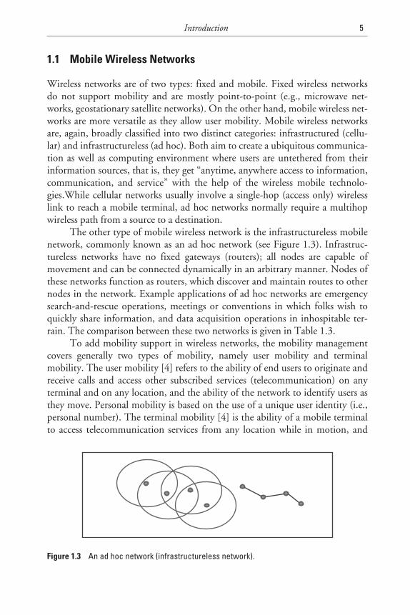
The other type of mobile wireless network is the infrastructureless mobilenetwork, commonly known as an ad hoc network (see Figure 1.3). Infrastruc-tureless networks have no fixed gateways (routers); all nodes are capable ofmovement and can be connected dynamically in an arbitrary manner. Nodes ofthese networks function as routers, which discover and maintain routes to othernodes in the network. Example applications of ad hoc networks are emergencysearch-and-rescue operations, meetings or conventions in which folks wish toquickly share information, and data acquisition operations in inhospitable ter-rain. The comparison between these two networks is given in Table 1.3.

To add mobility support in wireless networks, the mobility managementcovers generally two types of mobility, namely user mobility and terminalmobility. The user mobility [4] refers to the ability of end users to originate andreceive calls and access other subscribed services (telecommunication) on anyterminal and on any location, and the ability of the network to identify users asthey move. Personal mobility is based on the use of a unique user identity (i.e.,personal number). The terminal mobility [4] is the ability of a mobile terminalto access telecommunication services from any location while in motion, and

Introduction 5

Figure 1.3 An ad hoc network (infrastructureless network).

the capability of the network to locate and identify the mobile terminal as itmoves. Terminal mobility is associated with wireless access and requires the userto carry a terminal and be within the area of radio coverage.

1.2 Cellular Networks

Recent advances [1–3] in cellular communication have led to an unprecedentedgrowth of a collection of wireless communication systems that support both per-sonal and terminal mobility. This wide acceptance of cellular communicationhas led to the development of a new generation of mobile communication net-work, which can support a larger mobile subscriber population while providingvarious types of services unavailable to traditional cellular systems. Servicesinclude location independent universal phone numbering, future public landmobile telecommunications services (FPLMTS), WPBX, WLANs, telepointphone service, and satellite communications. It is envisaged that InternationalMobile Telecommunications 2000 (IMT-2000) networks (previously known asFPLMTS) will evolve from the existing wireless and fixed networks by addingnecessary capabilities for supporting IMT-2000 services. In a sense, IMT-2000systems are third-generation mobile communication systems designed to pro-vide global operation, an enhanced set of service capabilities, and significantlyimproved performance. While the first round of transition from analog (firstgeneration) to digital (second generation) was designed to fix the problems(such as security, blocking, and regional incompatibilities) in the analog sys-tems, the migration to the third generation is designed to open up a vista ofentirely new services. In this generation, it is estimated that the introduction ofdifferent types of services and the establishment of new service providers willresult in an unprecedented growth in the number of mobile subscribers from 15million currently to around 60 million by 2005.


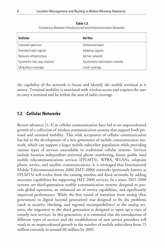
Table 1.3Comparison Between Infrastructured and Infrastructureless Networks

Cellular Ad Hoc

Licensed spectrum Unlicensed band

Standard radio signals Adaptive signals

Network infrastructure Ad hoc network

Symmetric two-way channel Asymmetric information transfer

Ubiquitous coverage Local coverage

1.2.1 Cellular Network Standards

Several wireless communications systems have achieved rapid growth due toheavy market demand. Obvious examples [2] include high-tier digital cellularsystems like Global System for Mobile Communication (GSM), AmericanDigital Cellular (ADC) or IS-54, Personal Digital Cellular (PDC), and DigitalCommunication System at 1,800 MHz (DCS1800) for widespread vehicularand pedestrian services, and low-tier cordless telecommunication systems basedon Cordless Telephone 2 (CT2), Digital European Cordless Telephone(DECT), Personal Access Communications Systems (PACS), and PersonalHandy Phone System (PHS) standards for residential, business, and publiccordless access applications. Although the design guidelines of such systems arequite different, their individual success may suggest a potential path to achievinga complete Personal Communications Systems (PCS) vision: integration of dif-ferent PCS systems, which is referred to as “heterogeneous PCS” (HPCS). Agood example of the migration from second-generation mobile systems (e.g.,GSM, IS-54) to the IMT-2000 vision is the evolution from the European Tele-communication Standardization Institute (ETSI)–defined GSM system to uni-versal mobile telecommunication systems (UMTS). The UMTS system is onlyone of the many new third-generation systems being developed around theworld, and serves as an illustration for our current discussion. UMTS cannot bedeveloped as a completely isolated network with minimal interface and serviceinterconnection to existing networks. Both UMTS and existing networks willneed to develop along parallel, even convergent paths, if service transparency isto be achieved to any degree. This would, in the end, allow UMTS service to besupported, although at different levels of functionality, across all networks.Another important requirement for seamless operation of the two standards isGSM-UMTS handover in both directions.

UMTS wideband code division multiple access (WCDMA) is one of themajor new third-generation mobile communication systems being developedwithin the IMT-2000 framework. It represents a substantial advance over exist-ing mobile communications systems. Additionally, it is being designed withflexibility for users, network operators, and service developers in mind andembodies many new and different concepts and technologies. UMTS servicesare based on standardized service capabilities, which are common throughout allUMTS users and radio environments. This means that personal users will expe-rience a consistent set of services even when they roam from their home networkto other UMTS operators—a virtual home environment (VHE). Users willalways feel that they are connected to their home network, even when roaming.VHEs will ensure the delivery of the service provider’s total environment (e.g., acorporate user’s virtual work environment), independent of the user’s locationor the mode of access. The ultimate goal is transparency (i.e., that all networks,signaling, connections, registrations, and any other technologies should be

Introduction 7

invisible to the user), ensuring that mobile multimedia services are simple, user-friendly, and effective.

1.2.2 Cellular Architecture

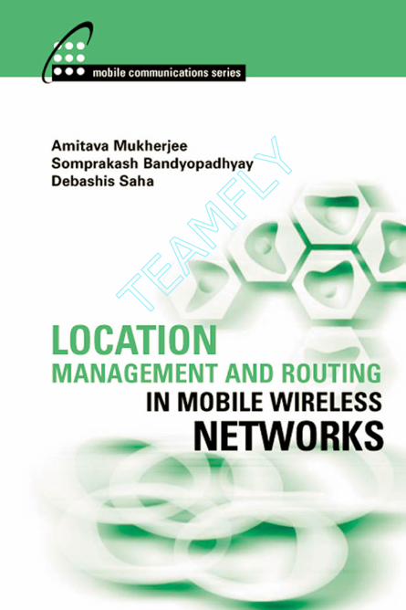
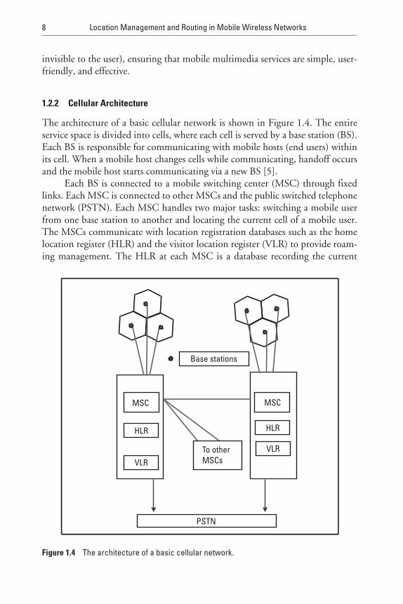
The architecture of a basic cellular network is shown in Figure 1.4. The entireservice space is divided into cells, where each cell is served by a base station (BS).Each BS is responsible for communicating with mobile hosts (end users) withinits cell. When a mobile host changes cells while communicating, handoff occursand the mobile host starts communicating via a new BS [5].

Each BS is connected to a mobile switching center (MSC) through fixedlinks. Each MSC is connected to other MSCs and the public switched telephonenetwork (PSTN). Each MSC handles two major tasks: switching a mobile userfrom one base station to another and locating the current cell of a mobile user.The MSCs communicate with location registration databases such as the homelocation register (HLR) and the visitor location register (VLR) to provide roam-ing management. The HLR at each MSC is a database recording the current


PSTN

MSC MSC

To otherMSCs

HLR

VLR

Base stations

HLR

VLR

Figure 1.4 The architecture of a basic cellular network.

location of each mobile that belongs to the MSC. And the VLR at each MSC isa database recording the cell of visiting mobiles.

The distinguishing feature of cellular systems compared to previousmobile radio systems is the use of many BSs with relatively small coverage radii(on the order of 10 km or less versus 50 to 100 km for earlier mobile systems).Multiple BSs, which are a few cells apart (e.g., 5 cells, 7 cells), use the same set offrequencies simultaneously. This frequency reuse allows a much higher sub-scriber density per megahertz of spectrum than earlier noncellular systems. Sys-tem capacity can be further increased by reducing the cell size (the coverage areaof a single BS) down to an area with a radius as small as 0.5 km. In addition tosupporting much higher subscriber densities than previous systems, thisapproach makes possible the use of small, battery-powered portable handsetswith lower RF transmit power than the large, vehicular mobile units used in ear-lier systems. In cellular systems, continuous coverage is achieved by executing ahandoff as the mobile unit crosses cell boundaries. This requires the mobile tochange frequencies under control of the cellular network.

1.2.3 Medium Access

The development of low-rate digital speech coding techniques and the continu-ous increase in the device density of integrated circuits (i.e., transistors per unitarea), have made completely digital second-generation systems viable. Secondgeneration cellular systems based on digital transmissions are currently beingused. Digitization allows the use of time division multiple access (TDMA) andcode division multiple access (CDMA) as alternatives to frequency division mul-tiple access (FDMA). With TDMA, the usage of each radio channel is parti-tioned into multiple timeslots, and each user is assigned a specific frequency andtimeslot combination. Thus, only a single mobile in a given cell is using a givenfrequency at any particular time. With CDMA, multiple mobiles in a given celluse a frequency channel simultaneously, and the signals are distinguished byspreading them with different codes. One obvious advantage of both TDMAand CDMA is the sharing of radio hardware in the BS among multiple users.Digital systems can support more users per BS per megahertz of spectrum,allowing wireless system operators to provide service in high-density areas moreeconomically. The use of TDMA or CDMA digital architectures also offersadditional advantages, including the following:

• A more natural integration with the evolving digital wireline network;

• Flexibility for mixed voice and data communication, and the support ofnew services;

• A potential for further capacity increases as reduced-rate speech codersare introduced;

Introduction 9

• Reduced RF transmit power (increasing battery life in handsets);

• Encryption for communication privacy;

• Reduced system complexity (e.g., mobile-assisted handoffs, fewer radiotransceivers).

1.3 Ad Hoc Wireless Networks

Most of the wireless mobile computing applications today require single hopwireless connectivity to the wired network. This is the traditional cellular net-work model, which supports the current mobile computing needs by installingBSs and access points. In such networks, communications between two mobilehosts completely rely on the wired backbone and the fixed BSs. A mobile host isonly one hop away from a BS.

At times, however, no wired backbone infrastructure may be available foruse by a group of mobile hosts. Also, there might be situations in which settingup fixed access points is not a viable solution due to cost, convenience, and per-formance considerations. Still, the group of mobile users may need to commu-nicate with each other and share information between them. In such situations,an ad hoc network can be formed. An ad hoc network is a temporary network,operating without the aid of any established infrastructure of centralizedadministration or standard support services regularly available on the wide areanetwork to which the hosts may normally be connected [6]. Applications of adhoc networks include military tactical communication, emergency relief opera-tions, and commercial and educational use in, for example, remote areas ormeetings where the networking is mission-oriented or community-based.

Ad hoc networks [6, 7] are envisioned as infrastructureless networks whereeach node is a mobile router equipped with a wireless transceiver. A messagetransfer in an ad hoc network environment would take place either between twonodes that are within the transmission range of each other or between nodes thatare indirectly connected via multiple hops through some other intermediatenodes. This is shown in Figure 1.5. Node C and node F are outside the wirelesstransmission range of each other but are still able to communicate via the inter-mediate node D in multiple hops.

There has been a growing interest in ad hoc networks in recent years[8, 9]. The basic assumption in an ad hoc network is that two nodes willing tocommunicate may be outside the wireless transmission range of each other, butthey are still able to communicate if other nodes in the network are willing andcapable of forwarding packets from them. The successful operation of an ad hocnetwork will be interrupted, however, if an intermediate node, participating in acommunication between two nodes, either moves out of range suddenly orswitches itself off in between message transfers. The situation is worse if there is


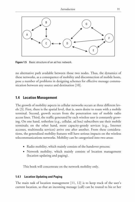
no alternative path available between those two nodes. Thus, the dynamics ofthese networks, as a consequence of mobility and disconnection of mobile hosts,pose a number of problems in designing schemes for effective message commu-nication between any source and destination [10].

1.4 Location Management

The growth of mobility aspects in cellular networks occurs at three different lev-els [3]. First, there is the spatial level, that is, users desire to roam with a mobileterminal. Second, growth occurs from the penetration rate of mobile radioaccess lines. Third, the traffic generated by each wireless user is constantly grow-ing. On one hand, tetherless (e.g., cellular, ad hoc) subscribers use their mobileterminals; on the other hand, more capacity-greedy services (e.g., Internetaccesses, multimedia services) arrive one after another. From these considera-tions, the generalized mobility features will have serious impacts on the wirelesstelecommunications networks. Mobility can be categorized into two areas:

• Radio mobility, which mainly consists of the handover process;

• Network mobility, which mainly consists of location management(location updating and paging).

This book will concentrate on the network mobility only.

1.4.1 Location Updating and Paging

The main task of location management [11, 12] is to keep track of the user’scurrent location, so that an incoming message (call) can be routed to his or her

Introduction 11

A

C

G

F

E

D

B

Figure 1.5 Basic structure of an ad hoc network.

mobile station (MS). Location management schemes are essentially based onusers’ mobility and incoming call rate characteristics. The network mobilityprocess has to face strong antagonism between its two basic procedures: (1)updating (or registration), the process by which a mobile endpoint initiates achange in the location database according to its new location; and (2) finding(or paging), the process by which the network initiates a query for an endpoint’slocation (which may also result in an update to the location database). The loca-tion updating procedure allows the system to keep the user’s location knowl-edge, more or less accurately, in order to be able to find him or her, in case of anincoming call, for example. Location updating is also used to bring the user’sservice profile near its location and allows the network to rapidly provide theuser with his or her services. The paging process achieved by the system consistsof sending paging messages in all cells where the mobile terminal could belocated.

Most location management techniques use a combination of updating andfinding in an effort to select the best trade-off between update overhead anddelay incurred in finding. Specifically, updates are not usually sent every time anendpoint enters a new cell, but rather are sent according to a predefined strategysuch that the finding operation can be restricted to a specific area. There is also atrade-off, analyzed formally, between the update and paging costs. For this pur-pose, the MS frequently sends location update messages to its current MSC. Ifthe MS seldom sends updates, its location (e.g., its current cell) is not knownexactly and paging is necessary for each downlink packet, resulting in a signifi-cant delivery delay. On the other hand, if location updates happen very often,the MS’s location is well known to the network, and the data packets can bedelivered without any additional paging delay. Quite a lot of uplink radio capac-ity and battery power, however, is consumed for mobility management in thiscase. Thus, a good location management strategy must be a compromisebetween these two extreme methods.

1.4.2 Mobility Models

Three mobility models, namely, the fluid flow model, the random-walk model,and the gravity model, are addressed [13]. The fluid flow model considers trafficflow as the flow of a fluid, modeling macroscopic movement behavior. Therandom-walk model (also known as Markovian model) describes individualmovement behavior in any cellular network. The gravity model has also beenused to model human movement behavior. It is also applied to regions of vary-ing sizes, from city mobility models to national and international mobility mod-els. Mobility traces indicate current movement behavior of users and are morerealistic than mobility models. However, mobility traces for large populationsizes and large geographical areas have been categorized into a hierarchy by three


TEAMFLY

Team-Fly®

different scales: Metropolitan Mobility Model, National Mobility Model, andInternational Mobility Model.

1.4.3 Location Tracking

In a cellular network, location-tracking mechanisms may be perceived as updat-ing and querying a distributed database (the location database) of endpointidentifier-to-address mappings [12]. In this context, location tracking has twocomponents: (1) determining when and how a change in a location databaseentry should be initiated, and (2) organizing and maintaining the location data-base. In cellular networks, endpoint mobility within a cell is transparent to thenetwork, and hence location tracking is only required when an endpoint movesfrom one cell to another. The location-tracking methods are broadly classifiedinto two groups. The first group includes all methods based on algorithms andnetwork architecture, mainly on the processing capabilities of the system. Thesecond group contains the methods based on learning processes, which requirethe collection of statistics on subscribers’ mobility behavior, for instance. Thistype of method emphasizes the information capabilities of the network.

1.4.4 Radio Resource Management

The problem of radio resource management is one important issue for good net-work performance. The radio resource management problem depends on thethree key allocation decisions that are concerned with waveforms (channels),access ports (or base stations), and with the transmitter powers. Both channelderivation and allocation methods will influence the performance. The use ofTDMA and CDMA are alternatives to FDMA used in the first-generation sys-tems. With TDMA, the usage of each radio channel is partitioned into multipletimeslots, and each user is assigned a specific frequency and timeslot combina-tion. Thus, only a single mobile in a given cell is using a given frequency at anyparticular time. With CDMA (which uses direct sequence spreading), multiplemobiles in a given cell use a frequency channel simultaneously, and the signalsare distinguished by spreading them with different codes. The channel alloca-tion is an essential feature in cellular networks and impacts the networkperformance.

1.5 Wireless Routing Techniques

A network must retain information about the locations of endpoints in the net-work, in order to route traffic to the correct destinations. Location tracking (alsoreferred to as mobility tracking or mobility management) is the set of mecha-nisms by which location information is updated in response to endpoint

Introduction 13

mobility. In location tracking, it is important to differentiate between the iden-tifier of an endpoint (i.e., what the endpoint is called) and its address (i.e., wherethe endpoint is located). Mechanisms for location tracking provide a time vary-ing mapping between the identifier and the address of each endpoint [12].

In any communication network, procedures for route selection and trafficforwarding require accurate information about the current state of the network(e.g., node interconnectivity, link quality, traffic rate, endpoint locations) inorder to direct traffic along paths that are consistent with the requirements ofthe session and the service restrictions of the network. Traffic sessions in wire-line networks usually employ the same route throughout the session, and theroute is calculated once for each session (normally, prior to the beginning of thesession). Traffic sessions in mobile wireless networks, however, may require fre-quent rerouting because of network and session state changes. The degree ofdynamism in route selection depends on several factors, such as (1) the type andfrequency of changes in network and session state; (2) the limitations onresponse delay imposed in assembling, propagating, and acting upon this stateinformation; (3) the amount of network resources available for these functions;and (4) the expected performance degradation resulting from a mismatchbetween selected routes and the actual network and session state. For instance, ifthe interval of time between successive state changes is shorter than the mini-mum possible response delay of the routing system, better performance mayactually be achieved by not attempting to reroute for every state change [12].Moreover, the routing system can decrease its sensitivity to small state changeswhile continuing to select feasible routes, by capturing statistical characteriza-tions of the session and network state and by selecting routes according to thesecharacterizations. If a state change is large enough to significantly affect thequality of service provided along the route for a session, the routing systemattempts to adapt its route to account for this change, in order to minimize thedegradation in service to that session.

As in stationary networks, the types of route selection and forwarding pro-cedures employed in mobile networks depend partially upon whether the under-lying switching technology is circuit-based or packet-based, and in part onwhether the switches themselves are stationary or mobile. In most cellular net-works, routes are computed by an off-line procedure, and calls are forwardedalong circuits set up along these routes. Handoff procedures enable a call to con-tinue when a mobile endpoint moves from cell to cell. In most mobile ad hocnetworks, the mobile hosts themselves compute routes, and traffic is forwardedhop-by-hop at each switch along the route. The mobile hosts individually adjustroutes according to perceived changes in network topology resulting from hostmovement.

In mobile networks with stationary infrastructure (i.e., cellular networks),the main component of route selection for mobile endpoints is handoff. In


mobile networks with mobile infrastructure (i.e., mobile ad hoc networks), thehosts not only need to keep track of the locations of other mobile endpoints butalso need to keep track of each other’s location and interconnectivity as theymove. Route selection requires information about the interconnectivity andservices provided by the hosts as well as information about the service require-ments for the session and the locations of the session endpoints. This is a diffi-cult task, however, in such a highly dynamic environment, since the topologyupdate information needs to be propagated frequently throughout the network.In an ad hoc network, where network topology changes frequently and wheretransmission and channel capacity is scarce, the procedures for distributing rout-ing information and selecting routes must be designed to consume a minimumamount of network resources and must be able to quickly adapt to changes innetwork topology [12].

In cellular wireless networks, there are a number of centralized entities toperform the function of coordination and control. In ad hoc networks, sincethere is no preexisting infrastructure, these centralized entities do not exist.Thus, lack of these entities in the ad hoc networks requires distributed algo-rithms to perform equivalent functions. Designing a proper medium access con-trol and routing scheme in this context is a challenging task which will bediscussed in detail in subsequent chapters.

References

[1] Cox, Donald C., “Wireless Personal Communications: What is it?” IEEE Personal Com-munication Magazine, Apr. 1995, pp. 20–35.

[2] Padgett, Jay E., Gunther G. Christoph, and Takashi Hattori, “Overview of Wireless Per-sonal Communications,” IEEE Communication Magazine, Jan. 1995, pp. 28–41.

[3] Tabanne, S., “Location Management Methods for Third-Generation Mobile Systems,”IEEE Communication Magazine, Aug. 1997, pp. 72–84.

[4] Pandya, R., “Emerging Mobile and Personal Communication System,” IEEE Communica-tion Magazine, June 1995, pp. 44–52.

[5] Lin, Yi-Bing, and I. Chalmtac, “Heterogeneous Personal Communications Services: Inte-gration of PCS Systems,” IEEE Communication Magazine, Sept. 1996.

[6] Johnson, D., “Routing in Ad Hoc Networks of Mobile Hosts,” Proc. IEEE Workshop onMobile Comp. Systems and Appls., Dec. 1994.

[7] Corson, S., J. Macker, and S. Batsell, “Architectural Considerations for Mobile Mesh Net-working,” Internet Draft RFC Version 2, May 1996.

[8] Royer, E. M., and C. K. Toh, “A Review of Current Routing Protocols for Ad Hoc Wire-less Networks,” IEEE Personal Communication Magazine, Apr. 1999, pp. 46–55.

Introduction 15

[9] Lee, S. J., M. Gerla, and C. K. Toh, “A Simulation Study of Table-Driven and On-Demand Routing Protocols for Mobile Ad Hoc Networks,” IEEE Network Magazine, Vol.13, No. 4, July 1999, pp. 48–54.

[10] Haas, Z. J., and S. Tabrizi, “On Some Challenges and Design Choices in Ad Hoc Com-munications,” IEEE MILCOM, Bedford, MA, Oct. 18–21, 1998.

[11] Akyildiz, Ian F., and Joseph S. M. Ho, “On Location Management for Personal Commu-nications Networks,” IEEE Communication Magazine, Sept. 1996.

[12] Ramanathan, S., and M. Steenstrup, “A Survey of Routing Techniques for Mobile Com-munication Networks,” ACM/Baltzer Mobile Networks and Applications, 1996,pp. 89–104.

[13] Lam, Derek, Donald C. Cox, and Jennifer Widom, “Teletraffic Modeling for PersonalCommunications Services,” IEEE Communication Magazine, Feb. 1995, pp. 79–87.


2Mobility Issues

2.1 Introduction

The 3G and 4G wireless cellular systems offer a plethora of services, for exam-ple, voice, low- and high-bit-rate data, and video to mobile users (MUs) via arange of mobile terminals, operating in both public and private environmentssuch as office areas, residences, and transportation media, independent of time,locations, and mobility patterns. To cope with the envisaged overwhelming traf-fic demands and to provide different services, a layered cell architecture consist-ing of macrocells, microcells, and picocells has been adopted in 3G wirelessnetworks. Compared to second-generation systems and apart from the increasedtraffic demands, the employment of location management and handover proce-dures in a microcellular environment, in conjunction with the huge number ofMUs, will generate a considerable mobility-related signaling load. The increaseof mobility-related signaling, apart from the radio link, will have a majorimpact on the number of database transactions, thus causing the database to be apossible bottleneck at the fixed network side. Consequently, given the scarcityof radio resources, methods for signaling load reduction are emerging for 3Gand 4G wireless networks. The analyses of different aspects of mobile wirelessnetworks related to location management (e.g., location area planning, pagingstrategies), radio resource management (multiple access techniques, channelallo-cation schemes), and propagation (fading, handover decisions) involve mobilitymodeling. The accuracy of the mobility models involved in the planning of thewireless network is desirable, since it may affect the ratio of system capacity ver-sus network implementation cost.

17

Three basic types of mobility models that are appropriate for the fullrange of the 3G and 4G wireless network design issues (e.g., location and pagingarea planning, handover strategies, channel assignment schemes) are intro-duced. The traffic models are based on call traffic data, airplane passenger trafficdata, and personal transportation surveys and take into account callee distribu-tions. Using techniques and results from transportation research, three mobilitytraces, to characterize movements on different scales, are also addressed: within ametropolitan area, within a national area, and at the international level. Thefluid flow model, random walk model, diffusion model, and gravity model areused to model human movements in different scales in the 1G and 2G wirelessnetworks.

2.2 Mobility Models

Teletraffic models are an invaluable tool for network planning and design [1].They are useful in areas like network architecture comparisons, net-work resource allocations, and performance evaluation of protocols. Traditionaltraffic models have been developed for wireline networks. These models predictaggregate traffic going through telephone switches. As such, they do not includesubscriber mobility or callee distributions and therefore need modificationsto be applicable for modeling mobile wireless network traffic. Mobility modelsare required to describe movement behavior on different scales. As a generalmodel for cellular traffic does not yet exist, most researchers resort to addingtheir own ad hoc mobility models to the traditional wireline models. These adhoc mobility models seldom reflect actual movement patterns. Mobility modelsare required to describe movement behavior on different scales.

There are a few models for delineating the mobility of MUs. The commonapproaches for modeling human movements are described below. Among theseare fluid flow model, diffusion model, gravity model, and Markovian model.

2.2.1 Fluid Flow Model

The fluid flow model [2, 3] conceptualizes traffic flow as the flow of a fluid. It isused to model macroscopic movement behavior. In its simplest form, the modelformulates the amount of traffic flowing out of a region to be proportional tothe population density within the region, the average velocity, and the length ofthe region boundary. This fluid model is accurate for a symmetric grid of streetsand gives the crossings in only one direction across the perimeter of an area. Fora region with a population density of ρ, an average velocity ν of mobile terminal,and region diameter or region perimeter L, the average number of site crossings


per unit time N is N Lv= ρπ for a circular cell region or N Lv= ρ π/ for a rec-tangular cell region. The total number of crossings in and out of the area is twicethis. A more sophisticated fluid model has also been formulated.

This fluid flow model considers [3] a oneway highway (semi-infinite)street that can be regarded as the location space of the interval [ , )0 ∞ . There aretwo types of vehicles, calling and noncalling, running on the street. The vehiclesof these two categories at location x and time t move forward on the highwayaccording to a deterministic velocity v(x, t), and the flow of vehicles is ensured ina single direction using assumptions v(x, t)≥0 for all x and t with x ≥ 0 andt ∈ −∞ +∞[ , ]. Without loss of generality, it is assumed that both calling and non-calling vehicles can enter and leave the highway at an y location. Two types ofmodels have been discussed here. One of the models captures both time-dependent behavior (i.e., nonhomogeneous arrivals of vehicles) and vehiclemovement on the highway. The second type captures only the spatial dynamicsof the movement of the vehicles in the highway, that is, the time-homogenousfluid model instead of the nonhomogeneous time model.

2.2.1.1 Time-Nonhomogeneous Deterministic Fluid Model

Several notations have been introduced [3]: N(x, t) and Q(x, t) are the numberof noncalling and calling vehicles in location (0, x], respectively. As the modeltreats vehicles as a continuous fluid, N(x,t) and Q(x,t) are any nonnegative realnumbers. In addition, n(x,t) and q(x, t) are the noncalling and calling density atlocation x and time t, respectively. That is, n(x, t) ≡∂N(x, t)/∂x and q(x, t) ≡∂Q(x, t)/∂x. Furthermore, the numbers of noncalling vehicles C x tn

+ ( , ) andC x tn− ( , ), and the numbers of calling vehicles C x tq

+ ( , ) and C x tq− ( , ) are the

numbers entering or leaving in location (0, x] in time ( , ]−∞ t , respectively.A noncalling (calling) vehicle may enter the system, if either: (1) it is an actualarrival of a noncalling (calling) vehicle to the highway, or (2) it was a calling(noncalling) vehicle existing on the highway but with its call just termi-nated (started). Again, a noncalling (calling) vehicle leaves if it departs fromthe highway or becomes a calling (noncalling) vehicle by initiating (terminat-ing) a call. Finally, the rate densities are c x t C x t x tn n

+ +≡( , ) ( , )/∂ ∂ ∂2

and c n x t C x t x t c x t C x t xn q q− ≡ ≡− + +( , ) ( , ) / ; ( , ) ( , ) /∂ ∂ ∂ ∂ ∂2 2 ∂t and c x tq− ( , )

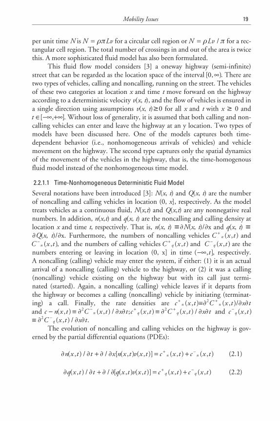
≡ −∂ ∂ ∂2C x t x tq ( , ) / .The evolution of noncalling and calling vehicles on the highway is gov-

erned by the partial differential equations (PDEs):

∂ ∂ ∂ ∂n x t t x n x t v x t c x t c x tn n( , ) / / [ ( , ) ( , )] ( , ) ( , )+ = ++ − (2.1)

∂ ∂ ∂ ∂q x t t q x t v x t c x t c x tq q( , ) / / [ ( , ) ( , )] ( , ) ( , )+ = ++ − (2.2)

Mobility Issues 19

The additional notations are used to show how these, (2.1) and (2.2), arecoupled owing to calling activity. The numbers of noncalling vehicles E x tn

+ ( , )and E x tn

− ( , ), and the numbers of calling vehicles E x tq+ ( , ) and E x tq

− ( , ) areentering or leaving from the highway in location (0, x] in time ( , ]−∞ t , respec-tively. The associated rate densities are: e x t E x t x tn n

+ +≡( , ) ( , ) /∂ ∂ ∂2

and e x t E x t x tn n− −≡( , ) ( , ) / ;∂ ∂ ∂2 e x t E x t x tq q

+ +≡( , ) ( , ) /∂ ∂ ∂2 and e x tq− ( , )

≡ −∂ ∂ ∂2 E x t x tq ( , ) / .Furthermore, β( , ) ( , )x t n x t and γ( , ) ( , )x t q x t are the rates at which noncall-

ing and calling vehicles actually depart from the highway at location x at time t,respectively. Additionally, let λ( , ) ( , )x t n x t be the call-initiation rate of noncall-ing vehicles and µ( , ) ( , )x t q x t be the call-termination rate of calling vehicles atlocation x at time t. In the stochastic model, these are stochastic intensities forindividual vehicles; these are actual deterministic flow rates. The rate densitiesc x t c x t c x tn n q+ − +( , ), ( , ), ( , ) and c x tq

− ( , ) are expressed in terms of these parame-ters. The four rate densities are

c x t e x t x t q x tn n+ += +( , ) ( , ) ( , ) ( , )µ (2.3)

c x t x t n x t x t n x tn− = +( , ) ( , ) ( , ) ( , ) ( , )β λ (2.4)

c x t e x t x t n x tq q+ += +( , ) ( , ) ( , ) ( , )λ (2.5)

c x t r x t q x t x t q x tq− = +( , ) ( , ) ( , ) ( , ) ( , )µ (2.6)

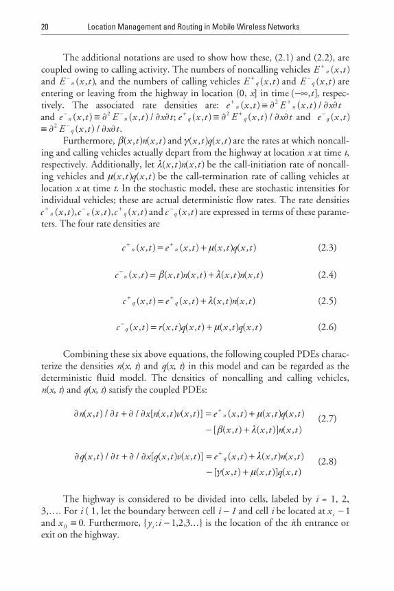
Combining these six above equations, the following coupled PDEs charac-terize the densities n(x, t) and q(x, t) in this model and can be regarded as thedeterministic fluid model. The densities of noncalling and calling vehicles,n(x, t) and q(x, t) satisfy the coupled PDEs:

∂ ∂ ∂ ∂ µn x t t x n x t v x t e x t x t q x tn( , ) / / [ ( , ) ( , )] ( , ) ( , ) ( ,+ = ++ )

[ ( , ) ( , )] ( , )− +β λx t x t n x t(2.7)

∂ ∂ ∂ ∂ λq x t t x q x t v x t e x t x t n x tq( , ) / / [ ( , ) ( , )] ( , ) ( , ) ( ,+ = ++ )

[ ( , ) ( , )] ( , )− +γ µx t x t q x t(2.8)

The highway is considered to be divided into cells, labeled by i = 1, 2,3,…. For i ( 1, let the boundary between cell i – 1 and cell i be located at x i − 1and x 0 0≡ . Furthermore, : , , ...y ii − 1 2 3 is the location of the ith entrance orexit on the highway.


This subsection is concluded by commenting on the rate densities of vehi-cles entering and leaving the highway for the case where vehicles can enter orleave only at entrances and exits at fixed locations, as in real vehicles. Further-more, ξ i

n t( ) and ξ iq t( ) denote the external arrival rate of noncalling and calling

vehicles at the ith entrance at time t, respectively. Then,

e x t t x yn iin i

+ = −( , ) ( ) ( )Σ ξ δ (2.9)

e x t t x yq iiq i

+ = −( , ) ( ) ( )Σ ξ δ (2.10)

where lim ( )εε

ε δ→+

−∫ =0 1xx y dy if x = 0 and 0 otherwise.

As vehicles leave the highway, pin(t) and pi

q(t) denote the fraction of non-calling and calling vehicles departing when they pass by the ith exit at time t,respectively. If these departing vehicles leave at the same velocity as they moveforward along the highway, then

β δ( , ) ( , ) ( ) ( )x t v x t p t x yiin i= −Σ (2.11)

γ δ( , ) ( , ) ( ) ( )x t v x t p t x yiiq i= −Σ (2.12)

2.2.1.2 Time-Homogeneous Deterministic Fluid Model

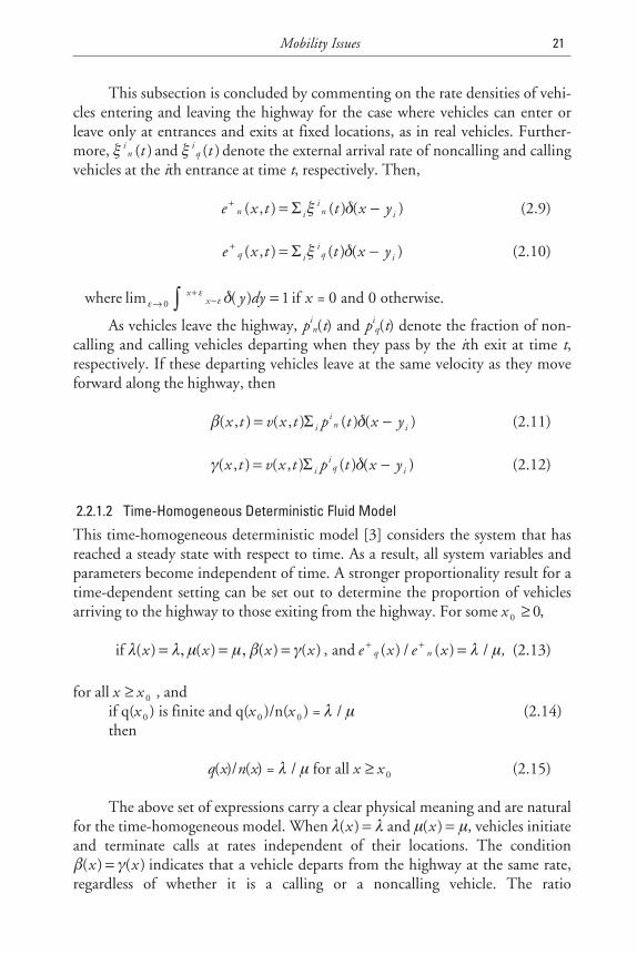
This time-homogeneous deterministic model [3] considers the system that hasreached a steady state with respect to time. As a result, all system variables andparameters become independent of time. A stronger proportionality result for atime-dependent setting can be set out to determine the proportion of vehiclesarriving to the highway to those exiting from the highway. For some x 0 0≥ ,

if λ λ, µ µ, β γ( ) ( ) ( ) ( )x x x x= = = , and e x e xq n+ + =( ) / ( ) /λ µ, (2.13)

for all x x≥ 0 , andif q(x 0 ) is finite and q(x 0 )/n(x 0 ) = λ µ/ (2.14)then

q(x)/n(x) = λ µ/ for all x x≥ 0 (2.15)

The above set of expressions carry a clear physical meaning and are naturalfor the time-homogeneous model. When λ λ( )x = and µ µ( )x = , vehicles initiateand terminate calls at rates independent of their locations. The conditionβ γ( ) ( )x x= indicates that a vehicle departs from the highway at the same rate,regardless of whether it is a calling or a noncalling vehicle. The ratio

Mobility Issues 21

e x e x q x n xq n+ + = =( ) / ( ) ( ) / ( ) /0 0 λ µ means that the proportion of vehicles

arriving to the highway at location x which are calling vehicles is identical to thatof existing vehicles at location x 0 , which, in turn, is equal to the ratio λ µ/ .

One of the limitations of the fluid model is that it describes aggregate traf-fic and therefore is hard to apply to situations where individual movement pat-terns are desired, (e.g., when evaluating network protocols or data managementschemes with caching). Another limitation comes from the fact that since aver-age population density and average velocity are used, this model is more accu-rate for regions containing a large population.

2.2.2 Diffusion Model

A more sophisticated fluid model has been formulated by characterizing theflow of traffic as a diffusion process [4]. A time-varying location probability dis-tribution in conjunction with a Poisson page-arrival model is used to formulatethe paging and registration model in terms of a set of timeout parameters τm .Each timeout parameter is defined as the maximum amount of time to waitbefore registering given in the last known location was m. The simple case ofmemoryless motion is chosen for the clarity of the model. To illustrate thismethod on a time-varying Gaussian user location arises as a result of isotropicrandom user motion. A number of motion models which are specified in termsof independent increments result in Gaussian distributions on location prob-ability. This model would, for example, be used to obtain the minimum averagepaging; each location would be searched in the decreasing order of probability.The mean distribution with equally symmetric locations to either side of themean would give the most likely location.

2.2.3 Gravity Model

Gravity models [1] have been used to model human movement behavior andapplied to regions of varying size, from city models to national and internationalmodels. In its simplest form, the amount of traffic Ti,j moving from region i toregion j is described by: Ti, j = Ki, jPiPj where Pi is the population in region i, andKi, j are parameters that have to be calculated for all possible region pairs (i,j).The different variations of this model usually have to do with the functionalform of Ki, j. For example, analogous to Newton’s gravitational law, Ki, j can bespecified to have inverse square dependence with the distance between zones iand j.

In the above expression, the model describes aggregate traffic and thereforesuffers from some of the same limitations as the fluid model. If Pi is interpretedas the attractivity of region i, however, and Ti,j as the probability of movementsbetween i and j, then the model describes individual movement behavior. Using


TEAMFLY

Team-Fly®

this approach, the parameters Ti, j also have to be calculated from the trafficdata in addition to Ki, j. The advantage of the gravity model is that frequentlyvisited locations can be modeled easily since they are simply regions with largeattractivity. The main difficulty with applying the gravity model is that manyparameters have to be calculated, therefore it is hard to model geography withmany regions.

2.2.4 Random Walk Model

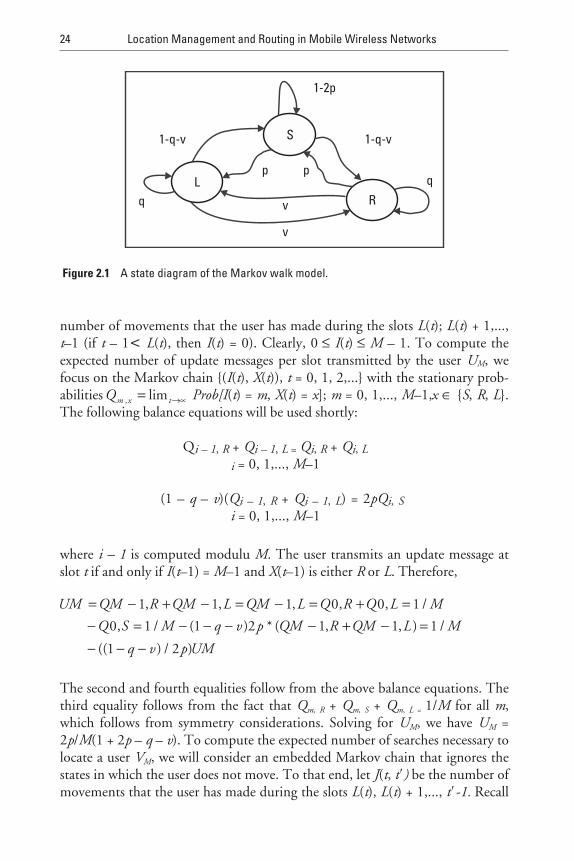
The random walk model [5] is explained with the help of a cellular wirelessradio system with N cells. Two cells are called neighboring cells if a mobile usercan move from one of them to the other without crossing another cell. A ringcellular topology consists of cells where cells i and i + 1 are neighboring cells.Thus, a mobile user that is in cell i, can only move to cells i + 1 or i – 1 orremain in cell i. To model the movement of the mobile users in the system, weassume that time is slotted, and that a user can make at most one move during aslot. The movements will be assumed to be stochastic and independent fromone user to another. Three update strategies are taken: (1) time-based update,(2) movement-based update, and (3) distance-based update to understand theMarkovian random walk model in those strategies. In the Markovian model,during each slot, a user can be in one of the following three states: (1) the sta-tionary state S, (2) the right-move state R, or (3) the left-move state L. Assumethat a user is in cell i at the beginning of a slot. The movement of the user duringthat slot depends on the state as follows. If the user is in state S then it remains incell i, if the user is in state R then it moves to cell i + 1, and if the user is in state Lthen it moves to cell i – 1. Let X(t) be the state during slot t. Assume that X(t); t= 0; 1; 2;... is a Markov chain with transition probabilities pk, l = Prob[X(t + 1) =l = X(t) = k] as follows: pR, R = pL, L = q, pL, R = pR, L = v, pS, R = pS, L = p, pL, S = pR, S = 1– q – v and pS, S = 1 – 2p (see Figure 2.1).

In time-based update, each user transmits an update message every T slots,while in movement-based update, each mobile user transmits an update messagewhenever it completes M movements between cells, and finally in distance-based update, each user transmits an update message whenever the distance, interms of cells, between its current cell and the cell in which it last reported is D.The act of a user sending an update message is referred to as reporting.

For simplicity, only the random walk model for movement-based updateis addressed in this section [5].

Let Y(t) be the distance between the cell in which the user is located in slott and the cell in which the user last transmitted an update message. As before,positive (negative) Y(t) indicates that the user is to the right (left) of the cell fromwhich an update message was last transmitted. Clearly, the interval is –(M–1) ≤Y(t) ≤ M–1. Let L(t) = max |π ≤ t The user reported in slot π . Let I(t) be the

Mobility Issues 23

number of movements that the user has made during the slots L(t); L(t) + 1,...,t–1 (if t – 1< L(t), then I(t) = 0). Clearly, 0 ≤ I(t) ≤ M – 1. To compute theexpected number of update messages per slot transmitted by the user UM, wefocus on the Markov chain (I(t), X(t)), t = 0, 1, 2,... with the stationary prob-abilitiesQm x t, lim= →∝ Prob[I(t) = m, X(t) = x]; m = 0, 1,..., M–1,x ∈ S, R, L.The following balance equations will be used shortly:

Qi – 1, R + Qi – 1, L = Qi, R + Qi, L

i = 0, 1,..., M–1

(1 – q – v)(Qi – 1, R + Qi – 1, L) = 2pQi, Si = 0, 1,..., M–1

where i – 1 is computed modulu M. The user transmits an update message atslot t if and only if I(t–1) = M–1 and X(t–1) is either R or L. Therefore,

UM QM R QM L QM L Q R Q L M

Q S M

= − + − = − = + =− = − −

1 1 1 0 0 1

0 1 1

, , , , , /

, / ( q v p QM R QM L M

q v p UM

− − + − =− − −

) * ( , , ) /

(( ) / )

2 1 1 1

1 2

The second and fourth equalities follow from the above balance equations. Thethird equality follows from the fact that Qm, R + Qm, S + Qm, L = 1/M for all m,which follows from symmetry considerations. Solving for UM, we have UM =2p/M(1 + 2p – q – v). To compute the expected number of searches necessary tolocate a user VM, we will consider an embedded Markov chain that ignores thestates in which the user does not move. To that end, let J(t, t′) be the number ofmovements that the user has made during the slots L(t), L(t) + 1,..., t′-1. Recall


L

S

R

1-q-v 1-q-v

p p

v

v

1-2p

q

q

Figure 2.1 A state diagram of the Markov walk model.

that ts is the slot in which a search occurs. Let tm = max t ≥ L(ts) J(ts, t) = m.The embedded Markov chain is (Y(tm), X(tm)), m = 0, 1, 2,.... Let Pm(d, xx′)= Prob[Y(tm) = d; X(tm) = x X(t0) = x′]. From the definition of tm, it follows thatY(t0) = 0). Define P′m(d, xx′) = Pm(d, xx′) + Pm(–d, xx′) for d >0, and letP′m(dx′) = P′m(d, Rx′) + P′m(d, Lx′). By symmetry considerations, wehave that P′m(dR) = P′m(dL) for all d >0 and m ≥0. The probability that auser will be at an absolute distance d (from the cell from which an update mes-sage was last transmitted) at time tm, namely after m movements, is, therefore,

P′m(d) = P′m(dR) Prob[X(t0) = R] + P′m(dL) Prob[X(t0) = L] = P′m(d(R)

Returning to the Markov chain,

Prob[Y(ts) = d] =Μ = 0

Μ −1

∑ Prob[Y(ts) = dI(ts) = m]* Prob[I(ts) = m]

=Μ = 0

Μ −1

∑ P′m (d )* 1/M

Therefore, the expected number of searches required to locate the user is

SM = 1 + 1/MΜ = 0

Μ −1

∑d =

Μ −1

1∑ DPm(d )

where the latter sum is taken only for even d + m.To complete the computation, we only need to have the quantities Pm(d,

RR ) and Pm(d, LR) for 0 ≤ d, m ≤M–1, and

P0(0, RR ) = (1 + q – v) ⁄ 2

P0(0, LR )= (1 – q + v) ⁄ 2

P0(d, xR ) = 0, d ≠ 0; x ∈R, L

Pm d R R q v Pm d R R

q v Pm d

( , | ) ( ) / * ( , | )

( ) / * (

= + − − −+ − + −

1 2 1 1

1 2 1 +1, | )L R

m ≥ 1, (M–1)≤ d ≤M–1

Mobility Issues 25

Pm d L R q v Pm d R R

q v Pm d

( , | ) ( ) / * ( , | )

( ) / * (

= − + − −+ + − −

1 2 1 1

1 2 1 +1, | )L R

m ≥1, (M–1)≤ d ≤M–1

These probabilities can be computed recursively from the above relations.Using transform techniques, one may obtain expressions for these probabilities.

2.3 Mobility in 3G Systems

2.3.1 Metropolitan Mobility

The three basic types of modeling are appropriate for the discussion of metro-politan mobility. The three types of models city area, area zone, and street unitare introduced [6].

2.3.1.1 City Area Model

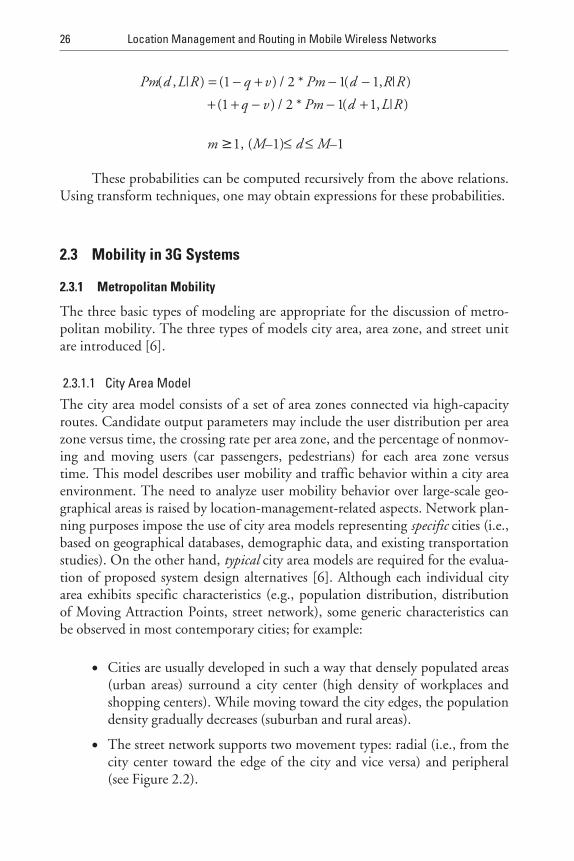
The city area model consists of a set of area zones connected via high-capacityroutes. Candidate output parameters may include the user distribution per areazone versus time, the crossing rate per area zone, and the percentage of nonmov-ing and moving users (car passengers, pedestrians) for each area zone versustime. This model describes user mobility and traffic behavior within a city areaenvironment. The need to analyze user mobility behavior over large-scale geo-graphical areas is raised by location-management-related aspects. Network plan-ning purposes impose the use of city area models representing specific cities (i.e.,based on geographical databases, demographic data, and existing transportationstudies). On the other hand, typical city area models are required for the evalua-tion of proposed system design alternatives [6]. Although each individual cityarea exhibits specific characteristics (e.g., population distribution, distributionof Moving Attraction Points, street network), some generic characteristics canbe observed in most contemporary cities; for example:

• Cities are usually developed in such a way that densely populated areas(urban areas) surround a city center (high density of workplaces andshopping centers). While moving toward the city edges, the populationdensity gradually decreases (suburban and rural areas).

• The street network supports two movement types: radial (i.e., from thecity center toward the edge of the city and vice versa) and peripheral(see Figure 2.2).


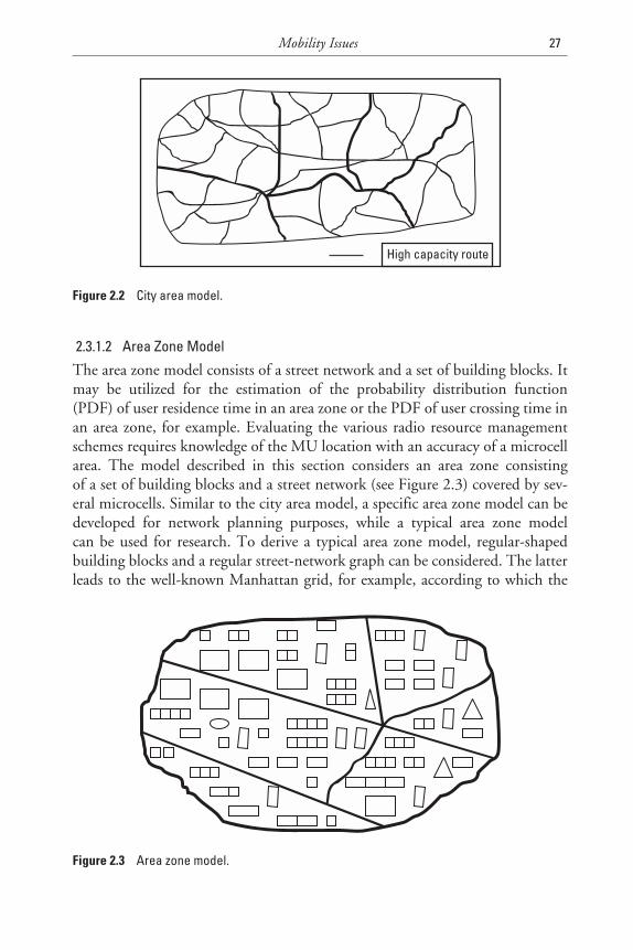
2.3.1.2 Area Zone Model

The area zone model consists of a street network and a set of building blocks. Itmay be utilized for the estimation of the probability distribution function(PDF) of user residence time in an area zone or the PDF of user crossing time inan area zone, for example. Evaluating the various radio resource managementschemes requires knowledge of the MU location with an accuracy of a microcellarea. The model described in this section considers an area zone consistingof a set of building blocks and a street network (see Figure 2.3) covered by sev-eral microcells. Similar to the city area model, a specific area zone model can bedeveloped for network planning purposes, while a typical area zone modelcan be used for research. To derive a typical area zone model, regular-shapedbuilding blocks and a regular street-network graph can be considered. The latterleads to the well-known Manhattan grid, for example, according to which the

Mobility Issues 27

High capacity route

Figure 2.2 City area model.

Figure 2.3 Area zone model.

square-shaped building blocks and an orthogonal grid street network representan area zone [6].

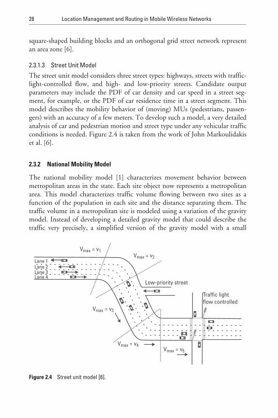
2.3.1.3 Street Unit Model

The street unit model considers three street types: highways, streets with traffic-light-controlled flow, and high- and low-priority streets. Candidate outputparameters may include the PDF of car density and car speed in a street seg-ment, for example, or the PDF of car residence time in a street segment. Thismodel describes the mobility behavior of (moving) MUs (pedestrians, passen-gers) with an accuracy of a few meters. To develop such a model, a very detailedanalysis of car and pedestrian motion and street type under any vehicular trafficconditions is needed. Figure 2.4 is taken from the work of John Markoulidakiset al. [6].

2.3.2 National Mobility Model

The national mobility model [1] characterizes movement behavior betweenmetropolitan areas in the state. Each site object now represents a metropolitanarea. This model characterizes traffic volume flowing between two sites as afunction of the population in each site and the distance separating them. Thetraffic volume in a metropolitan site is modeled using a variation of the gravitymodel. Instead of developing a detailed gravity model that could describe thetraffic very precisely, a simplified version of the gravity model with a small


V = vmax 1V = vmax 2

V = vmax 3

V = vmax 5V = vmax 4

Low-priority streetLane 4Lane 3Lane 2Lane 1

Traffic lightflow controlled

Figure 2.4 Street unit model [6].

number of parameters is used to model [1] this movement. Assuming symmetrictraffic flow, (i.e., the traffic volumes between any two metropolitan areas are thesame along both directions), the national mobility model is a realistic and rea-sonable model for movements between metropolitan areas. In addition, thismodel [1] is relatively insensitive to parameter variations and is reasonable to usein estimating traffic volumes in the future or for other geographies.

2.3.3 International Mobility Model

The international mobility model [1] characterizes movement behavior betweenone country and other countries. Each site object in this model represents acountry. Compared to the national mobility model, the international gravitymodel is missing the inverse dependence on distance. One reason is thatthere is uncertainty in defining distances between countries. Defining the dis-tance between the United States and Canada, two large territories, is a goodexample. In any case, the goal is to have a simple, easy-to-use, realistic model forinternational movement traffic.

References

[1] Lam, Derek., Donald C. Cox, and Jennifer Widom., “Teletraffic Modeling for PersonalCommunications Services,” IEEE Communications Magazine, Feb. 1997, pp. 79–87.

[2] Frost, V. S., and B. Melamed, “Traffic Modeling for Telecommunications Networks,”IEEE Communications Magazine, March 1994, pp. 70–81.

[3] Leung, K. K., W. A. Massey, and W. Whitt, “Traffic Models for Wireless Communica-tion Networks,” IEEE JSAC, Oct. 1994, pp. 1353–1364.

[4] Rose, C., “Minimizing the Average Cost of Paging and Registration: A Timer-BasedMethod,” ACM J. Wireless Networks, Feb. 1996, pp. 109–116.

[5] Bar-Noy, A., and I. Kessler, “Mobile Users: To Update or Not To Update?” Proc.INFOCOM 94, June 1994, pp. 570–576.

[6] Markoulidakis, John G., et al., “Mobility Modeling in Third-Generation Mobile Tele-communications Systems,” IEEE Personal Communications, Aug. 1997, pp. 41–56.

Mobility Issues 29

.

3Radio Resource Management

The rapid increase in the size of the wireless mobile community and theirdemands for high-speed, multimedia communications stands in clear contrast tothe limited spectrum resource that has been allocated to them in internationalagreements. Comparing market estimates for wireless mobile communicationand considering recent proposals for wideband multimedia services with theexisting spectrum allocations shows that spectrum resource managementremains an important topic for the foreseeable future. Efficient spectrumresource management is, therefore, of paramount importance. In this chapter,we begin with a brief introduction to what is meant by radio resource, then pres-ent an overview of the solutions to the radio resource management (RRM)problem and finally, outline the key problems of resource management in next-generation wireless networks.

The network under consideration has already been introduced in Chap-ter 1. For the sake of continuity, we reiterate it briefly here. It consists of a fixednetwork part and a wireless access system. The fixed network provides connec-tions between BSs, which in turn provide the wireless connections to the mobileterminals (MTs). BSs are normally distributed over the complete geographicalarea (service area) where the mobile users are provided with communicationservices. In two-way communication systems (such as mobile telephone sys-tems), links have to be established both from the BS to the mobile (downlink orforward link) and from the mobile terminal to the BS (uplink or reverse link).The propagation situation is quite different, particularly in wide-area cellularphone systems, where the BS usually has its antennas at some elevated location,free of obstacles. The terminals, on the other hand, are usually located amidstbuildings and other obstacles, creating shadowing and multipath reflections.

31

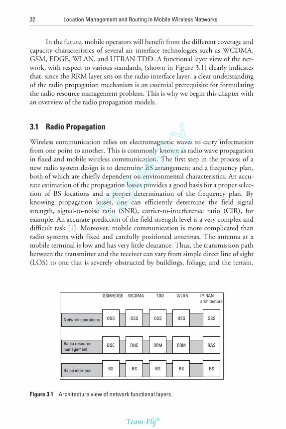
In the future, mobile operators will benefit from the different coverage andcapacity characteristics of several air interface technologies such as WCDMA,GSM, EDGE, WLAN, and UTRAN TDD. A functional layer view of the net-work, with respect to various standards, (shown in Figure 3.1) clearly indicatesthat, since the RRM layer sits on the radio interface layer, a clear understandingof the radio propagation mechanism is an essential prerequisite for formulatingthe radio resource management problem. This is why we begin this chapter withan overview of the radio propagation models.

3.1 Radio Propagation

Wireless communication relies on electromagnetic waves to carry informationfrom one point to another. This is commonly known as radio wave propagationin fixed and mobile wireless communication. The first step in the process of anew radio system design is to determine BS arrangement and a frequency plan,both of which are chiefly dependent on environmental characteristics. An accu-rate estimation of the propagation losses provides a good basis for a proper selec-tion of BS locations and a proper determination of the frequency plan. Byknowing propagation losses, one can efficiently determine the field signalstrength, signal-to-noise ratio (SNR), carrier-to-interference ratio (CIR), forexample. An accurate prediction of the field strength level is a very complex anddifficult task [1]. Moreover, mobile communication is more complicated thanradio systems with fixed and carefully positioned antennas. The antenna at amobile terminal is low and has very little clearance. Thus, the transmission pathbetween the transmitter and the receiver can vary from simple direct line of sight(LOS) to one that is severely obstructed by buildings, foliage, and the terrain.


Network operations

GSM/EDGE WCDMA TDD WLAN IP-RANarchitecture

OSS OSS OSS OSS OSS

Radio resourcemanagement

BSC RNC RRM RRM RAS

Radio interface BS BS BS BS BS

Figure 3.1 Architecture view of network functional layers.

TEAMFLY

Team-Fly®

Coverage problems due to various propagation effects put a lower limit on thenumber of BSs required.

The mobile radio channel is evaluated from statistical propagation models:specific terrain data is considered, and channel parameters are modeled as sto-chastic variables. The mean signal strength for an arbitrary transmitter-receiver(T-R) separation is useful in estimating the radio coverage of a given transmitter,whereas measures of signal variability are key determinants in system designissues, such as antenna diversity and signal coding. The modeling of the propa-gation path needs to take into account a number of effects. These include thefollowing:

1. Path loss: The signal gets reduced in power with the distance it traver-ses following an inverse square law.

2. Shadowing: Scattering environments along various propagation pathswill be different, causing variations with respect to the nominal valuegiven by the path loss. Some paths will suffer increased loss, while oth-ers will be less obstructed and have an increased signal strength. Thisphenomenon is called shadowing or slow fading and is said to followlog-normal fading statistics [1].

3. Number of multipath components and distribution of their envelopes:These effects are caused by the local scattering environment aroundthe MT or BS or both.

4. Temporal fading: The cause of this type of fading can be attributed tolarge-scale fading or small-scale fading. Large-scale fading or shadow-ing has path loss effects (explained in Section 3.1.2). Small-scale fadingmanifests itself in two mechanisms, namely, signal dispersion and timevariant behavior of the channel.

5. Correlation: Multipath components generated by a single area of localscatterers may show considerable correlation, with the correlationdepending heavily on the assumptions made concerning the spatialdistribution of local scattering elements.

3.1.1 Path Loss

If a wireless channel’s propagating characteristics are not specified, it is generallyinferred that the signal attenuation versus distance behaves as if the propagationtakes place over a terrain. The model of free space treats the region between thetransmitting and the receiving antennas as being free of all objects that mightabsorb or reflect RF energy. It is further assumed that, within this region, theatmosphere behaves as a perfectly uniform and nonabsorbing medium. Further-more, the earth is treated as being infinitely far away from the propagating

Radio Resource Management 33

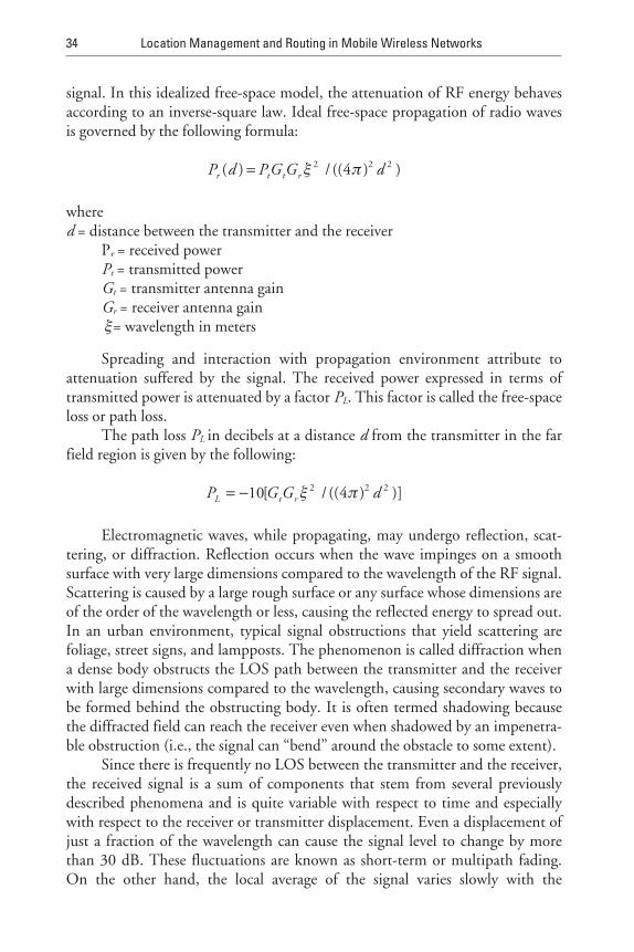
signal. In this idealized free-space model, the attenuation of RF energy behavesaccording to an inverse-square law. Ideal free-space propagation of radio wavesis governed by the following formula:

P d P G G dr t t r( ) / (( ) )= ξ π2 2 24

whered = distance between the transmitter and the receiver

Pr = received powerPt = transmitted powerGt = transmitter antenna gainGr = receiver antenna gainξ= wavelength in meters

Spreading and interaction with propagation environment attribute toattenuation suffered by the signal. The received power expressed in terms oftransmitted power is attenuated by a factor PL. This factor is called the free-spaceloss or path loss.

The path loss PL in decibels at a distance d from the transmitter in the farfield region is given by the following:

P G G dL t r= −10 42 2 2[ / (( ) )]ξ π

Electromagnetic waves, while propagating, may undergo reflection, scat-tering, or diffraction. Reflection occurs when the wave impinges on a smoothsurface with very large dimensions compared to the wavelength of the RF signal.Scattering is caused by a large rough surface or any surface whose dimensions areof the order of the wavelength or less, causing the reflected energy to spread out.In an urban environment, typical signal obstructions that yield scattering arefoliage, street signs, and lampposts. The phenomenon is called diffraction whena dense body obstructs the LOS path between the transmitter and the receiverwith large dimensions compared to the wavelength, causing secondary waves tobe formed behind the obstructing body. It is often termed shadowing becausethe diffracted field can reach the receiver even when shadowed by an impenetra-ble obstruction (i.e., the signal can “bend” around the obstacle to some extent).

Since there is frequently no LOS between the transmitter and the receiver,the received signal is a sum of components that stem from several previouslydescribed phenomena and is quite variable with respect to time and especiallywith respect to the receiver or transmitter displacement. Even a displacement ofjust a fraction of the wavelength can cause the signal level to change by morethan 30 dB. These fluctuations are known as short-term or multipath fading.On the other hand, the local average of the signal varies slowly with the


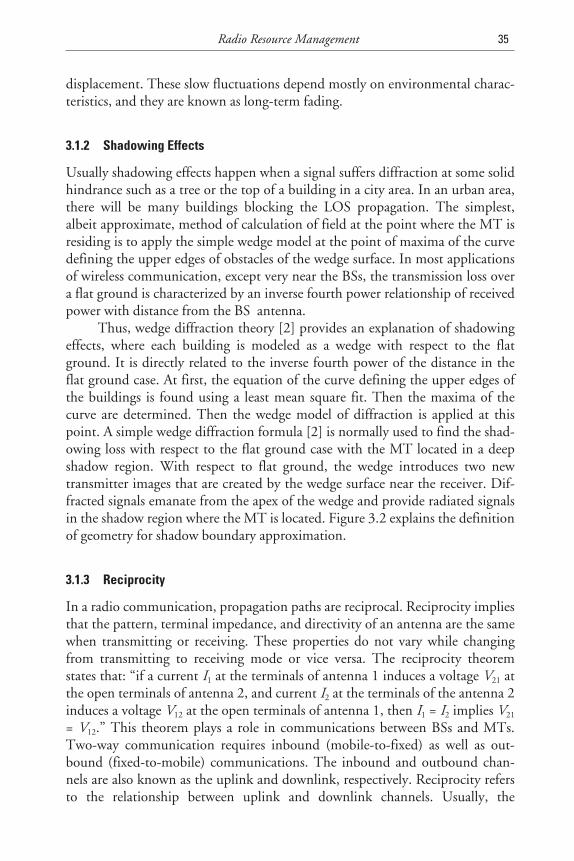
displacement. These slow fluctuations depend mostly on environmental charac-teristics, and they are known as long-term fading.

3.1.2 Shadowing Effects

Usually shadowing effects happen when a signal suffers diffraction at some solidhindrance such as a tree or the top of a building in a city area. In an urban area,there will be many buildings blocking the LOS propagation. The simplest,albeit approximate, method of calculation of field at the point where the MT isresiding is to apply the simple wedge model at the point of maxima of the curvedefining the upper edges of obstacles of the wedge surface. In most applicationsof wireless communication, except very near the BSs, the transmission loss overa flat ground is characterized by an inverse fourth power relationship of receivedpower with distance from the BS antenna.

Thus, wedge diffraction theory [2] provides an explanation of shadowingeffects, where each building is modeled as a wedge with respect to the flatground. It is directly related to the inverse fourth power of the distance in theflat ground case. At first, the equation of the curve defining the upper edges ofthe buildings is found using a least mean square fit. Then the maxima of thecurve are determined. Then the wedge model of diffraction is applied at thispoint. A simple wedge diffraction formula [2] is normally used to find the shad-owing loss with respect to the flat ground case with the MT located in a deepshadow region. With respect to flat ground, the wedge introduces two newtransmitter images that are created by the wedge surface near the receiver. Dif-fracted signals emanate from the apex of the wedge and provide radiated signalsin the shadow region where the MT is located. Figure 3.2 explains the definitionof geometry for shadow boundary approximation.

3.1.3 Reciprocity

In a radio communication, propagation paths are reciprocal. Reciprocity impliesthat the pattern, terminal impedance, and directivity of an antenna are the samewhen transmitting or receiving. These properties do not vary while changingfrom transmitting to receiving mode or vice versa. The reciprocity theoremstates that: “if a current I1 at the terminals of antenna 1 induces a voltage V21 atthe open terminals of antenna 2, and current I2 at the terminals of the antenna 2induces a voltage V12 at the open terminals of antenna 1, then I1 = I2 implies V21

= V12.” This theorem plays a role in communications between BSs and MTs.Two-way communication requires inbound (mobile-to-fixed) as well as out-bound (fixed-to-mobile) communications. The inbound and outbound chan-nels are also known as the uplink and downlink, respectively. Reciprocity refersto the relationship between uplink and downlink channels. Usually, the


interference situation in the uplinks and downlinks will be different since thereare many terminals, varying locations and quite a few BSs at fixed locations.That is why cellular uplink and downlink paths are normally on different fre-quencies. The consequence of the mobile antenna being low is that the mobile ismore likely to suffer interference.

Multipath scatters mostly occur in the immediate vicinity of the mobileantenna. The BS receives, more or less, a transversal electromagnetic wave,whereas the MS receives a superposition of a set of reflected waves from randomangles. Two antennas at the mobile terminal are likely to receive uncorrelatedsignal powers if their separation is more than a wavelength. At the BS site, how-ever, all reflections arrive from almost identical directions. Therefore, diversityat the BS requires much larger separation of the antennas to ensure uncorrelatedreceived signal powers at the two antennas. For the same reason, antenna direc-tivity has different effects at the mobile terminal (MT) and the BS.

In a cellular network, shadow fading of the wanted signal received by theMS is likely to be correlated with the shadow fading of the interference causedby other BSs, or in a spread-spectrum network, with the shadowing of simulta-neously transmitted signals from the same BS. In contrast to this, at the BS,shadow fading of the wanted signal is mostly statistically independent fromshadow fading of the interference. However, experimental results for correlationof shadow attenuation are scarce. In full-duplex operation, multipath fading of


Tx

α

D1

Y1Y2

Ym

D2

MT

X1 X2 Xm(X ,Y ): Coordinate of building 1(X ,Y ): Coordinate of building mT : Transmitting antennaD : Distance from T to knife edge at (X , Y )D : Distance from T to knife edge at (X , Y ) to the MT

: the angle subtended by the straight line joining the T andthe top knife edge at (X ,Y ) with a horizontal line

1 1

m m

x

1 X m m

2 X m m

x

m m

α

Figure 3.2 Geometry for shadow boundary approximation.

inbound and outbound channels, which operate at widely different frequencies,may be uncorrelated. This will particularly be the case if the delay spread is large.

In a practical multiuser system with intermittent transmissions, inboundmessages are sent via a multiple-access channel, whereas in an outbound chan-nel, signals destined for different users can be multiplexed. In the latter case, thereceiver in a MS can maintain carrier and bit synchronization to the continuousincoming bit stream from the BS, whereas the receiver in the BS has to acquiresynchronization for each user slot. Moreover, in packet-switched data networks,the inbound channel has to accept randomly occurring transmissions by the ter-minals in the service area. In cellular networks with large traffic loads per BS,spread-spectrum modulation can be exploited in the downlink to combat multi-path fading, whereas in the uplink, the signal powers from the various mobilesubscribers may differ too much to effectively apply spread-spectrum multipleaccess unless sophisticated adaptive power control techniques are employed.

3.1.4 Indoor Wireless

There are several causes of signal corruption in an indoor wireless channel. Theprimary causes are signal attenuation due to distance, penetration losses throughwalls and floors, and multipath propagation. Signal attenuation over distance isobserved when the mean received signal power is attenuated as a function of thedistance from the transmitter (the free-space loss described above). Multipathresults from the fact that the propagation channel consists of several obstaclesand reflectors. Thus, the received signal arrives as an unpredictable set of reflec-tions or direct waves or both, each with its own degree of attenuation and delay.The delay spread is a parameter commonly used to quantify multipath effects.Multipath leads to variations in the received signal strength over frequency andantenna location. For wireless LANs this could mean that an antenna placed in alocal multipath null, remains in fade for a very long time. Measures such asdiversity are needed to guarantee reliable communication irrespective of theposition of the antenna. Wideband transmission, (e.g., direct sequenceCDMA), could provide frequency diversity.

3.2 Radio Resource (Spectrum Allocation)

Clearly the radio resource (i.e., air interface) will continue to be the most limitedresource in mobile operators’ networks. Managing these multiple resourcestogether, as a single resource pool, will be the key to maximizing the utilizationof the operator’s resources.


3.2.1 Radio Frequency Spectrum Allocation

In the United States, the Federal Communications Commission (FCC) and theNational Telecommunications and Information Administration (NTIA) man-age the radio frequency spectrum through a system of frequency allocations,allotments, and assignments. The entire radio spectrum is divided into blocks,or bands, of frequencies established for a particular type of service by the processof frequency allocation. Further, these general allocations can be subdivided intobands designated for a particular service, or allotment. Within these subdividedbands, specific channel plans may be implemented. For example, allocationsmade to the land mobile service are divided into allotments for business users,public safety users, and cellular users, with each group allotted a portion of theband in which to operate. Assignment refers to the final subdivision of the spec-trum in which a party gets an assignment, or license, to operate a radio transmit-ter on a specific channel or group of channels at a particular location underspecific conditions. The FCC also issues some licenses on a more general geo-graphic basis. The FCC has listed U.S. allocations in a table of frequency alloca-tions that can be found in Section 2.106 of the Commission’s rules (http://www.fcc.gov/oet/info/rules).

3.2.2 International Allocations

International coordination of spectrum is a critical component of the spectrumallocation process because radio waves transcend national borders and becauseof the increasing number of global services. The radio communication con-ferences of the International Telecommunication Union (ITU) are the prin-cipal mechanisms for international spectrum allocation. The ITU’s table of al-locations represents a global consensus that reflects the needs of ITU mem-berstates. The scheduling of conferences every two to three years with a specifiedagenda keeps the table of allocations flexible and current. Its general success isevidenced by, for example, the allocations provided during the 1992 conferencefor mobile-satellite services that are now coming into use. These conferencesmay address any service throughout the entire radio spectrum, depending on theagendas set by the ITU Council. In addition, there are also Regional RadioCommunication Conferences, which meet as necessary and have a restrictedagenda devoted to specific services for the ITU region concerned. Based on theagreements reached at these conferences, the ITU publishes the internationalRadio Regulations, which include allocations and technical rules for radiooperation for each of the three regions of the world (http://www.fcc.gov/ib/WRC00). The ITU further designates such allocations as primary orsecondary.


• Primary allocations grant priority to specific services in using theallocated spectrum. When there are multiple primary services withina frequency band, they all have equal rights. A station, however, hasthe right to be protected from any others that start operation at a laterdate.

• Secondary allocations are made for services that must protect all primaryallocations in the same band. Services operating in secondary alloca-tions must not cause harmful interference to, and must accept interfer-ence from, primary service stations. All secondary service stations haveequal rights among themselves in the same frequency band.

3.2.3 Financing for Spectrum Management

Every country faces challenges in ensuring that its spectrum regulatory body hassufficient funding to meet the costs of spectrum management. License fees rep-resent one way to improve the economic and technical efficiency of nationalspectrum management. At the FCC, two types of fees are collected, applicationfees and regulatory fees, to cover the cost of allocating the use the spectrum. Inaddition to paying for the administrative cost of managing the use of the spec-trum, the fees may also serve to discourage the filing of frivolous applications. Ifset too high, however, fees can result in underutilization of the spectrum(http://www.fcc.gov/fees).

3.2.4 Spectrum Monitoring and Enforcement

Effective spectrum monitoring and enforcement requires tools to ensure adher-ence to spectrum allocation and use regulations, as well as identification andelimination of interference. The United States uses a variety of tools to monitorspectrum use and enforce adherence to U.S. rules and regulations. Among thesetools are (1) databases of information on licensed systems; (2) information, inthe form of national rules on general licensing and technical requirements con-cerning specific services; (3) electronic equipment for determining the sources ofinterference and illegal radio operations; and (4) regulatory mechanisms forassessing penalties on licensees not complying with regulations.

In both the domestic and international context, maintaining a database ofrelevant technical parameters on individual communications systems is one toolnecessary for monitoring compliance with spectrum use regulations. In cases ofcomplaints of noncompliance with regulations, the regulator need merely accessthe database to obtain technical parameters to help determine whether a stationis in compliance.


In some cases, it is not practical to maintain a database on all licensedsystems and their components. For example, many systems communicate withconsumer handsets that are not individually licensed. In these cases, codifyinggeneral licensing conditions and technical requirements in a rulebook providesa basis for determining compliance. With either a database of actual systemparameters or a rulebook stating required conditions, spectrum regulators canconduct engineering and managerial analyses to ensure that operators complywith the relevant technical rules for spectrum use.

Identifying interference sources is also a critical component of ensuringcompliance with spectrum use rules. At the FCC, the electronic direction finderhas proven to be highly effective for pinpointing interference sources and tak-ing measures to eliminate interference. If an interference complaint is received,the direction finder can be used to locate an interfering transmitter. In domes-tic cases of interference, a letter can be sent to the operator of the interferingstation or a physical investigation of the transmitting site can be made. In thecase of interference from international sources, a special note is sent to theadministration of the offending operator, informing that administration of theinfringement.

In cases of repeated interference or illegal operations, the FCC has theauthority to assess penalties on the offending party. For this type of action tobe effective, penalties related to specific violations must be clearly defined andpublicized. Depending on the severity of the infraction, penalties can includewarnings, fines, revocation of license, equipment seizure, and, in severe cases,incarceration.

There is an enormous pent-up demand for access to radio waves, andhigh barriers to entry imposed by regulators are stifling substantial economicgrowth. But this is because the spectrum allocation is working precisely asplanned. Regulation serves to protect incumbent interests for a modest sur-charge, a public interest tax that the tax collector more often than not forgetsto collect.

The FCC’s continuing (mis)management of the TV Band is noteworthywhen the TV Band is being reduced to irrelevance. A linear extrapolation ofthe prices paid for PCS licenses in a January 2001 FCC auction imply that thespectrum allocated to the TV Band would fetch up to $470 billion—if theycould be used for something other than TV. More importantly, consumer bene-fits are likely to easily exceed this number. For instance, the GSM association isattempting to gain widespread acceptance of the spectrum strategy by thefollowing:

• Requesting administrators and lobbying regional telecommunicationorganizations to release the designated by the ITU in 1992;


• Inviting administrators and regional telecommunication organizationsto support and propose the Association’s views on and associated regu-latory at World Radiocommunication Conference (WRC-2000).

Concerning the first item above, regulatory authorities are encouraged torelease sufficient IMT-2000 core-band spectrum to facilitate the introduction of3GSM IMT-2000 services utilizing the GSM platform from 2002. A good start-ing point would be 2 × 15 MHz + 5 MHz (i.e., 35 MHz) per operator in the ini-tial phase, moving towards the release of the entire 155 to 175 MHz within thecore band before 2005. This is the spectrum designated for IMT-2000 atWARC-92 (World Administrative Radio Conference, 1992).

Of equal importance is the global release of the existing second-generationbands for second-generation GSM services. This would for example mean thatspectrum between 862 and 960 MHz and the totality of the GSM1800 band,1,710 to 1,880 MHz, should be released before 2002 for mobile applications aswidely as possible.

3.2.5 GSM Frequencies

In principle, the GSM system can be implemented in any frequency band.However there are several bands where GSM terminals are, or will shortly be,available. Furthermore, GSM terminals may incorporate one or more of theGSM frequency bands listed below to facilitate roaming on a global basis.

• GSM400: 450.4 to 457.6 MHz paired with 460.4 to 467.6 MHz or478.8 to 486 MHz paired with 488.8 to 496 MHz;

• GSM 850: 824 to 849 MHz (mobile transmit, base receive), 869 to894 MHz (base transmit, mobile receive);

• GSM900: 880 to 915 MHz paired with 925 to 960 MHz;

• GSM1800: 1,710 to 1,785 MHz paired with 1,805 to 1,880 MHz;

• GSM1900: 1,850 to 1,910 MHz paired with 1,930 to 1,990 MHz.

In the above bands, MSs transmit in the lower frequency subband and BSstransmit in the higher frequency subband.

3.2.6 IMT-2000 (Third-Generation) Core Frequency Band

The third-generation frequencies for IMT-2000 were identified by the ITU in1992 and appear as No. S5.388 of the Radio Regulations:


S5.388 The bands 1,885 to 2,025 MHz and 2,110 to 2,200 MHz areintended for use on a worldwide basis by administrations wishing to implementIMT-2000. Such use does not preclude the use of these bands by other servicesto which they are allocated. The bands should be made available for IMT-2000in accordance with Resolution 212 (Rev.WRC-97).

Terrestrial IMT-2000 services will operate in the Frequency DivisionDuplex (FDD) mode in the bands 1,920 to 1,980 MHz paired with 2,110 to2,170 MHz with MSs transmitting in the lower subband and BSs transmittingin the upper subband. The bands 1,885 to 1,920 MHz and 2,010 to 2,025MHz are unpaired for Time Division Duplex (TDD) operation. Administra-tions and Regional Regulatory Telecommunication Organizations should beconsulted concerning any specific national or regional arrangements forIMT-2000.

GSM association members will, subject to commercial, operational, andregulatory considerations, commence the introduction of third-generationIMT-2000 services from 2002.

3.2.7 IMT-2000 (Third-Generation) Extension Bands

At the May to June 2000 World Radiocommunication Conference(WRC-2000) the ITU identified additional IMT-2000 frequency bands.

In addition to the frequency bands currently designated for IMT-2000 innumber S5.388 of the Radio Regulations (the IMT-2000 core-band) and thosebands which in 2005 will be utilized by administrations for second-generationpublic land mobile services in their territories (e.g., GSM 900, 1,800, and1,900), the frequency bands 698 to 806 MHz, 2,500 to 2,690 MHz, and 2,700to 2,900 MHz should be nonexclusively designated for the use of IMT-2000 toprovide for up to an additional 160 MHz of spectrum for IMT-2000 from2005. Subject to commercial demand, the 160 MHz of additional spectrumshould be available in its entirety prior to 2010. Existing second-generationbands (including GSM bands) 806 to 960 MHz, 1,429 to 1,501 MHz and1,710 to 1,885 MHz should be confirmed as very long term IMT-2000 bandsand studies commenced to pave their way for formal identification at a subse-quent WRC. These were not be identified at WRC-2000 as IMT-2000 exten-sion bands since they will continue to be extensively used for GSM (and othersecond-generation systems) for a long period of time for both GSM and in mul-timode GSM IMT-2000 terminals to supplement IMT-2000 coverage. All thebands (extension and existing second-generation bands) should be allocated inall ITU regions on a primary basis to the mobile service (if not already so allo-cated) in the ITU Radio Regulations.

Today’s market estimates for mobile wireless personal communication andconsidering 3G and 4G proposals for wideband multimedia services show that


TEAMFLY

Team-Fly®

spectrum resource management will remain an important aspect in the nearfuture. As the number of transmitters in the system becomes large within somefixed chunk of available RF spectrum, the number of simultaneous connections(links) will become larger than the number of orthogonal signals the availablebandwidth may provide.

3.3 RRM

By now, it should be clear to the readers that, in order to better utilize the scarceradio spectrum in mobile communication systems, the available radio resources(transmitter powers, channels, and BSs) must be used in the most efficient way.Efficient use of radio spectrum [3] is important from a cost-of-service point ofview, where the number of BSs required to service a given geographical area is animportant factor. A reduction in the number of BSs, and hence in the cost ofservice, can be achieved by more efficient reuse of the radio spectrum. All RRMschemes are designed using some model for the traffic. Most wireless systemstoday use circuit-switched speech as the main design model (e.g., GSM, CDMAone). Future wireless access systems are expected to carry both voice and data aswell as a mixture of services with very different and often conflicting servicerequirements.

3.3.1 RRM Problem

We describe the RRM problem as formulated in [4]. Let us assume that Mmobiles are served by BSs, numbered from the set B = 1, 2, 3,..., B. Let us alsoassume that there are C orthogonal channel pairs numbered from the set C = 1,2, 3,..., C available for establishing links between BSs and MTs. To establishradio links, the system has to assign to each mobile: (1) a BS from the set B, (2) achannel from the set C, and (3) a transmitter power for the access port and theterminal. This assignment is performed according to the resource allocationalgorithm (RAA) of the wireless communication system. The assignment isrestricted by the interference caused by the BSs and mobiles as soon as they areassigned a channel and when they start using it. Another common restriction isthat BSs, in many cases, use only a subset of the available channels. Good alloca-tion schemes will aim at assigning links with adequate signal-to-interferenceratio (SIR) to as many (possibly all) mobiles as possible. Note that the RAA maywell (should) opt for not assigning a channel to an active mobile if this assign-ment would cause excessive interference to other mobiles.

Let us now study the interference constraints on resource allocations insomewhat more detail. We now may compute the signal and interference powerlevels in all access ports and mobiles, given the link (power) gains, Gij, between


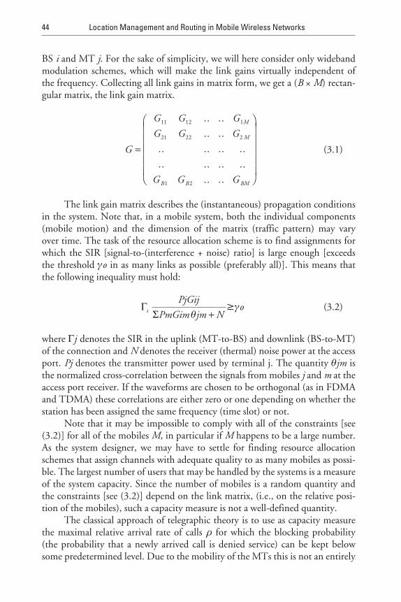
BS i and MT j. For the sake of simplicity, we will here consider only widebandmodulation schemes, which will make the link gains virtually independent ofthe frequency. Collecting all link gains in matrix form, we get a (B × M) rectan-gular matrix, the link gain matrix.

G

G G G

G G G

G G

M

M

B B

=

11 12 1

21 22 2

1 2

.. ..

.. ..

.. .. .. ..

.. .. .. ..

.. .. G BM

(3.1)

The link gain matrix describes the (instantaneous) propagation conditionsin the system. Note that, in a mobile system, both the individual components(mobile motion) and the dimension of the matrix (traffic pattern) may varyover time. The task of the resource allocation scheme is to find assignments forwhich the SIR [signal-to-(interference + noise) ratio] is large enough [exceedsthe threshold γo in as many links as possible (preferably all)]. This means thatthe following inequality must hold:

ΓΣι θ

PjGij

PmGim jm N+≥γo (3.2)

where Γj denotes the SIR in the uplink (MT-to-BS) and downlink (BS-to-MT)of the connection and N denotes the receiver (thermal) noise power at the accessport. Pj denotes the transmitter power used by terminal j. The quantity θjm isthe normalized cross-correlation between the signals from mobiles j and m at theaccess port receiver. If the waveforms are chosen to be orthogonal (as in FDMAand TDMA) these correlations are either zero or one depending on whether thestation has been assigned the same frequency (time slot) or not.

Note that it may be impossible to comply with all of the constraints [see(3.2)] for all of the mobiles M, in particular if M happens to be a large number.As the system designer, we may have to settle for finding resource allocationschemes that assign channels with adequate quality to as many mobiles as possi-ble. The largest number of users that may be handled by the systems is a measureof the system capacity. Since the number of mobiles is a random quantity andthe constraints [see (3.2)] depend on the link matrix, (i.e., on the relative posi-tion of the mobiles), such a capacity measure is not a well-defined quantity.

The classical approach of telegraphic theory is to use as capacity measurethe maximal relative arrival rate of calls ρ for which the blocking probability(the probability that a newly arrived call is denied service) can be kept belowsome predetermined level. Due to the mobility of the MTs this is not an entirely


satisfying measure. A call may be lost due to adverse propagation conditions. Toinclude such phenomena into the above formulation, we would require detailedspecification of call handling procedures (e.g., handling of new versus old calls,handoff procedures as a mobile moves from one access port to another). It maytherefore be practical to choose a simpler and more fundamental capacity meas-ure that will reflect the performance of the resource allocation scheme as such.

For this purpose, let us assume that, at some given instant, the RAA hassucceeded in providing adequate links to a number of MTs Y out of the totalnumber M. Y will of course be a stochastic variable. Let Z denote the remainingnumber of mobiles, for which the assignment fails, that is

Z = M – Y (3.3)

We define the assignment failure rate ν as

ν =E ZE M

[ ]

[ ]=

E MA

[ ]

ω(3.4)

In the last expression we have assumed the (active) MTs to be uniformly(2D Poisson) distributed over the service area A with ω mobiles per area unit.The quantity ν is a measure of the extent to which the allocation scheme hasbeen successful in providing the MTs with links of adequate quality. For moder-ate to large ωA, ν is also a good approximation of the probability that a ran-domly chosen active mobile at some given instant is not provided with achannel. The instantaneous capacity ω* ( )νo of a wireless system is the maxi-mum allowed traffic load in order to keep the assignment failure rate belowsome threshold level ν 0 , that is,

ω*( )νo = max ω : ν ≤ νo (3.5)

As we have seen above, it is a formidable problem to find the optimumresource allocation, that is, to determine for each MT the following:

1) A waveform assignment (determining the θjm);

2) A BS assignment [of one or more (!) ports];

3) A transmitter power assignment that maximizes Y for a given link gainmatrix.

No efficient general algorithm that is capable of doing such an optimalassignment for arbitrary link gain matrices and mobile sets is known [3].Instead, partial solutions and a number of more or less complex heuristicschemes have been proposed (and are used in the wireless systems of today).These schemes are usually characterized by low complexity and by using simple


heuristic design rules. The capacity ω* achieved by these schemes is, asexpected, often considerably lower than what could be expected by optimumchannel assignment.

3.3.2 Channel Allocation and Assignment

An interesting subproblem of the general RRM problem that has attractedmuch attention in the literature is the choice and allocation of channels. Divid-ing the spectrum into a set of channels (i.e., identifying C ) is the first step inRRM. A given radio spectrum (or bandwidth) can be divided into a set of dis-joint or noninterfering radio channels. All such channels can be used to main-tain an acceptable received radio signal. Many techniques, such as frequencydivision (FD), time division (TD), or code division (CD), can be used in orderto divide a given radio spectrum into channels (i.e., a “channelization” of thespectrum). In FD, the spectrum is divided into disjoint frequency bands, whilein TD the channel separation is achieved by dividing the usage of the channelinto disjoint time periods called time slots. In CD, the channel separation isachieved by using different modulation codes. Also, dividing each frequencyband of an FD scheme into time slots can use a combination of TD and FD.The major driving factor in determining the number of channels with certainquality that can be used for a given wireless spectrum is the level of received sig-nal quality that can be achieved in each channel. Classical orthogonalizationtechniques, such as FDMA and TDMA are very common and used extensivelyin various systems. They are now being challenged, however, by nonorthogonalwaveform systems of CDMA such as IS-95 [5–8].

Once the set C is known, the next problem is the assignment of waveformsto the different terminal access port links. This is known as the channel assign-ment (CA) problem. This assignment can be done in a lot of different waysdepending on the amount and quality of the information available regarding thematrix G and the traffic situation (activity of different MTs). Another importantissue is the time scale on which resource reallocation is feasible. In the radio andtransmission subsystems, techniques such as deployment of time and spacediversity systems, use of low-noise filters and efficient equalizers, and deploy-ment of efficient modulation schemes can be used to suppress interference andto extract the desired signal. Cochannel interference caused by frequency reuse,however, is the most restraining factor on the overall system capacity in the wire-less networks. The main idea behind channel assignment algorithms is to makeuse of radio propagation path-loss [1, 5] characteristics in order to minimize theCIR and hence increase the radio spectrum reuse efficiency.

Many of today’s communication systems use a fixed assignment strategy todivide the resources among the users. This is known as static or fixed CA (FCA),and it mostly operates on a long-term basis. Based on average statistical


information regarding G (i.e., large scale propagation predictions), frequenciesare assigned to different BSs on a more or less permanent basis. Such a cell planprovides a sufficient reuse distance between BSs, providing a reasonably lowprobability of outage to low SIR [2]. The basic prohibiting factor in radio spec-trum reuse is interference caused by the environment or other mobiles. Interfer-ence can be reduced by deploying efficient radio subsystems and by making useof channel assignment techniques to be discussed below. Significant overlapbetween cells is quite common in microcells and especially indoor picocells.This overlap makes it difficult to predict interference, and thus many resourcesare wasted when channels are assigned with FCA because the channels need tobe divided into reuse clusters. Heterogeneities in the traffic load can also betaken care of by adapting the number of channels in each cell to the expectedtraffic carried by that BS. To minimize the planning effort, adaptive cell plan-ning strategies (e.g., channel segregation [4]) have been devised using long-termaverage measurements of the interference and traffic to automatically allocatechannels to the BS. These static (or “quasistatic”) channel allocation schemeswork quite well when employed in macrocellular systems with high traffic loads.In short-range (microcellular) systems and in multimedia traffic scenarios, staticchannel allocation schemes require considerable design margins to cope with thelarge variations in propagation conditions and traffic load. Large path-loss varia-tions are countered with large reuse distances, unfortunately at a substantialcapacity penalty. In the same way, microcellular traffic variations are handled byassigning excess capacity to handle traffic peaks. In recent years, however, toimprove the trunking efficiency in such cases, the resources are shared more effi-ciently between the cells in a dynamic way [Dynamic CA (DCA)]. A number ofdynamic channel selection strategies based on interference have been shown tooutperform FCA [4]. We shall discuss the various CA schemes in detail next.

3.3.3 Schemes for CA

CA schemes can be divided into a number of different categories depending onthe comparison basis. For example, when channel assignment algorithms arecompared based on the manner in which cochannels are separated, they canbe divided into three categories: (1) FCA, (2) DCA, and (3) hybrid channelassignment (HCA).

In FCA schemes, the area is partitioned into a number of cells, and anumber of channels are assigned to each cell according to some reuse pattern,depending on the desired signal quality [6]. FCA schemes are very simple. Asexplained above, they do not adapt, however, to changing traffic conditions anduser distribution. In order to overcome these deficiencies, DCA strategies havebeen introduced. In DCA, all channels are placed in a pool and are assigned to


new calls as needed such that the threshold criterion of CIR (called CIRmin) issatisfied. At the cost of higher complexity, DCA schemes provide flexibility andtraffic adaptability. Under high-load conditions, however, DCA strategies areless efficient than FCA. To overcome this drawback, HCA techniques weredesigned by combining FCA and DCA schemes.

In HCA, the total number of channels available for service is divided intofixed and dynamic sets. The fixed set contains a number of nominal channelsthat are assigned to cells as in the FCA schemes and, in all cases, are to be pre-ferred for use in their respective cells. All users share the second (dynamic) set ofchannels in the system to increase flexibility. When a call requires service from acell and all of its nominal channels are busy, a channel from the dynamic set isassigned to the call. CA schemes can be implemented in many different ways.For example, a channel can be assigned to a radio cell based on the coverage areaof the radio cell and its adjacent cells such that the CIRmin is maintained withhigh probability in all radio cells. Channels can also be assigned by taking thelocal CIR measurements of the mobile’s and BS’s receivers into account. That is,instead of allocating a channel blindly to a cell based on worst-case conditions(such as letting cochannels be located at the closest boundary), a channel can beallocated to a mobile based on its local CIR measurements [9, 10].

Whatever the adopted CA scheme may be, it can be implemented in eithercentralized or distributed fashion. In the centralized schemes, the channel isassigned by a central controller, whereas in distributed schemes a channel isselected either by the local BS of the cell from which the call is initiated orautonomously by the mobile. In a system with cell-based control, each BS keepsinformation about the current available channels in its vicinity. Here the chan-nel availability information is updated by exchange of status informationbetween BSs. Finally, in autonomously organized distributed schemes, themobile chooses a channel based on its local CIR measurements without theinvolvement of a central call assignment entity. Obviously, this scheme has amuch lower complexity at the cost of lower efficiency. It is important to notethat channel assignment based on local assignment can be done for both FCAand DCA schemes.

3.3.3.1 FCA

In the FCA strategy, a set of nominal channels is permanently allocated to eachcell for its exclusive use. Here, a definite relationship is assumed between eachchannel and each cell, in accordance with cochannel reuse constraints [6,11–17]. The total number of available channels C in the system is divided intosets, and the minimum number of channel sets N required to serve the entirecoverage area is related to the reuse distance σ as follows [12, 17]: N = (1/3) σ2,for hexagonal cells. Here σ is defined as D/R, where R is the radius of the cell


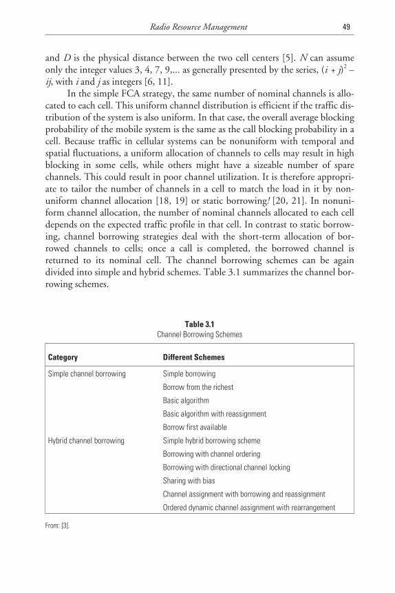
and D is the physical distance between the two cell centers [5]. N can assumeonly the integer values 3, 4, 7, 9,... as generally presented by the series, (i + j)2 –ij, with i and j as integers [6, 11].

In the simple FCA strategy, the same number of nominal channels is allo-cated to each cell. This uniform channel distribution is efficient if the traffic dis-tribution of the system is also uniform. In that case, the overall average blockingprobability of the mobile system is the same as the call blocking probability in acell. Because traffic in cellular systems can be nonuniform with temporal andspatial fluctuations, a uniform allocation of channels to cells may result in highblocking in some cells, while others might have a sizeable number of sparechannels. This could result in poor channel utilization. It is therefore appropri-ate to tailor the number of channels in a cell to match the load in it by non-uniform channel allocation [18, 19] or static borrowing! [20, 21]. In nonuni-form channel allocation, the number of nominal channels allocated to each celldepends on the expected traffic profile in that cell. In contrast to static borrow-ing, channel borrowing strategies deal with the short-term allocation of bor-rowed channels to cells; once a call is completed, the borrowed channel isreturned to its nominal cell. The channel borrowing schemes can be againdivided into simple and hybrid schemes. Table 3.1 summarizes the channel bor-rowing schemes.


Table 3.1Channel Borrowing Schemes

Category Different Schemes

Simple channel borrowing Simple borrowing

Borrow from the richest

Basic algorithm

Basic algorithm with reassignment

Borrow first available

Hybrid channel borrowing Simple hybrid borrowing scheme

Borrowing with channel ordering

Borrowing with directional channel locking

Sharing with bias

Channel assignment with borrowing and reassignment

Ordered dynamic channel assignment with rearrangement

From: [3].

3.3.3.2 DCA

Due to short-term temporal and spatial variations of traffic in cellular systems,FCA schemes are not able to attain high channel efficiency. To overcome this,DCA schemes have been studied during the past twenty years. In contrastto FCA, there is no fixed relationship between channels and cells in DCA. Allchannels are kept in a central pool and are assigned dynamically to radio cells asnew calls arrive in the system [22, 23]. After a call is completed, its channel isreturned to the central pool. In DCA, a channel is eligible for use in any cell pro-vided that signal interference constraints are satisfied.

Because, in general, more than one channel might be available in the cen-tral pool to be assigned to a cell that requires a channel, some strategy must beapplied to select the assigned channel [15]. The main idea of all DCA schemes isto evaluate the cost of using each candidate channel and to select the one withthe minimum cost provided that certain interference constraints are satisfied.The selection of the cost function is what differentiates DCA schemes [15]. Theselected cost function might depend on the future blocking probability in thevicinity of the cell, the usage frequency of the candidate channel, the reuse dis-tance, channel occupancy distribution under current traffic conditions, radiochannel measurements of individual mobile users, or the average blocking prob-ability of the system [7]. Table 3.2 gives a list of the proposed DCA schemes.

3.3.4 Transmitter Power Control

Power control is another supplementary technique to handle RRM. Power con-trol can serve various purposes:

• To suppress adjacent channel (cross-correlation) interference in nonor-thogonal schemes;

• To minimize power consumption in order to extend terminal batterylife;

• To control cochannel interference (in schemes with orthogonal wave-forms).

As discussed in the previous section, the purpose of CA algorithms is toassign radio channels to mobile users such that a certain level of CIR is main-tained at every MT. Hence, one can also use power control schemes to achievethe desired CIR level. This is why the selection of the proper transmitter powerin MTs and BSs is another important issue that has attracted considerable atten-tion in recent years.

In the resource allocation problem context, it can be shown that the maxi-mum number of terminals is supported under a power control regime that


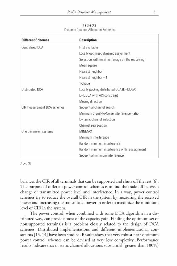
balances the CIR of all terminals that can be supported and shuts off the rest [6].The purpose of different power control schemes is to find the trade-off betweenchange of transmitted power level and interference. In a way, power controlschemes try to reduce the overall CIR in the system by measuring the receivedpower and increasing the transmitted power in order to maximize the minimumlevel of CIR in the system.

The power control, when combined with some DCA algorithm in a dis-tributed way, can provide most of the capacity gain. Finding the optimum set ofnonsupported terminals is a problem closely related to the design of DCAschemes. Distributed implementations and different implementational con-straints [13, 14] have been studied. Results show that very robust near-optimumpower control schemes can be devised at very low complexity. Performanceresults indicate that in static channel allocations substantial (greater than 100%)


Table 3.2Dynamic Channel Allocation Schemes

Different Schemes Description

Centralized DCA First available

Locally optimized dynamic assignment

Selection with maximum usage on the reuse ring

Mean square

Nearest neighbor

Nearest neighbor + 1

1-clique

Distributed DCA Locally packing distributed DCA (LP-DDCA)

LP-DDCA with ACI constraint

Moving direction

CIR measurement DCA schemes Sequential channel search

Minimum Signal-to-Noise Interference Ratio

Dynamic channel selection

Channel segregation

One dimension systems MINMAX

Minimum interference

Random minimum interference

Random minimum interference with reassignment

Sequential minimum interference

From: [3].

capacity gains can be achieved using optimum power control. These gains are, ofcourse, not additive with the gains obtained by DCA schemes. Preliminaryresults, however, regarding DCA combined with power control schemes showsubstantial capacity gains [15, 17].

3.4 Handoff Process

An issue that is closely related to CA techniques is the handoff mechanism,which is usually associated with the movement of MTs. Handoff is defined asthe change of radio channel used by a MT. Handoff management enables thenetwork to maintain a user’s connection as the mobile terminal continues tomove and change its access point to the network. This is performed in threesteps: initiation, connection generation, and data flow control.

The cause of handoff may be poor radio quality due to a change in theenvironment or the movement of the MT. As MTs move about in the servicearea, the propagation and interference situation may change such that the samecell (or BS) on any waveform cannot support the terminal. In addition, newMTs may enter the service area requiring services, while others terminate theircommunication sessions. Since most of the basic resource allocation strategiesdeal mainly with static situations encountered on a short-term timescale,resource management schemes should be capable of handling these variations.In general, the handoff event is caused by the radio link degradation or is initi-ated by the system that rearranges radio channels in order to avoid congestion.Handoff is extremely important in any mobile network because of the cellulararchitecture employed to maximize spectrum utilization. Handoff can be classi-fied into network-controlled (or hard) handoff, and mobile-controlled (or soft)handoff. We shall discuss them now.

3.4.1 Network-Controlled Handoff (Hard Handoff)

In network-controlled handoff, when a mobile user moves to the edge of the cellboundary, the network invokes the handoff process. Since it is either all or noth-ing, the transition is a “hard” one. The user experiences an interruption causedby frequency shifting. Handoff initiation occurs dependent on different criteriaand strategies used. The most common criteria are (1) relative signal strength,(2) relative signal strength with threshold, (3) relative signal strength withhysteresis, and (4) relative signal strength with hysteresis and threshold (seeFigure 3.3).

Hard handoff may be intracell or intercell, depending upon whether thenew radio channel is with the same BS (intracell handoff) or with a new BS(intercell handoff). In the first case, it is a waveform reallocation within the same


TEAMFLY

Team-Fly®

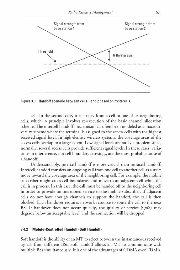
cell. In the second case, it is a relay from a cell to one of its neighboringcells, which in principle involves re-execution of the basic channel allocationscheme. The intercell handoff mechanism has often been modeled as a macrodi-versity scheme where the terminal is assigned to the access cells with the highestreceived signal level. In high-density wireless systems, the coverage areas of theaccess cells overlap to a large extent. Low signal levels are rarely a problem since,normally, several access cells provide sufficient signal levels. In these cases, varia-tions in interference, not cell boundary crossings, are the most probable cause ofa handoff.

Understandably, intercell handoff is more crucial than intracell handoff.Intercell handoff transfers an ongoing call from one cell to another cell as a usersmove toward the coverage area of the neighboring cell. For example, the mobilesubscriber might cross cell boundaries and move to an adjacent cell while thecall is in process. In this case, the call must be handed off to the neighboring cellin order to provide uninterrupted service to the mobile subscriber. If adjacentcells do not have enough channels to support the handoff, the call is thenblocked. Each handover requires network resource to route the call to the nextBS. If handover does not occur quickly, the quality of service (QoS) maydegrade below an acceptable level, and the connection will be dropped.

3.4.2 Mobile-Controlled Handoff (Soft Handoff)

Soft handoff is the ability of an MT to select between the instantaneous receivedsignals from different BSs. Soft handoff allows an MT to communicate withmultiple BSs simultaneously. It is one of the advantages of CDMA over TDMA.


H (hysteresis)

Signal strength frombase station 1

Signal strength frombase station 2

Threshold

Figure 3.3 Handoff scenario between cells 1 and 2 based on hysteresis.

Soft handoff is an effective way to increase the capacity, reliability, and coveragerange of CDMA systems.

In TDMA or Advanced Mobile Phone System (AMPS), due to spectrumreuse, a given slot on a given frequency channel cannot be used by neighboringcells. So when an MT that is in a call moves from one cell to another, at a certainpoint it has to switch between cells. In AMPS and TDMA, it will be com-manded by the system to change frequencies all at once (hard handoff, as dis-cussed above). On the contrary, in CDMA, all the cells operate on the samefrequency. The MT still has a single RF receiver, which converts RF down tobaseband, but behind that it has a rake receiver with multiple fingers. Since allthe cells operate on the same frequency, the single RF receiver picks up all ofthose that are within range. The MT then assigns fingers from the rake receiverto various signals, and these are added together to create the full signal that theMT utilizes. Sometimes these are multiple paths from the same cell. Forinstance, if there is a direct route from the cell to the MT, and in addition thesignal travels to a large building and reflects off it before reaching the MT, thenthe MT can utilize both of these signals for additional clarity. We have alreadydiscussed this as a multipath phenomenon, in Section 3.1, which essentiallydegrades TDMA and AMPS performance. But soft handoff is even more usefulwhen the MT is about halfway between two cells. While in a call, the MT is notonly handling the transport of data back and forth to the cell, but it is alsoactively looking for other cells. When the MT finds a cell with good signalstrength (on the same frequency, remember) it will inform the cell system. Thecell system might decide, at that point, to route the call through both cellssimultaneously. The specification actually permits an MT to talk to six cells atonce, though no MT currently in existence has this capability.

There are two key requirements for realizing soft handoff:

1. Data distribution and selection: Separate copies of the same data need tobe sent via multiple BSs to the same MT (or in the reverse direction,from an MT to multiple BSs).

2. Data content synchronization: Pieces of data arriving from multipleBSs to an MT at the same time should be copies of the same data inorder for the MT’s radio system to correctly combine these copiesinto a single copy. In the reverse direction, only one copy of the datasent by the MT to multiple BSs should be selected for delivery to thedestination.

So when a CDMA phone in a call moves from one cell to another, thehandoff process happens in multiple steps. First the phone notices the secondcell, and the cell system begins to carry the call on both cells. As the phone con-tinues to move, eventually the signal strength from the cell the phone is moving


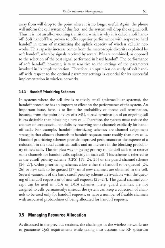
away from will drop to the point where it is no longer useful. Again, the phonewill inform the cell system of this fact, and the system will drop the original cell.Thus it is not an all-or-nothing transition, which is why it is called a soft hand-off. Soft handoff has proven to offer superior performance with respect to hardhandoff in terms of maximizing the uplink capacity of wireless cellular net-works. This capacity increase comes from the macroscopic diversity exploited bysoft handoff, whereby signals received by several BSs are combined, as opposedto the selection of the best signal performed in hard handoff. The performanceof soft handoff, however, is very sensitive to the settings of the parametersinvolved in its implementation. Therefore, an optimization study of soft hand-off with respect to the optimal parameter settings is essential for its successfulimplementation in wireless networks.

3.4.3 Handoff Prioritizing Schemes

In systems where the cell size is relatively small (microcellular systems), thehandoff procedure has an important effect on the performance of the system. Animportant issue, here, is to limit the probability of forced call termination,because, from the point of view of a MU, forced termination of an ongoing callis less desirable than blocking a new call. Therefore, the system must reduce thechances of unsuccessful handoffs by reserving some channels explicitly for hand-off calls. For example, handoff prioritizing schemes are channel assignmentstrategies that allocate channels to handoff requests more readily than new calls.Handoff prioritizing schemes provide improved performance at the expense of areduction in the total admitted traffic and an increase in the blocking probabil-ity of new calls. The simplest way of giving priority to handoff calls is to reservesome channels for handoff calls explicitly in each cell. This scheme is referred toas the cutoff priority scheme (CPS) [19, 24, 25] or the guard channel scheme[26, 27]. Other prioritizing schemes allow either the handoff to be queued [24,26] or new calls to be queued [27] until new channels are obtained in the cell.Several variations of the basic cutoff priority scheme are available with the queu-ing of handoff requests or of new call requests [25–27]. The guard channel con-cept can be used in FCA or DCA schemes. Here, guard channels are notassigned to cells permanently; instead, the system can keep a collection of chan-nels to be used only for handoff requests, or have a number of flexible channelswith associated probabilities of being allocated for handoff requests.

3.5 Managing Resource Allocation

As discussed in the previous sections, the challenges in the wireless networks areto guarantee QoS requirements while taking into account the RF spectrum


limitations and radio propagation impairments. As the demand for wireless serv-ice increases, managing radio resource becomes more complicated. Figure 3.4depicts the generic functional blocks used for RRM in a typical cellular system.This shows that CA strategy has to be supported by handoff strategy, powercontrol, and call admission control (CAC) in order to entail a balanced RRM.We have already discussed CA, handoff, and power control above. Here we willdwell on CAC and QoS issues to complement our earlier discussions.

3.5.1 CAC

CAC denotes the process of making a decision for every new call admissionaccording to the amount of available resource versus users’ QoS requirements,and the effect upon the QoS of the existing calls imposed by each new call.Whenever a new MT (either a new request for service or an intercell handoff)arrives in a BS, the RRM system has to decide if this particular MT may beallowed into the system. An algorithm making these decisions is called a CACalgorithm. Since the precise MT population and gain matrix may not be trackedexactly at all times, and due to the complexity of RRM algorithms, determiningthe success of an admission decision may not be possible beforehand withoutphysically executing the admission itself. CAC can be divided into two groups,


Channelassignmentstrategy

Calladmissioncontrol

Handoffstrategy

Powercontrol

Multipleaccesssystem

Cell

Figure 3.4 Generic function blocks of CAC.

interference-based CAC and user-based CAC. In interference-based algorithms,admission control is based on the CIR parameter, while user-based algorithmsare dependent on the number of channels available.

Traditional approaches involving static channel allocation normally usesimple thresholding strategies on the available channels in each cell. This tradi-tional CAC algorithm is known as the guard channel algorithm. The guardchannel is a concept based on reserving a fraction of channels for the purpose ofhandoff by considering only the status for a local cell. Here, BSs are assigned afixed set of channels that provide a certain low-outage probability. Such a sys-tem is called blocking-limited. Whenever a call arrives, the system checkswhether or not there are channels available. New arriving calls are admitted upto the point at which there is only some small fraction of the resource remain-ing. This spare capacity is reserved for calls entering a cell due to an intercellhandoff.

In systems using dynamic channel allocation or random allocation, there isno clear limit on the number of channels or waveforms that can be used. In suchinterference-limited systems, the feasibility of admitting new users will dependon the current interference situation. This is particularly complicated in systemsutilizing CIR-balancing power control by the fact that terminals already activewill react to the admission of a new terminal by adjusting (raising) their trans-mitter powers. When several access cells provide sufficient CIR, the system isalso able to handle traffic variations by means of load sharing. However, provid-ing guaranteed service (in terms of continuity in channels) to the MTs in a large(possibly global) wireless system, coupled with mobility management, is a for-midable task indeed.

There are also some nontraditional methods that have been proposedrecently. They are based on adaptive techniques, where channels are allocatedand reserved in a dynamic way using teletraffic analysis, prediction of injectedtraffic, and prediction of MT movement. In some prediction schemes, it issufficient to take care of the radio resource that the mobile will need in thepredicted location. In general, the resource reservation mechanism consistsof two parts: some of the bandwidth reserved in the next cell the mobile is likelyto visit, and a common pool of dynamically adjusted bandwidth used to accom-modate other unpredicted flows. The next cell is predicted based on the mobil-ity pattern observed in various cells. An approach that utilizes reservation ofbandwidth along the predicted path of the mobile, or along some neighborsofNthat path, is based on the concept of shadow clustering. The fundamentalidea of the shadow-cluster concept is that, as an active MT travels to anothercell, the region of influence also moves, following the active MT to its newlocation. The BSs currently being influenced are said to form a shadow cluster,because the region of influence follows the movement of the active MT like ashadow.


Other similar approaches include schemes that rely on the extended loca-tion information (from adjacent cells) to make the CAC decision. The band-width reservation could be estimated based upon the history of the nominal celland neighboring cells. The queuing of new calls and handover requests isanother approach that reduces the blocking probability and probability offorced termination. There is a trade-off between the increase in service qualityand the corresponding decrease in total carried traffic. The queuing of a handoffrequest is more sensitive to delay in service than the queuing of a new call, lead-ing to queuing of new calls rather than handoff calls. One of the key points ofusing queuing in CAC is that service differentiation can be managed with modi-fied queuing disciplines. Instead of a first in–first out (FIFO) queuing strategy,other prioritized queuing disciplines can be used to maintain priority levels ineach service class.

3.5.2 QoS

As we move towards the next-generation mobile systems, the need for improv-ing coverage, system capacity, and service quality becomes more and moreimportant. Different service classes have different QoS requirements. Futureservices will also have widely varying QoS requirements. The network must beable to handle these requirements in order to satisfy end users without wastingnetwork resources. Moreover, to have any meaning, QoS provisioning must beend-to-end (i.e. from service to terminal). The radio interface is the scarcestresource in the mobile network and is a rather hostile environment, beingerror-prone and subject to radio propagation conditions that can vary over time.Consequently, effective QoS management in the radio network layer of themobile network is a must. RRM will be the major differentiator between theoverall QoS provisioning offered by different operators’ networks.

To satisfy these requirements, the network must have enough capacity toserve arriving calls and flexible mechanisms to guarantee certain services. Con-nections are allocated to the system and cell layer that provide the requestedQoS for the requested service most effectively. In this way, network resourcesare not wasted providing excess QoS to those services that do not require it,while higher quality resources are reserved for those services that require them.Within each system, the radio parameters will be set according to the QoSrequirements of the radio service. These include the selection of channel, codingrate, and retransmission scheme for example. Conventionally, in a single layersystem, reserving a number of channels in advance, known as guard channels,often does support prioritized handoff. Allocation of channels can either bedynamic or static, depending on the traffic pattern. Queuing is another methodfavoring handoff calls. By queuing new call arrivals, available bandwidth can bededicated to handoff calls.


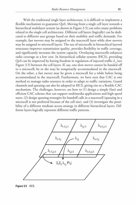
With the traditional single layer architecture, it is difficult to implement aflexible mechanism to guarantee QoS. Moving from a single cell layer towards ahierarchical multilayer system (as shown in Figure 3.5) can solve many problemsrelated to the single cell architecture. Different cell layers (logically) can be dedi-cated to different user groups based on their mobility and traffic demands. Forexample, fast movers may be assigned to the macrocell layer while slow moversmay be assigned to microcell layers. The use of microcells in hierarchical layeredstructures improves transmission quality, provides flexibility in traffic coverage,and significantly increases the system capacity. Overlaying macrocells enhancesradio coverage at a low cost. In hierarchical cellular systems (HCS), providingQoS can be improved by having freedom in regulation of injected traffic λ ij (seeFigure 3.5) between the cell layers. If, say, one slow mover cannot be handed offto a microcell, he or she may be temporarily accommodated in the macrocell.On the other, a fast mover may be given a microcell for a while before beingaccommodated in the macrocell. Furthermore, we have seen that CAC is onemethod to manage radio resource in order to adapt to traffic variations. Guardchannels and queuing can also be adopted in HCS, giving rise to a flexible CACmechanism. The challenges, however, are how to (1) design a simple (fast) andefficient CAC scheme that can support multimedia applications and high-speedusers, (2) design queuing strategies for handoff calls in a macrocell (queuing in amicrocell is not preferred because of the cell size), and (3) investigate the possi-bility of a different medium access strategy in different hierarchical layers. Dif-ferent layers logically represent different traffic patterns.


λi-1,j-1 λi,j-1 λi+1,j-1

λi-1,j λi,j λi+1,j

λi-1,j+1 λi,j+1 λi+1,j+1

ΣΣ λi j i,j Pi,j

Figure 3.5 HCS.

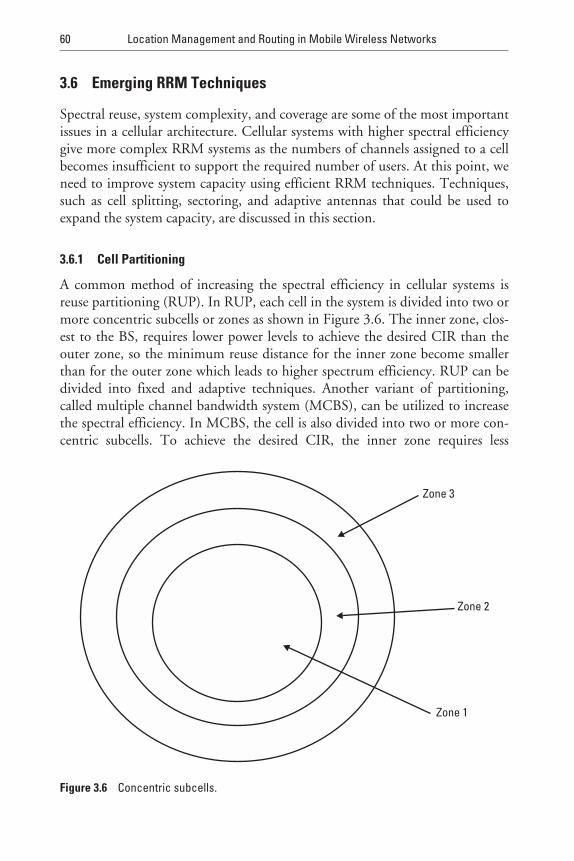
3.6 Emerging RRM Techniques

Spectral reuse, system complexity, and coverage are some of the most importantissues in a cellular architecture. Cellular systems with higher spectral efficiencygive more complex RRM systems as the numbers of channels assigned to a cellbecomes insufficient to support the required number of users. At this point, weneed to improve system capacity using efficient RRM techniques. Techniques,such as cell splitting, sectoring, and adaptive antennas that could be used toexpand the system capacity, are discussed in this section.

3.6.1 Cell Partitioning

A common method of increasing the spectral efficiency in cellular systems isreuse partitioning (RUP). In RUP, each cell in the system is divided into two ormore concentric subcells or zones as shown in Figure 3.6. The inner zone, clos-est to the BS, requires lower power levels to achieve the desired CIR than theouter zone, so the minimum reuse distance for the inner zone become smallerthan for the outer zone which leads to higher spectrum efficiency. RUP can bedivided into fixed and adaptive techniques. Another variant of partitioning,called multiple channel bandwidth system (MCBS), can be utilized to increasethe spectral efficiency. In MCBS, the cell is also divided into two or more con-centric subcells. To achieve the desired CIR, the inner zone requires less


Zone 1

Zone 2

Zone 3

Figure 3.6 Concentric subcells.

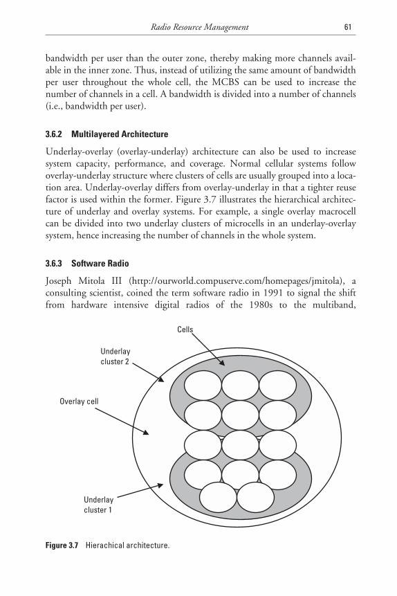
bandwidth per user than the outer zone, thereby making more channels avail-able in the inner zone. Thus, instead of utilizing the same amount of bandwidthper user throughout the whole cell, the MCBS can be used to increase thenumber of channels in a cell. A bandwidth is divided into a number of channels(i.e., bandwidth per user).

3.6.2 Multilayered Architecture

Underlay-overlay (overlay-underlay) architecture can also be used to increasesystem capacity, performance, and coverage. Normal cellular systems followoverlay-underlay structure where clusters of cells are usually grouped into a loca-tion area. Underlay-overlay differs from overlay-underlay in that a tighter reusefactor is used within the former. Figure 3.7 illustrates the hierarchical architec-ture of underlay and overlay systems. For example, a single overlay macrocellcan be divided into two underlay clusters of microcells in an underlay-overlaysystem, hence increasing the number of channels in the whole system.

3.6.3 Software Radio

Joseph Mitola III (http://ourworld.compuserve.com/homepages/jmitola), aconsulting scientist, coined the term software radio in 1991 to signal the shiftfrom hardware intensive digital radios of the 1980s to the multiband,


Overlay cell

Underlaycluster 2

Underlaycluster 1

Cells

Figure 3.7 Hierachical architecture.

multimode, software-defined radios of 2000 and beyond. According to him, inthe future, software radio will give an MT many different radio access interfaceswithout increasing the terminal complexity or cost.

As described in Chapter 1, radio network architectures have alreadyevolved from early point-to-point and relatively chaotic peer networks (e.g.,push-to-talk mobile military radio networks) toward more hierarchical struc-tures with improved service quality (Cellular and PCS networks). In addition,channel data rates continue to increase through multiplexing and spectrumspreading. As communications technology continues its rapid transition fromanalog to digital, more functions of contemporary radio systems are imple-mented in software—leading toward software radio [28]. With software radiotechnology, MTs can access different networks according to their services. In amultiple-hierarchy application, a single radio unit, typically an MT, participatesin more than one network hierarchy. A software radio terminal could, for exam-ple, operate in a GSM-based PCS network, an AMPS network, and a future sat-ellite mobile network.

Technically speaking, a software radio is a radio whose channel modula-tion waveforms are defined in software. That is, waveforms are generated assampled digital signals, converted from digital to analog via a wideband digitalto analog converter (DAC) and then possibly upconverted from intermediatefrequency (IF) to RF. The receiver, similarly, employs a wideband analog todigital converter that captures all of the channels of the software radio node. Thereceiver then extracts, downconverts and demodulates the channel waveformusing software on a general-purpose processor. Software radios employ a combi-nation of techniques that include multiband antennas and RF conversion; wide-band ADC and digital to analog conversion, and the implementation of IF,baseband, and bitstream processing functions in general-purpose programmableprocessors. The resulting software radio, or software-defined radio (SDR), inpart extends the evolution of programmable hardware, increasing flexibility viaincreased programmability. And in part it represents an ideal that may never befully implemented but that nevertheless simplifies and illuminates trade-offs inradio architectures that seek to balance standards compatibility, technologyinsertion, and the compelling economics of today’s highly competitive market-places. It is pertinent to mention here that there is a worldwide SDR Forum(http://www.sdrforum.org), which is an open, nonprofit corporation dedicatedto supporting the development, deployment, and use of open architectures foradvanced wireless systems. The Forum membership is international and is grow-ing enormously.

The use of a software radio that can program a specific waveform for use indifferent wireless settings will make it possible to adapt the link to changing con-ditions. Such an approach is also expected to facilitate the management of QoS.In a region with many different independent radio access networks, one cannot


TEAMFLY

Team-Fly®

explore the optimal use of available frequency resource and distribution of userswithin different radio access networks as one can in a centralized system. Theidea is to integrate different distributed radio access networks to a centralizednetwork architecture. With a centralized system, we can gain increasing trunk-ing capacity and QoS in the region. The terminal reconfigurability provided bySDR technology introduces flexibility in spectrum management when differentheterogeneous radio systems exist in the same geographical area. Consideringdevelopment of and experimentation with wireless multimedia to be of greatimportance, initiatives in this area would be extremely useful. Development ofsuch a software radio would help develop commercial products that can handleseveral services (e.g., AMPS, DAMPS, GSM, PCS, CDMA) in a single region.Trying out new schemes and ideas would also consume very little time with soft-ware radio. Software radio is now being enhanced to produce cognitive radio, anemerging topic within software radio. It refers to that class of software radio thatemploys model-based reasoning and at least a chess-program level of sophistica-tion in using, planning, and creating radio etiquettes.

3.7 Integrated RRM

Future mobile networks will not consist simply of one radio access technology,such as WCDMA or EDGE, but will contain several different technologies asshown in Figure 3.1. The structure of operators’ networks is becoming morecomplex, including multiple radio technologies in hierarchical cell structures;macrocell, microcell, and picocell layers. It is even possible that the same radiotechnology will be deployed on several different frequency bands. Simply speak-ing, the future is a hybrid (multiradio) environment. This will allow the net-works to benefit from the individual coverage and capacity characteristics ofeach one, resulting in the most economic solution with the highest levels of serv-ice. In such a network, a multimode terminal will have the possibility of using awide range of different resources. The motivation for hybrid networks arisesfrom the fact that no one technology or service can provide ubiquitous coverage,and it will be necessary for an MT to employ attachment to different networksto maintain connection during the service time.

The emergence of a variety of mobile data services with variable coverage,bandwidth, and handoff strategies has attracted tremendous attention to theneed for roaming among different radio access networks in a hybrid networkarchitecture. The capabilities of network operators6 current infrastructure canbe evolved and form part of this multiradio hybrid network, maximizing theusage of existing network investments. For this vision to work, these differenttechnologies must be seamlessly integrated to form a single access network sothat the end user will be unaware of the access technology being used. Similarly,


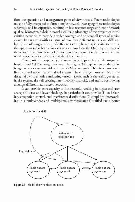
from the operation and management point of view, these different technologiesmust be fully integrated to form a single network. Managing these technologiesseparately will be expensive, resulting in low resource usage and poor networkquality. Moreover, hybrid networks will take advantage of the properties in theexisting networks to provide a wider coverage and to serve all types of serviceclasses. In a network with a mixture of resources (different systems and differentlayers) and offering a mixture of different services, however, it is vital to providethe optimum radio bearer for each service, based on the QoS requirements ofthe service. Overprovisioning QoS to those services or users that do not requireit will waste network resources and should be avoided.

One solution to exploit hybrid networks is to provide a single integratedhandoff and CAC strategy. For example, Figure 3.8 depicts the model of anintegrated access system with a virtual RRM access node. This virtual node actslike a control node in a centralized system. The challenge, however, lies in thedesign of a virtual node considering various factors, such as the traffic generatedin the system, the cell crossing rate (mobility analysis), and traffic overflowingamongst different radio access networks.

It can provide extra capacity to the network, resulting in higher end-useraverage bit rates and lower blocking. In particular, it can provide (1) load shar-ing, congestion control, and interference distribution; (2) simplified interwork-ing in a multivendor and multisystem environment; (3) unified radio bearer


Physical flow

Admission handoff

Virtual radioaccess node

Radio accesssystem 1

Radio accesssystem 2

Radio accesssystem m

Figure 3.8 Model of a virtual access node.

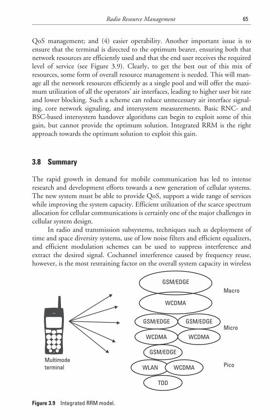
QoS management; and (4) easier operability. Another important issue is toensure that the terminal is directed to the optimum bearer, ensuring both thatnetwork resources are efficiently used and that the end user receives the requiredlevel of service (see Figure 3.9). Clearly, to get the best out of this mix ofresources, some form of overall resource management is needed. This will man-age all the network resources efficiently as a single pool and will offer the maxi-mum utilization of all the operators’ air interfaces, leading to higher user bit rateand lower blocking. Such a scheme can reduce unnecessary air interface signal-ing, core network signaling, and intersystem measurements. Basic RNC- andBSC-based intersystem handover algorithms can begin to exploit some of thisgain, but cannot provide the optimum solution. Integrated RRM is the rightapproach towards the optimum solution to exploit this gain.

3.8 Summary

The rapid growth in demand for mobile communication has led to intenseresearch and development efforts towards a new generation of cellular systems.The new system must be able to provide QoS, support a wide range of serviceswhile improving the system capacity. Efficient utilization of the scarce spectrumallocation for cellular communications is certainly one of the major challenges incellular system design.

In radio and transmission subsystems, techniques such as deployment oftime and space diversity systems, use of low noise filters and efficient equalizers,and efficient modulation schemes can be used to suppress interference andextract the desired signal. Cochannel interference caused by frequency reuse,however, is the most restraining factor on the overall system capacity in wireless


Micro

WLAN

GSM/EDGE

WCDMA

GSM/EDGE GSM/EDGE

WCDMAWCDMA

GSM/EDGE

WCDMA

TDD

Macro

PicoMultimodeterminal

Figure 3.9 Integrated RRM model.

networks, and the main idea behind channel assignment strategies is to make useof radio propagation path-loss characteristics in order to minimize the CIR andhence increase the radio spectrum reuse efficiency.

In conclusion, a few remarks follow regarding what we believe to be futuretrends in radio resource allocation. Wideband and mixed rate traffic in small cellenvironments will exhibit a very large peak to average capacity demands. DCA(statistical multiplexing) will provide even larger capacity gains in these situa-tions. Conventional single cell traffic multiplexing and averaging will surely notbe sufficient, making dynamic spatial resource reuse of paramount importance[8]. Small cell systems allow greater spectral reuse and larger capacity, butinduce an increasing number of handoffs, while overlaying cells provide cover-age and service for high-speed users. Hierarchical cell architectures can thereforeserve all types of user classes with different services and speed. The system per-formance characteristics include blocking probability, handoff blocking prob-ability, forced termination of ongoing calls, and total carried traffic.

Traditionally we consider the frequency spectrum to be the resource to beshared. Since theoretically, there does not exist any upper limit on the capacitythat can be provided (with a dense enough infrastructure), it is important thatwe widen the resource management perspective. Parameters such as infrastruc-ture density costs and terminal power consumption play important roles. Onecould easily identify trade-offs such as where the signal-processing load shouldbe put in a wireless system—in the terminal where power is scarce or in the fixedinfrastructure. The key question here is: Should the access port (cell) infrastruc-ture be very dense (and costly) allowing for “dumb,” cheap, low-power termi-nals or should terminals be more complex allowing for the rapid deployment ofa cheap infrastructure at the expense of battery life and terminal cost?

Future systems are expected to require much higher data rates than currentsystems. In third-generation wide-area personal communication systems (suchas UMTS and FPLMTS) data rates in the range of 64 Kbps to 2 Mbps are com-ing [8]. Since the required transmitter power increases linearly with the band-width, high-speed radio access will have only a very limited range. This clearlyhas repercussions on the economics of such systems: either the investment willhave to be heavy in a dense ubiquitous infrastructure, or be limited to coveringonly certain areas where users will require extensive bandwidth requirements.The design and performance of RRM algorithms is not affected much by theincrease in bandwidth per se. In fact, much of the on-air signaling required bymany of the adaptive schemes will, relatively speaking, occupy a smaller fractionof the available bandwidth. Increasing the infrastructure density with more BSswill clearly cause an increase in complexity in the RRM algorithms.

CDMA has been widely accepted as the major multiple access scheme inthird-generation mobile communication systems [8]. WCDMA and its hybridassociate time-division CDMA are key elements of the IMT-2000 framework


of standards. Since the beginning of the 1990s, there has been enormousresearch activity in analysis of the soft (i.e., interference-limited) capacity ofthese CDMA-based systems. Optimal usage of the soft capacity to provide,maintain, and guarantee QoS for different service classes is now becoming a veryimportant issue. Therefore, interest in radio resource allocation has recentlyincreased. RRM schemes (primarily for CDMA-based systems) should be flexi-ble, support traffic services with various QoS requirements, minimize call or ses-sion blocking and dropping probabilities, and have acceptable radio resourceutilization.

References

[1] Neskovic A., N. Neskovic, and G. Paunovic, “Modern Approaches in Modeling of MobileRadio Systems Propagation Environment,” IEEE Communications Survey, Third Quarter,2000.

[2] Lopez, A. R., “Application of Wedge Diffraction Theory to Estimating Power Density atAirport Humped Runway,” IEEE Trans. on Antennas and Propagation, June 1987,pp. 689–714.

[3] Katzela, I., and M. Naghshineh, “Channel Assignment Schemes for Cellular Mobile Tele-communication Systems: A Comprehensive Survey,” IEEE Personal Communication, June1996, pp. 10–31.

[4] Zander, J., “Radio Resource Management in Future Wireless Networks: Requirementsand Limitations,” IEEE Communications Magazine, Aug. 1997, pp. 30–96.

[5] Lee, W. C. Y., “New Cellular Schemes for Spectral Efficiency,” IEEE Trans. on VehicularTechnology, 1987, pp. 188–192.

[6] Lee, W. C. Y., Mobile Cellular Communication Systems, 1989.

[7] Tekinay, S., and B. Jabbari, “Handover and Channel Assignment in Mobile Cellular Net-works,” IEEE Communications Magazine, 1991.

[8] Jorguseski, L., J. Farserotu, and R. Prasad, “Radio Resource Allocation in Third-Generation Mobile Communication Systems,” IEEE Communications Magazine, Feb.2001, pp. 117–123.

[9] Zander, J. “Asymptotic Bounds on the Performance of a Class of Dynamic ChannelAssignment Algorithms,” IEEE JSAC, 1993, pp. 926–933.

[10] Chuang, J .C. I., “Performance Issues and Algorithms for Dynamic Channel Assignment,”IEEE JSAC, 1993.

[11] Kahwa, T. J., and N. Georganas, “A Hybrid Channel Assignment Scheme in Large ScaleCellular-Structured Mobile Communication Systems,” IEEE Trans. on Communication,1978, pp. 432–438.


[12] Sin, J., and N. Georganas, “A Simulation Study of a Hybrid Channel Assignment Schemefor Cellular Land-Mobile Radio Systems with Erlang-C Service,” IEEE Trans. on Commu-nication, 1981, pp. 143–147.

[13] Cox, D., and D. O. Reudink, “Increasing Channel Occupancy in Large-Scale MobileRadio Systems: Dynamic Channel Reassignment,” IEEE Trans. on Vehicular Technology,1973, pp. 218–222.

[14] Cox, D., and D. O. Reudink, “A Comparison of Some Non-Uniform Spatial DemandProfiles on Mobile Radio System Performance,” IEEE Trans. on Communication, 1972,pp. 190–195.

[15] Cox, D., and D. O. Reudink, “Dynamic Channel Assignment in Two Dimension Large-Scale Mobile Radio Systems,” Bell Sys. Tech. J., Vol. 51, 1972, pp. 1611–1628.

[16] Schiff, L. “Traffic Capacity of Three Types of Common User Radio Communication Sys-tems,” IEEE Trans. on Communication Tech., 1970, pp. 12–21.

[17] Jakes, W. C., Jr., Microwave Mobile Communications, New York: Wiley, 1974.

[18] Zhang, M., and T. S. Yum, “The Non-Uniform Compact Pattern Allocation Algorithmfor Cellular Mobile Systems,” IEEE Trans. on Vehicular Tech., 1991, pp. 387–391.

[19] Oh, S. H., et al., “Prioritized Channel Assignment in a Cellular Radio Network,” IEEETrans. on Communication, 1992, pp. 1259–69.

[20] Anderson, L., “A Simulation Study of Dynamic Channel Assignment Algorithms in HighCapacity Mobile Telecommunications System,” IEEE Trans. on Vehicular Tech., 1973.

[21] Engel, J. S., and M. Peritsky, “Statistically Optimum Dynamic Server Assignment in Sys-tems with Interfering Servers,” IEEE Trans. on Vehicular Tech., Vol. VT-22, 1973,pp. 203–209.

[22] Okada, K., and F. Kubota, “On Dynamic Channel Assignment Strategies in CellularMobile Radio Systems,” IEICE Trans. Fundamentals, 1992, pp. 1634–1641.

[23] Okada, K., and F. Kubota, “On Dynamic Channel Assignment in Cellular Mobile RadioSystems,” Proc. IEEE Int. Symp. on Circuits and Systems, 1991, pp. 938–941.

[24] Hong, D., and S. Rappaport, “Traffic Modeling and Performance Analysis for CellularMobile Radio Telephone Systems with Prioritized and Nonprioritized Handoff Proce-dures,” IEEE Trans. on Vehicular Tech., 1986, pp. 77–92.

[25] Tekinay, S., “A Measurement-Based Prioritization Scheme for Handovers in Mobile Cel-lular Networks,” IEEE JSAC, Vol. 1, 1992, pp. 1343–1350.

[26] Posner, C., and R. Guerin, “Traffic Policies in Cellular Radio that Minimize Blocking ofHandoffs,” ITC-II, 1985, pp. 2.4B.2.1–2.4B.2.5.

[27] Guerin, R., “Queuing Blocking System with Two Arrival Streams and Guard Channels,”IEEE Trans. on Communication, 1988, pp. 153–163.

[28] Burns, P., Software Radio Systems Design, Norwood, MA: Artech House, 2002.


4Location Management

Portable computers and communication devices with wireless connection to thenetwork are changing the way people think about and use computing and com-munication. These wireless devices can communicate with each other eventhough the user is mobile. People carrying a mobile computer will, therefore, beable to access information regardless of time and current position. For example,they will be able to receive and send e-mail from any location or receive currentinformation about local traffic, bus, and train services. But, location manage-ment will be an important problem in these situations because wireless devicescan change location while connected to the network. New strategies must beintroduced to deal with the dynamic changes of a mobile device’s networkaddress. A detailed description of the means and techniques for user locationmanagement in present cellular networks is addressed in this chapter.

The ability to change locations while connected to the network creates adynamic environment. This means that data, which is static for stationary com-puting, becomes dynamic for mobile computing. A stationary computer, forexample, is permanently attached to the nearest server, while mobile computersneed a mechanism to determine which server to use. There are a few questionsthat must be answered when looking at a location management scheme. Whathappens when a mobile user changes location? Who should know about thechange? How can you contact a mobile host? Should you search the whole net-work or does anyone know about the mobile users moves? Location manage-ment schemes are essentially based on users’ mobility and incoming call ratecharacteristics. Two basic mechanisms to determine a mobile terminal’s currentlocation are: location update (or registration) and paging. The network mobilityprocess has to find a balance between these two basic procedures. The location

69

update procedure allows the system to keep the user’s location knowledge, moreor less accurately, in order to be able to find him or her, in case of an incomingcall. Location registration is also used to bring the user’s service profile near itslocation and allows the network to provide the user with his or her services rap-idly. The paging process achieved by the system consists of sending paging mes-sages in all cells where the MT could be located. Location management methodsare broadly classified into two groups. The first group includes all methodsbased on algorithms and network architecture, mainly on the processing capa-bilities of the system. The second group contains the methods based on learningprocesses, which require the collection of statistics on subscribers’ mobilitybehavior, for instance.

For location management purposes, cells in a cellular network are usuallygrouped together into location areas (LAs) and paging areas (PAs). An LA is a setof cells, normally (but not necessarily) contiguous, over which an MS may roamwithout needing any further location updates. In effect, an LA is the smallestgeographical scale at which the location of the MS is known. A PA is the set ofcells over which a paging message is sent to inform a user of an incoming call. Anetwork must retain information about the locations of endpoints in the net-work in order to route traffic to the correct destinations. In cellular networks,endpoint mobility within a cell is transparent to the network, and hence loca-tion tracking is only required when an endpoint moves from one cell to another.In location management, it is important to differentiate between the identifierof an endpoint (i.e., what the endpoint is called) and its address (i.e., where theendpoint is located). Mechanisms for location management provide a time vary-ing mapping between the identifier and the address of each endpoint. We havealready introduced that location management typically consists of two opera-tions: (1) updating (or registration), the process by which a mobile endpoint ini-tiates a change in the location database according to its new location; and (2)finding (or paging), the process by which the network initiates a query for anendpoint’s location (which may also result in an update to the location data-base). Most location management techniques use a combination of updatingand paging in an effort to select the best trade-off between update overhead andlatency involved in paging. Specifically, updates are not usually sent every timean endpoint enters a new cell, but rather are sent according to a predefined strat-egy such that the finding operation can be restricted to a specific area. There isalso a trade-off, analyzed formally [1], between the update and paging costs.Location management methods as adapted in current cellular networks, such asGSM, Interim Standard 54 (IS-54), and IS-95, may be perceived as updatingand querying a distributed database (the location register database) of endpointidentifier-to-address mappings. So it is important to determine when and how a


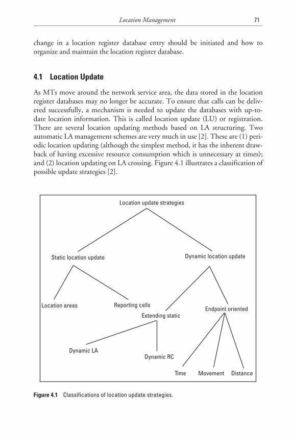
change in a location register database entry should be initiated and how toorganize and maintain the location register database.

4.1 Location Update

As MTs move around the network service area, the data stored in the locationregister databases may no longer be accurate. To ensure that calls can be deliv-ered successfully, a mechanism is needed to update the databases with up-to-date location information. This is called location update (LU) or registration.There are several location updating methods based on LA structuring. Twoautomatic LA management schemes are very much in use [2]. These are (1) peri-odic location updating (although the simplest method, it has the inherent draw-back of having excessive resource consumption which is unnecessary at times);and (2) location updating on LA crossing. Figure 4.1 illustrates a classification ofpossible update strategies [2].

Location Management 71

Location update strategies

Static location update Dynamic location update

Location areas Reporting cells

Extending staticEndpoint oriented

Dynamic LADynamic RC

Time Movement Distance

Figure 4.1 Classifications of location update strategies.

4.1.1 Location Update Static Strategies

In a static update strategy, there is a predetermined set of cells at which locationupdates may be generated. Whatever the nature of mobility of an endpoint,location updates may only be generated when, but not necessarily every time,the endpoint enters one of these cells. Two approaches to static updating are asfollows:

1. LAs (also referred to as paging or registration areas) [3]: In this approach,the service area is partitioned into groups of cells with each group as anLA. An endpoint’s position is updated if and only if the endpointchanges LAs. When an endpoint needs to be located, paging is doneover the most recent LA visited by the endpoint. Location tracking inmany second-generation cellular systems, including GSM [4] andIS-41 [5], is based on LAs [6]. Several strategies for LA planning in acity environment are evaluated in [7]. These include strategies thattake into account geographical criteria (such as population distributionand highway topology) and user mobility characteristics.

2. Reporting cells (or reporting centers) [8]: In this approach, reportingcells, a subset of the cells, are designated as the only ones from whichan endpoint’s location may be updated. When an endpoint needs to belocated, a search is conducted in the vicinity of the reporting cell fromwhich the most recent update was generated. In [8], the problem ofwhich cells should be designated as reporting cells in order to optimizea cost function is addressed for various cell topologies.

The principal drawback to static update strategies is that they do not accu-rately account for user mobility and frequency of incoming calls. For example,even though a mobile endpoint may remain within a small area, it may causefrequent location updates if that area happens to contain a reporting cell.

4.1.2 Location Update Dynamic Strategies

In a dynamic update strategy, an endpoint determines when an update shouldbe generated, based on its movement. Thus, an update may be generated in anycell. A natural approach to dynamic strategies is to extend the static strategies toincorporate call and mobility patterns. The dynamic LA strategy proposed in [9]dynamically determines the size of an endpoint’s LA according to the endpoint’sincoming call arrival rate and mobility. Analytical results presented in [9] indi-cate that this strategy is an improvement over static strategies when call arrivalrates are user-dependent or time-dependent. The dynamic reporting centersstrategy proposed in [10] uses easily obtainable information to customize thechoice of the next set of reporting cells at the time of each location update. In


TEAMFLY

Team-Fly®

particular, the strategy uses information recorded at the time of the endpoint’slast location update, including the direction of motion, to construct an asym-metric distance-based cell boundary and to optimize the cell search order. In[11], three dynamic strategies are described in which an endpoint generates alocation update (1) every T seconds (time-based), (2) after every M cell crossings(movement-based), or (3) whenever the distance covered (in terms of number ofcells) exceeds D (distance-based). Distance-based strategies are inherently themost difficult to implement since the mobile endpoints need information aboutthe topology of the cellular network. It was shown in [11], however, that formemoryless movement patterns on a ring topology, distance-based updatingoutperforms both time-based and movement-based updating. In [1], a set ofdynamic programming equations is derived and used to determine an optimalupdating policy for each endpoint, and this optimal policy is in fact distance-based. Strategies that minimize location-tracking costs under specified delayconstraints (i.e., the time required to locate an endpoint) have also been pro-posed. In [12], a paging procedure is described that minimizes the meannumber of locations polled with a constraint on polling delay, given a probabil-ity distribution for endpoint locations. A distance-based update scheme and acomplementary paging scheme that guarantee a predefined maximum delay onlocating an endpoint are described in [13]. This scheme uses an iterative algo-rithm to determine the optimal update distance D that results in minimum costwithin the delay bound.

In organizing the location database, one seeks to minimize both thelatency and the overhead, in terms of the amount of storage and the number ofmessages required, in accessing location information. These are, in general,counteracting optimization criteria. Most solutions to the location databaseorganization problem select a point, which is a three-way trade-off betweenoverhead, latency, and simplicity. The simplest approach to location databaseorganization is to store all endpoint identifier-to-address mappings in a singlecentral place. For large numbers of reasonably mobile endpoints, however, thisapproach becomes infeasible in terms of database access time and storage spaceand also represents a single point of failure.

The next logical step in location database organization is to partition thenetwork into a number of smaller pieces and place a portion of the locationdatabase in each piece. Such a distributed approach is well suited to systemswhere each subscriber is registered in a particular area or home. With thisorganization, the location database in an area contains the locations of all end-points that have that area for a home. When the endpoint moves out of its homearea, it updates its home location database to reflect the new location. The HLRand VLR schemes of emerging wireless cellular networks [6] are an example ofthis approach, as are the Mobile IP scheme [14] for the Internet and the GSM-based General Packet Radio Switching (GPRS) Network for data transport over


cellular networks. Studies [15, 16] have shown that with predicted levels ofmobile users, signaling traffic may exceed acceptable levels. Thus, researchershave considered augmenting this basic scheme to increase its efficiency undercertain circumstances. For instance, in [17], per-user caching is used to reuselocation information about a called user for subsequent calls to that user, and isparticularly beneficial for users with high call-to-mobility ratios (i.e., the fre-quency of incoming calls is much larger than the frequency of location updates).In [18], “local anchoring” is used to reduce the message overhead by reportinglocation changes to a nearby VLR instead of to the HLR, thus increasing thelocation-tracking efficiency when the call-to-mobility ratio is low and theupdate cost is high. As with most large organizational problems, a hierarchicalapproach provides the most general and scalable solution. By hierarchicallyorganizing the location database, one can exploit the fact that many movementsare local. Specifically, by confining LU propagation to the lowest level (in thehierarchy) containing the moving endpoint, costs can be made proportional tothe distance moved. Several works address this basic theme. In [19], a hierarchyof regional directories is prescribed where each regional directory is based on adecomposition of the network into regions. Here, the purpose of the ith-levelregional directory is to enable tracking of any user residing within a distance of2i. This strategy guarantees overheads that are polylogarithmic in the size anddiameter of the network. In [20], the location database is organized so as tominimize the total rate of accesses and updates. This approach takes intoaccount estimates of mobility and calling rates between cells and a budget onaccess and update rates at each database site. In [21], location database organiza-tion takes into account the user profile of an endpoint (i.e., the predefined pat-tern of movement for the endpoint). Partitions of the location database areobtained by grouping the locations among which the endpoint moves fre-quently and by separating those to which the endpoint relocates infrequently.Each partition is further partitioned in a recursive fashion, along the same lines,to obtain a location database hierarchy.

In the above strategies, the emphasis is on reducing update overhead, butit is equally important to reduce database access latency. One strategy for doingso is replication, where identical copies of the database are kept in various partsof the network so that an endpoint location may be obtained using a low-latencyquery to a nearby server. The problem here is to decide where to store the repli-cations. This is similar to the classical database allocation [22] and file allocation[23] problems, in which databases or files are replicated at sites based on query-update or read-write access patterns. In [24], the best zones for replication arechosen per endpoint location entry, using a minimum-cost maximum-flowalgorithm to decide where to replicate the database, based on the calling andmobility patterns for that endpoint.


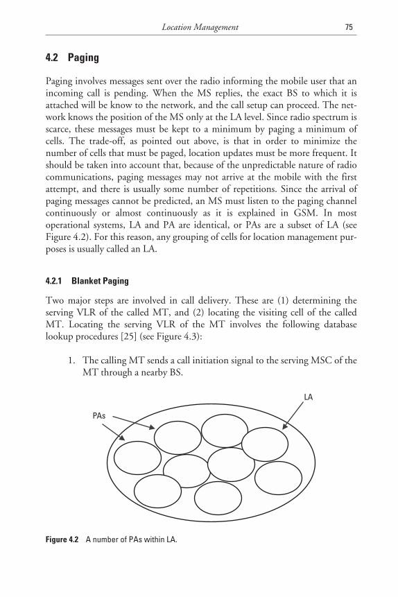
4.2 Paging

Paging involves messages sent over the radio informing the mobile user that anincoming call is pending. When the MS replies, the exact BS to which it isattached will be know to the network, and the call setup can proceed. The net-work knows the position of the MS only at the LA level. Since radio spectrum isscarce, these messages must be kept to a minimum by paging a minimum ofcells. The trade-off, as pointed out above, is that in order to minimize thenumber of cells that must be paged, location updates must be more frequent. Itshould be taken into account that, because of the unpredictable nature of radiocommunications, paging messages may not arrive at the mobile with the firstattempt, and there is usually some number of repetitions. Since the arrival ofpaging messages cannot be predicted, an MS must listen to the paging channelcontinuously or almost continuously as it is explained in GSM. In mostoperational systems, LA and PA are identical, or PAs are a subset of LA (seeFigure 4.2). For this reason, any grouping of cells for location management pur-poses is usually called an LA.

4.2.1 Blanket Paging

Two major steps are involved in call delivery. These are (1) determining theserving VLR of the called MT, and (2) locating the visiting cell of the calledMT. Locating the serving VLR of the MT involves the following databaselookup procedures [25] (see Figure 4.3):

1. The calling MT sends a call initiation signal to the serving MSC of theMT through a nearby BS.


LA

PAs

Figure 4.2 A number of PAs within LA.

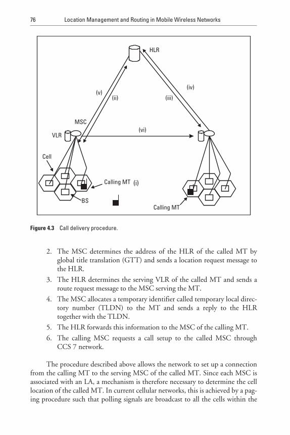
2. The MSC determines the address of the HLR of the called MT byglobal title translation (GTT) and sends a location request message tothe HLR.

3. The HLR determines the serving VLR of the called MT and sends aroute request message to the MSC serving the MT.

4. The MSC allocates a temporary identifier called temporary local direc-tory number (TLDN) to the MT and sends a reply to the HLRtogether with the TLDN.

5. The HLR forwards this information to the MSC of the calling MT.

6. The calling MSC requests a call setup to the called MSC throughCCS 7 network.

The procedure described above allows the network to set up a connectionfrom the calling MT to the serving MSC of the called MT. Since each MSC isassociated with an LA, a mechanism is therefore necessary to determine the celllocation of the called MT. In current cellular networks, this is achieved by a pag-ing procedure such that polling signals are broadcast to all the cells within the


(vi)

(v)(ii) (iii)

VLR

MSC

HLR

Calling MT

Calling MTBS

Cell

(iv)

(i)

Figure 4.3 Call delivery procedure.

residing LA of the called MT over a forward control channel. On receiving thepolling signal, the MT sends a reply over a backward control channel, whichallows the MSC to determine its current residing cell. This is called blanket-paging method. In a selective paging scheme, instead of polling all the cells in anLA, a few cells are polled at a time. The cluster of cells polled at a time consti-tutes the PA. Here, a factor called the granularity factor, K is defined as the ratioof the number of cells in the PA to the number of cells in the LA. K denotes thefineness in the polling scheme. In a purely sequential polling scheme, K = 1/Sj

where the granularity factor is one in the case of blanket polling, and Sj is thenumber of cells in the jth LA.

4.2.2 Different Paging Procedures

Rose [26] developed methods for balancing call registration and paging. Theprobability distribution on the user location as a function of time is eitherknown or can be calculated, the lower bounds on the average cost of paging areused in conjunction with a Poisson incoming-call arrival model to formulate thepaging and registration optimization problem in terms of timeout parameters.

In their other work [12], efficient paging procedures are used to minimizethe amount of bandwidth expended in locating a mobile unit. Given the prob-ability distribution on user location, they have shown that the optimal pagingstrategy, which minimizes the expected number of locations polled, is to queryeach location sequentially in order of decreasing probability. Since a sequentialsearch over many locations may impose unacceptable polling delay, they consid-ered optimal paging subject to delay constraint.

In [13], they have proposed a mobile user location mechanism that incor-porates a distance-based LU scheme and a paging mechanism that satisfied pre-defined delay requirements. In [27], they have introduced a mobility trackingmechanism that combines a movement-based LU policy with a selective pagingscheme. This selective paging scheme decreases the location tracking cost undera small increase in the allowable paging delay.

In [28], they explored tracking strategies for MUs in personal communica-tion networks, which are based on the topology of cells. The notion oftopology-based strategies was introduced in a general form in this work. In par-ticular, the known PAs, overlapping PAs, reporting centers and distance-basedstrategies were covered by this notion.

This work [29] proposed a method, which aims at the reduction of signal-ing overhead on the radio link, produced by the paging procedure. The key ideais the application of a multiple step paging strategy, which operates as follows:At the instance of a call terminating to an MU which roams within a certain LA,paging is initially performed in a portion of the LA (the PA) that the so-called“paging related information” indicates. Upon no paging response, the MU is


paged in the complementary portion of the LA—this phase can be completed inmore than one (paging) step. Several “intelligent” paging strategies were definedin this work. In [30], various paging schemes were presented for locating MUsin wireless networks. Paging costs and delay bounds are considered since pagingcosts are associated with bandwidth utilization and delay bounds influence callsetup time. To reduce the paging costs, three paging schemes, reverse, semire-verse, and uniform, were introduced to provide a simple way of partitioning theservice areas and decrease the paging costs based on each MT’s location prob-ability distribution.

The several paging strategies mainly based on blanket paging were appliedto reduce the paging costs as well as update costs associated with constraints.These strategies discussed briefly above were widely used and few of them areapplied in industry. In spite of having widespread use of those paging strategies,some disadvantages have been found. In the next section, a few new pagingschemes are discussed to overcome the disadvantages in the different blanketpaging schemes.

4.3 Intelligent Paging Scheme

The movement of MTs is modeled according to some ergodic, stochasticprocess [31]. To provide ubiquitous communication link, irrespective of thelocation of MTs, the BSs provide a continuous coverage during the call and inthe idle state also. When an incoming call comes to an MT, which roams withina certain LA, paging is initially performed within a portion of the LA, which is asubset of the actual LA. This portion of the LA, which is a set of base stations ofpaging (BSPs), is termed a PA. Intelligent paging is a multistep paging strategy[7], which aims at determining the proper PA within which the called MT cur-rently roams. In order to quantitatively evaluate the average cost of paging,time-varying probability distributions on MTs are required. These distributionsmay be derived from the specific motion models, approximated via empiricaldata, or even provided by the MTs in the form of a partial itinerary at the timeof the last contact. It is assumed that

1. The probability density function of the speed of MTs is known.

2. The process of movement of MTs is isotropic, Brownian motion [32]with drift. In the one-dimensional version of Brownian motion, anMT moves by one step ∆x to the right with some probability, p and tothe left with probability q, and stays there with probability (1 – p – q)for each time step ∆t . Given that the MT starts at time t = 0 for posi-tion x = 0, the Gaussian PDF on the location of an MT is given by:


P x t Dt ex tk x vt x vt Dt

( ). ( )*( )/( ( )) ( )= − − − −π 0 5 (4.1)

where v = (p – q)×(∆x/∆t ) is the drift velocity and D = 2((1 – p) p +(1 – q) q + 2pq) (∆x)2/ ∆t is the diffusion constant, both functions ofthe relative values of time and space steps. Drift is defined as mean ve-locity in a given direction and is used to model directed traffic such asvehicles along a highway;

3. Time elapsed since the last known location;

4. The paging process described here is rapid enough for the rate ofmotion of the MT (i.e., the MT to be found does not change its loca-tion during the paging process).

The algorithm of an intelligent paging process on arrival of a pagingrequest (PR) is given below:

While PR is attached while MT is not busy

if current traffic load exceeds threshold trafficload

initialize the incremental counter i = 0;select the proper PA;page within the selected PA;if reply against PR received

then stop;else

while (imaximum value of incremental counter i)do

page within another PA;increase the incremental counter i = i + 1;

elseapply blanket paging;

The intelligent paging strategy maps the cells inside the LA comprising Scells into a probability line at the time of arrival of the incoming call. This map-ping depends on factors such as the mobility of the MT, its speed profile, theincoming call statistics, and the state of the MT at that instant. This procedureis called attachment. If it is detached, the PR is cancelled. If it is busy, a relationbetween the MT and the network already exists, and therefore paging is notrequired. If it is free, the network proceeds for paging upon receipt of a PR (seeabove algorithm). In the intelligent paging scheme, the network determines the


probability of occupancy of the called MT in different cells in an LA. Theseprobabilities are arranged in descending order. The order in which cells are to bepolled depends on the ordered set of probability occupancy vector. In each pag-ing cycle, the MSC serves PRs stored in its buffer, independently of each other.It is done by assigning a BS to each of the n requests in the buffer according toan assignment policy. The jth PR may be sent to the ith BS, in order to be pagedin the corresponding cell. There are many ways to generate such assignments.Two methods will be presented subsequently in this chapter as part of the pro-posed intelligent paging scheme. If the buffer size is n and there are k PAs(denoted by A1, A2,..., Ak), then we can write:

A A A Sk1 2∪ ∪ =.....

Ai Aj∪ =φ

This means that the PAs are mutually exclusive and collectively exhaustive.Paging and channel allocation packets from a BS to MTs are multiplexed streamin a forward signaling channel. Paging rate represents the average number ofpaging packets, which arrives at a BS during unit time. Paging signals are sent tothe BSs via landlines and are broadcast over the forward signaling channel. Aseach attached MT in the LA constantly monitors the paging channels to checkwhether it is paged or not, the distributor in the MSC which is a part of Mobil-ity Manager (MM) allocates the distribution of PRs to the BSs for each pagingcycle based on the information collected over the previous paging cycle. As soonas an MT is found, the corresponding PR is purged from the buffer and a newPR replaces it. The function of the distributor in the MM is to map the PRs tothe PAs:

g : (PR1, PR2,..., PRn)→ (A1, A2,..., Ak)

Depending on the nature of polling, there may be two types of search.These are sequential and parallel-o-sequential. In purely sequential polling, onecell is polled in a paging cycle. Sometimes, due to delay constraint, instead ofpolling one cell at a time, we poll a cluster of cells in an LA. This is calledparallel-o-sequential intelligent paging (PSIP) which is a special case of sequen-tial intelligent polling (SIP).

The network first examines whether a multiple-step paging strategy shouldbe applied or not. The decision is based on the current traffic load. Normally,when this load exceeds a threshold value, a multiple-step paging strategy isemployed. In the very first phase, the network decides whether checking the cur-rent status of the MT needs paging. The network then examines whether the


appropriate type of paging is blanket paging or multiple-step paging. Thegranularity factor K shows fineness in polling. In general, the granularity factoris defined as

K = (number of cells to be polled in a cycle)/(number of cells in an LA)

The maximum value of the granularity factor is 1, when all cells in an LAare polled in one polling cycle. The granularity factor in SIP is, K SIP =1/(number of cells in an LA). The granularity factor in PSIP is K PSIP = (numberof cells in the cluster)/(number of cells in an LA).

We assumed a perfect paging mechanism where an MT will alwaysrespond to a paging signal meant for it, provided it receives the PR. However,situations may arise that leave an MT undetected even though the distributor inthe MSC is able to select the corresponding BS and initiate a PR for it. Such asituation will arise when there are more PRs assigned to a BS by the distributorthan the number of paging channels available in a cycle. As there are only l pag-ing channels per BS, the PRs in excess of l will be considered to be blocked.These excess PRs will be attempted for sending to select BSs in subsequent pag-ing cycles. So the called MT may be inside the area of an overloaded cell. But thePR for it might be blocked in a paging cycle. So, the distributor must keep trackof the number of times a search has been attempted for the PR.

The application of intelligent paging includes the event of paging failuresdue to wrong predictions of the locations of the called MT. In such cases,another step, or more than one step, will be required (i.e., the called MT will bepaged in other PAs). Continuous unsuccessful paging attempts may lead tounacceptable network performance in terms of paging delay. Moreover, the pag-ing cost will also increase with each unsuccessful attempt to locate the calledMT. In such cases, the network does not preclude the option of single-step pag-ing at a certain intermediate point of search.

4.3.1 Sequential Intelligent Paging

In sequential intelligent paging schemes, one cell is polled at a time and theprocess continues until such time the called MT is found or timeout occurswhichever is earlier. The selection of the cell to be polled sequentially dependson the value of the occupancy probability vector, which is based on the stochas-tic modeling delineating the movement of the MT. In SIP, the PRs are stored ina buffer of the MSC and each PR is sent to that BS where there is maximumprobability of finding the called MT. When the paging is unsuccessful during apolling cycle the MT is sequentially paged in other cells of the LA that have notbeen polled so far. This phase is completed in one, or more than one, pagingstep(s). The sequential paging algorithm is given below:


STEP 1: When an incoming call arrives, calculate theoccupancy probability vector, [P] of an MT forthe cells in the LA based on the probabilitydensity function, which characterizes themotion of the MT;

STEP 2: Sort the elements of [P] in descending order;STEP 3.0: FLAG = False;

i = 1;STEP. 3.1: Poll the ith cell for i(S;STEP. 3.2: If the MT is found

FLAG = True;Go to ENDSTEP;

STEP. 4.0:If timeout occurs

Go to ENDSTEP;Else

i = i + 1;Go to STEP 3.1;

EndifENDSTEP: If FLAG = True

"Declare Polling is Successful";Else"Declare Polling is Unsuccessful";Endif

As extra processing is required at the MSC, an inherent delay will be asso-ciated with this process (i.e., before the PR is sent to the appropriate BS). Thisdelay includes the determination of the probabilities in different cells, sorting ofthese probabilities in descending order and polling the cells sequentially depend-ing on those values. This delay will be added to the call setup process. Theamount of this delay will be ~ (O (S ) + O (S log S ) + O (S/2)).

4.3.2 PSIP

PSIP is a special case of SIP where K 1. Instead of polling a single cell in eachcycle, here we partition the LAs into several PAs and poll those PAs sequentiallycomprising more than one cell. The benefit that accrues out of PSIP is a signifi-cant improvement in the expected discovery rate of called MTs and the over-whelming reduction in paging cost and signaling load. The number of steps inwhich the paging process should be completed depends on the allowed delayduring paging. The application of PSIP also includes the event of paging failuresdue to unsuccessful predictions of the location of called MT. In such cases, mul-tiple steps are required and the called MT is paged in another portion of the LA.To obviate the deterioration of the network performance in such a situation andminimize the number of paging steps, the network should guarantee the forma-tion of PAs such that the PSFP is high (typical value >90%). So, the PA shouldconsist of those cells where the sum of probabilities of finding the called MT isgreater than or equal to the typical value chosen for PSFP. The parallel-o-sequential paging algorithm is given below:


TEAMFLY

Team-Fly®

STEP 1: When an incoming call arrives, find out the current state of the called MT;

STEP 2: If MT is detachedPR is cancelled;Go to ENDSTEP;

ElseIf MT is busy (location is known)

go to ENDSTEP;Else

Find granularity factor K;Endif

STEP 3: If granularity factor is 1Poll all the cells;go to ENDSTEP;

Elsefind out [P] , the occupancy probability vectorof the MT for the cells in the LA, based on theprobability density function which characterizesthe motion of the MT;

EndifSTEP 4: Sort the elements of [P] in descending order;

Set all the cells as unmarked ;STEP 5.0: Select a proper PA consisting of "unmarked"

cells for which Σpi>PSFP;FLAG = False;

STEP 5.1: Poll ith cluster and label the cells in ithcluster as marked

STEP 5.2: if the MT is foundFLAG = True;Go to ENDSTEP;

STEP 6.0:If timeout occursGo to ENDSTEP;

ElseGo to STEP 5.0;

EndifENDSTEP: If FLAG = True

Declare: "Polling is Successful" ;Else

Declare: "Polling is Unsuccessful" ;Endif

4.3.3 Comparison of Paging Costs

In the conventional or the blanket paging, upon arrival of an incoming call, thepaging message is broadcast from all the BSs in the LA. That means all the cellsin the LA are polled at a time for locating the called MT (i.e., each MT is pagedS times before the called MT is discovered). The polling cost per cycle is

C SAp p pconv

cell= ρµΤ Β (4.2)

The SIP strategy, described here, aims at the significant reduction in loadof paging signaling on the radio link by paging a cell sequentially. PRs arrive


according to a Poisson process at the buffer of the MSC. The distributor issuesthe PRs to appropriate BSs. These PRs are queued at the location and servicedon an FCFS basis at the average rate ζ . The result may be a success or a failure.The results of completed polls are fed back to the controller in the BS for furtherappropriate action. As pointed out earlier, a called MT may not be found duringa paging cycle. Either the number of paging channels may be insufficient toaccommodate the PR in a particular cycle, or the search for the called MT in thecell results in a failure. In both cases, the polling process goes through more thanone cycle. So, the paging cost per polling cycle in this scheme is

C K SA z T Bp p pSIP SIP

cell= +ρµ( )1 (4.3)

The variable z accounts for the unsuccessful PRs from the previous cycledue to either of the two reasons, so z depends on the success rate, timeout dura-tion, and the number of paging channels available per BS. In GSM, assumingthat a sufficient channel for paging is there, z becomes zero. In the best case (i.e.,when the called MT is found during the first polling cycle of SIP), z is also zero.In the worst case, all the cells in the LA are to be polled before the MT is found.Then the polling cost just exceeds that in GSM. Moreover, the delay is also at amaximum (i.e., S units). There may be a situation when the polling cost in a SIPscheme exceeds the cost in blanket polling significantly. If the MT resides in acell with a low probability of occupancy and returns to one of the cells that ispolled already after the polling cycle, the called MT will not be found even afterpolling all the cells in the LA. Such an incidence is likely when the number ofcells is greater, a few cells have the same probability of occupancy, and the MT isvery mobile. In this case, the call is blocked or the cells are polled sequentiallyonce again to find the MT. So, K has an inverse effect on z. The granularity fac-tor K is generally chosen to be more than one to avoid such a scenario. The pag-ing cost per polling cycle in PSIP is

C K SA z T Bp p pSIP SIP

cell= +ρµ( )1 (4.4)

The variable z also accounts for the unsuccessful PRs from the previouscycle. As mentioned earlier also, K is chosen such that PSFP > 0.9. The optimumvalue of K varies from case to case.

4.4 More Paging Schemes

Assume that each LA consists of the same number N of cells in the system [30].The worst-case paging delay is considered as delay bound D in terms of the


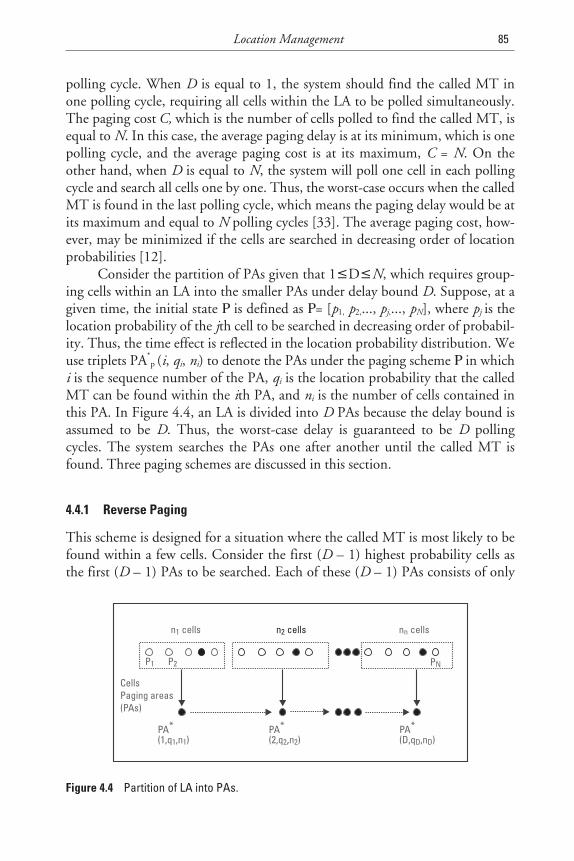
polling cycle. When D is equal to 1, the system should find the called MT inone polling cycle, requiring all cells within the LA to be polled simultaneously.The paging cost C, which is the number of cells polled to find the called MT, isequal to N. In this case, the average paging delay is at its minimum, which is onepolling cycle, and the average paging cost is at its maximum, C = N. On theother hand, when D is equal to N, the system will poll one cell in each pollingcycle and search all cells one by one. Thus, the worst-case occurs when the calledMT is found in the last polling cycle, which means the paging delay would be atits maximum and equal to N polling cycles [33]. The average paging cost, how-ever, may be minimized if the cells are searched in decreasing order of locationprobabilities [12].

Consider the partition of PAs given that 1≤D≤N, which requires group-ing cells within an LA into the smaller PAs under delay bound D. Suppose, at agiven time, the initial state Ρ is defined as Ρ= [p1, p2,..., pj,..., pN], where pj is thelocation probability of the jth cell to be searched in decreasing order of probabil-ity. Thus, the time effect is reflected in the location probability distribution. Weuse triplets PA*

p (i, qi, ni) to denote the PAs under the paging scheme Ρ in whichi is the sequence number of the PA, qi is the location probability that the calledMT can be found within the ith PA, and ni is the number of cells contained inthis PA. In Figure 4.4, an LA is divided into D PAs because the delay bound isassumed to be D. Thus, the worst-case delay is guaranteed to be D pollingcycles. The system searches the PAs one after another until the called MT isfound. Three paging schemes are discussed in this section.

4.4.1 Reverse Paging

This scheme is designed for a situation where the called MT is most likely to befound within a few cells. Consider the first (D – 1) highest probability cells asthe first (D – 1) PAs to be searched. Each of these (D – 1) PAs consists of only


P1 P2

n cells1 n cells2

PN

n cellsn

PA*(1,q ,n )1 1

PA*(2,q n )2 2,

PA*(D,q ,n )D D

CellsPaging areas(PAs)

Figure 4.4 Partition of LA into PAs.

one cell. Then the remaining (N – D + 1) lower probability cells are lumpedtogether to be the last PA, (i.e., the Dth PA). The newly formed PAs becomePA*

r (1, p1, 1), PA*r (2, p2, 1),..., PA*

r (D – 1, pD – 1, 1), PA*r (D, qD, N – D + 1),

where r denotes the reverse paging scheme.

4.4.2 Semireverse Paging

Since the average paging cost can be minimized by searching cells in decreasingorder of location probability, if a delay bound D is not applied [12], intuitively,the paging cost can be reduced by searching the PAs in decreasing order of prob-ability. Under semireverse paging schemes, a set of PAs is created in a nonin-creasing order of location probabilities. First, combine the two cells with thelowest location probabilities into one PA, and then reorder all PAs in nonin-creasing order of location probabilities. Keep combining the two PAs with thelowest probabilities and reorder them until the total number of PAs is equal toD. If two PAs have the same probability, the PA with fewer cells has higher pri-ority, (i.e., its sequence number is smaller). Semireverse paging schemes guaran-tee that the location probability of each PA is in a nonincreasing order.However, the cell with lower probability may be searched before the cell withhigher probability because the initial sequence of the cells is reordered duringthe semireverse paging procedure.

4.4.3 Uniform Paging

Under a uniform paging scheme, the LA is partitioned into a series of PAs insuch a way that all PAs consist of approximately the same number of cells. Theuniform paging procedure is as follows:

• Calculate the number of cells in each PA as n N D0 = where N =n0D + k.

• Determine a series of PAs as PA*u (1, p1, 1), PA*u (2, p2, 1),..., PA*

u (D,qD, nD). Note that there are n0 cells in each of the first (D – k) PAs andthere are n0 + 1 cells in each of the remaining PAs. This means n1 = n2

=... = nD – k = n0, and nD – k + 1 =... = nD = n0 + 1. For example, the first PAconsists of n0 cells and the last PA, (i.e., Dth PA), consists of n0 + 1 cells.

• The network polls one PA after another sequentially until the calledMT is found.


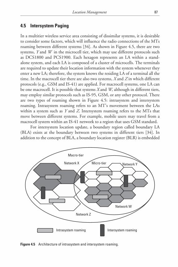
4.5 Intersystem Paging

In a multitier wireless service area consisting of dissimilar systems, it is desirableto consider some factors, which will influence the radio connections of the MTsroaming between different systems [34]. As shown in Figure 4.5, there are twosystems, Y and W in the microcell tier, which may use different protocols suchas DCS1800 and PCS1900. Each hexagon represents an LA within a stand-alone system, and each LA is composed of a cluster of microcells. The terminalsare required to update their location information with the system whenever theyenter a new LA; therefore, the system knows the residing LA of a terminal all thetime. In the macrocell tier there are also two systems, X and Z in which differentprotocols (e.g., GSM and IS-41) are applied. For macrocell systems, one LA canbe one macrocell. It is possible that systems X and W, although in different tiers,may employ similar protocols such as IS-95, GSM, or any other protocol. Thereare two types of roaming shown in Figure 4.5: intrasystem and intersystemroaming. Intrasystem roaming refers to an MT’s movement between the LAswithin a system such as Y and Z. Intersystem roaming refers to the MTs thatmove between different systems. For example, mobile users may travel from amacrocell system within an IS-41 network to a region that uses GSM standard.

For intersystem location update, a boundary region called boundary LA(BLA) exists at the boundary between two systems in different tiers [34]. Inaddition to the concept of BLA, a boundary location register (BLR) is embedded


Intersystem roamingIntrasystem roaming

Macro tier-

Micro-tierNetwork X

Network Z

Network W

Network Y

Figure 4.5 Architecture of intrasystem and intersystem roaming.

in the boundry interworking unit (BIU). A BLR is a database cache to maintainthe roaming information of MTs moving between different systems. The roam-ing information is captured when the MT requests a location registration in theBLA. The BLRs enable the intersystem paging to be implemented within theappropriate system that an MT is currently residing in, thus reducing the pagingcosts. Therefore, the BLR and the BIU are accessible to the two adjacent systemsand are collocated to handle the intersystem roaming of MTs. The VLR and theMSC, however, provide roaming information within a system and deal with theintrasystem roaming of MTs. Besides, there is only one BLR and one BIUbetween a pair of neighboring systems, but there may be many VLRs and MSCswithin a stand-alone system.

When a call connection request arrives at X, the call will be routed to thelast registered LA of the called MT. Given that the last registered LA within X isadjacent to Y, the system needs to perform the following steps to locate the MT:

1. Sends a query signal to the BLR between X and Y to obtain the MT’slocation information. This step is used to ascertain whether the MThas crossed the boundary or not.

2. If the MT has already moved to Y, searches only the LA in Y. Other-wise, the last registered LA within X will be searched. Within networkX or Y, one or multiple polling messages are sent to the cells in the LAaccording to a specific paging scheme.

As a result, only one system (X or Y ) is searched in the paging process forintersystem roaming terminals. This approach will significantly reduce the sig-naling cost caused by intersystem paging. In particular, it is very suitable for thehigh traffic environment because it omits the searching of two adjacent systems.Moreover, since the BLR is an additional level of cache database, it will notaffect the original database architecture. Another advantage of the BLR is that itreduces the zigzag effect caused by intersystem roaming. For example, when anMT is moving back and forth on the boundary, it only needs to update theinformation in the BLR instead of contacting the HLRs. If the new BLR con-cept is not used, the intersystem paging can still take place. The system willsearch X first, if the called MT cannot be found, then Y will be searched. Thismethod increases the paging cost as well as the paging delay, thus degrading thesystem performance.

4.6 IP Micromobility and Paging

Recent research [35] in Mobile IP has proposed that IP should take supportfrom the underlying wireless network architecture to achieve good performancefor handover and paging protocols. Recent IETF work defines requirements for


layer 2 (the data link layer of the OSI model) to support optimized layer 3 (thenetwork layer of the OSI model) handover and paging protocols. Layer 2 cansend notification to layer 3 that a certain event has happened or is about to hap-pen. The notification is sent using a trigger. IP micromobility and paging proto-cols require support from underlying wireless infrastructure.

Layer 2 can help layer 3 by providing information in the form of triggers.A trigger can be defined as an abstraction of notification from layer 2 that a cer-tain event has happened or is about to happen. In [36], various ways of imple-menting triggers are discussed. A trigger may be implemented using system calls.The operating system may allow an application thread to register callback for alayer 2 trigger, using system calls of an application-programming interface(API). A system call returns when that particular event is fired in layer 2. Eachtrigger is defined by three parameters:

1. The event that causes trigger to fire;

2. The entity that receives the trigger;

3. The parameters delivered with the trigger.

Triggers were defined to aid low-latency handover in Mobile IP [37].Another set of triggers was defined in [38] to aid IP paging protocols. CDMA,for example, works in conjunction with Mobile IP to support mobility in IPhosts. IP paging is a protocol used to determine the location of a dormant (amode that conserves battery by not performing frequent updates) Mobile Node(MN). Paging triggers were defined in [38] to aid movement of a MN in multi-ple IP subnets in the same layer 2 PA. Paging triggers aid the MN in enteringdormant mode in a graceful manner and make the best use of paging providedby underlying wireless architecture.

4.7 Location Management

Location management schemes are essentially based on users’ mobility andincoming call rate characteristics. It is two-stage process that enables the net-work to discover the current attachment point of the MU for call delivery. Thefirst stage is location registration or location update. In this stage, the MT peri-odically notifies the network of it new access point, allowing the network toauthenticate the user and revise the user’s location profile. The second stage iscall delivery. Here, the network is queried for the user location profile and thecurrent position of the mobile host is found. Current techniques for locationmanagement involve database architecture design and the transmission of sig-naling messages between various components of a signaling network. Other


issues include: security, dynamic database updates, querying delays, terminalpaging methods, and paging delays.

There are two standards for location management currently available:Electronics and Telecommunications Industry Associations (EIA/TIA) IS-41[39] and the GSM mobile application part (MAP) [6]. The IS-41 scheme iscommonly used in North America for AMPS, IS-54, IS-136, and PACS net-works, while the GSM MAP is mostly used in Europe for GSM and DCS1800networks. Both standards are based on a two-level data hierarchy. Location reg-istration procedures update the location databases (HLR and VLRs) andauthenticate the MT when up-to-date location information of an MT is avail-able. Call delivery procedures locate the MT based on the information availableat the HLR and VLRs when a call for an MT is initiated. The IS-41 and GSMMAP location management strategies are very similar. While GSM MAP isdesigned to facilitate personal mobility and to enable user selection of networkprovider, there are a lot of commonalities between the two standards [4, 25].The location management scheme may be categorized in several ways.

4.7.1 Without Location Management

In this level 0 method, no location management is realized [40]; the system doesnot track the mobiles. A search for a called user must therefore be done over thecomplete radio coverage area and within a limited time. This method is usuallyreferred to as the flooding algorithm [41]. It is used in paging systems because ofthe lack of an uplink channel allowing a mobile to inform the network of itswhereabouts. It is also used in small private mobile networks because of theirsmall coverage areas and user populations. The main advantage of not locatingthe MTs is obviously simplicity; in particular, there is no need to implementspecial databases. Unfortunately, it does not fit large networks dealing with highnumbers of users and high incoming call rates.

4.7.2 Manual Registration in Location Management

This level 1 method [40] is relatively simple to manage because it only requiresthe management of an indicator, which stores the current location of the user.The mobile is also relatively simple; its task is just limited to scanning the chan-nels to detect paging messages. This method is currently used in telepoint cord-less systems (such as CT2). The user has to register each time he or she moves toa new island of CT2 beacons. To page a user, the network first transmits mes-sages through the beacon with which he or she registered and, if the mobile doesnot answer, extends the paging to neighboring beacons. The main drawback ofthis method is the constraint for a user to register each time he or she moves.


4.7.3 Automatic Location Management Using LA

Presently, this level 2 location method [40] most widely implemented in first-and second-generation cellular systems (e.g., NMT, GSM, IS-95) makes use ofLAs (see Figure 4.1). In these wide-area radio networks, location management isdone automatically. LAs allow the system to track the mobiles during theirroaming in the network(s): subscriber location is known if the system knows theLA in which the subscriber is located. When the system must establish a com-munication with the mobile (to route an incoming call, typically), the pagingonly occurs in the current user LA. Thus, resource consumption is limited tothis LA; paging messages are only transmitted in the cells of this particular LA.Implementing LA-based methods requires the use of databases. Generally, ahome database and several visitor databases are included in the networkarchitecture.

4.7.4 Memoryless-Based Location Management Methods

All methods included are based on algorithms and network architecture, mainlyon the processing capabilities of the system.

4.7.4.1 Database Architecture

LA partitioning, and thus mobility management cost, partly relies on the systemarchitecture (e.g., database locations). Thus, designing an appropriate databaseorganization can reduce signaling traffic. The various database architectures areproposed with this aim [25, 42–44]. An architecture where a unique centralizeddatabase is used is well-suited to small and medium networks, typically based ona star topology. The second one is a distributed database architecture, whichuses several independent databases according to geographical proximity or serv-ice providers. It is best-suited to large networks including subnetworks managedby different operators and service providers. The GSM worldwide network,defined as the network made up of all interconnected GSM networks in theworld, can be such an example of a large network. The third case is the hybriddatabase architecture that combines the centralized and distributed databasearchitectures. In this case, a central database (HLR-like) is used to store all userinformation. Other smaller databases (VLR-like) are distributed all over the net-work. These VLR databases store portions of HLR user records. A single GSMnetwork is an example of such architecture.

4.7.4.2 Optimizing Fixed Network Architecture

In second-generation cellular networks and third-generation systems, the intelli-gent network manages signaling [45]. Appropriately organizing mobility func-tions and entities can help reduce the signaling burden at the network side. The


main advantage of these propositions is that they allow us to reduce the networkmobility costs independent of the radio interface and LA organization.

4.7.4.3 Combining LAs and PAs

In current systems, an LA is defined as both an area in which to locate a user andan area in which to page him or her. LA size optimization is therefore achievedby taking into account two antagonistic procedures, locating and paging. Basedon this observation, several proposals have defined location management proce-dures, which make use of LAs and PAs of different sizes [46]. One method oftenconsidered consists of splitting an LA into several PAs. An MS registers onlyonce, that is, when it enters the LA. It does not register when moving betweenthe different PAs of the same LA. For an incoming call, paging messages will bebroadcast in the PAs according to a sequence determined by different strategies.For example, the first PA of the sequence can be the one where the MS was lastdetected by the network. The drawback of this method is the possible delayincrease due to large LAs.

4.7.4.4 Multilayer LAs

In present location management methods, LU traffic is mainly concentrated inthe cells of the LA border. Based on this observation and to overcome this prob-lem, Okasaka has introduced the multiplayer concept [47]. In his method, eachMS is assigned to a given group, and each group is assigned one or several layersof LAs. This location updating method, although it may help reduce channelcongestion, does not help reduce the overall signaling load generated by LUs.

4.7.5 Memory-Based Location Management Methods

The design of memory-based location management methods has been moti-vated by the fact that systems perform many repetitive actions, which can beavoided if predicted. This is particularly the case for LUs. Indeed, present cellu-lar systems achieve every day, at the same peak hours, almost the same LU proc-essing. Systems act as memoryless processes.

4.7.5.1 Dynamic LA and PA Size

The size of LAs is optimized according to mean parameter values, which in prac-tical situations vary over a wide range during the day and from one user toanother. Based on this observation, it is proposed to manage user location bydefining multilevel LAs in a hierarchical cellular structure [48]. At each level theLA size is different, and a cell belongs to different LAs of different sizes. Accord-ing to past and present MS mobility behavior, the scheme dynamically changesthe hierarchical level of the LA to which the MS registers. LU savings can thusbe obtained.


TEAMFLY

Team-Fly®

An opposite approach considers that instead of defining LA sizes a priori,these can be adjusted dynamically for every user according to his or her incom-ing call rate a and LU rate uk, for instance. In [9], a mobility cost functiondenoted C(k, a, uk) is minimized so that k is permanently adjusted. Each user istherefore related to a unique LA for which size k is adjusted according to his orher particular mobility and incoming call rate characteristics. Adapting the LAsize to each user’s parameter values may be difficult to manage in practical situa-tions. This led, in [49], to the definition of a method where the LAs sizes aredynamically adjusted for the whole population, not per user.

4.7.5.2 Individual User Patterns

Observing that users show repetitive mobility patterns, the alternative strategy(AS) is defined [50, 51]; its main goal is to reduce the traffic related to mobilitymanagement—and thus reduce the LUs—by taking advantage of users’ highlypredictable patterns. In AS, the system handles a profile recording the mostprobable mobility patterns of each user. The profile of the user can be providedand updated manually by the subscriber himself or determined automatically bymonitoring the subscriber’s movements over a period of time. For an individualuser, each period of time corresponds to a set of LA, k. When the user receives acall, the system pages him sequentially over the LA ai until getting an acknowl-edgment from the mobile. When the subscriber moves away from the recordedzone a1,..., ak, the terminal processes a voluntary registration by pointing outits new LA to the network. The main savings allowed by this method are due tothe nontriggered LUs when the user keeps moving inside his profile LAs. So, themore predictable the user’s mobility, the lower the mobility management cost.The main advantage of this method relies on the reduction of LUs when amobile goes back and forth between two LAs.

4.7.6 Location Management in Next-Generation Systems

The next generation in mobility management will enable different mobile net-works to interoperate with each other to ensure terminal and personal mobilityand global portability of network services. However, in order to ensure globalmobility, the deployment and integration of both wire and wireless componentsare necessary. The examples given focus on issues related to mobility manage-ment in a future mobile communications system, in a scenario where differentaccess networks are integrated into an IP core network by exploiting the princi-ples of Mobile IP. Mobile IP [52], the current standard for IP-based mobilitymanagement, needs to be enhanced to meet the needs of future 4G cellular envi-ronments. In particular, the absence of a location management hierarchy leadsto concerns about signaling scalability and handoff latency, especially for afuture infrastructure that must provide global mobility support to potentially


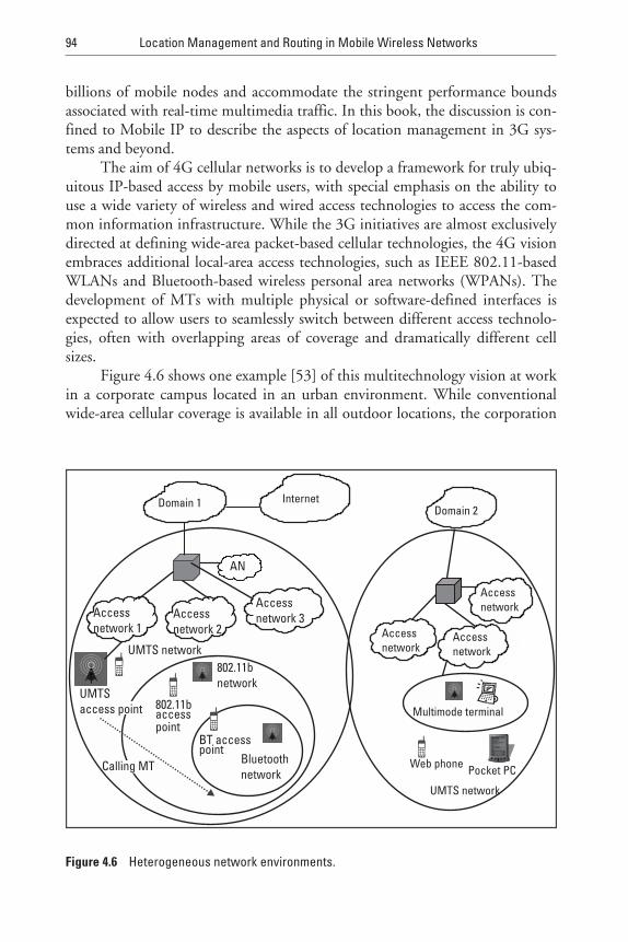
billions of mobile nodes and accommodate the stringent performance boundsassociated with real-time multimedia traffic. In this book, the discussion is con-fined to Mobile IP to describe the aspects of location management in 3G sys-tems and beyond.

The aim of 4G cellular networks is to develop a framework for truly ubiq-uitous IP-based access by mobile users, with special emphasis on the ability touse a wide variety of wireless and wired access technologies to access the com-mon information infrastructure. While the 3G initiatives are almost exclusivelydirected at defining wide-area packet-based cellular technologies, the 4G visionembraces additional local-area access technologies, such as IEEE 802.11-basedWLANs and Bluetooth-based wireless personal area networks (WPANs). Thedevelopment of MTs with multiple physical or software-defined interfaces isexpected to allow users to seamlessly switch between different access technolo-gies, often with overlapping areas of coverage and dramatically different cellsizes.

Figure 4.6 shows one example [53] of this multitechnology vision at workin a corporate campus located in an urban environment. While conventionalwide-area cellular coverage is available in all outdoor locations, the corporation


AN

UMTS network

UMTSaccess point

802.11bnetwork

pointaccess802.11b

Bluetoothnetwork

pointBT access

Calling MT

Domain 1Domain 2

Internet

Accessnetwork

Accessnetwork

Accessnetwork

Accessnetwork 3Access

network 2Accessnetwork 1

UMTS network

Web phone

Multimode terminal

Pocket PC

Figure 4.6 Heterogeneous network environments.

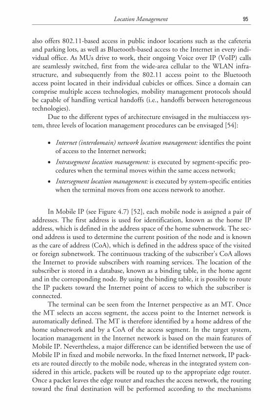
also offers 802.11-based access in public indoor locations such as the cafeteriaand parking lots, as well as Bluetooth-based access to the Internet in every indi-vidual office. As MUs drive to work, their ongoing Voice over IP (VoIP) callsare seamlessly switched, first from the wide-area cellular to the WLAN infra-structure, and subsequently from the 802.11 access point to the Bluetoothaccess point located in their individual cubicles or offices. Since a domain cancomprise multiple access technologies, mobility management protocols shouldbe capable of handling vertical handoffs (i.e., handoffs between heterogeneoustechnologies).

Due to the different types of architecture envisaged in the multiaccess sys-tem, three levels of location management procedures can be envisaged [54]:

• Internet (interdomain) network location management: identifies the pointof access to the Internet network;

• Intrasegment location management: is executed by segment-specific pro-cedures when the terminal moves within the same access network;

• Intersegment location management: is executed by system-specific entitieswhen the terminal moves from one access network to another.

In Mobile IP (see Figure 4.7) [52], each mobile node is assigned a pair ofaddresses. The first address is used for identification, known as the home IPaddress, which is defined in the address space of the home subnetwork. The sec-ond address is used to determine the current position of the node and is knownas the care of address (CoA), which is defined in the address space of the visitedor foreign subnetwork. The continuous tracking of the subscriber’s CoA allowsthe Internet to provide subscribers with roaming services. The location of thesubscriber is stored in a database, known as a binding table, in the home agentand in the corresponding node. By using the binding table, it is possible to routethe IP packets toward the Internet point of access to which the subscriber isconnected.

The terminal can be seen from the Internet perspective as an MT. Oncethe MT selects an access segment, the access point to the Internet network isautomatically defined. The MT is therefore identified by a home address of thehome subnetwork and by a CoA of the access segment. In the target system,location management in the Internet network is based on the main features ofMobile IP. Nevertheless, a major difference can be identified between the use ofMobile IP in fixed and mobile networks. In the fixed Internet network, IP pack-ets are routed directly to the mobile node, whereas in the integrated system con-sidered in this article, packets will be routed up to the appropriate edge router.Once a packet leaves the edge router and reaches the access network, the routingtoward the final destination will be performed according to the mechanisms


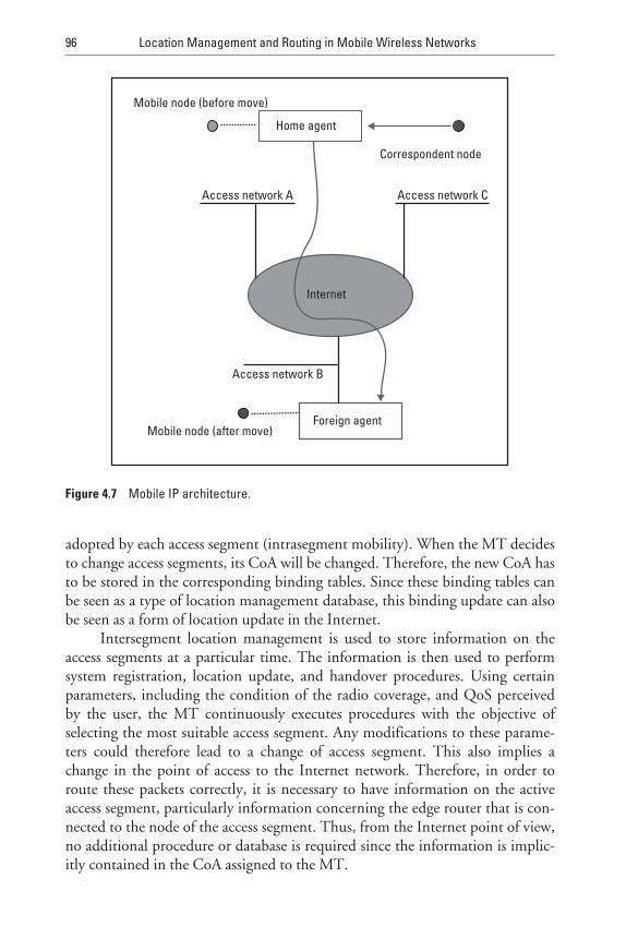
adopted by each access segment (intrasegment mobility). When the MT decidesto change access segments, its CoA will be changed. Therefore, the new CoA hasto be stored in the corresponding binding tables. Since these binding tables canbe seen as a type of location management database, this binding update can alsobe seen as a form of location update in the Internet.

Intersegment location management is used to store information on theaccess segments at a particular time. The information is then used to performsystem registration, location update, and handover procedures. Using certainparameters, including the condition of the radio coverage, and QoS perceivedby the user, the MT continuously executes procedures with the objective ofselecting the most suitable access segment. Any modifications to these parame-ters could therefore lead to a change of access segment. This also implies achange in the point of access to the Internet network. Therefore, in order toroute these packets correctly, it is necessary to have information on the activeaccess segment, particularly information concerning the edge router that is con-nected to the node of the access segment. Thus, from the Internet point of view,no additional procedure or database is required since the information is implic-itly contained in the CoA assigned to the MT.


Internet

Mobile node (before move)

Access network A Access network C

Access network B

Home agent

Foreign agentMobile node (after move)

Correspondent node

Figure 4.7 Mobile IP architecture.

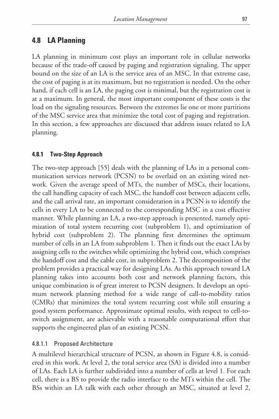
4.8 LA Planning

LA planning in minimum cost plays an important role in cellular networksbecause of the trade-off caused by paging and registration signaling. The upperbound on the size of an LA is the service area of an MSC. In that extreme case,the cost of paging is at its maximum, but no registration is needed. On the otherhand, if each cell is an LA, the paging cost is minimal, but the registration cost isat a maximum. In general, the most important component of these costs is theload on the signaling resources. Between the extremes lie one or more partitionsof the MSC service area that minimize the total cost of paging and registration.In this section, a few approaches are discussed that address issues related to LAplanning.

4.8.1 Two-Step Approach

The two-step approach [55] deals with the planning of LAs in a personal com-munication services network (PCSN) to be overlaid on an existing wired net-work. Given the average speed of MTs, the number of MSCs, their locations,the call handling capacity of each MSC, the handoff cost between adjacent cells,and the call arrival rate, an important consideration in a PCSN is to identify thecells in every LA to be connected to the corresponding MSC in a cost effectivemanner. While planning an LA, a two-step approach is presented, namely opti-mization of total system recurring cost (subproblem 1), and optimization ofhybrid cost (subproblem 2). The planning first determines the optimumnumber of cells in an LA from subproblem 1. Then it finds out the exact LAs byassigning cells to the switches while optimizing the hybrid cost, which comprisesthe handoff cost and the cable cost, in subproblem 2. The decomposition of theproblem provides a practical way for designing LAs. As this approach toward LAplanning takes into accounts both cost and network planning factors, thisunique combination is of great interest to PCSN designers. It develops an opti-mum network planning method for a wide range of call-to-mobility ratios(CMRs) that minimizes the total system recurring cost while still ensuring agood system performance. Approximate optimal results, with respect to cell-to-switch assignment, are achievable with a reasonable computational effort thatsupports the engineered plan of an existing PCSN.

4.8.1.1 Proposed Architecture

A multilevel hierarchical structure of PCSN, as shown in Figure 4.8, is consid-ered in this work. At level 2, the total service area (SA) is divided into a numberof LAs. Each LA is further subdivided into a number of cells at level 1. For eachcell, there is a BS to provide the radio interface to the MTs within the cell. TheBSs within an LA talk with each other through an MSC, situated at level 2,


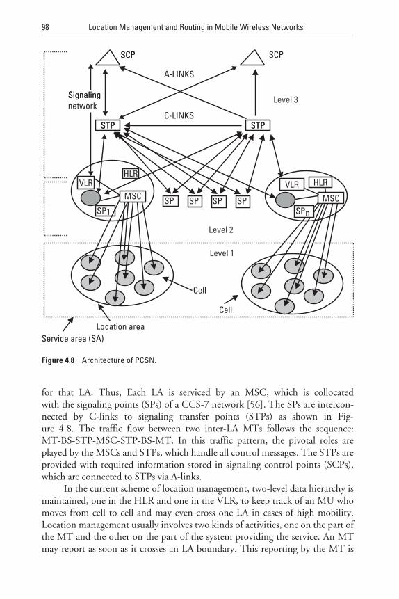
for that LA. Thus, Each LA is serviced by an MSC, which is collocatedwith the signaling points (SPs) of a CCS-7 network [56]. The SPs are intercon-nected by C-links to signaling transfer points (STPs) as shown in Fig-ure 4.8. The traffic flow between two inter-LA MTs follows the sequence:MT-BS-STP-MSC-STP-BS-MT. In this traffic pattern, the pivotal roles areplayed by the MSCs and STPs, which handle all control messages. The STPs areprovided with required information stored in signaling control points (SCPs),which are connected to STPs via A-links.

In the current scheme of location management, two-level data hierarchy ismaintained, one in the HLR and one in the VLR, to keep track of an MU whomoves from cell to cell and may even cross one LA in cases of high mobility.Location management usually involves two kinds of activities, one on the part ofthe MT and the other on the part of the system providing the service. An MTmay report as soon as it crosses an LA boundary. This reporting by the MT is


STPSTP STPSTP

MSC MSCSP SP SP SPSP1

Cell

Location area

SCPSCP SCP

A-LINKS

C-LINKS

SignalingSignalingnetwork

Level 3

Level 2

VLR HLRVLRHLR

Cell

Level 1

Service area (SA)

SPn

Figure 4.8 Architecture of PCSN.

called LU. Understandably, the higher the rate of cell crossing is, the greater thenumber of handoffs and LUs is. Consequently, the updating cost in locationregistration databases increases. In one way, reducing the number of handoffs(in case of uniform traffic distribution and identical cells) can be done by simplyincreasing the cell size. In the worst case, we can make the LA equal to the SA.Enlargement of cell size, however, is limited by the propagation characteristicsand the number of available channels. Moreover, there is another constraint interms of the call handling capacity of an MSC. In order to route an incomingcall to an MT, its location with respect to the PCSN needs to be determinedwithin a fixed time (delay constraint). Therefore, the system can initiate thesearch for the called MT, termed as paging, by simultaneously polling all thecells in case the allowable delay is one polling cycle.

As the size of the LA increases, the cost of paging will also increase as morecells are to be paged to find a called MT. On the other hand, reducing the size ofan LA will increase the number of crossings per unit time. Hence, the cost oflocation update or registration will rise. Both paging and location updates con-sume scarce resources like wireless network bandwidth and power of MTs. Eachhas a significant cost associated with it. So, LA planning is to be based on a crite-rion that guarantees the total signaling load, which comprises paging and regis-tration, is kept under tolerable limits. Therefore, it is characterized by thetrade-off between the number of location updates and the amount of paging sig-naling that the PCSN has to deal with.

4.8.1.2 Methodology Used in the Two-Step Approach

As many variables and complicated constraints are involved in LA design,the method is decomposed into subproblems, namely (1) determination of opti-mum number of cells per LA, and (2) identification of the cells to be connectedto an MSC.

Mobility Model of MTs

Since PCSN is becoming increasingly popular, there is a need for mathematicalmodels to help understand the dynamics and analyze the performance of aPCSN. To simulate the movement of MTs there are several generic models (dis-cussed in Chapter 2) such as the fluid flow model, diffusion model, gravitymodel, and random walk model. This design is independent of the mobilitymodel used for the purpose of analysis. This approach, for the sake of simplicity,considers the fluid flow model to simulate the mobility of the roving MTs tocapture the macroscopic movement behavior.

The fluid flow model assumes that the MTs are uniformly distributed onthe surface of the cell, MTs arrive and depart an LA as a continuous flow offluid, and direction of their movement is uniformly distributed over [0, 2π]. Ifan MT enters a cell at time zero, the initial location of the MT at time zero is


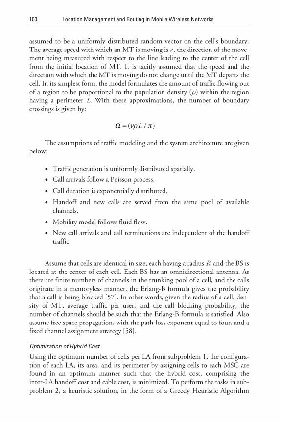
assumed to be a uniformly distributed random vector on the cell’s boundary.The average speed with which an MT is moving is ν, the direction of the move-ment being measured with respect to the line leading to the center of the cellfrom the initial location of MT. It is tacitly assumed that the speed and thedirection with which the MT is moving do not change until the MT departs thecell. In its simplest form, the model formulates the amount of traffic flowing outof a region to be proportional to the population density (ρ) within the regionhaving a perimeter L. With these approximations, the number of boundarycrossings is given by:

Ω = ( / )νρ πL

The assumptions of traffic modeling and the system architecture are givenbelow:

• Traffic generation is uniformly distributed spatially.

• Call arrivals follow a Poisson process.

• Call duration is exponentially distributed.

• Handoff and new calls are served from the same pool of availablechannels.

• Mobility model follows fluid flow.

• New call arrivals and call terminations are independent of the handofftraffic.

Assume that cells are identical in size; each having a radius R, and the BS islocated at the center of each cell. Each BS has an omnidirectional antenna. Asthere are finite numbers of channels in the trunking pool of a cell, and the callsoriginate in a memoryless manner, the Erlang-B formula gives the probabilitythat a call is being blocked [57]. In other words, given the radius of a cell, den-sity of MT, average traffic per user, and the call blocking probability, thenumber of channels should be such that the Erlang-B formula is satisfied. Alsoassume free space propagation, with the path-loss exponent equal to four, and afixed channel assignment strategy [58].

Optimization of Hybrid Cost

Using the optimum number of cells per LA from subproblem 1, the configura-tion of each LA, its area, and its perimeter by assigning cells to each MSC arefound in an optimum manner such that the hybrid cost, comprising theinter-LA handoff cost and cable cost, is minimized. To perform the tasks in sub-problem 2, a heuristic solution, in the form of a Greedy Heuristic Algorithm


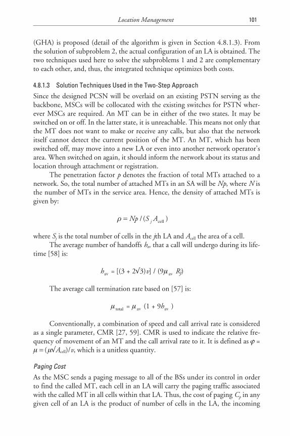
(GHA) is proposed (detail of the algorithm is given in Section 4.8.1.3). Fromthe solution of subproblem 2, the actual configuration of an LA is obtained. Thetwo techniques used here to solve the subproblems 1 and 2 are complementaryto each other, and, thus, the integrated technique optimizes both costs.

4.8.1.3 Solution Techniques Used in the Two-Step Approach

Since the designed PCSN will be overlaid on an existing PSTN serving as thebackbone, MSCs will be collocated with the existing switches for PSTN wher-ever MSCs are required. An MT can be in either of the two states. It may beswitched on or off. In the latter state, it is unreachable. This means not only thatthe MT does not want to make or receive any calls, but also that the networkitself cannot detect the current position of the MT. An MT, which has beenswitched off, may move into a new LA or even into another network operator’sarea. When switched on again, it should inform the network about its status andlocation through attachment or registration.

The penetration factor p denotes the fraction of total MTs attached to anetwork. So, the total number of attached MTs in an SA will be Np, where N isthe number of MTs in the service area. Hence, the density of attached MTs isgiven by:

ρ =Np S Aj/ ( )cell

where Sj is the total number of cells in the jth LA and Acell the area of a cell.The average number of handoffs hav that a call will undergo during its life-

time [58] is:

hav = [(3 + 2√3)v] / (9µav Rj)

The average call termination rate based on [57] is:

µ total = µav (1 + 9hav )

Conventionally, a combination of speed and call arrival rate is consideredas a single parameter, CMR [27, 59]. CMR is used to indicate the relative fre-quency of movement of an MT and the call arrival rate to it. It is defined as ϕ =µ µ= ( √Acell)/v, which is a unitless quantity.

Paging Cost

As the MSC sends a paging message to all of the BSs under its control in orderto find the called MT, each cell in an LA will carry the paging traffic associatedwith the called MT in all cells within that LA. Thus, the cost of paging Cp in anygiven cell of an LA is the product of number of cells in the LA, the incoming


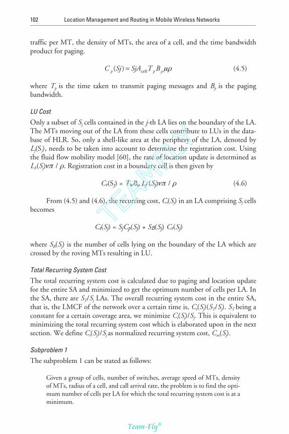
traffic per MT, the density of MTs, the area of a cell, and the time bandwidthproduct for paging.

C Sj SjA T Bp p p( ) = cell µρ (4.5)

where Tp is the time taken to transmit paging messages and Bp is the pagingbandwidth.

LU Cost

Only a subset of Sj cells contained in the j-th LA lies on the boundary of the LA.The MTs moving out of the LA from these cells contribute to LUs in the data-base of HLR. So, only a shell-like area at the periphery of the LA, denoted byLf(Sj), needs to be taken into account to determine the registration cost. Usingthe fluid flow mobility model [60], the rate of location update is determined asLF(Sj)νπ ρ/ . Registration cost in a boundary cell is then given by

Cr(Sj) = TuBu Lf (Sj)νπ ρ/ (4.6)

From (4.5) and (4.6), the recurring cost, Ct(Sj) in an LA comprising Sj cellsbecomes

Ct(Sj) = SjCp(Sj) + SB(Sj) Cr(Sj)

where SB(Sj) is the number of cells lying on the boundary of the LA which arecrossed by the roving MTs resulting in LU.

Total Recurring System Cost

The total recurring system cost is calculated due to paging and location updatefor the entire SA and minimized to get the optimum number of cells per LA. Inthe SA, there are ST/Sj LAs. The overall recurring system cost in the entire SA,that is, the LMCF of the network over a certain time is, Ct(Sj)(ST/Sj). ST being aconstant for a certain coverage area, we minimize Ct(Sj)/Sj. This is equivalent tominimizing the total recurring system cost which is elaborated upon in the nextsection. We define Ct(Sj)/Sj as normalized recurring system cost, Cnt(Sj).

Subproblem 1

The subproblem 1 can be stated as follows:

Given a group of cells, number of switches, average speed of MTs, densityof MTs, radius of a cell, and call arrival rate, the problem is to find the opti-mum number of cells per LA for which the total recurring system cost is at aminimum.


TEAMFLY

Team-Fly®

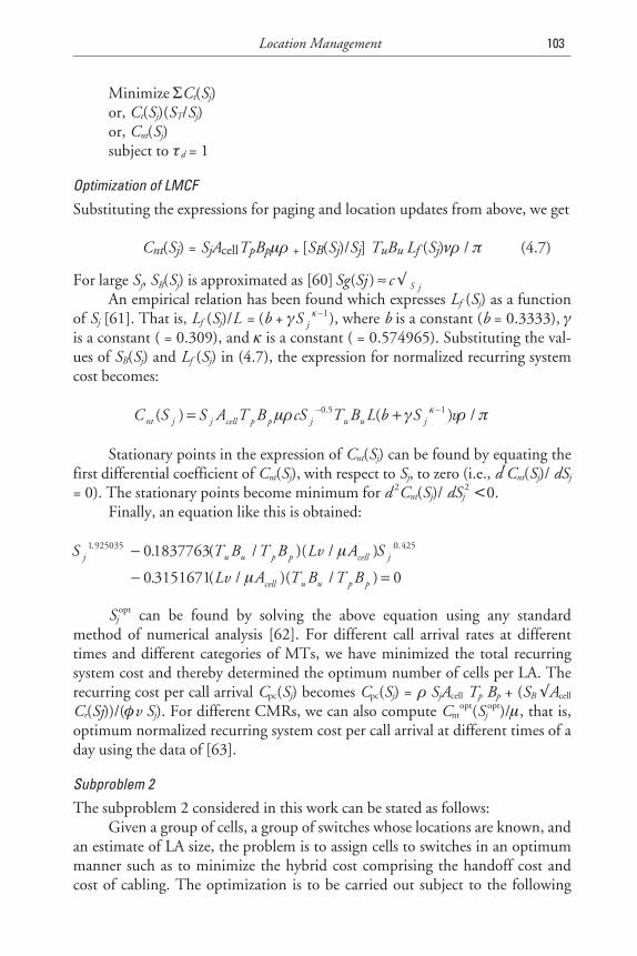
MinimizeΣCt(Sj)or, Ct(Sj)(ST/Sj)or, Cnt(Sj)subject to τd = 1

Optimization of LMCF

Substituting the expressions for paging and location updates from above, we get

Cnt(Sj) = SjAcellTpBpµρ + [SB(Sj)/Sj] TuBu Lf (Sj)νρ π/ (4.7)

For large Sj, SB(Sj) is approximated as [60]Sg Sj c S j( ) ≈ √An empirical relation has been found which expresses Lf (Sj) as a function

of Sj [61]. That is, Lf (Sj)/L = (b + γ κS j−1), where b is a constant (b = 0.3333), γ

is a constant ( = 0.309), and κ is a constant ( = 0.574965). Substituting the val-ues of SB(Sj) and Lf (Sj) in (4.7), the expression for normalized recurring systemcost becomes:

C S S A T B cS T B L b S vnt j j cell p p j u u j( ) ( ) /.= +− −µρ γ ρ πκ0 5 1

Stationary points in the expression of Cnt(Sj) can be found by equating thefirst differential coefficient of Cnt(Sj), with respect to Sj, to zero (i.e., d*Cnt(Sj)/ dSj

= 0). The stationary points become minimum for d 2Cnt(Sj)/ dSj2 <0.

Finally, an equation like this is obtained:

S T B T B Lv A Sj u u p p cell j1 925035 0 42501837763. .. ( / )( / )−

−

µ

0 3151671 0. ( / )( / )Lv A T B T Bcell u u p pµ =

Sjopt can be found by solving the above equation using any standard

method of numerical analysis [62]. For different call arrival rates at differenttimes and different categories of MTs, we have minimized the total recurringsystem cost and thereby determined the optimum number of cells per LA. Therecurring cost per call arrival Cpc(Sj) becomes Cpc(Sj) = ρ SjAcell Tp Bp + (SB √Acell

Cr(Sj))/(φv Sj). For different CMRs, we can also compute Cntopt(Sj

opt)/µ, that is,optimum normalized recurring system cost per call arrival at different times of aday using the data of [63].

Subproblem 2

The subproblem 2 considered in this work can be stated as follows:Given a group of cells, a group of switches whose locations are known, and

an estimate of LA size, the problem is to assign cells to switches in an optimummanner such as to minimize the hybrid cost comprising the handoff cost andcost of cabling. The optimization is to be carried out subject to the following


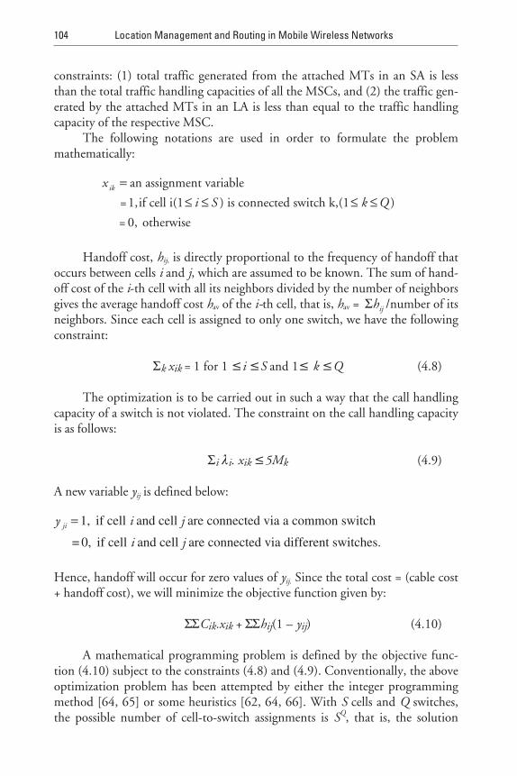
constraints: (1) total traffic generated from the attached MTs in an SA is lessthan the total traffic handling capacities of all the MSCs, and (2) the traffic gen-erated by the attached MTs in an LA is less than equal to the traffic handlingcapacity of the respective MSC.

The following notations are used in order to formulate the problemmathematically:

x

i Sik =

≤ ≤an assignment variable

=1,if cell i(1 ) is connected switch k,(1 )

= 0, otherwise

≤ ≤k Q

Handoff cost, hij, is directly proportional to the frequency of handoff thatoccurs between cells i and j, which are assumed to be known. The sum of hand-off cost of the i-th cell with all its neighbors divided by the number of neighborsgives the average handoff cost hav of the i-th cell, that is, hav = Σhij /number of itsneighbors. Since each cell is assigned to only one switch, we have the followingconstraint:

Σk xik = 1 for 1 ≤i ≤S and 1≤ k ≤Q (4.8)

The optimization is to be carried out in such a way that the call handlingcapacity of a switch is not violated. The constraint on the call handling capacityis as follows:

Σi λi. xik ≤5Mk (4.9)

A new variable yij is defined below:

y i jji = 1, if cell and cell are connected via a common switch

= 0, if cell and cell are connectedi j via different switches.

Hence, handoff will occur for zero values of yij. Since the total cost = (cable cost+ handoff cost), we will minimize the objective function given by:

ΣΣCik.xik + ΣΣhij(1 – yij) (4.10)

A mathematical programming problem is defined by the objective func-tion (4.10) subject to the constraints (4.8) and (4.9). Conventionally, the aboveoptimization problem has been attempted by either the integer programmingmethod [64, 65] or some heuristics [62, 64, 66]. With S cells and Q switches,the possible number of cell-to-switch assignments is SQ, that is, the solution


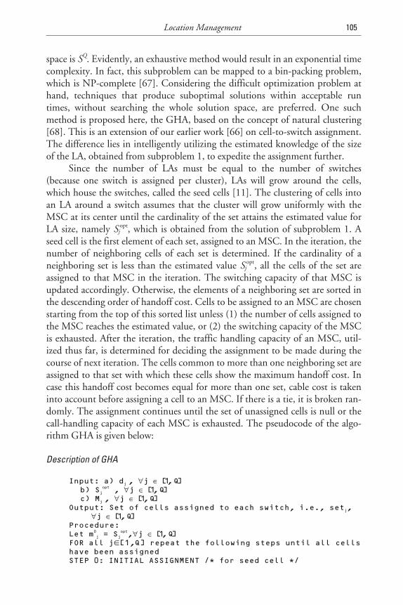
space is SQ. Evidently, an exhaustive method would result in an exponential timecomplexity. In fact, this subproblem can be mapped to a bin-packing problem,which is NP-complete [67]. Considering the difficult optimization problem athand, techniques that produce suboptimal solutions within acceptable runtimes, without searching the whole solution space, are preferred. One suchmethod is proposed here, the GHA, based on the concept of natural clustering[68]. This is an extension of our earlier work [66] on cell-to-switch assignment.The difference lies in intelligently utilizing the estimated knowledge of the sizeof the LA, obtained from subproblem 1, to expedite the assignment further.

Since the number of LAs must be equal to the number of switches(because one switch is assigned per cluster), LAs will grow around the cells,which house the switches, called the seed cells [11]. The clustering of cells intoan LA around a switch assumes that the cluster will grow uniformly with theMSC at its center until the cardinality of the set attains the estimated value forLA size, namely Sj

opt, which is obtained from the solution of subproblem 1. Aseed cell is the first element of each set, assigned to an MSC. In the iteration, thenumber of neighboring cells of each set is determined. If the cardinality of aneighboring set is less than the estimated value Sj

opt, all the cells of the set areassigned to that MSC in the iteration. The switching capacity of that MSC isupdated accordingly. Otherwise, the elements of a neighboring set are sorted inthe descending order of handoff cost. Cells to be assigned to an MSC are chosenstarting from the top of this sorted list unless (1) the number of cells assigned tothe MSC reaches the estimated value, or (2) the switching capacity of the MSCis exhausted. After the iteration, the traffic handling capacity of an MSC, util-ized thus far, is determined for deciding the assignment to be made during thecourse of next iteration. The cells common to more than one neighboring set areassigned to that set with which these cells show the maximum handoff cost. Incase this handoff cost becomes equal for more than one set, cable cost is takeninto account before assigning a cell to an MSC. If there is a tie, it is broken ran-domly. The assignment continues until the set of unassigned cells is null or thecall-handling capacity of each MSC is exhausted. The pseudocode of the algo-rithm GHA is given below:

Description of GHA

Input: a) dj , ∀ ∈j Q[, ]1b) Sj

opt , ∀ ∈j Q[, ]1c) Mj , ∀ ∈j Q[, ]1

Output: Set of cells assigned to each switch, i.e., setj,∀ ∈j Q[, ]1

Procedure:Let m0

j = Sj

opt,∀ ∈j Q[, ]1FOR all j∈[1,Q] repeat the following steps until all cellshave been assignedSTEP 0: INITIAL ASSIGNMENT /* for seed cell */


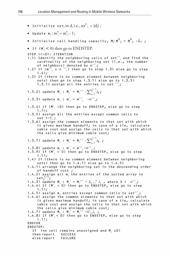
• Initialize setj to dj i.e., set0j = dj ;

• Update mj : m0j = m0

j - 1;

• Initialize call handling capacity, Mj: M0j = M

0j -λi ;

• If (Mij < 0) then go to ENDSTEP.

STEP i(>0): ITERATIONi.1) Identify the neighboring cells of seti-1

j and find thecardinality of the neighboring set (i.e., the numberof neighbors) denoted by ni-1

j;i.2) If (mi-1

j ≥ n i-1

j) then go to step i.3) else go to stepi.4);

i.3) If (there is no common element between neighboringsets) then go to step i.3.1) else go to i.3.5)i.3.1) assign all the entries to set i-1

j;

i.3.2) update Mj : Mj

i = Mj

i-1 −=

−

∑ λkn

k

ji

1

1

;

i.3.3) update mj : mi

j = mi-1

j -ni-1

j;

i.3.4) If (Mi

j <0) then go to ENDSTEP, else go to stepi.1);

i.3.5) assign all the entries except common cells toset i-1j ;

i.3.6) assign the common elements to that set with whichit gives maximum handoff; in case of a tie, calculatecable cost and assign the cells to that set with whichthe cells give minimum cable cost;


i = Mj

i-1 −=

−

∑ λkn

k

ji

1

1

;

i.3.8) update mj : mi

j = mi-1

j -ni-1

j ;i.3.9) If (Mi

j < 0) then go to ENDSTEP, else go to stepi.1);

i.4) If (there is no common element between neighboringsets) then go to i.4.1) else go to i.4.5)

i.4.1) arrange the neighboring set in the descending orderof handoff cost ;

i.4.2) assign all mj the entries of the sorted array tosetj

i−1;i.4.3) update Mj : Mj

i = Mj

i-1 - Σk = 1

X λk , where X = ni-1

j;i.4.4) If (Mi


i.4.5) assign mj entries except common cells to seti-1

j;i.4.6) assign the common elements to that set with which

it gives maximum handoff; in case of a tie, calculatecable cost and assign the cells to that set with whichthe cells give minimum cable cost;


i = Mj

i-1 -Σx

κ=1λk ;i.4.8) If (Mi


ENDFORENDSTEP:

If (no cell remains unassigned and Mj ≥0)then report SUCCESSelse report FAILURE


In order to design a feasible PCSN, constraints like traffic-handling capac-ity of MSCs and costs related to paging, registration, and cabling should be con-sidered. Utilizing the available information of MTs and the network in asuitable manner, it is possible to devise a technique for planning LAs in a PCSNthat optimizes both recurring system cost and hybrid cost. With the networkengineering and configuration in mind, the fluid flow mobility model is capableof investigating the performance and cost of signaling traffic.

As this two-step approach toward LA planning takes into account bothcost and network planning factors, this unique combination is of great interestto PCSN designers. It develops an optimum network planning method for awide range of CMRs that minimizes the total recurring system cost while stillensuring good system performance. Approximate optimal results, with respectto cell-to-switch assignment, are achievable with a reasonable computationaleffort. However, an ideal LU and paging mechanism for high values of CMR iswarranted to adjust LA per MT basis.

This design is not restricted to any particular assumption on the mobilitypattern of MTs or the mobility model either. Since, the optimum LA sizedecreases significantly with the increase in CMR, as the corresponding hike insystem cost is very high, design parameters at BSs and MSCs cannot be specifieduntil cell allocation is completed. Finally, channel assignment, which can fur-ther improve system performance in terms of QoS and improved carrier inter-ference ratio, can only be determined once the architecture of the PCSN hasbeen obtained.

4.8.2 LA Planning and Signaling Requirements

In second-generation mobile systems [7], LA planning does not generate signifi-cant problems since the number of generated LUs (as well as the amount of pag-ing signaling) remains relatively low because of the low number of users. For 3Gmobile telecommunication systems, several alternative location-tracking tech-niques have been used (e.g., based on the use of reporting centers or a dynamicLA management protocol). Nevertheless, in UMTS an approach similar to the2G location-finding approach has been used. That is, the system area is dividedinto LAs and a called user is located in two steps: (1) determine the LA withinwhich the user roams, and (2) perform paging within this LA. The main issueconcerning LA planning in 3G mobile telecommunication systems is theamount of location-finding-related signaling load [paging signaling, locationupdating, and distributed database (DDB) queries].

Since the size and shape of an LA affects the signaling requirements due topaging and LU, it is obvious that LA planning should minimize both, if possi-ble. In order to provide a clear view of the relation between the LA planning and


the above-mentioned parameters, we consider two extreme LA planningapproaches:

1. The system area is equal to an LA. Whenever an MT is called, it is pagedover the whole system coverage area, while no LUs are performed dueto MU movements. In this case, paging signaling load can be enor-mous especially during the busy hour.

2. The cell area is equal to an LA. In this case, the location of an MT isdetermined with an accuracy of a single cell area. The need for paginghere is minimal; paging does not locate the MT, it just alerts the termi-nal for the incoming call. The number of Lus, however, is expected tobe enormous due to the small cell size and the user mobility. A briefdescription of the LA planning methods under consideration follows:

a. LA planning based on heuristic algorithms: This is a method to ap-proximate the optimum LA planning as a set of cells. According tothe example heuristic algorithm used in this chapter, cells are ran-domly selected to form LAs.b. LA planning based on area zones and highway topology: Area zonesare defined according to geographical criteria (e.g., city center), andthe approach considers the population distribution and the way thatpeople move via the city highways in order to determine the properLA configuration.c. LA planning based on overlapping LA borders: This method can beconsidered an attempt to improve the previous one by means of re-ducing the number of generated LUs. In this case, LAs have over-lapping borders in order to avoid LUs due to MU movementsaround the LA borders.d. Time-dependent LA configuration: According to this scenario, thenetwork alters the LA configuration based on either some prede-fined timetable or monitoring of the number of LUs and thenumber of paging messages. The LA configuration here is selectedso as to fit the time-variable mobility and traffic conditions.e. LA planning based on MU grouping: This method considers themobility behavior of each individual MU in order to minimize thenumber of LUs generated due to daily MU movements. To applythis method, MUs are grouped based on their mobility behavior(e.g., high-mobility MUs) and a different LA configuration is deter-mined for each group.f. LA planning using simulated annealing [69]: This research, focus-ing on LA management in wireless cellular networks, has minimizedthe total paging and registration cost. This chapter finds an optimal


method for determining the LAs. To that end, an appropriate ob-jective function is defined with the addition of paging and registra-tion costs. For that purpose, the available network information toformulate a realistic optimization problem is used. In reality, theload (i.e., cost) of paging and registration to the network variesfrom cell to cell. An algorithm based on simulated annealing for thesolution of the resulting problem is used.

4.9 Conclusion

Location management is a key factor for wireless mobile networks. Without agood strategy for location management, mobile communication and computingcannot exist. Mobile cellular radio networks of the third generation will be usedby an increasing number of users. Thus, location management functions forproviding a continuity of service over the whole system area have to be muchmore sophisticated than in today’s cellular networks.

In this chapter, we have looked at different mechanisms to locate an MT’scurrent network address and discussed their advantages and disadvantages.Location management functions, such as location updating and paging, have tofulfill services and the requirements of users and operators. One of these require-ments is cost efficiency, which could be reached by minimizing the signalingtraffic both on radio links and on fixed network links. What we aim for is a loca-tion management scheme that will provide efficient searches and updates trans-parent to the user.

References

[1] Madhow, U., M. L. Honig, and K. Steiglitz, “Optimization of Wireless Resources for Per-sonal Communications Mobility Tracking,” IEEE/ACM Trans. on Networking, Vol. 3,No. 6, 1995, pp. 698–706.

[2] Ramanathan S., and Martha Steenstrup, “A Survey of Routing Techniques for MobileCommunications Networks,” 1996.

[3] Ketchum, J. W., “Routing in Cellular Mobile Radio Communication Networks,” Routingin Communication Networks, M. Steenstrup (ed.), Englewood Cliffs, NJ: Prentice-Hall,1995.

[4] Mouly, M., and M. B. Pautet, “The GSM System for Mobile Communications,” Palaiseu,France: M. Mouly, 1992.

[5] Telecommunications Industry Association, Cellular Radio Telecommunication Intersys-tem Operation, TIA/EIA IS-41B, 1991.


[6] Mohan, S., and R. Jain, “Two User Location Strategies for Personal CommunicationsServices,” IEEE Personal Communications, First Quarter, 1994, pp. 42–50.

[7] G. L., Markoulidakis, et al., “Evaluation in LA Planning in Future Mobile Telecommuni-cation Systems,” Wireless Network, 1995.

[8] Bar-Noy, A., and I. Kessler, “Tracking Mobile Users in Wireless Communications Net-works,” IEEE Trans. on Information Theory, Vol. 39, No. 6, 1993, pp. 1877–1886.

[9] Xie, H., S. Tabbane, and D. J. Goodman, “Dynamic Location Area Management and Per-formance Analysis,” Proc. 43rd IEEE Vehicular Tech. Conf., 1993, pp. 536–539.

[10] Birk Y., and Y. Nachman, “Using Direction and Elapsed-Time Information to Reduce theWireless Cost of Locating Mobile Units in Cellular Networks,” Wireless Networks, Vol. 1,No. 4, 1995, pp. 403–412.

[11] Bar-Noy, A., I. Kessler, and M. Sidi, “Mobile Users: To Update or Not To Update?”Wireless Networks, Vol. 1, No. 2, 1995, pp. 175–186.

[12] Rose, C., and R. Yates, “Minimizing the Average Cost of Paging Under Delay Con-straints,” Wireless Networks, Vol. 1, Feb. 1995, pp. 211–219.

[13] Akyildiz, Ian F., and Joseph S. M. Ho, “A Mobile User Location Update and PagingMechanism Under Delay Constraints, Proc. of ACM SIGCOMM, Cambridge, MA, 1995,pp. 244–255.

[14] IETF Mobile-IP Working Group, IPv4 Mobility Support, working draft, 1995.

[15] Meier-Hellstern, K., and E. Alonso, “The Use of SS7 and GSM to Support High DensityPersonal Communications,” Proc. of ICC, 1992, pp. 1698–1702.

[16] Lo, V. N., R. S. Wolf, and R. C. Bernhardt, “Expected Network Database TransactionVolume to Support Personal Communications Services,” 1st International Conference Uni-versal Personal Communications Services, Dallas, TX, 1992.

[17] Jain, R., et al., “A Caching Strategy To Reduce Network Impacts of PCS,” IEEE J. onSelected Areas in Communications, Vol. 12, No. 8, 1994, pp. 1434–1444.

[18] Ho, J. S. M., and I. F. Akyildiz, “Local Anchor Scheme for Reducing Location TrackingCosts in PCNs,” Proc. of ACM MOBICOM, Berkeley, CA, 1995, pp. 181–194.

[19] Awerbuch, B., and D. Peleg, “Concurrent Online Tracking of Mobile Users,” Proc. ofACM SIGCOMM, Zurich, Switzerland, 1991, pp. 221–234.

[20] Anantharam, V., et al, “Optimization of a Database Hierarchy for Mobility Tracking in aPersonal Communications Network,” Performance Evaluation, Vol. 20, 1994,pp. 287–300.

[21] Badrinath, B. R., T. Imielinski, and A. Virmani, “Locating Strategies for Personal Com-munication Networks,” Proc. of Workshop on Networking of Personal CommunicationsApplications, 1992.

[22] Ozsu, M. T., and P. Valduriez, “Principles of Distributed Systems,” Englewood Cliffs, NJ:Prentice-Hall, 1991.

[23] Dowdy, L. W., and D. V. Foster, “Comparative Models of the File Allocation Problem,”ACM Computing Surveys, Vol. 14, No. 2, 1982, pp. 287–313.


[24] Shivakumar, N., and J. Widom, “User Profile Replication for Faster Location Lookup inMobile Environments,” Proc. of ACM MOBICOM, Berkeley, CA, 1995, pp. 161–169.

[25] Akyildiz, Ian F., and Joseph S. M. Ho, “On Location Management for Personal Commu-nications Networks,” IEEE Communications Magazine, Sept. 1996, pp. 138–45.

[26] Rose, C., “Minimizing the Average Cost of Paging and Registration: A Timer-BasedMethod,” ACM J. Wireless Networks, Feb. 1996, pp. 109–16.

[27] Akyildiz, Ian F., Joseph S. M. Ho, and Yi-Bing Lin, “Movement-Based Location Updateand Selective Paging for PCS Networks,” 1996.

[28] Bar-Noy, A., and I. Kessler, “Mobile Users: To Update or Not To Update?” Proc.INFOCOM 94, June 1994, pp. 570–76.

[29] Lyberopoulos, G. L., et al., “Intelligent Paging Strategies for Third Generation MobileTelecommunication Systems,” IEEE Trans on Vehicular Technology, Aug 1995,pp. 543-53.

[30] Wang, Wenye, Ian F. Akyildiz, and Gordon L. Stüber, “Effective Paging Schemes withDelay Bounds As QoS Constraints in Wireless Systems,” Wireless Networks, Vol. 7, 2001,pp. 455–466.

[31] Bhattacharjee, P. S., D. Saha, and A. Mukherjee, “Paging Strategies for Future PersonalCommunication Services Networks,” Proc 6th Int. Conf. on High Performance Computing(HiPC’99), Calcutta, India, Dec. 1999.

[32] Papoulis, A., Probability, Random Variable, and Stochastic Processes, 3rd Edition, NewYork: McGraw Hill, 1991.

[33] Wang, Wenye, Ian F. Akyildiz, and Gordon L. Stüber, “Reducing the Paging Costs UnderDelay Bounds for PCS Networks,” Proc. of IEEE WCNC’2000, Sept. 2000.

[34] Akyildiz, Ian F., and Wenye Wang, “A Dynamic Location Management Scheme forNext-Generation Multitier PCS Systems,” IEEE Transactions on Wireless Communications,Jan. 2002.

[35] Sarikaya, Behcet, and Sridhar Gurivireddy, “Evaluation of CDMA2000 Support for IPMicromobility Handover and Paging Protocols,” IEEE Communications Magazine, May2002, pp. 146–149.

[36] Kempf, J., et al., “Requirements for Layer 2 Protocols to Support Optimized Handoverfor IP Mobility,” IETF Draft, July 2001.

[37] Kempf, J., et al., “Bidirectional Edge Tunnel Handover for IPv6,” IETF draft, Sept. 2001.

[38] Gurivireddy, S., B. Sarikaya, and A. Krywaniuk, “Layer-2 Aided Mobility IndependentDormant Host Alerting Protocol,” IETF draft, Sept. 2001.

[39] EIA/TIA, “Cellular Radio-Telecommunications Intersystem Operations,” Tech. Rep.IS-41 Revision C, 1995.

[40] Tabbane, Sami, “Location Management Methods for Third-Generation Mobile Systems,”IEEE Communications Magazine, Aug. 1997, pp. 72–84.

[41] Lee, W. C. Y., Mobile Cellular Telecommunications Systems, New York: McGraw-Hill,1989.


[42] Wang, D. C. C., “A Survey of Number Mobility Techniques for PCS,” Proc. IEEE Int.Conf. On Personal Communications, Tokyo, Japan, Nov. 6–10, 1995.

[43] Wang, D. C. C., “A Survey of Number Mobility Techniques for PCS,” Proc. IEEE ICC,1994.

[44] Tabbane, S., “Database Architectures and Location Strategies for Mobility Managementin Mobile Radio Systems,” Proc. Wksp. Multiaccess, Mobility and Teletraffic for Persona.Communications, Paris, France, May 1996.

[45] Jabbari, B., “Intelligent Network Concepts in Mobile Communications,” IEEE Communi-cation Magazine, Feb. 1992.

[46] Plassmann, D., “Location Management for MBS,” Proc. IEEE VTC, Stockholm, Sweden,June 8–10, 1994, pp. 649–53.

[47] Okasaka, S., et al., “A New Location Updating Method for Digital Cellular Systems,”Proc. IEEE VTC ’91, Saint Louis, MI, May 1991.

[48] Hu, L. R. and S. S. Rappaport, “An Adaptive Location Management Scheme for GlobalPersonal Communications,” Proc. IEEE Int. Conf. On Personal Communications, Tokyo,Japan, Nov. 6–10, 1995.

[49] RACE II Deliverable, “Location Areas, Paging Areas and the Network Architecture,”R2066/PTTNL/MF1/DS/P/001/b1, Apr. 1992.

[50] Tabbane, S., “Comparison between the Alternative Location Strategy (AS) and the Classi-cal Location Strategy (CS),” WINLAB Tech. Rep. 37, Aug. 1992.

[51] Tabbane, S., “An Alternative Strategy for Location Tracking,” IEEE JSAC, Vol. 13, No. 5,June 1995.

[52] Perkins, C., “IP Mobility Support for IPv4, revised,” draft-ietf-mobileip-rfc2002-bis-08.txt,IETF, Sept. 2001.

[53] Misra, Archan, et al., “IDMP-Based Fast Handoffs and Paging in IP-Based 4G MobileNetworks,” IEEE Communications Magazine, March 2002, pp. 138–145.

[54] Chan, P. M. L., et al., “Mobility Management Incorporating Fuzzy Logic for a Heteroge-neous IP Environment,” IEEE Communications Magazine, Dec. 2001, pp. 42–51.

[55] Bhattacharjee, P. S., et al., “A Practical Approach for Location Area Planning in a PersonalCommunication Services Network,” Proceedings of MMT ’98, USA, 1998.

[56] Modarressi, A. R., and R. A. Skoog, “Signaling System No. 7: A Tutorial,” IEEE Commu-nication Magazine, July 1990 pp. 19–35.

[57] Gunz, A., C. M. Krishna, and D. Tang, “On Optimal Design of Multitier Wireless Cellu-lar Systems,” IEEE Communications Magazine, Feb. 1997, pp. 88–93.

[58] Guerin, R., “Channel Occupancy Time Distribution in a Cellular Radio System,” IEEETrans. on Vehicular Tech., Vol. VT-35, No. 3, Aug. 1987.

[59] Chih-Lin, I., P. Pollini, and R. B. Gitlin, “PCS Mobility Management Using Virtual CallSetup Algorithm,” IEEE Trans. on Networking, Vol. 5, No. 1, Feb. 1997.


TEAMFLY

Team-Fly®

[60] Alonso, E., K. S. Hellstern, and G. P. Pollini, “Influence of Cell Geometry on Handoverand Registration Rates in Cellular and Universal Personal Telecomm Networks,” Proc. 8thInt. Teletraffic Seminar, Sonata Marghareta, Ligure, Geneva, Italy.

[61] Bhattacharjee, P. S., D. Saha, and A. Mukherjee, “Heuristics for Assignment of Cells toSwitches in a PCSN: A Comparative Study”, ICPWC’99, Proc. IEEE International Confer-ence Personal Communication, Jaipur, India, 1999, pp. 331–334.

[62] Jain, M. K., S. R. K. Iyengar, and R. K. Jain, Numerical Methods for Scientific and Engi-neering Computation, New York: Wiley Eastern Limited, 1985, pp. 41–43.

[63] Markoulidakis, J. G., G. L. Lyberopolous, and M. E. Anynostom, “Traffic Model forThird-Generation Cellular Mobile Telecomm. Systems,” Wireless Network, 1998.

[64] Merchant, A., and B. Sengupta, “Assignment of Cells to Switches in PCS Networks,”IEEE/ACM Trans. on Networking, Vol. 3, No. 5, Oct. 1995, pp. 521–526.

[65] Nemhauser, G. L., and L. A. Woolly, Integer and Combinatorial Optimization, New York:Wiley, 1988.

[66] Saha, D., A. Mukherjee, and P. S. Bhattacharjee, “A Simple Heuristic for Assignment ofCells to Switches in a PCS Network,” Wireless Personal Communication, Netherlands: Klu-wer Academic Publishers, 2000, pp. 209–224.

[67] Gary M. R., and D. S. Johnson, “Computers and Intractability, A Guide to the Theory ofNP-Completeness,” New York: W. H. Freeman, 1979.

[68] Saha, D., and A. Mukherjee, “Design of Hierarchical Communication Network UnderNode-Link Failure Constraints,” Computer Communication, Vol. 18, No. 5, 1995,pp. 378–383.

[69] Demirkol, Ilker, et al., “Location Area Planning in Cellular Networks Using SimulatedAnnealing,” Proc. of INFOCOM, 2001.


.

Part IIAd Hoc Wireless Networks

.

5Overview

5.1 Characteristics of Ad Hoc Networks

Ad hoc networks have several salient characteristics [1–4]:

• Dynamic topologies: Because of the possibly rapid and unpredictablemovement of the nodes and fast-changing propagation conditions, net-work information, such as link-state, becomes quickly obsolete. Thisleads to frequent network reconfigurations and frequent exchanges ofcontrol information over the wireless medium.

• Asymmetric link characteristics: In a wireless environment, communica-tion between two nodes may not work equally well in both directions.In other words, even if node n is within the transmission range of nodem, the reverse may not be true. Although we have assumed bidirectionallinks in Figure 1.5, some of them may be unidirectional in a real-lifescenario.

• Multihop communication: Each node in an ad hoc network willact as a transmitter, a receiver, or a relay station. So, packetsfrom a transmitter node (source) may reach the receiver node (destina-tion) in multiple hops through several intermediate relay nodes. How-ever, the successful operation of an ad hoc network will be hamperedif an intermediate node, participating in a communication between asource-destination pair, moves out of range suddenly or switches itselfoff in between message transfer. The situation is worse if there is noother path between those two nodes. In Figure 1.5, if D moves out ofrange disconnecting the link between C and D, or if D switches itself

117

off, the communication between C and F would be interrupted. Theabsence of D creates two disconnected components: A, B, C and E,F, G .

• Decentralized operation: Ad hoc networks are network architectures thatcan be rapidly deployed and that do not need to rely on preexistinginfrastructure or centralized control. In cellular wireless networks, thereare a number of centralized entities; (e.g., BSs, MSCs, and the HLR)In ad hoc networks, since there is no preexisting infrastructure, thesecentralized entities do not exist. The centralized entities in the cellu-lar networks perform the function of coordination. Thus, lack of theseentities in the ad hoc networks requires more sophisticated distributedalgorithms to perform equivalent functions.

• Bandwidth-constrained variable-capacity links: Wireless links will con-tinue to have significantly lower capacity than their hardwired coun-ter parts. In addition, the realized throughput of wirelesscommunications is often much less than a radio’s maximum transmis-sion rate because of the effects of multiple access, fading, noise, andinterference conditions, for example. One effect of the relatively low tomoderate link capacities is that congestion is typically the norm ratherthan the exception. Thus, the aggregate application demand will likelyapproach or exceed network capacity frequently. This demand will con-tinue to increase as multimedia computing and collaborative network-ing applications increase.

• Energy-constrained operation: The mobile nodes in an ad hoc networkrely on batteries or other exhaustible means for their energy. For thesenodes, the most important system design criteria for optimization maybe energy conservation. One way of achieving this is to optimize thetransmission power of each node.

These characteristics of ad hoc networks create a set of performance con-cerns for protocol design that extend beyond those guiding the design of proto-cols for conventional networks with preconfigured topology.

5.2 Three Fundamental Design Choices

We focus here on three fundamental choices in the design of ad hoc networks[5]:

1. The network architecture;

2. The routing protocol;

3. The medium access control.


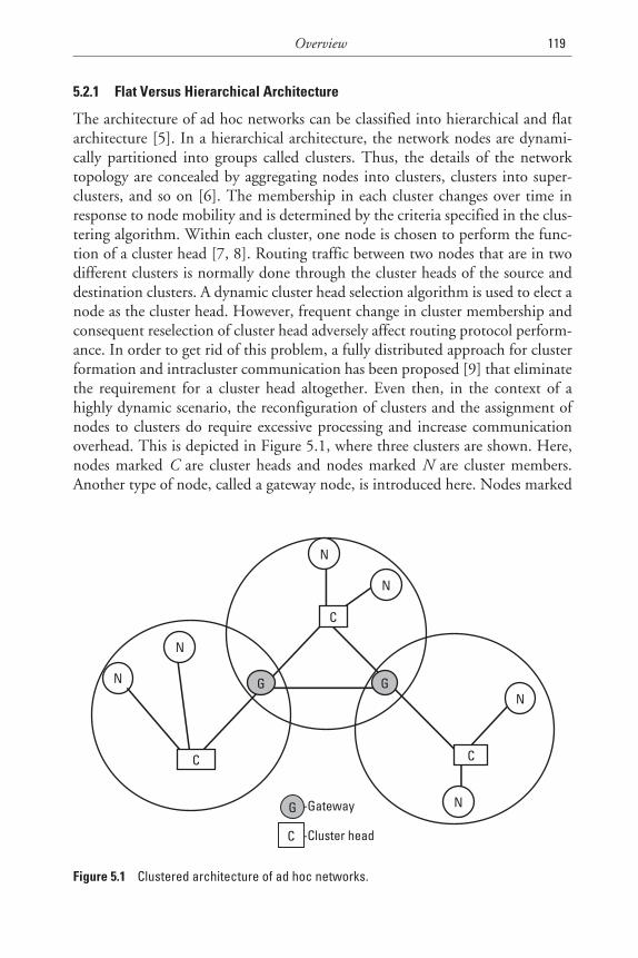
5.2.1 Flat Versus Hierarchical Architecture

The architecture of ad hoc networks can be classified into hierarchical and flatarchitecture [5]. In a hierarchical architecture, the network nodes are dynami-cally partitioned into groups called clusters. Thus, the details of the networktopology are concealed by aggregating nodes into clusters, clusters into super-clusters, and so on [6]. The membership in each cluster changes over time inresponse to node mobility and is determined by the criteria specified in the clus-tering algorithm. Within each cluster, one node is chosen to perform the func-tion of a cluster head [7, 8]. Routing traffic between two nodes that are in twodifferent clusters is normally done through the cluster heads of the source anddestination clusters. A dynamic cluster head selection algorithm is used to elect anode as the cluster head. However, frequent change in cluster membership andconsequent reselection of cluster head adversely affect routing protocol perform-ance. In order to get rid of this problem, a fully distributed approach for clusterformation and intracluster communication has been proposed [9] that eliminatethe requirement for a cluster head altogether. Even then, in the context of ahighly dynamic scenario, the reconfiguration of clusters and the assignment ofnodes to clusters do require excessive processing and increase communicationoverhead. This is depicted in Figure 5.1, where three clusters are shown. Here,nodes marked C are cluster heads and nodes marked N are cluster members.Another type of node, called a gateway node, is introduced here. Nodes marked

Overview 119

G -Gateway

C -Cluster head

C C

C

GG

N

N

N

N

N

N

Figure 5.1 Clustered architecture of ad hoc networks.

G are gateway nodes for intercluster communications. Intracluster communica-tions are done through the respective cluster head. The detailed routing mecha-nism in this type of architecture will be illustrated in Chapter 7.

In contrast, in a flat architecture, there are no clusters and the neighbor-ing nodes can communicate directly. It has been argued that the routing inflat architecture is more optimal (close-by nodes do not have to communicatethrough the hierarchy) and the network tends to better balance the load amongmultiple paths, thus reducing the traffic bottlenecks that occur at the clusternodes in the hierarchical approach [5].

In a hierarchical architecture, some nodes, such as cluster heads andgate way nodes, have a higher computation and communication burden thanother nodes. The network reliability may be affected due to this single point offailure of these critical nodes. However, the routing messages may only haveto propagate within a cluster. Thus, the number of globally propagated rout-ing messages is small. On the contrary, in a flat architecture, all nodes carry thesame responsibility, and reliability is not dependent on any single point of fail-ure. However, this flat architecture is not bandwidth efficient because the rout-ing messages have to propagate globally throughout the network. The scalabilitygets worse when the number of nodes increases.

The main advantage of the hierarchical ad hoc network is the ease of themobility management process. In order to limit far-reaching impact to topol-ogy dynamics, complete routing information is maintained only for intraclusterrouting. Intercluster routing is achieved by hiding the topology details withina cluster from external nodes and using hierarchical aggregation, reactive rout-ing, or a combination of both techniques. Cluster heads can act as a databasesthat contain the location of the nodes in their own clusters. To determine theexistence and the location of a mobile node, a query is broadcasted to all thecluster heads. The cluster under which the node resides, responds to the queryoriginator. A mobility management scheme needs to be implemented in the flatnetworks by appropriate routing algorithms, although it would increase theoverhead due to control message propagation throughout the network [5].

5.2.2 Proactive Versus Reactive Routing

The existing routing protocol can be classified either as proactive or as reactive.In proactive protocols the routing information within the network isalways known beforehand through continuous route updates. The distance vec-tor and link-state protocols are examples of proactive schemes. Examples of pro-active routing methods in an ad hoc network environment are [10, 11].However, these methods require one to know the topology of the entire networkand this information needs to be propagated through the network. As the net-work size increases and as the nodal mobility increases, a smaller and smaller


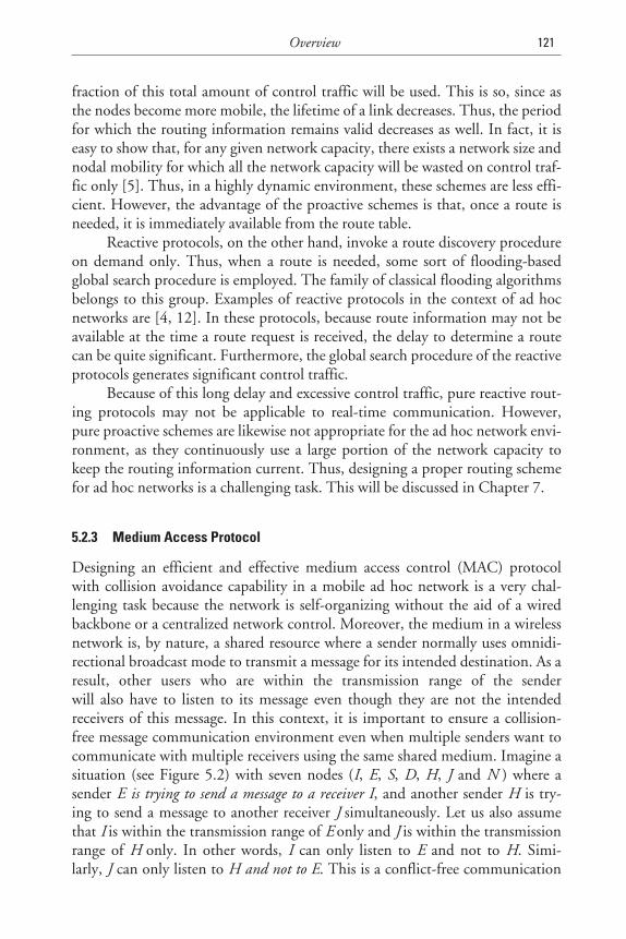
fraction of this total amount of control traffic will be used. This is so, since asthe nodes become more mobile, the lifetime of a link decreases. Thus, the periodfor which the routing information remains valid decreases as well. In fact, it iseasy to show that, for any given network capacity, there exists a network size andnodal mobility for which all the network capacity will be wasted on control traf-fic only [5]. Thus, in a highly dynamic environment, these schemes are less effi-cient. However, the advantage of the proactive schemes is that, once a route isneeded, it is immediately available from the route table.

Reactive protocols, on the other hand, invoke a route discovery procedureon demand only. Thus, when a route is needed, some sort of flooding-basedglobal search procedure is employed. The family of classical flooding algorithmsbelongs to this group. Examples of reactive protocols in the context of ad hocnetworks are [4, 12]. In these protocols, because route information may not beavailable at the time a route request is received, the delay to determine a routecan be quite significant. Furthermore, the global search procedure of the reactiveprotocols generates significant control traffic.

Because of this long delay and excessive control traffic, pure reactive rout-ing protocols may not be applicable to real-time communication. However,pure proactive schemes are likewise not appropriate for the ad hoc network envi-ronment, as they continuously use a large portion of the network capacity tokeep the routing information current. Thus, designing a proper routing schemefor ad hoc networks is a challenging task. This will be discussed in Chapter 7.

5.2.3 Medium Access Protocol

Designing an efficient and effective medium access control (MAC) protocolwith collision avoidance capability in a mobile ad hoc network is a very chal-lenging task because the network is self-organizing without the aid of a wiredbackbone or a centralized network control. Moreover, the medium in a wirelessnetwork is, by nature, a shared resource where a sender normally uses omnidi-rectional broadcast mode to transmit a message for its intended destination. As aresult, other users who are within the transmission range of the senderwill also have to listen to its message even though they are not the intendedreceivers of this message. In this context, it is important to ensure a collision-free message communication environment even when multiple senders want tocommunicate with multiple receivers using the same shared medium. Imagine asituation (see Figure 5.2) with seven nodes (I, E, S, D, H, J and N ) where asender E is trying to send a message to a receiver I, and another sender H is try-ing to send a message to another receiver J simultaneously. Let us also assumethat I is within the transmission range of E only and J is within the transmissionrange of H only. In other words, I can only listen to E and not to H. Simi-larly, J can only listen to H and not to E. This is a conflict-free communication

Overview 121

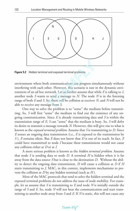
environment where both communications can progress simultaneously withoutinterfering with each other. However, this scenario is rare in the dynamic envi-ronment of an ad hoc network. Let us further assume that while E is talking to I,another node S wants to send a message to N. The node N is in the listeningrange of both E and S. So, there will be collision at receiver N, and N will not beable to receive any message from S.

One way to solve the problem is to “sense” the medium before transmit-ting. So, S will first “sense” the medium to find out the existence of any on-going communication. Since E is already transmitting data and S is within thetransmission range of E, S can “sense” that the medium is busy. So, S will deferits desire to transmit a message towards N. However, this will give rise to what isknown as the exposed terminal problem. Assume that S is transmitting to D. SinceE senses an ongoing data transmission (i.e., E is exposed to the transmission byS ), E remains silent. But E does not know that D is out of its reach. In fact, Ecould have transmitted to node I because these transmissions would not causeany collision either at D or at I.

A more serious problem is known as the hidden terminal problem. Assumethat node S is sending data to node D. A terminal H is hidden when it is faraway from the data source S but is close to the destination D. Without the abil-ity to detect the ongoing data transmission, H will cause a collision at D if Hstarts transmitting to J. MAC, in this context, implements mechanisms to pre-vent the collision at D by any hidden terminal (such as H ).

Most of the MAC protocols that tend to solve the hidden terminal and theexposed terminal problems do not address the issue of node mobility. For exam-ple, let us assume that S is transmitting to E and node N is initially outside therange of S and E. So, node N will not hear the communication and start trans-mitting to another node away from S and E. If N is static, this will not cause any


I E S D H J

N

Figure 5.2 Hidden terminal and exposed terminal problems.

TEAMFLY

Team-Fly®

interference. But let us assume that N is moving and coming closer to S and E,as shown in Figure 5.2. If N as a transmitter moves into the communicationrange of E, any transmission from N will collide with the ongoing communica-tion between S and E, and thus affect the channel throughput. This is called anintruding terminal problem.

The main purpose of MAC mechanisms in the context of ad hoc net-works is to ensure collision-free communication among nodes under differentconditions. These schemes, however, waste a large portion of the network capac-ity by reserving the wireless media over a large area. In other words, when S andD are communicating, a large number of nodes in the neighborhood of S and Dhave to sit idle, waiting for the data communication between S and D to fin-ish. To improve medium utilization, the use of directional antennas that canlargely reduce the radio interference, thereby improving the utilization of wire-less medium and consequently the network throughput, has been proposed. Forexample, when S and D are communicating with directional antennas at S andD directed towards each other, node E is free to communicate with anyone in itsneighborhood except S. Similarly, node H can communicate in all other direc-tion except towards D. However, in the context of ad hoc networks, it is difficultto find ways to control the direction of adaptive antennas for transmission andreception in each terminal in order to achieve an effective multihop communi-cation between any source and destination. This difficulty is mainly due tomobility and lack of centralized control in ad hoc networks. Thus, developing asuitable MAC protocol in ad hoc networks using adaptive antennas is a chal-lenging task.

Another way to improve medium utilization is to use mechanisms of con-trolling the transmission power of senders. For example, a sendermay reduce its current transmission range to a minimum value that is sufficientfor the successful reception of its message at the intended destination. Mediumutilization can be significantly increased because the severity of signal overlap-ping is reduced. However, adaptive power control mechanisms introduce addi-tional overhead and problems of route discovery and topology maintenance inad hoc networks. We will investigate these issues in the next chapter.

References


[2] Corson, M. S., and J. Macker, “Mobile Ad Hoc Networking (MANET): Routing Proto-col Performance Issues and Evaluation Considerations,’’ Request For Comments 2501,Internet Engineering Task Force, Jan. 1999.

Overview 123


[4] Johnson, B., and D. A. Maltz, “Dynamic Source Routing in Ad Hoc Wireless Networks,”T. Imielinski and H. Korth (eds.), Mobile Computing, Netherlands: Kluwer, 1996.

[5] Haas, Z. J., and S. Tabrizi, “On Some Challenges and Design Choices in Ad Hoc Com-munications,” IEEE MILCOM’98, Bedford, MA, Oct. 18–21, 1998.

[6] Lauer, G. S., “Packet-Radio Routing,” M. E. Steenstrup (ed.), Routing in CommunicationsNetworks, Englewood Cliffs, NJ: Prentice Hall, 1995, pp. 375–379.

[7] Baker, D. J., and A. Ephremides, “The Organization of a Mobile Radio Network Via aDistributed Algorithm,” IEEE Trans. Commun., Vol. COM-29, 1981.

[8] Gerla, M., and J. T. Tsai, “Multicluster, Mobile, Multimedia Radio Network,” ACMWireless Networks, Vol. 1, No. 3, 1995, pp. 255–265.

[9] Lin, R., and Mario Gerla, “Adaptive Clustering for Mobile Wireless Networks,” IEEEJournal on Selected Areas in Communications, Vol. 15, No. 7, Sept. 1997.

[10] Krishna, P., et al., “A Cluster-Based Approach for Routing in Ad Hoc Networks,” Proc. ofthe 2nd USENIX Symp. on Mobile and Location-Independent Computing, Apr. 1995.

[11] Perkins, E., and P. Bhagwat, “Highly Dynamic Destination-Sequenced Distance-VectorRouting (DSDV) for Mobile Computers,” ACM Comput. Commun. Rev., Vol. 24, No. 4,(ACM SIGCOMM’94) Oct. 1994, pp. 234–244.

[12] Perkins, C. E., and E. M. Royer, “Ad Hoc On-Demand Distance Vector Routing,” Proc.of the 2nd IEEE Workshop on Mobile Comp. Sys. And Apps., Feb. 1999, pp. 90–100.


6MAC Techniques in Ad Hoc Networks

6.1 MAC Protocols with Omnidirectional Antennas

When nodes in an ad hoc network use omnidirectional antennas, it isimplied that the transmitted signal from any node will spread equally wellin all directions within its transmission range. Similarly, as a receiver, anode will receive signals equally well from all directions. Traditionally, ad hocnetworks use omnidirectional antennas for their simplicity and lower cost.However, the use of directional antennas can largely reduce the radio interfer-ence, thereby improving the utilization of wireless medium and consequentlythe network throughput. So, researchers are also exploring the possibilities ofusing low-cost directional antennas in the context of ad hoc networks. In thissection, MAC protocols with omnidirectional antennas will be illustrated. In thenext section, MAC protocols with directional antennas will be discussed.

Designing an efficient and effective MAC protocol with collision avoid-ance capability in a mobile ad hoc network is a very challenging task because thenetwork is self-organizing without the aid of wired backbone or centralized net-work control. Some of the existing MAC protocols can be classified intoALOHA [1], Carrier Sense Medium Access (CSMA) [2], Busy Tone Multi-ple Access (BTMA) [3], Multiple Access with Collision Avoidance(MACA) [4], Media Access Protocol for Wireless LANs (MACAW) [5],Floor Acquisition Multiple Access (FAMA) [6], and Dual Busy Tone MultipleAccess (DBTMA) [7]. In ALOHA [1], each user can start a transmission at anytime without first sensing the channel status. The throughput is affected by fre-quent collisions. The slotted ALOHA protocol achieves a channel utilization of36% by dividing the channel into time slots. Transmission is allowed to start at

125

the beginning of a time slot only. Slotted ALOHA maintains a higher chan-nel utilization by avoiding collisions in the middle of the data transmis-sion, but it introduces somewhat of a longer access delay and morecomplexity due to the need for slot synchronization. CSMA protocols havebeen used in a number of packet-radio networks in the past [2]. In CSMA, eachuser senses the carrier before starting the transmission. The throughput is higherthan ALOHA because collisions may be avoided. However, the CSMA proto-cols do not address the hidden terminal problem and the exposed terminal prob-lem, as illustrated in Section 5.2.3.

The BTMA [3] was the first proposal to combat the hidden terminal prob-lems of CSMA. However, BTMA is designed for station-based net-works and requires dividing the channel into a message channel and the busytone channel. One of the first protocols for wireless networks based on a hand-shake between sender and receiver was the Split-Channel Reservation MultipleAccess (SRMA) [8]. It uses the Request-to-Send/Clear-to-Send (RTS/CTS) dia-log as a mechanism of handshaking. RTS/CTS dialog precedes the actual trans-mission of the data by the stations and allows the reserving of the channel, sothat collisions with other stations are avoided. The MACA [4] and MACAW [5]protocols use similar schemes in single channel networks. The protocols basedon an RTS/CTS-based handshaking mechanism can reduce the packet loss dueto hidden terminals. An explanation follows.

Let us refer to Figure 5.2. Before sending the data packets, S sends anRTS with proposed duration of data transmission to inform its neighbors aboutits willingness to start a communication with D. So, all the neighbors of S willbecome idle (neither transmit nor receive) during this period. If the intendeddestination D hears the RTS, D replies with CTS to inform its neighbors aboutits willingness to receive data from S. The neighbors of D that receives only CTScannot transmit (to avoid collision with D’s reception), but they can receivefrom other nodes outside the RTS/CTS boundaries. In some protocols, S issuesanother packet called a data-sending packet after it receives the CTS packet inorder to ensure its neighbors that a successful reservation has been accom-plished. This avoids unwanted waiting of nodes receiving only RTS under thecondition of unsuccessful negotiation between S and D. After data reception byD is over successfully, it issues an acknowledgement (ACK) to S. The ACKpacket at link level speeds up packet retransmission that is faster than relying onthe slow recovery at the transport layer.

Any other nodes overhearing the RTS must be close to node S and there-fore should remain silent for a time period long enough so that node S canreceive the returning CTS without any collision. Any other nodes overhearingthe CTS must be close to node D and therefore should refrain from transmis-sion for a time period that is long enough for the transmission of the proposeddata packet so that node D can receive the returning data packet without any


conflict. A hidden terminal (e.g., node H ), which is in the range of node D butout of the range of node S, will hear the CTS but not the RTS. It thereforeremains silent during the data transmission from node S to node D.

In the IEEE’s proposed standard for WLANs (IEEE 802.11) [9], itdescribes specifications on the parameters of both the physical (PHY) and MAClayers of the network. The PHY layer, which actually handles the transmissionof data between nodes, can use either direct sequence spread spectrum, fre-quency hopping spread spectrum, or infrared (IR) pulse position modulation.The initial specification of IEEE 802.11 makes provisions for data rates of either1 Mbps or 2 Mbps, and calls for operation in the 2.4- to 2.4835-GHz frequencyband, which is an unlicensed band for industrial, scientific, and medical (ISM)applications. The current version of IEEE 802.11b operates at 11 Mbps in the2.4 GHz band and communicates up to 150 feet. IEEE 802.11a operates at 40Mbps in the 5.8 GHz band. For IR transmission, it operates at 300 to 428,000GHz. Infrared transmissions require absolute LOS links (no transmission is pos-sible outside any simply connected space or around corners), as opposed to RFtransmissions, which can penetrate walls.

The basic medium access method for IEEE 802.11 relies on the Distrib-uted Coordination Function (DCF), which uses CSMA/Collision Avoidancewith RTS/CTS-data-ACK, as discussed before. A node willing to transmitsenses the medium first to determine if it is idle. If it is busy, the node waits untiltransmission stops and then enters into a random back-off procedure by settingan internal counter. This back-off counter determines the amount of time thenode must wait until it is allowed to transmit its packet. During periods whenthe channel is clear, the node willing to transmit decrements its back-off coun-ter. When the back-off counter reaches zero, the node starts transmitting pack-ets if the medium is still idle. Since the probability that two nodes will choosethe same back-off factor is small, this prevents multiple nodes from seizing themedium immediately after completion of the preceding transmission, and colli-sions between packets are minimized.

It is to be noted that CSMA/Collision Detection, which is commonlyused in wired LANs, is impractical in this context, because WLAN radios arehalf duplex and cannot receive while transmitting. Therefore, a collision cannotbe detected by a radio while transmission is in progress.

The basic RTS/CTS mechanism described above is supposed to preventall other nodes in the receiver’s range from transmitting. However, CTS packetscan still be destroyed by collisions. It has been shown [7] that the probability ofCTS packet collision in a multihop network that uses the basic RTS/CTS dia-logue rules can be as high as 60% when the network operates at high traffic load.To overcome this, the DBTMA scheme [7] is proposed. It is based on both theRTS/CTS dialogue and the carrier-sensing feature. In particular, the carriersensing is performed by the introduction of two busy tones, which indicate the

MAC Techniques in Ad Hoc Networks 127

status of the shared channel in a particular geographical area. This significantlyreduces the chances of destruction of the actual data packets due to transmissioncollisions, which further improves the scheme’s utilization. In this protocol, thesingle common channel is split into two subchannels: a data channel and a con-trol channel. Data packets are transmitted on the data channel, while controlpackets (RTS and CTS, for example) are transmitted on the control channel.Additionally, two busy tones are assigned to the control channel: the receivebusy tone, which shows that a node is receiving on the data channel; and thetransmit busy tone, which shows that a node is transmitting on the data chan-nel. The DBTMA scheme significantly improves the performance over the basicRTS/CTS-based schemes. However, the use of a separate channel just to conveythe state of the data channel may not be a desirable feature in the context of anad hoc wireless environment.

FAMA [6] is another proposal to improve basic RTS/CTS-based proto-col. FAMA permits a sender to acquire control of the channel in the vicinityof a receiver dynamically, before transmitting data packets. The floor acquisi-tion strategy uses an RTS/CTS handshake and is based on a few simple princi-ples: (1) making the senders listen to the channel before transmitting RTSs; (2)implementing a busy tone mechanism using a single channel and half-duplexradios by making the receiver send CTSs that last long enough for the hiddensenders to realize that they must back off; and (3) providing priority to those sta-tions who successfully complete a handshake. FAMA is the first single-channelprotocol to provide the equivalent functionality of a busy tone solution, and itsubstantially improves the performance by avoiding collisions.

MACA, MACAW, FAMA, and similar protocols depend on RTS/CTSdialogue to solve the hidden terminal and the exposed terminal problems. How-ever, they do not address the issue of node mobility. The fact that a mobile nodedid not hear a RTS/CTS dialog does not indicate that the channel is indeed freefor use. For example, if a node not hearing the RTS/CTS dialogue moves intothe communication range of a receiver, any transmission of the intruder will col-lide with the ongoing one, and thus affect the channel throughput. This is calledan intruding terminal problem [10]. In order to solve the intruding terminalproblem, different spread spectrum channels for control messages (i.e., RTS andCTS) and data messages to different nodes have been proposed in [10]. Thus,an ongoing data transmission is safeguarded against collisions due to the controlor data message from an intruder.

6.2 MAC Protocols with Directional Antennas

The RTS/CTS-based scheme using omnidirectional antennas wastes a large por-tion of the network capacity by reserving the wireless media over a large area.


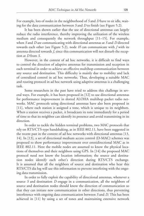
For example, lots of nodes in the neighborhood of S and D have to sit idle, wait-ing for the data communication between S and D to finish (see Figure 5.2).

It has been shown earlier that the use of directional antennas can largelyreduce the radio interference, thereby improving the utilization of the wirelessmedium and consequently the network throughput [11–15]. For example,when S and D are communicating with directional antennas at S and D directedtowards each other (see Figure 5.2), node H can communicate with J with itsantenna directed towards J, since this communication will not disturb the recep-tion at D from S.

However, in the context of ad hoc networks, it is difficult to find waysto control the direction of adaptive antennas for transmission and reception ineach terminal in order to achieve an effective multihop communication betweenany source and destination. This difficulty is mainly due to mobility and lackof centralized control in ad hoc networks. Thus, developing a suitable MACand routing protocol in ad hoc network using adaptive antennas is a challengingtask.

Some researchers in the past have tried to address this challenge in sev-eral ways. For example, it has been proposed in [12] to use directional antennasfor performance improvement in slotted ALOHA multihop packet radio net-works. MAC protocols using directional antennas have also been proposed in[11], where each station is assigned a tone, which is unique to its neighbors.When a station receives a packet, it broadcasts its tone immediately for a periodof time so that its neighbor can identify its presence and avoid transmitting in itsdirection.

In order to tackle the hidden terminal problems, two MAC protocols thatrely on RTS/CTS-type handshaking, as in IEEE 802.11, have been suggested inthe recent past in the context of ad hoc networks with directional antennas [13,14]. In [13], a set of directional medium access control (D-MAC) schemes wasproposed to show performance improvement over omnidirectional MAC as inIEEE 802.11. Here the mobile nodes are assumed to know the physical loca-tions of themselves and their neighbors using GPS. In [14] the proposed MACprotocol need not know the location information; the source and destina-tion nodes identify each other’s direction during RTS/CTS exchange.It is assumed that all the neighbors of source and destination who hear thisRTS/CTS dia log will use this information to prevent interfering with the ongo-ing data transmission.

In order to fully exploit the capability of directional antennas, whenever asource S and destination D engage in a communication, all the neighbors ofsource and destination nodes should know the direction of communication sothat they can initiate new communication in other directions, thus preventinginterference with ongoing data communication between S and D. This has beenachieved in [11] by using a set of tones and maintaining extensive network


status information at each node in the network. In [14] it is assumed that allnodes are able to maintain a unified and common coordinate system to markthe orientation of antennas with respect to each other at all times, irrespective oftheir movements. They suggest using some direction-finding instrument such asa compass in each node, and this requires additional hardware in each user ter-minal. Moreover, the probability of control packet collisions [13] has not beentaken into account in [14]. So, an appropriate null-steering mechanism needs tobe implemented to avoid control packet collisions and to increase the systemthroughput through overlapping communication.

An adaptive MAC protocol based on electronically steerable passive arrayradiator (ESPAR) antennas has been proposed [15] to overcome these difficul-ties. Each node keeps certain neighborhood information dynamically throughthe maintenance of an Angle–Signal-to-Interference-and-Noise Ratio (SINR)Table (AST), so that each node knows the direction of communication eventsgoing on in its neighborhood at that instant of time. Moreover, appropriatemechanisms for null steering of directional antennas in user terminals can helpexchange the neighborhood information in the presence of an ongoing commu-nication and can drastically improve the medium utilization through overlap-ping communications in different directions. The AST will also improve theperformance of directional routing, since it helps each node determine the bestpossible direction of communication with any of its neighbors.

In order to make the directional routing effective, a node should knowhow to effectively set its transmission direction to transmit a packet to its neigh-bors. So, each node periodically collects its neighborhood information andforms an AST. SINRu

n, m(t) is a number associated with each link l un m, , and is a

measurable indicator of the strength of radio connection from node n to m at anangle u with respect to n and as perceived by m at any point of time t. The ASTof node n specifies the strength of radio connection of its neighbors with respectto n at a particular direction.

Affinity of node m with respect to node n, awn, m(t), is a number associated

with a link l wn m, , at time t , such that aw

n, m(t) = Max [SINRun, m(t), 0<u <360].

In other words, the transmission angle w with respect to n maximizes thestrength of radio connection from n to m, as perceived by m at any point oftime. This maximum SINR value is the affinity of m with respect to n, and thisis obtainable when the antenna at n is directed towards m at an angle w withrespect to n. Based on this, a Neighborhood-Link-State Table (NLST) at eachnode is formed.

In this MAC protocol, initially, when node n wants to communicate withm, it sends omnidirectional RTS to inform all the neighbors of n, including m,that a communication from n to m has been requested. It also specifies theapproximate duration of communication between n and m. All the neighboringnodes of n keep track of this request from node n, whose direction is known to


each of them from the respective AST. The target node m sends omnidirectionalCTS to grant the request and to inform the neighbors of m that m is receivingdata from n. It also specifies the approximate duration of communication. Allthe neighboring nodes of m keep track of the receiving node m, whose directionis known to each of them from the respective AST.

On receiving CTS, node n issues omnidirectional start-of-data communi-cation (SDC) to inform that the data communication will start from n to m. If,after getting RTS, SDC is not received within a timeout, RTS is ignored. Thereceiver acknowledges completion of a successful data communication by send-ing an ACK to the transmitter.

Other nodes in the neighborhood of n and m can issue both RTS and CTSwithout disturbing the communication between n and m, which is illustratedbelow. Let us assume another pair of nodes X and Y, both in the neighborhoodof n and m, desires to communicate. Both of them have already receivedRTS/CTS from n and m. From their respective ASTs, both X and Y know thedirection of n and m. If the directional beam from X to Y captures n or m, thenthe node X has to sit idle and defer its desire. Otherwise, node X can issue anRTS. In other words, X can issue an RTS only if this communication does notinterfere with n or m. The RTS issued by X, however, will be selectively omnidi-rectional: X will issue the RTS avoiding interference with n and m. Similarly, Ywill respond to this RTS by sending a CTS if the directional beam from Y to Xdoes not captures n or m. The CTS issued by Y will also be selectively omnidi-rectional: Y will issue a CTS avoiding interference with n and m.

Some nodes around n and m will not receive RTS/CTS from X and Y andtherefore will be unaware of this communication event between X and Y. So,some of these nodes (including n or m, after the communication between n andm is over) may initiate another communication, which may disturb the commu-nication between X and Y. To avoid this, both of the antennas in X and Y willsteer their nulls in the directions towards n and m so that they will be unaffectedby the communication situation described above.

Any other nodes within the transmission beam of an ongoing communica-tion will sit idle during the communication process. But, each of them will bewaiting in omnidirectional receive mode with its null steer towards the directionof communication. This will enable the idle nodes to receive RTS/CTSexchange from nodes that are unaware of the communication process. This willhappen in the following scenario: When X and Y are communicating simultane-ously with n and m, some nodes around n and m will not receive RTS or CTS orboth from X and Y (as mentioned earlier). So, these nodes will be unaware ofthis communication between X and Y. So, some of these nodes may initiateanother communication. But, they will issue omnidirectional RTS/CTS, sincethey are unaware of any communication process. All nodes in the X-Y beam(excluding X and Y) need to receive this RTS/CTS to become aware of this new


communication. So, during the communication between X and Y, all othernodes in this region will steer their nulls towards X-Y and wait in the omnidirec-tional receive mode. Nodes X and Y, as mentioned earlier, will steer their nullsin the directions of n and m so that they will be unaffected by the probable com-munication in those regions. After the communication between X and Y is over,X and Y will collect this information from their neighbors during the next cycleof angle-SINR formation of X and Y.

This can be extended to ensure conflict-free multiple communicationsimultaneously. The number of simultaneous communications, however,depends on the null-steering capability and also on the current topology of thenetwork.

6.3 Discussions

Researchers are still working to address several performance concerns of MACprotocols proposed in the context of ad hoc networks [16]. One of the impor-tant issues is to ensure fairness in medium access. In a multihop configurationusing CSMA/CA-based MAC protocols with exponential back-off mechanism,all the nodes may not be able to access the shared medium equally well all of thetime. This results in severe performance degradation. The performance degradesfurther if we assume asymmetric links. Note that all of the above protocolsassume the presence of symmetric links. This is valid for a network in which allnodes transmit at the same power level. However, an ad hoc network may becomprised of devices that have different transmit power capabilities. In anyevent, it will be critical to ensure that the MAC protocol in use does not undulyfavor devices that can transmit at higher power levels [17].

Researches are also focusing on power-controlled MAC protocols thatwould improve channel utilization to a large extent [18, 19]. The basic ideabehind conventional CSMA/CA MAC protocol is to reserve the transmissionand reception areas of both source and destination. The goal of power-controlled MAC is that, a pair of communicating nodes adjusts their power levelto acquire the minimum area of the floor that is needed for it to successfullycomplete a data transmission [19]. Power-controlled multiple access is achievedby adhering to two key principles [19]:

1. The power conserving principle dictates that each station must trans-mit at the minimum power level that is required to be successfullyheard by its intended receiver.

2. The cooperation principle dictates that no station that commences anew transmission can transmit loud enough to disrupt ongoingtransmissions.


TEAMFLY

Team-Fly®

Enforcing these two principles can help achieve efficient power-controlledmultiple accesses within the framework of collision avoidance protocols.

References

[1] Abramson, N., “The ALOHA System – Another Alternative for Computer Communica-tions,” Proc. Fall Joint Comput. Conf., AFIPS Conf., 1970, pp. 281–285.

[2] Kleinrock, L., and F. A. Tobagi, “Packet Switching in Radio Channels: Part I—CarrierSense Multiple-Access Modes and Their Throughput-Delay Characteristics,” IEEE Trans.Commun., Vol. COM-23, No. 12, Dec. 1975, pp. 1400–1416.

[3] Tobagi, F. A., and L. Kleinrock, “Packet Switching in Radio Channels: Part II. The Hid-den Terminal Problem in Carrier Sense Multiple Access Modes and the Busytone Solu-tion,” IEEE Trans. on Commun., Vol. COM-23, No. 12, 1975, pp. 1417–1433.

[4] Karn, P., “MACA—A New Channel Access Method for Packet Radio,” ARRL/CRRLAmateur Radio 9th Computer Networking Conf., 1990, pp. 134–140.

[5] Bharghavan, V., et al., “MACAW: A Media Access Protocol for Wireless LAN’s,” ACMSIGCOMM’94, 1994, pp. 212–225.

[6] Fuller, L., and J. J. Garcia-Luna-Aceves, “Floor Acquisition Multiple Access (FAMA) forPacket-Radio Networks,” ACM SIGCOMM’95, 1995, pp. 262–273.

[7] Deng, J., and Z. J. Haas, “Dual Busy Tone Multiple Access (DBTMA): A MediumAccess Control for Multihop Networks,’’ Proc. of the IEEE Wireless Communications andNetworking Conf., New Orleans, LA, Sept. 1999.

[8] Tobagi, F. A., and L. Kleinrock, “Packet Switching in Radio Channels: Part III. Pollingand (Dynamic) Split-Channel Reservation Multiple Access Solution,” IEEE Trans. onCommun., Vol. COM-24, No. 8, 1976, pp. 832–845.

[9] Lough, Daniel L., T. Keith Blankenship, and Kevin J. Krizman, A Short Tutorial on Wire-less LANs and IEEE 802.11, The Bradley Department of Electrical and Computer Engineer-ing, Virginia Polytechnic Institute and State University, Blacksburg, VA, Apr. 2000.

[10] Ng, Mario Joa, “Routing Protocol and Medium Access Protocol for Mobile Ad Hoc Net-works,” Ph.D. Dissertation, Polytechnic University, Jan. 1999.

[11] Yum, T. S., and K. W. Hung, “Design Algorithms for Multihop Packet Radio Networkswith Multiple Directional Antennas Stations,’’ IEEE Trans. on Commun., Vol. 40, No. 11,1992, pp. 1716–1724.

[12] Zander, J., “Slotted ALOHA Multihop Packet Radio Networks with Directional Anten-nas,” Electronics Letters, Vol. 26, No. 25, 1990.

[13] Ko, Y. B., V. Shankarkumar, and N. H. Vaidya, “Medium Access Control ProtocolsUsing Directional Antennas in Ad Hoc Networks,’’ Proc. of IEEE INFOCOM 2000,March 2000.

[14] Nasipuri, A., et al., “A MAC Protocol for Mobile Ad Hoc Networks Using DirectionalAntennas,” Proc. of the IEEE WCNC 2000, 2000.


[15] Bandyopadhyay, S., et al., “An Adaptive MAC Protocol for Wireless Ad Hoc CommunityNetwork (WACNet) Using Electronically Steerable Passive Array Radiator Antenna,”GLOBECOM 2001, San Antonio, TX, Nov. 2001.

[16] Xu, S., and T. Saadawi, “Does the IEEE 802.11 MAC Protocol Work Well in MultihopWireless Ad Hoc Networks?” IEEE Communication Magazine, June 2001, pp. 130–137.

[17] Poojary, N., S. V. Krishnamurthy, and S. Dao, “Medium Access Control in a Network ofAd Hoc Nodes with Heterogeneous Transmit Power Capabilities,” Proceedings of ICC2001, Helisinki, 2001.

[18] Wu, Shih-Lin, and Yu-Chee Tseng, “Intelligent Medium Access for Mobile Ad Hoc Net-works with Busy Tones and Power Control,” JSAC, Vol. 18, No. 9, Sept. 2000.

[19] Monks, Jeffrey P., Vaduvur Bharghavan, and Wen-mei Hwu, “A Power-Controlled Mul-tiple Access Protocol for Wireless Packet Networks,” IEEE INFOCOM 2001, Anchorage,Alaska, Apr. 2001.


7Routing Protocols in Ad Hoc WirelessNetworks

In this chapter, we will discuss various routing protocols proposed so far in thecontext of ad hoc networks. Both unicast and multicast routing protocols will beexamined and the performance of some of the major unicast and multicast rout-ing protocols will be illustrated.

7.1 Introduction

The problem of routing in a network has two components: route discovery androute maintenance. In order to communicate with a destination, a source needsto discover a suitable route for sending packets to that destination. However, asthe status of different links (or routers) used in this route change, changes in theroute may be necessary and a new route may need to be discovered. Conven-tional routing protocols for wired networks commonly use either distance vectoror link-state protocols [1]. These protocols integrate route discovery with routemaintenance by sending routing update packets. If the status of a link or routerchanges, the update packets will eventually reflect the changes to all other rout-ers. As a result, new routes may be computed, if needed. These protocols can betermed proactive protocols because they attempt to discover and maintain routescontinuously so that routes are known a priori when needed.

In distance vector routing (DVR) protocols, each router periodically broad-casts to its neighbors its view of the distance to all other routers, and each routercomputes the shortest path to every other router based on the advertised infor-mation. By comparing the distances received for each destination from each of

135

its neighbors, a router can determine which of its neighbors is the correct “nexthop” on the shortest path toward each destination. When a source wants to senda data packet to a destination, the source simply forwards the data packet to thecorrect next-hop router. This router, in turn, forwards the packet to the correctnext hop. This will continue till the packet reaches its destination. DVR suffersfrom slow convergence and loop formation. These loops are formed becauseeach router chooses its next hops in a distributed fashion based on possibly oldand invalid information. Furthermore, routing updates may have to be propa-gated to a large number of routers. Examples of DVR protocols include therouting protocol used in the DARPA Packet Radio Network [2] and the originalrouting protocol for the ARPANET [3].

In link-state routing (LSR) protocols, each router maintains its view of theentire network topology. To maintain this, each router periodically broadcasts alink-state packet (LSP) containing a list of its neighbors and the cost of each linkto its neighbors. This information from each router eventually reaches all otherrouters in the network in a periodic fashion. Given this information about thecost of links in the network, each router can compute the best path to each pos-sible destination. When a source wants to send a data packet to a destination,the source computes the best path to the destination and then forwards the datapacket to the correct next hop router based on this computed best path. Thisrouter, in turn, computes the best path towards the destination and forwards thepacket to the correct next hop. This will continue until the packet reaches itsdestination. LSR protocols converge much more quickly when conditions in thenetwork change. However, it generally requires more computation time thanthat taken by the distance vector algorithm because each router computes thecomplete shortest path to each possible destination. It also consumes more net-work bandwidth than the distance vector algorithm because the routing updatesfrom each router are broadcast to all other routers in the entire network. Exam-ples of LSR protocols include the “new” routing protocol that replaced the origi-nal protocol for the ARPANET [3] and open shortest path first (OSPF) [4].

A natural method for trying to provide routing in an ad hoc network is tosimply treat each mobile host as a router and to run a conventional routing pro-tocol between them [2]. However, use of these conventional routing protocolsin an ad hoc network, treating each mobile host as a router, gives rise to a seriesof problems, as illustrated in [5, 6]:

• Transmission between two hosts over a wireless network does not nec-essarily work equally well in both directions. Thus, some routes deter-mined by conventional routing protocols may not work in someenvironments.

• Wired networks are usually explicitly configured to have only a smallnumber of routers connecting any two networks. In the ad hoc wireless


environment, each node is a router and too many paths exist betweenany two nodes in the network. These redundant paths unnecessarilyincrease the size of routing updates that must be sent over the networkand increase the computational as well as communication overhead.

• Periodic broadcasting of routing updates wastes network bandwidth inad hoc wireless environments. Routing updates from mobile hosts out-side each other’s transmission range will not interfere with each other,but where many mobile hosts are within transmission range of eachother, their routing updates will consume each other’s networkbandwidth.

• In a highly dynamic ad hoc network, the rate of topology change maybe higher than the rate of route requests. In such an environment, peri-odic updates could be a waste because most of this routing updateinformation is never used.

• Most mobile hosts in an ad hoc network will be operating on a limitedbattery power, and periodically sending routing updates wastes batterypower.

So we find that the conventional, proactive routing protocols place tooheavy a computation and communication demand on each mobile host in mul-tihop wireless networks. Additionally, convergence characteristics of these pro-tocols are not good enough for ad hoc networks [6]. The speed of convergencemay be improved by sending routing updates more frequently, but this willwaste more bandwidth and battery power. Moreover, this may be a wastefuleffort altogether when topology changes are less frequent. Keeping these factorsin mind, several researchers have proposed modifications of these conventionalprotocols to suit the environment of ad hoc wireless networks. For example,researchers have focused on restricting the propagation of routing updates,thereby reducing the control overheads [7]. At the same time, a lot of work hasbeen done in designing and developing alternative demand-driven routing pro-tocols [8], termed reactive protocols. These protocols are based on separate routediscovery and route maintenance protocols and do not require periodic routeupdates; they invoke route determination procedure only on demand. When-ever a source node requires a route to a destination, it initiates a route-discoveryprocess within the network. The source node broadcasts a route-request packetto its neighbors, which in turn forward the request to their neighbors, and so on,until the destination is located. The destination then responds by sending aroute-reply packet back to the source node through the intermediate nodes.Once a route has been established, it is maintained by a route-maintenance pro-cedure until either the destination becomes inaccessible from the source, or theroute is no longer desired.

Routing Protocols in Ad Hoc Wireless Networks 137

The performance of the above approach depends on two major factors: (1)how frequently a route discovery is needed, and (2) how often route mainte-nance is needed. If the communication requirement is high, frequent route dis-covery would be needed. Since each route discovery is associated with floodingof route-request packets throughout the network, multiple route discoveries at atime will flood the network with route-request packets, increasing congestionand collision in the network. At the same time, if the nodes are mobile, requir-ing frequent route maintenance, this would in turn increase the control packetsin the network further. In the reactive mechanism, computation and communi-cation overhead are reduced only when the demand for communication is less.Moreover, this reduced computation and communication overhead is achievedat the expense of a longer delay in route-setup procedure. Performance can beimproved through aggressive route caching and full use of information in thecache [6]. However, additional effort would be needed to detect the staleness ofthe information in the cache. Another way to decrease control packets is direc-tional propagation of route-request packets. All of these issues will be discussedin detail in Section 7.2.2.

7.2 Unicast Routing Protocols in Ad Hoc Networks

7.2.1 Proactive Routing Protocols

7.2.1.1 Destination-Sequenced Distance Vector Routing Protocol (DSDV)

In DSDV [9], each node maintains a routing table, which has an entry for eachdestination in the network. The attributes for each destination are the next hop,metric (hop counts), and a sequence number originated by the destination node.To maintain the consistency of the routing tables, DSDV uses both periodicand triggered routing updates; triggered routing updates are used in addition tothe periodic updates in order to propagate the routing information as quickly aspossible when there is any topological change. The update packets include thedestinations accessible from each node and the number of hops required toreach each destination along with the sequence number associated with eachroute.

Upon receiving a route-update packet, each node compares it to the exist-ing information regarding the route. Routes with old sequence numbers are sim-ply discarded. In case of routes with equal sequence numbers, the advertisedroute replaces the old one if it has a better metric. The metric is then incre-mented by one hop since incoming packets will require one more hop to reachthe destination. A newly recorded route is immediately advertised to itsneighbors.


When a link to the next hop is broken, any route through that next hop isimmediately assigned an infinity metric and assigned an updated sequencenumber. This is the only case when sequence numbers are not assigned by thedestination. When a node receives an infinity metric and it has an equal or latersequence number with a finite metric, a route update broadcast is triggered.Therefore, routes with infinity metrics will be quickly replaced by real routespropagated from the newly located destination.

One of the major advantages of DSDV is that it provides loop-free routesat all instants. It has a number of drawbacks however. Optimal values for theparameters, such as maximum settling time, for a particular destination are diffi-cult to determine. This might lead to route fluctuations and spurious advertise-ments resulting in waste of bandwidth. DSDV also uses both periodic andtriggered routing updates, which could cause excessive communication over-head. In addition, in DSDV, a node has to wait until it receives the next routeupdate originated by the destination before it can update its routing table entryfor that destination. Furthermore, DSDV does not support multipath routing.

7.2.1.2 Wireless Routing Protocol (WRP)

WRP [10] is also based on distance vector algorithm. To avoid the loopingproblem present in the distance vector algorithm, WRP includes second-to-lasthop (predecessor) information for each destination. This predecessor informa-tion is included in two tables kept at each node: a distance table and a routingtable. The distance table of node i is a matrix containing, for each destination jand each neighbor k, the distance to j and the predecessor when k is chosen asthe next hop to reach j. The routing table contains an entry for each destination,and the attributes for each destination include the next hop, distance, and thepredecessor.

To keep a consistent view of the network and to respond to topologicalchanges, each node exchanges update packets with its neighbors. An updateentry specifies a destination, a distance to the destination, and a predecessor tothe destination. Upon receiving an update packet, each node updates the dis-tance and the predecessor entries in the distance table. Let’s say a node i receivesan update from its neighbor k regarding destination j. In addition to updatingthe distance and the predecessor information for the destination j and neighbork pair, WRP determines if the path to destination j through any other neighborsincludes node k and updates affected entries. Note that by back-tracing thepredecessor information kept in the distance table, the complete path can befound. After updating the distance table, each node also updates its routing tableaccordingly by choosing the neighbor that offers the smallest cost to the givendestination as the next hop to reach that destination.

The major advantage of WRP is that it reduces temporary looping byusing the predecessor information to identify the route. This in turn reduces the


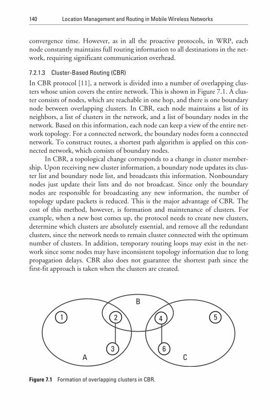
convergence time. However, as in all the proactive protocols, in WRP, eachnode constantly maintains full routing information to all destinations in the net-work, requiring significant communication overhead.

7.2.1.3 Cluster-Based Routing (CBR)

In CBR protocol [11], a network is divided into a number of overlapping clus-ters whose union covers the entire network. This is shown in Figure 7.1. A clus-ter consists of nodes, which are reachable in one hop, and there is one boundarynode between overlapping clusters. In CBR, each node maintains a list of itsneighbors, a list of clusters in the network, and a list of boundary nodes in thenetwork. Based on this information, each node can keep a view of the entire net-work topology. For a connected network, the boundary nodes form a connectednetwork. To construct routes, a shortest path algorithm is applied on this con-nected network, which consists of boundary nodes.

In CBR, a topological change corresponds to a change in cluster member-ship. Upon receiving new cluster information, a boundary node updates its clus-ter list and boundary node list, and broadcasts this information. Nonboundarynodes just update their lists and do not broadcast. Since only the boundarynodes are responsible for broadcasting any new information, the number oftopology update packets is reduced. This is the major advantage of CBR. Thecost of this method, however, is formation and maintenance of clusters. Forexample, when a new host comes up, the protocol needs to create new clusters,determine which clusters are absolutely essential, and remove all the redundantclusters, since the network needs to remain cluster connected with the optimumnumber of clusters. In addition, temporary routing loops may exist in the net-work since some nodes may have inconsistent topology information due to longpropagation delays. CBR also does not guarantee the shortest path since thefirst-fit approach is taken when the clusters are created.


A C

B

1 2

3

4 5

6

Figure 7.1 Formation of overlapping clusters in CBR.

7.2.1.4 Cluster Head-Gateway Switch Routing (CGSR)

CGSR protocol [12] is also based on a cluster-based network architecture. InCGSR, specific nodes are designated to be cluster heads, which control channelaccess within a cluster at MAC layer. At MAC layer, cluster heads are given apriority, and thus they have more chances to transmit than other nodes. Allnodes within a cluster can communicate with its cluster head and possibly witheach other. To prevent frequent cluster head changes, the Least Cluster HeadChange Algorithm (LLC) is used.

In CGSR, the DSDV protocol is modified so that it can take an advantageof the clustering architecture. Specifically, hierarchical routing is used to routepackets. Each node maintains two tables: a cluster member table which maps thedestination node address to its cluster head address, and a routing table whichshows the next hop to reach the destination cluster. Both tables containsequence numbers to purge stale routes and prevent looping. In CGSR, packetsare routed alternatively through cluster heads and gateways. In other words, thetypical route looks like C1G1C2G2...CIGI, where Ci is a cluster head and Gi is agateway. This is shown in Figure 5.1 in Chapter 5. A gateway refers to a nodethat belongs to more than one cluster. Therefore, in CGSR, gateway-to-gatewayshortcuts are avoided. Even though this strict alternate routing results inincreased path length, this drawback is outweighed by its merits. Specifically,the presence of a cluster head between two gateways is advantageous since clus-ter heads have more chances to transmit than other nodes and a direct gateway-to-gateway communication requires that both gateways meet on the same codefor transmission, which can lead to code scheduling overhead and hence delay.

The major advantage of CGSR is that only the routes to the cluster headsare maintained due to the hierarchical routing. However, there is overhead asso-ciated with maintaining clusters. Specifically, each node needs to periodicallybroadcast its cluster member table and update its table based on the receivedupdates.

7.2.1.5 Fisheye State Routing

Fisheye State Routing (FSR) [7] introduces the notion of multilevel fisheyescope to reduce routing update overhead in large networks. Nodes exchangelink-state entries with their neighbors with a frequency that depends on distanceto destination. From link-state entries, nodes construct the topology map of theentire network and compute optimal routes. FSR uses the “fisheye” techniqueproposed by Kleinrock and Stevens [13], where the technique was used toreduce the size of information required to represent graphical data. The eye of afish captures with high detail the pixels near the focal point. The detail decreasesas the distance from the focal point increases. In routing, the fisheye approachtranslates to maintaining accurate distance and path quality information about


the immediate neighborhood of a node, with progressively less detail as the dis-tance increases. FSR is functionally similar to LS Routing in that it maintains atopology map at each node. The key difference is the way in which routinginformation is disseminated. In LS, link-state packets are generated and floodedinto the network whenever a node detects a topology change.

In FSR, link-state packets are not flooded. Instead, nodes maintain a link-state table based on the up-to-date information received from neighboringnodes, and periodically exchange it with their local neighbors only (no flood-ing). Through this exchange process, the table entries with larger sequence num-bers replace the ones with smaller sequence numbers. The FSR periodic tableexchange resembles the vector exchange in DSDV [9] where the distances areupdated according to the time stamp or sequence number assigned by the nodeoriginating the update. However, in FSR link states rather than distance vectorsare propagated. Moreover, like in LS, a full topology map is kept at each nodeand shortest paths are computed using this map.

In order to reduce the size of update messages without seriously affectingrouting accuracy, FSR uses the notion of multilevel fisheye scope. The scope isdefined as the set of nodes that can be reached within a given number of hops.The reduction of routing update overhead is obtained by using differentexchange periods for different entries in routing table. More precisely, entriescorresponding to nodes within the smaller scope are propagated to the neigh-bors with the highest frequency. The rest of the entries are sent out at a lowerfrequency. As a result, a considerable fraction of link-state entries are suppressedin a typical update, thus reducing the message size. This strategy producestimely updates from near stations, but creates large latencies from stations afar.However the imprecise knowledge of the best path to a distant destination iscompensated by the fact that the route becomes progressively more accurate asthe packet gets closer to destination. As the network size grows large, a “graded”frequency update plan must be used across multiple scopes to keep the overheadlow.

7.2.2 Reactive Routing Protocols

7.2.2.1 Dynamic Source Routing (DSR)

Dynamic source routing [14] is based on source routing, where the source speci-fies the complete path to the destination in the packet header and each nodealong this path simply forwards the packet to the next hop indicated in the path.It utilizes a route cache where routes it has learned so far are cached. Therefore, asource first checks its route cache to determine the route to the destination. If aroute is found, the source uses this route. Otherwise, the source uses a route dis-covery protocol to discover a route.


TEAMFLY

Team-Fly®

In route discovery, the source floods a query packet through the ad hocnetwork, and the reply is returned by either the destination or another host,which can complete the query from its route cache. Each query packet has aunique ID and an initially empty list. When receiving a query packet, if a nodehas already seen this ID (i.e., duplicate) or it finds its own address alreadyrecorded in the list, it discards the copy and stops flooding; otherwise, itappends its own address in the list and broadcasts the query to its neighbors. If anode can complete the query from its route cache, it may send a reply packet tothe source without propagating the query packet further. Furthermore, anynode participating in route discovery can learn routes from passing data packetsand gather this routing information into its route cache.

A route failure can be detected by the link-level protocol (i.e., hop-by-hopacknowledgments), or it may be inferred when no broadcasts have been receivedfor a while from a former neighbor. When a route failure is detected, the nodedetecting the failure sends an error packet to the source, which then uses routediscovery protocol again to discover a new route. Note that in DSR, no periodiccontrol messages are used for route maintenance.

The major advantage of DSR is that there is little or no routing overheadwhen a single or few sources communicate with infrequently accessed destina-tions. In such situation, it does not make sense to maintain routes from allsources to such destinations. Furthermore, since communication is assumed tobe infrequent, a lot of topological changes may occur without triggering newroute discoveries.

Even though DSR is suitable for the environment where only a few sourcecommunicate with infrequently accessed destinations, it may result in largedelay and large communication overhead in highly dynamic environment withfrequent communication requirement [15]. Furthermore, DSR may have scal-ability problem [16]. As the network becomes larger, control packets and mes-sage packets also become larger since they need to carry addresses for every nodesin the path. This may be a problem since ad hoc networks have limited availablebandwidth.

7.2.2.2 Ad Hoc On-Demand Distance Vector Routing (AODV)

The Ad Hoc On-Demand Distance Vector (AODV) [17, 18] routing protocolshares DSR’s on-demand characteristics in that it also discovers routes on an “asneeded’’ basis via a similar route discovery process. However, AODV adopts avery different mechanism to maintain routing information. It uses traditionalrouting tables, one entry per destination. This is a departure from DSR, whichcan maintain multiple route cache entries for each destination. Without sourcerouting, AODV relies on routing table entries to propagate a route reply back tothe source and, subsequently, to route data packets to the destination. AODVuses sequence numbers maintained at each destination to determine freshness of


routing information and to prevent routing loops. These sequence numbers arecarried by all routing packets.

When a route is needed, a node broadcasts a route request message. Theresponse message is then echoed back once the request message reaches the desti-nation or an intermediate node that contains a fresh route to the destination.For each route, a node also maintains a list of those neighbors actively using theroute. A link breakage causes immediate link failure notifications to be sent tothe affected neighbors. Similar to DSDV, each route table entry is tagged with adestination sequence number to avoid loop formation. Moreover, nodes are notrequired to maintain routes that are not active. Thus, wireless resource can beeffectively utilized. However, since flooding is used for route search, communi-cation overhead for route search is not scalable for large networks. As routemaintenance considers only the link breakage and ignores the link creation, theroute may become nonoptimal when network topology changes. Subsequentglobal route search is needed when the route is broken.

An important feature of AODV is maintenance of timer-based states ineach node, regarding utilization of individual routing table entries. A routingtable entry is “expired” if not used recently. A set of predecessor nodes is main-tained for each routing table entry, indicating the set of neighboring nodes thatuse that entry to route data packets. These nodes are notified with route errorpackets when the next hop link breaks. Each predecessor node, in turn, forwardsthe route error to its own set of predecessors, thus effectively erasing all routesusing the broken link.

The recent specification of AODV [19] includes an optimization tech-nique to control the route request flood in the route discovery process. It uses anexpanding ring search initially to discover routes to an unknown destination. Inthe expanding ring search, increasingly larger neighborhoods are searched tofind the destination. The search is controlled by the TTL field in the IP headerof the route request packets. If the route to a previously known destination isneeded, the prior hopwise distance is used to optimize the search.

7.2.2.3 Temporally Ordered Routing Algorithm

Temporally Ordered Routing Algorithm (TORA) [16] is a highly adaptiveloop-free distributed routing protocol for multihop networks. A key concept inthe protocol’s design is an attempt to decouple the generation of far-reachingcontrol message propagation from the dynamics of the network topology. Thebasic, underlying algorithm is one of a family of algorithms referred to as linkreversal algorithms. In particular, the protocol’s reaction to certain link failures isstructured as a temporally ordered sequence of diffusing computations, eachcomputation consisting of a sequence of directed link reversals.

TORA is partly based on the classical work by Gafni and Bertsekas [20] inorder to maintain a destination-oriented directed acyclic graph (DAG) in the


face of topology changes. A DAG is considered destination oriented, if for everynode there is a path to a given destination. If this configuration is lost due tolink failures, a series of link reversals take place to ensure that the graph againbecomes destination-oriented in finite time. Based on the query/reply processproposed in [21], a sequence of directed links leading from the source to the des-tination is formed (route discovery and construction phase) in a source-initiatedfashion. From that point it is maintained (route maintenance phase) using linkreversal, whenever topology change causes a node to loose its last downstreamlink. If the destination becomes unreachable because of a network partition, theprotocol erases (route eraser phase) all invalid routes.

TORA provides multiple paths to a destination and ensures they areloop-free. This is a destination-oriented protocol in which logically separate ver-sion of the protocol is run for each destination in active communication. How-ever, after the DAG creation, new links would not be considered unless theDAG becomes disconnected. Therefore, the route may become nonoptimal. Inaddition, communication overhead for route creation is not scalable becauseflooding is used. TORA does not guarantee generation of shortest path routes.Another drawback of TORA is that it may take long time for the protocol toconverge if a link failure partitions the network.

7.2.2.4 Associativity-Based Routing (ABR)

Associativity-based routing [22] also uses a source-initiated method, that is,ABR only maintains routes for sources that actually desire routes. To find aroute to the desired destination, ABR also uses query-reply control packets. Asin TORA and DSR, the source floods a query packet through the ad hoc net-work to discover a route. However, unlike in TORA and DSR, the best route isselected by the destination based on the stability of the route and shortest path.A route is considered to be stable if it consists of nodes that have been stationaryfor a threshold period. The stationary period is measured in terms of associativ-ity ticks, which are described below.

Each node maintains multiple associativity ticks (one per each neighbor),which are initially set to zero. Periodically, each node broadcasts beacons identi-fying itself. Note that these beacons are not newly defined messages, but arelink-level messages, which are normally exchanged between nodes to maintainconnectivity. Therefore, no extra overhead is added. Each time a beacon isreceived, a node increments the associativity tick which is associated with thenode from which a beacon is received. If a neighboring node moves out of prox-imity, the associativity tick, which is associated with that neighbor is reset tozero. Therefore, if a mobile host has low associativity ticks with its neighbors, itindicates that the mobile host is in high state of mobility. On the other hand, ifa mobile host has high associativity ticks with its neighbors, it indicates that themobile host is in the stable (or stationary) state.


In route discovery, the source floods a query packet. As in DSR, a querypacket contains an initially empty list, and when receiving a query packet, anode appends its own address in the list. In ABR, however, a query packet alsocontains the associativity ticks along with other metrics such as hop count.When a node receives a query packet, it appends its address in the list, and it alsoappends the associativity ticks with its neighbors along with other metrics. Thenext succeeding node keeps only its upstream neighbor’s associativity tick,which is associated with it and erases all others. Therefore, when the querypacket reaches the destination, it will contain only the intermediate nodes’addresses and the associativity ticks for that path, together with routing infor-mation such as hop count.

After some time period, the destination will know all the possible routesand their qualities. It then selects the best route based on the selection criteria.The most important criterion in selecting a route is the stability of the routeindicated by the associativity ticks. Therefore, the destination chooses the routethat consists of nodes having high associativity ticks. If more than one route hasthe same degree of stability, the destination selects the shortest route. The desti-nation then sends a reply packet back to the source. Only the best route selectedwill be valid, while all other routes will be inactive. When a node moves, unlessit is the source, its immediate upstream node erases its route and tries to find analternate route using the localized query, thereby retaining the control packetslocally. Only when necessary, the full query-reply process is performed. Sourcemovement always invokes the full query-reply process.

The major advantage of ABR is that routes selected tend to be long-livedsince nodes that have been stationary for some time are less likely to move. Thisresults in fewer route reconstructions, thereby reducing the communicationoverhead. A possible drawback of ABR is that ABR may have scalability problemdue to the limited available bandwidth, since control packets and message pack-ets need to carry addresses for every nodes in the path as in DSR.

7.2.2.5 Signal Stability-Based Adaptive Routing (SSAR)

SSAR [23] also discovers a route only when desired by a source. To find a routeto the desired destination, SSAR also uses a query-reply process; the sourcefloods a query packet, and the destination determines the best route and returnsa reply packet to the source. The novelty of the SSAR protocol is the use of sig-nal strength as a route-selection criteria. The basic idea of SSAR is to select theroute that consists of links with the strong signals since such routes lead tolonger-lived routes due to the “buffer zone” effect and consequently require lessroute maintenance. The buffer zone effect is as follows: if a link between twonodes is a strong link (i.e., a link with strong signal strength), it will have tobecome a weak link before triggering a route reconstruction. In other words,


two nodes that make up the strong link can roam within a certain vicinity ofeach other without triggering a route reconstruction.

To take the signal strength into account in routing process, each nodeperiodically broadcasts link-level beacons identifying itself, and upon receiving abeacon, each node records the signal strength at which the beacon was received.If the signal strength is above the threshold, the link is marked as a strong link.Otherwise, it is marked as a weak link. When a node receives a query packet, itpropagates the query packet further only if the query packet is received over astrong link and the node has not seen this query packet before. A query packetthat is received over a weak link is dropped. When a query packet reaches thedestination, it contains the address of each intermediate node. The destinationselects the route recorded in the first received query packet since it is probablythe shortest path. It then sends a reply packet back to the source along theselected route.

Since only the query packets that are received over the strong links are for-warded further, a query packet may never reach the destination if there is noroute which consists of strong links. In this case, the source will not receive anyreply packet within some timeout period. When the timeout period expires, thesource can wait and try again later, or it may wish to find any route by speciallymarking the query packet. When a route failure is detected, the node detectingthe failure sends an error packet to the source, which then sends a message toerase the invalid route and uses route discovery protocol again to find a newroute.

The major advantage of SSAR is that routes selected tend to be long-lived,and this in turn reduces the number of route reconstructions required. Further-more, SSAR results in low packet loss since strong links are less vulnerable tointerference than weak links. A possible drawback of SSAR is that SSAR resultsin routes with slightly higher hop counts than optimal routing since SSAR pre-fers routes with strong links, which are likely to be between two hosts close toeach other.

7.2.2.6 Stability-Based Routing

In an ad hoc network, relationship among nodes is based on providing somekind of service, and stability can be defined as the minimal interruption in thatservice. Irrespective of the routing schemes, frequent interruption in a selectedroute would degrade the performance in terms of quality of service. Therefore,an important issue is to minimize route maintenance by selecting stable routes,rather than shortest route. The notion of stability of a path is dynamic andcontext-sensitive. Stability of a path is the span of life of that path at a giveninstant of time and it has to be evaluated in the context of providing a service. Apath between a source and destination is said to be stable if its span of life is suf-ficient to complete a required volume of data transfer from source to


destination. Hence, a given path may be sufficiently stable to transfer a smallvolume of data between source and destination; but the same path may beunstable in a context where a large volume of data needs to be transferred.

In stability based routing [24], a notion of link stability and path stabilityand their evaluation mechanism in the context of dynamic topology changes inan ad hoc network has been proposed. Subsequently, a distributed routingscheme among mobile hosts is proposed in order to find a path between themthat is stable in a specific context.

The strength of relationship between two nodes over a period of time isdefined as node-affinity or affinity. Informally speaking, link-affinity anm(t), asso-ciated with a link lnm at time t, is a prediction about the span of life of the link lnm

in a particular context. Link-affinity anm(t) at that instant of time is a function ofthe current distance between n and m, relative mobility of m with respect to n,and the transmission range of n. If transmission range of n and m are different,anm(t) may not be equal to amn(t). The node-affinity or affinity ηnm t( ) betweentwo nodes and its neighbor m is defined as min[anm(t), amn(t)]. The stability ofconnectivity between n and its neighbor m depends on ηnm . The unit of affinityis seconds.

To find out the link-affinity anm(t) at any instant of time, node n sends aperiodic beacon and node m samples the strength of signals received from noden periodically. Since the signal strength of n as perceived by m is a function f (Rn,dnm) where Rn is the transmission range of n, and dnm is the current distancebetween n and m at time t, the node m can predict the current distance dnm attime t between n and m. If M is the average velocity of the nodes, the worst-caselink-affinity anm(t) at time t is (Rn – dnm)/M, assuming that at time t, the node mhas started moving outwards with an average velocity M. For example, If thetransmission range of n is 300m, the average velocity is 10 m/s and current dis-tance between n and m is 100m, the life span of link lnm (worst case) is 20s,assuming that the node m is moving away from n in a direction obtained byjoining n and m.

The above method is simple, but is based on an optimistic assumptionthat node-distance can be deduced from signal strength. In real life, even if thetransceivers have the same transmission range, it will vary because of the differ-ences in battery power in each of them. Therefore, it may be difficult for onenode to estimate distance from another node by monitoring the current signalstrength only. So, a node m needs to monitor the change in signal strength of nover time to estimate link-affinity, as described below.

Let ∆Snm(t) be the change of signal strength at time t and is defined as:∆Snm(t) = Snm(t) – Snm(t – ∆t), where Snm(t) is the current sample value of

the signal strength of node n as perceived by node m at time t, Snm(t – ∆t) is theprevious sample value at time (t – ∆t) and ∆t is the sampling interval. Let S′nm(t)be the rate of change of signal strength at time t and is defined as S′nm(t) =


(∆Snm(t) / ∆t ) and let S′nm(t)avg is the average rate of change of signal strength attime t over the past few samples. Let St be the threshold-signal strength: whenthe signal strength Snm associated with lnm goes below St, we assume that the linklnm is disconnected. Further, we define

anm (t) = high, if S′nm(t)avg is positive;= (St – Snm(t) ) / S′nm(t)avg, if S′nm(t)avg is negative.

If ∆Snm(avg) is positive, it indicates that the link-affinity is increasing and thetwo nodes are coming closer. Hence, link-affinity is termed high at that instantof time.The value for high is computed as (transmission range / average nodevelocity) and is approximately equal to the time taken by a node m to cross theaverage transmission range of node n with an average velocity. However, as indi-cated earlier, even if S′nm(t)avg is positive, a node p N n∈ in the periphery of thetransmission range of n is weakly connected to n compared to a node p N n∈which is closer to n. Thus, the chance of m going out of the transmission rangeof n due to a sudden outward mobility of either m or n is more than that of p.Thus, if S′nm(t)avg is positive, a correction factor µ is used to moderate this highvalue. This correction factor µ is equal to (1 – St / Snm(t)) and aVnm(t) = µ* high, ifS′nm(t)avg is positive. This indicates that if Snm(t) is very close to S t , µ will be closeto zero and consequently anm(t) will also become close to zero, even if S(nm(t)!AVG

is positive.As indicated earlier, the node-affinity or affinity between two nodes n and

m, ηnm(t), is defined as min[anm(t) , amn(t)].Given any path p = (i, j, k,..., l, m), the stability of path p will be deter-

mined by the lowest-affinity link (since that is the bottleneck for the path) and isdefined as min[η ij (t), η jk k(t),..., ηlm()t]. In other words, stability of path p at someinstant of time t between source s and destination d, ηp

sd(t), is given by: ηpsd(t) =

min [ηij(t)],∀ ∈i j p, .In Figure 7.2, each link is associated with a value indicating the affinity in

seconds between nodes connected by that link. For simplicity, we assume lnm =lmn and anm(t) = amn(t). Stability of any path p between C and F, say CDGF ismin[4, 1, 2] (i.e., 1 sec). The stability of shortest path between C and F, CDF, ismin[4, 0.4] (i.e., 0.4 sec).

The basic path-searching mechanism given above is same as in most of thereactive routing with three differences:

• The search is not restricted to find the shortest path; if multiple pathsexist between source and destination, the source receives multiple pathinformation from destination in sequence;

• The route reply packet from destination to source would collect themost recent value of affinity amn for all intermediate nodes m, n, ...;


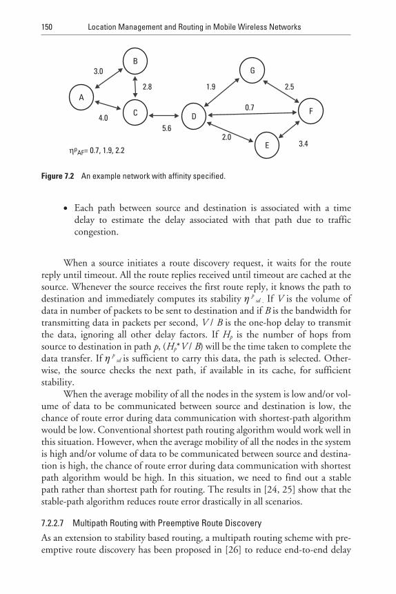
• Each path between source and destination is associated with a timedelay to estimate the delay associated with that path due to trafficcongestion.

When a source initiates a route discovery request, it waits for the routereply until timeout. All the route replies received until timeout are cached at thesource. Whenever the source receives the first route reply, it knows the path todestination and immediately computes its stability η p

sd . If V is the volume ofdata in number of packets to be sent to destination and if B is the bandwidth fortransmitting data in packets per second, V / B is the one-hop delay to transmitthe data, ignoring all other delay factors. If Hp is the number of hops fromsource to destination in path p, (Hp*V / B) will be the time taken to complete thedata transfer. If η p

sd is sufficient to carry this data, the path is selected. Other-wise, the source checks the next path, if available in its cache, for sufficientstability.

When the average mobility of all the nodes in the system is low and/or vol-ume of data to be communicated between source and destination is low, thechance of route error during data communication with shortest-path algorithmwould be low. Conventional shortest path routing algorithm would work well inthis situation. However, when the average mobility of all the nodes in the systemis high and/or volume of data to be communicated between source and destina-tion is high, the chance of route error during data communication with shortestpath algorithm would be high. In this situation, we need to find out a stablepath rather than shortest path for routing. The results in [24, 25] show that thestable-path algorithm reduces route error drastically in all scenarios.

7.2.2.7 Multipath Routing with Preemptive Route Discovery

As an extension to stability based routing, a multipath routing scheme with pre-emptive route discovery has been proposed in [26] to reduce end-to-end delay


A

C

G

F

E

D

B

2.5

0.7

3.42.0

5.6

2.8

4.0

3.0

1.9

ηpAF= 0.7, 1.9, 2.2

Figure 7.2 An example network with affinity specified.

and to ensure better quality of service. The successful operation of an ad hocnetwork will be disturbed, if an intermediate node, supporting a communica-tion between a source-destination pair, moves out of range during data transfer.This interruption in communication results in subsequent route rediscoverybetween that source-destination pair or invoking some path-maintenance algo-rithm that eventually increases the end-to-end delay.

Moreover, the routing schemes proposed so far in the context of ad hocnetworks employ single-path routing that might not ensure optimal end-to-enddelay. However, once a set of paths between s to d is discovered, in some cases, itis possible to improve end-to-end delay by splitting the volume of data into dif-ferent blocks and sending it via selected multiple paths from s to d which wouldeventually reduce congestion and end-to-end delay.

In [26], a mechanism is proposed for adaptive computation of multiplepaths in temporal and spatial domain to transmit large volume of data from s tod in ad hoc wireless networks. Two aspects are considered in this framework.The first aspect is to perform preemptive route rediscoveries before the occur-rence of route errors while transmitting large volume of data from s to d. Conse-quently, this helps to find out dynamically a series of multiple paths in thetemporal domain to complete the data transfer. The second aspect is to selectmultiple paths in the spatial domain for data transfer at any instant of time andto distribute the data packets in sequential blocks over those paths in order toreduce congestion and end-to-end delay. A notion of link stability and path sta-bility has been used [24] and a unified mechanism is proposed to address thesetwo aspects that relies on evaluating a path based on link stability and path sta-bility. The solution method uses Lagrangean relaxation and subgradient heuris-tics [27] to find out the paths and data distribution into those paths both intemporal and spatial domains. The performance of this approach has beenevaluated on a simulation environment. It has been observed that the use oftemporal multipaths allows any source to transmit a large volume of data to adestination without degradation of performance due to route-errors. Addition-ally, the use of spatial multipaths would help to significantly reduce the end-to-end delay and the number of route-rediscovery needed in this process.

In Figure 7.3, we have shown the stability of most stable path between twoarbitrary nodes, 14 and 5, of an ad hoc network, sampled at 5-second intervalsof time. At each 5 seconds, a route discovery process is initiated from node 14and the paths obtained after route-request–timeout (300 msec) are evaluated tofind out the most stable path. As shown in the figure, it has been observed thatno single path is stable throughout the span of 30 seconds. However, we are get-ting a sustained stability between node 14 and 5 through different intermediatenodes. This establishes the viability of our scheme. In other words, if we can per-form preemptive route rediscoveries before the occurrence of route errors whiletransmitting large volume of data from s to d, it is possible to find out


dynamically a series of multiple paths in temporal domain to complete a largevolume of data transfer.

7.2.2.8 Location-Aided Routing (LAR) Protocols

Location-Aided Routing (LAR) Protocols [28] suggest an approach to decreaseoverhead of route discovery by utilizing location information for mobile hosts.Such location information may be obtained using the global positioning system(GPS) [29]. The LAR protocols use location information to reduce the searchspace for a desired route. Limiting the search space results in fewer route discov-ery messages.

These protocols limit the search for a route to the so-called request zone,determined based on the expected location of the destination node at the time ofroute discovery. The expected zone of node D, from the viewpoint of node S attime t1, is the region that node S expects to contain node D at time t1. Node Scan determine the expected zone based on the knowledge that node D was atlocation L at time t0. If node S does not know a previous location of node D,then node S cannot reasonably determine the expected zone—in this case, theentire region that may potentially be occupied by the ad hoc network is assumedto be the expected zone. In this case, this algorithm reduces to the basic floodingalgorithm. In general, having more information regarding mobility of a destina-tion node, can result in a smaller expected zone.

During route discovery, the source node S defines (implicitly or explicitly)a request zone for the route request. A node forwards a route request only if it


0

2

4

6

8

10

12

0 5 10 15 20 25 30

Time (sec.)

Stab

ility

(inse

c.) o

f pat

hsfro

mno

de14

tono

de5

atev

ery

5se

c.in

terv

al

14-20-5

14-23-5

14-17-11-5

14-23-17-11-514-28-5

14-28-9-5

14-9-5

Figure 7.3 Stability of maximum stable path between node 14 and 5, sampled at each5-second interval (the path is given in the boxes).

TEAMFLY

Team-Fly®

belongs to the request zone (unlike the flooding algorithm). To increase theprobability that the route request will reach node D, the request zone shouldinclude the expected zone (described above). Additionally, the request zone mayalso include other regions around the request zone. Note that the probability offinding a path (in the first attempt) can be increased by increasing the size of theinitial request zone. However, route discovery overhead also increases with thesize of the request zone. Thus, there exists a trade-off between latency of routedetermination and the message overhead.

In this protocol, any intermediate node I detecting routing failure (due toa broken link) informs the source node S by sending a route error packet. Then,S initiates a new route discovery (using a request zone) to find a path to the des-tination D. The latency of route redetermination for node D can be improvedby allowing any intermediate node I detecting route error to initiate a route dis-covery using a request zone based on its own location information for node D.Such a local search may result in a smaller request zone because node I may becloser to D than S. Smaller request zone could reduce routing overhead. Thetime to find the new path to D may also be reduced, as a smaller request zone issearched.

7.2.2.9 Query Localization Techniques for On-Demand Routing

The on-demand protocols discover routes via a flooding technique, where thesource (or any node seeking the route) floods the entire network with a querypacket in search of a route to the destination. Flooding is straightforward toimplement. However, as mentioned before, network-wide flooding incurs aconsiderable overhead and diminishes the performance advantage of on-demandprotocols. The primary goal of this technique [30] is to investigate newapproaches to reduce the routing overhead by localizing the query flood to alimited region in the network. Similar ideas were explored before. The mostprominent among them is the location-aided routing or LAR technique dis-cussed above, which uses the GPS to limit the query flood to a restricted region.However, the approach presented in [30] makes intelligent use of routing histo-ries and does not need location information. On the other hand, it delivers com-parable performance advantage.

The proposed query localization protocols are based on the notion of spa-tial locality: “A mobile node cannot move too far too soon.” Thus, prior routinghistories can be cached to estimate a small region in the network with high prob-ability of finding the destination node. Only this region needs to be flooded. Inthis approach, prior route histories are used to limit the query to a region in theneighborhood of the prior routes. Hopwise distance is used to define the neigh-borhood. The following two heuristics are used in this protocol:


• Exploiting path locality: This approach relies on the assumption thatafter a route to the destination node breaks, the new route cannot bevery different than the most recently used route.

• Exploiting node locality: The assumption here is that the destinationnode can be found within a small number of hops from some node onthe most recently used route.

It is also possible in rare occasions that the route discovered is not theshortest route. This is possible because there is no guarantee that the shortestroute will be contained entirely within the request zone. This will increase theend-to-end delay of the data packets, which will now go via a suboptimal route.However, the performance evaluation shows that the overall savings obtained bythe reduction in routing overheads are much more significant and can actuallycontribute to lower delays.

7.2.3 A Mobile Agent-Based Protocol for Topology Discovery and Routing

7.2.3.1 A Mobile Agent-Based Framework for Topology Discovery

Mobile agents are a novel effective paradigm for distributed applications, andare particularly attractive in a dynamic network environment involving partiallyconnected computing elements. The notion of computation mobility againstconventional data mobility governs the underlying philosophy of agencies [31].Most research examples of the mobile agent paradigm as reported in the currentliteratures have two general goals: reduction of network traffic and asynchro-nous interaction. Some authors have suggested that agents can be used to imple-ment network management and to deliver network services [32]. Intensiveresearch on the “Insect-like Systems” has been done over the last few years. Themobile agent systems have been popularly simulated in close resemblance to anant colony [33]. Of particular interest is a technique for indirect interagent com-munication, called stigmergy, in which agents populate information cache ofnodes, which other agents can use [34]. Stigmergy serves as a robust mechanismfor information sharing.

In [35], the issues of geographical-position discovery in ad hoc networksthrough the implementation of a mobile multiagent-based framework have beeninvestigated and a connection management protocol has been proposed. Theprimary objective of this mobile multiagent framework is to asynchronously col-lect network topology information (e.g., node velocity, node location) and dis-tribute them into the information cache of all other nodes. In other words, anagent based information exchange and navigation protocol (proactive in nature)has been developed in order to make each node in the network aware of thepositions of all other nodes in the network, without consuming large portion of


network capacity. GPS support has been used at each node for the extraction ofgeographical coordinates, velocity, and direction of movement of each node.This location-awareness gives each node an approximate perception of the net-work topology. Based on this perception, an adaptive routing protocol has beendesigned ensuring the system to manage an uninterrupted connection in a dis-tributed fashion between any source and destination.

7.2.3.2 Basic Mechanism

Mobile agents or messengers that hop around in the network are a novel solu-tion to the problem of topology discovery. The agents hop from node to node,collect information from these nodes, meet other agents in their journey, inter-act with both to collect updates of parts of the network that they have not visitedor have visited a long time back, and gift these collected data sets to newly vis-ited nodes and agents. A node therefore receives updated information about thenetwork, from the agents visiting them at short regular intervals. Initially whenthe network commences, all the nodes are just aware of their own neighbors andare in a don’t-know state regarding the other nods in the system. However withagent navigation beginning, the nodes slowly get information about the othernodes and their neighbors.

For example, let us assume that an agent migrates at every K time tickbetween nodes. At time t0, each of the nodes has only information about theirimmediate neighbors. At time = t0 + T, an agent jumps to a node with the infor-mation that it has about its previous host node. Thus this node now has dataabout a new neighboring node and its neighbors (since the agent has carried thisinformation to it). In the next T time tick, a node gets information regardingtwo more nodes from another agent. It is to be noted that by controlling T (alsoknown as time to migrate, or TTM), it is possible to control the agent traffic inthe network. Moreover, the agent would always migrate from a node to only oneof its neighbor after T time-tick. So, the network would never get flooded withpropagation of agents [34].

A major aspect underlying the infiltration of topology information intomobile nodes is that the information carried must be recognized with a degree ofcorrectness. Since the agent navigation is asynchronous and there is an obvioustime gap between the procurement of information by an agent from one nodeand its delivery by the same agent to another node, it becomes imperative tointroduce a concept of recency of information. For example, let us assume twoagents A1 and A2 arrive at node n, both of them carrying information about nodem which is multihop away from node n. In order to update the topology infor-mation at node n about node m, there has to be a mechanism to find out whocarries the most recent information about node m: agent A1 or A2? To imple-ment that, every node in the network has a counter that is initialized to 0. Whenan agent leaves a node after completing all its tasks at the node, it increments the


counter by one. This counter gives the value of recency. At any point of time,the magnitude of the recency of any node represents the number of times thatnode was visited by agents since the commencement of the network. This alsoimplies that if two agents have a set of data concerning the same node, say nodem, then the agent carrying the higher recency value of node m has more currentinformation about it.

The primary aim of an agent is to collect all topology-related informationfrom its host node in the network and carry them periodically (as updates) toother nodes without flooding the network with topology-update packets. At aperiodic interval, an agent propagates its perception of the topology-information to only one of its neighbors, based on a least-visited neighbor-firstcriterion [34]. At each node, an agent monitors recency of its neighbors todecide which of them has received the least number of agent visits. The neigh-boring node that has received least number of agent visits so far will be the targetnode for the agent. Thus, an agent always migrates to a node, which has had theleast number of agent visits among the members of the network. Since the agentnavigation is a distributed protocol, it attempts to visit all nodes in the networkwith equal frequency. This in turn facilitates homogeneous topology-awareness.

In Figure 7.4, the text boxes at the bottom displays the time tick, the aver-age topology deviation, the number of agents in the system, the number ofnodes, the transmission range and the mobility of the system. In the inset, thelocal topology perception of the node 9 is shown. This window has beeninvoked by clicking on node 9 during the execution of the simulator. The nodesshown in black in the inset represents the positions of the nodes as perceived bynode 9 and the nodes in white depict the actual position of the nodes in the net-work topology.

7.2.3.3 Uninterrupted Connection Management

This topology-awareness discussed above leads to a scenario where conventionalroute discovery is no longer necessary. More explicitly, the nodes can now deter-mine the most stable route locally and initiate the sending of data packetsthrough it. The way to calculate the stability of a path is indicated [24]. After apoint of time, if the source node finds that the chosen route has attained a lowstability (indicating that it would soon cease to exist), the node computes a new,more stable route from the local information cache and redirects data packetsthrough the later. This adaptive route selection facilitates continuous communi-cation through multiple paths in the temporal domain. Thus, as long as twonodes remain connected, they will always be able to get at least one routethrough which communication can continue. In the case of multiroute avail-ability, the best route can always be selected. Quite perceivably, the adaptiveselection of best routes guarantees an uninterrupted communication sessionbetween two nodes thus ensuring multimedia data transfer to occur.


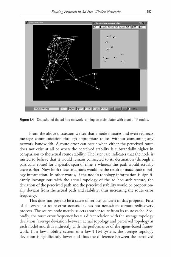
From the above discussion we see that a node initiates and even redirectsmessage communication through appropriate routes without consuming anynetwork bandwidth. A route error can occur when either the perceived routedoes not exist at all or when the perceived stability is substantially higher incomparison to the actual route stability. The later case indicates that the node ismisled to believe that it would remain connected to its destination (through aparticular route) for a specific span of time T whereas this path would actuallycease earlier. Now both these situations would be the result of inaccurate topol-ogy information. In other words, if the node’s topology information is signifi-cantly incongruous with the actual topology of the ad hoc architecture, thedeviation of the perceived path and the perceived stability would be proportion-ally deviant from the actual path and stability, thus increasing the route errorfrequency.

This does not pose to be a cause of serious concern in this proposal. Firstof all, even if a route error occurs, it does not necessitate a route-rediscoveryprocess. The source node merely selects another route from its route cache. Sec-ondly, the route error frequency bears a direct relation with the average topologydeviation (average deviation between actual topology and perceived topology ateach node) and thus indirectly with the performance of the agent-based frame-work. In a low-mobility system or a low-TTM system, the average topologydeviation is significantly lower and thus the difference between the perceived


Figure 7.4 Snapshot of the ad hoc network running on a simulator with a set of 14 nodes.

topology and the actual is less. If the source node takes care of this fact duringadaptive route selection, the chance of route errors would be reduced.

7.2.4 Power-Aware Routing Protocols in Ad Hoc Networks

7.2.4.1 Transmission Power Control in Ad Hoc Networks

Past work on power control has primarily dealt with cellular networks for man-aging cochannel interference at receivers and increasing network capacitythrough frequency reuse [36]. Essential to power control in this context is onlinelink quality monitoring for adaptation to changes induced by mobility andchannel impairments. Several power control algorithms have been presentedwith the following objectives:

• Increased power savings at mobile nodes;

• Better maintenance of stable QoS on wireless links;

• More efficient handling of mobility (structural stretching and hand-offs);

• Reduced interference on other links sharing the channel to enhancenetwork capacity.

The use of a power-control paradigm in ad hoc networks is relatively new.The problem of minimum energy routing or power-aware routing in ad hocnetworks has been addressed in [37, 38]. One of the approaches has been tominimize the total consumed energy in reaching the destination, which mini-mizes the energy consumed per unit flow or packet [37]. This approach maydrain out the batteries of certain paths, which may disable further informationdelivery even though there are many nodes with plenty of energy. Anotherapproach is to maximize the system lifetime given the sets of origin and destina-tion nodes and the information generation rate at the origin nodes. In yetanother approach [39], a new multiaccess protocol has been proposed. Radiosthat are not actively transmitting or receiving a packet switch themselves offwithout affecting the throughput. All these approaches have been shown toachieve their objective of energy conservation; however, they do not concernthemselves with the mechanism of transmit power control to optimize networkperformance.

Recently, two power-controlled MAC protocols (PCMAs) have been pro-posed [40, 41] in ad hoc networks. In [40], a PCMA is proposed where a senderwill use an appropriate power level to transmit its packets so as to increases thechannel utilization and save battery power. They have shown that the channelutilization can be significantly increased because the severity of signal


overlapping is reduced. In [41], a PCMA within the collision avoidance frame-work has been proposed. They have demonstrated that PCMA can allow morenumber of simultaneous communication than 802.11 by adapting the transmis-sion ranges to the minimum value required to satisfy successful reception at theintended destination. However, the main focus of both the works is to demon-strate the channel utilization using transmit power control. How to maintain atopology and how to incorporate a reactive routing scheme using power controlhas not been addressed. For example, connectivity in an ad hoc network needsto be maintained with suitable power control mechanism, even if there is nocommunication. And, a reactive routing protocol has to operate on that con-trolled topology. To address this problem, several researchers have investigatedthe issue of topology control in ad hoc networks, as discussed below.

7.2.4.2 Topology Control in Ad Hoc Networks by Adjusting Transmission Power

The topology of an ad hoc wireless network is the set of communication linksbetween node pairs and is primarily dependent on the transmission range ofindividual nodes. Normally, it is assumed that the transmission range is fixedand is a given parameter. However, it has been observed that a low transmissionrange will not guarantee proper connectivity among mobile hosts to ensureeffective communication. On the other hand, if the transmission range is high,it will ensure connectivity but will decrease channel utilization [40] and increasecollision and congestion of control packets [24], which will increase the end-to-end delay significantly. Hence, for a fixed transmission range, if the node den-sity is low, the network would be partitioned into disjoint components andproper network connectivity cannot be ensured. On the other hand, if the nodedensity is high, poor channel utilization and congestion and collision due tocontrol packets will degrade the network performance.

Adaptive adjustment of transmission power of each individual node cancontrol the topology of the network [42, 43]. Here, the objective of each nodein the network is to keep its number of neighbors bounded. Usually, duringroute-discovery phase, a source node broadcast a route-request packet thatpropagates from node to node and mainly responsible in generating the largenumber of control packets in the system. If Gavg is the average number of neigh-bors of a node and if the maximum number of hops is limited to 4, then theapproximate number of route-request control packets generated will be G 4

avg

communication event. Therefore, it is obvious that with increase in Gavg, thenumber of route-request control packets increases drastically. For a fixed trans-mission range, the number of control packets generated increases drasticallybeyond a certain node density, as it increases Gavg. However, if the transmissionrange is adjusted to keep the average number of neighbors bounded, the numberof route-request control packets generated would be uniform. Moreover, controlof transmission range will improve channel utilization by allowing more number


of simultaneous communications. At the same time, this strategy will also helpto increase the probability of a connected network to a large extent.

In a recent work on topology control, Ramanathan and Rosales-Hain [43]have addressed the issue of topology control in ad hoc wireless network usingtransmit power adjustment. For mobile ad hoc networks, they have presentedtwo distributed heuristics that adaptively adjust a node’s transmit powers inresponse to topological changes. Their results show that the performance ofmultihop wireless networks in practice can be substantially increased with topol-ogy control. In our paper, we will discuss only on the first heuristic, namely localinformation no topology (LINT). The second one, local information link-statetopology (LILT), depends on the global topology information that needs to beavailable with some proactive routing protocols such LSPs. However, manyresearchers feel that the proactive protocols, where each node tries to capture theglobal topology information, are not suitable in highly dynamic environment ofad hoc networks. Moreover, in LILT, an excessive number of topology control-induced updates will be generated that will propagate globally and decrease thethroughput of the network. Hence, we will not take into account LILT in ourpaper and discuss only LINT.

LINT attempts to keep the degree (number of neighbors) of each nodebounded. If the node degree is less than certain threshold, the node will increaseits transmission range. If the node degree is more than certain threshold, it willdecrease its transmission range. Thus, the basic mechanism of LINT depends onthe calculation of a node degree. It is assumed that the number of neighbors(degree) of any node will be known from its neighborhood table (built by somerouting mechanism). It has also been assumed that some neighborhood discov-ery protocol will return only bidirectional links. However, there is a significantshortcoming in these assumptions. In all reactive routing in ad hoc network, anode n will be aware of its neighbor only through a link-level beacon exchangefrom its neighbors. In other words, each node periodically broadcast a beacon tonotify its existence. Thus, the number of beacon a node n will receive will deter-mine the neighborhood counts of n, provided those nodes are also reachablefrom n (to ensure bidirectionality). At the same time, the number of beacons anode n will receive does not depend on the transmission range of n but on thetransmission range of other nodes. So, even if we increase the transmission rangeof n, it does not imply that it would increase the number of neighbors of n. As aconsequence, a node in the system may increase its transmission range indefi-nitely without increasing its number of bidirectional neighbors, simply becauseother nodes may not have any incentive to increase their transmission range. So,degree of a node n can only be calculated and manipulated, if there is a kind ofhandshaking between a node n and its intended neighbors to establish a neigh-borhood agreement. As a result, both n and its prospective neighbors have to


manipulate their transmission ranges in order to maintain a desirednumber of neighborhood relationships [42].

Another limitation of LINT is in its assumption of uniform node distribu-tion. Based on this assumption, the targeted value of transmit power for eachnode to attain a desired degree is calculated. However, uniform distribution isnot a realistic assumption. Moreover, no adaptive mechanism has been incorpo-rated to correct or rectify this assumption. We have incorporated an adaptivemechanism to adjust transmission range until the desired degree (in bidirec-tional sense) is actually achieved.

7.2.4.3 Selecting Optimal Transmission Range

The selection of optimal transmission range to maximize throughput and ensureconnectivity is studied in [44, 45]. Under certain assumptions, they havederived an optimal node-degree, called magic number. Assuming uniform dis-tribution, if the average node density is λ and AR is the area of coverage of node ifor transmission range R ( = ΠR 2 ), then the optimal value of λ. AR which maxi-mizes throughput has been referred to as magic number. It has been shown thatthe value of λ. AR from six to eight will have a high probability of leading to aconnected network as well as reducing congestion and collision in the network.Philips et al. [46] further conjectured that given a very large area, no fixed opti-mal number as magic number can exists. To ensure network connectivity, it hasbeen shown that the expected number of nearest neighbor (node degree) mustgrow logarithmically with the area of the network. They have shown that nodedegree should be between 2.195 and 10.526 to have a connected network withnonzero probability. Gupta et al. [47] addressed asymptotic connectivity of adhoc network under infinite node environment. Kirousis et al. [48] studied theproblem of assigning transmission ranges to the nodes of a multi hop network soas to minimize the total power consumption under the constraint of ensuring aconnected network. Sanchez et al. [49] and Elizabeth et al. [50] reported simula-tion results on critical range and impact of transmission range on throughput.All the analytical studies on connectivity assume uniform distribution. Theproblem becomes analytically intractable in case of nonhomogeneous distribu-tion of nodes. Moreover, if there is a large number of nodes in a large area,maintaining connectivity with very high probability can lead to a large transmis-sion range [51].

For a fixed number of nodes uniformly distributed over an operating area,an optimal transmission range can be worked out. But this would give a theo-retical solution only. In practice, if we consider a dynamic ad hoc network envi-ronment, the number of nodes as well as the concentration of node in differentarea of the operating zone varies. Therefore, a single, optimal transmissionrange, even if we find it, will not be a solution in this context. A protocol based


on variable transmission range would be highly effective in such a dynamic envi-ronment. It has been observed that [42] when nodes are randomly distributed ina finite plane with nonhomogeneous node distribution and the node degree ismaintained between 4 and 8 (with an average value of 6, the magic number) byadjusting the transmission range of individual node, it can ensure a connectednetwork with a probability of 96%.

7.2.4.4 A Routing Protocol with Adaptive Transmission Range Control

A routing protocol proposed with adaptive transmission range control [42] is anon-demand reactive protocol. The protocol has four components:

1. Transmission Range Control Protocol (TRCP), which will help eachnode to adjust periodically its transmission range in order to maintainthe number of its registered neighbors within four to eight;

2. Power-Sensitive MAC Protocol (PMAC), which controls medium accessin an environment where transmission range of each user terminal isvariable;

3. Path Finding Protocol (PFP), which is a demand-driven, source-initiated routing protocol to find a set of paths between any source-destination pair;

4. Path Evaluation and Data Communication Protocol (PEDCP), whichhelps the source to evaluate the best path among the set of paths andto start the data communication along that path. Additionally, ithelps TRCP to protect the links in the path during datacommunication.

The proposed protocol is based on a neighborhood agreement and denialscheme through periodic beacon exchange among the neighboring nodes only.The basic assumption is that, even if a node is within the transmission range ofanother node, it will not be considered as its neighbor unless both of them agreeto be the neighbor of each other. This ensures bidirectionality of neighborhoodrelationship. On the other hand, a node can increase its transmission range toinclude someone as its neighbor. A node will vary its transmission range so thatthe average number of its registered neighbor is around six. It has been pointedout earlier [44, 45] that if the average number of neighbors were six (the magicnumber), it would optimize the throughput by reducing congestion and colli-sion as well as ensuring connectivity of the network.

During routing of data packets, a node-pair will try to maintain theirneighborhood relationship by adjusting the transmission range, that is, protectthe link between them, if that link is involved in a communication process atthat instant of time. A source would evaluate a set of paths after route discoveryand find out the best path for data communication. The best path is a path


TEAMFLY

Team-Fly®

where the path protection mechanism during data communication will con-sume the least battery power during the adjustments of their transmission range.This is in tune with the concept of active link protection with power control incellular network [52]. In those schemes, the transmitter power is adjusted inorder to maintain the link quality and preserve the network topology understructural stretching (elastic network). One of the problem is that, some powersmay increase excessively and links become too expensive to maintain. That iswhy a path evaluation mechanism is used to find out the best path in thiscontext.

7.2.5 Other Routing Protocols

Zone Routing Protocol (ZRP) [53] is a zone- or cluster-based hybrid routingprotocol suitable for a wide variety of mobile ad hoc networks, especially thosewith large network spans and diverse mobility patterns. Each node proactivelymaintains routes within a local region (referred to as the routing zone). Knowl-edge of the routing zone topology is leveraged by the ZRP to improve the effi-ciency of a reactive route query and reply mechanism. The proactivemaintenance of routing zones also helps improve the quality of discoveredroutes, by making them more robust to changes in network topology. The ZRPcan be configured for a particular network by proper selection of a singleparameter, the routing zone radius. However, ZRP should be viewed more as arouting framework rather than an independent protocol, as potentially any pro-active protocol can be employed for intrazone (or, intracluster) routing and anyreactive protocol can be employed for interzone (or, intercluster) routing.

In ZRP, each node has its own routing zone, which includes the nodeswhose distance (hops) is at most some predefined number. Each node isrequired to know the topology of the network within its routing zone only, androute updates are propagated only within the routing zone. A proactive protocolsuch as DSDV is used within the routing zone to learn about its topology. Todiscover a route to an out-of-zone nodes, a reactive protocol such as DSR isused. Note that ZRP exhibits hybrid behavior of proactive and reactive throughthe use of the zone radius. For large zone radius, ZRP is more proactive, and forsmall zone radius, ZRP is more reactive. The route discovery requires a relativelysmall number of query messages as these messages are routed only to peripheralnodes, omitting all the nodes within the routing zones. This method is calledbordercasting.

The advantage of ZRP is that it significantly reduces the communicationoverhead as compared to the pure proactive protocols since in ZRP each nodeneeds to know the topology of its zone only. In addition, ZRP discovers routesfaster than the pure reactive protocols since in ZRP only the peripheral nodesare queried in the route discovery process.


Basic and Hierarchical Spine Routing is a distributed algorithm used to find anapproximation to the minimum connected dominating set (MCDS) of an adhoc network [54]. Topological information is then gathered from non-MCDS nodes and propagated to all MCDS nodes. Each MCDS node runs anall-pair shortest path algorithm. A non-MCDS node can then request the routeinformation to a destination from an adjacent MCDS node. Since MCDSnodes propagate, store and run shortest path algorithm on the topological infor-mation, their communication, storage and computation burdens are heavy.Moreover, mobility management is complicated by the existence of MCDSnodes.

Hierarchical spine routing (HSR) is a two-level routing architecture used to solvethe scalability problem in basic spine routing (BSR). The network is dividedinto clusters. Each cluster head stores the topology of a cluster graph, the clustermembership table (it consists of cluster ID for each node) and the list of localboundary nodes (it shows clusters reachable for each boundary node). Withineach cluster, BSR is used. Between clusters, link-state routing is run on the clus-ter graph topology. Using distinct clustering, the impact on topological changeis localized. Moreover, the amount of time for spine construction and mainte-nance is reduced since clusters essentially run in parallel. The communicationand the storage overhead in some nodes can be greatly reduced. However, clus-ter heads, boundary nodes, and spine nodes take on heavy responsibilities.Therefore, the communication, storage and computation burdens are heavy inthose nodes. Mobility management becomes complicated and the reliability ofthe network decreases due to single point of failure.

Optimized Link-State Routing (OLSR) Protocol [55] is an optimization of the purelink-state algorithm tailored to the requirements of a mobile WLAN. The keyconcept used in the protocol is that of multipoint relays (MPRs). MPRs are theselected nodes, which forward the broadcast packets during the flooding pro-cess. This technique substantially reduces the packet overhead as compared topure flooding mechanism where every node retransmits the packet when it re-ceives the first copy of the packet. The protocol is particularly suitable for thelarge dense networks as the technique of multipoint relays works well in thiscontext.

Relative Distance Microdiscovery Ad Hoc Routing (RDMAR) Protocol [56] is highlyadaptive, bandwidth-efficient and scaleable. A key concept in its design is that protocolreaction to link failures is typically localized to a very small region of the network nearthe change. This desirable behavior is achieved through the use of a novel mechanismfor route discovery, called relative distance microdiscovery (RDM). The concept behindRDM is that a query flood can be localized by knowing the relative distance (RD)


between two terminals. Based on the RD, the query flood is then localized to a limitedregion of the network centered at the source node of the route discovery and withmaximum propagation radius that equals to the estimated relative distance. This abilityto localize query flooding into a limited area of the network serves to increase scalabilityand minimize routing overhead and overall network congestion.

7.3 Multicast Routing Protocols in Ad Hoc Networks

Multicast communication in the context of ad hoc networks is a very useful andefficient means of supporting group-oriented applications, where the need forone-to-many data dissemination is quite frequent in critical situations such asdisaster recovery or battlefield scenarios. Instead of sending data via multipleunicasts, multicasting reduces the communication costs by minimizing the linkbandwidth consumption and delivery delay [57].

Research in the area of routing in ad hoc wireless network has mostly con-centrated on designing effective routing schemes for unicast communication.Those routing algorithms were not designed with multicast extensions in mind.Therefore, they do not naturally support multicast routing solutions. Since fixednetwork multicasting is based on state in routers (either hard or soft), it is funda-mentally unsuitable for ad hoc network where topology is changing frequentlydue to unconstrained mobility. It has been shown that the performance of bothhard- and soft-state multicast tree maintenance mechanisms degrade rapidlywith increased mobility. Multicast protocols used in static networks, such asDistance Vector Multicast Routing Protocol (DVMRP) [58, 59], multicast openshorted path first (MOSPF) [60], core-based trees (CBT) [61], and protocol inde-pendent multicast (PIM) [62], do not perform well in ad hoc networks becausemulticast tree structures are fragile and must be readjusted as connectivitychanges. Furthermore, multicast trees usually require a global routing substruc-ture such as link-state or distance vector. The frequent exchange of routing vec-tors or link-state tables, triggered by continuous topology changes, yieldsexcessive channel and processing overhead. Thus, traditional multicastapproaches that rely on maintaining and exchanging multicast-related stateinformation are not suitable in highly dynamic ad hoc network with frequentand unpredictable changing topology.

To construct a multicast delivery path, multicast routing schemes need toprovide a way for the delivery path to adapt to changes in network topology aswell as to changes in group membership. They need to do this in a timely fash-ion, not wasting bandwidth by sending unwanted data to resigned members orfailing to forward multicast traffic to new members. State retention overhead forrouting needs to be minimized at each host.


To do multicasting, some way is needed to define multicast groups. Inconventional multicasting algorithms, a multicast group is considered as a col-lection of hosts, which register to that group. It means that, if a host wants toreceive a multicast message, it has to join a particular group first. When hostswant to send a message to such a group, they simply multicast the message to theaddress of that group. All the group members then receive the message. An easilyreconfigurable multicast tree topology is required since it can be dynamicallychanged by movement of group members. However, unfortunately, channeloverhead caused by tree reconfiguration updates tends to increase very rapidlywith mobility [63]. Sometimes, multicast flooding may be a better solution inad hoc networks.

Currently proposed ad hoc multicast routing schemes lie on a spectrumthat spans from pure Internet multicast routing based schemes to a pure flood-ing scheme. Internet multicast routing schemes, as it is currently, generallyrequire the routing nodes to maintain fairly large amount of state informationfor routing and to use processing power of hosts rather liberally. Feasibility ofsupporting continuous unlimited mobility is also a question with Internet rout-ing schemes. Only flooding control packets may support unlimited continuousmobility. Flooding will also reduce the amount of state information kept atmobile hosts, and will provide reliable and timely delivery.

The Forwarding Group Multicast Protocol (FGMP) [64] proposes a schemethat is a hybrid between flooding and source based tree multicast. The proposedmulticast protocol scheme keeps track not of links but of groups of nodes, whichparticipate in multicast packets forwarding. To each multicast group G is associ-ated a forwarding group FG. Any node in FG is in charge of forwarding (broad-cast) multicast packets of G. The nodes to be included in FG are electedaccording to members’ requests. Instead of data packets, small membershipadvertisement packets are used to reduce overhead caused by broadcasting.However, in order to advertise the membership, each receiver periodically andglobally flood its member information.

The Ad Hoc Multicast Routing Protocol (AMRoute) [65] creates a per-groupmulticast distribution tree using unicast tunnels connecting group members.The protocol has two main components: mesh creation and tree creation. Cer-tain nodes are designated as logical core nodes that initiate mesh and tree crea-tion; however, the core can migrate dynamically according to groupmembership and network connectivity. Logical cores are responsible for initiat-ing and managing the signaling component of AMRoute, such as detection ofgroup members and tree set up. Bidirectional tunnels are created between pairsof group members that are close together, thus forming a mesh. Using a subsetof available mesh links, the protocol periodically creates a multicast distributiontree. AmRoute assumes the existence of an underlying unicast routing protocoland its performance is influenced by the characteristics of the unicast routing


protocol being used. The AMRoute simulation runs on top of TORA [21] asunderlying unicast protocol. The network dynamicity was emulated by keepingnode location fixed and breaking/connecting links between neighboring nodes.Thus, the effect of actual node mobility on the performance is difficult to inter-pret. Moreover, the signaling generated by underlying unicast protocol (TORAin this case) is not considered in the measurements.

The Core-Assisted Mesh Protocol (CAMP) [66] generalizes the notion ofCBTs introduced for Internet multicasting into multicast meshes that havemuch richer connectivity than trees. A shared multicast mesh is defined for eachmulticast group. The advantage of using such meshes is to maintain the con-nectivity even while the network routers move frequently. CAMP consists ofthe maintenance of multicast meshes and loop-free packet forwarding oversuch meshes. Multicast packets for a group are forwarded along the shortestpath from sources to receivers defined within the group’s mesh. CAMP rebuildsmeshes at least as fast as CBT and PIM can rebuild trees. However, the effectof mobility on the performance has not been clearly evaluated. The topologyunder experimentation has 30 routers with high connectivity (an average of6 neighbors each) and at the most 15 routers out of 30 are assumed to bemobile.

The ad hoc multicast routing protocol utilizing increasing ID numbers,(AMRIS) [67] assigns an identifier to each node in a multicast session. Apremulticast session delivery tree rooted at a special node (by necessity a sender)in the session joins all the group members. The tree structure is maintained byassigning identifiers in increasing order from the tree root outward to the othergroup members. All nodes are required to process the tree set up and mainte-nance messages that are transmitted by the root periodically. It has beenassumed that most multicast applications are long-lived; therefore rapid routereconstruction is of greater importance compared to rapid route discovery. Theperformance of the proposed scheme has yet to be evaluated.

The On-Demand Multicast Routing Protocol, (ODMRP) [68] also uses amesh-based approach for data delivery and uses a forwarding group concept. Itrequires sources rather than destinations to initiate the mesh building by peri-odic flooding of control packets. It applies on-demand procedures to dynami-cally build routes and maintain multicast group membership. A soft-stateapproach is taken to maintain multicast group member. In networks where GPSis available, ODMRP can be made adaptive to node movements by utilizingmobility prediction. By using location and mobility information supported byGPS, route expiration time can be estimated and receivers can select the paththat will remain valid for the longest time. With the mobility predictionmethod, sources can reconstruct routes in anticipation of route breaks. Thisway, the protocol becomes more resilient to mobility. The price is, of course, thecost and additional weight of GPS.


A location-based multicast scheme has been proposed in [69] to decreasedelivery overhead of multicast packets, as compared to multicast flooding. Alocation-based multicast group has been defined as the set of nodes residing in ageographical multicast region. Thus, if a host resides within a specific area at agiven time, it will be automatically a member of the corresponding multicastgroup at that time. All the hosts in the multicast region should receive the mul-ticast packet. Such a multicast group may be used for sending a message that islikely to be of interest to everyone at a given location (or in a specified area). Thescheme attempts to reduce the forwarding space for multicast packets. Limitingthe forwarding space results in fewer multicast messages, while maintaining theaccuracy of data delivery comparable with multicast flooding.

Stability-based multicast routing [24] is based on the stability-based unicastrouting scheme described above. The mechanism comprises four sequentialsteps. First, source initiates a route discovery to get all the paths to individualdestinations; next, it selects the stable routes from them and constructs a sub-graph connecting source and destinations; next, source extracts multicast tree(s)from this subgraph; finally, source communicates data to destinations using themulticast tree(s). The proposed multicast routing mechanism depends only onlocal state information at source for constructing a multicast tree dynamicallyand is demand-driven in the sense that whenever a source needs to communicatewith a set of destinations belonging to a multicast group, it discovers the routesto the individual destinations and creates a multicast tree dynamically at sourcefor that given group. Stability-based multicast routing scheme proposed herewill ensure that the lifespan of the multicast tree so formed will be sufficient tocomplete the required volume of data transfer at that instant of time.

7.4 Performance Comparisons of Unicast and Multicast RoutingProtocols

The comparative analysis of major unicast routing protocols has been studiedextensively through simulation and performance evaluation in [15, 705073].The performance comparison study of ad hoc wireless multicast protocols hasbeen presented in [63]. In this section, we will discuss the summary of theirfindings.

7.4.1 Performance Comparisons of Major Unicast Routing Protocols

The performance of DSR and AODV, two prominent on-demand routing pro-tocols for ad hoc networks has been evaluated in [15]. A detailed simulationmodel has been developed to demonstrate the performance characteristics of thetwo protocols. The general observation from the simulation is that forapplication-oriented metrics such as delay and throughput, DSR outperforms


AODV in less stressful situations (i.e., a smaller number of nodes and lower loador mobility or both). AODV, however, outperforms DSR in more stressfulsituations, with widening performance gaps with increasing stress (e.g., moreload, higher mobility). DSR, however, consistently generates less routing loadthan AODV. The poor delay and throughput performances of DSR are mainlyattributed to aggressive use of caching, and lack of any mechanism to expire staleroutes or to determine the freshness of routes when multiple choices are avail-able. The mechanisms to expire routes and/or determine freshness of routes, willbenefit DSR’s performance significantly. Since AODV keeps track of activelyused routes, multiple actively used destinations also can be searched using a sin-gle route discovery flood to control routing load. In general, it was observed thatboth protocols could benefit (1) from using congestion-related metrics (such asqueue lengths) to evaluate routes instead of emphasizing the hopwise shortestroutes, and (2) by removing “aged” packets from the network. The aged packetsare typically not important for the upper layer protocol, because they will proba-bly be retransmitted. These stale packets do contribute unnecessarily to the loadin the routing layer.

In [71], a comprehensive performance evaluation of major proactive andreactive routing protocols has been presented. Steady state performance in termsof fraction of packets delivered, delay and routing load have been considered asthe performance metrics. Even with a packet-level simulation model the essen-tial aspects of the routing protocols are exposed. The key observations are as fol-lows. The proactive, shortest path protocols provide excellent performance interms of end-to-end delays and packet delivery fraction at the cost of higherrouting load. The on-demand protocols suffer from suboptimal routes as well asworse packet delivery fraction because of more dropped packets. However, theyare significantly more efficient in terms of the routing load. The multipath pro-tocol, TORA, did not perform well in spite of maintaining multiple redundantpaths. The overhead of finding and maintaining multiple paths and the proto-col’s sensitivity to the loss of routing packets seem to outweigh the benefitsof multiple paths. Also, the end-to-end delay performance is poorbecause of the loss of distance information. The routing load differentialsbetween all routing protocols reduce with large number of peer-to-peer conver-sations in the network. However, the other performance differentials are notaffected conclusively.

In this work [70], the results of a detailed packet-level simulation compar-ing four recent multihop wireless ad hoc network routing protocols has beenpresented. These protocols, DSDV, TORA, DSR, and AODV, cover a range ofdesign choices, including periodic advertisements versus on-demand route dis-covery, use of feedback from the MAC layer to indicate a failure to forward apacket to the next hop, and hop-by-hop routing versus source routing. Theyhave simulated each protocol in ad hoc networks of 50 mobile nodes moving


about and communicating with each other, and presented the results for a rangeof node mobility rates and movement speeds.

Each of the protocols studied performs well in some cases yet has certaindrawbacks in others. DSDV performs quite predictably, delivering virtually alldata packets when node mobility rate and movement speed are low, and failingto converge as node mobility increases. TORA, although the worst performer inthe experiments conducted in terms of routing packet overhead, still deliveredover 90% of the packets in scenarios with 10 or 20 sources. At 30 sources, thenetwork was unable to handle all of the traffic generated by the routing protocoland a significant fraction of data packets were dropped. The performance ofDSR was very good at all mobility rates and movement speeds, although its useof source routing increases the number of routing overhead bytes required bythe protocol. Finally, AODV performs almost as well as DSR at all mobilityrates and movement speeds and accomplishes its goal of eliminating source rout-ing overhead, but it still requires the transmission of many routing overheadpackets and at high rates of node mobility is actually more expensive than DSR.

7.4.2 Performance Comparisons of Major Multicast Routing Protocols

A performance evaluation and comparative analysis of five multicast protocolsfor ad hoc networks has been presented in [63]. The channel, radio, IEEE802.11 MAC protocol, and multicast protocols (AMRoute, ODMRP, AMRIS,CAMP, and flooding) have been carefully implemented The simulator has mod-eled a realistic wireless environment and results have been obtained for a broadrange of parameters including mobility, number of senders, multicast groupsize, and traffic load. A general conclusion is that, in a mobile scenario, mesh-based protocols outperformed tree-based protocols. The availability of alternateroutes provided robustness to mobility. AMRoute performed well under nomobility, but it suffered from loops and inefficient trees even for low mobility.AMRIS was effective in a light traffic environment with no mobility, but its per-formance was susceptible to traffic load and mobility. CAMP showed better per-formance when compared to tree protocols, but with mobility, excessive controloverhead caused congestion and collisions that resulted in performance degrada-tion. ODMRP was very effective and efficient in most of the simulation scenar-ios. However, the protocol showed a trend of rapidly increasing overhead as thenumber of senders increased.

7.5 Discussion

Several researchers feel that on-demand reactive routing schemes that do not useperiodic message of any kind would be more suitable in the context of ad hoc


networks. However, it has been observed that these protocols perform wellunder light traffic and low mobility, but performance degrades significantlyunder high mobility and high traffic load. As mobility increases, the precom-puted route may break down, requiring multiple route discoveries on the way todestination. Route caching becomes ineffective in high mobility. Stability-basedrouting schemes that tend to evaluate the lifespan of a path reduce this problem,but cannot eliminate it. Moreover, since flooding is used for query dissemina-tion and route maintenance, on-demand routing tends to become inefficientwhen the frequency of communication requirement is high.

On the other hand, several researchers have proposed proactive routingschemes based on classical DVR or LSR. The DVR approach is simple and com-munication overhead is less than that of LSR, but it suffers from slow conver-gence and the tendency to create routing loops. In LSR, global networktopology information is maintained in all routers by the periodic flooding oflink-state updates by each node. Any link change triggers an immediate update.As a result, the time required for a router to converge to the new topology ismuch less than in the distance vector approach. Due to global topology knowl-edge, preventing routing loop is also easier. Moreover, the link-state informa-tion to evaluate the quality of the entire path (e.g., bandwidth, delay, lifespan,affinity) can be easily obtained from the global topology information main-tained at each node. Unfortunately, as these schemes rely on flooding of routingupdates, excessive control overhead may be generated, especially in a highlymobile environment. Thus, in the context of ad hoc networks, researchers havefocused on restricting the propagation of routing updates, thereby reducing thecontrol overheads. For example, OLSR protocol is an optimization of the purelink-state algorithm tailored to the requirements of a mobile WLAN. The keyconcept used in the protocol is that of MPRs. MPRs are the selected nodes,which forward the broadcast packets during the flooding process. This tech-nique substantially reduces the packet overhead as compared to pure floodingmechanism where every node retransmits the packet when itreceives the first copy of the packet. FSR introduces the notion of multilevelfisheye scope to reduce routing update overhead in large networks. Nodesexchange link-state entries with their neighbors with a frequency that dependson distance to destination. From link-state entries, nodes construct the topologymap of the entire network and compute optimal routes.

Designing a proper routing scheme to suit different application contexts ofad hoc networks for efficient message communication along with power conser-vation is still a challenging task. With the advent of radios with more sophisti-cated controls on transmission parameters, adaptive transmission range is goingto be a viable commercial solution in near future. An energy-conserving routingprotocol with adaptive transmission range control may be a good candidate forfuture ad hoc networks.


References

[1] Perlman R., Interconnections: Bridges and Routers, Addison-Wesley, 1992, pp. 149–152,205–233.

[2] Jubin, J., and J. Tornow, “The DARPA Packet Radio Network Protocols,” Proc. of theIEEE 75(1), Jan. 21–32, 1987.

[3] McQuillan, John M., Ira Richer, and Eric C. Rosen, “The New Routing Algorithm forthe ARPANET,” IEEE Transactions on Communications, Vol. 28, No. 5, May 1980,pp. 711–719.

[4] Moy, J., “Multicast Routing Extensions for OSPF,” Communications of the ACM, Vol. 37,No. 8, Aug. 1994, pp. 61–66, 114.



[7] Pei, Guangyu, Mario Gerla, and Tsu-Wei Chen, “Fisheye State Routing: A RoutingScheme for Ad Hoc Wireless Networks,” Proc. of the IEEE International Conference onCommunication, New Orleans, LA, June 2000.

[8] Royer, E. M., and C. K. Toh, “A Review of Current Routing Protocols for Ad HocMobile Wireless Networks,” IEEE Personal Communications, Apr. 1999.

[9] Perkins, E., and P. Bhagwat, “Highly Dynamic Destination-Sequenced Distance-VectorRouting (DSDV) for Mobile Computers,” ACM Comput. Commun. Rev., Vol. 24, No. 4,(ACM SIGCOMM’94) Oct. 1994, pp. 234–244.

[10] Murthy, S., and J. J. Garcia-Luna-Aceves, “An Efficient Routing Protocol for WirelessNetworks,” ACM Mobile Networks and Applications J., Vol. 1, No. 2, 1996, pp. 183–197.

[11] Krishna, P., et al., “A Cluster-Based Approach for Routing in Ad Hoc Networks,” Proc. ofthe 2nd USENIX Symp. on Mobile & Location-Independent Computing, Apr. 1995.

[12] Chiang, C. C., and M. Gerla, “Routing in Clustered Multihop Mobile Wireless Net-works,” Proc. of 11th International Conference on Information Networking, Taiwan 1997.

[13] Kleinrock, L., and K. Stevens, “Fisheye: A Lenslike Computer Display Transformation,”technical report, UCLA, Computer Science Department, 1971.

[14] Johnson, B., and D. A. Maltz, “Dynamic Source Routing in Ad Hoc Wireless Networks,”T. Imielinski and H. Korth, (eds.) in Mobile Computing, Boston: Kluwer, 1996.

[15] Das, S R, Charles Perkins and Elizabeth Royer, “Performance Comparison of Two On-Demand Routing Protocols for Ad Hoc Networks,” Proc. of the IEEE INFOCOM 2000,Tel Aviv, Israel, March 26–30, 2000.

[16] Park, V. D., and M. S. Corson, “A Highly Adaptive Distributed Routing Algorithm forMobile Wireless Networks,” IEEE INFOCOM’97, Kobe, Japan, Apr. 1997.

[17] Perkins, E., “Ad Hoc On-Demand Distance Vector (AODV) Routing,” Internet Draft,Nov. 1997.


TEAMFLY

Team-Fly®

[18] Perkins, C. E., and E. M. Royer, “Ad Hoc On-Demand Distance Vector Routing”, Proc.of the 2nd IEEE Workshop on Mobile Comp. Sys. And Apps., Feb. 1999, pp. 90–100.

[19] Perkins, Charles, Elizabeth Royer, and Samir Das. “Ad Hoc On-Demand Distance Vector(AODV) Routing,” http:// www.ietf.org/ internet-drafts/ draft-ietf-manet-aodv-03.txt,June 1999, IETF Internet Draft (work in progress).

[20] Gafni, E., and D. Bertsekas, “Distributed Algorithms for Generating Loop-Free Routes inNetworks with Frequently Changing Topology,” IEEE Trans. Commun., Jan. 1981.

[21] Corson, M. S., and A. Ephremides, “A Distributed Routing Algorithm for Mobile Wire-less Networks,” ACM/Baltzer Journal on Wireless Networks, Vol. 1, No. 1, Feb. 1995,pp. 61–82.

[22] Toh, C. K., “A Novel Distributed Routing Protocol to Support Ad Hoc Mobile Comput-ing,” IEEE International Phoenix Conf. on Computer & Communications (IPCCC’96),1996.

[23] Dube, R., et al., “Signal Stability Based Adaptive Routing for Ad Hoc Mobile Networks,”Technical Report CS-TR-3646, UMIACS-TR-96-34, Institute for Advanced ComputerStudies, Department of Computer Science, University of Maryland, College Park,MD, Aug. 1996.

[24] Paul, Krishna, et al., “A Stability-Based Distributed Routing Mechanism to SupportUnicast and Multicast Routing in Ad Hoc Wireless Network,” Computer Communications(Elsevier Science), Vol. 24, Dec. 2001, pp. 1828–1845.

[25] Paul, Krishna, Romit Roychoudhuri, and S. Bandyopadhyay, “Survivability Analysis ofAd Hoc Wireless Network Architecture,” Proc. of the Second International Workshop onMobile and Wireless Communication Networks, Paris, France, May 2000. Published in Lec-ture Notes in Computer Science LNCS 1818, Springer Verlag.

[26] Das, Sajal K., et al., “Improving Quality-of-Service in Ad Hoc Wireless Networks withAdaptive Multipath Routing,” Accepted in GLOBECOM 2000, San Francisco, CA, Nov.27–Dec 1, 2000.

[27] Fisher, M. L., “An Applications Oriented Guide to Langrangean Relaxation,” Interfaces,Vol. 15, 1985, pp. 10–21.

[28] Ko, Y. B., and N. H. Vaidya, “Location-Aided Routing in Mobile Ad Hoc Networks,”Proc. of the ACM/IEEE MOBICOM 98, Oct. 1998.

[29] Imielinski, T., and J. C. Navas, “GPS-Based Addressing and Routing,” Tech. Rep.LCSR-TR-262, CS Dept., Rutgers University, March (updated Aug.) 1996.

[30] Castaneda, R., and S. R. Das, “Query Localization Techniques for On-Demand RoutingProtocols in Ad Hoc Networks,” Proc. of the 1999 ACM Mobicom Conference, Seattle,WA, Aug. 1999.

[31] Appeleby, Steve, and S. Steward, “Mobile Software Agents for Control in Telecommuni-cations Networks,” BT Technology Journal, Vol. 12, No. 2, Apr. 1994, pp. 104–113.

[32] Krause, S., and T. Magedanz, “Mobile Service Agents Enabling Intelligence on Demandin Telecommunications,” Proc. of the IEEE GLOBCOM ‘96, 1996.


[33] Schoonderwoerd, R., “Ant-Based Load Balancing in Telecommunications Networks,”Adaptive Behavior, Vol. 5, No. 2, 1997, pp. 169–207.

[34] Roy Choudhury, Romit, S. Bandyopadhyay, and K. Paul, “A Distributed Mechanism forTopology Discovery in Ad Hoc Wireless Networks Using Mobile Agents,” Proc. of theFirst International Workshop on Ad Hoc Networks, ACM/IEEE MobiHoc 2000, in conjunc-

tion with MobiCom 2000, Boston, MA 2000.

[35] Roy Choudhury, Romit, Krishna Paul, and S. Bandyopadhyay, “An Agent-Based Connec-tion Management Protocol for Ad Hoc Wireless Networks,” Journal of Network and Sys-tem Management, to appear.

[36] Bambos, Nicholas, “Towards Power-Sensitive Network Architecture in Wireless Commu-nications: Concepts, Issues and Design Aspects,” IEEE Personal Communications, June1998, pp. 50–59.

[37] Chang, Jae-Hwan, and L. Tassiulas, “Energy Conserving Routing in Wireless Ad HocNetworks,” in Proc. IEEE INFOCOM 2000, Vol. 1, 2000, pp. 22–31

[38] Singh, S., M. Woo, and C. S. Raghavendra, “Power-Aware Routing in Mobile Ad HocNetworks,” ACM MOBICOM, 1998, pp. 181–190

[39] Singh, S., and C. S. Raghavendra “Power Efficient MAC Protocol for Multihop RadioNetworks,” Proc. of IEEE PIRMC’98 Conf., Vol. 1, Sept. 1998, pp. 153–157.

[40] Wu, Shih-Lin, and Yu-Chee Tseng, “Intelligent Medium Access for Mobile Ad Hoc Net-works with Busy Tones and Power Control,” JSAC, Vol. 18, No. 9, Sept. 2000.

[41] Monks, Jeffrey P., Vaduvur Bharghavan, and Wen-Mei Hwu, “A Power Controlled Mul-tiple Access Protocol for Wireless Packet Networks,” IEEE INFOCOM 2001, Anchorage,AK, April 2001.

[42] Paul, Krishna, and S. Bandyopadhyay, “Self-Adjusting Transmission Range Control ofMobile Hosts in Ad Hoc Wireless Networks for Stable Communication,” Presented in theSixth International Conference on High Performance Computing HiPC99, Calcutta, India,Dec. 1999.

[43] Ramanathan, R., and R. Rosales-Hain, “Topology Control of Multihop Wireless Net-works Using Transmit Power Adjustment,” Proc. of the IEEE Conference on ComputerCommunications (INFOCOM), Tel Aviv, Israel, March 2000, pp. 404–413.

[44] Takagi, H., and L. Kleinrock, “Optimal Transmission Ranges for Randomly DistributedPacket Radio Terminals,” IEEE Trans. Commun., Vol. COM-32, pp. 246–257, March1984.

[45] Cheng, Y. C., and T. G. Robertazzi, “Critical Connectivity Phenomena in MultihopRadio Network,” IEEE Trans. Commun., 37, 1989, pp. 770–777.

[46] Philips, T., S. Panwar and A. Tantawi, “Connectivity Properties of a Packet Radio Net-work Model,” IEEE Transaction on Information Theory, Vol. 35, No. 5, Sept. 1989.

[47] Gupta, P., and P. R. Kumar, “Critical Power for Asymptotic Connectivity in WirelessNetworks,” Stochastic Analysis, Control, Optimization and Applications, W. M. McEneany,G. Yin, and Q. Zhang, (eds.), Boston, MA: Birkhauser, 1998, pp. 547–566.


[48] Kirousis, L. M., et al., “Power Consumption in Packet Radio Networks,” Theoretical Com-puter Science 243 (2000), pp. 289–305.

[49] Sanchez, M., P. Manzoni, and Z. Haas, “Determination of Critical Transmission Rangein Ad Hoc Networks,” IEEE Workshop on Multiaccess, Mobility and Teletraffic for WirelessCommunications, Oct. 1999.

[50] Royer, Elizabeth M., and Charles E. Perkins, “Transmission Range Effects on AODVMulticast Communication,” to appear in ACM Mobile Networks and Applications specialissue on Multipoint Communication in Wireless Mobile Networks.

[51] Lee, S., “Determining Transmission Range in Ad Hoc Networks”, Technical Report, Dept.of Computer Science, University of Maryland, College Park, MD, May 2001.

[52] Chen, S., N. Bambos, and G. Pottie, “On Power Control with Active Link Quality Pro-tection in Wireless Communications Networks,” IEEE Proc. 28th Annual Conf. on Infor-mation Sciences and Systems, 1994.

[53] Haas, Z. J., “The Zone Routing Protocol (ZRP) for Ad Hoc Networks,” Internet Draft,Nov. 1997.

[54] Das, B., R. Sivakumar, and V. Bharghavan, “Routing in Ad Hoc Networks Using a Vir-tual Backbone,” IEEE IC3N’97, Sept. 1997, pp. 1–20.

[55] Qayyum, Amir, Philippe Jacquet, and Paul Muhlethaler, “Optimized Link-State RoutingProtocol,” http://www.ietf.org/ internet-drafts/ draft-ietf-manet-olsr-01.txt, Feb. 2000.IETF Internet Draft (work in progress).

[56] Aggelou, G, and Rahim Tafazolli. “Relative Distance Micro-Discovery Ad Hoc Routing(RDMAR) Protocol,” http://www.ietf.org/ internet-drafts/ draft-ietf-manet-rdmar-01.txt,Sept. 1999, IETF Internet Draft (work in progress).

[57] Obraczka, K., and G. Tsudik, “Multicast Routing Issues in Ad Hoc Networks,” Proc. ofthe IEEE ICUPC ’98, Oct. 1998.

[58] Deering, S.E., and D. R. Cheriton, “Multicast Routing in Datagram Internetworks andExtended LANs,” ACM Transactions on Computer Systems, Vol. 8, No. 2, May 1990,pp. 85–110.

[59] Waitzman, D., S. Deering, and C. Partridge, “Distance Vector Multicast Routing Proto-col,” RFC 1075, Nov. 1988.

[60] Moy, J., “Multicast Routing Extensions for OSPF,” Communications of the ACM, Vol. 37,No. 8, Aug. 1994, pp. 61–66, 114.

[61] Ballardie, T., P. Francis, and J. Crowcroft, “Core Based Trees (CBT)—An Architecturefor Scalable InterDomain Multicast Routing,” Proc. of ACM SIGCOMM’93, San Fran-cisco, CA, Oct. 1993, pp. 85–95.

[62] Deering, S., et al., “The PIM Architecture for Wide-Area Multicast Routing,” IEEE/ACMTransactions on Networking, Vol. 4, No. 2, Apr. 1996, pp. 153–162.

[63] Lee, Sung-Ju, et al., “A Performance Comparison Study of Ad Hoc Wireless MulticastProtocols,” Proc. of the IEEE INFOCOM 2000, Tel Aviv, March 26–30, 2000.


[64] Chiang, Ching-Chuan, Mario Gerla, and Lixia Zhang, “Forwarding Group Multicast Pro-tocol (FGMP) for Multihop, Mobile Wireless Networks,” ACM-Baltzer Journal of ClusterComputing: Special Issue on Mobile Computing, Vol. 1, No. 2, 1998

[65] Liu, M., et al., “AMRoute: Ad Hoc Multicast Routing Protocol,” CSHCN TR 99–1,University of Maryland, College Park, MD.

[66] Garcia-Luna-Aceves, J. J., and E. Lmadruga, “A Multicast Routing Protocol for Ad HocNetworks,” Proc. of the IEEE INFOCOM’99, New York, March 1999.

[67] Wu, C. W., Y. C. Tay, and C. K. Toh, “Ad Hoc Multicast Routing Protocol UtilizingIncreasing ID-Numbers,” Internet-draft, draft-ietf-manet-amris-spec-00.txt, Nov. 1998.

[68] Lee, Sung-Ju, W. Su, and M. Gerla, “On-Demand Multicast Routing Protocol(ODMRP) for Ad Hoc Networks,” Internet-draft, draft-ietf-manet-odmrp-01.txt, June1999.

[69] Ko, Y. B., and N. H. Vaidya, “Location-Based Multicast in Mobile Ad Hoc Networks,”TR98-018, Deptartment of Computer Science, Texas A&M University.

[70] Broch , J., et al., “A Performance Comparison of Multi-Hop Wireless Ad Hoc NetworkRouting Protocols,” Proc. ACM/IEEE Mobile Comput. and Network., Dallas, TX, Oct.1998.

[71] Das, S. R., et al., “Comparative Performance Evaluation of Routing Protocols for Mobile,Ad Hoc Networks,’’ Proc. of IEEE IC3N’98, Lafayette, LA, Oct. 1998, pp. 153–161.

[72] Johansson, P., et al., “Scenario-Based Performance Analysis of Routing Protocols forMobile Ad Hoc Networks,” Proc. of ACM/IEEE MOBICOM’99, Seattle, WA, Aug. 1999,pp. 195–206.

[73] Lee, S. J., M. Gerla, and C. K. Toh, “A Simulation Study of Table-Driven And On-Demand Routing Protocols for Mobile Ad Hoc Networks,” IEEE Network, Vol. 13,No. 4, July 1999, pp. 48–54.


Part IIIFuture Issues

.

8Routing in Next-Generation WirelessNetworks

8.1 UMTS All-IP Networks

At the end of 1999, work started in 3GPP toward an all-IP architecture. Thisevolution was driven by two objectives:

1. Independence of the transport and control layer to ease the implemen-tation of new applications up to the mobile terminal;

2. Operation and maintenance optimization for the access network.

This evolution has an impact on different parts of the network. Basically,three main (and independent) evolutions are part of this evolution toward anall-IP architecture [1]:

• Evolution moves toward a next-generation network (NGN) type ofarchitecture in the circuit switch domain, where the MSC function issplit into a control plane part (MSC server) and a user plane part(media gateway). The introduction of packet transport (IP or ATMsince the network architecture is independent of the underlying trans-port layer) on the network subsystem (NSS) backbone also allows mov-ing the transcoder toward the border of the public land mobile network(PLMN). As such transcoder-free operation (TrFO) is possible, whichresults in much better voice quality. This feature is part of release 4.

179

• Addition of an IP-based multimedia subsystem (IMS) that introducesthe capabilities to support IP-based multimedia services, such as voiceover IP (VoIP) and multimedia over IP (MMoIP), and makes use of thepacket-switched network for the transport of control and user planedata. The PS domain also deals with all the mobility (handover) aspects.This feature is part of release 5.

• Introduction of IP transport technology within the UTRAN is an alter-native to the ATM-based UTRAN. This feature is also part of release 5.It is important to stress that these evolutions are independent of eachother and can also be deployed in a fully independent way. This meansthat for each of these evolutions the operator can make an independentyes or no decision.

The introduction of the IMS is driven by the demand to offer more andenhanced services to end users. It is clear that IP plays a major role in the quickintroduction of new services. Operators are faced with the challenge of findingtheir role in these new business opportunities. Based on their specific strengthssuch as expertise in communication and powerful billing systems, networkoperators are now moving into communication-oriented services. To do this,network infrastructures must be transformed into secure, open, and flexibleplatforms on which third-party developers and service providers can add genericas well as customized applications rapidly and cost effectively.

The main drivers leading this transformation of the value model of thepublic telecom market can be analyzed along three directions:

1. Provision of user-centric solutions: Market demand for services are evolv-ing from a standardized one-size-fits-all service to a fully customizedservice that adapts to the user’s choice and preference, as well as termi-nal and location.

2. Usage of the new capabilities of networks and terminals: Available band-width is increasing, which enables the deployment of media-rich serv-ices making use of all capabilities for interactivity. Control capabilityfor network resources is enabling provision of the adapted media to theuser with the expected levels of QoS and security.

3. Evolution of marketplace and business: With the shift in value chain,new roles are defined and new stakeholders are taking their place in themarket (service providers, service retailers). In parallel, deregulationand the need for timely coping with fierce competition fuel opennesstoward third parties and support for open service creation andprovision.


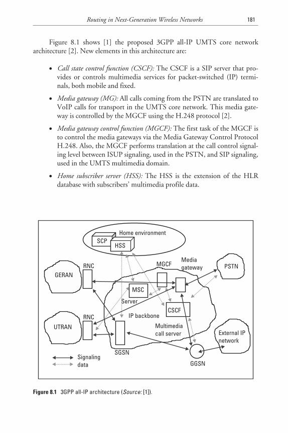
Figure 8.1 shows [1] the proposed 3GPP all-IP UMTS core networkarchitecture [2]. New elements in this architecture are:

• Call state control function (CSCF): The CSCF is a SIP server that pro-vides or controls multimedia services for packet-switched (IP) termi-nals, both mobile and fixed.

• Media gateway (MG): All calls coming from the PSTN are translated toVoIP calls for transport in the UMTS core network. This media gate-way is controlled by the MGCF using the H.248 protocol [2].

• Media gateway control function (MGCF): The first task of the MGCF isto control the media gateways via the Media Gateway Control ProtocolH.248. Also, the MGCF performs translation at the call control signal-ing level between ISUP signaling, used in the PSTN, and SIP signaling,used in the UMTS multimedia domain.

• Home subscriber server (HSS): The HSS is the extension of the HLRdatabase with subscribers’ multimedia profile data.

Routing in Next-Generation Wireless Networks 181

MediagatewayMGCF

SGSN

Multimediacall server

Server

GGSN

SCPHSS

Home environment

RNC

RNC

GERAN

UTRAN

MSC

CSCF

PSTN

External IPnetwork

IP backbone

Signalingdata

Figure 8.1 3GPP all-IP architecture (Source: [1]).

8.2 Routing in Distributed Wireless Sensor Networks

8.2.1 Introduction

Over the last few years, the design of micropower wireless sensor systems hasgained increasing importance for a variety of applications. We have observedmajor advances in the design of ultra-low power sensor systems based on infra-red, vibration and acoustic sensors. They combine micropower sensor technol-ogy with a low power sensor interface, signal processing and weak-inversion RFcircuits to implement entire sensor systems with the capability of forming wire-less networks. Collaboration is essential between sensor nodes for the fusion ofdata, and the organization of the nodes can be ad hoc. While efficient protocolshave been proposed to deal with ad hoc networks, large-scale wireless networkswith thousands of nodes are not usually considered in that research. Moreover,energy has not been explicitly used as a metric. The availability of energy from abattery or a large power source is not always a good assumption. For example,the monitoring devices can be embedded into objects where replacing the bat-tery is very inconvenient or impossible. The short life span of sensors and theirredeployment make the topology of sensor networks quite dynamic, and theseissues determine the chassis of adaptive approaches towards the design of rout-ing protocols of such large-scale networks [3].

8.2.2 Sensor Networks

Integrated low-power sensing devices will permit remote object monitoring andtracking in many different contexts: in the field (vehicles, equipment, person-nel), the office building (projectors, furniture, books, people), the hospital ward(syringes, bandages) and the factory floor (motors, small robotic devices). Net-working these sensors using their wireless communication capabilities, empow-ering them with the ability to coordinate among themselves on a larger sensingtask will revolutionize information gathering and processing in many situations.Large-scale, dynamically changing, and robust sensor colonies can be deployedin inhospitable physical environments such as remote geographic regions ortoxic urban locations. They will also enable low maintenance sensing in morebenign, but less accessible, environments, such as large industrial plants, and air-craft interiors.

To motivate the challenges in designing these sensor networks, considerthe following scenario. Several thousand sensors are rapidly deployed (e.g.,thrown from an aircraft) in remote terrain. The sensors coordinate to establish acommunication network, divide the task of mapping and monitoring terrainamong themselves in an energy-efficient manner, adapt their overall sensingaccuracy to the remaining total resources, and reorganize upon sensor failure.When additional sensors are added or old sensors fail, the sensors reorganize


TEAMFLY

Team-Fly®

themselves to take advantage of the added system resources. Several aspects ofthis scenario present systems design challenges different from those posed byexisting computer networks. The sheer number of these devices, and their unat-tended deployment, will preclude reliance on broadcast communication or theconfiguration currently needed to deploy and operate networked devices.Devices may be battery constrained or subject to hostile environments, so indi-vidual device failure will be a common event. In addition, the configurationdevices will frequently change in terms of position, reachability, power availabil-ity, and even task details. Finally, because these devices interact with the physicalenvironment, they, and the network as a whole, will experience a significantrange of task dynamics [3].

In sensor networks, most traffic is in the form of many-to-one data flowsbetween all the networked sensors and the monitoring node. Flooding, which isnormally used for disseminating information, can also be used for the networkor topology discovery. The monitoring node(s) initiate flooding by passing amessage to all its neighbors, each successive node forwarding it once. As floodingproceeds, nodes keep track of whom they received messages from. In case a nodereceives several copies of the same message from its neighbors it employs a par-ent selection algorithm to choose one of these as its parent. It then sends backinformation to its parent along the reverse direction of the original floodingmessage, when it needs to forward data back to a monitoring node. The networktopology that is thus discovered is a spanning tree. It is of interest to knowwhether the discovered tree is bushy, with a few large clusters or sparse, withmany smaller clusters.

In a network of thousands of nodes, it is unlikely that the designer willdetermine the position of each node. In an extreme case, nodes may be droppedfrom the air and scatter about an unknown area. To process sensor data, how-ever, it is imperative to know where the data is coming from. Nodes could beequipped with a GPS to provide them with knowledge of their absolute posi-tion, but this is currently a costly (in volume, money, and power consumption)solution. Instead, positional information can be inferred from connection-imposed proximity constraints. In this model, only a few nodes have knownpositions (perhaps equipped with GPS or placed deliberately) and the remainderof the node positions are computed from knowledge about communicationlinks [4].

8.2.3 Topology Maintenance and Sensor Deployment

Sheer numbers of inaccessible and unattended sensor nodes, which are prone tofrequent failures, make topology maintenance challenging task. Hundreds toseveral thousands of nodes are deployed throughout the sensor field. They aredeployed within tens of feet of each. The node densities may be as high as 20


nodes/m3. Deploying high number of nodes densely requires careful handling oftopology maintenance. We examine issues related to topology maintenance andchange in three phases [3]:

1. Predeployment and deployment phase: Sensor nodes can be eitherthrown in mass or placed one by one in the sensor field. They can bedeployed by dropping from plane, delivering in an artillery shell,rocket or missile, throwing by catapult (i.e., from shipboard), placingin factory, and placing one by one either by human or robot. Althoughthe sheer number of sensors and their unattended deployment usuallypreclude placing them according to a carefully engineered deploymentplan, the schemes for initial deployment must reduce the installationcost, eliminate the need for any preorganization and preplanning,increase the flexibility of arrangement and promote self-organizationand fault tolerance [3].

2. Postdeployment phase: After deployment, topology changes are due tochanges in sensor nodes’ position, reachability, available energy, mal-functioning and task details. Sensor nodes may be statically deployed.However, device failure is a regular or common event due to energydepletion or destruction. It is also possible to have sensor networkswith highly mobile nodes. Besides, sensor nodes and the network expe-rience varying task dynamics, and they may be targets for deliberatejamming. Therefore, sensor network topologies are prone to frequentchanges after deployment [3].

3. Redeployment of additional nodes phase: Additional sensor nodes can beredeployed at any time to replace the malfunctioning nodes or due tochanges in task dynamics. Addition of new nodes poses a need to reor-ganize the network. Coping with frequent topology changes in an adhoc network that has myriad nodes and very stringent power con-sumption constraints requires special routing protocols [3].

8.2.4 Routing

Since any real ad hoc wireless network exhibits channel errors, delays, packetlosses, and power and topology constraints, the sensor network design mustconsider these factors as well [5]. Typically after deployment, the first action fora sensor network is to determine its topology. This step is done because many ofthe traditional routing protocols require topological information for initializa-tion. In order to conserve battery power and to reduce the probability of detec-tion by hostile forces, it is better to use a reactive routing protocol. This is aprotocol that determines a route only when it is required.


Another design choice is whether the network has a flat or hierarchicalarchitecture. Both have advantages and disadvantages. The former is more sur-vivable since it does not have a single point of failure; it also allows multipleroutes between nodes. The latter provides simpler network management, andcan help further reduce transmissions.

In a mobile ad hoc network, the changing network topology demands thenetwork periodically reconfigure itself. Not only must the routing protocols beable to handle this situation, but also the media access mechanism. Linkparameters, such as modulation type, amount of channel coding and transmitterpower must adapt to the new configuration.

8.2.4.1 Energy Efficient Protocols

One of the following approaches can be used to select an energy efficient route[3, 6]:

• Maximum power available route: The route that has maximum totalavailable power is preferred. The total available power is calculated bysumming the available power of each node along the route. Based onthis approach, a route is selected. However, this route may be a longerroute; therefore, although it has higher total available power, it may notbe power efficient.

• Minimum energy (ME) route: The route that consumes ME to transmitthe data packets between the sink and the sensor node is the ME route.

• Minimum hop (MH) route: The route that makes the MH to reach thesink is preferred.

• Maximum minimum available power node route: The route along whichthe minimum available power is larger than the minimum availablepower of the other routes is preferred. This scheme precludes the risk ofusing up sensor nodes with low available power much earlier than theothers because they are en route with nodes that have very high avail-able power.

8.2.4.2 Data-Centric Protocols

In data-centric routing [3], the interest dissemination is performed to assign thesensing tasks to the sensor nodes. There are two approaches used for interest dis-semination: sinks broadcast the interest, and sensor nodes broadcast an adver-tisement for the available data and wait for requests from the interested sinks.The data-centric routing requires attribute based naming, where the users aremore interested in querying an attribute of the phenomenon, rather than


querying an individual node. For instance, “the areas where the temperature isover 70°F” is a more common query than “the temperature read by a certainnode.”

Flooding is an old technique that can also be used for routing in sensor net-works [3]. In flooding, each node receiving a data or management packet repeatsit by broadcasting, unless maximum number of hops for the packet is reached orthe destination of the packet is the node itself. Flooding is a reactive technique,and it does not require costly topology maintenance and complex route discov-ery algorithms. However, it has several deficiencies. In this mechanism, somenodes may receive duplicated messages and network traffic due to floodingincreases exponentially with number of nodes in the network. Moreover, theflooding protocol does not take account of the available energy resources; anenergy resource aware protocol must take this into account at all times.

A derivation of flooding is gossiping [7] in which nodes do not broadcastbut send the incoming packets to a randomly selected neighbor. Once theneighbor node receives the data, it selects randomly another sensor node.Although this approach avoids the implosion problem by just having one copyof message at any node, it takes a long time to propagate the message to all sen-sor nodes.

Sensor Networks need to perform under varying stress levels, therefore thedesign of efficient protocols needs to be application specific. Detection of falsealarm due to noise or even intentional jamming needs to be effectivelyaddressed. Since power availability is one of the major constraints of such large-scale networks the design trade-offs should be efficient enough to accommodatefeasible redeployment schemes due to large amounts of dead nodes. If suchdeployment schemes prove too costly, power harvesting/scavenging techniquesshould be employed. So far power scavenging has been only through solarsources. Thus monitoring environments where sensors are not exposed to a solarsource can be a cumbersome process.

8.3 Pervasive Routing

Pervasive computing is a new paradigm in computing where there will be a con-venient interface, through a new class of appliances, to relevant information,with the ability to either take action on it or get acted upon by it, whenever andwherever necessary. Thus, pervasive computing will help manage informationquickly, efficiently, and effortlessly. Pervasive computing is about making ourlives simpler. We are rapidly approaching an era where most consumer productscontain an embedded computer and a tiny network interface (probably wire-less). While the availability of ubiquitously “networked” goods is currently anovelty, it will soon be not only commonplace, but also all pervasive. So


pervasive computing promises a computing infrastructure that seamlessly andubiquitously aids users in accomplishing their tasks and that renders the actualcomputing devices and technology largely invisible. The basic idea behind per-vasive computing is to deploy a wide variety of smart devices throughout ourworking and living spaces. These devices coordinate with each other to provideusers with universal and immediate access to information and support users incompleting their tasks using so-called pervasive network. Fortunately, this net-working infrastructure, which is necessary to realize the vision of pervasive com-puting, is increasingly becoming a reality [8, 9].

Until today, for traditional networks, we have been using directed com-munication models: the destination of the message is specified at the time it issent (in the case of multicast, this specification is not a single address, but agroup address or a channel upon which the senders and receivers have previouslyagreed). However, in a system where we seriously expect millions of computers,and several orders of magnitude more active end points (or objects), it does notappear feasible that the sender of a message always specify its destination. Also,simply forwarding all traffic from a local domain onto a global pervasive net-work bus is infeasible because of scalability problems. Ideally, only those mes-sages that exactly match the requirements of one or more subscribers,somewhere on pervasive network, should be sent on [10]. In effect, the back-bone should subscribe to a set of messages from a local domain.

Given that this is the case, the current routing paradigms could, not bysimple extension, support the pervasive computing scenario. So, what we maylook for is content-based undirected routing (or application level routing).Undirected communication is where the sender of the messages does not specifytheir destination. This works by using a “pull” style, content-based selection ofmessages. Content-based routing is a fundamentally different paradigm forinteraction between networked objects. By removing the necessity for producersto direct messages, we gain enormous flexibility in system architecture and scal-ability over traditional communication systems, allowing us to provide an inter-active environment for pervasive computing. Undirected communicationfacilitates systems that are more easily extended, simpler to componentize, andcontain a clearer mapping to real world interactions between objects [11].

Active application level routing provides a powerful but straightforwardmodel for integrating digital appliances with the Web services. The overall ideais to help in writing the Web rather than help in reading it. The key missingInternet system element needed to aid data input is an application-level or datarouter. Application-level means that the unit of work is an image or a Web page,not, for example, an Internet packet. Web page, images, or other Web data arerouted to transformation, aggregation, and storage applications based on a set ofrules stored in the router. The applications that act on data can be running oncompletely different servers. In this way routing supports Internet services acting


on input data. An Internet service consumes, produces, or transforms Internetdata. An application-level router sends data from producer to consumer withpossible transformation. Thus an application-level route is a service path fordata. Such an application-level router needs to be active, which means the ruletable can change based on the content received. By making the routing active(dependent upon the kind of data and the state of the network) dynamicallycomposed services can be supported. In the simplest case this just means that wecan put data in first and decide where to send it next. This kind of late-bindingis common for human users of PCs, but is not the usual mode for routers innetworks.

Active routing differs from Web page posting vaguely in the same way thatWeb page “surfing” differs from Web page reading. A Web content routerselects servers for further data handling based on the content and the state of therouter; the content can change the router state. These changes can be initiatedby the content creator (the person with the camera) or they can result when thecontent creator requests services. Just as in the Web page reader case, magic canhappen when the data flows to far off machines with data-transformation appli-cations not envisioned when the system was created. Active application-levelrouting takes the Web-based communications and computing system and runsit “backwards.” Web-based systems are data-centric. They use sophisticated cli-ent programs to pull hypertext pages to local CPUs. There many machine cyclesare used to analyze the content before the next remote operation is performed.Application-level routing is also data-centric computing. But instead of pullinginformation to clients, it operates on data pushed back into the network, bydigital appliances for example. Server and intermediating CPUs act to createuseful information from raw client data. So the system will help create the Webpages of the future.

More sophisticated active routing supports service composition. The serv-ice composition idea is pretty much the same one used in operating systemshells, where “pipes” are used to feed the standard output from one process intothe standard input of another process. The application level router just worksacross machines with servers rather than across processes on a single machineand it understands a wider variety of standards. More advanced active routingincludes delaying the data to combine it with data from other devices or datacoming in later in time. This means the router coordinates the activity ofdevices. Active routing can also support trust management. The idea is to holddata until all required authorizations come through based on the availableknowledge of the Internet services offered by data-services providers.


References

[1] Vriendt, De Johan, “Mobile Network Evolution: A Revolution on the Move,” IEEE Com-munications Magazine, Apr. 2002, pp. 104–111.

[2] Bos L., and S. Leroy, “Towards an All-IP Based UMTS Architecture,” IEEE NetworkJan.–Feb. 2001, pp. 36–45.

[3] Akyildiz, I. F., et al., “Wireless Sensor Networks: A Survey,” Computer Networks (Elsevier)Journal, Vol. 38, No. 4, March 2002, pp. 393–422.

[4] Doherty, L., “Algorithms for Position and Data Recovery in Wireless Sensor Networks,”M.S. thesis, University of California at Berkeley, 2000.

[5] Heinzelman, W. R., J. Kulik, and H. Balakrishnan, “Adaptive Protocols for InformationDissemination in Wireless Sensor Networks,” Proceedings of the ACM MobiCom’99, Seat-tle, Washington, 1999, pp. 174–185.

[6] Heinzelman, W. R., J. Kulik, and H. Balakrishnan, “Energy-Efficient CommunicationProtocol for Wireless Microsensor Networks,” IEEE Proc. of the Hawaii InternationalConf. on System Sciences, Jan. 2000, pp. 1–10.

[7] Hedetniemi, S., and A. Liestman, “A Survey of Gossiping and Broadcasting in Communi-cation Networks,” Networks Vol. 18, No. 4, 1988, pp. 319–349.

[8] Saha, D., A. Mukherjee, and S. Bandyopadhyay, Networking Infrastructure For PervasiveComputing: Enabling Technologies and Systems, Boston, MA: Kluwer Academic Publishers,2002.

[9] Borriello G., “The Challenges to Invisible Computing,” IEEE Computer, 2000,pp. 123–125.

[10] Esler M., et al., “Next Century Challenges: Data-Centric Networking for Mobile Com-puting,” The Portolano Project at the Univ. of Washington. Proc. MobiCom 99, Seattle,Washington, 1999.

[11] Schilit B., N. Adams, and R. Want, “Context-Ware Commuting Applications,” Workshopon Mobile Computing Systems & Applications 1994, Santa Cruz, CA, 1994.


.

9Conclusion

The continuous progress in wireless technologies and the mobile computingparadigm provides clear indications that all-pervasive networks can be used tobuild cost-effective, easily deployable, high-speed digital connections neededto support the future Digital Economy. In particular, broadband wireless accesstechnology provides a scalable and affordable local access solution that sup-ports voice, Internet, videoconferencing, interactive gaming, video streaming aswell as other high-speed data applications. A major advantage of wireless accessis that it can be quickly and cost-effectively deployed. It is possible to quicklybuild scalable networks, also with initially limited resources. The technology isequally useful for those who already have an existing network but need to com-plement or expand their infrastructure. Thus, the telecommunications infra-structures can be implemented in a shorter period of time in comparison withan entire wireline solution.

The vision of future Pervasive Networking will be very simple, consistingof a core of backbone (probably wired) and a shell of access (invariably wireless).From the current pattern of network deployment, it is emerging as the mostnatural architecture. Historically, it is driven by the architecture of immenselysuccessful cellular voice service. We may also call it as “wireless over wired.” Thelast and first hop of access has to be wireless because of the requirement tosupport mobility. The backbone may be either wired (i.e., optical) or wireless(i.e., satellite). Since optical transmission is the preferred technology for high-speed, high bandwidth backbone and single-hop cellular is the common accesstechnology, a popular implementation of this structure could be “cellular overoptical.” However, this does not imply that there are no other technologies foreither backbone or access. It only indicates that these two technologies are the

191

dominant ones from both penetration rate and technological maturity. Thetwo most distinctive characteristics that distinguish a Pervasive Network fromother conventional types of networks, are its pervasiveness and its heterogene-ity. It is an internetwork, comprising all existing and forthcoming networks ofthe world.

With this context in mind, we have focused on current trends andfuture technologies on wireless access with mobility support and investigated theissues in location management and routing techniques in mobile wireless net-works. These networks have been broadly classified into two distinct categories:infrastructured (cellular) and infrastructureless (ad hoc) to create a ubiquitouscommunication as well as a computing environment for nomads which untetherusers from their information sources (i.e., “anytime, anywhere access to infor-mation, communication, and service”). While cellular networks usually involvea single-hop wireless link to reach a mobile terminal, ad hoc networks normallyrequire a multihop wireless path from a source to a destination. To add mobilitysupport in mobile wireless networks the mobility management covers generallytwo types of mobility: user mobility and terminal mobility.

A detailed description of the means and techniques for user location man-agement in present cellular networks has been addressed in this book. A net-work must retain information about the location of endpoints in the network,in order to route traffic to the correct destinations. Location tracking (alsoreferred to as mobility tracking or mobility management) is the set of mecha-nisms by which location information is updated in response to endpoint mobil-ity. In location tracking, it is important to differentiate between the identifier ofan endpoint (i.e., what the endpoint is called) and its address (i.e., where theendpoint is located). Mechanisms for location tracking provide a time varyingmapping between the identifier and the address of each endpoint. Most locationtracking mechanisms may be perceived as updating and querying a distributeddatabase (the location database) of endpoint identifier-to-address mappings. Inthis context, location tracking has two components: (1) determining when andhow a change in a location database entry should be initiated; and (2) organizingand maintaining the location database. In cellular networks, location tracking isonly required when an endpoint moves from one cell to another. Locationtracking typically consists of two operations: (1) updating (or registration), theprocess by which a mobile endpoint initiates a change in the location databaseaccording to its new location; and (2) finding (or paging), the process by whichthe network initiates a query for an endpoint’s location (which may also result inan update to the location database). Most location tracking techniques use acombination of updating and finding in an effort to select the best trade-offbetween update overhead and delay incurred in finding. Specifically, updates arenot usually sent every time an endpoint enters a new cell, but rather are sentaccording to a predefined strategy such that the finding operation can be


TEAMFLY

Team-Fly®

restricted to a specific area. There is also a trade-off, analyzed formally betweenthe update and paging costs. The location management methods are mostadapted and widely used in current cellular networks (e.g., GSM, IS-54, IS-95),and are broadly classified into two groups. The first group includes all methodsbased on algorithms and network architecture, mainly on the processing capa-bilities of the system. The second group contains the methods based on learningprocesses, which require the collection of statistics on subscribers’ mobilitybehavior, for instance. This type of method emphasizes the information capa-bilities of the network.

The cellular network architecture is single-hop networks with centralizedcontrol, while ad hoc networks are infrastructureless networks in which eachnode is a mobile router, equipped with a wireless transceiver. A message transferin an ad hoc network would either take place between two nodes that are withinthe transmission range of each other or between nodes that are indirectly con-nected via multiple hops through some other intermediate nodes. In cellularwireless networks, there are a number of centralized entities to perform the func-tion of coordination and control. In ad hoc networks, since there is no preexist-ing infrastructure, these centralized entities do not exist, so these networksrequire distributed algorithms to perform equivalent functions.

The dynamics of wireless ad hoc networks as a consequence of mobilityand disconnection of mobile hosts pose a number of problems in designingproper routing schemes for effective communication between any source anddestination. The proactive routing protocols that require knowledge of thetopology of the entire network is not suitable in such a highly dynamic environ-ment, since the topology update information needs to be propagated frequentlythroughout the network. On the other hand, a demand-based, reactive routediscovery procedure generates large volume of control traffic and the actual datatransmission is delayed until the route is determined. The medium access con-trol protocols and routing protocols designed for ad hoc networks have been dis-cussed extensively here.

One of the current research directions is based on seamless access andawareness among heterogeneous networks with mobility support. Seamlessaccess refers to a situation where we are surrounded by a multitude of wirelesslyinterconnected embedded systems, mostly invisible and hidden in the back-ground of our workplace, home, or outdoor environment. Now, more thanever, and at a faster pace than ever before, computing power can be found insmaller and more common devices. We can find inexpensive, ubiquitous net-working technologies everywhere. Moore’s Law continues to take its effect oncomputing power, networking speed, and storage media. Soon, computingpower will be as free and accessible as the air we breathe. However, many devicesand services speak their own languages and communicate with their own proto-cols. Awareness refers to the ability of the system to recognize and localize

Conclusion 193

objects as well as people and their intentions in an implicit way. Pervasivenessalong with heterogeneity and awareness, will give rise to a kind of internetwork-ing, comprising all existing and forthcoming networks of the world.


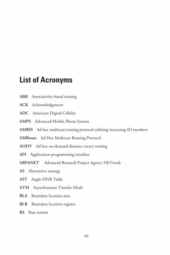
List of Acronyms

ABR Associativity-based routing

ACK Acknowledgement

ADC American Digital Cellular

AMPS Advanced Mobile Phone System

AMRIS Ad hoc multicast routing protocol utilizing increasing ID numbers

AMRoute Ad Hoc Multicast Routing Protocol

AODV Ad hoc on-demand distance vector routing

API Application-programming interface

ARPANET Advanced Research Project Agency NETwork

AS Alternative strategy

AST Angle-SINR Table

ATM Asynchronous Transfer Mode

BLA Boundary location area

BLR Boundary location register

BS Base station

195

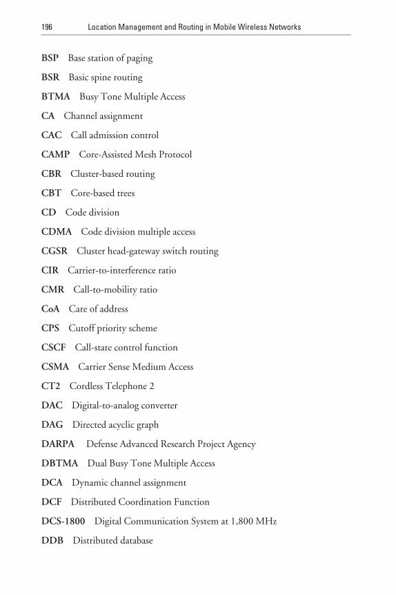
BSP Base station of paging

BSR Basic spine routing

BTMA Busy Tone Multiple Access

CA Channel assignment

CAC Call admission control

CAMP Core-Assisted Mesh Protocol

CBR Cluster-based routing

CBT Core-based trees

CD Code division

CDMA Code division multiple access

CGSR Cluster head-gateway switch routing

CIR Carrier-to-interference ratio

CMR Call-to-mobility ratio

CoA Care of address

CPS Cutoff priority scheme

CSCF Call-state control function

CSMA Carrier Sense Medium Access

CT2 Cordless Telephone 2

DAC Digital-to-analog converter

DAG Directed acyclic graph

DARPA Defense Advanced Research Project Agency

DBTMA Dual Busy Tone Multiple Access

DCA Dynamic channel assignment

DCF Distributed Coordination Function

DCS-1800 Digital Communication System at 1,800 MHz

DDB Distributed database


DECT Digital European Cordless Telephone

D-MAC Directional medium access control

DSDV Destination-sequenced distance vector routing protocol

DSR Dynamic source routing

DVMRP Distance vector multicast routing protocol

DVR Distance vector routing

EIA/TIA Electronics and Telecommunications Industry Associations

ESPAR Electronically steerable passive array radiator

ETSI European Telecommunication Standardization Institute

FAMA Floor Acquisition Multiple Access

FCA Fixed channel assignment

FD Frequency division

FDMA Frequency division multiple access

FGMP Forwarding Group Multicast Protocol

FPLMTS Future public land mobile telecommunications services

FSR Fisheye state routing

GHA Greedy Heuristic Algorithm

GPS Global positioning system

GRPS General Radio Packet Switching

GSM Global System for Mobile Communication

GTT Global title translation

HCA Hybrid channel assignment

HCS Hierarchical cellular system

HLR Home location register

HPCS Heterogeneous PCS

HSR Hierarchical spine routing


HSS Home subscriber service

IMS IP-based multimedia subsystem

IMT-2000 International Mobile Telecommunications 2000

IR Infrared

IS Interim standard

ISM Industrial, scientific, and medical

ITU International Telecommunication Union

LA Location area

LAR Location-aided routing

LILT Local information link-state topology

LINT Local information no topology

LLC Least cluster head change algorithm

LP-DDCA Locally packing distributed DCA

LOS Line of sight

LSP Link-state packet

LSR Link-state routing

LU Location update

MAC Medium access control

MACA Multiple Access with Collision Avoidance

MACAW Media Access Protocol for Wireless LANs

MAP Mobile application part

MCBS Multiple channel bandwidth system

MCDS Minimum connected dominating set

ME Minimum energy

MG Media gateway

MH Minimum hop


MGCF Media gateway control function

MMoIP Multimedia over IP

MOSPF Multicast open shorted path first

MPR Multipoint relay

MSC Mobile switching center

MS Mobile station

MT Mobile terminal

MU Mobile user

NGN Next-generation network

NLST Neighborhood-Link-State Table

ODMRP On-demand multicast routing protocol

OLSR Optimized link-state routing

OSPF Open Shortest Path First

PA Paging area

PACS Personal access communication systems

PCMA Power-Controlled MAC Protocol

PCSN Personal communication services network

PDC Personal Digital Cellular

PDE Partial differential equation

PDF Probability distribution function

PEDCP Path evaluation and data communication protocol

PFP Path finding protocol

PHS Personal handy phone system

PHY Physical

PIM Protocol independent multicast

PLMN Public land mobile network


PMAC Power-sensitive MAC protocol

PR Paging request

PSIP Parallel-to-sequential intelligent paging

PSTN Public switched telephone network

QoS Quality of service

RD Relative distance

RDM Relative distance microdiscovery

RDMAR Relative distance microdiscovery ad hoc routing

RF Radio frequency

RRA Resource allocation algorithm

RRM Radio resource management

RTS/CTS Request-to-send/clear-to-send

RUP Reuse partitioning

SDR Software-defined radio

SA Service area

SCP Signaling control point

SDC Start-of-data communication

SINR Signal-to-interference-and-noise ratio

SIP Sequential intelligent polling

SIR Signal-to-interference ratio

SNR Signal-to-noise ratio

SP Signaling point

SRMA Split-Channel Reservation Multiple Access

SSAR Signal stability-based adaptive routing

STP Signaling transfer point

TD Time division


TDMA Time division multiple access

TLDN Temporary local directory number

TORA Temporally-ordered routing algorithm

T-R Transmitter-receiver

TRCP Transmission range control protocol

TrFO Transcoder-free operation

TTM Time to migrate

UMTS Universal mobile telecommunication systems

VHE Virtual home environment

VLR Visitor location register

VoIP Voice over IP

WCDMA Wideband code division multiple access

WLAN Wireless local-area network

WPAN Wireless personal area network

WPBX Wireless private branch exchange

WRC World Radiocommunication Conference

WRP Wireless routing protocol

ZRP Zone routing protocol


.

TEAMFLY

Team-Fly®

About the Authors

Amitava Mukherjee has been a principal consultant of IBM Business Consult-ing Services, part of IBM Global Services (formerly PwC Consulting) in Cal-cutta, India, since 1995. He received his Ph.D. in computer science fromJadavpur University, Calcutta, India. He was with the Department of Electron-ics and Telecommunication Engineering at Jadavpur University, Calcutta,India, from 1983 to 1995. His research interests are in the area of mobile com-puting and communication, pervasive computing and M-commerce, opticalnetworks, combinatorial optimization, and distributed systems. His interestsalso include the mathematical modeling and its applications in the fields ofsocietal engineering and international relations. He is the author of over 65technical papers, one monograph, and four books. He is a member of IEEE andthe IEEE Communication Society.

Somprakash Bandyopadhyay is an associate professor with the MIS and Com-puter Science Group of the Indian Institute of Management, Calcutta. Prior tothat, he was in charge of the Knowledge Management and Learning & Profes-sional Development Group at PricewaterhouseCoopers Limited, a global man-agement consultancy firm in Calcutta for 6 years. Besides this industrialexperience, Dr. Bandyopadhyay has more than 15 years of experience in teach-ing, research, and software development at the Indian Institute of Technology,Kharagpur; the Indian Institute of Technology, Bombay; the Indian Institute ofManagement, Calcutta, Tata Institute of Fundamental Research, Bombay; andJadavpur University, Calcutta. He has a Ph.D. in computer science fromJadavpur University (1985) and a B.Tech. in electronics and electrical commu-nication engineering from the Indian Institute of Technology, Kharagpur

203

(1979). He was a fellow of the Japan Trust International Foundation andworked at the Advanced Telecommunication Research Institute in Kyoto,Japan, for 8 months in 2001, in the area of ad hoc wireless networks. He wasalso a fellow of the Alexander von Humboldt Foundation, Germany, and wasinvolved in postdoctoral research at the German Research Center for ArtificialIntelligence, Saarbrucken, for a year in 1989–1990.

Debashis Saha is currently an associate professor with the MIS and ComputerScience Group of the Indian Institute of Management, Calcutta, India. Hereceived his B.E. in electronics and telecommunication engineering. fromJadavpur University, Calcutta, India, in 1986, and his M.Tech. and Ph.D., bothin electronics and electrical communication engineering, from the Indian Insti-tute of Technology (IIT) at Kharagpur, India, in 1988 and 1996, respectively.He was a senior research scholar at IIT, Kharagpur, between 1988 and 1990,while conducting research on protocol engineering. He was with Jadavpur Uni-versity as a faculty member in the Computer Science & Engineering. Depart-ment from 1990 to 2001. His research areas are network protocols, WDMoptical networks, wireless and mobile communication and networking, and per-vasive computing. He has published more than 100 papers in various confer-ences and journals and delivered several invited talks and tutorials in networkingconferences and workshops. He is currently the principal investigator of twomajor funded projects on WDM optical networking research initiatives. He hascoauthored four books and a monograph. Dr. Saha is a life-member of theComputer Society of India (CSI), a member of IFIP WG 6.8, a Senior Memberof IEEE, and a member of the IEEE Computer Society and IEEE Communica-tion Society. He is a recipient of the prestigious Career Award for Young Teach-ers (1997) from the All India Council for Technical Education (AICTE),Government of India, and is a SERC visiting fellow (1999) and a BOYSCASTfellow (2000) of the Department of Science and Technology (DST), Govern-ment of India.


Index

3G systems, 1–2, 3, 4defined, 1mobility in, 26–29proposed standards, 2support, 3–4

Active routing, 187–88Adaptive transmission range control,

162–63Ad Hoc Multicast Routing Protocol

(AMRoute), 166–67defined, 166performance comparison, 170signaling component, 166simulation, 167See also Multicast routing protocols

Ad hoc multicast routing protocolutilizing increasing ID numbers(AMRIS), 167

Ad Hoc On-Demand Distance Vector(AODV), 143–44

defined, 143DSR vs., 168–70sequence numbers, 143–44specification, 144timer-based states maintenance, 144See also Reactive routing

Ad hoc wireless networks, 10–11, 115–71asymmetric link characteristics, 117bandwidth-constrained variable-capacity

links, 118

characteristics, 117–18clustered architecture, 119decentralized operation, 118defined, 10design choices, 118–23dynamics, 193dynamic topologies, 117energy-constrained operation, 118flat vs. hierarchical architecture, 119–20MAC protocol, 121–23MAC techniques, 125–33multicast routing protocols in, 165–68multihop communication, 117–18overview, 117–23performance comparisons, 168–70proactive vs. reactive routing, 120–21routing protocols, 135–71structure, 11topology control in, 159–61transmission power control in, 158–59

Advanced Mobile Phone System(AMPS), 54

All-IP networks, 179–81CSCF, 181drivers, 180evolution, 179–80HSS, 181illustrated, 181MG, 181MGCF, 181

205

ALOHA, 125–26defined, 125slotted, 125–26, 129

American Digital Cellular (ADC), 7Angle-SINR Table (AST), 130, 131Antennas

directional, 128–32ESPAR, 130omnidirectional, 125–28

Area zone model, 27–28Associativity-based routing (ABR), 145–46

advantages/drawbacks, 146defined, 145query packets, 146See also Reactive routing protocols

Automatic location management, 91

Base stations (BSs), 8, 31, 36antennas, 31fixed, 10multiple, 9number requirement, 43of paging (BSPs), 78

Basic spine routing (BSR), 164Blanket paging, 75–77Boundary LAs (BLAs), 87, 88Boundary location registers (BLRs), 87–88Busy Tone Multiple Access

(BTMA), 125, 126

Call admission control (CAC), 56–58algorithm, 56balancing power control, 57decisions, 58defined, 56generic function blocks of, 56interference-based, 57user-based, 57

Call state control function (CSCF), 181Call-to-mobility ratios (CMRs), 97, 107Care of address (CoA), 95–96Carrier Sense Medium Access

(CSMA), 125, 126collision avoidance (CSMA/CA), 132defined, 126See also Medium access control

(MAC) protocolsCarrier-to-interference ratio (CIR), 32

measurement DCA schemes, 51minimum level, maximizing, 51

Cell partitioning, 60–61MCBS, 60–61RUP, 60See also Radio resource management

(RRM)Cellular networks, 6–10

4G, 94architecture, 8–9, 193centralized entities, 15as infrastructured network, 3medium access, 9–10standards, 7–8

Centralized DCA, 51Channel allocation, 46–47Channel assignment (CA

algorithms, 50dynamic (DCA), 47fixed (FCA), 46–47hybrid (HCA), 47problem, 46schemes, 47–50

Channel borrowing schemes, 49City area model, 26–27

area zones, 26examples, 26illustrated, 27See also Metropolitan mobility

Cluster-Based Routing (CBR), 140Cluster Head-Gateway Switch Routing

(CGSR), 141Cochannel interference, 65–66Code division multiple access (CDMA),

9, 66–67advantages, 9–10soft handoff and, 53–54

Code division multiple access (Continued)systems, 67use of, 13wideband (WCDMA), 66See also Time division multiple access

(TDMA)Cognitive radio, 63Content-based routing, 187Cordless Telephone 2 (CT2), 7Core-Assisted Mesh Protocol

(CAMP), 167, 170Core-based trees (CBT), 165Correlation, 33Cutoff priority scheme (CPS), 55


Data-centric routing, 185–86Destination-Sequenced Distance VectorRouting Protocol (DSDV), 138–39

advantages, 139defined, 138routing updates, 138See also Proactive routing protocols

Diffraction, 34Diffusion model, 22Digital Communication System 1800

(DCS1800), 7Digital European Cordless Telephone

(DECT), 7Digital to analog converter (DAC), 62Directed acyclic graph (DAG), 144–45Directional antennas, 128–32Distance Vector Multicast Routing

Protocol (DVMRP), 165Distance vector routing (DVR) protocols,

135–36, 171Distributed Coordination Function (DCF),

127Distributed DCA, 51Distributed wireless sensor networks,

182–86introduction, 182postdeployment phase, 184predeployment and deployment phase,

184redeployment of additional nodes phase,

184routing, 184–86sensor deployment, 183–84topology maintenance, 183–84

Dual Busy Tone Multiple Access(DBTMA), 125, 127–28

Dynamic channel assignment(DCA), 50, 66

centralized, 51CIR measurement, 51defined, 47distributed, 51gains, 52one dimension systems, 51schemes, 50strategies, 47–48See also Channel assignment (CA)

Dynamic source routing (DSR), 142–43advantages, 143

AODV vs., 168–70defined, 142drawbacks, 143See also Reactive routing protocols

Electronically steerable passive arrayradiator (ESPAR), 130

Electronics and TelecommunicationsIndustry Associations(EIA/TIA), 90

Exposed terminal problem, 122

Federal Communications Commission(FCC), 38, 40

functions, 38TV Band management, 40

First-generation systems, 2First in-first out (FIFO), 58Fisheye State Routing (FSR), 141–42

defined, 141“fisheye” technique, 141link-state packets, 142multilevel fisheye scope, 142See also Proactive routing protocols

Fixed channel assignment (FCA), 48–49defined, 46–47schemes, 47

Fixed channel assignment (Continued)strategy, 48–49See also Channel assignment (CA)

Flat architecture, 119–20Flooding, 186Floor Acquisition Multiple Access

(FAMA), 125, 128Fluid flow model, 18–22

accuracy, 18defined, 18oneway highway streets, 19time-homogeneous deterministic,

21–22time-nonhomogeneous deterministic,

19–21See also Mobility modelsForwarding Group Multicast Protocol

(FGMP), 166Frequency division multiple access

(FDMA), 9

General Packet Radio Switching(GPRS), 73–74

Index 207

Global System for Mobile Communication(GSM), 7

frequencies, 41interconnected networks, 91mobile application part (MAP), 90terminals, 41

Global title translation (GTT), 76Gossiping, 186Granularity factor, 77Gravity model, 22–23

advantage, 23defined, 22See also Mobility models

Greedy Heuristic Algorithm (GHA),100–101

defined, 105description of, 105–7pseudocode, 105–6

Guard channel concept, 55

Handoffcost, 104hard, 52–53prioritization schemes, 55process, 52–55soft, 53–55

Hard handoff, 52–53defined, 52intercell, 52–53intracell, 52scenario, 53See also Handoff

Hidden terminal problem, 122Hierarchical ad hoc networks, 119–20

advantages, 120illustrated, 119nodes, 119See also Ad hoc wireless networks

Hierarchical cellular systems (HCS), 59Hierarchical spine routing (HSR), 164Home location register (HLR), 8, 73, 74Home subscriber server (HSS), 181Hybrid channel assignment (HCA), 47, 48

IEEE 802.11, 127IMT-2000 systems, 6, 66

core-band spectrum, 41–42extension bands, 42–43terrestrial services, 42

Indoor wireless, 37

Instantaneous capacity, 45Intelligent paging, 78–84

algorithm, 79parallel-o-sequential (PSIP), 80, 82–83sequential, 81–82strategy, 79See also Paging

International allocations, 38–39International mobility model, 29International Telecommunications Union

(ITU), 38–39primary/secondary allocation

designation, 38–39Radio Regulations, 42

Intersystem paging, 87–88IS-41, 90

LA planning, 97–109cell area is equal to LA, 108–9GHA description, 105–7LU cost, 102methodology, 99–101optimization of LMCF, 103paging cost, 101–2proposed architecture, 97–99signal requirements and, 107–9solution techniques, 101–7system area is equal to LA, 108total recurring system cost, 102two-step approach, 97–107See also Location areas (LAs)

Link-state routing (LSR) protocols,136, 171

Local information link-state topology(LILT), 160

Local information no topology(LINT), 160–61

Location-Aided Routing (LAR) protocols,152–53

defined, 152routing failure detection, 153See also Reactive routing protocols

Location areas (LAs), 70boundary (BLA), 87, 88crossing, 71defined, 70dynamic strategy, 72multilayer, 92number of PAs within, 75PAs combination with, 92


planning, 97–109size of, 92–93static strategy, 72

Location-based multicast scheme, 168Location management, 11–13, 69–109

automatic, using LA, 91basis, 89as key factor, 109manual registration in, 90memory-based, 92–93memoryless-based, 91–92mobility models, 12–13in next-generation systems, 93–96radio resource management, 13standards, 90tasks, 11–12techniques, 12tracking, 13without, 90See also Location update; Paging

Location tracking, 13defined, 13–14end point differentiation, 14

Location update, 11–12, 69, 71–74cost, 102defined, 71dynamic strategies, 72–74static strategies, 72strategies, 71–74See also Location management

Markov chain, 24, 25Markov walk model, 23, 24Media gateway control function

(MGCF), 181Media gateway (MG), 181Medium access control (MAC) protocols,

121–23ALOHA, 125–26, 129BTMA, 125, 126collision avoidance capability, 121CSMA, 125, 126CSMA/CA, 132DBTMA, 125, 127–28development, 123with directional antennas, 128–32directional (D-MAC), 129ESPAR, 130FAMA, 125, 128

MACA, 125, 126, 128MACAW, 125, 126, 128with omnidirectional antennas, 125–28power-controlled (PCMAs), 158–59purpose, 123techniques, 125–33

Medium Access Protocol for WirelessLANs (MACAW), 125, 126, 128

Memory-based location management,92–93

dynamic LA/PA size, 92–93individual user patterns, 93See also Location management

Memoryless-based location management,91–92

database architecture, 91fixed network architecture optimization,

91–92LAs/PAs combination, 92

multilayer LAs, 92See also Location management

Metropolitan mobility, 26–28area zone model, 27–28city area model, 26–27street unit model, 28See also Mobility; Mobility models

Minimum connected dominating set(MCDS), 164

Mobile agent-based protocol, 154–58framework, 154–55mechanism, 155–56for topology discovery, 154–55uninterrupted connection management,

156–58See also Routing protocolsMobile-controlled handoff.

See Soft handoffMobile IP, 88–89

architecture, 96low-latency handover in, 89

Mobile stations (MSs), 12, 36Mobile switching center (MSCs), 8, 97Mobile terminals (MTs), 31, 36

in blanket paging, 75–77in intelligent paging, 78–84mobility, 45mobility model of, 99–100movement of, 52simulating movement of, 99

Index 209

Mobilityin 3G systems, 26–29issues, 17–29metropolitan, 26–28MTs, 45

Mobility Manager (MM), 80Mobility models, 12–13, 18–26

area zone model, 27–28city area model, 26–27diffusion model, 22fluid flow model, 18–22gravity model, 22–23international model, 29metropolitan model, 26–28of MTs, 99–100national model, 28–29random walk model, 23–26street unit model, 28types of, 18

Moore’s Law, 193Multicast open shorted path first

(MOSPF), 165Multicast routing protocols, 165–68

AMRIS, 167AMRoute, 166–67CAMP, 167CBT, 165DVMRP, 165FGMP, 166location-based, 168MOSPF, 165ODMRP, 167, 170performance comparisons, 168–70PIM, 165stability-based, 168See also Routing protocols

Multilayered architecture, 61Multipath

fading, 34routing, with preemptive route

discovery, 150–52Multiple Access with Collision Avoidance

(MACA), 125, 126, 128Multiple channel bandwidth system

(MCBS), 60–61

National mobility model, 28–29National Telecommunications and

Information Administration(NTIA), 38

Neighborhood-Link-State Table(NLST), 130

Network-controlled handoff.See Hard handoff

Omnidirectional antennas, 125–28On-Demand Multicast Routing

Protocol (ODMRP), 167, 170On-demand routing, 153–54Optimized Link-State Routing

(OLSR) protocol, 164Organization, this book, xvi–xvii

Paging, 11–12, 69, 75–89blanket, 75–77cost, 101–2cost comparison, 83–84defined, 75delay, 84–85efficient, 77intelligent scheme, 78–84intersystem, 87–88IP micromobility and, 88–89procedures, 77–78reverse, 85–86semireverse, 86triggers, 89uniform, 86worst-case delay, 84–85See also Location management

Paging areas (PAs), 70defined, 70LAs combination, 92number within LA, 75size of, 92–93

Parallel-o-sequential intelligent paging(PSIP), 80, 82–83

algorithm, 82–83defined, 82See also Intelligent paging

Partial differential equations(PDEs), 19, 20

Path Evaluation and Data CommunicationProtocol (PEDCP), 162

Path Finding Protocol (PFP), 162Path loss, 33–35

defined, 33formula, 34See also Radio propagation


Personal Access Communications Systems(PACS), 7

Personal communication services network(PCSN), 97

architecture, 98design, 107popularity, 99

Personal Communications System (PCS), 7Personal Digital Cellular (PDC), 7Personal Handy Phone System (PHS), 7Pervasive networks, 187, 191Pervasive routing, 186–88Power-aware routing protocols, 158–63with adaptive transmission range control,

162–63optimal transmission range, 161–62topology control, 159–61

transmission power control, 158–59See also Routing protocols

Power-controlled MAC protocols(PCMAs), 158–59, 162

Power-controlled multiple access, 132–33Primary allocations, 39Proactive routing protocols, 120–21

CBR, 140CGSR, 141DSDV, 138–39FSR, 141–42WRP, 139–40See also Routing protocols

Propagation. See Radio propagationProtocol independent multicast (PIM), 165

Quality of service (QoS), 55, 58–59end-to-end, 58management, 65overprovisioning, 64requirements, 58service support, 65user requirements, 56

Query localization, 153–54Queuing, 58

Radio propagation, 32–37correlation, 33free-space, 34indoor wireless, 37multipath components, 33path loss, 33–35reciprocity, 35–37

shadowing, 33, 35temporal fading, 33

Radio resource management(RRM), 13, 43–52

cell partitioning, 60–61channel allocation/assignment, 46–47emerging techniques, 60–63integrated model, 65integrating, 63–65multilayered architecture, 61problem, 43–46schemes, 43software radio, 61–63virtual access node, 64

Random walk model, 23–26defined, 23state diagram, 24See also Mobility models

Reactive routing protocols, 121, 142–54ABR, 145–46AODV, 143–44, 168–70defined, 137DSR, 142–43, 168–70LAR, 152–53multipath routing with preemptive

route discovery, 150–52query localization, 153–54SSAR, 146–47stability-based routing, 147–50TORA, 144–45, 169–70

Reciprocity, 35–37Relative Distance Microdiscovery Ad Hoc

Routing (RDMAR) protocol,164–65

Request-to-Send/Clear-to-Send(RTS/CTS), 126–28

basic mechanism, 127dialog, 127, 128handshaking mechanism, 126, 129

Resource allocation algorithm(RAA), 43, 45

Resource allocation management, 55–59CAC, 56–58

QoS, 58–59Reuse partitioning (RUP), 60Reverse paging, 85–86Route discovery, 135, 150–52Route maintenance, 135

Index 211

Routingactive, 187–88content-based, 187data-centric, 185–86in distributed wireless sensor networks,

184–86energy-efficient, 185pervasive, 186–88

Routing protocols, 13–15ABR, 145–46ad hoc wireless networks, 135–71AMRIS, 167AMRoute, 166–67AODV, 143–44, 168–70BSR, 154CAMP, 167CBR, 140CGSR, 141DSDV, 138–39DSR, 142–43, 168–70DVR, 135–36, 171FGMP, 166FSR, 141–42HSR, 154, 164LAR, 152–53LSR, 136, 171mobile agent-based, 154–58multipath routing with preemptive

route discovery, 150–52ODMRP, 167, 170OLSR, 164power-aware, 158–63proactive, 120–21, 138–42problem, 135query localization, 153–54RDMAR, 164–65reactive, 121, 137, 142–54SSAR, 146–47stability-based routing, 147–50TORA, 144–45, 169–70unicast, 138–65WRP, 139–40ZRP, 163

Seamless access, 193Secondary allocations, 39Second-generation systems, 2–3Semireverse paging, 86Sensor networks, 182–83

design challenges, 182

many-to-one data flows, 183stress levels, 186See also Distributed wireless sensor

networksSequential intelligent paging, 81–82Shadowing, 33, 35

boundary approximation geometry, 36defined, 33effects, 35See also Radio propagation

Signal Stability-Based Adaptive Routing(SSAR), 146–47

advantages/drawbacks, 147defined, 146query-reply process, 146See also Reactive routing protocols

Signal-to-interference ratio (SIR), 43, 44Signal-to-noise ratio (SNR), 32Slotted ALOHA, 125–26, 129Soft handoff, 53–55

benefits, 54defined, 53realization requirements, 54See also handoff

Software-defined ratio (SDR), 62Software radio, 61–63

channel modulation waveforms, 62cognitive radio, 63defined, 61–62SDR, 62use of, 62–63See also Radio resource management

(RRM)Spectrum

management financing, 39monitoring/enforcement, 39–41

Spectrum allocation, 38international, 38–39primary, 39secondary, 39

Split-Channel Reservation Multiple Access(SRMA), 126

Stability-based multicast scheme, 168Stability-based routing, 147–50

defined, 147–48example network illustration, 150link-affinity, 148, 149link stability, 148node-affinity, 149


TEAMFLY

Team-Fly®

path-searching mechanism, 149–50path stability, 148See also Reactive routing protocols

Street unit model, 28

Telegraphic theory, 44Teletraffic models, 18Temporal fading, 33Temporally Ordered Routing Algorithm(TORA), 144–45

defined, 144directed acyclic graph (DAG), 144–45multiple paths, 145performance comparison, 169–70See also Reactive routing protocols

Temporary location directory number(TLDN), 76

Third-generation systems. See 3G systemsTime division multiple access (TDMA), 9

advantages, 9–10soft handoff and, 53–54use of, 13See also Code division multiple access

(CDMA)Total recurring system cost, 102Traffic modeling, 100Traffic sessions, 14Transmission power

adjusting, 159–61control, 50–52, 158–59

Transmission rangeadaptive control, 162–63optimal, 161–62

Transmission Range Control Protocol(TRCP), 162

Two-step approach. See LA planning

Unicast routing protocols, 138–65mobile agent-based, 154–58performance comparisons, 168–70power-aware, 158–63proactive, 138–42reactive, 142–54See also Routing protocols

Uniform paging, 86Universal mobile telecommunications

system (UMTS), 7all-IP networks, 179–81wideband code division multiple access

(WCDMA), 7

Visitor location register (VLR), 8–9, 73,74, 91

Voice over IP (VoIP), 95

Wireless networks1G, 22G, 2–33G, 1–2ad hoc, 10–11, 115–71generations of, 2mobile, 5–6mobility support, 5routing techniques, 13–15, 135–71types of, 5

Wireless personal area networks(WPANs), 94

Wireless private branch exchange(WPBX), 1

Wireless Routing Protocol (WRP), 139–40

Zone Routing Protocol (ZRP), 163

Index 213

Documents

F L Y A M T E - SRIJAN (सृजन) TUTORIALS · 3.4.2 Mobile-Controlled Handoff (Soft Handoff) 53 3.4.3 Handoff Prioritizing Schemes 55 3.5 Managing Resource Allocation 55 3.5.1