Data Wrangling

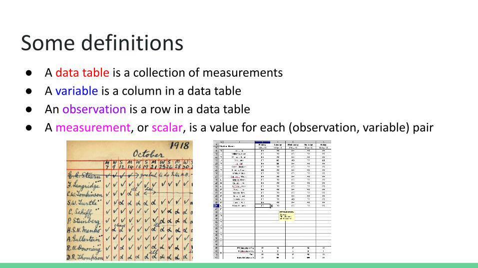
Some definitions● A data table is a collection of measurements

● A variable is a column in a data table

● An observation is a row in a data table

● A measurement, or scalar, is a value for each (observation, variable) pair

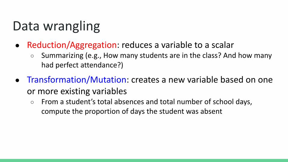
Data wrangling● Reduction/Aggregation: reduces a variable to a scalar

○ Summarizing (e.g., How many students are in the class? And how many had perfect attendance?)

● Transformation/Mutation: creates a new variable based on one or more existing variables○ From a student’s total absences and total number of school days,

compute the proportion of days the student was absent

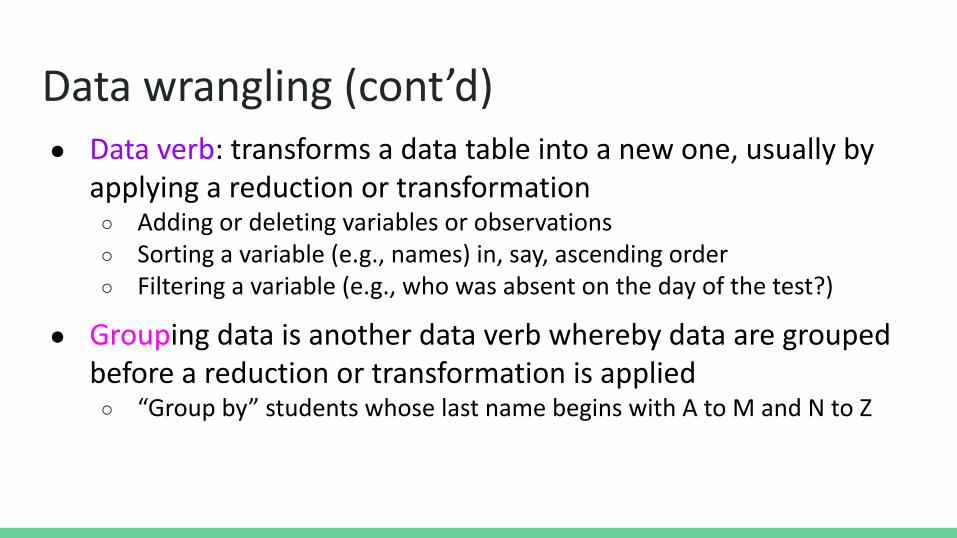
Data wrangling (cont’d)● Data verb: transforms a data table into a new one, usually by

applying a reduction or transformation○ Adding or deleting variables or observations○ Sorting a variable (e.g., names) in, say, ascending order○ Filtering a variable (e.g., who was absent on the day of the test?)

● Grouping data is another data verb whereby data are grouped before a reduction or transformation is applied○ “Group by” students whose last name begins with A to M and N to Z

dplyr

What is dplyr?● An R package full of data verbs

● Some examples of things it can do○ Select (variables)○ Filter (observations)○ Sort (rearrange data)○ Summarize (e.g., mean)○ Transform (e.g., add columns)○ The elusive group_by() operation

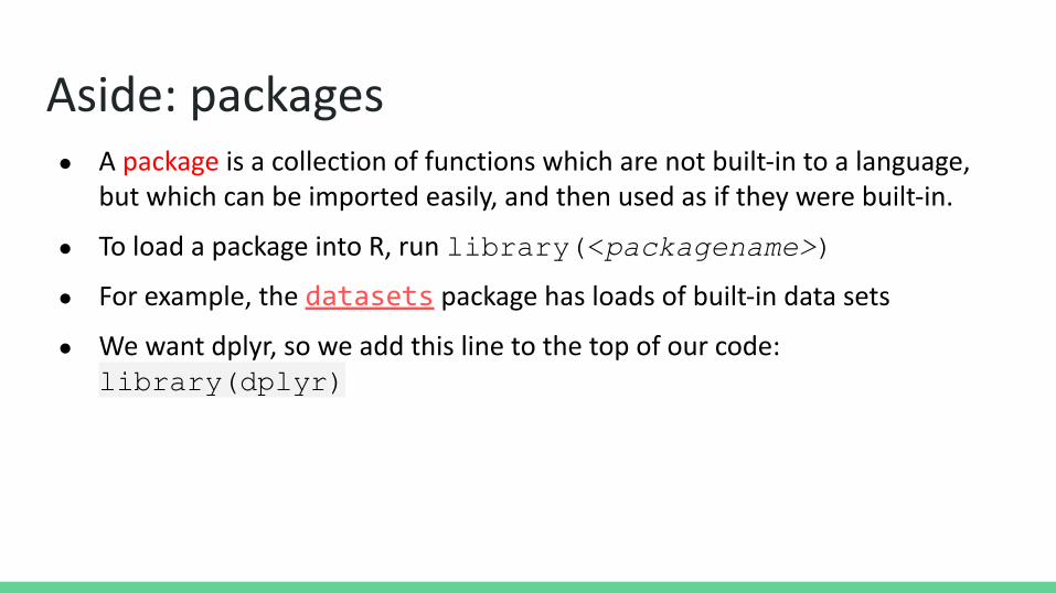
Aside: packages● A package is a collection of functions which are not built-in to a language,

but which can be imported easily, and then used as if they were built-in.

● To load a package into R, run library(<packagename>)

● For example, the datasets package has loads of built-in data sets

● We want dplyr, so we add this line to the top of our code: library(dplyr)

Our data: A survey sent to Slovakian youth in 2013

● The data set consists of responses to 150 questions, covering topics such as music/movie preferences, hobbies and interests, spending habits, etc.

● Contains 1010 rows and 150 columns

A sample of questions from the survey. Complete information is available here.

Sample survey questions

Column Name Question

Reliability I am reliable at work and always complete all tasks given to me.

Keeping promises I always keep my promises.

Loss of interest I can fall for someone very quickly and then completely lose interest.

Friends versus money I would rather have lots of friends than lots of money.

Funniness I always try to be the funniest one.

Fake I can be two faced sometimes.

Criminal damage I damaged things in the past when angry.

Decision making I take my time making decisions.

Empathy I am an empathetic person.

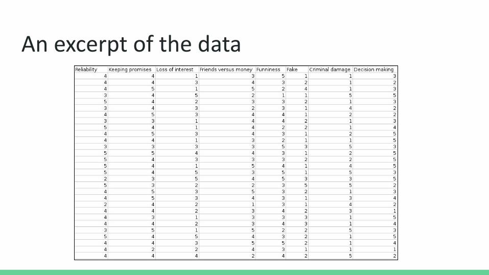
An excerpt of the data

To store the data set in a data frame called responses:

responses <- read.table("~/R/dplyr/responses.csv", sep = ";", header = TRUE)

To see the head, or the first six rows, of responses:

head(responses)

Importing data into RStudio

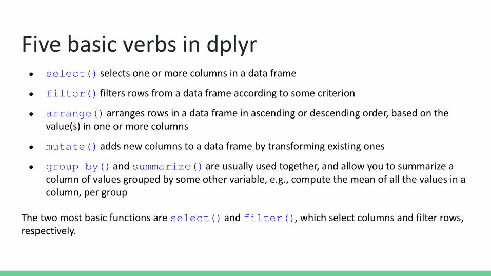
Five basic verbs in dplyr● select() selects one or more columns in a data frame

● filter() filters rows from a data frame according to some criterion

● arrange() arranges rows in a data frame in ascending or descending order, based on the value(s) in one or more columns

● mutate() adds new columns to a data frame by transforming existing ones

● group_by() and summarize() are usually used together, and allow you to summarize a column of values grouped by some other variable, e.g., compute the mean of all the values in a column, per group

The two most basic functions are select() and filter(), which select columns and filter rows, respectively.

Selecting columns with select()We can select columns by listing their names explicitly: age, gender, and education

head(select(responses, Age, Gender, Education))

And we can select a range of columns using the ‘:’ operator:

head(select(responses, Reliability:Decision.making))

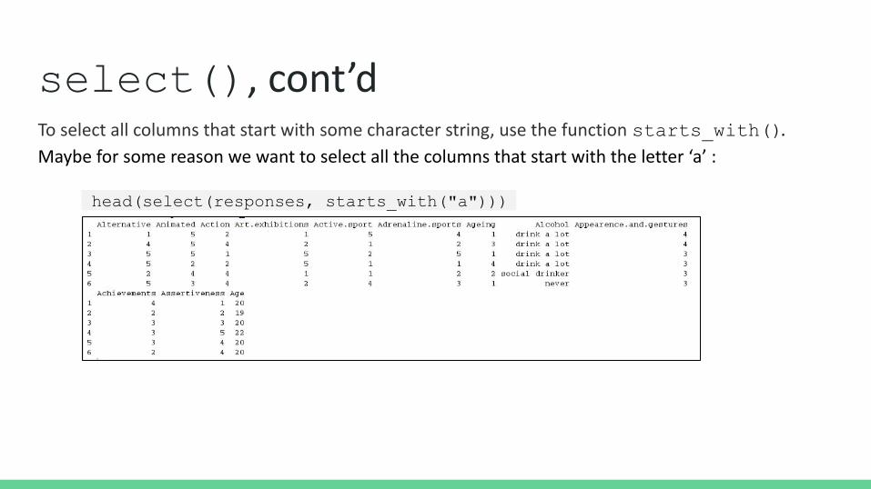
To select all columns that start with some character string, use the function starts_with().

Maybe for some reason we want to select all the columns that start with the letter ‘a’ :

head(select(responses, starts_with("a")))

select(), cont’d

select(), cont.Some additional options to select columns based on a specific criteria include:

1. ends_with() Select columns that end with a character string

2. contains() Select columns that contain a character string

3. matches() Select columns that match a regular expression

4. one_of() Select columns names that are from a group of names

Selecting rows with filter()Filter the rows for young people who consider themselves empathetic:

head(filter(responses, Empathy > 3))

Some potentially interesting findings here: These individuals skew towards agreement with the statement “I find it very difficult to get up in the morning.” All of them responded neutrally to the statement “I believe all my personality traits are positive.” And, ⅚ of them are female. (Of course, these are only the first 6 individuals who consider themselves empathetic.)

filter(), cont’dFilter for young people who consider themselves empathetic and feel lonely in life:

head(filter(responses, Empathy > 3, Loneliness > 3))

They mostly consider themselves procrastinators, would rather have friends than money, and would change the past if they could.

filter(), cont’dFilter for people who are under the age of 20, enjoy meeting new people, and drink alcohol:

head(filter(responses, Age < 20, Socializing > 3, Alcohol %in% c("social drinker", "drink a lot")))

They aren’t so interested in Western movies, writing, or gardening; but they like comedies, romantic movies, and foreign languages.

%>%, cont’dRecall how to select:

head(select(responses, Age, Gender, Education))

Here it is again, using piping:

responses %>%select(Age, Gender, Education) %>% head

We are piping the responses data frame to

the select() function to extract the three

columns (age, gender, and education), and then

we are piping the ensuing data frame to the

head() function.

● The pipe operator allows you to pipe the output from one function to the input of another function

● Instead of nesting functions as we’ve been doing (reading from the inside to the outside), the idea of of piping is to read the functions from left to right

Pipe operator: %>%

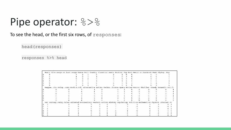
To see the head, or the first six rows, of responses:

head(responses)

responses %>% head

Pipe operator: %>%

Arrange rows with arrange()To arrange rows by the values in a particular column or columns, use the arrange() function,

with the name(s) of the column(s) you want to arrange the rows by as argument(s):

responses %>% arrange(Age) %>% head

Taking the head of the data frame arranged by age yields the responses of six 15-year-olds, who aren’t super

likely to spend their money on healthy eating, and prefer branded clothing to non-branded.

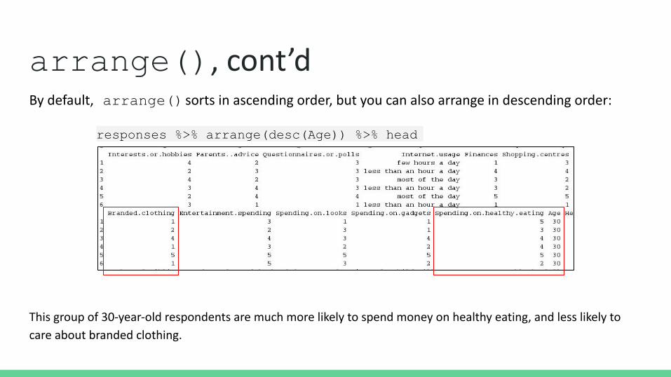
arrange(), cont’dBy default, arrange() sorts in ascending order, but you can also arrange in descending order:

responses %>% arrange(desc(Age)) %>% head

This group of 30-year-old respondents are much more likely to spend money on healthy eating, and less likely to

care about branded clothing.

● The real power of piping is that it enables us to seamlessly combine dplyr data verbs

Pipe operator: %>%

arrange(), cont’dLet’s select a few columns and arrange the rows by number of friends:

responses %>% select(Age, Gender, Number.of.friends, Happiness.in.life) %>% arrange(Number.of.friends) %>% head

Again, in descending order:

responses %>% select(Age, Gender, Number.of.friends, Happiness.in.life) %>% arrange(desc(Number.of.friends)) %>% head

(Note the correlation between number of friends and happiness in life.)

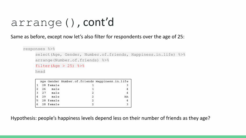
arrange(), cont’dSame as before, except now let’s also filter for respondents over the age of 25:

responses %>% select(Age, Gender, Number.of.friends, Happiness.in.life) %>% arrange(Number.of.friends) %>%filter(Age > 25) %>% head

Hypothesis: people’s happiness levels depend less on their number of friends as they age?

Create new columns using mutate()The mutate() function adds new columns to a data frame. Let’s create a new column called

decision_regrets, which will be the ratio of responses to the statement

“I take my time to make decisions” to “I often think about and regret the decisions I make”:

responses %>% mutate(decision_regrets = Decision.making / Self.criticism) %>% select(Age, decision_regrets) %>% head

Note the selection for Age and the new decision_regrets columns.

Otherwise, the new data frame would contain all 150 columns.

Create summaries using summarise()The summarise() function creates a new data frame that summaries a column in the given data frame. For example, to compute the

mean happiness, apply the mean() function to the column Happiness.in.life and call the value avg_happiness.

(Because some survey respondents left this field blank, we remove the N/A responses using filter() and !is.na.)

responses %>% summarise(avg_happiness = mean(Happiness.in.life))

responses %>% summarise(avg_happiness = mean(Happiness.in.life, na.rm = TRUE))

Create summaries using summarise()If we want to compare the average happiness of female vs. male respondents, we can also filter by gender:

responses %>% filter(Gender == "female") %>%

summarise(avg_happiness = mean(Happiness.in.life, na.rm = TRUE))

responses %>% filter(Gender == "male") %>%

summarise(avg_happiness = mean(Happiness.in.life, na.rm = TRUE))

summarise(), cont’dThere are many other summary statistics, such as:● sd() ● min() ● max() ● median() ● sum()● n() (the length of a column)

● first() (the first value in a column)

● last() (the last value in a column)

● n_distinct() (the number of distinct values in a column)

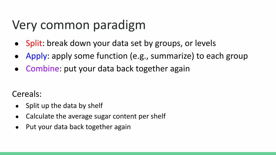
Very common paradigm● Split: break down your data set by groups, or levels

● Apply: apply some function (e.g., summarize) to each group

● Combine: put your data back together again

Cereals:● Split up the data by shelf

● Calculate the average sugar content per shelf

● Put your data back together again

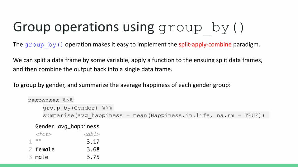
Group operations using group_by()The group_by() operation makes it easy to implement the split-apply-combine paradigm.

We can split a data frame by some variable, apply a function to the ensuing split data frames,

and then combine the output back into a single data frame.

To group by gender, and summarize the average happiness of each gender group:

responses %>% group_by(Gender) %>% summarise(avg_happiness = mean(Happiness.in.life, na.rm = TRUE))

group_by(), cont.Now, combining functions, we can split the data frame by age, gender, number of siblings, or any

other “factor”, and then ask for the average scores to the following questions, from left to right:

1. I am 100% happy with my life.

2. I live a very healthy lifestyle.

3. I look at things from all different angles before I go ahead.

4. I always try to vote in elections.

5. I am not afraid to give my opinion if I feel strongly about something.

6. I feel lonely in life.

7. I spend a lot of money on my appearance.

This gives us a set of summary statistics grouped by age.

The rightmost column reports the total number of respondents by age.

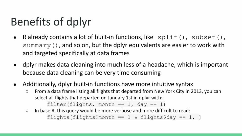
Benefits of dplyr ● R already contains a lot of built-in functions, like split(), subset(),

summary(), and so on, but the dplyr equivalents are easier to work with and targeted specifically at data frames

● dplyr makes data cleaning into much less of a headache, which is important because data cleaning can be very time consuming

● Additionally, dplyr built-in functions have more intuitive syntax○ From a data frame listing all flights that departed from New York City in 2013, you can

select all flights that departed on January 1st in dplyr with: filter(flights, month == 1, day == 1)

○ In base R, this query would be more verbose and more difficult to read: flights[flights$month == 1 & flights$day == 1, ]