Embed Size (px)
Citation preview
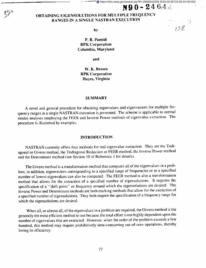
.)f OBTAINING EIGENSOLUTIONS FOR MULTIPLE FREQUENCY
RANGES IN A SINGLE NASTRAN EXECUTION
by
P. R. Pamidi
RPK Corporation
Columbia, Maryland
and
W. K. Brown
RPK Corporation
Hayes, Virginia
SUMMARY
A novel and general procedure for obtaining eigenvalues and eigenvectors for multiple fre-
quency ranges in a single NASTRAN execution is presented. The scheme is applicable to normal
modes analyses employing the FEER and Inverse Power methods of eigenvalue extraction. The
procedure is illustrated by examples.
INTRODUCTION
NASTRAN currently offers four methods for real eigenvalue extraction. They are the Tridi-
agonal or Givens method, the Tridiagonal Reduction or FEER method, the Inverse Power method
and the Determinant method (see Section 10 of Reference 1 for details).
The Givens method is a transformation method that computes all of the eigenvalues in a prob-
lem; in addition, eigenvectors corresponding to a specified range of frequencies or to a specified
number of lowest eigenvalues can also be computed. The FEER method is also a transformation
method that allows for the extraction of a specified number of eigensolutions. It requires the
specification of a "shift point" or frequency around which the eigensolutions are desired. The
Inverse Power and Determinant methods are both tracking methods that allow for the extraction of
a specified number of eigensolutions. They both require the specification of a frequency range for
which the eigensolutions are desired.
When all, or almost all, of the eigenvalues in a problem are required, the Givens method is the
generally the most efficient method to use because the total effort is not highly dependent upon the
number of eigenvalues that are extracted. However, when the order of the problem exceeds a few
hundred, this method may require prohibitively time-consuming out-of-core operations, thereby
losing its efficiency.
77
https://ntrs.nasa.gov/search.jsp?R=19900015328 2019-03-05T22:06:22+00:00Z
If an user is not interested in obtaining all of the modes in a problem, but only in a smaller
number of eigensolutions around a certain frequency or within a certain frequency range, the FEER,
the Inverse Power and the Determinant methods are the obvious choices. The computations in all
of these methods are proportional to the number of eigensolutions extracted. The FEER method is
probably the most efficient of the three. It is quite effective in obtaining eigensolutions around the
selected frequency. It is also very efficient even when out-of-core operations are involved. The
results obtained by the Inverse Power and Determinant methods, on the other hand, are very
susceptible to the number of estimated roots specified for a given frequency range (field 5 on the
EIGR bulk data card; see Reference 2). When the specified number for the estimated roots is larger
than the actual number of roots in that range, these methods are apt to yield many lower frequencies
outside the specified frequency range. The Determinant method is the least efficient of all of the
methods and will, therefore, not be considered any further for the purpose of this paper.
CURRENT PROCEDURE FOR OBTAINING EIGENSOLUTIONS
FOR MULTIPLE FREQUENCY RANGES
There are practical situations in which an user may be interested in obtaining eigensolutions for
multiple frequency ranges, with one frequency range quite distinct and apart from another frequency
range. Complex configurations involving control systems, experimental setups and structural
subsystems are examples of such situations.
None of the eigenvalue extraction methods discussed earlier can accomplish the above objec-
tive directly. So, if the user wishes to obtain eigenvalues for more than one range of frequencies in
such cases as the above, he can accomplish it at present in one of two ways. The first way is for the
user to make a single NASTRAN execution with a large frequency range (or a shift point in
conjunction with a large number of desired roots) so as to encompass all of the frequencies in the
ranges of interest. However, this will not be very cost effective if the frequency ranges of interest
are widely separated. The alternative way is for the user to perform multiple NASTRAN executions,
one execution for each range of frequencies, effectively utilizing the APPEND feature (see Section
9.2.2 in Reference 1 and Section 2.3.7 in Volume 2, Reference 2). However, this latter procedure
involves checkpoint/restart runs and is rather cumbersome for the purpose.
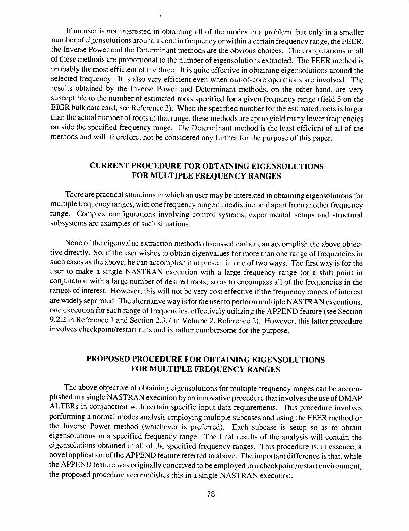
PROPOSED PROCEDURE FOR OBTAINING EIGENSOLUTIONS
FOR MULTIPLE FREQUENCY RANGES
The above objective of obtaining eigensolutions for multiple frequency ranges can be accom-
plished in a single NASTRAN execution by an innovative procedure that involves the use of DMAP
ALTERs in conjunction with certain specific input data requirements. This procedure involves
performing a normal modes analysis employing multiple subcases and using the FEER method or
the Inverse Power method (whichever is preferred). Each subcase is setup so as to obtain
eigensolutions in a specified frequency range. The final results of the analysis will contain the
eigensolutions obtained in all of the specified frequency ranges. This procedure is, in essence, a
novel application of the APPEND feature referred to above. The important difference is that, while
the APPEND feature was originally conceived to be employed in a checkpoint/restart environment,
the proposed procedure accomplishes this in a single NASTRAN execution.
78
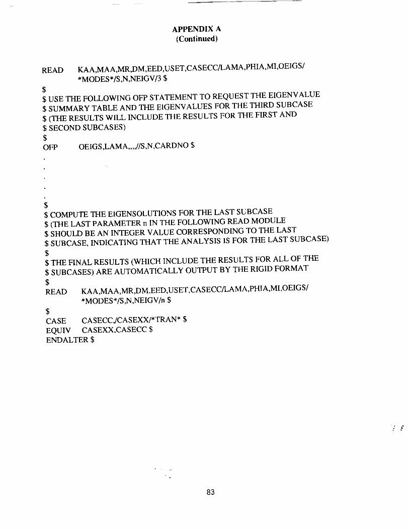
The DMAP ALTER package required for the above procedure is given in Appendix A. The
details of the input data requirements and the output obtained from the analysis are discussed below.
Executive Control Deck
The user should employ the DMAP ALTER package given in Appendix A either by explicitly
including it or by referencing it via a READFILE card in the Executive Control Deck. Note that,
for every additional subcase beyond the first subcase, the ALTER package involves a pair of OFP
and READ modules.
Case Control Deck
The user should have as many subcases in the Case Control Deck as the number of distinct
frequency ranges for which he wishes to obtain eigensolutions. Each subcase must have a separate
METHOD request. The METHOD request in each subcase references a distinct EIGR card in the
Bulk Data Deck that either implies (in the case of the FEER method) or defines (in the case of the
Inverse Power method) a distinct frequency range.
All output requests and constraint specifications must be above the subcase level. Thus, the only
difference between one subcase and another must be the different METHOD that they request. Also,
since the final results include eigensolutions for all of the subcases, PLOT requests should not make
explicit references to subease numbers.
Bulk Data Deck
In addition to the required modeling (geometry, constraints, etc.) data, the Bulk Data Deck
should have as many EIGR cards as the number of subcases employed (and the corresponding
METHOD requests) in the Case Control setup.
When using the FEER method, the EIGR bulk data card for each METHOD request requires
the specification of a shift point or frequency that indicates the center of a frequency range as well
as the number of desired roots (see Reference 2). The user should specify appropriate values
accordingly. The shift point specified has a significant effect on the actual eigensolutions extracted.
Accordingly, depending upon the shift point specified, the actual number of roots computed may be
more or less than the number of desired roots specified in the data.
When using the Inverse Power method, the EIGR bulk data card for each METHOD request
requires the specification of a frequency range, the number of desired roots as well as the number
of estimated roots in the specified frequency range (see Reference 2). The number of estimated roots
specified has a significant effect on the actual eigensolutions extracted. However, the user, in
general, will not have an a priori idea of the actual number of eigenvalues that may exist in a
particular frequency range. Accordingly, the user should use his best judgment to specify this
number. A number for the estimated roots that is larger than the actual number of roots in that range
will, in general, yield a number of lower frequencies that are outside the specified frequency range.
It should also be noted here the eigensolutions resulting from any particular subcase will include
not only the eigensolutions that are computed in that subcase, but also the eigensolutions resulting
79
from all previoussubcases.Accordingly,regardlessof which eigenvalueextractionmethodisemployed,thenumberof desiredrootsspecifiedon theEIGRcard for a particularsubcasemustallownotonlyfortherootsthatwill becomputedbythatsubcase,butalsoincludetherootscomputedby all of theprevioussubcases.
Output from the Analysis
As mentioned earlier, the final results from the analysis will include the eigensolutions for all
of the subcases specified in the Case Control Deck setup. The DMAP ALTER package given in
Appendix A also generates the eigenvalue summary table and the eigenvalues for all of the subcases
of the analysis. If the user so desires, he can suppress any of these intermediate results by
commenting out the OFP modules corresponding to those subcases (see Appendix A). Also, for
every subcase, the program indicates the number of roots from all previous subcases that are includedin that subcase.
EXAMPLES
Two examples were set up to illustrate the procedure discussed above. Details are given below.All of the runs were made on RPK's CRAY version of NASTRAN.
Example 1
The standard NASTRAN Demonstration Problem No. D10-02-1A (see Reference 3) was
selected for this example. This problem employs the Givens method for eigenvalue extraction. The
cyclic frequencies obtained for this case are presented in Table 1.
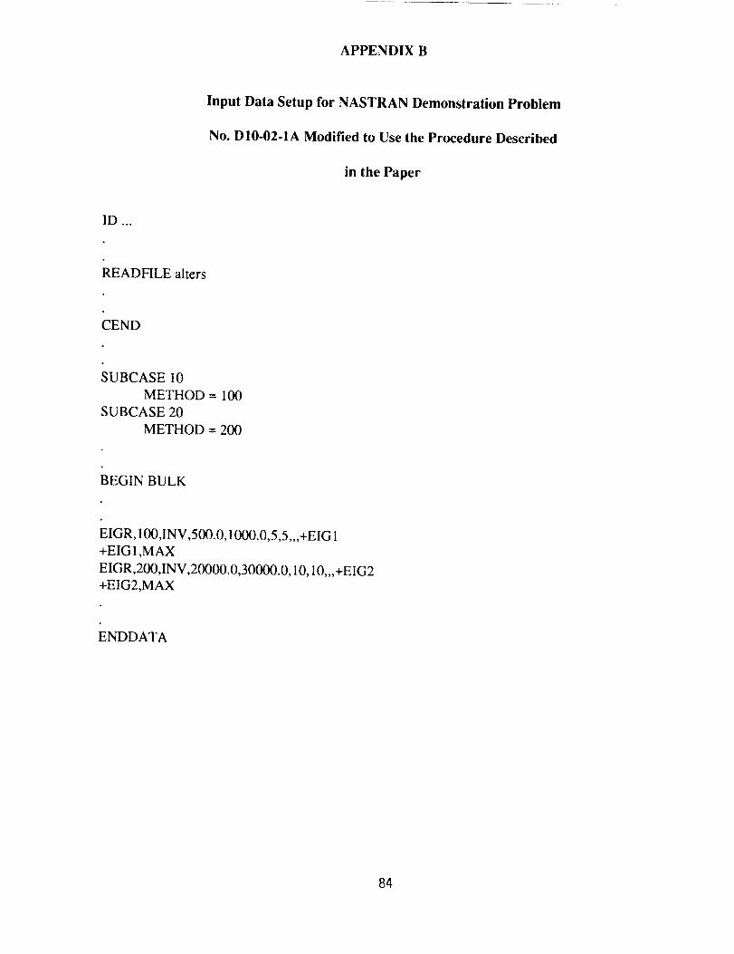
This problem was then modified to use the Inverse Power method and eigensolutions for two
frequency ranges (500.0 - 1000.0 hertz and 20000.0 - 30000.0 hertz) were requested using the
procedure described above. The input data setup is given in Appendix B.
The cyclic frequencies obtained for this case are presented in Table 2. It can be seen that thesefrequencies are subsets of those in Table 1.
Example 2
A variation of NASTRAN Demonstration Problem No. D03-08-1A (without any SUPORT
data) (see Reference 3) was selected for this example. This problem also employs the Givens method
for eigenvalue extraction. The cyclic frequencies obtained for this case are presented in Table 3.
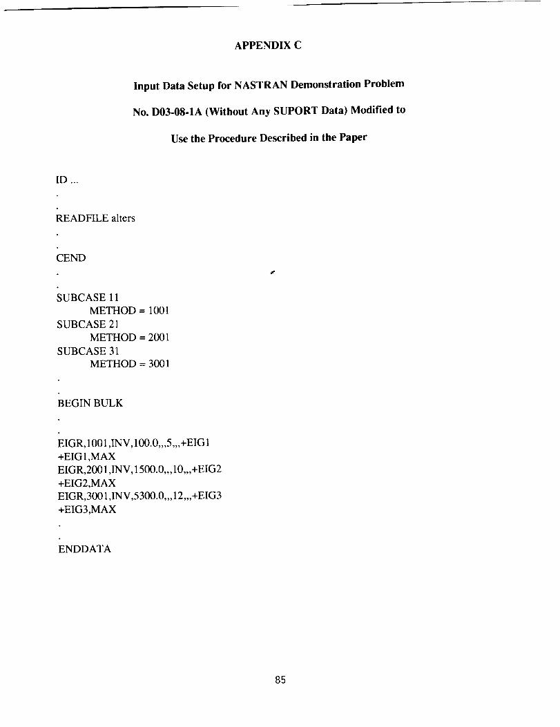
This problem was then modified to use the FEER method and eigensolutions around three shift
points or frequencies (100.0 hertz, 1500.0 hertz and 5300.0 hertz) were requested using the
procedure described above. The input data setup is given in Appendix C.
The cyclic frequencies obtained for this case are presented in Table 4. It can be seen that thesefrequencies are subsets of those in Table 3.
8O
Theresultsof theaboveexamplesclearlydemonstratethevalidity andusefulnessof thepro-posedmethod.
ACKNOWLEDGMENT
TheproceduredescribedabovewasdevelopedaspartofRPK's continuingsupportof itsCRAYversionof NASTRAN at NASA's MarshallSpaceFlight Centerin Huntsville, Alabama. Theauthorsarethankfulto Mr. DavidChristianof NASA-MSFCfor triggeringthestudythatmadethisworkpossible.
CONCLUDING REMARKS
A novel procedure for obtaining eigenvalues and eigenvectors for multiple frequency ranges in
a single NASTRAN execution is presented. The scheme is applicable to normal modes analyses
employing the FEER and Inverse Power methods of eigenvalue extraction. The procedure is
illustrated by examples. The procedure should be particularly helpful in large problems with widely
separated frequency ranges.
REFERENCES
1. The NASTRAN Theoretical Manual, NASA SP-221 (06), January 1981.
2. The NASTRAN User's Manual, NASA SP-222(08), June 1986.
3. The NASTRAN Demonstration Problem Manual, NASA SP-224(05),
December 31, 1978 Edition, Reprinted September 1983.
81
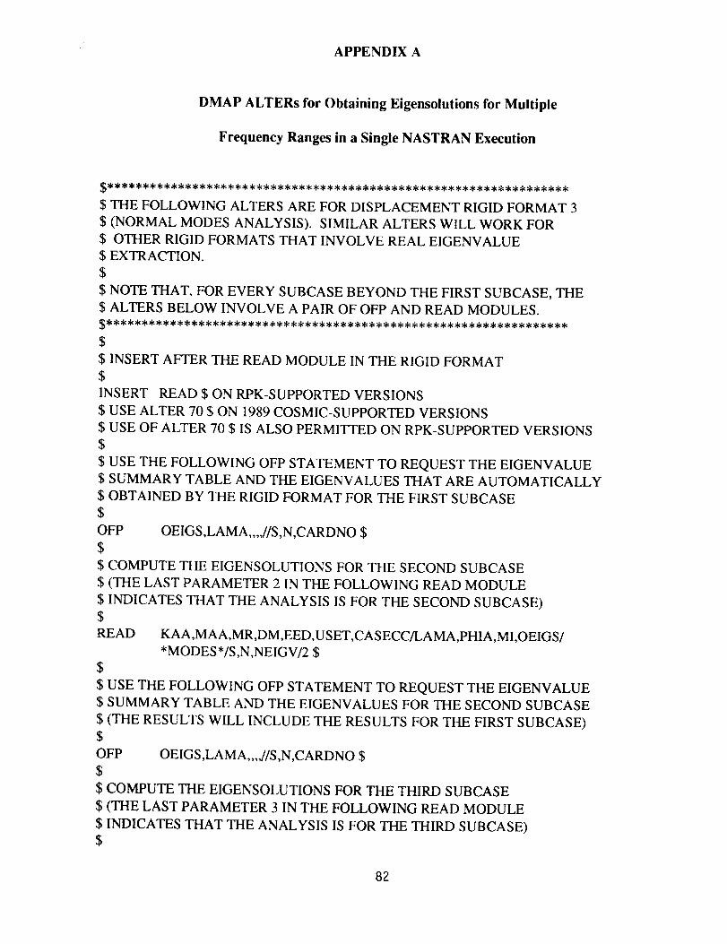
APPENDIX A
DMAP ALTERs for Obtaining Eigensolutions for Multiple
Frequency Ranges in a Single NASTRAN Execution
$ THE FOLLOWING ALTERS ARE FOR DISPLACEMENT RIGID FORMAT 3
$ (NORMAL MODES ANALYSIS). SIMILAR ALTERS WILL WORK FOR
$ OTHER RIGID FORMATS THAT INVOLVE REAL EIGENVALUE$ EXTRACTION.
$
$ NOTE THAT, FOR EVERY SUBCASE BEYOND THE FIRST SUBCASE, THE
$ ALTERS BELOW INVOLVE A PAIR OF OFP AND READ MODULES.
$
$ INSERT AFTER THE READ MODULE IN THE RIGID FORMAT
$INSERT READ $ ON RPK-SUPPORTED VERSIONS
$ USE ALTER 70 $ ON 1989 COSMIC-SUPPORTED VERSIONS
$ USE OF ALTER 70 $ IS ALSO PERMITTED ON RPK-SUPPORTED VERSIONS
$
$ USE THE FOLLOWING OFP STATEMENT TO REQUEST THE EIGENVALUE
$ SUMMARY TABLE AND THE EIGENVALUES THAT ARE AUTOMATICALLY
$ OBTAINED BY THE RIGID FORMAT FOR THE FIRST SUBCASE
$
OFP OEIGS,LAMA .... //S,N,CARDNO $
$
$ COMPUTE THE EIGENSOLUTIONS FOR THE SECOND SUBCASE
$ (THE LAST PARAMETER 2 IN THE FOLLOWING READ MODULE
$ INDICATES THAT THE ANALYSIS IS FOR THE SECOND SUBCASE)$
READ KAA,MAA,MR,DM,EED,USET,CASECC/LAMA,PHIA,MI,OEIGS/
*MODES*/S,N,NEIGV/2 $
$
$ USE THE FOLLOWING OFP STATEMENT TO REQUEST THE EIGENVALUE
$ SUMMARY TABLE AND THE EIGENVALUES FOR THE SECOND SUBCASE
$ (THE RESULTS WILL INCLUDE THE RESULTS FOR THE FIRST SUBCASE)$
OFP OEIGS,LAMA .... //S,N,CARDNO $
$
$ COMPUTE THE EIGENSOLUTIONS FOR THE THIRD SUBCASE
$ (THE LAST PARAMETER 3 IN THE FOLLOWING READ MODULE
$ INDICATES THAT THE ANALYSIS IS FOR THE THIRD SUBCASE)$
82
APPENDIX A
(Continued)
READ KAA,MAA,MR,DM,EED,USET,CASECC/LAMA,PHIA,MI,OEIGS/
*MODES*/S,N,NEIGV/3 $
$
$ USE THE FOLLOWING OFP STATEMENT TO REQUEST THE EIGENVALUE
$ SUMMARY TABLE AND THE EIGENVALUES FOR THE THIRD SUBCASE
$ (THE RESULTS WILL INCLUDE THE RESULTS FOR THE FIRST AND
$ SECOND SUBCASES)
$
OFP OEIGS,LAMA .... //S,N,CARDNO $
$$$$$$$$$READ
COMPUTE THE EIGENSOLUTIONS FOR THE LAST SUBCASE
(THE LAST PARAMETER n IN THE FOLLOWING READ MODULE
SHOULD BE AN INTEGER VALUE CORRESPONDING TO THE LAST
SUBCASE, INDICATING THAT THE ANALYSIS IS FOR THE LAST SUBCASE)
THE FINAL RESULTS (WHICH INCLUDE THE RESULTS FOR ALL OF THE
SUBCASES) ARE AUTOMATICALLY OUTPUT BY THE RIGID FORMAT
$CASE
EQUIV
KAA,MAA,MR,DM,EED,US ET,CASECC/LAMA,PHIA,MI,OEIGS/
*MODES*/S,N,NEIGV/n $
CA SECC,/CASEXX/*TRAN* $
CASEXX,CASECC $
ENDALTER $
83
APPENDIX B
Input Data Setup for NASTRAN Demonstration Problem
No. DI0-02-1A Modified to Use the Procedure Described
in the Paper
ID °°°
READFILE alters
CEND
SUBCASE 10
METHOD = 1130
SUBCASE 20
METHOD = 200
BEGIN BULK
EIGR, 100,INV ,500.0,1000.0,5,5 ,,,+EIG 1
+EIG 1,MAX
EIGR,200,INV,20000.0,30000.0,10,10,,,+EIG2
+EIG2,MAX
ENDDATA
84
APPENDIX C
Input Data Setup for NASTRAN Demonstration Problem
No. D03-08-1A (Without Any SUPORT Data) Modified to
Use the Procedure Described in the Paper
ID °°°
READFILE alters
CEND
SUBCASE 11
METHOD = 1001
SUBCASE 21
METHOD = 2001
SUBCASE 31
METHOD = 3001
BEGIN BULK
EIGR, 1001 ,INV, 100.0,,,5,,,+EIG 1
+EIG1,MAX
EIGR,2001 ,INV, 1500.0,,, 10,,,+EIG2
+EIG2,MAX
EIGR,3001 ,INV,5300.0,,, 12,,,+EIG3
+EIG3,MAX
ENDDATA
85
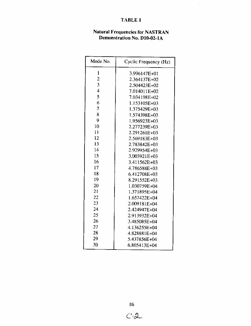
TABLE 1
Natural Frequencies for NASTRAN
Demonstration No. DI0-02-1A
Mode No. Cyclic Frequency (Hz)
1
2
3
4
5
6
7
8
9
10
11
12
13
14
15
16
17
18
19
20
21
22
23
24
25
26
27
28
29
30
3.996147E+01
2.364137E+02
2.504423E+02
7.014011E+02
7.034198E+02
1.153105E+03
1.375429E+03
1.574398E+03
1.956923E+03
2.277239E+03
2.291261E+03
2.569183E+03
2.783842E+03
2.929954E+03
3.003921E+03
3.411562E+03
4.786588E+03
6.412708E+03
8.291552E+03
1.030759E+04
1.371895E+04
1.657422E+04
2.009181E+04
2.424947E+04
2.913932E+04
3.485085E+04
4.136255E+04
4.828881E+04
5.437856E+04
6.805413E+04
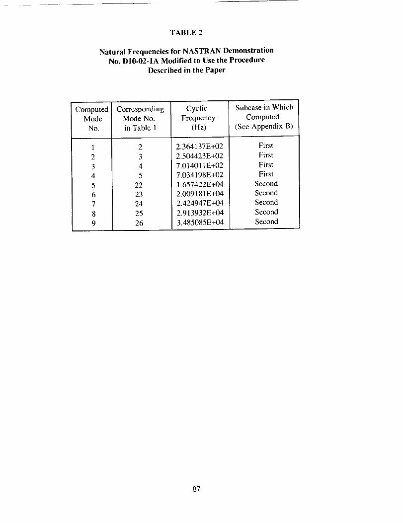
TABLE 2
Natural Frequencies for NASTRAN Demonstration
No. D10-02-1A Modified to Use the Procedure
Described in the Paper
Computed
Mode
No.
1
2
3
4
5
6
7
8
9
CorrespondingMode No.
in Table 1
2
3
4
5
22
23
24
25
26
Cyclic
Frequency
(Hz)
2.364137E+02
2.504423E+02
7.014011E+02
7.034198E+02
1.657422E+04
2.009181E+04
2.424947E+04
2.913932E+04
3.485085E+04
Subcase in Which
Computed
(See Appendix B)
First
First
First
First
Second
Second
Second
Second
Second
87
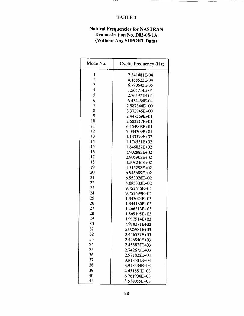
TABLE 3
Natural Frequencies for NASTRAN
Demonstration No. D03-08-1A
(Without Any SUPORT Data)
Mode No. Cyclic Frequency (Hz)
1
23
4
5
6
7
89
1011
12
13
14
15
1617
18
19
20
21
22
23
24
25
26
2728
29
30
31
32
33
34
35
36
37
38
39
40
41
7.341481E-04
4.168523E-04
6.790643E-05
1.505714E-04
2.765971E-04
6.434454E-04
2.987344E+00
3.372945E+00
2.447569E+01
2.682217E+01
6.154903E+017.034309E+01
1.133579E+02
1.174531E+02
1.646037E+02
2.902883E+02
2.905903E+02
4.508246E+02
4.515298E+026.945689E+02
6.953026E+02
8.685333E+02
9.752645E+029.752699E+02
1.343024E+03
1.344180E+03
1.466313E+031.569195E+03
1.912914E+03
1.918371E+03
2.025981E+03
2.446537E+03
2.446840E+03
2.458828E+03
2.742675E+03
2.971822E+03
3.918531E+03
3.918534E+03
4.45185 IE+03
6.261906E+03
8.528055E+03
88
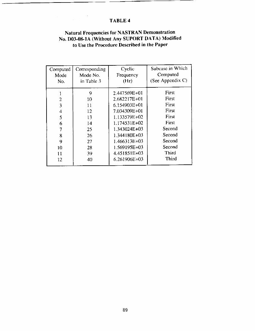
TABLE4
Natural Frequencies for NASTRAN Demonstration
No. D03-08-1A (Without Any SUPORT DATA) Modified
to Use the Procedure Described in the Paper
Computed
Mode
No.
1
2
3
4
5
6
7
8
9
10
11
12
Corresponding
Mode No.
in Table 3
9
10
11
12
13
14
25
26
27
28
39
40
Cyclic
Frequency
(Hz)
2.447569E+01
2.682217E+01
6.154903E+01
7.034309E+01
1.133579E+02
1.174531E+02
1.343024E+03
1.344180E+03
1.466313E+03
1.569195E+03
4.451851E+03
6.261906E+03
Subcase in Which
Computed
(See Appendix C)
First
First
First
First
First
First
Second
Second
Second
Second
Third
Third
89