UNIVERSITA' POLITECNICA DELLE MARCHE

DIPARTIMENTO DI SCIENZE MATEMATICHE

QUADERNO N. 5 - MAGGIO 2006

Lucio Demeio, Stefano Lenci

Forced nonlinear oscillations

of semi-in�nite cables and beams

resting on a unilateral elastic substrate

Dipartimento di Scienze Matematiche

Universit�a Politecnica delle Marche

Via Brecce Bianche 1

I-60131 Ancona, Italy

Forced nonlinear oscillations of semi-in�nite cables and

beams resting on a unilateral elastic substrate

Lucio Demeio

Dipartimento di Scienze Matematiche

Universit�a Politecnica delle Marche

Via Brecce Bianche 1

I-60131 Ancona, Italy

e-mail: demeio@mta01.univpm.it

and

Stefano Lenci

Dipartimento di Architettura, Costruzioni e Strutture

Universit�a Politecnica delle Marche

Via Brecce Bianche 1

I-60131 Ancona, Italy

e-mail: lenci@univpm.it

May 2, 2006

Abstract

In this work, we study the nonlinear oscillations of mechanical systems resting

on a (unilateral) elastic substrate reacting in compression only. We consider both

semi-in�nite cables and semi-in�nite beams, subject to constant distributed load and

to a harmonic displacement applied to the �nite boundary. Due to the nonlinearity

of the substrate, the problem falls in the realm of free-boundary problems, because

the position of the points where the system detaches from the substrate, called Touch

Down Points (TDP), is not known in advance. By an appropriate change of variables,

the problem is transformed into a �xed-boundary problem, which is successively

approached by a perturbative expansion method. In order to detect the mainmechanical

phenomenon, terms up to the second order have to be considered. Two di�erent

regimes have been identi�ed in the behaviour of the system, one below (called subcritical)

1

and one above (called supercritical) a certain critical excitation frequency. In the

latter, energy is lost by radiation at in�nity, while in the former this phenomenon

does not occur and various resonances are observed instead; their number depends on

the statical con�guration around which the system performs nonlinear oscillations.

1 Introduction

This work is aimed at studying the nonlinear forced oscillations of mechanical systems

resting on a (unilateral) elastic substrate reacting in compression only. We consider both

semi-in�nite cables and semi-in�nite beams, subject to a constant distributed load and to

a harmonic displacement applied to the �nite boundary.

Our original motivation was that of describing the laying of marine pipelines [2]. >From

an engineering point of view, the study of the mechanical behaviour of pipelines during the

laying phase is crucial to avoid failures and damages, this phase being the most demanding

in terms of mechanical strength. Some models were proposed by Lenci and Callegari in

[7], and analytical solutions were found in the static case. Here, we study the dynamic

behaviour of pipelines which undergo vertical motions due, e.g., to the oscillations of the

barge on the sea surface.

Because this problem is too diÆcult to be handled with analytical techniques, we focus

on two prototype problems, which, on the one hand, are governed by easier, piece-wise

linear equations, and, on the other hand, are able to describe some of the mechanical

phenomena of the original problem we wish to investigate.

More speci�cally, we focus our attention on the laid part of the pipe and on the �rst

part of the suspended span. These two portions are divided by the so-called Touch-Down

Point (TDP) (Fig. 1). We refer to [4] for the study of the motion of the suspended part

from the TDP to the laying barge. Our simpli�cations are motivated by the fact that

these models capture two main sources of diÆculties, namely, the semi-in�nite length of

the laid beam and the nonlinearity due to the unilateral behaviour of the springs, whose

combined study is the subject of the present work.

The problem considered here falls in the realm of unilateral problems [1], also known

as \moving" or \free" boundary problems [5]; it arises in various engineering applications,

e.g., in the �eld of the dynamics of soil-foundation interactions [16] and in the dynamics

of railways tracks, and it has an interest per se, because it is able to detect in a simple

2

way complex dynamical behaviours. This explains the reason for a joint study of cables

and beams, which is that of investigating how the considered phenomena depend on the

speci�c mechanical model.

Analytical and numerical solutions for the dynamics of a beam on unilateral elastic

springs can be found, e.g., in [15] and [3], respectively. A more mathematically oriented

approach can be found in [13]. The dynamics is governed by a moving-boundary problem

where the position of the TDP is an additional unknown. Since there is no hope to �nd an

exact solution, because of the nonlinearity, we look for an approximate solutions by using

asymptotic analysis [9, 10]. Perturbation techniques were previously applied to study the

nonlinear dynamics of �nite length beams (see, e.g., [11], where the method of multiple

scales is used to attack directly the integro-partial di�erential equation of motion). In this

work the extension to in�nite length is considered.

In our perturbation expansion, the zero order terms correspond to the static solution

obtained in the absence of a time-dependent excitation applied at the boundary, and are

the starting point of the analysis. The �rst order terms are the most important ones, and

permit to understand the resonance behaviour of the system and the questions related

to the wave propagation toward in�nity. In particular, these terms permit to identify

two di�erent regimes, below and above a certain critical excitation frequency, with very

di�erent wave properties [6].

The second order terms give information on the nonlinear coupling between various

modes. Their computation is very hard, and this task will be left for a future work.

However, much information on their behaviour can be inferred from the analysis of their

governing equations; these aspects have been veri�ed numerically elsewhere [8] for the case

of the beam equation.

2 The mathematical models

Here, we introduce the di�erential equations that govern the time-dependent behaviour

of the pro�les of the cables (wave equation) or beams (beam equation). In either case,

the pro�le is represented by the function u(x; t), where 0 � x < +1 is the space variable

and t � 0 the time. A restoring force, with elastic constant k, acts only on the portion

of the spatial domain where the solution u(x; t) is negative. This describes the action of

the elastic substrate that acts in compression only. In our models, we assume that there

3

exists only one point of the domain, x = c, where the pro�le function vanishes, namely

u(c; t) = 0; moreover, the boundary conditions are such that u(x; t) > 0 for 0 � x < c and

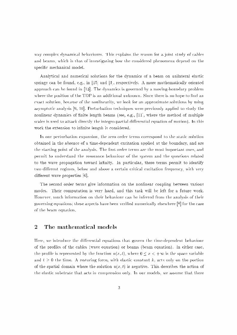
u(x; t) < 0 for c < x <1. The mechanical systems is shown schematically in Fig. 1.

Figure 1: A schematic picture of the considered mechanical systems.

In our analysis, and for both models, the static solution u(x; t) � uS(x) plays an

important role. In this case, c = c0 is a constant, while for the time-dependent solutions

we have that c = c(t) is a function of time. The point x = c is called Touch-Down-Point

(TDP) in the applications, and we adopt this terminology as well. Suitable continuity

conditions on the function u and its spatial derivatives at x = c are also imposed. A

constant load p, representing the compound action of the gravity acceleration and of the

hydrostatic push, is also added to the equations.

In this work, we shall look for time-dependent solutions of the boundary-value problem

that correspond to small oscillations about the static solution. These oscillations are

induced by a time-dependent boundary condition at x = 0, which we will assume of

harmonic behaviour. The TDP x = c(t) will then exhibit oscillating behaviour as well,

and the main quantity of interest in our work is the ratio of the amplitues of the oscillation

of the TDP and the oscillation of the boundary. We shall de�ne these quantities in Section

4.

2.1 Wave equation

If the mechanical system is given by taut inextensible cables, the governing equation is

the wave equation with the addition of suitable terms describing the constant load and

4

the restoring force,

@2u

@t2� v

2@2u

@x2+ p = 0; x < c(t) (1)

@2u

@t2� v

2@2u

@x2+

2u + p = 0; x > c(t); (2)

where v =pT=� is the propagation speed (T is the axial force and � the mass per unit

length), =pk=� (k is the mechanical sti�ness of the unilateral springs) and p = ep=� (ep is

the transversal, uniformly distributed, static load). Note that the same equations govern

the problem of axial vibrations of rods [12] (in which case v =pEA=�, EA being the

axial sti�ness of the rod), and that equation (2) is also known as Klein-Gordon equation.

The boundary condition at x = 0 is u(0; t) = ~U0(1 + " sin t), while at x ! 1we require that u(x; t) be bounded; moreover, we assume that, whenever the equations

support travelling-wave solutions, terms corresponding to waves returning from +1 are

not present, so that only \outgoing" waves (travelling to the right) are admitted. Finally,

the additional continuity conditions at x = c are

u(c�; t) = u(c+; t) = 0 (3)

@u

@x(c�; t) =

@u

@x(c+; t); (4)

where c = c0 for static solutions and c = c(t) for time-dependent solutions. Also, with c�

and c+ we indicate the limits of x! c from the left and from the right, respectively.

It is convenient to write the equations and the boundary conditions in dimensionless

form. It is easily seen that, if we introduce the dimensionless variables t, x and u, given

by t = t, x = x =(vp2) and u = ( 2=p)u, equations (1) and (2) can be cast in the

\universal" form

@2u

@t2� 1

2

@2u

@x2+ 1 = 0; x < c(t) (5)

@2u

@t2� 1

2

@2u

@x2+ u+ 1 = 0; x > c(t); (6)

where we have omitted the hat in order not to burden the notation. The boundary

condition at x = 0 now becomes

u(0; t) = U0(1 + " sin!t); (7)

where U0 = 2 ~U0=p and ! = = . Therefore, we see that the problem depends only upon

two dimensionless parameters, ! and U0, entirely included in the boundary condition at

5

x = 0, while the model equations are free of parameters. The continuity conditions are

still given by equations (3)-(4).

2.2 Beam equation

If the mechanical system is given by beams, the governing equation is the beam equation

with the addition of suitable terms describing gravity and the restoring force; in the original

physical variables, the equations are

@2u

@t2+ b

2@4u

@x4+ p = 0; x < c(t) (8)

@2u

@t2+ b

2@4u

@x4+

2u+ p = 0; x > c(t); (9)

where b2 =pEI=� is a constant (EI is the bending sti�ness of the beam), while and p

have the same meaning as in the wave equation. The boundary conditions are

u(0; t) = ~U0(1 + " sin t) (10)

@2u

@x2(0; t) = 0 (11)

u(x; t) bounded as x!1 (12)

and the additional continuity conditions at x = c are in this case

u(c�; t) = u(c+; t) = 0 (13)

@u

@x(c�; t) =

@u

@x(c+; t); (14)

@2u

@x2(c�; t) =

@2u

@x2(c+; t); (15)

@3u

@x3(c�; t) =

@u3

@x3(c+; t): (16)

Again, we assume that the solution is bounded at in�nity and that there are no travelling

waves returning from +1. In order to cast the equations in dimensionless form, we

again introduce the dimensionless variables t, x and u given by t = t, x = xp =2b and

u = ( 2=p)u. Equations (8) and (9) then become (the hat has again been omitted to

simplify the notation)

@2u

@t2+1

4

@4u

@x4+ 1 = 0; x < c(t) (17)

@2u

@t2+1

4

@4u

@x4+ u+ 1 = 0; x > c(t); (18)

6

which are again free of parameters. The boundary condition at x = 0 takes the form (7)

as for the wave equation, and the problem is seen again to depend upon the same two

parameters ! and U0, with U0 = 2 ~U0=p and ! = = again. The continuity conditions

are still given by equations (13)-(16).

3 The static solutions

The static solutions of the model equations play a very important role in our analysis,

since they give the zero-order terms in our perturbative approach. In this Section, we

derive these solutions for the wave equation and for the beam equation.

3.1 Wave equation

We begin by considering equations (5)-(6), in which we switch o� the time derivatives,

thus obtaining the static equations

�1

2u00S + 1 = 0; x < c0 (19)

�1

2u00S + uS + 1 = 0; x > c0; (20)

where we have indicated with uS(x) the static solution and by c0 the TDP, which is �xed

in this case. The boundary condition at x = 0, in this stationary case, is now uS(0) =

U0, while the continuity conditions imply uS(c�0 ) = uS(c

+0 ) = 0 and u

0S(c

�0 ) = u

0S(c

+0 ).

Equations (19) and (20) with the assigned boundary and continuity conditions are easily

integrated, giving

uS(x) = (x� c0)

�x� U0

c0

�; x < c0 (21)

uS(x) = e(c0�x)

p2 � 1; x > c0 (22)

with the TDP c0 given by

c0 =

p2

2

�p1 + 2U0 � 1

�; (23)

which depends only upon U0.

7

3.2 Beam equation

For the beam equations (17)-(18), by switching o� the time derivatives we obtain:

1

4u(IV )S + 1 = 0; x < c0 (24)

1

4u(IV )S + uS + 1 = 0; x > c0: (25)

The boundary conditions are the same as for the stationary wave equation with the

additional condition u00S(0) = 0, while for the continuity conditions we now add u

00S(c

�0 ) =

u00S(c

+0 ) and u

000S (c

�0 ) = u

000S (c

+0 ). Equations (24) and (25) with the assigned boundary and

continuity conditions are easily integrated, giving

uS(x) = (c0 � x)

"x3 � (2 + c0)(c0 + x)x

6+

U0

c0

#; x < c0 (26)

uS(x) = e(c0�x) [cos(x� c0)� c0 sin(x� c0)]� 1; x > c0 (27)

with c0 given by the solution of the quartic equation

c40 + 4c30 + 6c20 + 6c0 � 6U0 = 0; (28)

which again depends only upon U0. Equation (28) can also be thought of as a linear

equation for U0, with c0 playing the role of a free parameter.

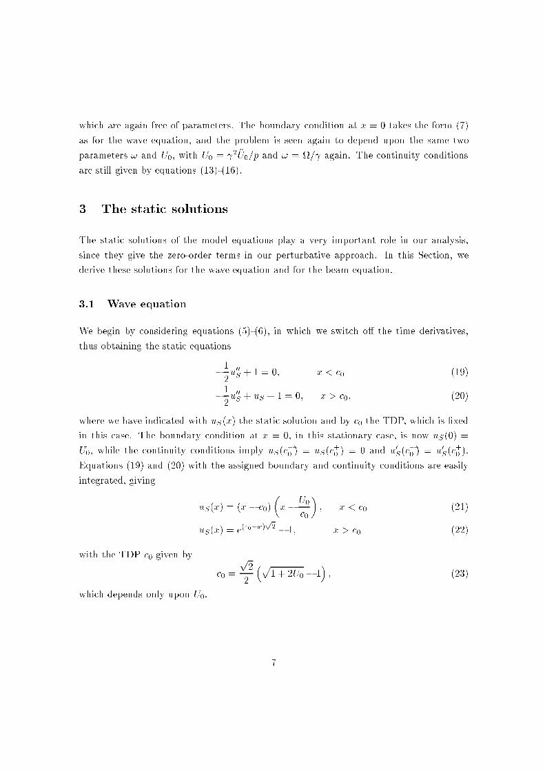
In Figure 2(A) we show the TDP as a function of U0 for the wave equation (solid line)

and for the beam equation (dashed line), for 0 � U0 � 100 and in Figure 2(B) we show

the static solution uS(x), 0 � x � 10, for the wave equation (solid line) and for the beam

equation (dashed line) for U0 = 10. Note that the TDP for the wave equation lies to the

right of the TDP for the beam equation for all the values of U0 considered here.

4 Perturbative approach to the time-dependent model

The moving boundary conditions at x = c(t) for equations (5)-(6) (wave equation), or

equations (17)-(18) (beam equation) make the problem very hard to approach. However,

since we are interested in motions corresponding to small deviations from the static

solution, we approach the problem by perturbative expansions. Before applying the

perturbative expansion, however, we perform a variable transformation which maps the

8

20 40 60 80 100

c0

U0

2.5

5

7.5

10(A) (B)

Figure 2: (A) The Touch-Down-Point c0 for the wave equation (solid line) and for the beam

equation (dashed line) as a function of U0 for 0 � U0 � 100 and (B) the static solution uS(x)

for the wave equation (solid line) and for the beam equation (dashed line) as a function of x,

0 � x � 10, for U0 = 10.

original moving-boundary problem into a �xed-boundary problem, which is then amenable

to asymptotic analysis.

We seek a transformation from the original variables (x; t) to a new set of variables,

(z; �), which maps the line x = c(t) of the (x; t) plane into the line z =constant in the

new (z; �) plane. Of course, there are many transformations that possess this property;

we choose the simplest of all, namely

z =x

c(t)(29)

� = t (30)

u(x; t) = u(zc(t); t) = U(z; t); (31)

in which we keep the original time variable. The same transformation has been used, in a

di�erent context, by Yilmaz [14]. In order not to burden the notation and not to dirty the

pages, we shall not change the notation for the function u, which will now be denoted as

u(z; t), instead of U(z; t). With this transformation, the moving TDP x = c(t) becomes

z = 1 and is now �xed, so that u(1; t) = 0, while x = 0 and x ! 1 correspond to z = 0

and z !1.

After performing the variable transformation to the wave equation and to the beam

equation, we expand the unknown function u(z; t) and the location of the TDP c(t)

(unknown as well) in powers of " according to

u(z; t) = u0(z) + "u1(z; t) + "2u2(z; t) + "

3u3(z; t) +O("4) (32)

9

c(t) = c0 + "c1(t) + "2c2(t) + "

3c3(t) + O("4): (33)

Note that the zero-order terms are independent of time and therefore, with this expansion,

the zero-order quantities will be given by the solutions of the static problems, consistently

with our search for solutions near the static pro�les.

In general, we shall look for solutions that correspond to small periodic oscillations

about the static solutions. Therefore, we shall assume that the functions uk(z; t) and

ck(t), k � 1, admit a Fourier-like expansion of the type

uk(z; t) = gk0(z) +

1Xn=1

[fkn(z) sinn!t + gkn(z) cosn!t] (34)

ck(t) = bk0 +

1Xn=1

[akn sin n!t + bkn cosn!t] : (35)

Our aim is to determine the coeÆcients f , g, a and b of these expansions.

As we mentioned in the Introduction, the main quantity of interest for us is the ratio of

the amplitude of the oscillation of the TDP and the oscillation of the boundary at z = 0.

If we denote by �(") the maximum elongation of the TDP from the static position c0, we

introduce the function

D(U0; !) =�(")

"U0

; (36)

D is called ampli�cation factor, since it gives the measure of the ampli�cation with which

the oscillation at the boundary is re ected on the oscillation of the TDP. In general, the

amplitude � inherits the expansion in powers of " from (33), starting from a �rst-order

term, and therefore the ampli�cation factor also admits a similar expansion, starting from

a term of order zero in ".

4.1 Wave equation

We begin by performing the variable transformation (29)-(31) on the wave equation (5)-

(6). After evaluating all composed derivatives by using the chain rule, we obtain the

transformed di�erential equations for the new unknown function u(z; t):

c2@

2u

@t2+

�_c2z2 � 1

2

�@2u

@z2� 2c _cz

@2u

@t@z+�

2 _c2 � c�c�z@u

@z+ c

2 = 0; z < 1 (37)

10

c2@

2u

@t2+

�_c2z2 � 1

2

�@2u

@z2� 2c _cz

@2u

@t@z+�

2 _c2 � c�c�z +

@u

@z+ c

2(1 + u) = 0; z > 1 (38)

with the boundary conditions

u(0; t) = U0(1 + " sin!t) (39)

u(z; t) bounded as z !1 (40)

and the additional continuity conditions

u(1�; t) = u(1+; t) = 0 (41)

@u

@z(1�; t) =

@u

@z(1+; t): (42)

Next, we introduce the perturbative expansion (32)-(33) into the transformed equations

(37)-(38) and obtain the usual hierarchy of equations by equating to zero the coeÆcients

of the powers of ". The details of the calculations are very long and tedious, and we have

carried them out with the help of a symbolic manipulation program.

To order "0 we have:

1� u000(z)

2 c02= 0; z < 1 (43)

1 + u0(z)�u000(z)

2 c02= 0; z > 1 (44)

to order "1:

@2u1

@t2� 1

2c20

@2u1

@z2� z u0

0(z) �c1(t)

c0+

c1(t) u000(z)

c03

= 0; z < 1 (45)

@2u1

@t2� 1

2c20

@2u1

@z2+ u1(z; t)�

z u00(z) �c1(t)

c0+c1(t) u0

00(z)

c03

= 0; z > 1 (46)

to order "2:

@2u2

@t2� 1

2c20

@2u2

@z2� z u0

0(z) �c2(t)

c0+

c2(t)

c30

u000(z)�

3c1(t)2

2c40u000(z) +

2 z _c1(t)2u00(z)

c02

+z c1(t) u0

0(z) �c1(t)

c02

+z2 _c1(t)

2u000(z)

c02

�

z �c1(t)

c0

@u1

@z� 2 z _c1(t)

c0

@2u1

@z@t+c1(t)

c03

@2u1

@z2= 0; z < 1 (47)

11

@2u2

@t2� 1

2c20

@2u2

@z2+ u2(z; t)�

z u00(z) �c2(t)

c0

+c2(t)

c30

u000(z)�

3c1(t)2

2c40u000(z) +

2 z _c1(t)2u00(z)

c02

+z c1(t) u0

0(z) �c1(t)

c02

+z2 _c1(t)

2u000(z)

c02

�

z �c1(t)

c0

@u1

@z� 2 z _c1(t)

c0

@2u1

@z@t+c1(t)

c03

@2u1

@z2= 0: z > 1 (48)

The boundary conditions associated with this hiererchy of equations are

u0(0) = U0 u0(1) = 0

u1(0; t) = U0 sin !t u1(1; t) = 0 (49)

u2(0; t) = 0 u2(1; t) = 0;

while the continuity conditions on the derivatives (42) have to hold at all orders.

4.1.1 Zero-order solution

Equations (43)-(44), with the boundary conditions for u0 given in (49) are easily integrated

giving

u0(z) = c0

�c0z �

U0

c0

�(z � 1) ; z < 1; (50)

u0(z) = ec0(1�z)

p2 � 1; z > 1: (51)

It is easy to see that these two equations de�ne the same function given in (21)-(22) as the

static solution of the problem, provided that the identi�cation x = c0z between the new

and the old variables is made. The value of c0 is then obtained by using the continuity

condition on the derivative, eq. (42), and is consistent with equation (23).

4.1.2 First-order solution

We obtain the �rst order solution by substituting the expansions (34)-(35) for u1 and c1

in equations (45)-(46), and then equating separately to zero the coeÆcient of cosn!t and

sinn!t for each n. In this way, we obtain an in�nite set of equations from which the

expansion coeÆcients f1n(z); g1n(z); a1n and b1n are determined. Again, the calculations

are rather long and we carried them out with a symbolic manipulation program. The

functions f1n(z) and g1n(z) satisfy non-homogeneous second-order di�erential equations,

12

in which the known term is proportional to some of the coeÆcients a1n and b1n, and are

equipped with the boundary conditions

f11(0) = U0

f1n(0) = 0; n 6= 1

g1n(0) = 0; 8nf1n(1) = g1n(1) = 0 8n:

In addition, the requirements that the functions be bounded as z !1 and that there are

no waves travelling to the left have to be imposed. We show here the di�erential equation

governing f11(z), which gives the only non-vanishing contribution to u1(z; t):

f0011 + 2c20!

2f11 +

hz!

2c0U0 � 2c0 + z!

2(1� z)c0

ia11 = 0; z < 1 (52)

f0011 + 2c20(!

2 � 1)f11 +�z!

2c20

p2� 4c0

�ec0(1�z)=

p2a11 = 0; z > 1: (53)

We notice that the solutions of equation (53) depend crucially upon !: the two linearly

independent solutions of the associated homogeneous equation are of hyperbolic type

(\subcritical" case) if ! < 1 and of oscillatory type (\supercritical" case) if ! > 1. As

shown by the analysis of the higher order terms, the threshold between subcritical and

supercritical behaviour is di�erent at di�erent orders in "; for the second-order terms, for

example, the transition occurs at ! = 1=2. In the subcritical case, the boundary conditions

that the solution be bounded as z ! 1 must be used, while in the supercritical case we

must ensure that there are no travelling waves returning from in�nity.

Subcritical case (! < 1).

Due to the fact that f11 is the only function which satis�es non-homogeneous boundary

conditions for z < 1 and by matching the left and right derivatives at z = 1, we �nd that

f11 and a11 are the only non-vanishing contributions to the solution for u1(z; t) and c1(t);

therefore we obtain

u1(z; t) = f11(z) sin!t (54)

c1(t) = a11 sin!t; (55)

where f11(z) is the solution of equations (52)-(53) with the assigned boundary conditions;

the coeÆcient a11 is then determined by the continuity condition on f011(z) at z = 1. We

have:

a11 =A�(U0; !)

B�(U0; !)(56)

13

where

A�(U0; !) = U0 !5 csc(

p2! c0) c

20

B�(U0; !) =(U0 � c

20)!

4

p2

+ !5c30 cot(

p2! c0)�

! c0

�U0 !

4 cot(p2! c0) + !

3

�1 + c0

q2(1� !2)

��

Supercritical case (! > 1).

Also in this case, only terms with n = 1 are present in the solution, like in the subcritical

case. This time, however, by taking the boundary conditions into account and by matching

the left and right derivatives of f11 and g11 at z = 1, we �nd that the terms proportional

to cos!t are also present, and the solution is given by

u1(z; t) = f11(z) sin!t+ g11(z) cos!t (57)

c1(t) = a11 sin!t + b11 cos!t; (58)

with a11 and b11 given by

a11 =A+(U0; !)

B+(U0; !)(59)

b11 =C(U0; !)

B+(U0; !)(60)

where

A+(U0; !) = U0!c30

"1 + U0! cot(

p2!c0)�

U0 � c20

c0

p2� !c

20 cot(

p2!c0)

#

B+(U0; !) = 2(!2 � 1) c40+

"U0 � c

20p

2��1 + U0! cot(

p2!c0)

�+ !c

30 cot(

p2!c0)

#2C(U0; !) =

p2U0 c

40 !

p!2 � 1 csc(

p2! c0)

To �rst order in ", the maximum elongation �(") of the TDP is given by � = ja11j " in

the subcritical case, and by � =qa211 + b211 " in the supercritical case. In Figure 3, we

show the ampli�cation factor D(U0; !) as a function of ! for three di�erent values of c0:

c0 = 1:02 (solid line, corresponding to U0 = 2:4), c0 = 2 (dashed line, corresponding to

U0 = 6:8) and c0 = 6 (dotted line, corresponding to U0 = 44:5). The results show the

presence of resonances, all lying in the subcritical region, and whose number increases

with increasing U0 or c0.

14

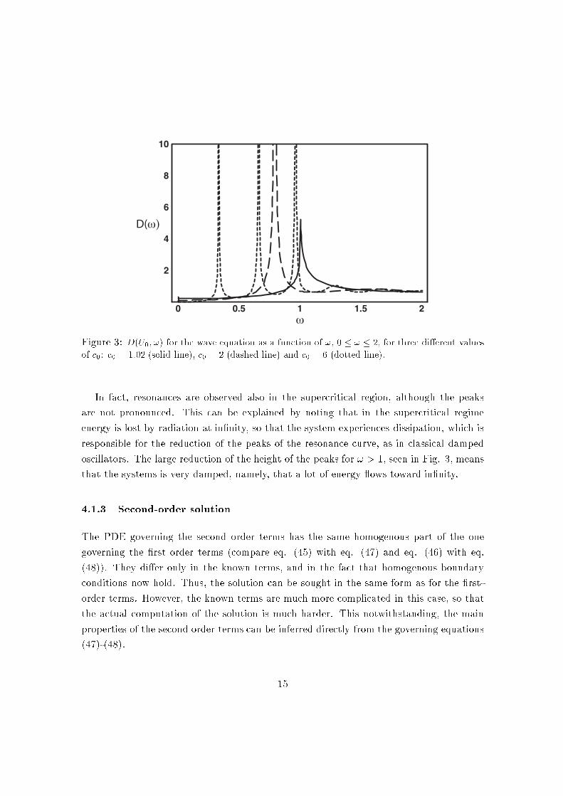
Figure 3: D(U0; !) for the wave equation as a function of !, 0 � ! � 2, for three di�erent values

of c0: c0 = 1:02 (solid line), c0 = 2 (dashed line) and c0 = 6 (dotted line).

In fact, resonances are observed also in the supercritical region, although the peaks

are not pronounced. This can be explained by noting that in the supercritical regime

energy is lost by radiation at in�nity, so that the system experiences dissipation, which is

responsible for the reduction of the peaks of the resonance curve, as in classical damped

oscillators. The large reduction of the height of the peaks for ! > 1, seen in Fig. 3, means

that the systems is very damped, namely, that a lot of energy ows toward in�nity.

4.1.3 Second-order solution

The PDE governing the second order terms has the same homogenous part of the one

governing the �rst order terms (compare eq. (45) with eq. (47) and eq. (46) with eq.

(48)). They di�er only in the known terms, and in the fact that homogenous boundary

conditions now hold. Thus, the solution can be sought in the same form as for the �rst-

order terms. However, the known terms are much more complicated in this case, so that

the actual computation of the solution is much harder. This notwithstanding, the main

properties of the second order terms can be inferred directly from the governing equations

(47)-(48).

15

The most important property is that, since the known term contains expressions proportional

to sin(2!t) and cos(2!t), the second order solutions exhibit superharmonic oscillations

with frequency 2!, and the critical frequency, which is the boundary between the subcritical

and the supercritical regimes, is ! = 1=2. This implies that, for ! < 1=2, the �rst and

second order terms decay exponentially as x!1. In the frequency interval 1=2 < ! < 1,

the �rst order term still decays exponentially, but the second order term behaves like

a propagating wave. Thus, for x large enough, the beam experiences superharmonic

oscillations, although of small (of the order of "2) amplitude, and this is the most evident

consequence of the nonlinearity of the problem. Finally, for ! > 1 both �rst and second

order terms behave like propagating waves, and the harmonic behaviour is dominant.

Of course, the previous argument can be repeated for the terms of order n in ", n > 2,

which exhibit superharmonic behaviour with frequency n!, and which become supercritical

when the frequency overcomes the critical threshold 1=n. However, the amplitudes of this

terms are very small (of the order of "n) and are not interesting from a practical point of

view.

4.2 Beam equation

We now turn to the beam equation (17)-(18). The transformed equations are in this case

c4@

2u

@t2+ c

2 _c2z2@2u

@z2+1

4

@4u

@z4� 2c3 _cz

@2u

@t@z+

c2�2 _c2 � c�c

�z@u

@z+ c

4 = 0; z < 1 (61)

c4@

2u

@t2+ c

2 _c2z2@2u

@z2+1

4

@4u

@z4� 2c3 _cz

@2u

@t@z+

c2�2 _c2 � c�c

�z@u

@z+ c

4(1 + u) = 0; z > 1 (62)

with the boundary conditions

u(0; t) = U0(1 + " sin!t) (63)

@2u

@z2(0; t) = 0 (64)

u(z; t) bounded as z !1 (65)

and the additional continuity conditions

u(1�; t) = u(1+; t) = 0 (66)

16

@u

@z(1�; t) =

@u

@z(1+; t) (67)

@2u

@z2(1�; t) =

@2u

@z2(1+; t) (68)

@3u

@z3(1�; t) =

@3u

@z3(1+; t): (69)

Next, we introduce the perturbative expansion (32)-(33) into the transformed equations

(61)-(62) and obtain the usual hierarchy of equations by equating to zero the coeÆcients

of the powers of ". Again, the details of the calculations are very long and tedious, and

we have carried them out with the help of a symbolic manipulation program.

To order "0 we have:

1 +u(IV )0 (z)

4 c40= 0; z < 1 (70)

1 + u0(z) +u(IV )0 (z)

4 c40= 0; z > 1 (71)

to order "1:

@2u1

@t2+

1

4c40

@4u1

@z4� z u

00(z) �c1(t)

c0� c1(t) u

(IV )0 (z)

c05

= 0; z < 1 (72)

@2u1

@t2+

1

4c40

@4u1

@z4+ u1(z; t)�

z u00(z) �c1(t)

c0� c1(t) u

(IV )0 (z)

c05

= 0; z > 1 (73)

to order "2:

@2u2

@t2+

1

4c40

@4u2

@z4+2 z _c1(t)

2u00(z)

c20

+z c1(t) u

00(z) �c1(t)

c20

� z u00(z) �c2(t)

c0+

z2 _c1(t)

2u000(z)

c02

+

16 c1(t)

2

4 c06

� 24 c02c1(t)

2 + 16 c03c2(t)

16 c08

!u(IV )0 (z)�

z �c1(t)

c0

@u1

@z� 2 z _c1(t)

c0

@2u1

@z@t� c1(t)

c50

@4u1

@z4= 0; z < 1 (74)

@2u2

@t2+

1

4c40

@4u2

@z4+ u2(z; t) +

2 z _c1(t)2u00(z)

c20

+z c1(t) u

00(z) �c1(t)

c20

�

z u00(z) �c2(t)

c0+z2 _c1(t)

2u000(z)

c20

+

16 c1(t)

2

4 c06

� 24 c02c1(t)

2 + 16 c03c2(t)

16 c08

!u(IV )0 (z)�

z �c1(t)

c0

@u1

@z� 2 z _c1(t)

c0

@2u1

@z@t� c1(t)

c50

@4u1

@z4= 0; z > 1: (75)

17

The boundary conditions associated with this hiererchy of equations are

u0(0) = U0; u000(0) = 0; u0(1) = 0

u1(0; t) = U0 sin!t;@2u1

@z2(0) = 0; u1(1; t) = 0 (76)

u2(0; t) = 0;@2u2

@z2(0) = 0; u2(1; t) = 0

while the continuity conditions on the derivatives (67)-(69) have to hold at all orders.

4.2.1 Zero-order solution

Equations (70)-(71), with the boundary conditions for u0 given in (76) are easily integrated

giving

u0(z) = c0 + c02 +

2 c03

3+c0

4

6� z

4c0

4

6+ z

�c0 � c0

2 � c03 � c0

4

3

!+

z3

c0

3

3+c0

4

3

!; z < 1; (77)

u0(z) = �1 + ec0�z c0 (cos(c0 � z c0) + sin(c0 � z c0) c0) ; z > 1: (78)

These two equations de�ne the same function given in (26)-(27) as the static solution of

the problem for the beam equation, with the identi�cation x = c0z. The value of c0 is

then obtained by using the continuity conditions on the derivatives, eq. (67)-(69), and is

consistent with equation (28).

4.2.2 First-order solution

We obtain the �rst order solution by following the same steps outlined in Section 4.1.2 for

the wave equation. The boundary conditions for f1n(z) and g1n(z) now are

f11(0) = U0

f1n(0) = 0; n 6= 1

g1n(0) = 0; 8nf001n(0) = g

001n(0) = 0; 8n

f1n(1) = g1n(1) = 0: 8n

18

and the requirements that the functions be bounded as z ! 1 and that there are no

waves travelling to the left have to be imposed. We show here the di�erential equation

governing f11(z), which gives the only non-vanishing contribution to u1(z; t):

!2

�z + 4!2

c0� z c0 � z c0

2 + z3c0

2 � z c03

3+ z

3c0

3 � 2 z4 c03

3

!a11

� !2f11(z) +

f(IV )11 (z)

4 c04= 0; z < 1 (79)

e(1�z) c0

�sin[(1� z) c0]

h4 + z !

2 (1� c0)i� cos[(1� z) c0]

�z !

2 (1 + c0)�4

c0

��a11 +

(1� !2) f11(z) +

f(IV )11 (z)

4 c04= 0; z > 1: (80)

Again, the solutions of equation (80) depend crucially upon !: two of the four linearly

independent solutions of the associated homogeneous equation exhibit exponential behaviour

(\subcritical" case) if ! < 1 and oscillatory behaviour (\supercritical" case) if ! > 1.

As in the case of the wave equation, the threshold between subcritical and supercritical

behaviour is di�erent at di�erent orders in "; for the second-order terms, for example, the

transition occurs at ! = 1=2. In the subcritical case, the boundary conditions that the

solution be bounded as z ! 1 must be used, while in the supercritical case we must

ensure that there are no travelling waves returning from in�nity.

Subcritical case (! < 1).

As in the case of the wave equation, we �nd that f11 and a11 are the only non-vanishing

contributions to the solution for u1(z; t) and c1(t); therefore we obtain

u1(z; t) = f11(z) sin!t

c1(t) = a11 sin!t;

where f11(z) is the solution of equations (79)-(80) with the assigned boundary conditions;

the coeÆcient a11 is then determined by the continuity conditions on f011(z), f

0011(z) and

f00011(z) at z = 1. In the case of the beam equation, we couldn't �nd a simple expression

for a11 as a function of U0 and !, as we did for the wave equation, and we had to solve

numerically the algebraic system which gives a11 as a solution.

Supercritical case (! > 1).

Also in this case, like for the wave equation, the solution is given by

u1(z; t) = f11(z) sin!t+ g11(z) cos!t

c1(t) = a11 sin!t + b11 cos!t;

19

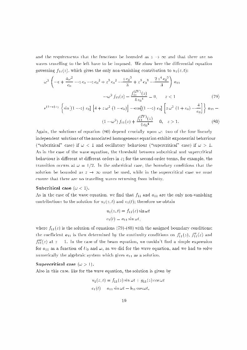
Figure 4: D(U0; !) for the beam equation as a function of !, 0 � ! � 2, for three di�erent values

of c0: c0 = 0:5 (solid line), c0 = 2 (dashed line) and c0 = 6 (dotted line).

with a11 and b11 given by the solution of the algebraic system obtained by matching the

derivatives at z = 1.

The maximum elongation �(") of the TDP is again given by � = ja11j " in the subcritical

case, and by � =qa211 + b

211 " in the supercritical case. In Figure 4, we show the

ampli�cation factor D(U0; !) as a function of ! for three di�erent values of c0: c0 = 0:5

(solid line, corresponding to U0 = 0:8), c0 = 2 (dashed line, corresponding to U0 = 14)

and c0 = 6 (dotted line, corresponding to U0 = 402). The results are similar to the ones of

the wave equation, with the presence of marked resonances in the subcritical region, and

whose number increases at increasing U0 or c0.

Also in this case, there exist very weak resonances in the supercritical regime, represented

by small amplitude peaks; however, due to the choice of the parameters, they are not visible

in Figure 4.

4.2.3 Second-order solution

The computation of the second order terms is here even harder than in the case of Section

4.1.3, but the main properties of the solution can still be understood by examining the

governing equation. Nicely enough, for ! < 1=2 the �rst and second order terms still

20

decay exponentially as x ! 1; for 1=2 < ! < 1 and for x large enough, the beam

experiences superharmonic oscillations, although of small amplitude; and for ! > 1 both

�rst and second order terms behave like propagating waves, and the harmonic behaviour

is dominant.

We conclude that the wave and the beam equations share the samemechanical behaviour

with respect to the problem considered here.

5 Conclusions and outlook

The nonlinear dynamics of semi-in�nite beams and cables resting on a unilateral elastic

substrate has been investigated by means of a classical perturbative approach, after an

appropriate change of variables which transforms the moving boundary problem into one

with �xed boundaries.

Two di�erent regimes have been identi�ed, one below (called subcritical) and one above

(called supercritical) a certain critical excitation frequency. In the latter, energy is lost by

radiation at in�nity, while in the former this phenomenon does not occur. On the contrary,

in the subcritical regime various resonances are observed; their number depends on the

statical con�guration around which the system performs nonlinear oscillations and they

are absent, or better, less pronounced in the supercritical regime, due to the dissipation

by radiation.

The coupling between the nonlinearity and the unboundedness of the domain is studied,

and it is shown that, in the subcritical regime, far enough from the TDP in the direction

of the unbounded boundary, the dominant oscillation is superharmonic, although its

amplitude is orders of magnitude smaller than the amplitude of the harmonic excitation.

Finally, it has been shown that beams and cables share the previous mechanical properties,

which therefore are supposed to be very general, in spite of the known di�erent behaviour

of these two mechanical systems in terms of wave propagation.

Various developments are possible and worthy. The �rst one is certainly the computation

of the second order terms, which are expected to con�rm the predictions of Sections 4.1.3

and 4.2.3 and to show the presence of other resonances. Then, it would be interesting to

use more sophisticated analytical tools, such as the multiple scales method, to get a more

re�ned solution. In this respect, we note that the problem would be particularly enticing,

21

because both slow time scales and slow spatial scales would be required.

By the multiple scales method one can also approach the problem of nonlinear normal

modes, which will allow a deep investigation of the nonlinearity of the model.

Of course, the �nal objective is that of considering the full J-lay problem which actually

motivates this work. However, the passage to (very) large displacement is not expected

to be easily solved.

References

[1] Del Piero, G., Maceri, F. (eds), 1985,Unilateral problems in structural analysis, CISM

Courses and Lectures n. 288.

[2] Callegari, M., Carini, C.B., Lenci, S., Torselletti, E., Vitali, L., 2003, \Dynamic

Models of Marine Pipelines for Installation in Deep and Ultra-deep Waters: Analytical

and Numerical Approaches," Proc. of AIMETA03, Ferrara, 9-12 Sept. 2003 (CD-rom).

[3] Celep, Z., Malaika, A., Abu-Hussein, M., 1989, \Forced vibrations of a beam on a

tensionless foundation," J. Sound Vibration, 128(2), 235-246.

[4] Couliard, P.-Y., Langley, R.S., 2001, \Nonlinear dynamics of deep-water moorings,"

Proc. of OMAE'01, Rio de Janeiro, Brasil.

[5] Crank, J., 1984, Free and Moving Boundary Problems, Oxford University Press.

[6] Doyle, J.F., 1989, Wave propagation in structures, Springer-Verlag.

[7] Lenci, S., Callegari, M., 2005, \Simple analytical models for the J-lay problem," Acta

Mechanica, 178(1-2), 23-39.

[8] Lenci, S., Lancioni, G., 2006, \An analytical and numerical study of the nonlinear

dynamics of a semi-in�nite beam on unilateral Winkler soil," Proc. of World Congress

on Computational Mechanics (WCCM7), Las Vegas, CA, U.S.A., July 16-22, 2006

(CD-rom).

[9] Nayfeh, A., Perturbation Methods, Wiley-Interscience, NY, 1973.

[10] Nayfeh, A., Balachandran, B., Applied Nonlinear Dynamics, Wiley-Interscience, NY,

1995.

22

[11] Chin, C.-M., Nayfeh, A., 1999, \Three-to-One Internal Resonances in Parametrically

Excited Hinged-Clamped Beams," Nonlin. Dyn., 20, 131-158.

[12] Kolsky H., 1963, Stress Waves in Solids, Dover Publications.

[13] Toscano, R., \Un problema dinamico per la piastra su suolo elastico unilaterale,"

in Unilateral problems in structural analysis, Del Piero, G., Maceri, F. (eds), 1985,

CISM Courses and Lectures n. 288, p. 375-387 (in italian).

[14] Yilmaz E., 2003, \One dimensionale Schrodinger equation with two moving

boundaries," ArXiv:math-ph/030206 v2 5 Feb 2003.

[15] Weitsman, Y., 1970, \On foundation that reacts in compression only," ASME J. Appl.

Mech., 37(4), 1019-1030.

[16] Wolf, J.P., 1988, Soil-Structure-Interaction Analysis in Time Domain, Prentice Hall,

Englewood Cli�s, New Jersey.

23