Embed Size (px)
Citation preview

FAULT TOLERANT OPERATIONS OF INDUCTION MOTOR-DRIVE SYSTEMS
by
Chia-Chou Yeh, B.S., M.S.
A Dissertation submitted to the Faculty of the Graduate School, Marquette University,
in Partial Fulfillment of the Requirements for
the Degree of
DOCTOR OF PHILOSOPHY
Milwaukee, Wisconsin May, 2008

ii
Preface
FAULT TOLERANT OPERATIONS OF INDUCTION MOTOR-DRIVE SYSTEMS
Chia-Chou Yeh
Under the Supervision of Professor Nabeel A. O. Demerdash at
Marquette University
This dissertation presents fault-tolerant / “limp-home” strategies of ac motor soft starters and
adjustable-speed drives (ASDs) when experiencing a power switch open-circuit or short-circuit
fault. The present low-cost fault mitigation solutions can be retrofitted into the existing off-the-
shelf soft starters and ASDs to enhance their reliability and fault tolerant capability, with only
minimum hardware modifications. The conceived fault-tolerant soft starters are capable of
operating in a two-phase mode in the event of a thyristor/SCR open-circuit or short-circuit
switch-fault in any one of the phases using a novel resilient closed-loop control scheme. The
performance resulting from using the conceived soft starter fault-tolerant control has
demonstrated reduced starting motor torque pulsations and reduced inrush current magnitudes.
Small-signal model representation of the motor-soft starter controller system is also developed
here in order to design the closed-loop regulators of the control system at a desired bandwidth to
render a good dynamic and fast transient response. In addition, the transient motor performance
under these types of faults is investigated using analytical closed-form solutions, the results of
which are in good agreement with both the detailed simulation and experimental test results of the
actual hardware.
As for ASDs, a low-cost fault mitigation strategy, based on a quasi-cycloconverter-based
topology and control, for low-speed applications such as “self-healing/limp-home” needs for
vehicles and propulsion systems is developed. The present approach offers the potential of
mitigating both transistor open-circuit and short-circuit switch faults, as well as other drive-
related faults such as faults occurring in the rectifier bridge or dc-link capacitor. Furthermore,

iii
some of the drawbacks associated with previously known fault mitigation techniques such as the
need for accessibility to a motor neutral, the need for larger size dc-link capacitors, or higher dc-
bus voltage, are overcome here using the present approach. Due to its unique control algorithm,
torque pulsations are introduced as a result of the non-sinusoidal current waveforms. Meanwhile,
application considerations and opportunities for practical use of the conceived design are also
investigated here in this work. The results of this research suggest that the conceived approach is
best suited for partial motor-loading operating condition, which is normally the case for many
practical industrial applications where the motors are usually oversized. The reason for choosing
to operate under such conditions is the resulting reduced torque pulsations that the motor will
experience when supplied by the conceived topology at light-load conditions. In addition, the
negative impact of inverter switch fault on motor performance is also analyzed in this work using
the averaged switching function modeling concept. Simulation and experimental work have been
performed to demonstrate the efficacy and validity of the conceived fault-tolerant solutions for
induction motor fault mitigation applications.

iv
Acknowledgement
First of all, I wish to express my sincere and deepest gratitude to my advisor, Professor
Nabeel A. O. Demerdash, for his encouragement, time, and expert technical guidance throughout
the completion of this work. Without his open-mindedness and patient guidance, this dissertation
would not come to exist. His endless hours of advice and help in my research work are very much
appreciated and will always be remembered. Our discussions involve not only technical matters,
but also life in general. In fact, he serves as a father figure to me. It is my extreme privilege to
have him as my advisor as well as my dear friend. His famous quote: “No question is a stupid
question” will always be buried in my mind.
I would also like to extend my deepest gratitude to my other dissertation committee
members, namely Prof. Ronald H. Brown and Prof. Edwin E. Yaz of Marquette Univesity, Dr.
Thomas W. Nehl of Delphi Automotive Research, and Dr. Russel J. Kerkman of Allen Bradley-
Rockwell Automation, for their precious time, support, and useful suggestions/insights.
I am also very grateful to my internship employer, Eaton Corporation, when I was with them
for the majority part of my Ph.D. studies, for the technical experience, skills and knowledge that I
gained which enabled the completion of this work. Furthermore, I wish to thank my co-workers,
Madhav D. Manjrekar, Ian T. Wallace, Vijay Bhavaraju, Jun Kikuchi, and Edward F. Buck for all
the helpful discussions in various projects.
In addition, I wish to acknowledge the financial support from the US National Science
Foundation under Grant ECS-0322974 and the Rev. John P. Raynor Fellowship. I also wish to
thank the Marquette University EECE department, professors, and support staff, especially Jean
M. Weiss, for providing the environment that made this research work possible.

v
The support of the Eaton Corporation, Allen Bradley-Rockwell Automation, and A. O.
Smith Corporation, in providing the test motors, drives, and other electronic equipment, is
gratefully acknowledged. The experimental portion of this research work would not be possible
without their support and generosity.
I also wish to extend special thanks to my dearest friends, Ahmed Sayed-Ahmed, Behrooz
Mirafzal, Gennadi Y. Sizov, and Anushree Kadaba for their support, useful insights, and fruitful
discussions throughout my graduate studies at Marquette University. The time when we all spent
together in the lab is something I will never forget. I will definitely miss the moment and fun in
our weekly “Tuesday Pizza”.
Most importantly, I would like to thank a special person, my lovely wife Huili, for her
infinite patience, kindness, and endless love throughout this period. Her continued support and
belief in me in things I wish to accomplish in my life will always be remembered. Her strong
character has kept me motivated in the completion of this work. She definitely plays a major role
in my life. Finally, I owe my deepest appreciation and special thanks to my family for their love,
support, and encouragement throughout my life and education. This dissertation would not be
possible without them.
There are many other people who have helped me in some ways in my research work.
Although I cannot mention each one of their names, I never forget their kindness. Once again, I
would like to express my greatest gratitude to all these people. Thank you all, it is good knowing
you.
Chia-Chou Yeh
May 2008

vi
Contents
List of Figures ......................................................................................................... x
List of Tables.......................................................................................................xvii
1 Introduction ..................................................................................................... 1 1.1 Motivation behind This Work ...................................................................................... 1 1.2 Literature Search Surveying Preceding Work.............................................................. 6 1.3 Objectives and Contributions ..................................................................................... 16 1.4 Dissertation Organizations ......................................................................................... 18 1.5 Summary .................................................................................................................... 19
2 Transient Analysis of Induction Motor-Soft Starter ................................. 20 2.1 Introduction ................................................................................................................ 20 2.2 Soft Starters ................................................................................................................ 21
2.2.1 Topology ....................................................................................................... 21 2.2.2 Principles of Operations ................................................................................ 22
2.3 Closed-Form Derivation............................................................................................. 25 2.3.1 Closed-Form Expressions of Motor Phase Voltages..................................... 25 2.3.2 Closed-Form Expressions of Motor Phase Currents ..................................... 34
2.4 Analysis of Failure Modes and Effects ...................................................................... 38 2.4.1 Short-Circuit SCR Fault ................................................................................ 39 2.4.2 Open-Circuit SCR Fault ................................................................................ 44
2.5 Summary .................................................................................................................... 46
3 Fault Tolerant Soft Starter........................................................................... 48 3.1 Introduction ................................................................................................................ 48 3.2 Principles of Fault Tolerant Operations ..................................................................... 49
3.2.1 Modified Topology ....................................................................................... 50 3.2.2 A Resilient Closed-Loop Two-Phase Control Scheme ................................. 52
3.3 Small-Signal Modeling of Motor-Soft Starter Controller .......................................... 56 3.3.1 Transfer Function of Controller .................................................................... 59 3.3.2 Transfer Function of Induction Motor........................................................... 59

vii
3.3.3 Nonlinear Representation of Soft Starter ...................................................... 62 3.3.4 Small-Signal Model Representation of Overall System................................ 65
3.4 Design Procedures of Soft Starter PI Controllers....................................................... 66 3.4.1 Voltage Control Loop.................................................................................... 66 3.4.2 Current Control Loop .................................................................................... 68
3.5 Summary .................................................................................................................... 71
4 Circuit Simulations of Fault Tolerant Soft Starter.................................... 74 4.1 Introduction ................................................................................................................ 74 4.2 Circuit Simulation Model........................................................................................... 75 4.3 Verifications between Closed-Form Analytical and Simulation Results ................... 79
4.3.1 Healthy Condition ......................................................................................... 79 4.3.2 Short-Circuit SCR Switch Fault Condition ................................................... 84
4.4 Motor Performance under Fault Tolerant Operations ................................................ 85 4.5 Summary .................................................................................................................... 90
5 Hardware Experiments of Fault Tolerant Soft Starter............................. 95 5.1 Introduction ................................................................................................................ 95 5.2 Hardware Prototype.................................................................................................... 96 5.3 Experimental Results................................................................................................ 101
5.3.1 Comparisons with Simulation and Analytical Results ................................ 101 5.3.2 Motor Performance under Fault Tolerant Operations ................................. 110
5.4 Summary .................................................................................................................. 113
6 Analysis of Failure Mode and Effect of Inverter Switch Faults on Motor Performance................................................................................................. 121 6.1 Introduction .............................................................................................................. 121 6.2 Averaged Switching Function Model....................................................................... 122
6.2.1 Motor Phase Voltage Representations ........................................................ 124 6.2.2 Averaged Switching Function Formulations............................................... 125
6.3 Analysis of Failure Modes and Effects .................................................................... 130 6.3.1 Short-Circuit Switch Fault .......................................................................... 131
6.3.1.1 Circuit Simulation Model............................................................ 133 6.3.1.2 Analytical and Simulation Results .............................................. 136
6.3.2 Open-Circuit Switch Fault .......................................................................... 144 6.3.2.1 Simulation Results ...................................................................... 148

viii
6.4 Summary .................................................................................................................. 160
7 A Quasi-Cycloconverter-Based Topology and Control for Inverter Fault Mitigation..................................................................................................... 162 7.1 Introduction .............................................................................................................. 162 7.2 Present Fault Mitigation Topology and Control....................................................... 167
7.2.1 Operating Principle of Present Topology.................................................... 167 7.2.2 Discrete-Frequency Control Algorithm....................................................... 172
7.3 Summary .................................................................................................................. 179
8 Simulation and Experimental Results of Inverter-Motor Fault Tolerant Operation ..................................................................................................... 181 8.1 Introduction .............................................................................................................. 181 8.2 Simulation Performance ........................................................................................... 182
8.2.1 Circuit Simulation Model............................................................................ 182 8.2.2 Simulation Results....................................................................................... 186
8.2.2.1 The No-Load Case ...................................................................... 186 8.2.2.2 Limp-Home Operation of the Conceived Topology under Inverter
Fault Case.................................................................................... 187 8.2.2.3 Starting Performance of the Conceived Topology...................... 198
8.3 Experimental Validations ......................................................................................... 204 8.3.1 The No-Load Case ...................................................................................... 207 8.3.2 Limp-Home Operation of the Conceived Topology under Inverter Fault Case ……………………………………………………………………………..207 8.3.3 Starting Performance of the Conceived Topology ...................................... 222
8.4 Application Considerations and Opportunities ........................................................ 224 8.5 Summary .................................................................................................................. 229
9 Conclusions, Contributions, and Suggested Future Work...................... 230 9.1 Summary and Conclusions....................................................................................... 230 9.2 Contributions of this Work....................................................................................... 237 9.3 Future Investigations ................................................................................................ 238
Bibliography........................................................................................................ 240
Appendix A Designs and Specifications of Hardware Prototype ............ 250 A.1 Introduction .............................................................................................................. 250 A.2 System Descriptions ................................................................................................. 250

ix
A.2.1 Motor Design Specifications and Datasheets .............................................. 255 A.2.2 Soft Starter and Quasi-Cycloconverter Designs.......................................... 259 A.2.3 PWM Drive ................................................................................................. 262 A.2.4 DSP Controller Board ................................................................................. 262 A.2.5 Signal Conditioning Circuits ....................................................................... 265 A.2.6 Data Acquisition System............................................................................. 268

x
List of Figures
Figure 1.1: Types of inverter switch failure modes under investigation......................................... 5 Figure 1.2: Categorization of various “limp-home” strategies for three-phase ac motor-drives. ... 7 Figure 1.3: Fault-tolerant inverter topology by Liu et al. [49] and Elch-Heb et al. [50]. ............... 8 Figure 1.4: Fault-tolerant inverter topology by Van Der Broeck et al. [52] and Ribeiro et al. [44].
.................................................................................................................................... 11 Figure 1.5: First fault-tolerant inverter topology by Bolognani et al. [40]. .................................. 13 Figure 1.6: Second fault-tolerant inverter topology by Bolognani et al. [40]. .............................. 14 Figure 2.1: Conventional three-phase soft starter topology. ......................................................... 23 Figure 2.2: Definitions of firing angles......................................................................................... 23 Figure 2.3: Voltage ramp profiles. ................................................................................................ 25 Figure 2.4: (a) 3-phase conduction mode. (b) 2-phase conduction mode. ................................... 26 Figure 2.5: Healthy transient current space-vector plot during soft starting................................. 30 Figure 2.6: Healthy transient three-phase currents during soft starting. ....................................... 30 Figure 2.7: T-equivalent circuit model (h is the harmonic order)................................................. 33 Figure 2.8: Analytical solution of healthy three-phase line-to-neutral motor voltage waveforms at
operating conditions of 60φ = and 90α = . .......................................................... 33
Figure 2.9: Analytical solution of healthy three-phase current waveforms at transient conditions of 60φ = , 90α = , and motor speed of 200-r/min................................................. 37
Figure 2.10: Failure modes in soft starter circuit. (a) Short-circuit fault. (b) Open-circuit fault.39 Figure 2.11: Transient current space-vector plot during soft starting under a short-circuit SCR
fault. ......................................................................................................................... 40 Figure 2.12: Three-phase line-to-neutral motor voltage waveforms from analytical solution under
a short-circuit SCR fault........................................................................................... 42 Figure 2.13: Analytical solution of three-phase current waveforms at transient conditions of
60φ = , 90α = , and motor speed of 400-r/min under a short-circuit SCR fault. 43
Figure 3.1: Industrial type three-phase soft starter topology. ....................................................... 51 Figure 3.2: Modified version of soft starter with fault tolerance/isolation capabilities. ............... 51 Figure 3.3: Post-fault soft starter configuration. ........................................................................... 52 Figure 3.4: Present closed-loop two-phase control for fault tolerant soft starter. ......................... 54 Figure 3.5: Reference voltage ramp profile. ................................................................................. 54 Figure 3.6: Simplified control system representation of motor-soft starter controller.................. 58

xi
Figure 3.7: Voltage control loop. .................................................................................................. 58 Figure 3.8: Current control loop. .................................................................................................. 58 Figure 3.9: Transfer function of per-phase induction motor model.............................................. 62 Figure 3.10: A plot of motor phase voltage (rms) versus αV using Equation (3.14). ................... 65 Figure 3.11: Bode plot of voltage control feedback loop system. (a) Open-loop transfer function.
(b) Closed-loop transfer function.............................................................................. 69 Figure 3.12: Bode plot of current control feedback loop system. (a) Open-loop transfer function.
(b) Closed-loop transfer function.............................................................................. 72 Figure 4.1: Schematic of motor-soft starter power structure in Matlab-Simulink [91]. ............... 76 Figure 4.2: Block diagram of soft starter controller in Matlab-Simulink [91].............................. 78 Figure 4.3: Healthy three-phase line-to-neutral motor voltage waveforms at operating conditions
of 60φ = and 90α = . (a) Analytical. (b) Simulation. ........................................ 81
Figure 4.4: Healthy three-phase current waveforms at transient conditions of 60φ = , 90α = , and motor speed of 200-r/min. (a) Analytical. (b) Simulation. ................................ 82
Figure 4.5: RMS values of healthy three-phase stator currents from analytical solution and dynamic simulation. ................................................................................................... 84
Figure 4.6: Three-phase line-to-neutral motor voltage waveforms at operating conditions of 60φ = and 90α = under a short-circuit SCR fault. (a) Analytical.
(b) Simulation............................................................................................................. 86
Figure 4.7: Three-phase current waveforms at transient conditions of 60φ = , 90α = , and motor speed of 400-r/min under a short-circuit SCR fault. (a) Analytical. (b) Simulation............................................................................................................. 87
Figure 4.8: RMS values of three-phase stator currents from analytical solution and dynamic simulation under a short-circuit SCR fault. ................................................................ 89
Figure 4.9: Simulation results of three-phase current waveforms. (a) 3-phase open-loop control. (b) 2-phase open-loop control. (c) Proposed 2-phase closed-loop control................ 92
Figure 4.10: Simulation results of current space-vector plots. (a) 3-phase open-loop control. (b) 2-phase open-loop control. (c) Proposed 2-phase closed-loop control. ............. 93
Figure 4.11: Simulation results of motor developed torque. (a) 3-phase open-loop control. (b) 2-phase open-loop control. (c) Proposed 2-phase closed-loop control. ............. 94
Figure 5.1: Schematic of experimental setup of induction motor-soft starter system................... 98 Figure 5.2: Test rigs. (a) Soft starter. (b) Induction motor and dynamometer. ........................... 99 Figure 5.3: Healthy three-phase line-to-neutral motor voltage waveforms. (a) Test.
(b) Simulation. (c) Analytical.................................................................................. 104 Figure 5.4: Healthy three-phase current waveforms. (a) Test. (b) Simulation. (c) Analytical. 105 Figure 5.5: Three-phase line-to-neutral motor voltage waveforms under a short-circuit SCR fault.
(a) Test. (b) Simulation. (c) Analytical. ................................................................. 107 Figure 5.6: Three-phase current waveforms under a short-circuit SCR fault. (a) Test.
(b) Simulation. (c) Analytical.................................................................................. 108
xii
Figure 5.7: Test results obtained under direct-line-starting. (a) Three-phase motor currents. (b) Motor developed torque...................................................................................... 114
Figure 5.8: Three-phase motor currents obtained under 3-Phase Open-Loop Control. (a) Test. (b) Simulation. .......................................................................................... 115
Figure 5.9: Motor developed torque obtained under 3-Phase Open-Loop Control. (a) Test. (b) Simulation. .......................................................................................... 116
Figure 5.10: Three-phase motor currents obtained under 2-Phase Open-Loop Control. (a) Test. (b) Simulation. ........................................................................................ 117
Figure 5.11: Motor developed torque obtained under 2-Phase Open-Loop Control. (a) Test. (b) Simulation. ........................................................................................ 118
Figure 5.12: Three-phase motor currents obtained under 2-Phase Closed-Loop Control. (a) Test. (b) Simulation. ........................................................................................ 119
Figure 5.13: Motor developed torque obtained under 2-Phase Closed-Loop Control. (a) Test. (b) Simulation. ........................................................................................ 120
Figure 6.1: Types of inverter switch failure modes under investigation..................................... 123 Figure 6.2: Inverter circuit. ......................................................................................................... 123 Figure 6.3: PWM switching function, H1, of switch, S1, of inverter leg-a.................................. 127 Figure 6.4: Switching function expressed over a switching period of switch, S1. ...................... 127 Figure 6.5: Schematic of induction motor-drive power structure in Matlab-Simulink [91]. ...... 134 Figure 6.6: Three-phase motor phase voltages during short-circuit switch fault condition.
(a) Analytical. (b) Simulation.................................................................................. 138 Figure 6.7: FFT spectra of simulated three-phase motor phase voltages during short-circuit
switch fault condition. (a) Phase-a. (b) Phase-b. (c) Phase-c. ............................... 139 Figure 6.8: Simulation results of three-phase motor currents during pre- and post-fault short-
circuit switch fault conditions (fault occurs at t = 1.3 sec). ..................................... 140 Figure 6.9: FFT spectra of simulated three-phase motor currents during short-circuit switch fault
condition. (a) Phase-a. (b) Phase-b. (c) Phase-c.................................................... 141 Figure 6.10: Simulation results of motor speed during short-circuit switch fault condition (fault
occurs at t = 1.3 sec). (a) Time-domain profile during pre- and post-fault. (b) FFT spectrum during post-fault. ....................................................................... 142
Figure 6.11: Simulation results of motor developed torque during short-circuit switch fault condition (fault occurs at t = 1.3 sec). (a) Time-domain profile during pre- and post-fault. (b) FFT spectrum during post-fault....................................................... 143
Figure 6.12: Inverter circuit topology with an open-circuit fault at switch S1. ........................... 145 Figure 6.13: Simulation waveforms of motor quantities during pre- and post-fault conditions
(open-circuit switch fault occurred at switch S1 at t = 1.3 sec). ............................. 147 Figure 6.14: Simulation results of three-phase motor currents during pre- and post-fault open-
circuit switch fault conditions. (a) Healthy. (b) Post-Fault. ................................. 154 Figure 6.15: FFT spectra of simulated three-phase motor currents during open-circuit switch fault
condition. (a) Healthy case in all phases. (b) Faulty case of ia. (c) Faulty case of ib. (d) Faulty case of ic................................................................................................. 155

xiii
Figure 6.16: Simulation results of dc link voltage during open-circuit switch fault condition (fault occurs at t = 1.3 sec). (a) Time-domain profile during pre- and post-fault. (b) FFT spectrum during post-fault. (c) Close-up view of FFT spectrum of Figure (b)..... 156
Figure 6.17: Simulation results of motor developed torque during open-circuit switch fault condition (fault occurs at t = 1.3 sec). (a) Time-domain profile during pre- and post-fault. (b) FFT spectrum during pre-fault. (c) FFT spectrum during post-fault................................................................................................................................. 157
Figure 6.18: Simulation results of motor speed during pre- and post-fault open-circuit switch fault conditions (fault occurs at t = 1.3 sec)........................................................... 158
Figure 6.19: The origination of torque pulsations at a frequency, ωsyn. (a) Interactions between dc flux/field and positive-seq. 1st harmonic. (b) Interactions between dc flux/field and negative-seq. 1st harmonic. (c) Interactions between positive-seq. 1st, 2nd, and 3rd harmonics. ......................................................................................................... 158
Figure 6.20: Simulation results of current space-vector locus. ................................................... 159 Figure 7.1: SCR voltage-controlled topology. ............................................................................ 163 Figure 7.2: Different types of existing fault tolerant inverter topologies. .................................. 163 Figure 7.3: Present topology based on quasi-cycloconverter configuration. .............................. 166 Figure 7.4: Present topology for inverter fault mitigation. ......................................................... 168 Figure 7.5: Example current patterns using discrete-frequency control for adjustable-speed mode
operation for a supply mains frequency, 60Hzsf = . ............................................. 170
Figure 7.6: Graphical illustrations on the sequence order of input supply mains to achieve output waveforms with different frequency. (a) 15-Hz output. (b) 30-Hz output. ............ 174
Figure 7.7: Firing sequence of the SCRs of phase-a. (a) 30-Hz operation. (b) 15-Hz operation. (c) 12-Hz operation. ................................................................................................. 175
Figure 7.8: Block diagram of proposed control scheme for variable-speed operation. .............. 176 Figure 7.9: Control logic of phase-delayed pulse generator for each phase. .............................. 178 Figure 7.10: Graphical illustration of the control logic to achieve 15-Hz operation. ................. 179 Figure 8.1: Schematic of induction motor-drive power structure with “limp-home” capability in
Matlab-Simulink [91]. .............................................................................................. 183 Figure 8.2: Block diagram of discrete-frequency control algorithm in Matlab-Simulink [91]... 185 Figure 8.3: Simulation, 30-Hz operation. ................................................................................... 188 Figure 8.4: Simulation, 15-Hz operation. ................................................................................... 188 Figure 8.5: Simulation, 12-Hz operation. ................................................................................... 189 Figure 8.6: Simulation, 8.57-Hz operation. ................................................................................ 189 Figure 8.7: Simulation, 7.5-Hz operation. .................................................................................. 190 Figure 8.8: Simulation, 6-Hz operation. ..................................................................................... 190 Figure 8.9: Simulation results of motor performance at 60-Hz operation during pre- and post-
fault conditions. (a) Three-phase currents. (b) Developed torque. (c) Motor speed................................................................................................................................... 191

xiv
Figure 8.10: Simulation results of motor performance at 30-Hz operation during pre- and post-fault conditions at full-load. (a) Three-phase currents. (b) Steady-state “limp-home” post-fault current. (c) Developed torque. (d) Motor speed. ...................... 195
Figure 8.11: Simulation results of motor performance at 15-Hz operation during pre- and post-fault conditions at full-load. (a) Three-phase currents. (b) Steady-state “limp-home” post-fault current. (c) Developed torque. (d) Motor speed. ...................... 197
Figure 8.12: Simulation results of soft-starting performance of present topology for 15-Hz operation at full-load (8.169 Nm) condition. (a) Motor phase current. (b) Torque. (c) Speed................................................................................................................. 200
Figure 8.13: Simulation results of soft-starting performance of present topology for 15-Hz operation at half-load (4.084 Nm) condition. (a) Motor phase current. (b) Torque. (c) Speed................................................................................................................. 201
Figure 8.14: Simulation results of soft-starting performance of present topology for 12-Hz operation at full-load (8.169 Nm) condition. (a) Motor phase current. (b) Torque. (c) Speed................................................................................................................. 202
Figure 8.15: Simulation results of soft-starting performance of present topology for 12-Hz operation at half-load (4.084 Nm) condition. (a) Motor phase current. (b) Torque. (c) Speed................................................................................................................. 203
Figure 8.16: Schematic and specifications of induction motor-drive test setup system. ............ 205 Figure 8.17: Test rigs. (a) PWM drive and quasi-cycloconverter power topology. (b) Induction
motor and dynamometer......................................................................................... 206 Figure 8.18: Experimental results, 30-Hz operation. .................................................................. 208 Figure 8.19: Experimental results, 15-Hz operation. .................................................................. 208 Figure 8.20: Experimental results, 12-Hz operation. .................................................................. 208 Figure 8.21: Experimental results, 8.57-Hz operation. ............................................................... 209 Figure 8.22: Experimental results, 7.5-Hz operation. ................................................................. 209 Figure 8.23: Experimental results, 6-Hz operation. .................................................................... 209 Figure 8.24: Measured three-phase motor current waveforms at 15-Hz output frequency, 25%
load condition under an inverter open-circuit switch fault at S1............................. 210 Figure 8.25: Experimental results of current space-vector locus at 15-Hz, 25% load condition.211 Figure 8.26: “Limp-home” motor performance of measured phase currents at 15-Hz, 25% load
condition in the event of an inverter open-circuit switch fault at S1....................... 212 Figure 8.27: Experimental results of post-fault limp-home motor performance for 15-Hz
operation at full-load condition. (a) Motor phase current. (b) Motor phase voltage. (c) Motor developed torque.................................................................................... 214
Figure 8.28: Experimental results of post-fault limp-home motor performance for 15-Hz operation at half-load condition. (a) Motor phase current. (b) Motor phase voltage. (c) Motor developed torque.................................................................................... 215
Figure 8.29: Steady-state “zoom” form of the simulation results of Figure 8.12 for 15-Hz operation at full-load (8.169 Nm) condition. (a) Motor phase current. (b) Torque................................................................................................................................. 216

xv
Figure 8.30: Steady-state “zoom” form of the simulation results of Figure 8.13 for 15-Hz operation at half-load (4.084 Nm) condition. (a) Motor phase current. (b) Torque................................................................................................................................. 217
Figure 8.31: Experimental results of post-fault limp-home motor performance for 12-Hz operation at full-load condition. (a) Motor phase current. (b) Motor phase voltage. (c) Motor developed torque.................................................................................... 218
Figure 8.32: Experimental results of post-fault limp-home motor performance for 12-Hz operation at half-load condition. (a) Motor phase current. (b) Motor phase voltage. (c) Motor developed torque.................................................................................... 219
Figure 8.33: Steady-state “zoom” form of the simulation results of Figure 8.14 for 12-Hz operation at full-load (8.169 Nm) condition. (a) Motor phase current. (b) Torque................................................................................................................................. 220
Figure 8.34: Steady-state “zoom” form of the simulation results of Figure 8.15 for 12-Hz operation at half-load (4.084 Nm) condition. (a) Motor phase current. (b) Torque................................................................................................................................. 221
Figure 8.35: Experimental results of soft-starting performance of present topology for 15-Hz operation at 25% load (~ 2 Nm) condition. (a) Motor phase current. (b) Motor developed torque. ................................................................................................... 223
Figure 8.36: Simulation results of torque-ripple percentage of full-load torque at different load levels. ..................................................................................................................... 225
Figure 8.37: Torque-ripple percentage of full-load torque versus load torque at different output motor frequencies. (a) 30-Hz operation. (b) 15-Hz operation. (c) 12-Hz operation................................................................................................................................. 227
Figure 8.38: RMS value of motor phase currents versus load torque at different output motor frequencies. (a) 30-Hz operation. (b) 15-Hz operation. (c) 12-Hz operation. ..... 228
Figure A.1: Photos of the overall system. (a) Power electronic circuit. (b) Motor-load system................................................................................................................................. 252
Figure A.2: Schematic and specifications of induction motor-soft starter test setup system...... 253 Figure A.3: Schematic and specifications of induction motor-drive test setup system. ............. 254 Figure A.4: Datasheets of 2-hp induction motor. (a) Performance data. (b) Performance curves.
................................................................................................................................ 258 Figure A.5: Three-phase SCR bridge. (a) Digital photo. (b) A drawing of the SCR bridge with
terminal labels. (c) Circuit diagram with wiring labels. ......................................... 260 Figure A.6: Gate drive of the SCR bridge. (a) Digital Photo. (b) Circuit diagram. .................. 261 Figure A.7: Digital photo of the RC snubber circuits (R = 57Ω and C = 112pF). ...................... 261 Figure A.8: Photos of the PWM drive. (a) Drive and precharge device. (b) Closed-up view. .263 Figure A.9: Gate drive of the inverter bridge. (a) A drawing of the gate drive. (b) Primary side
connection diagram. (c) Secondary side connection diagram. ............................... 263 Figure A.10: Opto-coupler. (a) Block diagram. (b) Circuit diagram (GND5V is tied to GND15V).
............................................................................................................................... 264 Figure A.11: DSP controller board. ............................................................................................ 264

xvi
Figure A.12: Signal conditioning board #1. (a) Digital photo. (b) Voltage circuit. (c) 1.5Volt dc-offset circuit. (d) A/D calibration circuit. (e) Speed circuit............................ 266
Figure A.13: Signal conditioning board #2. (a) Digital photo. (b) Voltage circuit. (c) Current circuit. (d) 1.5Volt dc-offset circuit...................................................................... 268

xvii
List of Tables
Table 1.1: Percentage of component failures in ASD [34]. ............................................................ 3 Table 1.2: Percentage of component failures in switch-mode power supply [35], [85]. ................ 3 Table 2.1: Harmonic contents of healthy three-phase motor phase voltages obtained from
analytical solution........................................................................................................ 34 Table 2.2: Harmonic contents of healthy three-phase motor currents obtained from analytical
solution. ....................................................................................................................... 37 Table 2.3: Analytical solution of RMS values of healthy three-phase stator currents during the
soft starting transient period. ....................................................................................... 38 Table 2.4: Harmonic contents of three-phase motor phase voltages obtained from analytical
solution under a short-circuit SCR fault. ..................................................................... 42 Table 2.5: Harmonic contents of three-phase motor currents obtained from analytical solution
under a short-circuit SCR fault. ................................................................................... 43 Table 2.6: Analytical solution of RMS values of three-phase stator currents under a short-circuit
SCR fault during the soft starting transient period. ..................................................... 44 Table 4.1: Design properties of 2-hp induction motor.................................................................. 77 Table 4.2: Utility grid input parameters........................................................................................ 77 Table 4.3: Harmonic contents of healthy three-phase motor phase voltages – Analytical and
Simulation.................................................................................................................... 83 Table 4.4: Harmonic contents of healthy three-phase motor currents – Analytical and Simulation.
..................................................................................................................................... 83 Table 4.5: Harmonic contents of three-phase motor phase voltages under a short-circuit SCR
fault – Analytical and Simulation. ............................................................................... 88 Table 4.6: Harmonic contents of three-phase motor currents under a short-circuit SCR fault
– Analytical and Simulation. ....................................................................................... 88 Table 5.1: Specifications of hardware prototype. ....................................................................... 100 Table 5.2: Harmonic contents of healthy three-phase motor phase voltages – Test, Simulation,
and Analytical............................................................................................................ 106 Table 5.3: Harmonic contents of healthy three-phase motor currents – Test, Simulation, and
Analytical................................................................................................................... 106 Table 5.4: Harmonic contents of three-phase motor phase voltages under a short-circuit SCR
fault – Test, Simulation, and Analytical. ................................................................... 109 Table 5.5: Harmonic contents of three-phase motor currents under a short-circuit SCR fault
– Test, Simulation, and Analytical. ........................................................................... 109 Table 6.1: Simulation conditions of induction motor-drive system............................................ 135

xviii
Table 6.2: Harmonic contents of motor phase voltages under short-circuit switch fault condition – Analytical and Simulation ...................................................................................... 140
Table 6.3: Harmonic contents of motor phase currents under short-circuit switch fault condition – Analytical and Simulation ...................................................................................... 140
Table 8.1: Simulation conditions of induction motor-drive system............................................ 184 Table 8.2: Simulation results of harmonic contents of motor phase voltage and current during
post-fault limp-home at 30-Hz operation under full-load (8.169 Nm) condition. ..... 195 Table 8.3: Simulation results of harmonic contents of motor phase voltage and current during
post-fault limp-home at 15-Hz operation under full-load (8.169 Nm) condition. ..... 197 Table 8.4: Simulation results of torque pulsations during pre- and post-fault “limp-home”
conditions at full-load (8.169 Nm). ........................................................................... 198 Table 8.5: Simulation results of steady-state motor performance under full-load and half-load
conditions for 15-Hz and 12-Hz motor operations. ................................................... 204 Table 8.6: Comparisons between simulation and experimental results for the case of 15-Hz and
12-Hz motor operations. ............................................................................................ 222 Table A.1: Design specifications of 2-hp induction motor. ........................................................ 256 Table A.2: Specifications of TI DSP board. ............................................................................... 262 Table A.3: Features of NI DAQ system...................................................................................... 269

1
CHAPTER 1
1 INTRODUCTION
1.1 Motivation behind This Work
Polyphase induction motors have been the workhorse (main prime movers) for industrial and
manufacturing processes as well as numerous propulsion applications [1]. The energization of
such motors in these processes and applications can be achieved through the following ways: (1)
direct across-the-line starting, (2) soft-starting, and (3) adjustable-speed drive (ASD) control. It is
well-known that direct across-the-line starting of induction motors, which offers absolutely no
control capability, is characterized by high starting inrush currents and high starting torque
pulsations [2]. In certain applications such as conveyor belt drives, these high starting torque
pulsations may result in belt slippage, which consequently may lead to undesirable damage to
motor-load systems. Frequent direct across-the-line motor starting may introduce significant
electrical and thermal stresses on motor bearings and winding components including insulation,
heating in motor windings, as well as mechanical stresses on motor cages, shafts and load
couplings. The adverse effects due to such stresses on motors may result in undesirable
consequences such as squirrel-cage bar breakages, stator winding damage, and inter-turn short-
circuit faults, which may lead to catastrophic failures in motors [3].

Chapter 1: Introduction
2
Accordingly, reduced voltage starters, or the so-called soft starters, are often employed as
effective means to reduce high starting currents and torque pulsations through use of thyristor
based voltage control [4]-[33]. Likewise, modern PWM-ASDs, which can be considered as an
alternative means to soft starting a motor, are also widely adopted in many industrial applications.
In fact, the main reasons for their adoption in these applications are owed to the robust control
and high performance quality that ASDs offer as compared to soft starters. Nevertheless, using
soft starters for reducing high starting currents is a low cost means in comparison to modern
ASDs if speed-torque control is not required.
The widespread use of PWM-ASD and soft starter ac motor systems in numerous critical
industrial, manufacturing, and transportation applications has escalated the importance and the
significance of developing rigorous fault mitigation techniques or fault tolerant / “limp-home”
capabilities for such types of systems. Such motor-ASD systems exist in numerous industrial and
medical life support systems, electromechanical automation equipment, propulsion and actuation,
as well as automotive/transportation, marine, and aerospace systems. On the other hand, motor-
soft starter systems can be found in applications that involve systems such as fans, blowers,
compressors, centrifugal pumps, elevators and escalators, assembly lines, transport and conveyor-
belt systems, as well as heating, ventilation, and air conditioning (HVAC) systems. In these vital
and critical applications, the reliability of both ASDs and soft starters is of paramount importance
in ensuring a continuous, almost disturbance-free operation and a gentle, judder-free soft starting,
respectively, under various possible faulty conditions. Accordingly, such fault tolerant
capabilities will entail the reduction in maintenance costs, downtimes, and more importantly the
avoidance of unnecessary ASD or soft starter failures, with their potential costly or even perhaps
catastrophic consequences. Nevertheless, permanently reduced system performance for short
operating times under faulty conditions are sometimes accepted as a compromise, given the fact

Chapter 1: Introduction
3
that the motor-drive (ASD or soft starter) system continues operating without causing any
unnecessary disturbance to the critical load that it is driving.
Surveys on the probability of faults occurring in adjustable-speed drives as well as power
electronic equipment such as switch-mode power supply had been conducted and are given in
Table 1.1, see [34], and Table 1.2, see [35] and [85], respectively. As one can observe therein, the
power semiconductor faults account for around 35% of all faults. In fact, this percentage can be
higher if one were to take into account the control circuit faults given in Table 1.1. Such faults
may be caused by inverter intermittent misfiring due to defects in control circuit elements or
electromagnetic interference. Accordingly, this results in gate-drive open faults, and consequently
leads to transistor open-circuit switch faults. Therefore, the need to develop fault-tolerant systems
is highly desirable.
Table 1.1: Percentage of component failures in ASD [34].
Major Components % of Failures Power Converter Circuits 38
Control Circuits 53 External Auxiliaries 9
Table 1.2: Percentage of component failures in switch-mode power supply [35], [85].
Major Components % of Failures DC Link Capacitors 60 Power Transistors 31
Diodes 3 Others 6

Chapter 1: Introduction
4
Due to the major concern for the need to develop highly reliable and fault-tolerant adjustable
speed ac motor-drive systems, extensive research has been dedicated towards this field. Parallel
redundancy and conservative design techniques, which are considered as the straightforward
solution, have been widely adopted by drive manufacturers to improve their immunity to faults,
thereby maintaining the continuity of operation under a variety of faulty conditions. Despite the
fact that multiphase (more than three phases) PWM drives [36]-[44], as a means of system
redundancy, provide acceptable fault tolerant capability by ensuring a continuous and almost
disturbance free operation, the tradeoff lies in the increased system cost and size of such systems.
In order to minimize the cost as a consequence of system redundancy, a lot of attention has
been centered on developing intelligent fault mitigation control methods, along with the
appropriate hardware modifications to the conventional three-phase adjustable-speed PWM
drives [36], [44]-[59], [86]. To further explore the possibility of cost reduction, various reduced-
switch-count converter topologies for three-phase ac motor-drive systems have been developed
with high reliability due to the reduced number of power switching components [60]-[70]. Other
converter topology designs such as matrix converters [71]-[73] or multilevel PWM inverters [74],
[75] for three-phase ac motor-drive systems have also been introduced with fault tolerant
capability for transistor/switch faults.
Two common types of drive power converter faults that were investigated in [36], [38]-[59],
[83], [86] are inverter transistor short-circuit switch-fault (F1) and inverter transistor gate-drive
open-circuit fault, that is transistor open-circuit switch-fault (F2), and as depicted in Figure 1.1. A
transistor short-circuit switch fault (F1) can lead to catastrophic failure of the drive if the
complementary transistor of the same inverter leg is turned-on, resulting in a shoot-through or
direct short-circuit of the dc-bus link [83]. Conversely, for a transistor open-circuit switch fault
(F2), the drive may still function but at a much inferior performance due to the resulting
significant torque pulsations introduced by the consequent asymmetry in the circuit of the motor-

Chapter 1: Introduction
5
Figure 1.1: Types of inverter switch failure modes under investigation.
drive system and the resulting unipolar nature of one of the motor phase currents [83]. Therefore,
a drive fault diagnostic approach is a crucial step in determining the type of fault so that
appropriate remedial action can be taken to mitigate the fault at hand. It is important to mention
that diagnosis of drive-related faults is not part of the scope of this work. This is due to the fact
that various efficient and reliable diagnostic methods have already been conceived by other
investigators in the technical literature [76]-[82]. A priori knowledge of the nature of the fault is
assumed in this work, so that the proposed measure can be carried out immediately upon the
occurrence of such a fault. Even though some of the fault-tolerant solutions presented in [36],
[38]-[59], [86] promise the same rated motor performance in so far as the rated torque is
concerned, there still exist some demerits in those methods, as will be discussed in detail later-on
in this chapter.
On the other hand, to the knowledge of this investigator, no fault-tolerant soft starter has yet
been conceived and documented in the technical literature. This may be due to the fact that the
SCR/thyristor switch is much more reliable than the IGBT transistor switch because of the high
voltage and high current properties that SCRs have [84]. Also, soft starters function at lower
switching frequencies as compared to PWM drives. Nevertheless, a soft starter is still prone to
failure at some point during the normal operation. Hence, it is crucial to incorporate fault tolerant

Chapter 1: Introduction
6
features into the existing off-the-shelf soft starter for continuing operation in the event of an SCR
switch fault.
In light of the above, the notion of conceiving “limp-home” strategies for both the soft
starter and adjustable-speed PWM drive serves as the main motivation factor behind this work,
which accordingly led this investigator to pursue his research in this specific area. In fact, the
major hurdle to overcome here is the challenge of developing such “limp-home” strategies at a
minimum cost increase, and still provides acceptable/reasonable performance. Hence, the main
thrust of this work is divided into two parts. The first part focuses on developing a fault-tolerant
soft starter based on a novel resilient closed-loop control scheme. The present closed-loop control
technique can be employed in conventional three-phase soft starters to enhance the reliability and
fault tolerant capability of such soft starter topologies. In the event of a thyristor/SCR open-
circuit or short-circuit switch-fault in any one of the phases, the soft starter controller can switch
from a conventional open-loop three-phase control scheme to a closed-loop two-phase control
mode of operation. The second part of this work is to develop a low-cost adaptive control
mitigation or “self-healing/limp-home” strategy for the inverter faults of Figure 1.1 with
minimum redundancy. In effect, the proposed approach offers the potential of mitigating any
other drive-related faults such as a diode-rectifier short-circuit fault or a dc-link capacitor fault.
Furthermore, the present fault mitigation technique requires only minimum hardware
modifications to the conventional off-the-shelf six-switch three-phase drives. Literature review
covering the preceding research areas is presented next.
1.2 Literature Search Surveying Preceding Work
In this section, the various “limp-home” strategies for three-phase ac motor-drive systems
under inverter switch faults are briefly reviewed. A categorization of the various “limp-home”

Chapter 1: Introduction
7
“Limp-Home” Strategiesfor
Three-Phase AC Motor-Drive
Multi-Phase(Redundancy)
[36]-[44]
Intelligent Controls[36], [44]-[59], [86]
Reduced-Switch-Count Topology
[60]-[70]
Matrix Converter[71]-[73], Multi-level
Inverter [74], [75]
Single-PhaseOperation[45]-[48]
3-Phase / 4-SwitchConverter w/ Motor Neutral
Connection to DC-LinkMidpoint[49]-[51]
3-Phase / 4-SwitchConverter w/ Motor
Terminal Connection toDC-Link Midpoint
[44], [52]-[59]
Magnet-Flux-NullingControl in PM Motor
[86]
Figure 1.2: Categorization of various “limp-home” strategies for three-phase ac motor-drives.
strategies for three-phase ac motor drives is illustrated in Figure 1.2. It is important to mention
that since the goal of this work is to develop fault-tolerant strategies for the standard three-phase
adjustable-speed drive, whose configuration is shown in Figure 1.1, only fault-tolerant strategies
that are associated with that configuration of Figure 1.1 are being considered and discussed here.
The fault-tolerant inverter topology to be discussed first was proposed by Liu et al. [49],
whose configuration is depicted in Figure 1.3. It is based on modifying the post-fault control
strategy with the connection of the motor neutral to the mid-point of the split dc-bus capacitor
link of the drive. This topology is capable of mitigating both a transistor open-circuit and short-
circuit switch fault. It utilizes a conventional three-phase drive with the addition of four triacs or
back-to-back connected SCRs, as well as three fast-acting fuses connected in series with the
motor. The motor neutral is connected to the mid-point of the split dc-link through a triac, trn. The
reason for having the other three triacs, namely, tra, trb, and trc, as well as the three fuses, fa, fb,
and fc, is for fault isolation purposes [51]. A similar topology capable of mitigating only transistor
open-circuit switch faults was proposed by Elch-Heb et al. [50], except without the incorporation

Chapter 1: Introduction
8
(a) Pre-fault configuration.
(b) Post-fault configuration.
Figure 1.3: Fault-tolerant inverter topology by Liu et al. [49] and Elch-Heb et al. [50].
Chapter 1: Introduction
9
of the three fuses and the three triacs, namely, tra, trb, and trc, in the circuit.
In the pre-fault operation, all triacs are turned-off and the motor-drive system functions in its
normal condition. During the post-fault operation, the faulty inverter leg is first isolated using a
fault isolation scheme described in [51]. The motor henceforth operates in a two-phase mode with
its neutral point connected to the mid-point of the split dc-link by turning-on the triac, trn. The
need for the motor neutral point connection is to allow the individual control of the amplitude and
phase of the currents in the remaining two healthy phases. In order to maintain the rated motor
performance and the same torque production, the currents in the remaining two healthy phases
need to be regulated to a magnitude of 3 times their original value, and phase-shifted by 60 e
with respect to each other. It had been shown that this post-fault control method allows the motor
to maintain its normal three-phase performance.
Despite the fact that this fault-tolerant topology ensures the same rated motor performance,
there still exist some demerits associated with this method. One drawback is the required
accessibility to the motor neutral, which is normally not provided by motor manufacturers except
by special request. Also, this method would not be applicable to delta-connected motors. A
second drawback is associated with the necessary increase in the fundamental rms motor phase
current magnitude in the healthy phases under faulty conditions. This implies that the drive and
the motor have to be overrated to withstand this higher level of current for at least a significant
period of time. Also, the neutral current is no longer zero. It is comprised of the sum of the
currents in the remaining two healthy phases, which results in three times the value of the original
phase current during the healthy operation mode. This poses a third drawback owing to the
presence of single-phase circulating neutral current through the dc-bus capacitors. This
circulating neutral current may cause severe voltage fluctuations that may degrade the
performance of the drive in the form of increased winding ohmic losses and motor torque

Chapter 1: Introduction
10
ripples/pulsations. Hence, a larger size dc capacitor is required to sustain the desired voltage level
and minimize the dc voltage ripples.
The second fault-tolerant inverter topology to be discussed next was first proposed by Van
Der Broeck et al. [52], who named this topology as the “B4 bridge”. His intention was to operate
the three-phase induction motor using a component-minimized voltage-fed inverter bridge with
only four switching devices. This idea was later adopted by Ribeiro et al. [44], who used it for
fault tolerant purposes in a standard six-switch three-phase inverter drive. This configuration of
which is depicted in Figure 1.4. This fault-tolerant topology is based on connecting the terminals
of the motor to the mid-point of the split dc-bus capacitor link through a set of triacs. This
topology is capable of mitigating both a transistor open-circuit and short-circuit switch fault.
Other investigators, such as Covic et al. [53], [54], and Blaabjerg et al. [55], [56], had also
utilized the “B4” inverter topology with different types of PWM control schemes, in order to
compensate for the dc-link voltage ripples as a result of this “B4” configuration.
In the healthy operation of the system in Figure 1.4, the triacs, namely, tra, trb, and trc, are
turned-off and the motor-drive system operates in its normal condition. During the post-fault
operation, the faulty inverter leg is first isolated by means of fast-acting fuses, namely fa, fb, or fc
[44]. Thereafter, the terminal of the motor corresponding to the faulty leg is connected to the
center of the split dc-bus capacitor link by turning-on the triac of the associated faulty leg of the
inverter. It has been reported in [52] and [44] that in order to maintain the rated three-phase motor
performance, the dc-bus voltage should be doubled which can be realized through using either a
controlled rectifier at the drive front-end or a dc-dc boost converter. Along with that, the motor
phase voltages in the two phases, which are not connected to the center of the split dc-link, should
be phase-shifted by 60 e with respect to each other. Another potential problem associated with
this topology is the single-phase circulating current through the dc-bus capacitor, which may
cause severe voltage variations and hence affect the system performance. Hence, an oversized dc

Chapter 1: Introduction
11
(a) Pre-fault configuration.
(b) Post-fault configuration.
Figure 1.4: Fault-tolerant inverter topology by Van Der Broeck et al. [52] and Ribeiro et al. [44].

Chapter 1: Introduction
12
capacitor is needed to absorb this single-phase circulating current. Despite the reasonable
performance exhibited by the fault-tolerant topologies of Figure 1.3 and Figure 1.4, some of the
drawbacks may appear to be intolerable in some motor-drive applications.
The third fault-tolerant inverter topology to be discussed next is based on redundancy
concepts which is proposed by Bolognani et al. [40] for permanent-magnet synchronous motor
applications, and by Corrêa et al. [42] and Ribeiro et al. [44] for induction motor applications.
The fault-tolerant inverter topologies, which were proposed by Bolognani et al. [40], are depicted
in Figure 1.5 and Figure 1.6. The only difference in so far as drive configuration is concerned, as
compared with that proposed by Corrêa et al. [42] and Ribeiro et al. [44], lies in the fault isolation
scheme. Corrêa et al. [42] did not have any fault isolation capability in their topology since it is
only intended for mitigating a transistor open-circuit switch fault, while Ribeiro et al. [44]
proposed using two fast-acting fuses for each inverter leg that is equivalent to the fault isolation
scheme as depicted in Figure 1.4. It is important to mention that the topologies of Figure 1.5 and
Figure 1.6 are capable of providing fault tolerance to a transistor open-circuit or short circuit
switch fault. The operations of the topologies of Figure 1.5 and Figure 1.6 are straightforward.
When either a transistor open-circuit or short-circuit switch fault has been detected and
diagnosed, the faulty transistor switch will be first isolated, and the fourth inverter leg will be
activated for usage by turning-on the associated triac. In the case of the topology of Figure 1.6,
since all three phases of the motor are connected to the inverter during the pre- and post-fault
operations, the current amplitude in each of the phases remains the same in order to ensure a
smooth torque production. However, for the topology of Figure 1.5, since only two motor phases
and the motor neutral are connected to the inverter, the fundamental rms current amplitudes in the
motor phases are increased by a factor of 3 in order to maintain the same rated motor
performance. This is equivalent to the post-fault operating condition of the topology given in
Figure 1.3. Furthermore, the fault-tolerant inverter topologies of Figure 1.5 and Figure 1.6

Chapter 1: Introduction
13
(a) Pre-fault configuration.
(b) Post-fault configuration.
Figure 1.5: First fault-tolerant inverter topology by Bolognani et al. [40].

Chapter 1: Introduction
14
(a) Pre-fault configuration.
(b) Post-fault configuration.
Figure 1.6: Second fault-tolerant inverter topology by Bolognani et al. [40].

Chapter 1: Introduction
15
involve too many circuit components for the fault isolation scheme, which presents a drawback
for these methods.
Meanwhile, other investigators, such as Elch-Heb et al. [45] and Kastha et al. [46]-[48], had
proposed in their work to operate the three-phase induction motor-drive system in a single-phase
mode, in the event of an inverter switch fault. Due to the single-phase motor operation, a
pulsating torque at the line current frequency is generated. In order to minimize this torque
pulsation, Kastha et al. [46]-[48] proposed injecting odd harmonic voltages at the appropriate
phase angles into the motor terminal voltages. This is in order to neutralize the lower-order
harmonic pulsating torques by shifting these pulsating torque frequencies to the higher range in
the frequency spectrum so that the machine’s inertia can filter them substantially and permit
satisfactory operation with variable frequency. However, the drawback of this method is its
complexity of implementation which requires exact computation of the phase angles of the
injected harmonic voltages. Any error in the computation process will result in severe torque
pulsation.
Recently, Welchko et al. [86] presented a control method to null the magnet flux in the
short-circuited phase of an interior permanent-magnet motor following short-circuit faults in
either the inverter drive or the motor stator windings. This was carried out by purposely
introducing a zero-sequence current through the phase-current regulators to suppress the current
induced in the faulted/shorted phase. However, the downside of the proposed method is the need
to increase the currents in the remaining healthy phases by a factor of 3 . Also, for the zero-
sequence current to be possible, this requires that each phase of the motor three-phase winding be
driven by an H-bridge inverter or, alternatively, employing a six-leg inverter. Such measures will
increase the cost of the overall motor-drive system.
In summary, a brief overview of the existing “limp-home” strategies for three-phase ac
motor-drive systems has been presented. These methods have their own merits and drawbacks. In

Chapter 1: Introduction
16
spite of the fact that these methods promise rated motor performance in the event of a switch
fault, some of their drawbacks may be intolerable or undesirable in some applications or
operating conditions. Again, it should be mentioned that no “limp-home” strategy for the case of
soft-starter has yet be conceived and reported in the literature, which makes the work of this
dissertation a contribution in this particular area. The objectives and contributions of this
dissertation are presented next.
1.3 Objectives and Contributions
For fault-tolerant soft starter and adjustable-speed drives to be practical and feasible, both
hardware and software must be developed to perform the following tasks: (1) fault detection, (2)
fault diagnosis, (3) fault isolation, and (4) remedial action. It is essentiall to carry out this
sequence in the minimum possible time after the onset of a fault, in order to avoid the occurrence
of secondary failures. Since fault detection and fault diagnosis of inverter switch faults had
already been developed by other investigators [76]-[82], which proved to be simple, efficient, and
reliable, the work of this nature lies outside the scope of this dissertation. As for the fault isolation
measure, the fault protection system present in off-the-shelf drives is sensitive enough to shut
down the complete drive, in the event of a severe fault such as a short-circuit in the transistor
switch.
On the other hand, faults occurring in soft starters do not cause immediate permanent
damage to the motor-soft starter system. However, the impact of a fault on both the soft starter
and the motor will gradually evolve into a severe/damaging stage if the fault is left unattended.
Therefore, by monitoring the behavior of the three-phase currents during starting, one could
detect and diagnose the type of switch fault. Hence, the core of this dissertation is centered on

Chapter 1: Introduction
17
developing “limp-home” strategies for both the soft starters and the standard adjustable-speed
PWM drives.
Accordingly, the contributions made in this dissertation can be summarized as follows:
1. A closed-form analytical solution is conceived to investigate the transient
performance of induction motors during soft starting when experiencing
thyristor/SCR switch faults. The two distinct types of failure modes under
investigation in this work are: (1) short-circuit SCR fault, and (2) open-circuit SCR
fault, which occur only in one phase of the soft starter.
2. A low-cost fault-tolerant approach capable of mitigating SCR open-circuit and
short-circuit switch faults for soft starters has been conceived. The conceived
approach can be easily retrofitted into the existing commercially-available soft
starter with only minimum hardware modifications. Hence, this makes the
conceived approach an attractive and feasible means as a potential fault-tolerant
solution.
3. An investigation of the impact of inverter switch failure on machine performance is
carried out using the averaged switching function modeling concept. Such
approach provides a constructive analytical understanding of the extent of these
fault effects. Meanwhile, time-domain simulation studies, in parallel with the
analytical approach, are also employed to solidify the conclusive outcomes
resulting from this study. The two distinct types of inverter transistor switch failure
modes under investigation in this work are: (1) a transistor short-circuit switch
fault, and (2) a transistor open-circuit switch fault.
4. A low-cost fault-tolerant strategy, based on a quasi-cycloconverter-based topology
and control, as a potential solution for overcoming the negative impact of inverter

Chapter 1: Introduction
18
switch fault on motor performance is conceived. The conceived approach requires
minimum hardware modifications at a modest cost to the conventional off-the-shelf
three-phase PWM drive, as compared to the existing fault-tolerant topologies
proposed by others. In fact, the present approach is also capable of mitigating other
drive-related faults that can potentially occur in the diode-rectifier bridge or the dc-
link of the drive because of the fact that this approach bypasses the entire drive
system, provided that such faults can be safely isolated.
1.4 Dissertation Organizations
Following this introduction chapter, this dissertation consists of eight additional chapters.
Chapter 2 presents a closed-form analytical solution to study the impact of SCR switch fault of
soft starter on the transient performance of the induction motor. The faults under study are SCR
short-circuit or open-circuit switch fault occurring only in one phase of the soft starter.
Chapter 3 presents a fault-tolerant solution for mitigating SCR switch fault, while still
providing reduced starting inrush currents and consequently reduced starting torque pulsations.
This is carried out using a resilient two-phase closed-loop control scheme. In addition, small-
signal modeling of the motor-soft starter controller system is developed in order to design the
closed-loop control system.
Chapter 4 presents the simulation results of the performance of the fault-tolerant soft starter
using the present approach. The simulation results under healthy and faulty conditions are
compared with the closed-form analytical results of Chapter 2 to verify the accuracy and value of
the analytical results. Harmonic comparisons are carried out for this verification effort.
Chapter 5 presents the experimental test results of the performance of the fault-tolerant soft
starter. These test results are compared with both the simulation and analytical results for

Chapter 1: Introduction
19
validation/verification purposes. Harmonic comparisons are carried out for this verification effort.
The test setup of the motor-soft starter system is described in this chapter.
Chapter 6 presents a study of the impact of inverter switch fault, open-circuit and short-
circuit type, on the performance of an induction motor. This is carried out using averaged
switching function concept. The analytical results are verified by time-domain simulations to
solidify the outcomes resulting from this study.
Chapter 7 presents a fault-tolerant solution capable of mitigating inverter switch fault of an
adjustable-speed drive. The topology and control algorithm of the present approach are described
in detail. Merits and drawbacks of the present approach are also discussed in this chapter.
Chapter 8 presents the simulation and experimental results of the fault-tolerant solution
proposed in Chapter 7. Application considerations and opportunities for practical use of the
present fault tolerant design are discussed.
Chapter 9, the final chapter of this dissertation, provides a summary of this research work
along with some conclusion regarding the significance of the contributions contained in this
dissertation. Recommendations for future work to be done are also suggested and discussed.
1.5 Summary
In this chapter, the motivation factor which leads to the completion of this work was
presented. The problem statement describing the importance of this work towards many industrial
applications was also presented. A literature review of the preceding work in the areas of fault-
tolerant strategies in adjustable-speed drives was discussed in detail. Finally, the objectives and
contributions of this work were summarized, followed by the organization of this dissertation.

20
CHAPTER 2
2 TRANSIENT ANALYSIS OF INDUCTION
MOTOR-SOFT STARTER
2.1 Introduction
A closed-form solution is presented for the transient performance of induction motors during
soft starting when experiencing thyristor/SCR switch faults. Two distinct types of failure modes
under investigation in this work are: (1) short-circuit SCR fault, and (2) open-circuit SCR fault,
which occur only in one phase of the soft starter. To this author’s knowledge, no such analytical
work has yet been reported in the technical literature to investigate the impact of switch faults of
soft starters on motor performance. It is shown here in this chapter that the use of the
conventional open-loop symmetrical-triggering control of the soft starter under faulty condition
produces undesired fault response in the machine performance. Closed-form analytical
expressions during soft starting transients under healthy and faulty conditions are developed and
detailed here. Analytical results along with the corresponding harmonic breakdowns are also set
forth in this chapter.

Chapter 2: Transient Analysis of Induction Motor-Soft Starter
21
2.2 Soft Starters
As mentioned earlier in the previous chapter, soft starter technology is widely employed as
effective and low-cost means, as compared to modern PWM adjustable-speed drives, to reduce
high starting currents and torque pulsations of medium voltage and large ac motors in numerous
critical industrial, manufacturing, and transportation applications through use of thyristor-based
voltage control [17]-[33]. The circuit topology and its control scheme are simple and easy to
implement, which will be described in the following subsection.
2.2.1 Topology
A circuit configuration of the conventional three-phase soft starter is depicted in Figure 2.1.
It comprises of a set of back-to-back connected thyristors/SCRs (A1, A2, B1, B2, C1, C2) in
series with each phase of the motor’s stator phase windings, respectively. Snubbers consisting of
series-connected resistors and capacitors are connected in parallel in the circuit to reduce the
switching transients. In addition, in commercially available soft starters, a three-phase bypass
contactor is usually connected in parallel with the back-to-back thyristors of each phase [31]-[33].
The purpose of this three-phase contactor is to reduce any further thermal stress and power loss
imposed on these thyristors after completion of the starting transient of the motor. That is, when
the motor reaches its full speed and rated current, the contactor will be “pulled-in” to bypass these
thyristors. During this time, all the thyristors will be in their “turned-off” state and the motor will
be directly energized from the grid through the bypass contactors.
The controller for the soft starter usually involves using a digital signal processor (DSP)
board for programming the control switching algorithm of the SCRs. Pulse transformers are
usually utilized as the gate driver for sending the gate pulses to the SCRs, as well as providing
electrical galvanic isolations between the DSP board and the SCRs. Besides that, voltage and

Chapter 2: Transient Analysis of Induction Motor-Soft Starter
22
current sensors are incorporated in the soft starter for sensing the utility mains voltages and line
currents. The inclusion of these sensors serves two purposes. The first purpose is to detect the
zero crossings of either the voltages or the currents using a phase-lock loop (PLL), depending on
what type of soft starter control scheme is used. The second purpose serves to protect the soft
starter against any voltage or current instabilities such as undervoltages or overcurrents.
2.2.2 Principles of Operations
In principle, reducing the impressed voltage upon the motor during starting reduces the
starting current and torque pulsations. This is due to the fact that the starting torque or locked
rotor torque is approximately proportional to the square of the starting current or locked rotor
current, and consequently it is proportional to the square of the starting voltage [22]. Therefore,
by properly adjusting the applied effective voltage during startup, the locked rotor torque and
current can be reduced.
The most common control strategy employed by the soft starter of Figure 2.1 is the open-
loop voltage control. Such control approach is widely adopted in commercially available soft
starters, as well as soft starter designs reported in the literature [17]-[33]. The voltage control is
implemented by adjusting either the delay angle, α , or the hold-off angle, γ , of the conduction
cycle of the oncoming thyristor with respect to either the zero crossing of the supply voltage (α)
or the zero crossing of the line current (γ), respectively, as shown in Figure 2.2. The thyristors are
then selectively fired to conduct current in the appropriate phase, and naturally commutate off
when the current reaches zero. The larger the delay angle, α , or the hold-off angle, γ , the larger
the notch width in the applied motor voltage, which consequently reduces the effective or RMS
value of such voltage impressed upon the motor. However, improper control of the α or γ firing
angles may result in relatively high starting torque and current oscillations. Therefore, optimum
starting profiles of the α or γ firing angles have been extensively investigated to produce smooth

Chapter 2: Transient Analysis of Induction Motor-Soft Starter
23
a
b
cn
AC Motor
iaVsa
Vsb
Vsc
ib
ic
SourceVoltages
andLine Currents
Zero-CrossingDetection
+Controller
GatePulses
Contactor
Sensors
A1
A2B1
B2C1
C2
Figure 2.1: Conventional three-phase soft starter topology.
Figure 2.2: Definitions of firing angles.
Chapter 2: Transient Analysis of Induction Motor-Soft Starter
24
starting torque and current profiles [17]-[30].
In order to obtain good dynamic characteristics, a symmetrical-triggering firing pulse
sequence is necessary. Due to the fact that the thyristor is a half-controlled device, its firing pulse
must be synchronized with the ac mains. The six thyristors will be turned on with the proper
sequence, and the firing signal is in phase with the zero-crossing of the supply voltage. Since
there is an inherent delay associated with a thyristor turn-off, the input current of the motor is not
continuous, which results in time harmonics in the machine airgap flux. These generated
harmonics are generally odd order harmonic terms.
In the commercially available soft starters, this firing angle profile is preset by the user based
on the initial setting of the locked-rotor torque (LRT) and the ramp time, a simple illustration of
which is shown in Figure 2.3. The LRT is the initial starting torque that is required to accelerate
the motor during starting, and the ramp time is the time it takes for the voltage to go from the
initial voltage value at the LRT setting to the maximum full voltage that is being applied to the
motor. By adjusting the ramp time, the acceleration time of the motor can be controlled.
Accordingly, the firing angle, which controls the amount of applied motor voltage, is reduced
gradually depending on the ramp time during the period of starting until the motor has reached its
full speed and rated current, whereupon the contactors are closed to bypass the thyristors.
Evidently, such predetermined α or γ firing angle control offers very limited control flexibility.
It should be noted from Figure 2.2 that the phase angle, φ , is related to the delay angle, α , and
the hold-off angle, γ , by the following relationship:
φ α γ= − (2.1)

Chapter 2: Transient Analysis of Induction Motor-Soft Starter
25
Figure 2.3: Voltage ramp profiles.
2.3 Closed-Form Derivation
In this section, the development and derivation of the closed-form solution of the soft starter
performance under healthy condition are detailed. The process of formulating a closed-form
solution is divided into two parts. The first part involves the derivation of the closed-form
expression for the non-sinusoidal phase voltages that are impressed upon the motor windings. The
second part involves using the T-equivalent circuit model to obtain the motor phase currents for
the fundamental voltage term and each subsequent harmonic voltage term. Superposition is then
applied to express the resulting motor phase currents in a Fourier series form.
2.3.1 Closed-Form Expressions of Motor Phase Voltages
Equivalent circuits representing the three-phase system of Figure 2.1 for both the 3-phase
and 2-phase conduction modes are depicted in Figure 2.4(a) and Figure 2.4(b), respectively.
Therein, the motor is represented as a combination of RL elements and induced back EMF
sources. To evaluate the motor voltage of each phase, two cases are considered.
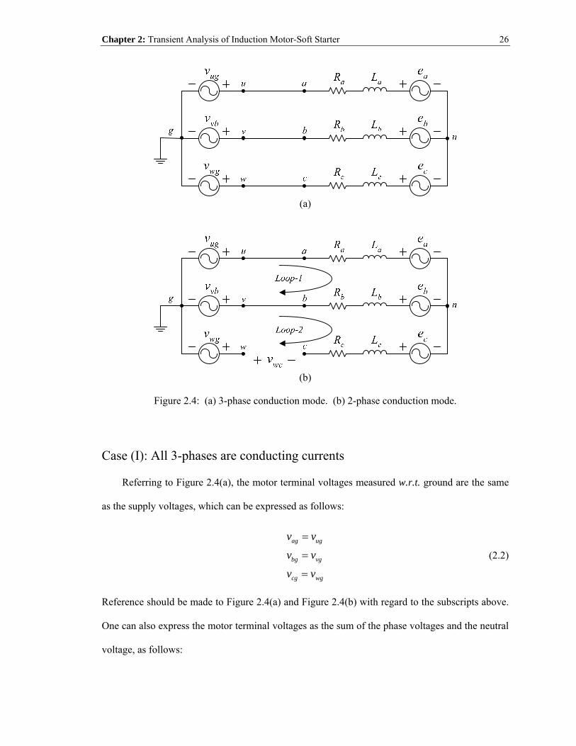
Chapter 2: Transient Analysis of Induction Motor-Soft Starter
26
(a)
(b)
Figure 2.4: (a) 3-phase conduction mode. (b) 2-phase conduction mode.
Case (I): All 3-phases are conducting currents
Referring to Figure 2.4(a), the motor terminal voltages measured w.r.t. ground are the same
as the supply voltages, which can be expressed as follows:
ag ug
bg vg
cg wg
v v
v v
v v
=
=
=
(2.2)
Reference should be made to Figure 2.4(a) and Figure 2.4(b) with regard to the subscripts above.
One can also express the motor terminal voltages as the sum of the phase voltages and the neutral
voltage, as follows:

Chapter 2: Transient Analysis of Induction Motor-Soft Starter
27
ag an ng
bg bn ng
cg cn ng
v v v
v v v
v v v
= +
= +
= +
(2.3)
Substituting (2.2) into (2.3), and summing the left-hand and right-hand side of the above
expression yields the following:
3ug vg wg an bn cn ngv v v v v v v+ + = + + + (2.4)
For a balanced 3-phase supply and a balanced motor, 0ug vg wgv v v+ + = and 0an bn cnv v v+ + = ,
which implies 0ngv = . Accordingly, from (2.2) and (2.3), the motor phase voltages are identical
to the supply voltages when all 3-phases are conducting, that is:
an ug
bn vg
cn wg
v v
v v
v v
=
=
=
(2.5)
Case (II): Only 2-phases are conducting currents
As may be observed from Figure 2.4(b), only phase-a and phase-b are conducting currents,
while the SCRs of phase-c are turned-off. Applying Kirchhoff’s Voltage Law in loop-2, the
voltage across the turned-off SCRs of phase-c, wcv , is:
wc wg vg bn cv v v v e= − + − (2.6)
Note that cn cv e= since phase-c is not conducting any current. Applying KVL in loop-1, one
obtains the following:
an bn ug vgv v v v− = − (2.7)
For a balanced 3-phase motor, an bn cn bn cv v v v e= − − = − − . Hence, one can rewrite (2.7), as
follows:

Chapter 2: Transient Analysis of Induction Motor-Soft Starter
28
( )1 2bn vg ug cv v v e= ⋅ − − (2.8)
Substituting (2.8) into (2.6) yields the following:
( )3 2wc wg cv v e= ⋅ − (2.9)
From Figure 2.4(b), the motor phase-c terminal voltage, cgv , can be defined as follows:
cg wg wcv v v= − (2.10)
By substituting (2.9) into (2.10), the motor terminal voltages w.r.t. ground, when only phase-a
and phase-b are conducting, can be expressed in terms of the supply voltages and motor back
EMF, as follows:
( ) ( )1 2 3 2
ag ug
bg vg
cg wg c
v v
v v
v v e
=
=
= − +
(2.11)
Similarly, when only phase-a and phase-c are conducting, one can write:
( ) ( )1 2 3 2ag ug
bg vg b
cg wg
v v
v v e
v v
=
= − +
=
(2.12)
and when only phase-b and phase-c are conducting, one can write:
( ) ( )1 2 3 2ag ug a
bg vg
cg wg
v v e
v v
v v
= − +
=
=
(2.13)
In order to acquire the motor phase voltages, one can use (2.3) along with the fact that
1 3 ( )ng ag bg cgv v v v= ⋅ + + to obtain the following expression:

Chapter 2: Transient Analysis of Induction Motor-Soft Starter
29
2 3 1 3 1 31 3 2 3 1 31 3 1 3 2 3
an ag
bn bg
cn cg
v vv vv v
⎡ ⎤− −⎡ ⎤ ⎡ ⎤⎢ ⎥⎢ ⎥ ⎢ ⎥= − − ⋅ ⎢ ⎥⎢ ⎥ ⎢ ⎥⎢ ⎥⎢ ⎥ ⎢ ⎥− −⎣ ⎦ ⎣ ⎦ ⎣ ⎦
(2.14)
Using (2.11) through (2.14), the motor phase voltages under 2-phase conduction mode for all
cases can be evaluated, as follows:
For phase-a and phase-b conduction only,
( )( )
1 2
1 2
an ug vg c
bn vg ug c
cn c
v v v e
v v v e
v e
= ⋅ − −
= ⋅ − −
=
(2.15)
and for phase-b and phase-c conduction only,
( )( )
1 2
1 2
an a
bn vg wg a
cn wg vg a
v e
v v v e
v v v e
=
= ⋅ − −
= ⋅ − −
(2.16)
and for phase-a and phase-c conduction only,
( )
( )
1 2
1 2
an ug wg b
bn b
cn wg ug b
v v v e
v e
v v v e
= ⋅ − −
=
= ⋅ − −
(2.17)
Notice that these phase voltages are expressed in terms of only the supply voltages and the back
EMFs, which are presumably known quantities.
A typical healthy transient current space-vector polar plot during soft starting is shown in
Figure 2.5. As one may observe, there are 12 distinct switching states (S1-S12) in every complete
ac power cycle. The machine will only produce a resultant rotating stator mmf when all three
phases of the motor are carrying currents. In the event when only two phases are conducting
currents, the resultant stator mmf produced by the motor consist of a forward rotating mmf
component and a backward rotating mmf component of equal magnitudes. This is due to the fact

Chapter 2: Transient Analysis of Induction Motor-Soft Starter
30
iq
id
Figure 2.5: Healthy transient current space-vector plot during soft starting.
Figure 2.6: Healthy transient three-phase currents during soft starting.

Chapter 2: Transient Analysis of Induction Motor-Soft Starter
31
that the current flowing into one phase is the same as the current flowing out of another phase.
Hence, it will display as a straight line, instead of a quasi-circular outward spiraling locus that
follows the transient current built-up, followed by a quasi-circular inward spiraling locus during
the transient current decay to its final steady-state value. The corresponding space-vector plot is
given in Figure 2.5. It should be noted that Figure 2.5 only presents the transient performance of
the motor where the current space-vector is spiraled outwards with increasing speed. A typical
healthy transient three-phase current waveform during soft starting is given in Figure 2.6.
By virtue of the 12 distinct switching states, the motor phase voltages over a complete ac
cycle can be computed using the above derivations given in (2.5) and (2.15) through (2.17). In
light of the half-wave symmetry, the phase-a voltage is expressed here over a half cycle, as
follows:
, ,
1 2 ( ), ,
1 2 ( ), ,
a
ug
ug vg can
ug
ug wg b
ug
e tv
v v ev
vv v e
v
φ ω αα< <⎧
⎪ <⎪⎪ ⋅ − −⎪= ⎨⎪⎪ ⋅ − −⎪⎪⎩
33 33 2 3
2 3 2 32 3
ttttt
ω φ πφ π ω α πα π ω φ πφ π ω α πα π ω φ π
< ++ < < ++ < < ++ < < ++ < < +
(2.18)
For completeness of this work, the phase-b and phase-c voltages are also expressed here over
a half cycle, as follows:
1 2 ( ),, 3
1 2 ( ), 3 3, 3 2 3
, 2,
vg wg a
vg
vg ug cbn
vg
b
vg
v v e tv t
v v e tv
v tev
φ ω αα ω φ πφ π ω α πα π ω φ πφ π
⋅ − − < <⎧⎪ < < +⎪⎪ ⋅ − − + < < +⎪= ⎨ + < < +⎪⎪ +⎪⎪⎩
3 2 32 3
tt
ω α πα π ω φ π
< < ++ < < +
(2.19)

Chapter 2: Transient Analysis of Induction Motor-Soft Starter
32
1 2 ( ),, 3
, 3 3, 3 2 3
1 2 ( ), 2 3 2 3, 2 3
wg vg a
wg
ccn
wg
wg ug b
wg
v v e tv te t
vv t
v v e tv t
φ ω αα ω φ πφ π ω α πα π ω φ πφ π ω α πα π ω φ π
⋅ − − < <⎧⎪ < < +⎪⎪ + < < +⎪= ⎨ + < < +⎪⎪ ⋅ − − + < < +⎪
+ < < +⎪⎩
(2.20)
Neglecting magnetic saturation and core loss effects, an induction motor can be represented
in a T-equivalent circuit model [87], [88], as given in Figure 2.7. During the transient (soft
starting) period, the slip of the motor is close to one. Hence, m rl rL L R sω ω>> + , which
implies that the magnetizing branch of Figure 2.7 can be neglected in the transient analysis. In
other words, the motor currents produce negligible flux in the airgap, and the magnitudes of these
currents are limited mainly by the leakage reactances. Accordingly, during transient analysis, one
can assume negligible induced EMFs in the windings, i.e. 0a b ce e e= = ≈ . Hence, (2.18)
through (2.20) can be further simplified by equating the EMF terms to zero. Now, the motor
phase voltage expressions depend only on the supply voltages, and hence they can be easily
calculated.
A set of healthy three-phase line-to-neutral motor voltage waveforms obtained from the
closed-form solutions of (2.18) through (2.20), at 60φ = and 90α = is depicted in Figure 2.8.
It is important to mention that the waveforms of Figure 2.8 are only valid for transient analysis,
which is the subject of this work, due to the fact that the induced EMF in the windings cannot be
neglected during the steady state operation. Harmonic breakdown of these motor phase voltages
of Figure 2.8, subject to the formulation given in (2.21), are indicated in Table 2.1. The harmonic
frequency components of Table 2.1 correspond to the three-phase motor voltages of a case-study
being considered here under a healthy condition. In Table 2.1, the magnitude corresponds to Vs(h),
and the phase angle corresponds to θv(h), in the formulation of (2.21). This table gives the
magnitudes and phase angles for the a, b, and c motor terminal phase voltages.

Chapter 2: Transient Analysis of Induction Motor-Soft Starter
33
jhω jhω
jhω
Figure 2.7: T-equivalent circuit model (h is the harmonic order).
-500
0
500
-500
0
500
Mot
or P
hase
Vol
tage
s (V
)
0 0.01 0.02 0.03 0.04-500
0
500
Time (sec)
Phase-a
Phase-b
Phase-c
Figure 2.8: Analytical solution of healthy three-phase line-to-neutral motor voltage waveforms at operating conditions of 60φ = and 90α = .
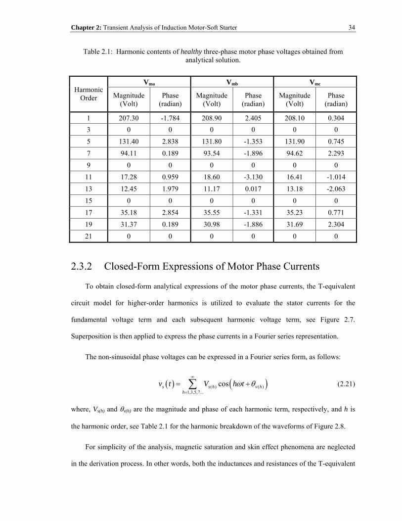
Chapter 2: Transient Analysis of Induction Motor-Soft Starter
34
Table 2.1: Harmonic contents of healthy three-phase motor phase voltages obtained from analytical solution.
Vma Vmb Vmc Harmonic
Order Magnitude (Volt)
Phase (radian)
Magnitude (Volt)
Phase (radian)
Magnitude (Volt)
Phase (radian)
1 207.30 -1.784 208.90 2.405 208.10 0.304 3 0 0 0 0 0 0 5 131.40 2.838 131.80 -1.353 131.90 0.745 7 94.11 0.189 93.54 -1.896 94.62 2.293 9 0 0 0 0 0 0
11 17.28 0.959 18.60 -3.130 16.41 -1.014 13 12.45 1.979 11.17 0.017 13.18 -2.063 15 0 0 0 0 0 0 17 35.18 2.854 35.55 -1.331 35.23 0.771 19 31.37 0.189 30.98 -1.886 31.69 2.304 21 0 0 0 0 0 0
2.3.2 Closed-Form Expressions of Motor Phase Currents
To obtain closed-form analytical expressions of the motor phase currents, the T-equivalent
circuit model for higher-order harmonics is utilized to evaluate the stator currents for the
fundamental voltage term and each subsequent harmonic voltage term, see Figure 2.7.
Superposition is then applied to express the phase currents in a Fourier series representation.
The non-sinusoidal phase voltages can be expressed in a Fourier series form, as follows:
( ) ( )( ) ( )1,3,5,7...
coss s h v hh
v t V h tω θ∞
=
= +∑ (2.21)
where, Vs(h) and θv(h) are the magnitude and phase of each harmonic term, respectively, and h is
the harmonic order, see Table 2.1 for the harmonic breakdown of the waveforms of Figure 2.8.
For simplicity of the analysis, magnetic saturation and skin effect phenomena are neglected
in the derivation process. In other words, both the inductances and resistances of the T-equivalent

Chapter 2: Transient Analysis of Induction Motor-Soft Starter
35
circuit model are assumed to be constant during the transient analysis. Accordingly, from Figure
2.7, the motor phase current for each harmonic voltage term can be expressed in phasor form, as
follows:
( ) ( )( ) ( ) ( )
s h v hs h s h i h
eq
VI I
Zθ
θ∠
= ∠ = (2.22)
where, Zeq is
( ) ( )
( )m r h rl
eq s slr h m rl
jh L R s jh LZ R jh LR s jh L Lω ωω
ω⋅ +
= + ++ ⋅ +
(2.23)
Knowing the magnitude and phase of each current harmonic term from (2.22), the resulting motor
phase currents can be written in Fourier-series time-domain form, as follows:
( ) ( )( ) ( )1,3,5,7...
coss s h i hh
i t I h tω θ∞
=
= +∑ (2.24)
An interesting observation can be drawn with regard to the slip term of the motor for higher-
order time-harmonics, which can be defined as follows:
( )( )
, 1,7,13,19...
5,11,17,23..,
syn r syn
h
syn r syn
h h for hs
for hh h
ω ω ω
ω ω ω
⎧ − =⎪= ⎨ =+⎪⎩ (2.25)
The first expression of (2.25) corresponds to the harmonic components with forward rotating
mmf, while the second expression corresponds to the harmonic components with backward
rotating mmf. Nevertheless, at higher-order time harmonics, the slip, sh, is approaching one, from
which one draws the conclusion that the time-harmonics of motor currents have negligible
magnetizing components, and therefore produce negligible airgap flux and consequently
negligible induced EMFs in the motor windings.
The computed healthy three-phase current waveforms, using (2.22) through (2.25), at
transient operating conditions of 60φ = , 90α = , and a motor speed of 200-r/min are shown in

Chapter 2: Transient Analysis of Induction Motor-Soft Starter
36
Figure 2.9. The reason for choosing these operating conditions is in light of the fact that during
starting, any induction motor is highly inductive. The initial phase displacement angle, φ, between
the phase voltage and current can be calculated according to (2.23) by setting the slip equal to one
and computing the angle of the complex impedance, Zeq. For this particular 2-hp induction motor
under investigation (see Appendix A for motor specifications), the initial phase angle was
calculated to be about 60 . Hence this phase angle, 60φ = , is chosen and kept constant
throughout the analysis process for simplicity’s reason. As for choosing 90α = and a speed of
200-r/min, this is to compare and help validate the analytical results by comparison with the
simulation results at this particular time instant during the transient period of the simulation,
which will be presented later-on in this dissertation. Harmonic contents of these three-phase
motor currents of Figure 2.9 are given in Table 2.2.
To further demonstrate the usefulness of the derived closed-form solution, the RMS values
of the healthy three-phase currents during the soft starting transient are computed and presented
in Table 2.3. In this work, an alpha angle of 105α = was chosen as the initial delay/firing angle.
This delay angle gradually decreases as the motor speeds up until a final delay angle of 65α =
is reached. At this point, the RMS values of the currents can no longer be computed from the
closed-form expressions owing to the fact that the phase angle, φ , is set at 60 during the
computation process. Nevertheless, the analytical results of Table 2.3 demonstrate that the three-
phase currents are balanced during the starting transient with reduced RMS values. It will be
shown later in the simulation chapter that the analytical results begin to deviate from the
simulations as the currents are approaching their rated values. This is due to the fact that the
induction motor is no longer highly inductive as the motor is approaching its rated speed.
Therefore, the phase angle, φ , is approaching the power factor angle in the simulations, whereas
this angle is kept constant at 60 in the closed-form solution. Another reason is due to the

Chapter 2: Transient Analysis of Induction Motor-Soft Starter
37
0.3 0.31 0.32 0.33 0.34 0.35-20
-15
-10
-5
0
5
10
15
20
Mot
or C
urre
nts (
A)
Time (sec)
IaIbIc
Figure 2.9: Analytical solution of healthy three-phase current waveforms at transient conditions of 60φ = , 90α = , and motor speed of 200-r/min.
Table 2.2: Harmonic contents of healthy three-phase motor currents obtained from analytical solution.
Ima Imb Imc Harmonic
Order Magnitude (Amp)
Phase (radian)
Magnitude (Amp)
Phase (radian)
Magnitude (Amp)
Phase (radian)
1 14.255 -2.869 14.340 1.320 14.326 -0.781 3 0 0 0 0 0 0 5 2.021 1.364 2.027 -2.827 2.028 -0.729 7 1.036 -1.313 1.030 2.886 1.042 0.791 9 0 0 0 0 0 0
11 0.121 -0.568 0.131 1.626 0.115 -2.541 13 0.074 0.445 0.066 -1.516 0.078 2.686 15 0 0 0 0 0 0 17 0.160 1.312 0.162 -2.873 0.160 -0.772 19 0.128 -1.357 0.126 2.852 0.129 0.759 21 0 0 0 0 0 0

Chapter 2: Transient Analysis of Induction Motor-Soft Starter
38
Table 2.3: Analytical solution of RMS values of healthy three-phase stator currents during the soft starting transient period.
α-Firing Angle (degree)
Ima RMS value
(Amp)
Imb RMS value
(Amp)
Imc RMS value
(Amp)
105 5.75 5.76 5.70 100 7.25 7.24 7.20 95 8.75 8.73 8.69 90 10.08 10.14 10.13 85 11.47 11.52 11.53 80 12.76 12.80 12.82 75 13.82 13.85 13.88 70 14.40 14.40 14.45 65 13.54 13.53 13.58
assumption that the induced EMFs in the windings are negligible in the closed-form analysis,
which is no longer valid as the motor is approaching its rated speed. Nevertheless, the objective
of this work is to analyze the motor transient performance during soft starting. Therefore, the
analytical results presented in Figure 2.9 and Table 2.3 are acceptable for this stage of the work.
2.4 Analysis of Failure Modes and Effects
The earlier formulations of the closed-form analytical expressions of the motor phase
voltages and currents are employed herein to investigate the impact of failure modes in soft
starters on the motor transient performance. Two distinct types of failure modes considered in this
work are: (1) short-circuit SCR fault (see Figure 2.10(a)), and (2) open-circuit SCR fault (see
Figure 2.10(b)), occurring only in one phase of the soft starter. A short-circuit SCR fault can
happen in situations such as loose wire in the circuit or breakdown in the snubber circuit.
Conversely, an open-circuit SCR fault can occur due to malfunctions either in the gate driver or
the pulse generator of the controller.
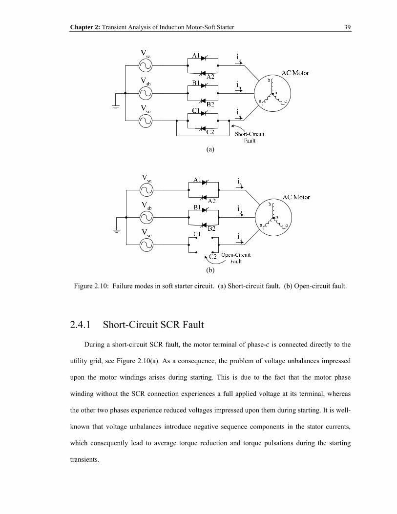
Chapter 2: Transient Analysis of Induction Motor-Soft Starter
39
(a)
(b)
Figure 2.10: Failure modes in soft starter circuit. (a) Short-circuit fault. (b) Open-circuit fault.
2.4.1 Short-Circuit SCR Fault
During a short-circuit SCR fault, the motor terminal of phase-c is connected directly to the
utility grid, see Figure 2.10(a). As a consequence, the problem of voltage unbalances impressed
upon the motor windings arises during starting. This is due to the fact that the motor phase
winding without the SCR connection experiences a full applied voltage at its terminal, whereas
the other two phases experience reduced voltages impressed upon them during starting. It is well-
known that voltage unbalances introduce negative sequence components in the stator currents,
which consequently lead to average torque reduction and torque pulsations during the starting
transients.

Chapter 2: Transient Analysis of Induction Motor-Soft Starter
40
Intuitively, a short-circuit SCR fault is analogous to turning on SCRs C1 and C2
continuously, see Figure 2.10(a). Hence, referring to Figure 2.5, one can deduce that the
switching states, S2-S4, will combine to form one switching state. The same can be said for the
switching states, S8-S10. Accordingly, the 12 switching states under healthy operation will reduce
to 8 switching states under a short-circuit SCR fault. A transient current space-vector polar plot
during soft starting under a short-circuit SCR switch fault is illustrated in Figure 2.11. Notice in
the figure the 8 distinct switching states that were mentioned earlier. Besides that, the shape of the
current space-vector is more elliptic and no longer of circular nature as in the healthy case.
Furthermore, as one can observe, the magnitude of the current space-vector during starting is
higher as compared to the healthy case, see Figure 2.5. Accordingly, this will impose a greater
stress on the motor windings, and consequently higher torque pulsations owing to the higher
starting currents which contain a negative sequence influence.
iq
id
Figure 2.11: Transient current space-vector plot during soft starting under a short-circuit SCR fault.

Chapter 2: Transient Analysis of Induction Motor-Soft Starter
41
Applying the earlier closed-form derivation of the motor line-to-neutral phase voltages with
the switching states of Figure 2.11, the phase-a voltage is expressed here over a half cycle, in
light of the half-wave symmetry, as follows:
,, 2 3
1 2 ( ), 2 3 2 3
, 2 3
a
ugan
ug wg b
ug
e tv t
vv v e t
v t
φ ω αα ω φ πφ π ω α πα π ω φ π
< <⎧⎪ < < +⎪= ⎨ ⋅ − − + < < +⎪⎪ + < < +⎩
(2.26)
Similarly, voltage expressions for phase-b and phase-c can be derived in the same manner,
which are expressed as follows:
1 2 ( ),, 2 3
, 2 3 2 3, 2 3
vg wg a
vgbn
b
vg
v v e tv t
ve tv t
φ ω αα ω φ πφ π ω α πα π ω φ π
⋅ − − < <⎧⎪ < < +⎪= ⎨ + < < +⎪⎪ + < < +⎩
(2.27)
1 2 ( ),, 2 3
1 2 ( ), 2 3 2 3
, 2 3
wg vg a
wgcn
wg ug b
wg
v v e tv t
vv v e t
v t
φ ω αα ω φ πφ π ω α πα π ω φ π
⋅ − − < <⎧⎪ < < +⎪= ⎨ ⋅ − − + < < +⎪⎪ + < < +⎩
(2.28)
The calculated three-phase line-to-neutral motor voltages based on these analytical
expressions of (2.26) through (2.28) are illustrated in Figure 2.12, along with the corresponding
harmonic frequency breakdown of these voltages which are given in Table 2.4. Examination of
Figure 2.12 and Table 2.4 show that the motor voltage waveforms in all phases are
unsymmetrical and unbalanced due to the impact of the short-circuit SCR switch fault in phase-c.
Using the approach described earlier in attaining the analytical expressions of the motor
currents, the calculated three-phase motor currents at transient operating conditions of 60φ = ,
90α = , and a motor speed of 400-r/min are given in Figure 2.13, and the corresponding
harmonic contents of these currents are given in Table 2.5. The analytical results of Figure 2.13

Chapter 2: Transient Analysis of Induction Motor-Soft Starter
42
-500
0
500
-500
0
500M
otor
Pha
se V
olta
ges (
V)
0 0.01 0.02 0.03-500
0
500
Time (sec)
Phase-a
Phase-b
Phase-c
Figure 2.12: Three-phase line-to-neutral motor voltage waveforms from analytical solution under a short-circuit SCR fault.
Table 2.4: Harmonic contents of three-phase motor phase voltages obtained from analytical solution under a short-circuit SCR fault.
Vma Vmb Vmc Harmonic
Order Magnitude (Volt)
Phase (radian)
Magnitude (Volt)
Phase (radian)
Magnitude (Volt)
Phase (radian)
1 259.30 -1.909 220.80 2.678 318.80 0.475 3 54.98 -0.816 52.48 -0.809 107.50 2.329 5 116.60 2.500 116.20 -1.018 43.55 0.733 7 82.65 0.520 82.85 -2.232 32.03 2.279 9 17.12 -2.519 19.23 -2.429 36.30 0.670
11 15.62 0.639 16.70 -2.847 5.64 -0.914 13 10.67 2.332 9.60 -0.395 4.31 -1.926 15 10.88 -0.820 8.60 -0.698 19.44 2.375 17 31.60 2.509 31.24 -0.995 11.32 0.725 19 27.35 0.511 27.55 -2.227 11.01 2.266 21 6.11 -2.592 7.98 -2.402 14.03 0.657
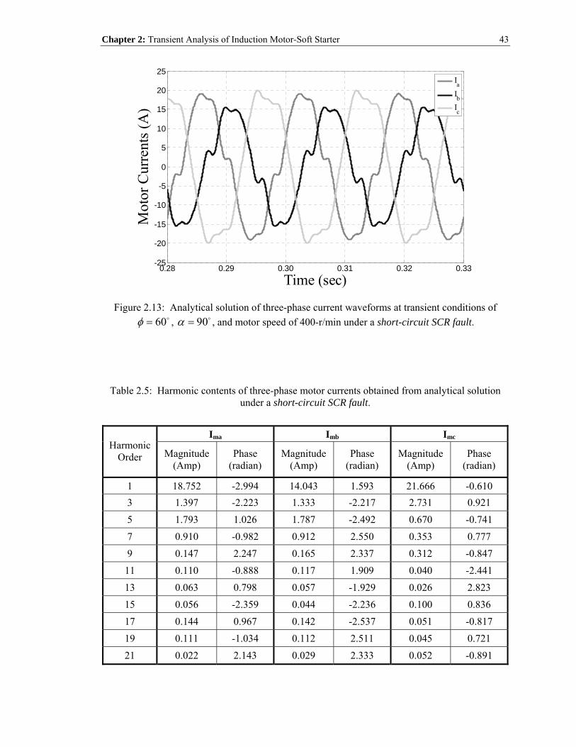
Chapter 2: Transient Analysis of Induction Motor-Soft Starter
43
0.28 0.29 0.30 0.31 0.32 0.33-25
-20
-15
-10
-5
0
5
10
15
20
25
Mot
or C
urre
nts (
A)
Time (sec)
IaIbIc
Figure 2.13: Analytical solution of three-phase current waveforms at transient conditions of 60φ = , 90α = , and motor speed of 400-r/min under a short-circuit SCR fault.
Table 2.5: Harmonic contents of three-phase motor currents obtained from analytical solution under a short-circuit SCR fault.
Ima Imb Imc Harmonic
Order Magnitude (Amp)
Phase (radian)
Magnitude (Amp)
Phase (radian)
Magnitude (Amp)
Phase (radian)
1 18.752 -2.994 14.043 1.593 21.666 -0.610 3 1.397 -2.223 1.333 -2.217 2.731 0.921 5 1.793 1.026 1.787 -2.492 0.670 -0.741 7 0.910 -0.982 0.912 2.550 0.353 0.777 9 0.147 2.247 0.165 2.337 0.312 -0.847
11 0.110 -0.888 0.117 1.909 0.040 -2.441 13 0.063 0.798 0.057 -1.929 0.026 2.823 15 0.056 -2.359 0.044 -2.236 0.100 0.836 17 0.144 0.967 0.142 -2.537 0.051 -0.817 19 0.111 -1.034 0.112 2.511 0.045 0.721 21 0.022 2.143 0.029 2.333 0.052 -0.891

Chapter 2: Transient Analysis of Induction Motor-Soft Starter
44
Table 2.6: Analytical solution of RMS values of three-phase stator currents under a short-circuit SCR fault during the soft starting transient period.
α-Firing Angle (degree)
Ima RMS value
(Amp)
Imb RMS value
(Amp)
Imc RMS value
(Amp)
105 11.41 6.22 13.51 100 12.07 7.47 14.17 95 12.71 8.81 14.82 90 13.26 9.93 15.32 85 13.72 11.04 15.73 80 13.81 11.68 15.81 75 13.01 11.71 15.48 70 10.77 10.21 12.66 65 3.75 4.57 5.14
and Table 2.5 reveal the unbalanced nature of these currents in all phases attributable to the short-
circuit SCR switch fault. The RMS values of the three-phase motor currents during the entire soft
starting period obtained from closed-form solution are tabulated in Table 2.6. Again, it should be
noted that the currents are unbalanced during starting. These unbalanced currents will accordingly
lead to undesired torque reduction and transient torque pulsations, as will be demonstrated
through simulations in later chapters. Comparing Table 2.6 with Table 2.3, one can deduce that
the currents during starting under faulty conditions are higher than in the healthy case.
2.4.2 Open-Circuit SCR Fault
An open-circuit fault in the SCR switches can happen when there is a malfunction in the gate
driver or the controller that prevents gating of the SCR switches. One common type which is
under consideration in this work is depicted in Figure 2.10(b), where both the SCR switches of
one phase are inactive. A fault of this nature results in either 2-phase or 1-phase conduction mode
during soft starting. Clearly, in the event of 1-phase conduction mode, the motor is incapable of
starting since there is no complete path for the current to flow.

Chapter 2: Transient Analysis of Induction Motor-Soft Starter
45
As in the case of 2-phase conduction mode, the current flowing into one phase will be
equivalent to the current flowing out of another phase, that is a bi i= − in Figure 2.10(b). Suppose
that the phase-a and phase-b winding currents of Figure 2.10(b) are:
( ) ( )( ) ( )
cos Amps
cosa m
b m
i t I ti t I t
ωω π
== −
(2.29)
where, Im is the peak amplitude of the winding currents.
Considering only the fundamental space harmonic terms, the mmfs of phase-a and phase-b
can be expressed as follows [88]:
( ) ( )
( ) ( )
1
1
4 cos AT/pole
4 cos 2 3
ph w aa
ph w bb
N k ip m
N k ip m
θ θπ
θ θ ππ
⎛ ⎞⎛ ⎞= ⎜ ⎟⎜ ⎟⎝ ⎠⎝ ⎠
⎛ ⎞⎛ ⎞= −⎜ ⎟⎜ ⎟⎝ ⎠⎝ ⎠
F
F
(2.30)
where, Nph is the effective number of series stator turns per phase, p is the number of poles, m is
the number of parallel paths per phase, and 1wk is the fundamental winding factor.
Accordingly, the fundamental resultant mmf corresponding to the phase-a and phase-b
current excitations of (2.29) can be written as follows:
( ) ( ) ( ) ( ) ( )1 1resultant max, cos cos cos 2 3 cos AT/polet F t tθ θ ω θ π ω π= + − −F (2.31)
where, ( )( )1 1max 4 ph w mF N k mp Iπ= AT/pole.
The resultant mmf of (2.31) can be rewritten by applying the following trigonometric
identity:
( ) ( ) ( ) ( )cos cos 1 2 cos 1 2 cosa b a b a b= ⋅ − + ⋅ + (2.32)
which leads to
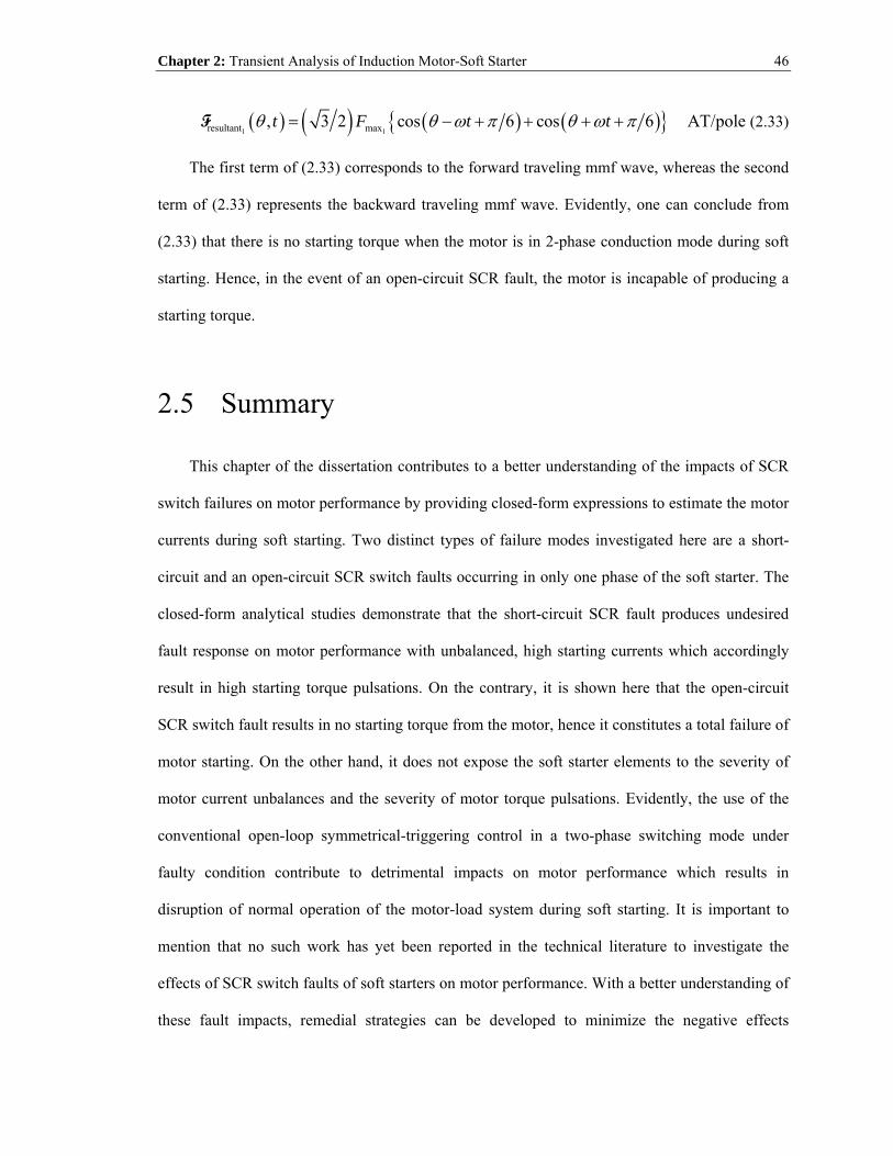
Chapter 2: Transient Analysis of Induction Motor-Soft Starter
46
( ) ( ) ( ) ( )1 1resultant max, 3 2 cos 6 cos 6 AT/polet F t tθ θ ω π θ ω π= − + + + +F (2.33)
The first term of (2.33) corresponds to the forward traveling mmf wave, whereas the second
term of (2.33) represents the backward traveling mmf wave. Evidently, one can conclude from
(2.33) that there is no starting torque when the motor is in 2-phase conduction mode during soft
starting. Hence, in the event of an open-circuit SCR fault, the motor is incapable of producing a
starting torque.
2.5 Summary
This chapter of the dissertation contributes to a better understanding of the impacts of SCR
switch failures on motor performance by providing closed-form expressions to estimate the motor
currents during soft starting. Two distinct types of failure modes investigated here are a short-
circuit and an open-circuit SCR switch faults occurring in only one phase of the soft starter. The
closed-form analytical studies demonstrate that the short-circuit SCR fault produces undesired
fault response on motor performance with unbalanced, high starting currents which accordingly
result in high starting torque pulsations. On the contrary, it is shown here that the open-circuit
SCR switch fault results in no starting torque from the motor, hence it constitutes a total failure of
motor starting. On the other hand, it does not expose the soft starter elements to the severity of
motor current unbalances and the severity of motor torque pulsations. Evidently, the use of the
conventional open-loop symmetrical-triggering control in a two-phase switching mode under
faulty condition contribute to detrimental impacts on motor performance which results in
disruption of normal operation of the motor-load system during soft starting. It is important to
mention that no such work has yet been reported in the technical literature to investigate the
effects of SCR switch faults of soft starters on motor performance. With a better understanding of
these fault impacts, remedial strategies can be developed to minimize the negative effects

Chapter 2: Transient Analysis of Induction Motor-Soft Starter
47
resulting from such faults during normal soft starting operation, which is presented in the
following chapter.

48
CHAPTER 3
3 FAULT TOLERANT SOFT STARTER
3.1 Introduction
As demonstrated in the preceding chapter, the use of the conventional open-loop
symmetrical-triggering control of the soft starter in two-phase switching mode, under short-circuit
SCR switch fault condition produces undesired impacts on machine performance. This situation
results in unbalanced and unsymmetrical high currents during soft starting. Furthermore, the
conventional soft starter system, such as the commercially available type, is incapable of driving
the motor under open-circuit SCR switch fault condition. Accordingly, the soft starter topology
and its control algorithm need to be tailored in order to render the soft starter fault tolerant under
both open-circuit and short-circuit switch fault conditions in any one of the phases. This is while
still providing reduced starting inrush currents, and consequently reduced starting torque
transients. In this chapter, the fault tolerant soft starter topology and its resilient closed-loop two-
phase control scheme will be set forth. The design procedures of the soft starter controller will
also be presented using small-signal modeling approach.

Chapter 3: Fault Tolerant Soft Starter
49
3.2 Principles of Fault Tolerant Operations
The main concerns in designing and constructing any fault tolerant system are the potential
added cost and feasibility issues. The increased cost of incorporating fault tolerant capabilities
into the existing system should always be compared with the cost of damage to the motor-load
system when functioning with the existing configuration without such fault tolerant capabilities
under faulty conditions. It would not make sense to implement a fault tolerant capability to the
existing technology if the added components and manufacturing costs are higher than either the
cost of having system redundancy, or the cost of damage to the overall system, when operating
under a faulty condition with no remedial action being taken. Hence, a designer should always
take these factors into account when designing a fault tolerant system. In the opinion of this
investigator, the most cost-effective means is to modify the existing control algorithm to
accommodate the impact of a fault while still providing acceptable performance. Such a measure
usually involves hardware modifications which need to be performed in a modest and cost-
effective manner.
In this work, the proposed fault tolerant soft starter system is designed with minimum
hardware modifications to the existing commercially available soft starter. To reiterate, the fault
tolerant feature can be easily incorporated into the existing hardware. The added hardware is
modest and hence does not increase the size of the existing system with only minimum increase
in the component cost. The control algorithm was implemented in a closed-loop form which is
more dynamic, effective, and robust in so far as controllability and performance issues are
concerned. The proposed scheme is simple and can be easily implemented with the digital signal
processing power available in the existing technology. Thus, the proposed controls, along with
minimum modification to the hardware circuit topology, present enticing solutions to industries
for such technology to be adopted and implemented in their existing products for mitigating
Chapter 3: Fault Tolerant Soft Starter
50
detrimental effects resulting from a faulty soft starter. In fact, by adopting the proposed control
technique, a low-cost soft starter with only two-phase switching mode can be developed and
produced in the market for consumers at a lower cost with reasonably good performance, as
compared to the existing three-phase soft starter products.
3.2.1 Modified Topology
The vital part of realizing the fault tolerance of the soft starter through integrating the
proposed control algorithm is the amendment of its hardware configuration. Only two significant
modifications in terms of hardware were made to the industrial type soft starter of Figure 2.1,
which is repeated here for convenience in Figure 3.1. A modified version of the soft starter to
accommodate the proposed control technique is illustrated in Figure 3.2. The first modification is
the addition of a set of three-phase voltage sensors at the motor end of the soft starter to measure
the motor terminal voltages. The reason for having these sensors is that the motor terminal
voltage measurement will be employed as one set of the feedback signals for the present closed-
loop control scheme. The second modification is the replacement of the existing 3-pole
synchronously-controlled modular contactor with three individually-controlled 1-pole contactors,
one pole per phase. The main purpose of this modification is such that the contactor of the
corresponding SCR phase can be closed in the event of an open-circuit SCR switch fault. This is
in order to isolate the faulty SCR phase, as depicted in Figure 3.3. Accordingly, the soft starter
can function in a two-phase switching mode using the present two-phase control approach. In the
event of a short-circuit SCR fault, the corresponding motor phase is automatically connected
directly to the utility mains, and hence the soft starter is already in its two-phase switching mode.
As one can see from the desired hardware modifications to the industrial type soft starter, the
suggested changes barely increase the size of the existing system with only minor increase in the
component cost. Such design modifications with minimum cost increase are usually acceptable
within industrial practice. Due to the asymmetry of the post-fault two-phase thyristors configura-

Chapter 3: Fault Tolerant Soft Starter
51
a
b
cn
AC Motor
iaVsa
Vsb
Vsc
ib
ic
SourceVoltages
andLine Currents
Zero-CrossingDetection
+Controller
GatePulses
A 3-PoleSynchronously-Controlled
Modular Contactor
Sensors
Figure 3.1: Industrial type three-phase soft starter topology.
Figure 3.2: Modified version of soft starter with fault tolerance/isolation capabilities.

Chapter 3: Fault Tolerant Soft Starter
52
Figure 3.3: Post-fault soft starter configuration.
-tion shown in Figure 3.3, the problem of voltage unbalances impressed upon the motor windings
arises during starting. This is due to the fact that the motor phase winding without the SCR
connection experiences a full applied voltage, whereas the other two phases experience reduced
voltages impressed upon them during starting. It is well-known that voltage unbalances introduce
negative sequence components in the stator currents, which consequently lead to torque
pulsations during the starting transients. Therefore, the control strategy has to be tailored to
control the firing of the thyristors in the remaining two phases independently. This is in order to
generate nearly balanced three-phase stator currents during the soft starting period, so that the
starting torque pulsations can be alleviated. Hence, a closed-loop type of control is adopted which
is presented next.
3.2.2 A Resilient Closed-Loop Two-Phase Control Scheme
In order to control the firing of the thyristors in the remaining two healthy phases
independently, a new set of firing angles for each of the two phases has to be defined. Such a task

Chapter 3: Fault Tolerant Soft Starter
53
is not easy to achieve using open-loop control, since the firing angle profile will vary with
different horsepower motors as well as load conditions. Therefore, closed-loop type of control
was adopted here, which will inherently generate the appropriate firing angle profile for the
thyristors of each of the two phases under different horsepower motor ratings and different types
of load conditions.
The present closed-loop two-phase control scheme is graphically depicted in Figure 3.4 for
the post-fault soft starter configuration of Figure 3.3. In this control method, there are two types
of feedback control loops, namely a voltage loop and a current loop for each of the remaining two
healthy phases. The outputs of these feedback loops represent the changes in the firing angles that
will be used to compute the resulting firing (delay) angles, which is defined as follows:
0 V I
0 V I
a a a a
b b b b
α α α αα α α α
= − −= − −
(3.1)
where, Vaα and Vbα are the outputs of the voltage feedback loop, Iaα and Ibα are the outputs of
the current feedback loop, and 0aα and 0bα are the initial firing (delay) angles for phase-a and
phase-b, respectively. The resulting firing (delay) angles, aα and bα computed from (3.1) are
used to generate the gate pulses for triggering the thyristors of the two controlled phases. It is of
importance to mention that the α-control approach [29] is adopted here in lieu of the γ-control
approach [23]. This is due to the fact that the motor phase currents are unbalanced and
unsymmetrical during the starting transient period, as was discussed in the preceding chapter.
Consequently, the zero crossings of the currents will accordingly vary in all three phases.
Therefore, the control response will become unstable if the γ-control method, which is dependent
on the zero crossings of the line currents, is adopted. On the other hand, the zero crossings of the
ac mains voltages are symmetrical and phase-shifted by 120 e from each other in all three
phases, regardless of both the conditions of the soft starter and the electric motor. Hence, the α-

Chapter 3: Fault Tolerant Soft Starter
54
Va(rms)
Vramp* VoltagePI
Vb(rms)
Ia(rms)
Ib(rms)
Ic(rms)
VoltagePI
+ 13
Ia(rms)
CurrentPI
Ib(rms)
CurrentPI
Iav*
+-
+-
+-
+-
+--
+--
aα
bα
0aα
0bα
Vaα
Vbα
Iaα
Ibα
Figure 3.4: Present closed-loop two-phase control for fault tolerant soft starter.
Figure 3.5: Reference voltage ramp profile.

Chapter 3: Fault Tolerant Soft Starter
55
control approach, which relies on the zero crossings of the mains voltages, provides a much more
stable control response and thus it is employed in the present control approach.
The voltage feedback loop is used to control the starting acceleration profiles of the motor
currents and torque. It controls the duration of the starting period which varies for different types
of applications. A user-selected voltage ramp profile, Vramp*, is used as a reference command, as
shown in Figure 3.5. It consists of an initial voltage setting, a final voltage setting, and a soft start
(ramp) time setting. The user presets the initial phase voltage percentage that will be impressed
upon the motor windings during the start-up process. Typically, a heavier load which requires a
higher starting torque will need a higher initial impressed voltage. The final voltage setting will
typically be the rated phase voltage of the motor. In addition, the soft start (ramp) time setting
will determine the duration of the starting period before the motor establishes its rated speed. This
voltage ramp profile, Vramp*, is analogous to the user-setting being utilized in industrial-type soft
starters, where the user presets the initial locked rotor torque percentage and the soft start (ramp)
time [31]-[33]. Once the voltage ramp profile, Vramp*, has been predefined during the start-up
process, the effective (rms) values of the measured motor terminal voltages for the two controlled
phases, Va(rms) and Vb(rms), are computed online during the motor starting transients. These values
are then compared with the voltage reference profile, Vramp*, and the errors are conditioned by a
set of voltage Proportional-Integral (PI) regulators. The outputs of the PI regulators represent the
first part of the firing (delay) angles, Vaα and Vbα , see (3.1), for phase-a and phase-b firing
(delay) angles, aα and bα , respectively.
With only the voltage feedback loop, the motor will still exhibit unbalanced starting currents,
and consequently significant starting torque pulsations. Accordingly, in order to ensure nearly
balanced three-phase motor currents during starting, a current feedback loop is utilized, see
Figure 3.4. The effective (rms) values of the three-phase motor currents, Ia(rms), Ib(rms), and Ic(rms),

Chapter 3: Fault Tolerant Soft Starter
56
are measured and the average value of these currents, Iav*, is used as the current reference
command for the current controller, which is expressed as follows:
(rms) (rms) (rms)av
I I II
3a b c∗ + +
= (3.2)
The average current, Iav*, is compared with the measured effective (rms) motor currents of the
two controlled phases, Ia(rms) and Ib(rms), and the errors are conditioned by a set of current PI
regulators. Here, the outputs of the PI regulators represent the second part of the firing angles,
Iaα and Ibα , for phase-a and phase-b firing angles, aα and bα , respectively, see (3.1). By
regulating the rms values of the two controlled phase currents, Ia(rms) and Ib(rms), to be near the
average current value, Iav*, the rms value of the third phase current, Ic(rms), is automatically
adjusted to be the average current, Iav*, so as to satisfy the condition of (3.2). As a result, a nearly
balanced three-phase current condition is realized through this approach, which will in turn
provide reduced starting torque transients. Meanwhile, in order to start up the motor from zero
speed, an initial firing angle for each of the two controlled phases is commanded and is
represented in Figure 3.4 as 0aα and 0bα . The final firing (delay) angle profiles for the two-
phase control for triggering the two-phase thyristors are defined as given in (3.1).
3.3 Small-Signal Modeling of Motor-Soft Starter Controller
In this section, a small-signal model representing the motor-soft starter controller is
developed. More specifically, the derivations of the open-loop and closed-loop (feedback) system
transfer functions of the small-signal model consisting of the controller and the plant (induction
motor + soft starter) are detailed here. A simplified control system representing the motor-soft
starter of Figure 3.3, as well as the control algorithm of Figure 3.4 is shown here in Figure 3.6. It

Chapter 3: Fault Tolerant Soft Starter
57
consists of the transfer function of the plant, Gp(s), the transfer function of the controller, Gc(s),
the reference inputs, I(s)* and V(s)*, and the system outputs, I(s) and V(s). The plant is composed
of a soft starter and an induction motor. Since the soft starter is a nonlinear electrical system, it is
represented here by a nonlinear expression: ( )rmsV f α= , the derivation of which will be
discussed in detail later on in this section. As for the induction motor, a simplified transfer
function of it is also derived and presented here. On the other hand, the controller consists of a set
of PI regulators for the voltage and current loops with unity feedback. It is the reason of tuning
the PI regulators that the small-signal model of Figure 3.6 is being developed and analyzed for
transient response and stability purposes.
As one may observe from the control system of Figure 3.6, there are two feedback loops,
namely the voltage and current loops, which are operating in a parallel fashion. As was
mentioned earlier, these two feedback loops serve different purposes. The voltage loop is
responsible for the starting acceleration of the motor, while the current feedback loop is
accountable for mitigating the unbalanced effects of the starting currents under thyristor switch
fault condition. As a consequence, these two feedback loops are independent of one another, and
hence the control feedback loop of each can be designed in an individual manner. Nevertheless,
the motor can still function with only one feedback loop available, but at a much inferior
performance such as having starting torque pulsations. Therefore, in designing the controller of
Figure 3.6, the control system can be segregated into two separate individual control systems
accountable for the voltage and current loops, as illustrated in Figure 3.7 and Figure 3.8,
respectively. In doing so, the process of designing both the voltage and current regulators is
simplified with only a single input and a single output in the control systems of both Figure 3.7
and Figure 3.8.
Upon observation of the voltage control loop as depicted in Figure 3.7, the plant of this
voltage control system is now represented by the soft starter. This is due to the fact that the main

Chapter 3: Fault Tolerant Soft Starter
58
( )rmsV f α=
Iα
Vα
0 V Iα α α α= − −
Figure 3.6: Simplified control system representation of motor-soft starter controller.
( )αfVrms =_ V
_ Vi
p
kk
s+
Vα
kα
Figure 3.7: Voltage control loop.
( )αfVrms =_ I
_ Ii
p
kk
s+
1
s sr s Lσ+Iα
kα
Figure 3.8: Current control loop.

Chapter 3: Fault Tolerant Soft Starter
59
thrust of the soft starter is to provide voltage excitation, which is dependent on the firing/delay
angle profile, to the motor. Due to its nonlinear nature, the plant (or soft starter) is represented by
a nonlinear expression: ( )rmsV f α= . Meanwhile, the controller consists of only the voltage PI
regulator with a unity voltage feedback loop. On the other hand, in the current control system as
shown in Figure 3.8, the plant consists of both the soft starter and the motor, and the controller is
now a current PI regulator with a unity current feedback loop. The details of derivation of the
corresponding small-signal models are set forth next.
3.3.1 Transfer Function of Controller
The transfer function of the PI controller is straightforward, and it is defined for the voltage
and current loops, Gc_V(s) and Gc_I(s), respectively, as follows:
_ V_ V _ V( ) i
c p
kG s k
s= + (3.3)
_ I_ I _ I( ) i
c p
kG s k
s= + (3.4)
where, kp_V and kp_I are the proportional gains, and ki_V and ki_I are the integral gains of the voltage
and current controllers, respectively.
Owing to the separate control loop for the voltage and current controllers, the corresponding
kp and ki can be easily designed to achieve the selected bandwidth at the crossover frequency
where the gain of the open-loop transfer function equals unity using linear control theory. The
design procedures are detailed in the coming section.
3.3.2 Transfer Function of Induction Motor
In an induction motor, the set of differential equations in dq representation that govern the
instantaneous relationship between the voltages and currents in the synchronously rotating frame
of reference can be expressed in the following manner [87]:

Chapter 3: Fault Tolerant Soft Starter
60
( )
( )
0
0
eqse e e
qs s qs e ds
ee e edsds s ds e qs
eqre e
r qr e r dr
ee edr
r dr e r qr
dv r i
dtdv r idt
dr i
dtdr idt
λω λ
λ ω λ
λω ω λ
λ ω ω λ
= + +
= + −
= + + −
= + − −
(3.5)
where,
e e eqs s qs m qr
e e eds s ds m dr
e e eqr r qr m qs
e e edr r dr m ds
L i L i
L i L i
L i L i
L i L i
λ
λ
λ
λ
= +
= +
= +
= +
(3.6)
Here, s ls mL L L= + and r lr mL L L= + , where, lsL is the stator phase leakage inductance, lrL is
the referred rotor phase leakage inductance, and mL is the magnetizing inductance in the T-
equivalent circuit of an induction machine [88]. The first two equations of (3.5) correspond to the
dq stator windings, while the last two equations of (3.5) correspond to the dq rotor windings. The
equations of (3.6) represent the dq stator and rotor flux linkages. Meanwhile, the terms, eω and
rω , denote the synchronous speed and the rotor speed in electrical radians/second, respectively.
The superscript e indicates the synchronously rotating reference frame.
Under a balanced sinusoidal condition, the “synthetic” dq windings in the synchronously
rotating reference frame will rotate at the same speed as the airgap magnetic field distribution.
Hence, this results in a dc value representation of all the currents, voltages, and flux linkages
associated with the dq stator and rotor windings (note that slip e rω ω ω= − ). Accordingly, this
makes the design process of the PI regulator a much easier task than designing using other
reference frames.

Chapter 3: Fault Tolerant Soft Starter
61
From (3.6), one can rewrite the dq rotor winding currents from the dq rotor winding flux
linkage terms, as follows:
e eqr m qse
qrr
e ee dr m dsdr
r
L ii
L
L iiL
λ
λ
−=
−=
(3.7)
By substituting (3.7), as well as the dq stator winding flux linkage terms of (3.6) into the dq
stator winding voltage expressions of (3.5), one obtains the following [89]:
2 2
Compensation/Decoupling Terms
2
'
'
e e e e e em m m mqs s qs s qs qr e dr s ds
r r r r
v
e e emds s ds s ds
r
v
eqs
eds
L L L Ld dv r i L i L idt L dt L L L
Ldv r i L idt L
λ ω λ⎡ ⎤ ⎡ ⎤⎛ ⎞ ⎛ ⎞ ⎛ ⎞
= + − + + + −⎢ ⎥ ⎢ ⎥⎜ ⎟ ⎜ ⎟ ⎜ ⎟⎝ ⎠ ⎝ ⎠ ⎝ ⎠⎣ ⎦ ⎣ ⎦
⎡ ⎤⎛ ⎞= + −⎢ ⎥⎜ ⎟
⎝ ⎠⎣ ⎦
2
Compensation/Decoupling Terms
e e em m mdr e qr s qs
r r r
L L Ld L idt L L L
λ ω λ⎡ ⎤⎛ ⎞ ⎛ ⎞
+ − + −⎢ ⎥⎜ ⎟ ⎜ ⎟⎝ ⎠ ⎝ ⎠⎣ ⎦
(3.8)
In the q-axis voltage equation of (3.8), only the first two terms on the right hand side are due to
the q-axis current, eqsi . The next two terms of the same equation can be considered as the
compensation or decoupling terms [89]. The same can be stated for the d-axis voltage equation.
Assuming the compensation or decoupling effect is perfect, the new dq-axis voltage
equations can be expressed as follows [89]:
'
'
eqse e
qs s qs s
ee e dsds s ds s
div r i L
dtdiv r i Ldt
σ
σ
= +
= +
(3.9)
where, 21 m s rL L Lσ = − . Hence, the induction motor (plant) can be simply represented by the
above equation as defined in (3.9). The resulting voltage space vector, sv , can therefore be
written in the following manner:

Chapter 3: Fault Tolerant Soft Starter
62
' 'e e ss qs ds s s s
div v jv r i Ldt
σ= + = + (3.10)
Accordingly, a per-phase motor model can be represented by the transfer function block diagram
as depicted in Figure 3.9.
1s1
s sr s Lσ+
1
sLσ
sr
Figure 3.9: Transfer function of per-phase induction motor model.
3.3.3 Nonlinear Representation of Soft Starter
In order to incorporate the electrical behavior of a soft starter into the small-signal model
representing the control system of Figure 3.6, a mathematical expression describing the nonlinear
nature of the soft starter is derived and detailed here. The main thrust of the soft starter is to
provide voltage excitation to the motor, where the rms value of this impressed voltage is
dependent on the firing angle profile. Meanwhile, as one can see from Figure 3.6, the outputs of
the voltage and current PI controllers yield Vα and Iα , respectively. This results in the firing
angles, 0 Vα α α= − and 0 Iα α α= − for the voltage and current PI controllers, respectively,
where 0α denotes the initial firing angle. As a result, a mathematical expression which describes
the relationship between the impressed rms voltage and the firing angle is developed here.
The closed-form expression of the motor line-to-neutral voltage was derived in the
previous chapter and is given here in the following expression for phase-a over a complete cycle:

Chapter 3: Fault Tolerant Soft Starter
63
,, 3
1 2 ( ), 3 3, 3 2 3
1 2 ( ), 2 3 2 3, 2 3
,, 4 3
1 2 ( ), 4 3,
1 2 ( ),,
a
ug
ug vg c
ug
ug wg b
ugan
a
ug
ug vg c
ug
ug wg b
ug
e tv t
v v e tv t
v v e tv t
ve tv t
v v e tv
v v ev
φ ω αα ω φ πφ π ω α πα π ω φ πφ π ω α πα π ω φ πφ π ω α πα π ω φ πφ π ω α
< << < +
⋅ − − + < < ++ < < +
⋅ − − + < < ++ < < +
=+ < < ++ < < +
⋅ − − + < < +
⋅ − −
4 34 3 5 35 3 5 35 3 2
ttt
πα π ω φ πφ π ω α πα π ω φ π
⎧⎪⎪⎪⎪⎪⎪⎪⎪⎨⎪⎪⎪⎪⎪ + < < +⎪
+ < < +⎪⎪ + < < +⎩
(3.11)
where, the induced back emfs, 0a b ce e e= = ≈ during the soft starting transients, and vug, vvg,
and vwg represent the ac mains voltages, which are expressed as follows:
( ) ( )( ) ( )( ) ( )
cos
cos 2 3
cos 4 3
ug m
vg m
wg m
v t V t
v t V t
v t V t
ω
ω π
ω π
=
= −
= −
(3.12)
Accordingly, from the above equations of (3.11) and (3.12), the rms value of the phase-a
voltage, Vrms, can be computed using the following expression:
2 21
2rms anV v dφ π
φθ
π+
= ∫ (3.13)
After performing the necessary mathematical steps, the resulting Vrms can be expressed by the
following nonlinear expression:
( ) ( )3 3 3 3sin 2 sin 22 2 4 42
mrms
VV π φ α α φπ
= + − + − (3.14)
Examination of (3.14) reveals that the only variable is the angle, α , since Vm represents the peak
magnitude of the ac mains voltage (in this case, Vm = 2 265× Volt) and φ is chosen to be 60

Chapter 3: Fault Tolerant Soft Starter
64
(or 3 radπ ) during the soft starting transients, as was mentioned earlier in the preceding
chapter. It should also be noted that by selecting 0 120α = along with the fact that the α
firing/delay angle ranges from 60 to 120 during the starting transients, this results in Vα and
Iα ranging from 0 to 60 . A plot of the motor phase voltage (rms) versus Vα from 0 to 60
using (3.14) is depicted in Figure 3.10. As one can notice from Figure 3.10, at the point of
V 60α φ= = , the SCRs are fully on, which entails the rms voltage value of 265 Vrms for a line-
to-line utility voltage of 460 Vrms.
Despite the nonlinear nature of the soft starter, a linear relationship between the rms motor
phase voltage and the firing angle can be approximately realized at a selected operating point
which results in: VrmsV kαα= and IrmsV kαα= , for the voltage and current loops, respectively,
see Figure 3.7 and Figure 3.8. It should be emphasized that the units of Vα and Iα are in radians
per second when computing the gain kα . Such linearization simplifies the design process in such
a way that linear control systems theory can be employed. Here, Vα and Iα are assumed to have
the same operating point. In this design process, an operating point is chosen where
V I 30 or 6 radα α π= = . Hence, the constant kα can be calculated using (3.14). As a result,
the linear transfer function of the soft starter at the chosen operating point can be approximately
expressed for the voltage and current loops, respectively, as follows:
( )( )( )( )
V
I
rms
rms
V sk
s
V sk
s
α
α
α
α
=
=
(3.15)

Chapter 3: Fault Tolerant Soft Starter
65
0 10 20 30 40 50 6050
100
150
200
250
300
AlphaV (degree)
Vrm
s (Vol
t)
265 Volt (rms)
Figure 3.10: A plot of motor phase voltage (rms) versus αV using Equation (3.14).
3.3.4 Small-Signal Model Representation of Overall System
From the previously derived transfer function of each individual subsystem of Figure 3.6, a
small-signal model of the voltage and current control loops can thus be developed. More
specifically, the open-loop and closed-loop transfer functions of the voltage and current control
loops are derived.
For the voltage control loop of Figure 3.7, the open-loop, ( )_ VOLG s , and the closed-loop,
( )_ VCLG s , transfer functions can be written as follows:
( ) ( ) ( ) ( )
( ) ( )
_ V_ V _ V _ V _ V
_ V_ V
_ V1 1
i p iOL c p p
OL p iCL
OL p i
k k k s k kG s G s G s k k
s sG k k s k k
G sG k k s k k
α αα
α α
α α
+⎛ ⎞= = + =⎜ ⎟
⎝ ⎠+
= =+ + +
(3.16)

Chapter 3: Fault Tolerant Soft Starter
66
Meanwhile, for the current control loop of Figure 3.8, the open-loop, ( )_ IOLG s , and the
closed-loop, ( )_ ICLG s , transfer functions can be expressed in the following manner:
( ) ( ) ( ) ( )
( ) ( )
_ I_ I _ I _ I _ I 2
_ I_ I 2
_ I
1
1
i p iOL c p p
s s s s
OL p iCL
OL s s p i
k k k s k kG s G s G s k k
s r s L L s r sG k k s k k
G sG L s r k k s k k
α αα
α α
α α
σ σ
σ
+⎛ ⎞⎛ ⎞= = + =⎜ ⎟⎜ ⎟ + +⎝ ⎠ ⎝ ⎠
+= =
+ + + +
(3.17)
The design procedures for obtaining kp and ki of the voltage and current PI regulators at selected
bandwidth are detailed next.
3.4 Design Procedures of Soft Starter PI Controllers
The overall motor-soft starter system is designed at a desired bandwidth to provide good
dynamic and fast transient responses to any changes in the reference input to the soft starter
controller. Certain design conditions and criteria are assumed here in order to simplify the overall
design process. In addition, since the soft starter is a nonlinear system, a certain operating point is
selected so that the overall system is assumed to be linear around that selected operating point,
thus allowing the basic concepts of linear control theory to be applied. Once the controller has
been designed, the entire system is simulated under large-signal conditions to evaluate the
adequacy, stability, and response of the controller, which will be presented in the following
chapter.
3.4.1 Voltage Control Loop
In selecting the gain constants of the PI controller of the voltage control loop of Figure 3.7,
the following are the design criteria:
• Crossover frequency of ( )_ VOLG s , 500 Hzcf = .

Chapter 3: Fault Tolerant Soft Starter
67
• Phase Margin (PM) of ( )_ VOLG s , 120PMφ = .
The crossover frequency, fc, is defined as the frequency at which the gain of the open-loop
transfer function equals unity, that is ( )_ V 0 dBOLG s = . On the other hand, the phase margin,
PMφ , is defined as the phase angle of the open-loop transfer function that is measured with
respect to 180− at the crossover frequency [90]. For a satisfactory dynamic transient response
without any instabilities or oscillations, the phase margin should be chosen to be greater than 45
[90]. Meanwhile, the bandwidth (BW) of the overall closed-loop feedback system is defined as
the frequency at which the gain of the closed-loop transfer function drops to 3 dB− . In some
practical applications, the bandwidth of the closed-loop feedback system is approximately equal
to the crossover frequency, fc [90]. Hence, for a fast dynamic transient response by the control
system, the bandwidth of the closed-loop system should be high, which indicates that the
crossover frequency of the open-loop system should be designed to be high. In this design work,
the crossover frequency, fc, was selected to be 500 Hz so that the overall bandwidth of the voltage
control loop is high enough to dynamically respond to changes in the reference input voltage.
Based on the aforementioned design criteria, the following two equations at the crossover
frequency can be defined:
( )
( ) ( )
_ V
_ V
1
rad
cc
c
c
p iOL s j
s j
p iOL PMs j
s j
k k s k kG s
s
k k s k kG s
s
α α
ωω
α α
ωω
π φ
==
==
+= =
+⎛ ⎞∠ = ∠ = − +⎜ ⎟
⎝ ⎠
(3.18)
where, 2c cfω π= is the angular crossover frequency in rad/sec. By solving these two equations
above, one can acquire the gain constants, kp and ki, of the voltage control loop at the selected
design conditions as given in the following expressions:

Chapter 3: Fault Tolerant Soft Starter
68
12
32
p
ci
kk
kk
α
α
ω
=
= (3.19)
As discussed in earlier sections, the gain kα which represents the linear transfer function
gain of the soft starter is computed at a selected operating point with the following conditions:
0 V 120 30 90α α α= − = − = or 2 radπ , 60φ = or 3 radπ , and 2 265 VoltmV = × .
Accordingly, the gain kα was calculated from (3.14) and (3.15), resulting in a value, 374kα ≈ .
With this gain, knowing that 2 2 500 rad/secc cfω π π= = × , the PI gain constants of the voltage
control loop were calculated and found to be: 0.0013pk ≈ and 7.27ik ≈ .
Using the computed gain constants of the voltage PI controller, the corresponding bode plots
of the open-loop and closed-loop transfer functions of the voltage control loop system are
depicted in Figure 3.11(a) and Figure 3.11(b), respectively. As one can observe from Figure
3.11(a), the desired crossover frequency, fc, and the phase margin, PMφ , have been achieved,
according to the design criteria, at 500 Hz and 120 , respectively. The subsequent bandwidth
(BW) of the voltage control loop system of Figure 3.7 was found to be 325 Hz, as indicated in
Figure 3.11(b). This bandwidth is adequately enough for the soft starter to respond to any
variations in the reference input voltage profile. It should also be noticed from Figure 3.11(b) that
the gain of the voltage control loop system is at its maximum, that is ( )_ V 0 dBCLG s = , within
its bandwidth.
3.4.2 Current Control Loop
The current control loop of Figure 3.8 was designed in a similar manner to the voltage
control loop. The following are the design criteria:

Chapter 3: Fault Tolerant Soft Starter
69
-40
-20
0
20
40
60
80
Gai
n (d
B)
Frequency (Hz)10-1 100 101 102 103 104
-90
-45
0
Phas
e (d
eg)
(a)
-10
-8
-6
-4
-2
0
Gai
n (d
B)
10-1 100 101 102 103 104
-90
-45
0
Phas
e (d
eg)
Frequency (Hz) (b)
Figure 3.11: Bode plot of voltage control feedback loop system. (a) Open-loop transfer function. (b) Closed-loop transfer function.

Chapter 3: Fault Tolerant Soft Starter
70
• Crossover frequency of ( )_ IOLG s , 500 Hzcf = .
• Phase Margin (PM) of ( )_ IOLG s , 90PMφ = .
The open-loop transfer function of the current control feedback loop, which is given earlier
in (3.17), is written here, as follows:
( ) ( ) ( ) ( )_ I _ I _ Ip i
OL c ps s
k k s k kG s G s G s
s L s rα α
σ+
= =+
(3.20)
To select the gain constants of the PI controller in the current control loop, a simple design
procedure, which results in a phase margin of 90 as stated above in the design criteria, was
implemented as follows:
Step (1): Select the zero of (3.20) to cancel its corresponding pole.
Under this condition,
1 i
p e ip e
k k kk
στστ
= ⇒ = (3.21)
where, e s sL rτ = is the electrical time constants. This consequently results in the following
transfer function:
( )_ Ii s
OLk k rG s
sα= (3.22)
Examination of (3.22) indicates that the phase margin, PMφ , is 90 which satisfies the above
given design criteria.
Step (2): Compute the crossover frequency such that ( )_ I 1c
c
i sOL s j
s j
k k rG ss
αω
ω=
=
= = .
This yields c i sk k rαω = . Using this equation along with (3.21), one can solve for the PI gain
constants of the current control feedback loop of Figure 3.8, which are expressed as follows:

Chapter 3: Fault Tolerant Soft Starter
71
e s cp
s ci
rkk
rkk
α
α
στ ω
ω
=
= (3.23)
Using the same kα as was computed earlier, along with the given machine parameters of the
case-study 2-hp induction motor (see Appendix A), the PI gain constants of the current control
loop were computed to be, 0.3pk ≈ and 32.3ik ≈ .
With the calculated pk and ik of the current PI regulator, the bode plots of the open-loop
and closed-loop transfer functions of the associated current control feedback loop system of
Figure 3.8 are illustrated in Figure 3.12(a) and Figure 3.12(b), respectively. Evidently, from both
the bode plots of the open-loop and closed-loop transfer functions, the crossover frequency, fc,
and the bandwidth (BW) have been realized at 500 Hz, which fulfills the design criteria.
3.5 Summary
Low-cost fault tolerant solution capable of mitigating thyristor open and short-circuit switch
faults for soft starters has been presented in this chapter. Minimum hardware modifications are
required for the existing commercially available soft starter in order for the fault tolerant
operation to be possible. It should be emphasized that such essential modifications do not
significantly increase the cost and size of the existing system. One of the essential changes
involves adding a set of three-phase voltage transducers on the motor end of the soft starter for
acquiring the motor terminal voltages needed for fault tolerant control purposes. The second
hardware modification involves the replacement of the existing 3-pole synchronously-controlled
modular bypass contactor with a set of individually-controlled 1-pole contactors for all three

Chapter 3: Fault Tolerant Soft Starter
72
-40
-20
0
20
40
60
80
Gai
n (d
B)
10-1 100 101 102 103 104
-90
-45
0
Phas
e (d
eg)
Frequency (Hz) (a)
-30
-20
-10
0
Gai
n (d
B)
10-1 100 101 102 103 104
-90
-45
0
Phas
e (d
eg)
Frequency (Hz) (b)
Figure 3.12: Bode plot of current control feedback loop system. (a) Open-loop transfer function. (b) Closed-loop transfer function.

Chapter 3: Fault Tolerant Soft Starter
73
phases. These contactors are used for fault isolation purposes in such a way that the soft starter
can switch into a two-phase switching mode in the event of an SCR switch fault occurring in any
one of the phases. As for the proposed two-phase control approach, two types of feedback control
loops were adopted. Namely, these are the voltage and current feedback loops, respectively. The
voltage feedback control is responsible for the starting acceleration of the motor, while the
current feedback loop is responsible for mitigating the unbalanced effects of the starting currents
under thyristor switch fault condition. In fact, by adopting the proposed control technique, a low-
cost soft starter with only two-phase switching mode can be developed and produced in the
market for consumers at a lower cost with reasonably good performance, as compared to the
existing three-phase soft starter products.
In addition, small-signal modeling of the motor-soft starter controller system was developed.
More specifically, the open-loop and closed-loop transfer functions of the voltage and current
control feedback loop systems were derived. The main thrust of this small-signal modeling
approach is to design the PI regulators in the voltage and current loops so as to achieve the
desired bandwidth to render a good dynamic and fast transient response. Upon designing the PI
controllers, the entire system was simulated under large-signal conditions to evaluate the stability
and response of the controllers, which are presented in the next chapter.

74
CHAPTER 4
4 CIRCUIT SIMULATIONS OF FAULT
TOLERANT SOFT STARTER
4.1 Introduction
In the preceding chapters, closed-form analytical solutions as well as proposed fault tolerant
operating principles of soft starters under SCR switch fault conditions were presented. These
closed-form solutions under healthy and faulty conditions were verified here using dynamic
simulations that were carried out using a commercial circuit simulation software package, namely
Matlab-Simulink. A 2-hp, 460-volt, 4-pole, three-phase induction motor was used as the target for
these verification efforts, providing valuable results that raise confidence in the accuracy and
value of the analytical results. Meanwhile, motor performance under fault tolerant control
operations was also evaluated here using dynamic simulations. The simulation work indicates
promising results that illustrate reduced starting torque pulsations under SCR switch fault
condition through using the present two-phase control technique. Using the calculated gain
constants of the PI regulators, the control system exhibits stable response to the increasing
voltage in the reference input ramp during soft starting. Hence, this validates the accuracy of the

Chapter 4: Circuit Simulations of Fault Tolerant Soft Starter
75
controller design approach. Accordingly, such promising results demonstrate the soundness and
efficacy of the present control scheme.
4.2 Circuit Simulation Model
The simulation work was carried out in a Matlab-Simulink environment [91]. The power
circuit structure of the induction motor-soft starter system is depicted in Figure 4.1. A 2-hp, 4-
pole, 3-phase induction motor was used as the simulation target, whose machine parameters
correspond to the design characteristics of the test motor in the experimental work. The motor
properties of this 2-hp induction motor are given in Appendix A, and they are repeated here for
convenience in Table 4.1. The motor was simulated in the dq frame of reference representation.
Meanwhile, the load is of the fan type: 2L L mT k ω= , where mω denotes the motor speed in
mechanical radians per second, and Lk is the load coefficient in 2Nm/(mech. rad/sec) .
On the other hand, the soft starter consists of three sets of back-to-back connected thyristors,
which can be readily obtained from the Power System Blockset toolbox in Simulink. The parallel-
connected RC elements for each phase have the following values: 500R = Ω and 0.01C Fµ= .
Meanwhile, the utility input voltage and line impedance values are given in Table 4.2. The line
impedances are selected at 4.8% of the base impedance for both the line resistance and line
inductance. This is in order to match the transformer power ratings currently present in the test
laboratory.
The control block diagram of the proposed closed-loop two-phase control scheme is depicted
in Figure 4.2. An input reference voltage ramp is preset at an initial voltage of 200-Volt, a final
voltage of 265-Volt, and a soft start ramp time of 0.5 seconds. The PI regulators are designed
with the values obtained from the previous chapter. They are 0.0013pk = and 7.27ik = for the

Chapter 4: Circuit Simulations of Fault Tolerant Soft Starter
76
Vsc
Vsb
Vsa
Vsa
+
Vsb
+
Vsc
+
Vsa
-
Vsb
-
Vsc
-
Util
ity V
olta
gean
d C
urre
ntS
ensi
ng
TLoa
dV
ma+
Vm
b+
Vm
c+
Vm
a-
Vm
b-
Vm
c-
Mot
or T
erm
inal
Vol
tage
Sen
sing
Out Mot
orQ
uant
ities
Mea
sure
men
t
[C1]
[B1]
[B2]
[A1]
[C2]
[A2]
gm
ak
C2
gm
ak
C1
gm
ak
B2
gm
ak
B1
gm
ak
A2
gm
ak
A1
Tm
m
A B C 2-H
P In
duct
ion
Mot
or
Figure 4.1: Schematic of motor-soft starter power structure in Matlab-Simulink [91].
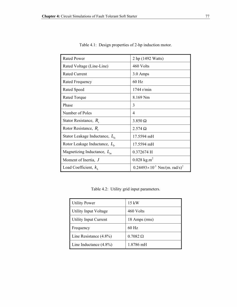
Chapter 4: Circuit Simulations of Fault Tolerant Soft Starter
77
Table 4.1: Design properties of 2-hp induction motor.
Rated Power 2 hp (1492 Watts)
Rated Voltage (Line-Line) 460 Volts
Rated Current 3.0 Amps
Rated Frequency 60 Hz
Rated Speed 1744 r/min
Rated Torque 8.169 Nm
Phase 3
Number of Poles 4
Stator Resistance, sR 3.850 Ω
Rotor Resistance, rR 2.574 Ω
Stator Leakage Inductance, lsL 17.5594 mH
Rotor Leakage Inductance, lrL 17.5594 mH
Magnetizing Inductance, mL 0.372674 H
Moment of Inertia, J 0.028 kg.m2
Load Coefficient, Lk -3 20.24493 10 Nm/(m. rad/s)×
Table 4.2: Utility grid input parameters.
Utility Power 15 kW
Utility Input Voltage 460 Volts
Utility Input Current 18 Amps (rms)
Frequency 60 Hz
Line Resistance (4.8%) 0.7082 Ω
Line Inductance (4.8%) 1.8786 mH

Chapter 4: Circuit Simulations of Fault Tolerant Soft Starter
78
Vram
p*
Vram
p* I_av
g*
Irms_
a
Irms_
b
alph
a_V_
a
alph
a_V_
b
alph
a_i_
a
alph
a_i_
b
11
-C-
alph
a0_b
-C-
alph
a0_a
[ZC_
B2]
Zero
Cros
sing
Volta
geRa
mp
Refe
renc
e(V
ram
p*)
alph
a_de
g
A2
puls
es
alph
a_de
g
B1pu
lses
alph
a_de
g
A1
puls
es
sign
alrm
s
sign
alrm
s
sign
alrm
s
sign
alrm
s
sign
alrm
s
alph
a_de
g
B2pu
lses
Puls
eGe
nera
tor
kp_V
kp_I
kp_I
kp_V
Prop
ortio
nal
Gain
[Imc]
Mea
sure
dTh
ree-
Phas
eM
otor
Curr
ents
[ZC_
B1]
[ZC_
A2]
[ZC_
A1]
[Vm
b]
Mea
sure
dTe
rmin
alVo
ltage
Phas
e-b
[Vm
a]
Mea
sure
dTe
rmin
alVo
ltage
Phas
e-a
Lim
iter
1 s1 s 1 s1 s
ki_V ki_I
ki_I
ki_V In
tegr
alGa
in
[C2]
[C1]
[B2]
[B1]
[A2]
[A1]
1/3
[Ima]
[Imb]
Figure 4.2: Block diagram of soft starter controller in Matlab-Simulink [91].

Chapter 4: Circuit Simulations of Fault Tolerant Soft Starter
79
voltage PI controllers, and 0.3pk = and 32.3ik = for the current PI controllers. The initial
firing/delay angles are set at 110 . The resulting firing/delay angles are fed into a set of pulse
generators for synthesizing a train of gate pulses (high = 1, low = 0) for triggering the SCRs. In
order to simulate the two-phase controls, an active high signal is fed into the gate of both the
SCRs of phase-c so that the switches are turned-on at all time, see Figure 4.2. Finally, the
simulation is carried out at a time step of 10 secµ (or a sampling frequency of 100 kHz).
4.3 Verifications between Closed-Form Analytical and Simulation Results
For convenience of the readers, the closed-form analytical results presented in Chapter 2 of
this dissertation are repeated here for verification purposes with the simulation results. It is
important to note that the simulation results presented here are obtained at nearly the same
operating conditions that were utilized to compute the closed-form analytical results. In addition,
open-loop symmetrical-triggering control was employed here in the simulation.
4.3.1 Healthy Condition
The three-phase line-to-neutral motor voltage waveforms obtained from closed-form
solutions, along with the corresponding simulation waveforms under healthy condition at
60φ = and 90α = are depicted in Figure 4.3(a) and Figure 4.3(b), respectively. As one may
observe, the calculated waveforms are in good agreement with the simulation waveforms. It is
important to mention that the waveforms of Figure 4.3(a) are only valid for transient analysis,
which is the subject of this work, due to the fact that the induced EMF in the windings cannot be
neglected during the steady state operation.
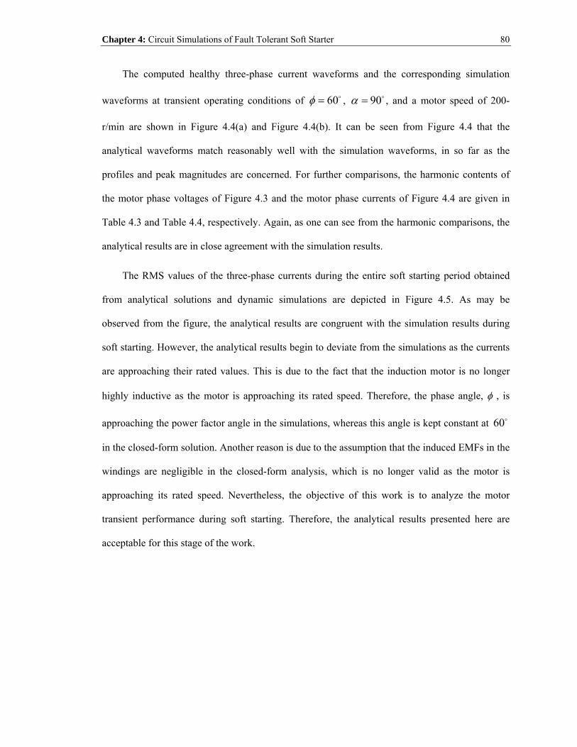
Chapter 4: Circuit Simulations of Fault Tolerant Soft Starter
80
The computed healthy three-phase current waveforms and the corresponding simulation
waveforms at transient operating conditions of 60φ = , 90α = , and a motor speed of 200-
r/min are shown in Figure 4.4(a) and Figure 4.4(b). It can be seen from Figure 4.4 that the
analytical waveforms match reasonably well with the simulation waveforms, in so far as the
profiles and peak magnitudes are concerned. For further comparisons, the harmonic contents of
the motor phase voltages of Figure 4.3 and the motor phase currents of Figure 4.4 are given in
Table 4.3 and Table 4.4, respectively. Again, as one can see from the harmonic comparisons, the
analytical results are in close agreement with the simulation results.
The RMS values of the three-phase currents during the entire soft starting period obtained
from analytical solutions and dynamic simulations are depicted in Figure 4.5. As may be
observed from the figure, the analytical results are congruent with the simulation results during
soft starting. However, the analytical results begin to deviate from the simulations as the currents
are approaching their rated values. This is due to the fact that the induction motor is no longer
highly inductive as the motor is approaching its rated speed. Therefore, the phase angle, φ , is
approaching the power factor angle in the simulations, whereas this angle is kept constant at 60
in the closed-form solution. Another reason is due to the assumption that the induced EMFs in the
windings are negligible in the closed-form analysis, which is no longer valid as the motor is
approaching its rated speed. Nevertheless, the objective of this work is to analyze the motor
transient performance during soft starting. Therefore, the analytical results presented here are
acceptable for this stage of the work.

Chapter 4: Circuit Simulations of Fault Tolerant Soft Starter
81
Analytical
-500
0
500
-500
0
500
Mot
or P
hase
Vol
tage
s (V
)
0 0.01 0.02 0.03 0.04-500
0
500
Time (sec)
Phase-a
Phase-b
Phase-c
(a)
Simulation
-500
0
500
-500
0
500
Mot
or P
hase
Vol
tage
(V)
0 0.01 0.02 0.03 0.04-500
0
500
Time (sec)
Phase-a
Phase-b
Phase-c
(b)
Figure 4.3: Healthy three-phase line-to-neutral motor voltage waveforms at operating conditions of 60φ = and 90α = . (a) Analytical. (b) Simulation.

Chapter 4: Circuit Simulations of Fault Tolerant Soft Starter
82
Analytical
0.3 0.31 0.32 0.33 0.34 0.35-20
-15
-10
-5
0
5
10
15
20
Mot
or C
urre
nts (
A)
Time (sec)
IaIbIc
(a)
Simulation
0.3 0.31 0.32 0.33 0.34 0.35-20
-15
-10
-5
0
5
10
15
20
Mot
or C
urre
nts (
A)
Time (sec)
IaIbIc
(b)
Figure 4.4: Healthy three-phase current waveforms at transient conditions of 60φ = , 90α = , and motor speed of 200-r/min. (a) Analytical. (b) Simulation.

Chapter 4: Circuit Simulations of Fault Tolerant Soft Starter
83
Table 4.3: Harmonic contents of healthy three-phase motor phase voltages – Analytical and Simulation.
Analytical Simulation Harmonic
Order Vma (Volt)
Vmb (Volt)
Vmc (Volt)
Vma (Volt)
Vmb (Volt)
Vmc (Volt)
1 207.30 208.90 208.10 206.22 207.75 207.20 3 0 0 0 0 0 0 5 131.40 131.80 131.90 134.97 134.23 133.66 7 94.11 93.54 94.62 97.38 97.95 98.68 9 0 0 0 0 0 0
11 17.28 18.60 16.41 21.37 21.68 21.40 13 12.45 11.17 13.18 9.49 8.14 9.57 15 0 0 0 0 0 0 17 35.18 35.55 35.23 37.33 36.55 36.01 19 31.37 30.98 31.69 34.11 34.62 35.37 21 0 0 0 0 0 0
Table 4.4: Harmonic contents of healthy three-phase motor currents – Analytical and Simulation.
Analytical Simulation Harmonic
Order Ima (Amps)
Imb (Amps)
Imc (Amps)
Ima (Amps)
Imb (Amps)
Imc (Amps)
1 14.255 14.340 14.326 14.212 14.180 14.234 3 0 0 0 0 0 0 5 2.021 2.027 2.028 2.077 2.035 2.032 7 1.036 1.030 1.042 1.073 1.085 1.109 9 0 0 0 0 0 0
11 0.121 0.131 0.115 0.151 0.159 0.157 13 0.074 0.066 0.078 0.056 0.054 0.059 15 0 0 0 0 0 0 17 0.160 0.162 0.160 0.169 0.161 0.154 19 0.128 0.126 0.129 0.139 0.137 0.149 21 0 0 0 0 0 0

Chapter 4: Circuit Simulations of Fault Tolerant Soft Starter
84
40 50 60 70 80 90 100 1100
5
10
15
SimulationAnalytical
40 50 60 70 80 90 100 1100
5
10
15R
MS
Cur
rent
s (A
)
SimulationAnalytical
40 50 60 70 80 90 100 1100
5
10
15
Alpha Firing Angle (degree)
SimulationAnalytical
Figure 4.5: RMS values of healthy three-phase stator currents from analytical solution and dynamic simulation.
4.3.2 Short-Circuit SCR Switch Fault Condition
The analytical waveforms of the three-phase line-to-neutral motor voltages, and the
corresponding simulation waveforms are illustrated in Figure 4.6(a) and Figure 4.6(b),
respectively. From the figures, one can state that the analytical waveforms are in good agreement
with the simulation waveforms, in so far as the profiles are concerned. Meanwhile, the computed
currents and its associated simulated three-phase motor currents at transient operating conditions
of 60φ = , 90α = , and a motor speed of 400-r/min are shown in Figure 4.7(a) and Figure
4.7(b), respectively. As one can observe, there is a certain degree of similarity between the
analytical and simulation waveforms. Furthermore, the harmonic breakdown of the motor phase
voltages of Figure 4.6 and the motor phase currents of Figure 4.7 are given in Table 4.5 and Table
4.6, respectively. As one can observe from the harmonic comparisons, the analytical results
match fairly well with the simulation results, except for some of the higher-order harmonic

Chapter 4: Circuit Simulations of Fault Tolerant Soft Starter
85
components for which the analytical results tend to over-estimate or under-estimate the higher
harmonic amplitudes. This may be due to the simplifying assumptions built into the analytical
model derivations. The RMS values of the three-phase currents during the entire soft starting
period obtained from analytical solutions and dynamic simulations are depicted in Figure 4.8.
Notice that the currents are unbalanced during starting which can be further validated by the
simulated three-phase currents under a short-circuit SCR switch fault, as illustrated in Figure 4.8.
These unbalanced currents will accordingly lead to undesired transient torque pulsations, as will
be demonstrated next.
Evidently, from the aforementioned results, the simulation work has confirmed the key
analytical results of this investigation. Such efforts validate the fidelity of the closed-form
analytical approach, which provides an alternative means of acquiring the transient motor
performance in lieu of pursuing the simulation approach.
4.4 Motor Performance under Fault Tolerant Operations
In this section, the motor performance resulting from using the resilient closed-loop two-
phase control technique is compared with that when using the conventional symmetrical-
triggering open-loop three-phase as well as two-phase controls. The main thrust is to demonstrate
the efficacy of the present approach under switch fault conditions over the open-loop control
approach, with minimum starting torque transient.
The conventional three-phase soft starter using open-loop voltage control was first
simulated. The results of the three-phase motor currents are shown in Figure 4.9(a). As one may
observe therein, the motor currents have smooth starting profiles as the firing angle is decreasing,
with low starting currents. To demonstrate the voltage unbalance effects due to open-loop two-
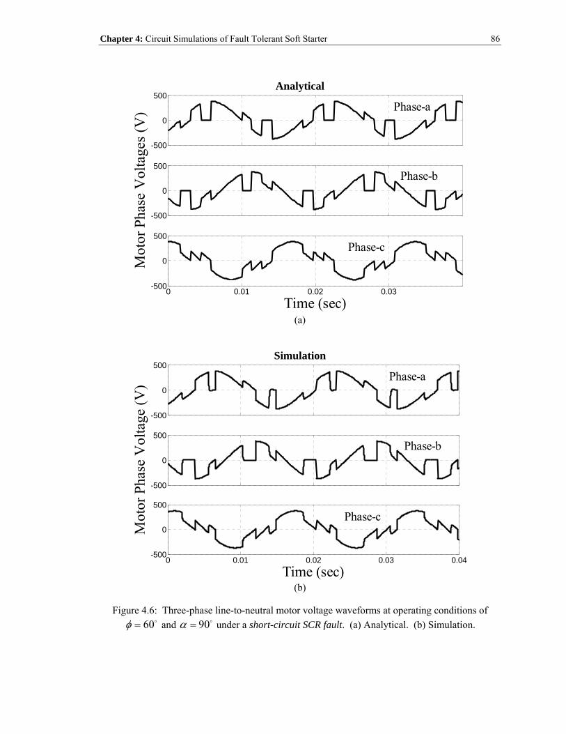
Chapter 4: Circuit Simulations of Fault Tolerant Soft Starter
86
Analytical
-500
0
500
-500
0
500
Mot
or P
hase
Vol
tage
s (V
)
0 0.01 0.02 0.03-500
0
500
Time (sec)
Phase-a
Phase-b
Phase-c
(a)
Simulation
-500
0
500
-500
0
500
Mot
or P
hase
Vol
tage
(V)
0 0.01 0.02 0.03 0.04-500
0
500
Time (sec)
Phase-a
Phase-b
Phase-c
(b)
Figure 4.6: Three-phase line-to-neutral motor voltage waveforms at operating conditions of 60φ = and 90α = under a short-circuit SCR fault. (a) Analytical. (b) Simulation.
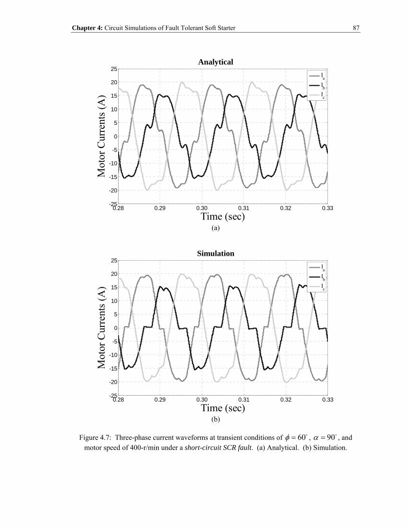
Chapter 4: Circuit Simulations of Fault Tolerant Soft Starter
87
Analytical
0.28 0.29 0.30 0.31 0.32 0.33-25
-20
-15
-10
-5
0
5
10
15
20
25
Mot
or C
urre
nts (
A)
Time (sec)
IaIbIc
(a)
Simulation
0.28 0.29 0.30 0.31 0.32 0.33-25
-20
-15
-10
-5
0
5
10
15
20
25
Mot
or C
urre
nts (
A)
Time (sec)
IaIbIc
(b)
Figure 4.7: Three-phase current waveforms at transient conditions of 60φ = , 90α = , and motor speed of 400-r/min under a short-circuit SCR fault. (a) Analytical. (b) Simulation.

Chapter 4: Circuit Simulations of Fault Tolerant Soft Starter
88
Table 4.5: Harmonic contents of three-phase motor phase voltages under a short-circuit SCR fault – Analytical and Simulation.
Analytical Simulation Harmonic
Order Vma (Volt)
Vmb (Volt)
Vmc (Volt)
Vma (Volt)
Vmb (Volt)
Vmc (Volt)
1 259.30 220.80 318.80 270.97 200.22 300.35 3 54.98 52.48 107.50 48.46 41.81 102.99 5 116.60 116.20 43.55 117.73 124.22 39.75 7 82.65 82.85 32.03 75.70 72.70 36.03 9 17.12 19.23 36.30 49.33 20.35 29.35
11 15.62 16.70 5.64 35.88 27.28 28.45 13 10.67 9.60 4.31 41.29 44.65 6.55 15 10.88 8.60 19.44 4.82 15.20 17.05 17 31.60 31.24 11.32 3.73 4.96 2.30 19 27.35 27.55 11.01 9.32 13.15 7.18 21 6.11 7.98 14.03 9.48 15.35 14.73
Table 4.6: Harmonic contents of three-phase motor currents under a short-circuit SCR fault – Analytical and Simulation.
Analytical Simulation Harmonic
Order Ima (Amps)
Imb (Amps)
Imc (Amps)
Ima (Amps)
Imb (Amps)
Imc (Amps)
1 18.752 14.043 21.666 19.621 13.413 20.740 3 1.397 1.333 2.731 1.350 1.300 2.605 5 1.793 1.787 0.670 1.807 1.892 0.628 7 0.910 0.912 0.353 0.806 0.760 0.381 9 0.147 0.165 0.312 0.417 0.157 0.261
11 0.110 0.117 0.040 0.253 0.205 0.206 13 0.063 0.057 0.026 0.247 0.269 0.034 15 0.056 0.044 0.100 0.027 0.068 0.082 17 0.144 0.142 0.051 0.017 0.019 0.005 19 0.111 0.112 0.045 0.035 0.045 0.026 21 0.022 0.029 0.052 0.037 0.062 0.055

Chapter 4: Circuit Simulations of Fault Tolerant Soft Starter
89
40 50 60 70 80 90 100 1100
10
20
SimulationAnalytical
40 50 60 70 80 90 100 1100
10
20R
MS
Cur
rent
s (A
)
SimulationAnalytical
40 50 60 70 80 90 100 1100
10
20
Alpha Firing Angle (degree)
SimulationAnalytical
Figure 4.8: RMS values of three-phase stator currents from analytical solution and dynamic simulation under a short-circuit SCR fault.
phase operation, the control method applied to the three-phase soft starter was utilized except that
one phase of the back-to-back thyristors is always maintained in the “on” state. In reality, this is
equivalent to isolating the faulty switch by closing the corresponding by-pass contactor so that
there is a direct electrical connection between the ac mains and the associated motor phase. The
results of the motor phase currents are depicted in Figure 4.9(b). Notice the high motor current
unbalances during the starting transients. This is not the case for the present closed-loop two-
phase control, the results of which are illustrated in Figure 4.9(c). As may be noted in Figure
4.9(c), the three-phase motor currents have reasonably smooth starting profiles, which indicate
significant starting transient improvement, in comparisons to that of Figure 4.9(b) due to open-
loop two-phase control. Even though the currents of Figure 4.9(c) have a higher breakdown
current value than that of Figure 4.9(b), the starting inrush currents are lower as compared to that
of Figure 4.9(b).

Chapter 4: Circuit Simulations of Fault Tolerant Soft Starter
90
To further demonstrate the fineness of the present approach, the current space-vector plots of
the motor currents in the form of 2 3 4 32 3 ( )j js q d a b ci i ji i i e i eπ π= + = ⋅ + + are given in Figure
4.10(a), (b), and (c), for the three-phase open-loop, the two-phase open-loop, and the proposed
two-phase closed-loop controls, respectively. The current space-vector plot due to three-phase
open-loop control, see Figure 4.10(a), exhibits a circular locus with the 12 distinct switching
states. On the other hand, the two-phase open-loop control results in an elliptic locus with higher
starting currents, as shown in Figure 4.10(b). Notice the 8 distinct switching states that the locus
presents due to this control method. An improved starting transient of the current space-vector
plot with a circular locus can be observed from Figure 4.10(c) for the proposed closed-loop two-
phase control approach.
The developed motor torque profiles for all three control cases are depicted in Figure 4.11.
Again, one can see a smooth starting profile with minimum torque pulsations in Figure 4.11(a).
However, this is not the case under open-loop two-phase control, as can be observed from Figure
4.11(b). An improved starting torque profile for the proposed approach is illustrated in Figure
4.11(c). It can be seen from the figure that the starting torque pulsations are significantly reduced
as compared to those of Figure 4.11(b).
4.5 Summary
The first part of this chapter is to verify the accuracy of the closed-form analytical results
versus the simulation results. It has been shown that the analytical results are in good
correspondence with the simulation results, which raises confidence in the fidelity and value of
the analytical approach. Such efforts provide an alternative means of analyzing the transient
performance of the motor besides using the simulation approach. The second part of the work
involves comparing the motor performance under three different control cases, namely, three-

Chapter 4: Circuit Simulations of Fault Tolerant Soft Starter
91
phase open-loop, two-phase open-loop, and proposed two-phase closed-loop controls. The
present fault tolerant resilient control has demonstrated reduced starting inrush currents, and
consequently reduced starting torque pulsations under thyristor fault in one phase of the soft
starter, as compared to the two-phase open-loop control case. These promising results
demonstrate the feasibility of the proposed strategy for improving the reliability of an industrial-
type three-phase soft starter system at a modest cost increase.

Chapter 4: Circuit Simulations of Fault Tolerant Soft Starter
92
0 0.1 0.2 0.3 0.4 0.5 0.6 0.7 0.8-30
-20
-10
0
10
20
30
Mot
or C
urre
nts (
A)
Time (sec)
IaIbIc
(a)
0 0.1 0.2 0.3 0.4 0.5 0.6 0.7 0.8-30
-20
-10
0
10
20
30
Mot
or C
urre
nts (
A)
Time (sec)
IaIbIc
(b)
0 0.1 0.2 0.3 0.4 0.5 0.6 0.7 0.8-30
-20
-10
0
10
20
30
Mot
or C
urre
nts (
A)
Time (sec)
IaIbIc
(c)
Figure 4.9: Simulation results of three-phase current waveforms. (a) 3-phase open-loop control. (b) 2-phase open-loop control. (c) Proposed 2-phase closed-loop control.

Chapter 4: Circuit Simulations of Fault Tolerant Soft Starter
93
-30 -20 -10 0 10 20 30-30
-20
-10
0
10
20
30
I d (A)
Iq (A)
(a)
-30 -20 -10 0 10 20 30-30
-20
-10
0
10
20
30
I d (A)
Iq (A)
(b)
-30 -20 -10 0 10 20 30-30
-20
-10
0
10
20
30
I d (A)
Iq (A)
(c)
Figure 4.10: Simulation results of current space-vector plots. (a) 3-phase open-loop control. (b) 2-phase open-loop control. (c) Proposed 2-phase closed-loop control.
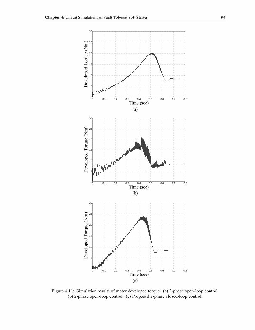
Chapter 4: Circuit Simulations of Fault Tolerant Soft Starter
94
0 0.1 0.2 0.3 0.4 0.5 0.6 0.7 0.80
5
10
15
20
25
30
Dev
elop
ed T
orqu
e (N
m)
Time (sec) (a)
0 0.1 0.2 0.3 0.4 0.5 0.6 0.7 0.80
5
10
15
20
25
30
Dev
elop
ed T
orqu
e (N
m)
Time (sec) (b)
0 0.1 0.2 0.3 0.4 0.5 0.6 0.7 0.80
5
10
15
20
25
30
Dev
elop
ed T
orqu
e (N
m)
Time (sec) (c)
Figure 4.11: Simulation results of motor developed torque. (a) 3-phase open-loop control. (b) 2-phase open-loop control. (c) Proposed 2-phase closed-loop control.

95
CHAPTER 5
5 HARDWARE EXPERIMENTS OF FAULT
TOLERANT SOFT STARTER
5.1 Introduction
With the analytical and simulation portions of the present fault tolerant soft starter, including
the theoretical design of the soft starter controller, accomplished and documented in the foregoing
chapters, one is now at a stage of presenting the hardware experimental results. The test operating
conditions, as well as the controller design parameters, were set as close as possible to their
values given earlier in association with the simulation conditions. This was done for comparison
purposes between the simulation results given in Chapter 4 and the test results which will be
given here. For these purposes, some of the analytical and simulation results presented earlier are
repeated here for the convenience of the reader. The target test motor chosen for the experimental
testing is the 2-hp, 4-pole, three-phase induction motor, whose machine parameters were given
earlier in Chapter 4 and were used in the simulation work. Evidently from the experimental
results as will be shown later on, the fault tolerant control scheme alleviates the starting torque
pulsations under SCR switch fault condition. Accordingly, such promising results demonstrate

Chapter 5: Hardware Experiments of Fault Tolerant Soft Starter 96
the feasibility and validity of the present approach. In the following, the hardware prototype is
first described, followed by the test results.
5.2 Hardware Prototype
The configuration of the experimental setup is shown schematically in Figure 5.1. The setup
consists of a 460-Volt utility grid supply feeding a three-phase SCR bridge, which acts as a soft
starter to supply controlled voltages to a three-phase induction motor during soft starting. The
power rating of the SCR bridge is chosen such that the direct-online-starting current of the target
motor is within the limit of the current rating of the chosen SCRs. Typically, the maximum
current amplitude (rms) during line-starting of a motor is about 6 to 8 times of the motor rated
current value [22]. On the other hand, for the case of soft starting, typically the maximum current
amplitude (rms) is measured to be about 3 to 5 times that of the motor rated current value [22].
The SCR bridge was mounted on a oversized heat sink, originally intended for a 15-hp drive, see
Figure 5.2(a). With this oversized heat sink, along with the use of a fan as the cooling
mechanism, the thermal issues of the power structure were not of major concern. Sunbber circuits
in the form of RC elements were also incorporated to reduce any switching transients caused by
the process of commutation of the SCRs. Meanwhile, a DSP-based control board from Texas
Instruments (Model: TMS320F2812) were utilized to control the switching sequences of the SCR
switches [92]. Voltage and current feedbacks through the use of analog signal conditioning
circuits and current transducers (from LEM) are fed into the analog inputs of the DSP board, and
the firing pulses in the form of digital signals were accordingly generated. The gate drive
interface between the high power stages of the switches and the low power stages of the DSP was
realized by means of a set of pulse transformers. The main purpose of such type of interface is to
provide electrical galvanic isolations between the high and low power stages, as well as to
provide sufficient currents to the gates of the SCRs for turning-on. The EMI/EMC noise of the

Chapter 5: Hardware Experiments of Fault Tolerant Soft Starter 97
present hardware prototype was minimized through the use of decoupling capacitors in various
parts of the signal conditioning circuits. Digital software-based low-pass filters, of the 5th order
Butterworth type [93], were also implemented in the DSP to suppress any EMI noise that might
be imposed on the measured signals. The data measurement was carried out using a data
acquisition (DAQ) system from National Instruments (Model: PCI-6052E) at a data measurement
sampling rate of 50 kSamples/sec [94]. This system allows measurements of up to 8 analog
signals, which are virtually impossible to achieve from an ordinary oscilloscope. Again, the
hardware prototype of the present configuration is depicted in Figure 5.2(a). Detailed designs and
specifications of the present hardware prototype, including circuit design and component
selections, are described in Appendix A of this dissertation.
As mentioned earlier, the test motor is a 2-hp, 4-pole, three-phase induction motor, with a
full-load rating of 8.169 Nm at a rated speed of 1744 r/min. This is the same motor that had been
used during the simulation process of this work. The motor is coupled to a dynamometer from
Magtrol Corporation through a love joy coupler, as shown in Figure 5.2(b). This Magtrol
dynamometer, which functions as a mechanical load, is capable of supplying up to 12 Nm. It is
important to mention that the load torque supplied by this dynamometer is a constant type, which
is different from the fan type of load used in the earlier simulation work in Chapter 4. The
specifications of the hardware prototype are listed in Figure 5.1, as well as in Table 5.1. For
further details, Appendix A should be consulted.
As was indicated in Chapter 3 of this dissertation, the present control scheme requires the
use of PI controllers for closed-loop feedback control purposes. The DSP-based controller
proportional gains for both the voltage and current feedback loops were selected to be the same as
those obtained from the theoretical analysis carried out in Chapter 3 and those used in the circuit
simulations. That is, 0.0013pk = for the voltage loop, and 0.3pk = for the current loop.
However, the DSP-based controller integral gains which were obtained from the theoretical

Chapter 5: Hardware Experiments of Fault Tolerant Soft Starter 98
a
b
cn
Indu
ctio
nM
otor
i a i b i c
Vsa
Vsb Vsc
AC
Mot
orU
tility
Rsa
Rsb Rsc
L sa L sb L sc
0.70
81.
88m
H
0.70
81.
88m
H
0.70
81.
88m
H
Con
tact
or
Vol
tage
Sen
sor
(Sou
rce)
Vsa
GN
D
Vsb
Vs c
R1
R2
R3
SK
45
UT
16S
CR
Brid
ge
C1
C2
C3
5711
2pF
5711
2pF
5711
2pF
SC
R1
SC
R2
SC
R3
Vol
tage
Sen
sor
(Mot
or)
Vma
Vmb
Vm
c
Cur
rent
Sens
or(M
otor
)
Ima
Imb
Imc
15 k
W46
0 Va
c18
Am
ps60
Hz
4.8
%Z
Spec
ifica
tions
1. U
tility
: 15
kW, 4
60 V
ac, 1
8 Am
ps, 6
0 H
z, 4
.8 %
Z2.
Con
tact
or: 3
-Pha
se, 1
20 V
ac c
oil,
90 A
mps
/ 60
0 V
ac M
ax R
atin
gs3.
SC
R B
ridge
: Sem
ikro
n, S
emito
p 3,
SK
45 U
T 16
, 3-P
hase
, 47
Amps
/ 16
00 V
4. S
nubb
er: R
= 5
7 oh
ms
(5%
), C
= 1
12 p
F (2
0%) (
Mod
el: X
5F, 3
kV
ratin
g)5.
Fan
: 24
Vdc
, 0.2
8 A
mps
, 6.7
Wat
ts, R
ed+
Bla
ck-
6. M
otor
: 2 H
P, 4
-Pol
e, 2
30/4
60 V
ac, 6
.0/3
.0 A
mps
, 174
4 rp
m, 6
0 H
z7.
DSP
Con
trol
ler:
Texa
s In
stru
men
ts, T
MS
320F
2812
, Fix
ed-P
oint
DS
P8.
Sen
sor:
LEM
, Cur
rent
Tra
nsdu
cer L
F 30
5-S,
300
Am
ps (r
ms)
9. S
igna
l Con
ditio
ning
: Pul
se T
rans
form
ers
+ A
nalo
g C
ircui
ts10
. Dat
a A
cqui
sitio
n: N
atio
nal I
nstru
men
ts, P
CI-6
052E
, 333
kSa
mpl
es/s
ec
Gat
ePu
lses
Sign
alC
ondi
tioni
ngC
ircui
ts
DSP
Con
trol
ler
Volta
ge &
Cur
rent
Feed
back
s
DA
QSy
stem
Figure 5.1: Schematic of experimental setup of induction motor-soft starter system.

Chapter 5: Hardware Experiments of Fault Tolerant Soft Starter 99
SCR Bridges
Current Sensors
Pulse Transformers +
Signal Conditioning Boards
TI DSP Board
Snubber
(a)
2-hp Induction Motor
Dyne
Dyne Controller
(b)
Figure 5.2: Test rigs. (a) Soft starter. (b) Induction motor and dynamometer.

Chapter 5: Hardware Experiments of Fault Tolerant Soft Starter 100
Table 5.1: Specifications of hardware prototype.
Utility Utility Input Voltage (Line-To-Line) 460 Volts Frequency 60 Hz Line Resistance (4.8%) 0.7082 Ω Line Inductance (4.8%) 1.8786 mH
SCR Bridge Current / Voltage Ratings (Max) 47 Amps / 1600 Volts (rms) Snubber Circuits R = 57 Ω, C = 112 pF
Induction Motor Rated Power 2 hp (1492 Watts) Rated Voltage (Line-To-Line) 460 Volts Rated Current 3.0 Amps Rated Frequency 60 Hz Rated Speed 1744 r/min Rated Torque 8.169 Nm Phase 3 Number of Poles 4
Dynamometer (Magtrol) Mechanical Load (Constant Type) Up to 12 Nm
DSP Board (TI TMS320F2812) Execution Cycle 10 kHz Digital Low-pass Filter 5th order Butterworth type PI Gains for Voltage Loop 0.0013pk = , 0.5ik = PI Gains for Current Loop 0.3pk = , 1.5ik = Anti-windup Gains for Both Loops 0.2ck =
DAQ System (NI PCI-6052E) System Sampling Rate 333 kSamples/sec Acutal Measurement Rate 50 kSamples/sec Number of Analog Input Channels 8
Current Transducer Current Rating (Max) 300 Amps (rms)

Chapter 5: Hardware Experiments of Fault Tolerant Soft Starter 101
analysis, that is, 7.27ik = for the voltage loop and 32.3ik = for the current loop, have been
first reduced by a factor of 10. The reason for doing so is due to the fact that the circuit simulation
was carried out at a sampling frequency of 100 kHz, while the interrupt service routine in the
DSP main program is executing at 10 kHz. Hence, the designed integral gains need to be reduced
by one order of magnitude [90]. Further fine tuning, for the purposes of stabilizing the control
loop, as well as reducing noise susceptibility, results in the following integral gains: 0.5ik = for
the voltage loop and 1.5ik = for the current loop. In addition, an anti-windup scheme was also
incorporated into the PI controller design. This is to avoid instability in the PI controller due to
saturation in the integral loop, especially during start up when the error between the reference
input and the control output is large [90]. The anti-windup gains for both the voltage and current
loops were accordingly chosen to be 0.2ck = .
5.3 Experimental Results
5.3.1 Comparisons with Simulation and Analytical Results
In Chapter 4 of this dissertation, the simulation results were compared with the analytical
results obtained from Chapter 3 under both healthy and faulty conditions. The resulting
comparisons indicated a good degree of similarity/agreement between the analytical and
simulation results. In this chapter, those results are repeated here for comparison with the
experimental test results for further verification purposes. This is in order to validate and
demonstrate the accuracy/fidelity of the analytical work being done thus far.
The test results of the healthy three-phase motor line-to-neutral voltages during soft starting
under full-load condition are depicted in Figure 5.3(a), along with the corresponding simulation
and analytical results given in Figure 5.3(b) and Figure 5.3(c), respectively. Notice the close

Chapter 5: Hardware Experiments of Fault Tolerant Soft Starter 102
agreement between each individual waveform for phases-a, b, and c. The corresponding healthy
three-phase motor currents under the same condition for the test, simulation, and analytical work
are shown in Figure 5.4(a), (b), and (c), respectively. It can be observed from Figure 5.4 that there
is a reasonable degree of agreement between those waveforms. Furthermore, the harmonic
contents of the motor phase voltages of Figure 5.3 and the motor phase currents of Figure 5.4 are
given in Table 5.2 and Table 5.3, respectively. Again, there is a considerable degree of similarity
between the trends of the harmonic components of the test, simulation, and analytical results,
except for some of the higher-order harmonics, and third harmonic as well as its multiples 9th,
15th, etc. This may be due to the fact that the machine’s magnetic core saturation effects are
neglected in the simulation and analytical work, while such saturation effects are inherently
present in the actual test motor. This is also the reason for the presence of a positive-sequence 3rd
harmonic component and its multiples, as indicated in the test columns of the voltage and current
in both tables.
Meanwhile, the experimental work was repeated in the event of an SCR short-circuit switch
fault, by turning-on the SCRs of phase-c continuously, to emulate the effect of a bypass contactor
that would have been used in practice. The measured results of the three-phase motor phase
voltages are depicted in Figure 5.5(a). The associated simulation and analytical results are given
in Figure 5.5(b) and (c), respectively. Again, therein, one can notice the similarity between those
voltage waveforms in so far as the profiles are concerned. The experimental results also show the
unsymmetrical nature of the voltage waveforms under faulty condition. The corresponding three-
phase motor currents obtained from test, simulation, and analytical work under faulty condition
are illustrated in Figure 5.6(a), (b), and (c), respectively. It can be noticed from the test results in
Figure 5.6(a) that the measured currents exhibit the same unbalanced nature as the simulation and
analytical results, when subjected to a short-circuit switch fault. In addition, the harmonic
breakdown of the motor phase voltages of Figure 5.5 and the motor phase currents of Figure 5.6

Chapter 5: Hardware Experiments of Fault Tolerant Soft Starter 103
are listed in Table 5.4 and Table 5.5, respectively. Again, upon comparison, there is a certain
degree of agreement in trend among these results, except for some of the higher-order harmonic
components due to the effects of the machine’s magnetic saturation being present in the test, and
as mentioned earlier neglected in both the simulation and analytical models. The fact that the
impressed voltages on the motor windings are unbalanced, under faulty condition, is also a
contributing factor to the presence of the positive-sequence 3rd harmonic component and its
multiples in the test, simulation, and analytical results, see Table 5.4 and Table 5.5.
It should be mentioned here that due to the inaccessibility of the motor neutral connection,
the measured motor line-to-neutral voltages presented herein in the test data were indirectly
acquired through the use of the line-to-line voltage measurements, assuming a balanced three-
phase motor, which would lead to line-to-neutral voltages which can be expressed and computed
as follows:
( )
( )
( )
131313
an ab ca
bn bc ab
cn ca bc
v v v
v v v
v v v
= −
= −
= −
(5.1)

Chapter 5: Hardware Experiments of Fault Tolerant Soft Starter 104
Test
Mot
or P
hase
Vol
tage
s (20
0 V
/div
)
Time (10 ms/div)
Phase-a
Phase-b
Phase-c
0
0
0
(a)
Simulation
-500
0
500
-500
0
500
Mot
or P
hase
Vol
tage
(V)
0 0.01 0.02 0.03 0.04-500
0
500
Time (sec)
Phase-a
Phase-b
Phase-c
(b)
Analytical
-500
0
500
-500
0
500
Mot
or P
hase
Vol
tage
s (V
)
0 0.01 0.02 0.03 0.04-500
0
500
Time (sec)
Phase-a
Phase-b
Phase-c
(c)
Figure 5.3: Healthy three-phase line-to-neutral motor voltage waveforms. (a) Test. (b) Simulation. (c) Analytical.

Chapter 5: Hardware Experiments of Fault Tolerant Soft Starter 105
Test
0
Mot
or C
urre
nts (
5 A
/div
)
Time (10 ms/div)
IaIbIc
(a)
Simulation
0.3 0.31 0.32 0.33 0.34 0.35-20
-15
-10
-5
0
5
10
15
20
Mot
or C
urre
nts (
A)
Time (sec)
IaIbIc
(b)
Analytical
0.3 0.31 0.32 0.33 0.34 0.35-20
-15
-10
-5
0
5
10
15
20
Mot
or C
urre
nts (
A)
Time (sec)
IaIbIc
(c)
Figure 5.4: Healthy three-phase current waveforms. (a) Test. (b) Simulation. (c) Analytical.

Chapter 5: Hardware Experiments of Fault Tolerant Soft Starter 106
Table 5.2: Harmonic contents of healthy three-phase motor phase voltages – Test, Simulation, and Analytical.
Test Simulation Analytical Harmonic
Order Vma (Volt)
Vmb (Volt)
Vmc (Volt)
Vma (Volt)
Vmb (Volt)
Vmc (Volt)
Vma (Volt)
Vmb (Volt)
Vmc (Volt)
1 197.91 197.10 199.35 206.22 207.75 207.20 207.30 208.90 208.10 3 8.31 8.51 8.77 0 0 0 0 0 0 5 118.22 123.95 127.16 134.97 134.23 133.66 131.40 131.80 131.90 7 86.95 88.52 86.25 97.38 97.95 98.68 94.11 93.54 94.62 9 5.16 5.89 4.92 0 0 0 0 0 0
11 25.85 25.05 26.82 21.37 21.68 21.40 17.28 18.60 16.41 13 22.95 24.45 23.94 9.49 8.14 9.57 12.45 11.17 13.18 15 4.76 4.51 4.92 0 0 0 0 0 0 17 27.55 24.90 29.90 37.33 36.55 36.01 35.18 35.55 35.23 19 25.60 24.62 22.03 34.11 34.62 35.37 31.37 30.98 31.69 21 3.12 2.86 3.35 0 0 0 0 0 0
Table 5.3: Harmonic contents of healthy three-phase motor currents – Test, Simulation, and Analytical.
Test Simulation Analytical Harmonic
Order Ima (A)
Imb (A)
Imc (A)
Ima (A)
Imb (A)
Imc (A)
Ima (A)
Imb (A)
Imc (A)
1 13.681 13.550 13.793 14.212 14.180 14.234 14.255 14.340 14.326 3 0.208 0.246 0.265 0 0 0 0 0 0 5 2.680 2.781 2.824 2.077 2.035 2.032 2.021 2.027 2.028 7 0.956 0.985 0.889 1.073 1.085 1.109 1.036 1.030 1.042 9 0.112 0.168 0.090 0 0 0 0 0 0
11 0.245 0.309 0.341 0.151 0.159 0.157 0.121 0.131 0.115 13 0.178 0.101 0.193 0.056 0.054 0.059 0.074 0.066 0.078 15 0.089 0.055 0.095 0 0 0 0 0 0 17 0.152 0.118 0.146 0.169 0.161 0.154 0.160 0.162 0.160 19 0.112 0.110 0.092 0.139 0.137 0.149 0.128 0.126 0.129 21 0.056 0.044 0.069 0 0 0 0 0 0

Chapter 5: Hardware Experiments of Fault Tolerant Soft Starter 107
Test
Mot
or P
hase
Vol
tage
s (20
0 V
/div
)
Time (10 ms/div)
0
0
0
Phase-a
Phase-b
Phase-c
(a)
Simulation
-500
0
500
-500
0
500
Mot
or P
hase
Vol
tage
(V)
0 0.01 0.02 0.03 0.04-500
0
500
Time (sec)
Phase-a
Phase-b
Phase-c
(b)
Analytical
-500
0
500
-500
0
500
Mot
or P
hase
Vol
tage
s (V
)
0 0.01 0.02 0.03-500
0
500
Time (sec)
Phase-a
Phase-b
Phase-c
(c)
Figure 5.5: Three-phase line-to-neutral motor voltage waveforms under a short-circuit SCR fault. (a) Test. (b) Simulation. (c) Analytical.

Chapter 5: Hardware Experiments of Fault Tolerant Soft Starter 108
Test
0
Mot
or C
urre
nts (
5 A
/div
)
Time (10 ms/div)
IaIbIc
(a)
Simulation
0.28 0.29 0.30 0.31 0.32 0.33-25
-20
-15
-10
-5
0
5
10
15
20
25
Mot
or C
urre
nts (
A)
Time (sec)
IaIbIc
(b)
Analytical
0.28 0.29 0.30 0.31 0.32 0.33-25
-20
-15
-10
-5
0
5
10
15
20
25
Mot
or C
urre
nts (
A)
Time (sec)
IaIbIc
(c)
Figure 5.6: Three-phase current waveforms under a short-circuit SCR fault. (a) Test. (b) Simulation. (c) Analytical.
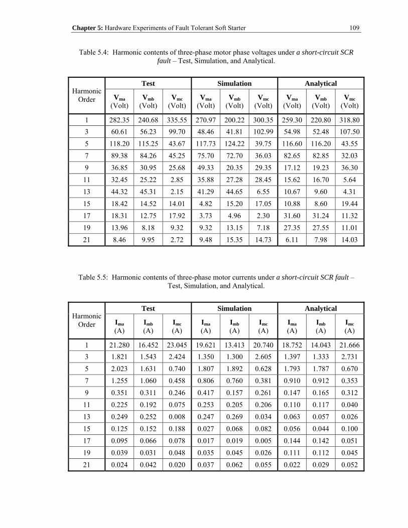
Chapter 5: Hardware Experiments of Fault Tolerant Soft Starter 109
Table 5.4: Harmonic contents of three-phase motor phase voltages under a short-circuit SCR fault – Test, Simulation, and Analytical.
Test Simulation Analytical Harmonic
Order Vma (Volt)
Vmb (Volt)
Vmc (Volt)
Vma (Volt)
Vmb (Volt)
Vmc (Volt)
Vma (Volt)
Vmb (Volt)
Vmc (Volt)
1 282.35 240.68 335.55 270.97 200.22 300.35 259.30 220.80 318.80 3 60.61 56.23 99.70 48.46 41.81 102.99 54.98 52.48 107.50 5 118.20 115.25 43.67 117.73 124.22 39.75 116.60 116.20 43.55 7 89.38 84.26 45.25 75.70 72.70 36.03 82.65 82.85 32.03 9 36.85 30.95 25.68 49.33 20.35 29.35 17.12 19.23 36.30
11 32.45 25.22 2.85 35.88 27.28 28.45 15.62 16.70 5.64 13 44.32 45.31 2.15 41.29 44.65 6.55 10.67 9.60 4.31 15 18.42 14.52 14.01 4.82 15.20 17.05 10.88 8.60 19.44 17 18.31 12.75 17.92 3.73 4.96 2.30 31.60 31.24 11.32 19 13.96 8.18 9.32 9.32 13.15 7.18 27.35 27.55 11.01 21 8.46 9.95 2.72 9.48 15.35 14.73 6.11 7.98 14.03
Table 5.5: Harmonic contents of three-phase motor currents under a short-circuit SCR fault – Test, Simulation, and Analytical.
Test Simulation Analytical Harmonic
Order Ima (A)
Imb (A)
Imc (A)
Ima (A)
Imb (A)
Imc (A)
Ima (A)
Imb (A)
Imc (A)
1 21.280 16.452 23.045 19.621 13.413 20.740 18.752 14.043 21.666 3 1.821 1.543 2.424 1.350 1.300 2.605 1.397 1.333 2.731 5 2.023 1.631 0.740 1.807 1.892 0.628 1.793 1.787 0.670 7 1.255 1.060 0.458 0.806 0.760 0.381 0.910 0.912 0.353 9 0.351 0.311 0.246 0.417 0.157 0.261 0.147 0.165 0.312
11 0.225 0.192 0.075 0.253 0.205 0.206 0.110 0.117 0.040 13 0.249 0.252 0.008 0.247 0.269 0.034 0.063 0.057 0.026 15 0.125 0.152 0.188 0.027 0.068 0.082 0.056 0.044 0.100 17 0.095 0.066 0.078 0.017 0.019 0.005 0.144 0.142 0.051 19 0.039 0.031 0.048 0.035 0.045 0.026 0.111 0.112 0.045 21 0.024 0.042 0.020 0.037 0.062 0.055 0.022 0.029 0.052

Chapter 5: Hardware Experiments of Fault Tolerant Soft Starter 110
5.3.2 Motor Performance under Fault Tolerant Operations
In this section, the experimental results of motor performance resulting from using the
resilient closed-loop two-phase control technique are compared with those when using the
conventional symmetrical-triggering open-loop three-phase control approach as well as two-
phase control approach. The open-loop three-phase control approach and two-phase control
approach were carried out under the conditions of an initial locked-rotor torque percentage of
40%, and a soft start ramp time of 5 seconds. On the other hand, for the case of the proposed
closed-loop two-phase control technique, the test conditions were set at an initial voltage of 200-
Volt, a final voltage of 265-Volt, and a soft start ramp time of 5 seconds. The PI controller gains
were those given in Table 5.1. The initial firing delay angles for all cases were set at 110 .
Finally, all the testing was carried out under full-load motor condition.
Due to limited laboratory facilities, the present dynamometer setup of Figure 5.2(b) is not
equipped with a torque transducer. Therefore, an implicit method of obtaining the motor airgap or
developed torque was utilized here which can be expressed in terms of the measured motor
quantities, as follows [95]:
( ) ( )
( ) ( ) 2 3
airgap dev a b ca s c a
c a ab s a b
PT T i i v R i i dt
i i v R i i dt
= = − − −⎡ ⎤⎣ ⎦
− − − −⎡ ⎤⎣ ⎦
∫
∫ (5.2)
where, P is the number of poles, and sR is the stator equivalent series resistance per phase. As
one can see from (5.2), the motor airgap or developed torque can be implicitly computed using
the measured motor quantities, which can be easily accessible from the present DAQ system.
First, the test results obtained under direct-line-starting are given in Figure 5.7(a) and (b) for
the motor phase currents and airgap (developed) torque, respectively, under normal/healthy motor
condition. As expected, the starting transients are characterized by high inrush currents and high

Chapter 5: Hardware Experiments of Fault Tolerant Soft Starter 111
torque pulsations. Next, the test waveforms of the three-phase motor currents under conventional
soft-starter 3-phase open-loop control, along with the corresponding simulation waveforms are
depicted in Figure 5.8(a) and (b), respectively. As one can observe from both figures, the test and
simulation waveforms are in good agreement with one another in so far as the starting profiles are
concerned. The currents from both figures, test and simulations, have a starting value of around
10 Amps and a peak value of around 20 Amps. The corresponding motor airgap (developed)
torque profiles computed from the experiment and simulation current and voltage data are shown
in Figure 5.9(a) and (b), respectively. One can notice that the test waveform of the torque profile,
see Figure 5.9(a), consists of more ripple contents than that of the simulation of Figure 5.9(b),
which can be attributed to a number of possible factors. The first factor can be due to the fact that
the machine’s magnetic core saturation was neglected in the simulation process owing to the use
of the dq reference frame representation of the induction motor, in which this assumption of
linearity is inherent. In reality, during starting, a motor is subjected to considerable magnetic
saturation effects owing to the high starting transient currents, which leads to the presence of
space/time harmonics imposed on the currents, and consequently the torque. The second factor
may be due to drift problems in the integrator terms of the torque expression of (5.2), which can
be attributed to the presence of small dc offsets in the measurements of the voltages and currents.
These dc offsets or errors, which can be caused by either the sensor itself or the data acquisition
system, will accumulate during the integration process associated with obtaining the torque
indirectly through the use of (5.2). As a result, these cumulative errors introduce noises in the
computation process. Nevertheless, both the measured and simulated motor torques have similar
starting profiles. One should also notice that the average starting torque values from both the test
and simulation are around 2 Nm, and their maximum values are both around 20 Nm, see Figure
5.9. Meanwhile, one can notice a discrepancy in the time scales of both the test (400 ms/div) and
simulation (100 ms/div) waveforms of Figure 5.8 and Figure 5.9. This is mainly due to the
different types of load used in the experimental and simulation work. Since a constant load torque

Chapter 5: Hardware Experiments of Fault Tolerant Soft Starter 112
(~ 8 Nm) was utilized in the experimental test, it is anticipated that the motor will take longer to
accelerate and reach its steady-state condition, as compared to the simulation results in which a
fan load was used to provide a mechanical load torque of 8.169 Nm at the rated speed.
The experiment was repeated under the same operating condition, except that the SCRs of
phase-c were always set in the “on” mode of operation. This is in order to emulate a short-circuit
switch fault. The measured and simulated three-phase motor currents are depicted in Figure
5.10(a) and (b), respectively. Again, the test waveforms match quite well with the simulation
waveforms, with similar unbalanced nature during starting. The corresponding measured and
simulated motor airgap (developed) torques, under 2-phase open-loop control, are given in Figure
5.11(a) and (b), respectively. Notice the pulsations present in the measured torque profile of
Figure 5.11(a). Moreover, there is a certain degree of similarity between the test and simulation
results, in so far as the starting profiles, torque pulsations, as well as the average starting torque
(around 5 to 6 Nm) and the maximum torque (around 21 to 22 Nm). Again, as mentioned earlier,
the discrepancy in the time scales of both the test (400 ms/div) and simulation (100 ms/div)
results is due to the fact that different types of load were used in the test (a constant load torque of
around 8 Nm) and simulation (a fan load providing 8.169 Nm at the rated speed).
In the final test of this work, the experiment was repeated under the same condition as the
previous case, that is the SCRs of phase-c are always maintained in the “on” state, while utilizing
the 2-phase closed-loop control technique. The experimental results of the three-phase motor
currents using such control technique are illustrated in Figure 5.12(a), along with the
corresponding simulated currents given in Figure 5.12(b). In spite of the fact that the measured
currents do not precisely match with the simulated currents, the test waveforms still exhibit
smooth starting profiles with low starting inrush currents in both test and simulation, regardless of
the short-circuit switch fault. The consequent measured and simulated torque profiles are depicted
in Figure 5.13(a) and (b), respectively. As may be observed from the measured torque profile of
Chapter 5: Hardware Experiments of Fault Tolerant Soft Starter 113
Figure 5.13(a), the starting torque pulsations are alleviated as a result of the present control
approach. Furthermore, the measured torque shows a smooth starting profile, which is in
relatively good agreement with the simulation case. Accordingly, the proposed control method
demonstrates its fault tolerant capability in the event of SCR switch faults, with reduced starting
currents and torque ripples. These claims by this investigator are strongly supported by the
experimental test results presented herein.
5.4 Summary
In the first part of this chapter, the measured results during the soft starting transients under
healthy and short-circuit switch fault conditions were compared with the analytical and
simulation results presented in Chapters 2 and 4, respectively. The objective is to verify the
accuracy of the analytical work that was carried out earlier in Chapter 2. The resulting
comparisons indicate good agreements between the test, simulation, and analytical waveforms.
The second part of this chapter involves comparing the motor performance obtained from both
the experiment and simulation, under 3-phase open-loop, 2-phase open-loop, as well as the
proposed 2-phase closed-loop controls. Overall, the experimental test results match reasonably
well with the simulation results. It is evident from both the test and simulation results given in
this chapter that the proposed fault tolerant soft starter has demonstrated its efficacy and
practicability for improving the reliability of an industrial-type three-phase soft starter system at a
modest cost increase.

Chapter 5: Hardware Experiments of Fault Tolerant Soft Starter 114
(a)
(b)
Figure 5.7: Test results obtained under direct-line-starting. (a) Three-phase motor currents. (b) Motor developed torque.

Chapter 5: Hardware Experiments of Fault Tolerant Soft Starter 115
Test
(a)
Simulation
0 0.1 0.2 0.3 0.4 0.5 0.6 0.7 0.8-30
-20
-10
0
10
20
30
Mot
or C
urre
nts (
A)
Time (sec)
IaIbIc
(b)
Figure 5.8: Three-phase motor currents obtained under 3-Phase Open-Loop Control. (a) Test. (b) Simulation.

Chapter 5: Hardware Experiments of Fault Tolerant Soft Starter 116
Test
(a)
Simulation
0 0.1 0.2 0.3 0.4 0.5 0.6 0.7 0.80
5
10
15
20
25
30
Dev
elop
ed T
orqu
e (N
m)
Time (sec) (b)
Figure 5.9: Motor developed torque obtained under 3-Phase Open-Loop Control. (a) Test. (b) Simulation.

Chapter 5: Hardware Experiments of Fault Tolerant Soft Starter 117
Test
(a)
Simulation
0 0.1 0.2 0.3 0.4 0.5 0.6 0.7 0.8-30
-20
-10
0
10
20
30
Mot
or C
urre
nts (
A)
Time (sec)
IaIbIc
(b)
Figure 5.10: Three-phase motor currents obtained under 2-Phase Open-Loop Control. (a) Test. (b) Simulation.

Chapter 5: Hardware Experiments of Fault Tolerant Soft Starter 118
Test
(a)
Simulation
0 0.1 0.2 0.3 0.4 0.5 0.6 0.7 0.80
5
10
15
20
25
30
Dev
elop
ed T
orqu
e (N
m)
Time (sec) (b)
Figure 5.11: Motor developed torque obtained under 2-Phase Open-Loop Control. (a) Test. (b) Simulation.

Chapter 5: Hardware Experiments of Fault Tolerant Soft Starter 119
Test
(a)
Simulation
0 0.1 0.2 0.3 0.4 0.5 0.6 0.7 0.8-30
-20
-10
0
10
20
30
Mot
or C
urre
nts (
A)
Time (sec)
IaIbIc
(b)
Figure 5.12: Three-phase motor currents obtained under 2-Phase Closed-Loop Control. (a) Test. (b) Simulation.

Chapter 5: Hardware Experiments of Fault Tolerant Soft Starter 120
Test
(a)
Simulation
0 0.1 0.2 0.3 0.4 0.5 0.6 0.7 0.80
5
10
15
20
25
30
Dev
elop
ed T
orqu
e (N
m)
Time (sec) (b)
Figure 5.13: Motor developed torque obtained under 2-Phase Closed-Loop Control. (a) Test. (b) Simulation.
121
CHAPTER 6
6 ANALYSIS OF FAILURE MODE AND
EFFECT OF INVERTER SWITCH FAULTS
ON MOTOR PERFORMANCE
6.1 Introduction
One of the most common types of drive system faults is the loss of a power transistor switch
in one of the legs of the inverter which can be caused by either an open-circuit or short-circuit
fault. In practice, a short-circuit switch fault occurs more frequently than an open-circuit switch
fault [96], [97]. The open-circuit transistor switch fault is commonly due to either a malfunction
in one of the PWM output ports of the controller that is transmitting the switching patterns, or
sequences to the transistors, or a malfunction in the gate drive. On the other hand, the short-
circuit transistor switch fault can be caused by a breakdown of the snubber circuit or a loose wire,
resulting in a short-circuit fault. More specifically, the short-circuit transistor switch fault can
lead to a catastrophic failure of the drive if the complementary transistor switch of the same leg is
closed, resulting in a shoot-through or direct short-circuit of the dc bus link. On the contrary, for
the open-circuit transistor switch fault, the motor-drive system will still function but at a much

Chapter 6: Analysis of Failure Mode and Effect of Inverter Switch Faults on Motor Performance
122
inferior performance due to the significant torque pulsations introduced by the resulting
asymmetry in the electrical circuit of the motor-drive system.
In this chapter, a closer look at the impacts of such inverter failure modes on machine
performance is carried out. This is realized by means of the averaged switching function
modeling concept [98]. Such approach provides a constructive analytical understanding of the
extent of these fault effects. Meanwhile, time-domain simulation studies, in parallel with the
analytical approach, are also employed to solidify the conclusive outcomes resulting from this
study. Two distinct types of inverter transistor switch failure modes under investigation in this
work are: (1) a transistor short-circuit switch fault (F1), and (2) a transistor open-circuit switch
fault (F2), see Figure 6.1. It is important to mention that for the case of a transistor short-circuit
switch fault (F1), the complementary transistor switch of the corresponding inverter leg is turned-
off. This is in order to avoid shoot-through or direct short-circuit of the dc bus link. The motor
performance resulting from this action is accordingly investigated.
6.2 Averaged Switching Function Model
In this section, an averaged switching function model representation of an inverter circuit of
a three-phase standard drive was introduced [98]. This model allows one to easily compute the
design parameters, such as the voltage and current ratings of the power semiconductor devices,
which will serve as an easy-to-design tool for system design, stress evaluations, and component
selections. Moreover, the numerical convergence and long “run-time” problems associated with
detailed time-domain simulation models can be avoided. In this work, the inverter circuit
switching function model is adopted to investigate and visualize the extent of the impacts of
inverter transistor switch faults on the performance of induction motors.

Chapter 6: Analysis of Failure Mode and Effect of Inverter Switch Faults on Motor Performance
123
Figure 6.1: Types of inverter switch failure modes under investigation.
2dcV
2dcV
1Si 5Si3Si
4Si 2Si6Si
Figure 6.2: Inverter circuit.

Chapter 6: Analysis of Failure Mode and Effect of Inverter Switch Faults on Motor Performance
124
6.2.1 Motor Phase Voltage Representations
A schematic of the drive inverter circuit is shown here in Figure 6.2. It consists of six power
transistors connected with six anti-parallel diodes (S1 ~ S6). The dc bus link consists of two dc
capacitors, and they are usually of the electrolytic type due to their high capacitance values and
high voltage ratings. The mid-point of the dc link is assumed here as the reference ground, which
is denoted in Figure 6.2 as “o”.
Referring to Figure 6.2, the pole voltages measured w.r.t. the reference ground can be
expressed as follows:
ao an no
bo bn no
co cn no
v v vv v vv v v
= += += +
(6.1)
where, , ,an bn cnv v v represent the motor phase voltages, and nov is usually referred to as the
common-mode voltage. References should be made to Figure 6.2 with regard to the subscripts
above. Summing up the left-hand and right-hand sides of (6.1), one obtains the following:
3ao bo co an bn cn nov v v v v v v+ + = + + + (6.2)
For a balanced motor, 0an bn cnv v v+ + = . Hence, (6.2) can be rewritten as follows:
( )13no ao bo cov v v v= + + (6.3)
By substituting (6.3) in (6.1), the motor phase voltages can be expressed in the following manner:
( )
( )
( )
1 231 231 23
an ao no ao bo co
bn bo no bo ao co
cn co no co ao bo
v v v v v v
v v v v v v
v v v v v v
= − = − −
= − = − −
= − = − −
(6.4)

Chapter 6: Analysis of Failure Mode and Effect of Inverter Switch Faults on Motor Performance
125
6.2.2 Averaged Switching Function Formulations
The development of the PWM inverter can be greatly simplified by using the averaged
switching function model. This is due to the fact that the PWM switching frequency is much
larger than the power frequency of the desired inverter ac output voltages. Accordingly, one can
assume almost sinusoidal (rippleless) output waveforms since the higher-order frequency time
harmonics can be easily filtered out by the inherent low-pass filtering capability of the motor
windings, and the lower-order frequency space-induced time harmonic effects due to winding
layouts and core saturations are neglected during the analysis process.
In the analysis, the power switches are assumed ideal as is common in preliminary functional
analysis of switching power converters [98]. These assumptions include: (a) negligible forward
voltage drop of the switches in their on-state; (b) sufficient on-state current carrying capacity and
off-state voltage blocking capacity commensurate and compatible with the current and voltage
ratings of the system, respectively; and (c) negligible transition periods between the “turn-on” and
“turn-off” states of the switches which permit repetitive high frequency switching. In order to
maintain continuity of the three phase currents connected to the poles, only one of the switches
connected to any given pole is turned-on. In other words, at any given instant of time, no two
switches of the same inverter leg can be turned-on (which results in a shoot-through) or turned-
off.
Mathematically, these constraints may be expressed using switching function formulations
[98]. Let ( ) , 1, 2,3,4,5,6,jH t j = be the switching function of each of the corresponding
switches, S1 ~ S6, respectively. Furthermore, ( )jH t is expressed in a binary format, that is
( ) 1jH t = when a switch is turned-on, and ( ) 0jH t = when a switch is turned-off. Accordingly,
in light of the constraints mentioned earlier, one can state the following switching function
conditions for inverter leg-a, leg-b, and leg-c, respectively, as follows:

Chapter 6: Analysis of Failure Mode and Effect of Inverter Switch Faults on Motor Performance
126
1 4
3 6
5 2
111
H HH HH H
+ =+ =+ =
(6.5)
Using the switching functions defined above, the pole voltages of Figure 6.2 can be
described as follows:
( ) ( )( ) ( )( ) ( )
1 4
3 6
5 2
2 2
2 2
2 2
ao dc dc
bo dc dc
co dc dc
v H V H V
v H V H V
v H V H V
= + −
= + −
= + −
(6.6)
Depending on the switching states, equation (6.6) indicates that the pole voltages,
, ,ao bo cov v v , only can have the values of either 2dcV or 2dcV− at any given time instant. In
addition, the states of the switching functions depend on the types of pulse-width modulation
(PWM) schemes being used. For simplicity of explanation, a carrier-based PWM, or the so-called
sine-triangle PWM, scheme is utilized here [84].
Considering only the power switch, S1, of Figure 6.2, the corresponding pole voltage,
( )1 2ao dcv H V= , is graphically illustrated in Figure 6.3. The switching states of 1H , at any
given time instant, depend on the comparison outcome between the reference signal, Vref, and the
carrier (or triangle) signal, Vcarrier. In other words, 1H can be defined in the following manner:
ref carrier1
1 for V V
0 otherwiseH
>⎧= ⎨⎩
(6.7)
Here, the reference signal, Vref, represents the duty ratio, da, that varies in a sinusoidal
fashion which also represents the desired fundamental inverter output ac voltage waveform. On
the other hand, the carrier signal, Vtri, is a triangle wave that varies between -1 and 1 with a
switching frequency, fsw. In practice, each of these variables is typically scaled such that the actual
voltage level makes the best use of the hardware on which it is implemented.

Chapter 6: Analysis of Failure Mode and Effect of Inverter Switch Faults on Motor Performance
127
-1
0
1
0
dcV2
1sw swT f=
Figure 6.3: PWM switching function, H1, of switch, S1, of inverter leg-a.
-1
0
1
0
1sw swT f=
dcV2
1t 2t
Figure 6.4: Switching function expressed over a switching period of switch, S1.

Chapter 6: Analysis of Failure Mode and Effect of Inverter Switch Faults on Motor Performance
128
Assuming that the switching frequency, fsw, is sufficiently large, the duty ratio or Vref of
Figure 6.3 will appear as constant throughout a switching period, Tsw, as depicted in Figure 6.4.
Therein, the duty ratio, da, is shown as being constant even though it is in fact sinusoidal. This is
because of the assumption that the triangle wave is assumed to have a much higher switching
frequency than the duty ratio signal, da, (or Vref). For the purposes of analysis, it is convenient to
define the averaged switching function, 1H , of 1H , that is, the average value over of a period of
time, Tsw, as follows:
( ) ( )2
11 1
1ˆ t
tsw
H t H t dtT
= ∫ (6.8)
where, 2 1 swt t T− = . From (6.8) and Figure 6.4, it can be demonstrated that the averaged
switching function, 1H , can be expressed in the following manner:
( )11ˆ 12 aH d= + (6.9)
Using the earlier defined constraints which state that 1 4 1H H+ = , the averaged switching
function of 4H , that is 4H , is given as follows:
( )4 11ˆ ˆ1 12 aH H d= − = − (6.10)
In real practice, as mentioned earlier, the duty ratio, da, is not constant and it is in fact
sinusoidal. Accordingly, one can choose a balanced set of desired three-phase duty ratio
(modulating) signals with amplitude, ma, ( )0 1am< < , and angular frequency, 2 fω π= , that
produce a set of sinusoidal, fundamental inverter output waveforms, as follows:
( ) ( )( ) ( )( ) ( )
cos
cos 2 3
cos 4 3
a a
b a
c a
d t m t
d t m t
d t m t
ω
ω π
ω π
=
= −
= −
(6.11)

Chapter 6: Analysis of Failure Mode and Effect of Inverter Switch Faults on Motor Performance
129
The amplitude, ma, of the duty ratio signal is also referred to as the modulation index. By varying
the modulation index and the angular frequency, one can vary the amplitude and frequency of the
desired fundamental component of the inverter output waveforms.
Accordingly, using the modulating signals as defined in (6.11), the averaged switching
functions, 1 6ˆ ˆ...H H , of all six switches, S1 ~ S6, respectively, can be expressed as follows:
( ) ( )
( ) ( )
( ) ( )
( ) ( )
( ) ( )
( ) ( )
1
2
3
4
5
6
1ˆ 1 cos( )21ˆ 1 cos( 4 3)21ˆ 1 cos( 2 3)21ˆ 1 cos( )21ˆ 1 cos( 4 3)21ˆ 1 cos( 2 3)2
a
a
a
a
a
a
H t m t
H t m t
H t m t
H t m t
H t m t
H t m t
ω
ω π
ω π
ω
ω π
ω π
= +
= − −
= + −
= −
= + −
= − −
(6.12)
By substituting the averaged switching functions of (6.12) into (6.6), one obtains the
following fundamental harmonic terms for the three-phase pole voltages:
( )
( )
( )
1 cos21 cos 2 321 cos 4 32
ao a dc
bo a dc
co a dc
v m V t
v m V t
v m V t
ω
ω π
ω π
=
= −
= −
(6.13)
Substituting the pole voltages as defined in (6.13) into (6.4) yield the following set of
expressions for the fundamental motor phase voltages, as follows:
Chapter 6: Analysis of Failure Mode and Effect of Inverter Switch Faults on Motor Performance
130
( )
( )
( )
1 cos21 cos 2 321 cos 4 32
an a dc
bn a dc
cn a dc
v m V t
v m V t
v m V t
ω
ω π
ω π
=
= −
= −
(6.14)
Examinations of (6.13) and (6.14) reveal a few important observations. First, in order to
synthesize a set of desired fundamental components of the motor line-to-neutral voltages
( , , )an bn cnv v v , one can realize these by specifying the desired reference duty ratio signals with the
preferred modulation index and output fundamental frequency. Second, only the fundamental
harmonic terms of the motor phase voltages are in congruence with those fundamental harmonic
terms of the pole voltages. This condition only holds true for a balanced three-phase motor. Third,
the maximum line-to-neutral motor voltage that one can realize from using the sine-triangle
PWM scheme in this work is 2dcV .
From the above illustrations, the outputs of a three-phase inverter circuit can be simply
described by a set of three-phase voltage expressions as given in (6.14) for the case of the sine-
triangle PWM scheme. The use of the switching function concept is extremely useful in analyzing
the behavior of switching power converters in general, as well as simplifying the control design
process in the small-signal environment. In the following sections, focus will be made on the
study of the impacts of inverter transistor switch faults on motor performance using both the
averaged switching function modeling concept, as well as the time-domain simulation approach.
6.3 Analysis of Failure Modes and Effects
In this section, the failure impacts of inverter transistor switch faults on the performance of
induction motors are investigated. Two distinct types of failure modes considered in this work
are: (1) a transistor short-circuit switch fault, and (2) a transistor open-circuit switch fault, see
Chapter 6: Analysis of Failure Mode and Effect of Inverter Switch Faults on Motor Performance
131
Figure 6.1. Analytical and simulation results, along with insights and discussions, are presented
here to provide a constructive understanding of the extent of the severity caused by such faults.
6.3.1 Short-Circuit Switch Fault
As mentioned earlier, a transistor short-circuit switch fault can instigate a catastrophic failure
in the electric drive system if the complementary transistor switch of the corresponding inverter
leg is turned-on, resulting in a shoot-through of the dc bus link. In this work, the running
performance of the motor when the complementary healthy transistor switch is turned-off in the
event of detecting a short-circuit switch fault in the same inverter leg is investigated. For the sake
of this analysis, a short-circuit fault is assumed to occur at switch S1, hence switch S4 is turned-
off.
Having the pole of the inverter leg-a tied directly to the positive rail of the dc link due to a
short-circuit fault, and assuming the PWM switching patterns of the remaining two healthy
inverter legs, that is leg-b and leg-c, remain unaltered during pre- and post-fault conditions, the
fundamental terms of the three-phase pole voltages, based on the earlier derivations, can be
written as follows:
( )
( )
121 cos 2 321 cos 4 32
ao dc
bo a dc
co a dc
v V
v m V t
v m V t
ω π
ω π
=
= −
= −
(6.15)
Accordingly, the motor line-to-neutral voltage of phase-a can be acquired using the earlier
derived voltage expression, that is ( )2 3an ao bo cov v v v= − − , which yields the following:
( )1 1 cos3 6an dc a dcv V m V tω= + (6.16)

Chapter 6: Analysis of Failure Mode and Effect of Inverter Switch Faults on Motor Performance
132
Likewise, voltage expressions for phase-b and phase-c can also be determined in a similar
fashion, that is ( )2 3bn bo ao cov v v v= − − and ( )2 3cn co ao bov v v v= − − . Hence, one obtains the
following voltage expressions for phase-b and phase-c, respectively, as follows:
( )
( )
1 7 cos 26 61 7 cos 26 6
bn dc a dc
cn dc a dc
v V m V t
v V m V t
ω φ π
ω φ π
= − + − −
= − + + +
(6.17)
where, ( )1tan 1 3 3φ −= .
Examinations of (6.16) and (6.17) indicates the presence of a significant dc (unidirectional)
component term in all the phase voltages. Due to an isolated motor neutral, these dc
(unidirectional) offsets in all phases will add up to zero. In addition, a close observation of both
(6.16) and (6.17) reveals that the dc component term is larger in magnitude than the fundamental
harmonic term in all the phase voltages. Such phenomenon introduces a significant negative
impact on the motor running performance. This is due to the fact that the dc voltage terms will
introduce a set of dc current terms in the corresponding phase currents, which will in turn
generate a resultant dc or stationary magnetic field in the machine. Since the dc magnetic field is
dominant over the rotating fundamental magnetic field, a significant braking torque will be
produced. Such phenomenon results in the motor speed to drop sharply. Furthermore, the
electromagnetic interaction between the dc component of the stator current and the fundamental
component of the rotor magnetic field generates a pulsating torque at a frequency equal to the
fundamental stator current frequency. Accordingly, this results in an oscillating torque with a zero
average torque and speed. A fault of such type introduces a high degree of severity due to the
high circulating dc (unidirectional) current in the motor windings. Consequently, this will cause a
temperature rise in the windings owing to excessive losses, and insulation breakdowns will
eventually occur. Using (6.16) and (6.17), these dc currents can be computed as follows:

Chapter 6: Analysis of Failure Mode and Effect of Inverter Switch Faults on Motor Performance
133
( )
( )
( )
3
6
6
dca dc
s
dcb dc
s
dcc dc
s
VIRVI
RVI
R
=
= −
= −
(6.18)
where, sR is the stator equivalent series resistance per phase. It should be noted that the
inductance terms in the T-equivalent circuit model are “shorted” (or zero) under dc condition,
which entails the expressions as delineated in (6.18).
6.3.1.1 Circuit Simulation Model
The simulation work was again carried out using Matlab-Simulink software package [91].
The power circuit structure of the induction motor-drive system is depicted in Figure 6.5. The
same 2-hp, 4-pole, 3-phase induction motor, that was used as the simulation target in the earlier
chapters, was again employed here in these simulations. Its machine parameters are given in
Appendix A. The power stages of the drive system consist of a three-phase diode rectifier bridge
at the drive front-end for the purpose of converting voltages from ac to dc, a split dc link
capacitor bank to act as an energy storage device and a dc filter, followed by a three-phase
inverter bridge for converting voltages from dc to ac in order to supply the motor. The snubber
circuits, which are not shown in the schematic, are implicitly defined inside the blocks of both the
rectifier and inverter bridges. The PWM modulation scheme is of the sine-triangle type. The
motor was simulated in the dq frame of reference representation under rated load (8.169 Nm) and
rated speed (1744 r/min) conditions. Meanwhile, the load is of the fan type: 2L L mT k ω= , where
mω denotes the motor speed in mechanical radians per second, and Lk is the load coefficient in
2Nm/(mech. rad/sec) . The complete simulation parameters and conditions are given in Table 6.1.
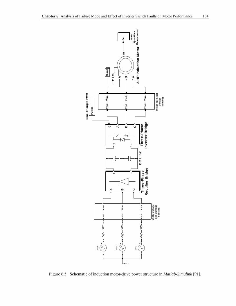
Chapter 6: Analysis of Failure Mode and Effect of Inverter Switch Faults on Motor Performance
134
DC
Lin
kV
sc
Vsb
Vsa
Vsa
+
Vsb
+
Vsc
+
Vsa
-
Vsb
-
Vsc
-
Util
ity V
olta
gean
d C
urre
ntS
ensi
ng
A B C
+ -
Thre
e-P
hase
Rec
tifie
r B
ridg
e
g A B C
+ - Thre
e-P
hase
Inve
rter
Bri
dge
TLoa
d
Pul
ses
Sine
-Tri
angl
e PW
M
Vm
a+
Vm
b+
Vm
c+
Vm
a-
Vm
b-
Vm
c-
Mot
or T
erm
inal
Vol
tage
Sen
sing
Out Mot
orQ
uant
ities
Mea
sure
men
t
Tm
mA B C
2-H
P In
duct
ion
Mot
or
Figure 6.5: Schematic of induction motor-drive power structure in Matlab-Simulink [91].

Chapter 6: Analysis of Failure Mode and Effect of Inverter Switch Faults on Motor Performance
135
Table 6.1: Simulation conditions of induction motor-drive system.
Utility Utility Input Voltage (Line-To-Line) 460 Volts Frequency 60 Hz Line Resistance (4.8%) 0.7082 Ω Line Inductance (4.8%) 1.8786 mH
DC Link (2 capacitors in series) Capacitance Value 2000 µF per capacitor
Induction Motor Rated Power 2 hp (1492 Watts) Rated Voltage (Line-To-Line) 460 Volts Rated Current 3.0 Amps Rated Frequency 60 Hz Rated Speed 1744 r/min Rated Torque 8.169 Nm Phase 3 Number of Poles 4 Stator Resistance, sR 3.850 Ω Rotor Resistance, rR 2.574 Ω Stator Leakage Inductance, lsL 17.5594 mH Rotor Leakage Inductance, lrL 17.5594 mH Magnetizing Inductance, mL 0.372674 H
Moment of Inertia, J 0.028 kg.m2
Load ( 2L L mT k ω= )
Load Coefficient, Lk -3 20.24493 10 Nm/(m. rad/s)×
PWM Controller Carrier-Based Sine-Triangle Modulation Index, ma 0.9 Switching Frequency 5 kHz

Chapter 6: Analysis of Failure Mode and Effect of Inverter Switch Faults on Motor Performance
136
6.3.1.2 Analytical and Simulation Results
The analytical waveforms of the three-phase motor line-to-neutral voltages obtained using
(6.16) and (6.17), under transistor short-circuit switch fault at S1, are shown here in Figure 6.6(a),
under the conditions of 0.9am = and 610 VoltsdcV = . This is in order to match with the
simulation operating conditions. Again, it should be noted that the complementary transistor
switch, S4, was turned-off in order to avoid a shoot-through. The corresponding simulation results
of the motor line-to-neutral voltages, at a low-pass filtering cutoff frequency of 120-Hz, are
depicted in Figure 6.6(b). The purpose of filtering the voltage waveforms is to be able to
meaningfully compare them with the analytical results that neglect the lower-order frequency
space/machine induced time harmonics, as well as the higher-order frequency time harmonics due
to the PWM switching. It can be observed from Figure 6.6 that the analytical waveforms are in
good agreement with the simulation waveforms. The FFT frequency spectra of the associated
simulated three-phase voltage waveforms are illustrated in Figure 6.7. The dc and the
fundamental harmonic voltage terms of all phases computed using (6.16) and (6.17), as well as
those obtained from the simulation frequency spectra of Figure 6.7 are given in Table 6.2. Again,
the analytical and simulation values match quite well with one another.
The simulation results of the three-phase motor currents during pre- and post-fault
conditions are depicted in Figure 6.8. As one can observe therein, a severe transient occurs at the
time instant when the fault is introduced at 1.3 sect = . As was expected from the earlier
analysis, a large positive dc (unidirectional) current is present in phase-a, and this dc current is
divided equally between phase-b and phase-c, as was shown in Figure 6.8. The FFT frequency
spectra of the corresponding motor phase currents during post-fault condition are illustrated in
Figure 6.9 for all three phases. Again, notice the large dc current components present in all
phases. To verify the earlier analysis, the dc current terms were acquired analytically using (6.18),
and they are given in Table 6.3, along with the simulation values obtained from Figure 6.9.

Chapter 6: Analysis of Failure Mode and Effect of Inverter Switch Faults on Motor Performance
137
Therein, the close agreement between the analytical and simulation results confirms or validates
the earlier analytical study.
To further investigate the motor performance during post-fault condition, the motor speed
and developed torque profiles are depicted in Figure 6.10(a) and Figure 6.11(a), respectively. The
associated FFT frequency spectra during post-fault condition are also shown in Figure 6.10(b)
and Figure 6.11(b), respectively. It can be observed from the speed profile, upon the occurrence
of fault at 1.3 sect = , that the braking torque introduced by the dc magnetic field causes the
speed to drop sharply. In addition, as mentioned above, the electromagnetic interactions between
the resultant stator dc field and the resultant rotor fundamental rotating field introduce a pulsating
torque, and subsequent speed ripples, at the fundamental power frequency. This phenomenon can
be observed from the FFT spectra as was illustrated in Figure 6.10(b) and Figure 6.11(b) for the
speed and torque profiles, respectively. Notice in the FFT spectrum of the torque profile shown in
Figure 6.11(b), the fundamental component of the pulsating torque has a peak value of 79Nm,
which is substantially high as compared to the average torque (8.2Nm) of the motor during the
pre-fault (healthy) state.
Evidently, the extent of the fault severity due to a short-circuit switch fault on the motor
performance has been shown to be severe. Hence, fault isolation along with remedial action need
to be performed in a minimum of elapse time in order to maintain, to the fullest extent, the
desirable motor performance characteristics during normal operation. This remedial action will be
detailed in the next chapter.

Chapter 6: Analysis of Failure Mode and Effect of Inverter Switch Faults on Motor Performance
138
Analytical
0 0.01 0.02 0.03 0.04 0.05-400
-300
-200
-100
0
100
200
300
400
Mot
or P
hase
Vol
tage
s (V
)
Time (sec)
VanVbnVcn
(a)
Simulation
2 2.01 2.02 2.03 2.04 2.05 -400
-300
-200
100
0
100
200
300
400
Mot
or P
hase
Vol
tage
s (V
)
Time (sec)
VanVbnVcn
(b)
Figure 6.6: Three-phase motor phase voltages during short-circuit switch fault condition. (a) Analytical. (b) Simulation.

Chapter 6: Analysis of Failure Mode and Effect of Inverter Switch Faults on Motor Performance
139
DC 1 2 3 4 5 6 7 8 9 100
50
100
150
200
250
Mag
nitu
de (V
)
Harmonic Order (a)
DC 1 2 3 4 5 6 7 8 9 100
50
100
150
200
250
Mag
nitu
de (V
)
Harmonic Order (b)
DC 1 2 3 4 5 6 7 8 9 100
50
100
150
200
250
Mag
nitu
de (V
)
Harmonic Order (c)
Figure 6.7: FFT spectra of simulated three-phase motor phase voltages during short-circuit switch fault condition. (a) Phase-a. (b) Phase-b. (c) Phase-c.
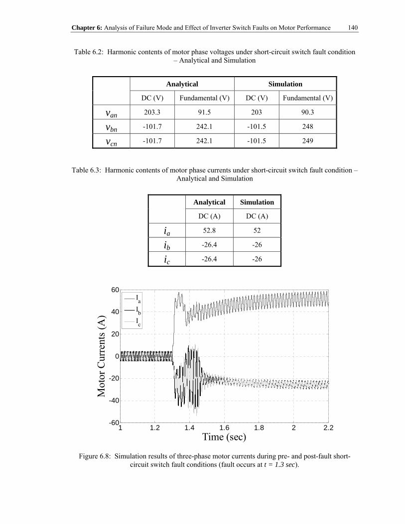
Chapter 6: Analysis of Failure Mode and Effect of Inverter Switch Faults on Motor Performance
140
Table 6.2: Harmonic contents of motor phase voltages under short-circuit switch fault condition – Analytical and Simulation
Analytical Simulation
DC (V) Fundamental (V) DC (V) Fundamental (V)
van 203.3 91.5 203 90.3
vbn -101.7 242.1 -101.5 248
vcn -101.7 242.1 -101.5 249
Table 6.3: Harmonic contents of motor phase currents under short-circuit switch fault condition – Analytical and Simulation
Analytical Simulation
DC (A) DC (A)
ia 52.8 52
ib -26.4 -26
ic -26.4 -26
1 1.2 1.4 1.6 1.8 2 2.2-60
-40
-20
0
20
40
60
Mot
or C
urre
nts (
A)
Time (sec)
IaIbIc
Figure 6.8: Simulation results of three-phase motor currents during pre- and post-fault short-circuit switch fault conditions (fault occurs at t = 1.3 sec).

Chapter 6: Analysis of Failure Mode and Effect of Inverter Switch Faults on Motor Performance
141
DC 1 2 3 4 5 6 7 8 9 100
10
20
30
40
50
60
Mag
nitu
de (A
)
Harmonic Order
DC Value = 52 A
Fundamental Value = 6.34 A
(a)
DC 1 2 3 4 5 6 7 8 9 100
10
20
30
40
50
60
Mag
nitu
de (A
)
Harmonic Order
DC Value = 26 A
Fundamental Value = 3.39 A
(b)
DC 1 2 3 4 5 6 7 8 9 100
10
20
30
40
50
60
Mag
nitu
de (A
)
Harmonic Order
DC Value = 26 A
Fundamental Value = 3.03 A
(c)
Figure 6.9: FFT spectra of simulated three-phase motor currents during short-circuit switch fault condition. (a) Phase-a. (b) Phase-b. (c) Phase-c.

Chapter 6: Analysis of Failure Mode and Effect of Inverter Switch Faults on Motor Performance
142
1 1.2 1.4 1.6 1.8 2 2.2-1000
-500
0
500
1000
1500
2000
Mot
or S
peed
(r/m
in)
Time (sec) (a)
DC 1 2 3 4 5 6 7 8 9 100
10
20
30
40
50
60
70
80
Mag
nitu
de (r
/min
)
Harmonic Order (b)
Figure 6.10: Simulation results of motor speed during short-circuit switch fault condition (fault occurs at t = 1.3 sec). (a) Time-domain profile during pre- and post-fault. (b) FFT spectrum
during post-fault.

Chapter 6: Analysis of Failure Mode and Effect of Inverter Switch Faults on Motor Performance
143
1 1.2 1.4 1.6 1.8 2 2.2-800
-600
-400
-200
0
200
400
600
800
Dev
elop
ed T
orqu
e (N
m)
Time (sec) (a)
DC 1 2 3 4 5 6 7 8 9 100
10
20
30
40
50
60
70
80
Mag
nitu
de (N
m)
Harmonic Order (b)
Figure 6.11: Simulation results of motor developed torque during short-circuit switch fault condition (fault occurs at t = 1.3 sec). (a) Time-domain profile during pre- and post-fault. (b)
FFT spectrum during post-fault.

Chapter 6: Analysis of Failure Mode and Effect of Inverter Switch Faults on Motor Performance
144
6.3.2 Open-Circuit Switch Fault
Failure in either one of the PWM digital output ports of a DSP board or one of the isolation
amplifiers of the gate drive can lead to an open-circuit fault in the transistor switch, as shown in
Figure 6.1. A transistor open-circuit switch fault is a less severe type of fault as compared to the
short-circuit switch fault. Nevertheless, such type of inverter fault will still generate disturbances
in the form of pulsating electromagnetic torque and a substantial dc component in the stator
winding currents. This dc current component will cause thermal problems, such as temperature
rise, in the windings. Eventually, insulation breakdown will occur if the fault is left unmitigated.
For the sake of analysis, an open-circuit fault occurring in switch, S1, is considered in this work.
A misfiring of the transistor switch, S1, will result in an inverter circuit topology, as
illustrated in Figure 6.12. Intuitively, through the observation of Figure 6.12, one can state that
there will not be any positive current flow into the motor for phase-a after the fault occurrence,
due to the absence or malfunction of switch S1. Hence, the resulting post-fault phase-a current, ai ,
will consist of a dc (unidirectional) current component. If the motor has an isolated (floating)
neutral connection, this dc (unidirectional) current term will be divided between the currents of
the remaining two phases. As previously mentioned, the consequence of having a dc
(unidirectional) current circulating in the motor windings leads to the significant presence of
motor torque pulsations.
In the circuit of Figure 6.12, the pole voltage of phase-a is determined based on the phase-a
current, ai , and the switching patterns associated with the switch, S4. If the switching patterns of
S4, as well as the other switches of phase-b and phase-c, remain the same after the fault
occurrence, the pole voltages, , ,ao bo cov v v , can be defined based on the earlier derivations of the
averaged switching functions, assuming that current is positive when flowing into the motor
terminal, as follows:

Chapter 6: Analysis of Failure Mode and Effect of Inverter Switch Faults on Motor Performance
145
2dcV
2dcV
Figure 6.12: Inverter circuit topology with an open-circuit fault at switch S1.
( )
( )
( )
4
4
for 0 State-12
for 0 and is ON State-22
for 0 and is OFF State-32
12
dca
dca
aodc
a
bo
V i
V i Sv
V i S
v
− >
− <=
<
+( ) ( )
( )
( )
3 for 0 State-4
1 cos 2 321 cos 4 32
co a a
bo a dc
co a dc
v e i
v m V t
v m V t
ω π
ω π
⎧⎪⎪⎪⎪⎨⎪⎪⎪⎪ + =⎩
= −
= −
(6.19)
where, ae represents the back emf of the phase-a motor winding.
As one can see from (6.19), there are four different states associated with the pole voltage of
phase-a. The first state, namely State-1, implies that 2ao dcv V= − when 0ai > . It should be
noted that this state only takes place when the phase-a current is positive during the time instant
of the fault occurrence. Hence, this state represents the time interval between the fault instant and
the first zero-crossing instant of the phase-a current, ai . During this time interval, the free-
wheeling diode, 4d , will conduct current.

Chapter 6: Analysis of Failure Mode and Effect of Inverter Switch Faults on Motor Performance
146
The next two states, namely State-2 and State-3, occur during the negative half cycle of the
phase-a current. In these states, the phase-a pole voltage, aov , alternates between 2dcV and
2dcV− , depending on the switching patterns. Accordingly, from the averaged switching
function derivation, the line-to-neutral voltages of all three phases can be defined as follows:
( )
( )
( )
1 cos21 cos 2 3 for State-2 and State-321 cos 4 32
an a dc
bn a dc
cn a dc
v m V t
v m V t
v m V t
ω
ω π
ω π
⎫= ⎪⎪⎪= − ⎬⎪⎪= − ⎪⎭
(6.20)
Notice that the three-phase voltages of (6.20) take the healthy form as given previously in (6.14).
The last state, namely State-4, takes place when ai is zero, owing to the inaction of switch
S1. Therefore, during this state, the motor phase-a line-to-neutral voltage is equal to its back emf,
that is, an av e= . By virtue of the following expressions, ao an nov v v= + and
( ) 3no ao bo cov v v v= + + , the pole voltage of phase-a is as defined in (6.19). That is,
( )3 2ao bo co av v v e= + + . Using (6.4), the line-to-neutral voltages of all three phases can be
expressed as follows:
( )
( )
1 for State-4212
an a
bn bo co a
cn co bo a
v e
v v v e
v v v e
⎫= ⎪⎪⎪= − − ⎬⎪⎪= − − ⎪⎭
(6.21)
It is important to point out that only State-2 through State-4 are still valid after the on-set of the
fault transient.

Chapter 6: Analysis of Failure Mode and Effect of Inverter Switch Faults on Motor Performance
147
1.27 1.28 1.29 1.3 1.31 1.32 1.33-400
-200
0
200
400
Van
(V) /
ea (V
) / I a (A
)
Time (sec)
VaneaIa*20
Figure 6.13: Simulation waveforms of motor quantities during pre- and post-fault conditions (open-circuit switch fault occurred at switch S1 at t = 1.3 sec).
Pictorial representations of the motor phase-a voltage ( anv ), back emf ( ae ), and current ( ai )
during pre- and post-fault conditions were obtained through simulation and are depicted in Figure
6.13. Here, the open-circuit switch fault occurred at switch S1 at t = 1.3 sec. Note that the phase
current, ai , is multiplied by a factor of 20 for better and clearer visualization. As one can observe
therein, the fault occurred when the current is negative. Hence, State-1 will never be in effect
during the post-fault period. In addition, when the current is equal to zero (State-4), the phase-a
voltage (shown by the solid line in Figure 6.13) is in congruence with its back emf (shown by the
dotted line), which is in agreement with the foregoing development as given in (6.21). Moreover,
in the same figure, during the negative half cycle of the motor phase current (State-2 and State-3),
the phase-a voltage, anv , reverts to its healthy form, which again corresponds to the earlier
development as delineated in (6.20). An important observation worth noting from Figure 6.13 is
the presence of the negative dc (unidirectional) offsets in both the phase current and voltage.
Notwithstanding this fact, these dc (unidirectional) offsets are smaller in magnitude than their

Chapter 6: Analysis of Failure Mode and Effect of Inverter Switch Faults on Motor Performance
148
respective fundamental components. Thus, the braking torque will have less significant effect.
Nevertheless, a pulsating torque, at the fundamental power cycle frequency, with significant
negative impact on motor performance will still be present.
6.3.2.1 Simulation Results
Simulation results are presented here to demonstrate the impact of the failure of an open-
circuit switch fault on the motor performance. The 2-hp induction motor-drive system under
study was simulated here in a Matlab-Simulink environment [91], see Figure 6.5, with the
associated simulation conditions which were given in Table 6.1. The open-circuit fault location is
assumed at switch, S1, and the fault occurrence was introduced at time, t = 1.3 sec. Meanwhile,
the controller is of the open-loop constant volts per hertz PWM type, and the motor operation was
simulated under full-load condition, that is at an output torque of 8.169 Nm.
The simulation waveforms of the three-phase motor currents during pre- and post-fault
conditions are plotted in Figure 6.14(a) and Figure 6.14(b), respectively. As one can observe from
the post-fault result of Figure 6.14(b), a malfunction (open-circuit) of the switch, S1, results in the
elimination of any positive current flow in phase-a of the stator windings of the motor.
Consequently, a dc (unidirectional) offset is imposed on the current of phase-a, and this dc
(unidirectional) current is divided between the paths of the remaining two phases, provided that
the motor has a floating neutral connection. It should also be noted that due to the unbalanced
voltage excitations at the motor terminals as a result of the fault, negative sequence components
will also be introduced in the motor currents.
Meanwhile, the corresponding FFT frequency spectra of the motor phase currents are shown
in Figure 6.15(a) for the healthy case, and Figure 6.15(b) through (d) for the faulty case. Despite
the presence of the dc (unidirectional) current offsets in all three phases, their magnitudes are
smaller than their respective fundamental components, as depicted in Figure 6.15(b) through (d).

Chapter 6: Analysis of Failure Mode and Effect of Inverter Switch Faults on Motor Performance
149
Hence, the possibility of a motor stall is unlikely, which is not the case for a transistor short-
circuit switch fault as was previously illustrated in this chapter. Observation of Figure 6.15(b)
through (d) also indicates the presence of lower-order time harmonics imposed on the motor
currents. This can best be explained by examining the simulation waveform of the dc link voltage
and its corresponding FFT spectra, as illustrated in Figure 6.16(a) and Figure 6.16(b) and its
close-up (zoom) depiction in Figure 6.16(c), respectively. In a healthy three-phase electric drive,
the dc link voltage is composed of a dc component, as well as higher-order harmonic frequency
components that are multiple of six. However, as a consequence of asymmetry in the inverter
circuit, lower-order harmonics are generated in the dc link, particularly the fundamental harmonic
component at the main power cycle frequency. This can be observed in both the time-domain
waveform, see Figure 6.16(a), and the close-up view of the FFT spectrum, see Figure 6.16(c),
respectively.
To demonstrate the effects of these dc link harmonics on the motor phase voltages and
currents, the previously derived averaged-switching-function model is invoked. Considering a dc
bus voltage with dc, 1st, and 2nd harmonic components, one can write the dc bus voltage
expression as follows:
( ) ( ) ( )0 1 21 2cos cos 2dc dc dc dcV t V V t V tω φ ω φ= + + + + (6.22)
where, 0dcV is the average dc bus voltage,
1dcV and 2dcV represent the peak magnitudes of the first
(fundamental) and second harmonic components, whereas, 1φ and 2φ , represent their respective
phase angles. By substituting (6.22) in (6.14), one can obtain the three-phase line-to-neutral
voltages, that is, anv , bnv , and cnv , as follows:

Chapter 6: Analysis of Failure Mode and Effect of Inverter Switch Faults on Motor Performance
150
( ) ( )( )
( )
( ) ( )( )
( )
( ) ( )( )
0 1 2
0 1 2
0 1 2
1 2
1 2
1 2
1 cos cos 2 cos2
1 cos cos 2 cos 2 32
1 cos cos 22
dc
dc
dc
an a dc dc dc
V t
bn a dc dc dc
V t
cn a dc dc dc
V t
v m V V t V t t
v m V V t V t t
v m V V t V t
ω φ ω φ ω
ω φ ω φ ω π
ω φ ω φ
⎡ ⎤= + + + +⎣ ⎦
⎡ ⎤= + + + + −⎣ ⎦
⎡ ⎤= + + + +⎣ ⎦ ( )cos 4 3tω π−
(6.23)
Using the trigonometric identity, ( ) ( ) ( ) ( )cos cos 1 2 cos 1 2 cosa b a b a b= ⋅ − + ⋅ + , one can
rewrite (6.23) in the following manner:
( ) ( ) ( )0 1
nd
1 1
dc Term Positive-SequencePositive-Sequence 2 Harmonic TermFundamental Term
1 1cos cos cos 22 4
an a dc a dcv m V t m V tω φ ω φ
⎡ ⎤⎢ ⎥
= + + +⎢ ⎥⎢ ⎥⎢ ⎥⎣ ⎦
( ) ( )
( )
2
rd
0 1
2 2
Negative-Sequence Positive-SequenceFundamental Term 3 Harmonic Term
Positive-SequenceFundamental Term
1 cos cos 34
1 1cos 2 3 co2 4
a dc
bn a dc a dc
m V t t
v m V t m V
ω φ ω φ
ω π
⎡ ⎤⎢ ⎥
+ + + +⎢ ⎥⎢ ⎥⎢ ⎥⎣ ⎦
= − + ( ) ( )
( )
nd
2
1 1
dc Term Positive-Sequence2 Harmonic Term
2
Negative-SequenceFundamental Te
s 2 3 cos 2 2 3
1 cos 2 34 a dc
t
m V t
φ π ω φ π
ω φ π
⎡ ⎤⎢ ⎥
+ + + −⎢ ⎥⎢ ⎥⎢ ⎥⎣ ⎦
+ + + ( )
( ) ( ) ( )
rd
0 1
2
Positive-Sequencerm 3 Harmonic Term
1 1
dc Term Positive-Positive-SequenceFundamental Term
cos 3 2 3
1 1cos 4 3 cos 4 3 cos 2 4 32 4cn a dc a dc
t
v m V t m V t
ω φ π
ω π φ π ω φ π
⎡ ⎤⎢ ⎥
+ + −⎢ ⎥⎢ ⎥⎢ ⎥⎣ ⎦
= − + + + + −
( ) ( )
nd
2
r
Sequence2 Harmonic Term
2 2
Negative-Sequence Positive-SequenceFundamental Term 3
1 cos 4 3 cos 3 4 34 a dcm V t tω φ π ω φ π
⎡ ⎤⎢ ⎥⎢ ⎥⎢ ⎥⎢ ⎥⎣ ⎦
+ + + + + −
d Harmonic Term
⎡ ⎤⎢ ⎥⎢ ⎥⎢ ⎥⎢ ⎥⎣ ⎦
(6.24)
The first term given in all three voltage expressions of (6.24) represents the fundamental positive-
sequence component which contributes to the fundamental (useful) magnetic flux distribution in
the airgap. The corresponding second and third terms of (6.24) represent a dc offset and a 2nd
harmonic positive-sequence term, respectively. These terms are resulting from the effect of the 1st

Chapter 6: Analysis of Failure Mode and Effect of Inverter Switch Faults on Motor Performance
151
harmonic component of the dc link voltage. The last two terms given in all three voltage
expressions of (6.24), which are due to the effect of the 2nd harmonic dc voltage term, represent a
fundamental negative-sequence term and a 3rd harmonic positive-sequence term, respectively.
Accordingly, the motor phase currents will be expected to consist of harmonic components
of corresponding nature to the order of harmonics that are given in (6.24). This is clearly
confirmed upon examination of the FFT spectra, as depicted in Figure 6.15(b) through (d).
Therein, the only harmonic term that is not shown in those spectral figures is the fundamental
negative-sequence component which leads to a flux component that is traveling in the airgap at an
angular synchronous frequency of ω− . It should be noted that the negative-sequence terms will
produce a negative torque (opposite to the motor’s rotation), which will reduce the overall
average torque of the motor. Also, one should not confuse the 3rd harmonic positive-sequence
term given in (6.24) with the traditional 3rd harmonic component referred to as common-mode or
zero-sequence component, where ( )3 3 3 3
cos 3a b c mi i i I tω= = = , in which case, along with the
other triple (9, 15, 21, 27,…,etc.) harmonic components, do not exist in this motor-drive fault
setup. This is due to the fact that the motor has a floating neutral point connection, constituting no
path for such harmonic currents. The remaining lower-order time harmonics of the motor phase
currents shown in the spectral Figure 6.15(b)-(d), that is harmonic components higher than the 3rd
order, can be explained in a similar manner using (6.22) and (6.23) by taking into account the
other higher harmonic terms of the dc link voltage.
The simulation results of the developed motor torque profile along with its corresponding
FFT spectra during pre- and post-fault conditions are given in Figure 6.17(a) and Figure 6.17(b)
and (c), respectively. The corresponding motor speed profile is also shown here in Figure 6.18.
As one can observe from the torque profile, see Figure 6.17(a), and speed profile, see Figure 6.18,
the effects of the presence of pulsations or ripples are clearly evident. These pulsations or ripples
are oscillating at a combination of several harmonic frequencies, with the main oscillating term

Chapter 6: Analysis of Failure Mode and Effect of Inverter Switch Faults on Motor Performance
152
being attributed to the fundamental harmonic term having a frequency equal to the power cycle
frequency. The cause of this torque component pulsating at synω can best be described through a
set of pictorial illustrations of the airgap flux and rotor magnetic field space-vectors, as depicted
in Figure 6.19. It should be noted that the harmonic components, including the dc component, of
the airgap flux and rotor magnetic field space-vectors are originating from the harmonic
components of the stator currents, the spectra of which are depicted in Figure 6.15. In
conventional machine theory, it is known that in an induction machine, the airgap flux and the
rotor magnetic field consist of harmonic components that are rotating at the same angular
frequency (angular synchronous speed). Hence, according to Figure 6.19(a), the relative speed
between the dc flux of the airgap and the fundamental positive-sequence harmonic component of
the rotor field, and vice versa, is synω . Therefore, both of these interactions will produce a torque
component that pulsates at the fundamental harmonic frequency, synω . On the other hand, in
Figure 6.19(b), the interactions between the dc airgap flux and the fundamental negative-
sequence harmonic component of the rotor field, and vice versa, will also produce a negative
pulsating torque at synω . Moreover, it can be seen from Figure 6.19(c) that the interactions
between the positive-sequence airgap fundamental flux and the 2nd harmonic component of the
rotor field, and vice versa, will also produce a positive torque pulsation at synω . The same
phenomenon can be stated with regard to the interactions between the positive-sequence 2nd and
3rd harmonic components of the airgap flux and the rotor field. Accordingly, the cumulative
effects of these electromagnetic interactions between the airgap flux and rotor field will result in a
torque component pulsating at synω . It should be noticed that the interactions between harmonic
components rotating at the same frequency produce a non-pulsating (or average) torque. A similar
argument can also be carried out to determine the cause of the other harmonic torque components
given in Figure 6.17(c). Meanwhile, it was calculated from the simulated torque profile of Figure

Chapter 6: Analysis of Failure Mode and Effect of Inverter Switch Faults on Motor Performance
153
6.17(a) that the peak-to-peak torque ripple is found to be about 190% of the post-fault average
torque. Clearly, this indicates that the continuous operation of the motor-drive system, upon the
occurrence of the fault, is highly undesirable in many applications. This is in order to avoid
mechanical damage to the motor bearings and shaft, as well as the mechanical load system.
In order to further investigate the motor performance due to an open-circuit switch fault, the
current space-vector locus, obtained by plotting id versus iq current components, under different
locations of the faulty transistor switch are plotted and shown here, along with the healthy case, in
Figure 6.20. It can be seen from these figures that the current space-vector locus under different
faulty switch locations exhibit different patterns, which are far from matching the circular locus
under healthy condition. Previous investigators have made use of these types of pattern indicators
to detect and locate the specific whereabouts of the open-circuit switch fault in an adjustable-
speed drive [76]-[82].

Chapter 6: Analysis of Failure Mode and Effect of Inverter Switch Faults on Motor Performance
154
1.95 1.96 1.97 1.98 1.99 2-8
-6
-4
-2
0
2
4
6
8
Mot
or C
urre
nts (
A)
Time (sec)
IaIbIc
(a)
1.95 1.96 1.97 1.98 1.99 2-8
-6
-4
-2
0
2
4
6
8
Mot
or C
urre
nts (
A)
Time (sec)
IaIbIc
(b)
Figure 6.14: Simulation results of three-phase motor currents during pre- and post-fault open-circuit switch fault conditions. (a) Healthy. (b) Post-Fault.

Chapter 6: Analysis of Failure Mode and Effect of Inverter Switch Faults on Motor Performance
155
DC 1 2 3 4 5 6 7 8 9 100
1
2
3
4
5M
agni
tude
(A)
Harmonic Order
(a) Healthy case in all phases.
DC 1 2 3 4 5 6 7 8 9 100
1
2
3
4
5
6
Mag
nitu
de (A
)
Harmonic Order
(b) Faulty case of ia.
DC 1 2 3 4 5 6 7 8 9 100
1
2
3
4
5
6
Mag
nitu
de (A
)
Harmonic Order
(c) Faulty case of ib.
DC 1 2 3 4 5 6 7 8 9 100
1
2
3
4
5
6
Mag
nitu
de (A
)
Harmonic Order
(d) Faulty case of ic.
Figure 6.15: FFT spectra of simulated three-phase motor currents during open-circuit switch fault condition. (a) Healthy case in all phases. (b) Faulty case of ia. (c) Faulty case of ib. (d) Faulty
case of ic.
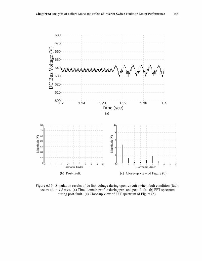
Chapter 6: Analysis of Failure Mode and Effect of Inverter Switch Faults on Motor Performance
156
1.2 1.24 1.28 1.32 1.36 1.4600
610
620
630
640
650
660
670
680
DC
Bus
Vol
tage
(V)
Time (sec) (a)
DC 1 2 3 4 5 6 7 8 9 100
100
200
300
400
500
600
700
Mag
nitu
de (V
)
Harmonic Order
(b) Post-fault.
DC 1 2 3 4 5 6 7 8 9 100
2
4
6
8
10
Mag
nitu
de (V
)
Harmonic Order
(c) Close-up view of Figure (b).
Figure 6.16: Simulation results of dc link voltage during open-circuit switch fault condition (fault occurs at t = 1.3 sec). (a) Time-domain profile during pre- and post-fault. (b) FFT spectrum
during post-fault. (c) Close-up view of FFT spectrum of Figure (b).

Chapter 6: Analysis of Failure Mode and Effect of Inverter Switch Faults on Motor Performance
157
1.2 1.24 1.28 1.32 1.36 1.4-5
0
5
10
15
20
Dev
elop
ed T
orqu
e (N
m)
Time (sec) (a)
DC 1 2 3 4 5 6 7 8 9 100
2
4
6
8
10
Mag
nitu
de (N
m)
Harmonic Order
(b) Pre-fault.
DC 1 2 3 4 5 6 7 8 9 100
2
4
6
8
10
Mag
nitu
de (N
m)
Harmonic Order
(c) Post-fault.
Figure 6.17: Simulation results of motor developed torque during open-circuit switch fault condition (fault occurs at t = 1.3 sec). (a) Time-domain profile during pre- and post-fault. (b)
FFT spectrum during pre-fault. (c) FFT spectrum during post-fault.

Chapter 6: Analysis of Failure Mode and Effect of Inverter Switch Faults on Motor Performance
158
1.2 1.24 1.28 1.32 1.36 1.41600
1650
1700
1750
1800
Mot
or S
peed
(r/m
in)
Time (sec)
Figure 6.18: Simulation results of motor speed during pre- and post-fault open-circuit switch fault conditions (fault occurs at t = 1.3 sec).
(rotor speed)mω
synω
synω
Airgap Fluxes⎫⎬⎭
Rotor Fields⎫⎬⎭
(a)
(rotor speed)mω
synω
synω
Airgap Fluxes⎫⎬⎭
Rotor Fields⎫⎬⎭
(b)
(rotor speed)mω
2 synω3 synω
2 synω3 synω
Airgap Fluxes⎫⎪⎬⎪⎭
Rotor Fields⎫⎪⎬⎪⎭
synω
synω
(c)
Figure 6.19: The origination of torque pulsations at a frequency, ωsyn. (a) Interactions between dc flux/field and positive-seq. 1st harmonic. (b) Interactions between dc flux/field and negative-
seq. 1st harmonic. (c) Interactions between positive-seq. 1st, 2nd, and 3rd harmonics.

Chapter 6: Analysis of Failure Mode and Effect of Inverter Switch Faults on Motor Performance
159
-10 -5 0 5 10-10
-5
0
5
10
I d (A)
Iq (A) (a) Healthy.
-10 -5 0 5 10-10
-5
0
5
10
I d (A)
Iq (A) (b) Open-circuit fault at S1.
-10 -5 0 5 10-10
-5
0
5
10
I d (A)
Iq (A) (c) Open-circuit fault at S4.
-10 -5 0 5 10-10
-5
0
5
10
I d (A)
Iq (A) (d) Open-circuit fault at S3.
-10 -5 0 5 10-10
-5
0
5
10
I d (A)
Iq (A) (e) Open-circuit fault at S6.
-10 -5 0 5 10-10
-5
0
5
10
I d (A)
Iq (A) (f) Open-circuit fault at S5.
-10 -5 0 5 10-10
-5
0
5
10
I d (A)
Iq (A) (g) Open-circuit fault at S2.
Figure 6.20: Simulation results of current space-vector locus.

Chapter 6: Analysis of Failure Mode and Effect of Inverter Switch Faults on Motor Performance
160
6.4 Summary
The main purpose of this chapter was to contribute to a better understanding of the impact of
various inverter faults, more specifically transistor/switch failures, on motor performance using a
combination of time-domain simulations and analytical derivations based on averaged switching
function modeling concepts. The two distinct types of inverter failure modes investigated herein
are: (1) a transistor short-circuit switch fault, and (2) a transistor open-circuit switch fault. In the
event of a short-circuit switch fault, the complementary switch of the same inverter leg has to be
instantaneously turned-off upon the on-set of such a fault in order to avoid the catastrophic event
of a dc link shoot-through situation. The resulting inverter circuit reconfiguration was accordingly
investigated. It was found from the study that the short-circuit switch fault produces a severe fault
impact on the motor performance. A dc (unidirectional) offset of high magnitude is imposed on
the motor current of each phase, which results in a braking torque that causes the motor speed to
drop sharply. In addition, huge torque pulsations are also generated as a result of such an event.
Moreover, the presence of a high magnitude circulating dc (unidirectional) current in the motor
windings will eventually lead to insulation failure if the motor is left unattended. As a
consequence, such a fault will require immediate shut-down of the motor-drive system in order to
prevent secondary failures.
On the other hand, it was demonstrated here that an open-circuit switch fault will still permit
the operation of the motor-drive system, but at a much inferior performance due to the presence
of significant torque pulsations. It was found from this specific simulation case study that the
peak-to-peak torque pulsations were computed to be about 190% of the post-fault average torque
for the case-study 2-hp motor. This clearly indicates that the operation of the motor-drive system,
after the fault occurrence, can only be extended for a short period of time. This is in order to
avoid damages to the mechanical portions of the motor-drive system. Analytical studies were also

Chapter 6: Analysis of Failure Mode and Effect of Inverter Switch Faults on Motor Performance
161
presented in this work to determine the causes of these torque pulsations. In the opinion of this
investigator, a detailed understanding of these fault impacts on machine performance is essential
when one proceeds to the design stage of developing remedial strategies for such types of faults,
which will be presented in the forthcoming chapter.

162
CHAPTER 7
7 A QUASI-CYCLOCONVERTER-BASED
TOPOLOGY AND CONTROL FOR
INVERTER FAULT MITIGATION
7.1 Introduction
The main idea leading to the development of the present approach as a potential solution for
motor-drive inverter switch fault mitigation was attributed to a discovery by this investigator,
while implementing the control algorithm of soft starters in the earlier work. Therein, it was
discovered by this investigator that proper control of the SCRs of the previously given topology
of a soft-starter, see Figure 7.1, in a specific switching pattern can produce a set of three-phase
positive-sequence voltages with a fundamental frequency other than the input supply frequency.
It was this specific discovery that led this investigator to conceive of the notion that such a
finding may serve as a potential remedial solution for inverter faults, by connecting the three-
phase SCR bridge whose configuration is shown in Figure 7.1 in parallel with the drive. In the
event of a fault, the drive will shut down by its own fault protection system, and the SCR bridge
will bypass the faulty drive to continue operation of the motor using the present control method.

Chapter 7: A Quasi-Cycloconverter-Based Topology and Control for Inverter Fault Mitigation
163
a
b
cn
AC Motor
iaVsa
Vsb
Vsc
ib
ic
Figure 7.1: SCR voltage-controlled topology.
(a) Proposed by Bolognani et al. [40].
(b) Proposed by Van Der Broeck et al. [52] and
Ribeiro et al. [44].
(c) Proposed by Liu et al. [49] and Elch-Heb et al. [50].
Figure 7.2: Different types of existing fault tolerant inverter topologies.

Chapter 7: A Quasi-Cycloconverter-Based Topology and Control for Inverter Fault Mitigation
164
This idea of fault mitigation appeared to this investigator to be promising, in light of a
thorough investigation which was carried out on the existing fault tolerant solutions that were
previously proposed by other researchers [38]-[59], and which were discussed in detail earlier in
Chapter 1. For the convenience of the reader, these topologies proposed by earlier investigators
are depicted here in Figure 7.2. As mentioned earlier in Chapter 1, each of the topologies of
Figure 7.2 has its own merits and drawbacks. The merit of these topologies is their ability to
maintain continuous operation of the machine in the event of an inverter fault. On the other hand,
the drawbacks range from having the need for a redundant inverter leg for the topology of Figure
7.2(a), oversizing the dc capacitors and doubling the dc link voltage for the topology of Figure
7.2(b), to the need for a motor neutral connection as well as oversizing the dc link capacitors for
the topology of Figure 7.2(c).
Examination of those inverter topologies reveals one common thing. Namely that is the
mechanism, which enables the change in the status of the inverter into its post-fault configuration
in order to allow the fault mitigation control to be applied thereafter, consists of three sets of
back-to-back connected SCRs which resembles the configuration shown in Figure 7.1.
Accordingly, in comparison with the existing topologies of Figure 7.2, the present remedial
approach, based on the SCR bridge configuration of Figure 7.1, will not introduce any additional
cost on top of what had already been proposed by others in Figure 7.2. However, it will be
demonstrated later on that in order for the motor to operate at more selectable frequencies,
additional two sets of back-to-back connected SCRs are essential, resulting in a total of five sets
of back-to-back connected SCRs, as depicted in Figure 7.3. Nevertheless, the present approach is
still worth the effort for achieving a potential remedial solution for the case of inverter faults.
In fact, the present fault mitigation approach has the following attributes: (1) does not
require the accessibility of the neutral point of the motor which is normally not provided by motor
manufacturers except by special request, (2) does not need to double the dc bus voltage which can

Chapter 7: A Quasi-Cycloconverter-Based Topology and Control for Inverter Fault Mitigation
165
only be realized through either a dc-dc boost converter or an active rectifier at the drive front-end,
and (3) does not need to oversize the dc link capacitors in order to sustain the desired voltage
level and minimize the voltage ripples due to the single-phase current circulating through the
capacitors. Another appealing feature of this new approach is its ability of potential use for
mitigating any other drive-related faults such as faults occurring in the diode rectifier bridge or
the dc-link capacitor because of the fact that this approach bypasses the entire drive system,
provided that such faults can be safely isolated. Despite the aforementioned merits, due to its
unique control operation, the present topology is only suitable for low-speed type of motor
applications, such as vehicle and ship propulsion systems, cement mills, mine hoists, rolling mills
and the like, where high torque at low speed is indispensable [101]. In addition, the appearance of
a pulsating torque will be evident from the motor performance as a result of the present approach.
Details of these will be explained further later-on in this chapter.
In light of the present topology structure and its operating principles, one can consider it as
an ac-to-ac frequency changer, or “cycloconverter”. The basic function of a cycloconverter is to
convert directly the incoming supply frequency to some different output frequency [99]. For most
practical purposes, the maximum attainable useful output frequency is less than the input
frequency. Hence, this is a fundamental limitation of a cycloconverter. The operation of a
cycloconverter is carried out by controlling the switching patterns of a plurality of static SCR
switches connected directly between the input ac system and the motor [99]. Unlike the standard
PWM drives, there is basically no energy storage element present in the converter. In real
applications, the cycloconverter is generally adopted for high power drive applications, in the
range of MegaWatts, such as power mills for grinding purposes in mineral processing plants
[102]. This is because of the high voltage and high current withstand ratings of SCR switches. A
typical three-phase cycloconverter consists of 6 SCR switches for each phase, resulting in a total
of 18 SCR switches. Hence, the present topology of Figure 7.3, with a total of 10 SCRs, can be
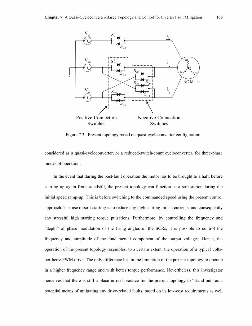
Chapter 7: A Quasi-Cycloconverter-Based Topology and Control for Inverter Fault Mitigation
166
b
a
cn
AC Motor
iaVsa
Vsb
Vsc
ib
ic
1AS +
2AS +
1BS +
2BS +
1CS +
2CS +
3BS −
4BS −3CS −
4CS −
Positive-ConnectionSwitches
Negative-ConnectionSwitches
Figure 7.3: Present topology based on quasi-cycloconverter configuration.
considered as a quasi-cycloconverter, or a reduced-switch-count cycloconverter, for three-phase
modes of operation.
In the event that during the post-fault operation the motor has to be brought to a halt, before
starting up again from standstill, the present topology can function as a soft-starter during the
initial speed ramp-up. This is before switching to the commanded speed using the present control
approach. The use of soft-starting is to reduce any high starting inrush currents, and consequently
any stressful high starting torque pulsations. Furthermore, by controlling the frequency and
“depth” of phase modulation of the firing angles of the SCRs, it is possible to control the
frequency and amplitude of the fundamental component of the output voltages. Hence, the
operation of the present topology resembles, to a certain extent, the operation of a typical volts-
per-hertz PWM drive. The only difference lies in the limitation of the present topology to operate
in a higher frequency range and with better torque performance. Nevertheless, this investigator
perceives that there is still a place in real practice for the present topology to “stand out” as a
potential means of mitigating any drive-related faults, based on its low-cost requirements as well

Chapter 7: A Quasi-Cycloconverter-Based Topology and Control for Inverter Fault Mitigation
167
as other merits that were previously mentioned above. Accordingly, the present topology with its
unique operation can be considered as a high-performance soft-starter and a moderate-
performance drive. Such technology is well-suited for users who are unwilling to bear the burden
of the high price of a typical PWM drive, and still hope to achieve with reduced requirements the
performance of variable speed operation at a lower affordable cost. In the following, the basic
principles of operation of the present topology and its control technique are set forth in detail.
7.2 Present Fault Mitigation Topology and Control
7.2.1 Operating Principle of Present Topology
The present solution for mitigating inverter faults is based on the topology given earlier in
Figure 7.3, and is re-illustrated here in Figure 7.4 with the inclusion of a standard PWM drive. In
this configuration, besides the PWM drive, the three-phase motor terminals are connected to the
ac supply mains terminals through a group of back-to-back connected SCRs. These SCRs are
segregated into two sets. The first set, namely “positive-connection switches”, consists of SCRs
that were labeled as 1BS + , 2BS + , 1CS + , and 2CS + . On the other hand, the second set of SCRs, namely
“negative-connection switches”, were labeled as 3BS − , 4BS − , 3CS − , and 4CS − . Notice that including
the operation of the 1AS + and 2AS + set, the phase sequencing of the first set yields an abc positive
sequence switching. Meanwhile, including the operation of the 1AS + and 2AS + set, the phase
sequencing of the second set yields an acb negative sequence switching. The main objective of
having positive-connection switches as well as negative-connection switches is not to achieve
forward or backward rotation control of the motor. In fact, its purpose is to provide a speed
control at more selectable frequencies such that the sequence of the fundamental components of
the voltages received at the motor terminals shall always possess a positive-sequence orientation
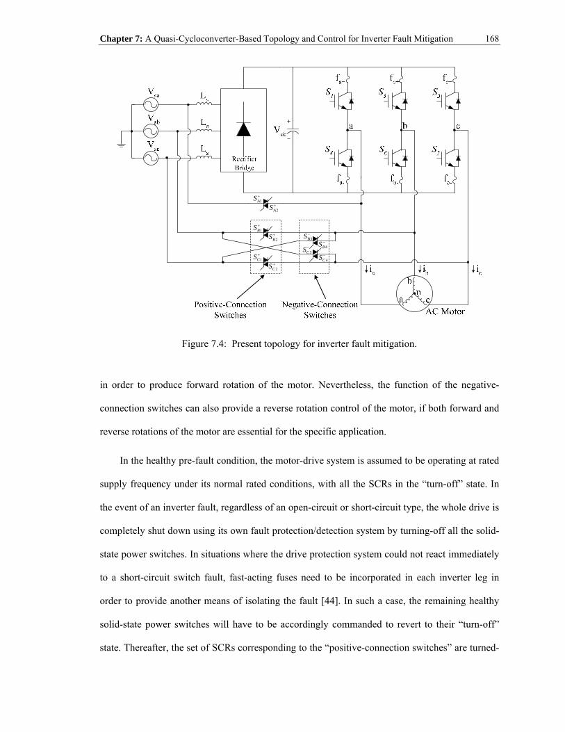
Chapter 7: A Quasi-Cycloconverter-Based Topology and Control for Inverter Fault Mitigation
168
1AS +
2AS +
1BS +
2BS +
1CS +
3BS −
4BS −
3CS −
4CS −
2CS +
Figure 7.4: Present topology for inverter fault mitigation.
in order to produce forward rotation of the motor. Nevertheless, the function of the negative-
connection switches can also provide a reverse rotation control of the motor, if both forward and
reverse rotations of the motor are essential for the specific application.
In the healthy pre-fault condition, the motor-drive system is assumed to be operating at rated
supply frequency under its normal rated conditions, with all the SCRs in the “turn-off” state. In
the event of an inverter fault, regardless of an open-circuit or short-circuit type, the whole drive is
completely shut down using its own fault protection/detection system by turning-off all the solid-
state power switches. In situations where the drive protection system could not react immediately
to a short-circuit switch fault, fast-acting fuses need to be incorporated in each inverter leg in
order to provide another means of isolating the fault [44]. In such a case, the remaining healthy
solid-state power switches will have to be accordingly commanded to revert to their “turn-off”
state. Thereafter, the set of SCRs corresponding to the “positive-connection switches” are turned-

Chapter 7: A Quasi-Cycloconverter-Based Topology and Control for Inverter Fault Mitigation
169
on (whereas, the SCRs associated with the “negative-connection switches” are turned-off) for a
normal forward rotating mode, which leads to the bypass transfer whereupon the motor is fed
directly from the ac supply mains. In order to maintain synchronization and to avoid any
interruption at the point of bypass transfer, the reference (modulating) waveforms employed in
the pulse-width modulation scheme of the drive have to be in synchronism with the ac supply
mains voltages using a phase-locked loop (PLL) scheme [100]. Again, it should be emphasized
that regardless of which set of switches are in action, the SCRs of phase-a, namely 1AS + and 2AS + ,
will always be a part of the switching process, in order to provide a balanced three-phase
operation.
In order to realize fault tolerant operation in the adjustable-speed mode, besides the rated
frequency of the ac supply mains, a discrete-frequency control method is utilized here. Due to its
unique control scheme, the present approach is only suitable for low-speed motor applications. It
had been discovered by this investigator that selectively triggering of the SCRs in a specific
pattern can produce a set of three-phase voltages, and consequently three-phase currents, having a
fundamental output frequency, of , which is an integer fraction of the frequency of the ac supply
mains, sf . That is, the output frequency, ( )1 2o sf f= , ( )1 4 sf , ( )1 5 sf , ( )1 7 sf , ( )1 8 sf ,
( )1 10 sf ,...,etc. In other words, o sf f N= , where, N = 2, 4, 5, 7, 8, 10, 11, 13, 14, 16, 17, 19,
20, 22, 23, 25,…, etc. Notice that frequencies where N = 3, 6, 9, 12, 15,…, etc. are unavailable
for reasons explained below.
A set of example current patterns at selected frequencies down to ( )1 8 sf are graphically
illustrated in Figure 7.5. As one can observe therein, by triggering the SCRs in a specific pattern
to produce a set of current pulses, one can obtain fundamental frequencies, as shown by the
dotted lines of Figure 7.5, that are lower than the ac supply mains frequency, sf . Hence, this
resembles very much the performance of a cycloconverter, which is the reason for referring to the

Chapter 7: A Quasi-Cycloconverter-Based Topology and Control for Inverter Fault Mitigation
170
60 30Hz2of = =
60 15Hz4of = =
60 12Hz5of = =
60 8.57Hz7of = =
60 7.5Hz8of = =
60Hzsf =
Figure 7.5: Example current patterns using discrete-frequency control for adjustable-speed mode operation for a supply mains frequency, 60Hzsf = .
present topology as a quasi-cycloconverter-based topology. Since the available frequencies
resulting from this discrete-frequency control method are equal to or lower than half the rated
supply frequency, the present fault tolerant approach is mainly applicable to situations where low
speed operation is acceptable such as in emergency “limp-home” situations in vehicles and other
propulsion applications.
The importance of having two separate sets of SCRs, see Figure 7.3 and Figure 7.4, is
explained in the following discussion. Assuming a set of balanced, three-phase positive-sequence,
one per-unit waveforms, to be expressible as follows:
( ) ( )( ) ( )( ) ( )
cos
cos 2 3
cos 4 3
A o
B o
C o
v t t
v t t
v t t
ω
ω π
ω π
=
= −
= −
(7.1)

Chapter 7: A Quasi-Cycloconverter-Based Topology and Control for Inverter Fault Mitigation
171
where, 2o ofω π= , is the commanded output angular frequency, one can express the ac supply
mains angular frequency, 2s sfω π= , and o s Nω ω= . Here, N is the set of acceptable integers
given above. Consequently, using (7.1), one can express a set of balanced, three-phase supply
mains voltages at the angular frequency, sω , in the following manner:
( ) ( ) ( )( ) ( ) ( )( ) ( ) ( )
cos cos
cos 2 3 cos 2 3
cos 4 3 cos 4 3
sa m o m s
sb m o m s
sc m o m s
v t V N t V t
v t V N t V t N
v t V N t V t N
ω ω
ω π ω π
ω π ω π
= =
= − = −⎡ ⎤⎣ ⎦= − = −⎡ ⎤⎣ ⎦
(7.2)
where, mV is the voltage peak (maximum) amplitude of the ac supply mains. As one can observe
in (7.2), the lag phase angles for phase-b and phase-c of the supply mains voltages determine the
overall voltage sequence order, whether it is an (abc) positive or an (acb) negative sequence. In
other words, for positive-sequence order, 3 1N k= + ; while for negative-sequence order,
3 2N k= + ; and for zero-sequence order, 3 3N k= + , where k = 0, 1, 2, 3, 4, 5,…,etc. Hence,
this implies that in order to produce a set of three-phase, positive-sequence output voltage
waveforms at an output frequency, o sf f N= , the sequence order of the ac supply mains needs
to be varied depending on the commanded output frequency, of . It is always considered in any
situation that the supply mains voltages always preserve a positive-sequence manner. Therefore,
in order to obtain a negative-sequence order of voltages from the ac supply mains, two phases of
the ac supply mains need to be interchanged. This can be realized using the set of “negative-
connection switches” for shifting the phase order of the ac supply mains, as depicted in both
Figure 7.3 and Figure 7.4. Clearly, it serves no purpose to achieve a zero-sequence order of
voltages from the ac supply mains for motor rotation. Hence, the available output frequencies that
can be obtained from using the proposed discrete-frequency control method can only be realized
for N = 2, 4, 5, 7, 8, 10, 11, 13, 14, 16, 17, 19, 20…,etc. This means that for the low-speed type of

Chapter 7: A Quasi-Cycloconverter-Based Topology and Control for Inverter Fault Mitigation
172
motor applications, there is a wider range of frequency to be selected, excluding N being a
multiple of “3”, which would lead to zero-sequence type abc voltages.
In order to re-emphasize the above concept, a graphical illustration is given in Figure 7.6(a)
and Figure 7.6(b) for 15-Hz and 30-Hz output waveforms, respectively. As shown in both figures,
the output waveforms have an amplitude of two per-units for clarity of demonstration purposes,
and they are labeled as Av , Bv , and Cv . Meanwhile, the input supply mains have an amplitude of
one per-units also for clarity of demonstration purposes, and they are labeled as sav , sbv , and scv .
It can be seen from both figures that the output waveforms at either 15-Hz or 30-Hz frequency are
shown in a positive-sequence manner. On the other hand, the 60-Hz supply mains are shown in a
positive-sequence manner for the case of 15-Hz output (that is N = 4), and a negative-sequence
manner for the case of 30-Hz output (that is N = 2). That is, for N = 4, the ac supply has to appear
to the motor through the SCR bridge in its (abc) positive-sequence form to provide a positive-
sequence output set of voltages at the commanded frequency, of . Meanwhile, for N = 2, the ac
supply has to appear to the motor through the SCR bridge in its (acb) negative-sequence form to
provide a positive-sequence output set of voltages at the commanded frequency, of .
7.2.2 Discrete-Frequency Control Algorithm
The main objective behind this discrete-frequency control approach is to selectively trigger
or turn-on the SCRs in a specific pattern in order to achieve the desired output waveforms at the
commanded frequency, o sf f N= . To demonstrate this concept, the switching patterns (trigger
signals) for the SCRs, 1AS + and 2AS + , of phase-a at commanded output frequencies of 30-Hz (N =
2), 15-Hz (N = 4), and 12-Hz (N = 5) are shown in Figure 7.7(a), (b), and (c), respectively. As one
may observe therein, each output frequency requires a different switching pattern for the turn-on
of the SCRs in order to realize the desired motor current pattern. Furthermore, each of the SCR

Chapter 7: A Quasi-Cycloconverter-Based Topology and Control for Inverter Fault Mitigation
173
firing pulses is phase-delayed by an angle, α , with respect to the zero-crossing of the supply
voltage before the corresponding SCR is triggered/turned-on. The choice of the value of α
depends on the motor load condition, with lower values for heavier loads. It should also be noted
that the angle, α , dictates the fundamental amplitude of the output voltage waveforms. Hence,
by adjusting the frequency of the triggering pulse as well as the value of the angle, α , one can
control both the frequency and amplitude of the output voltages impressed upon the motor to
render the performance of the bridge resembling the operating principle of a constant volts-per-
hertz control of a standard adjustable-speed drive.
The block diagram of the discrete-frequency control algorithm is depicted in Figure 7.8. The
desired output voltage frequency, of , applied at the motor terminals at integer fractions of the
supply mains frequency, sf , is first commanded, see Figure 7.8. Thereafter, a set of three-phase
positive-sequence waveforms, refv , at the commanded output frequency, o sf f N= , is
synthesized as a result. Again, notice that N is an integer that is not a multiple of 3. Hence, N = 2,
4, 5, 7, 8, 10, 11, 13, 14,…,etc. This set of three-phase waveforms, refv , is used as reference
waveforms for generating a set of positive-sequence voltages applied at the motor terminals. In
order to ensure a proper sequencing of the triggering pulses during low-speed operation, these
reference waveforms have to be in synchronism with the ac supply mains voltages in such a way
that the reference waveforms have the same zero crossings as the corresponding supply voltages,
as shown previously in Figure 7.6. This is carried out by sensing the ac supply mains voltages,
sav , sbv , and scv , and applying the PLL routine to attain the three angles of the supply voltages
for all three phases, that is aθ , bθ , and cθ [100]. With these set of angles, aθ , bθ , and cθ , and
the commanded frequency, of , the reference waveforms, refv , for each of the phases, a, b, and c,
can be synthesized accordingly.

Chapter 7: A Quasi-Cycloconverter-Based Topology and Control for Inverter Fault Mitigation
174
0 0.02 0.04 0.06 0.08 0.1 0.12 0.14-2
0
2
0 0.02 0.04 0.06 0.08 0.1 0.12 0.14-2
0
2
0 0.02 0.04 0.06 0.08 0.1 0.12 0.14-2
0
2
Time (sec)
(15Hz)Av
(15Hz)Bv
(15Hz)Cv
sav
sbv
scv
(a)
0 0.02 0.04 0.06 0.08 0.1 -2
0
2
0 0.02 0.04 0.06 0.08 0.1 -2
0
2
0 0.02 0.04 0.06 0.08 0.1 -2
0
2
Time (sec)
30-Hz Cycle 60-Hz Cycle
Phase-a
Phase-b
Phase-c
(30Hz)Av
(30Hz)Bv
(30Hz)Cv
sav
sbv
scv
(b)
Figure 7.6: Graphical illustrations on the sequence order of input supply mains to achieve output waveforms with different frequency. (a) 15-Hz output. (b) 30-Hz output.

Chapter 7: A Quasi-Cycloconverter-Based Topology and Control for Inverter Fault Mitigation
175
sav
ai
1AS +
2AS +
α α
(a)
sav
ai
1AS +
2AS +
αα
(b)
sav
ai
1AS +
2AS +
α α
(c)
Figure 7.7: Firing sequence of the SCRs of phase-a. (a) 30-Hz operation. (b) 15-Hz operation. (c) 12-Hz operation.

Chapter 7: A Quasi-Cycloconverter-Based Topology and Control for Inverter Fault Mitigation
176
α
o sf f N=, ,a b cθ θ θ
Figure 7.8: Block diagram of proposed control scheme for variable-speed operation.
To generate the proper sequencing of the triggering pulses for the SCRs, a phase-delayed
pulse generator was conceived. The input requirements for this phase-delayed pulse generator,
see Figure 7.8, are the three-phase reference waveforms for phases-a, b, and c, the angle, α , and
the zero-crossing time instants of all three phases of the supply voltages. The control logic (flow-
chart) of the phase-delayed pulse generator for phase-a of the present topology is illustrated in
Figure 7.9. The same control logic is also applied to phase-b and phase-c. It first begins by
sensing the phase-a supply mains, sav , and applying the zero-crossing detection scheme to the
measured signal. When a zero crossing of the voltage, sav , is detected, a phase-delayed angle
counter will be initiated to begin counting. Once the phase-delayed angle counter has reached the
value of the angle, α , a single firing pulse is generated by either the positive pulse generator or
the negative pulse generator depending upon the nature of the zero crossing. If the zero crossing
occurs during the instant when the polarity of the voltage changes from negative to positive, the
positive pulse generator will be selected, and vice versa. Once a train of pulses has been
generated, the last and crucial step is to decide the proper instant of triggering the SCRs, 1AS + and
2AS + . This is carried out by monitoring the polarity of the reference waveform, refv , for phase-a.
If 0refv > , the firing pulse generated by the positive pulse generator is sent to the gate of 1AS + for

Chapter 7: A Quasi-Cycloconverter-Based Topology and Control for Inverter Fault Mitigation
177
the turn-on, while 2AS + remains off. On the contrary, if 0refv < , 2AS + will be turned-on by the
firing pulse generated by the negative pulse generator, and 1AS + will be in its turn-off state. A
simple graphical illustration for the case of the 15-Hz output waveform is shown in Figure 7.10.
As may be observed in this figure, a train of pulses is generated by both the positive and negative
pulse generators, after a phase-delay by an angle, α , with respect to the zero crossings of the
supply voltage. Depending upon the polarity of refv of phase-a, the SCRs, 1AS + and 2AS + , are
selectively triggered accordingly, to produce a 15-Hz output waveform. Meanwhile, the same
control logic is also applicable for phase-b and phase-c of the SCRs shown in Figure 7.4 using
refv of phase-b and phase-c, respectively. The only difference lies in the selection of either the
positive-connection switches or the negative-connection switches, the decision of which is
depending upon the commanded output frequency. According to the aforementioned criteria, the
positive-connection switches are selected for N = 4, 7, 10, 13, 16, 19, 22,…, (3k+1), whereas the
negative-connection switches are selected for N = 2, 5, 8, 11, 14, 17, 20,…, (3k+2), where, k = 0,
1, 2, 3, 4, 5,…, etc.
As illustrated in Figure 7.5 or Figure 7.7, the three-phase motor currents obtained using the
present discrete-frequency control approach exhibit non-sinusoidal waveforms, which will entail
some torque pulsations in the motor performance, as will be elaborated later-on in simulation and
test results in the next chapter. Nevertheless, the average torque at the desired motor operating
condition will still be maintained.
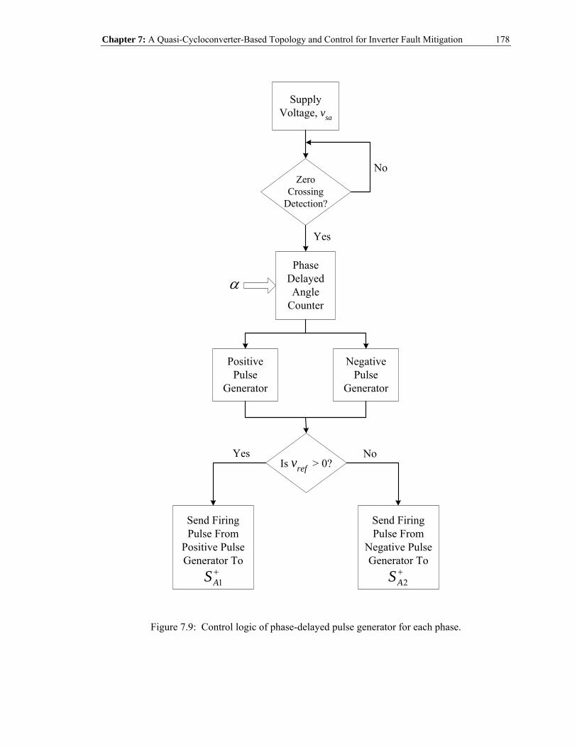
Chapter 7: A Quasi-Cycloconverter-Based Topology and Control for Inverter Fault Mitigation
178
Send FiringPulse From
Positive PulseGenerator To
1AS +
α
PositivePulse
Generator
NegativePulse
Generator
SupplyVoltage, vsa
ZeroCrossing
Detection?
No
Yes
PhaseDelayedAngle
Counter
Is vref > 0?NoYes
Send FiringPulse From
Negative PulseGenerator To
2AS +
Figure 7.9: Control logic of phase-delayed pulse generator for each phase.

Chapter 7: A Quasi-Cycloconverter-Based Topology and Control for Inverter Fault Mitigation
179
sav
1AS +
2AS +
α
refv
Figure 7.10: Graphical illustration of the control logic to achieve 15-Hz operation.
7.3 Summary
In summary, a fault tolerant strategy is presented herein as a potential solution for
overcoming the negative impact of inverter switch fault on motor performance. The present
approach requires minimum hardware modifications at a modest cost to the conventional off-the-
shelf three-phase PWM drive, as compared to the existing topologies proposed by others. These
modifications require only the addition of electronic components such as SCR switches and fast-
acting fuses. Due to its circuit configuration and control principles, the present fault tolerant
approach is suitable for “limp-home” low-speed motor applications such as in vehicle and
propulsion systems. In addition, the present approach does not suffer from drawbacks such as the
need for accessibility to a motor neutral, larger size dc link capacitors, or higher dc bus voltage.
Another “upside” element of the proposed approach is its potential use for mitigating other drive-
related faults that can potentially occur in the diode-rectifier bridge or the dc-link of the drive
because of the fact that this approach bypasses the entire drive system, provided that such faults

Chapter 7: A Quasi-Cycloconverter-Based Topology and Control for Inverter Fault Mitigation
180
can be safely isolated. Furthermore, the present topology can also function as a soft-starter during
the post-fault operation in situations in which the motor has to be brought to a stop before
starting-up again from standstill, as a result of the malfunction of the drive. The effect of soft-
starting the motor reduces any high inrush currents and consequently high starting torque
pulsations. The major downside of the present approach is the presence of pulsating torques due
to the non-sinusoidal nature of the motor current waveforms. The simulation results on the motor
performance using the proposed topology, as well as corresponding experimental results, are
given in the upcoming chapter.
In light of the above, it is to be understood that within the scope of this work regarding
mitigating inverter switch faults, the present technology may be applied to applications other than
as specifically described herein. In such other practical applications, one may envision the present
topology as a high-performance soft-starter and a moderate-performance drive. Such technology
is well-suited for users who are unwilling to bear the burden of the high price of a typical PWM
drive, and still hope to achieve with reduced requirements the performance of variable speed
operation at a lower affordable cost.

181
CHAPTER 8
8 SIMULATION AND EXPERIMENTAL
RESULTS OF INVERTER-MOTOR FAULT
TOLERANT OPERATION
8.1 Introduction
In this chapter, the circuit simulation results of the inverter-motor system, as well as the
corresponding experimental test results are given. Namely, the inverter-motor fault tolerant
operations using the conceived and implemented quasi-cycloconverter based configuration are
presented. The simulation work was carried out using a commercially available circuit simulation
software package, namely Matlab-Simulink [91]. A prototype replica of the simulation model was
built and tested in the laboratory for experimental verification/validation purposes. A 2-hp, 460-
volt, 4-pole, 60-Hz, three-phase, case-study induction motor was used as the subject for both the
simulation and experimental work. The dynamic behavior of the conceived and implemented
quasi-cycloconverter topology during initial soft-starting to the final desired speed operation was
also simulated and tested in the laboratory. This is in order to emulate the starting performance of
an adjustable-speed PWM drive having constant volts-per-hertz control. Practical application

Chapter 8: Simulation and Experimental Results of Inverter-Motor Fault Tolerant Operation
182
considerations and opportunities for practical use of the present conceived design are also
discussed herein. This is in order to highlight the potentials of the present design as a possible
fault-tolerant solution for drive-related faults, as well as the potential utilization of this type of
design as a low-cost, moderate-performance drive with high reliability.
8.2 Simulation Performance
8.2.1 Circuit Simulation Model
The Matlab-Simulink simulation model of the power circuit structure of the induction motor-
drive system is depicted in Figure 8.1. A three-phase back-to-back connected SCR bridge is
connected in parallel with the drive system to provide fault tolerant / “limp-home” operation in
the event of a fault occurring in the drive using the discrete-frequency control algorithm
conceived here in this work. The machine parameters of the induction motor used here in the
simulation were those corresponding to the characteristics of the 2-hp test motor used in the
experimental setup (see Appendix A). This induction motor was simulated in the dq frame of
reference. The complete simulation model parameters and conditions are listed in Table 8.1.
The system block diagram of the proposed discrete-frequency control algorithm is depicted
in Figure 8.2. A predetermined firing angle, α , along with the zero-crossing time instants of the
three-phase utility voltages, are the necessary parameters for generating a train of triggering
pulses for turning-on the SCRs of each of the phases. Thereafter, a reference waveform of each of
the phases at the commanded output frequency is synthesized. Using the generated reference
waveforms and the train of firing pulses, the SCR associated with each of the phases is triggered
at the specific time instant. This is in order to produce a set of output voltages whose fundamental
frequency corresponds to the commanded output frequency. The simulation work was carried out
at a time step of 10 secµ . The results using the present control approach are presented next.

Chapter 8: Simulation and Experimental Results of Inverter-Motor Fault Tolerant Operation
183
DC
Lin
kV
sc
Vsb
Vsa
Vsa
+
Vsb
+
Vsc
+
Vsa
-
Vsb
-
Vsc
-
Util
ity V
olta
gean
d C
urre
ntS
ensi
ng
A B C
+ -
Thre
e-P
hase
Rec
tifie
r B
ridg
e
g A B C
+ - Thre
e-P
hase
Inve
rter
Bri
dge
TLoa
d
Pul
ses
Sine
-Tri
angl
e PW
M
SC
RB
ridg
e
Vm
a+
Vm
b+
Vm
c+
Vm
a-
Vm
b-
Vm
c-
Mot
or T
erm
inal
Vol
tage
Sen
sing
Out Mot
orQ
uant
ities
Mea
sure
men
t
Tm
mA B C
2-H
P In
duct
ion
Mot
or
Figure 8.1: Schematic of induction motor-drive power structure with “limp-home” capability in Matlab-Simulink [91].

Chapter 8: Simulation and Experimental Results of Inverter-Motor Fault Tolerant Operation
184
Table 8.1: Simulation conditions of induction motor-drive system.
Utility Utility Input Voltage (Line-To-Line) 460 Volts Frequency 60 Hz Line Resistance (4.8%) 0.7082 Ω Line Inductance (4.8%) 1.8786 mH
DC Link (2 capacitors in series) Capacitance Value 2000 µF per capacitor
Induction Motor Rated Power 2 hp (1492 Watts) Rated Voltage (Line-To-Line) 460 Volts (rms) Rated Current 3.0 Amps (rms) Rated Frequency 60 Hz Rated Speed 1744 r/min Rated Torque 8.169 Nm Phase 3 Number of Poles 4 Stator Resistance, sR 3.850 Ω Rotor Resistance, rR 2.574 Ω Stator Leakage Inductance, lsL 17.5594 mH Rotor Leakage Inductance, lrL 17.5594 mH Magnetizing Inductance, mL 0.372674 H
Moment of Inertia, J 0.028 kg.m2
PWM Controller Carrier-Based Sine-Triangle Modulation Index, ma 0.9 Switching Frequency 5 kHz

Chapter 8: Simulation and Experimental Results of Inverter-Motor Fault Tolerant Operation
185
[ZC
_C2]
Zero
Cro
ssin
gD
etec
tion
For
Pha
se-C
[ZC
_B2]
Zero
Cro
ssin
gD
etec
tion
For
Pha
se-B
[ZC
_A2]
Zero
Cro
ssin
gD
etec
tion
For
Pha
se-A
Vre
f of P
hase
-C
Vre
f of P
hase
-B
Vre
f of P
hase
-A
alph
a_de
g
C1
puls
es
alph
a_de
g
A2
puls
es
alph
a_de
g
B1pu
lses
alph
a_de
g
A1
puls
es
alph
a_de
g
B2pu
lses
alph
a_de
g
C2
puls
es
Pul
seG
ener
ator
[ZC
_B1]
[ZC
_A1]
[ZC
_C1]
[C2]
[C1]
[B2]
[B1]
[A2]
[A1]
doub
le
doub
le
doub
le
doub
le
doub
le
doub
le
0 0 0 0 0 0<
0
>= 0
< 0
>= 0
< 0
>= 0
-C-
Alp
ha A
ngle
Figure 8.2: Block diagram of discrete-frequency control algorithm in Matlab-Simulink [91].

Chapter 8: Simulation and Experimental Results of Inverter-Motor Fault Tolerant Operation
186
8.2.2 Simulation Results
8.2.2.1 The No-Load Case
The simulation results of the motor performance using the present quasi-cycloconverter
topology at different output frequencies under no-load condition are first presented here. This is
in order to demonstrate the concept/theory of the conceived discrete-frequency control algorithm.
The output frequencies of the test cases were commanded at f = 30-Hz, 15-Hz, 12-Hz, 8.57-Hz,
7.5-Hz, and 6-Hz. The corresponding synchronous speeds of the case-study 2-hp, 4-pole
induction motor at the commanded frequencies, accordingly, are: 900-r/min, 450-r/min, 360-
r/min, 257-r/min, 225-r/min, and 180-r/min, respectively. The simulation waveforms of the motor
phase currents, voltages, and speeds at the aforementioned frequencies are depicted in Figure 8.3
through Figure 8.8, respectively. As one may observe from these figures, the unique pattern of
each motor phase current waveform of Figure 8.3(a) through Figure 8.8(a) at the specific
frequency matches with the ideal current pattern as presented in Figure 7.5 of the previous
chapter, in so far as the number of current pulses at each specific frequency are concerned.
Observation of the voltage waveforms of Figure 8.3(b) through Figure 8.8(b) reveals the presence
of low-frequency harmonic components, whose frequencies correspond to the commanded output
frequencies. In addition, it is clearly evident from the speed profiles of Figure 8.3(c) through
Figure 8.8(c) that the motor reaches the desired speed associated with the commanded output
frequency. Hence, the simulation results presented herein under no-load condition clearly verify
the soundness of the theory of the conceived discrete-frequency control algorithm being applied
on the present quasi-cycloconverter power structure. Meanwhile, it should be highlighted that the
smooth starting of the motor, as can be observed from the initial transient of the speed profiles, is
due to the soft-starting capability that the present topology possesses. Such feature presents an
“upside” (advantage) of the present topology. Details on this under motor loading condition will
be elaborated on later. An interesting phenomenon can be observed in the speed profiles of Figure

Chapter 8: Simulation and Experimental Results of Inverter-Motor Fault Tolerant Operation
187
8.5(c) through Figure 8.7(c) at the commanded frequencies of 12-Hz, 8.57-Hz, and 7.5-Hz,
respectively, in which the motor overshoots the desired speed during soft-starting before the
conceived control scheme is applied. Despite the overshoot, the motor reverts to its desired speed
in a smooth manner upon the initiation of the discrete-frequency control mode at the time instant,
t = 0.6 sec. This clearly demonstrates the dynamic behavior of the present approach beginning
from soft-starting mode until the discrete-frequency control mode is reached. This is namely in
the event in which the motor requires starting-up from standstill. Hence, this very much
resembles the starting behavior of a typical constant volts-per-hertz PWM drive.
8.2.2.2 Limp-Home Operation of the Conceived Topology under
Inverter Fault Case
Three simulation case studies were performed at full-load (8.169Nm) under different speed
conditions, namely at 60-Hz, 30-Hz, and 15-Hz. An open-circuit inverter switch fault is assumed
to occur at t = 1 sec, followed by the “limp-home” operation at t = 1.3 sec. The drive control is of
the open-loop constant volts-per-hertz PWM type during the healthy inverter state.
The first case study was simulated at rated 60-Hz supply frequency. The three-phase motor
currents, developed torque, and motor speed during pre-fault and post-fault 60-Hz operating
conditions under transistor open-circuit switch fault occurring at switch, S1, are depicted in Figure
8.9(a), Figure 8.9(b), and Figure 8.9(c), respectively. The open-circuit switch fault was triggered
at t = 1 sec after the motor has reached steady-state condition. As previously discussed in Chapter
6, during the faulty period, the current in phase-a is negative for half a cycle when the
corresponding phase voltage is negative, and zero for the other half cycle when the corresponding
phase voltage is positive, see the period from t = 1 sec to t = 1.3 sec in Figure 8.9(a). This is due
to the malfunction of the top switch, S1, which prevents any positive current flow into the motor
terminal of phase-a. Accordingly, this induces a dc (unidirectional) offset in the phase-a current.

Chapter 8: Simulation and Experimental Results of Inverter-Motor Fault Tolerant Operation
188
1.9 1.92 1.94 1.96 1.98 2.0-10
-8
-6
-4
-2
0
2
4
6
8
10
Mot
or C
urre
nt (A
)
Time (sec)
(a) Motor phase current. (rms value = 1.63 A)
1.8 1.84 1.88 1.92 1.96 2.0-10
-8
-6
-4
-2
0
2
4
6
8
10
Mot
or C
urre
nt (A
)
Time (sec) (a) Motor phase current.
(rms value = 1.19 A)
1.9 1.92 1.94 1.96 1.98 2.0-400
-300
-200
-100
0
100
200
300
400
Mot
or P
hase
Vol
tage
(V)
Time (sec) (b) Motor phase voltage.
(rms value = 77.70 V)
1.8 1.84 1.86 1.92 1.96 2.0-400
-300
-200
-100
0
100
200
300
400
Mot
or P
hase
Vol
tage
(V)
Time (sec) (b) Motor phase voltage.
(rms value = 41.27 V)
0 0.2 0.4 0.6 0.8 1 1.2 1.4 1.6 1.8 20
100
200
300
400
500
600
700
800
900
1000
Mot
or S
peed
(r/m
in)
Time (sec) (c) Motor speed.
Figure 8.3: Simulation, 30-Hz operation.
0 0.2 0.4 0.6 0.8 1 1.2 1.4 1.6 1.8 20
50
100
150
200
250
300
350
400
450
500
Mot
or S
peed
(r/m
in)
Time (sec) (c) Motor speed.
Figure 8.4: Simulation, 15-Hz operation.

Chapter 8: Simulation and Experimental Results of Inverter-Motor Fault Tolerant Operation
189
1.7 1.75 1.8 1.85 1.9 1.95 2-10
-8
-6
-4
-2
0
2
4
6
8
10
Mot
or C
urre
nt (A
)
Time (sec) (a) Motor phase current.
(rms value = 1.27 A)
1.6 1.7 1.8 1.9 2.0-10
-8
-6
-4
-2
0
2
4
6
8
10
Mot
or C
urre
nt (A
)
Time (sec) (a) Motor phase current.
(rms value = 1.32 A)
1.7 1.75 1.8 1.85 1.9 1.95 2-400
-300
-200
-100
0
100
200
300
400
Mot
or P
hase
Vol
tage
(V)
Time (sec) (b) Motor phase voltage.
(rms value = 49.46 V)
1.6 1.7 1.8 1.9 2.0-400
-300
-200
-100
0
100
200
300
400
Mot
or P
hase
Vol
tage
(V)
Time (sec) (b) Motor phase voltage.
(rms value = 46.14 V)
0 0.2 0.4 0.6 0.8 1 1.2 1.4 1.6 1.8 20
50
100
150
200
250
300
350
400
Mot
or S
peed
(r/m
in)
Time (sec) (c) Motor speed.
Figure 8.5: Simulation, 12-Hz operation.
0 0.2 0.4 0.6 0.8 1 1.2 1.4 1.6 1.8 20
50
100
150
200
250
300
350
Mot
or S
peed
(r/m
in)
Time (sec) (c) Motor speed.
Figure 8.6: Simulation, 8.57-Hz operation.
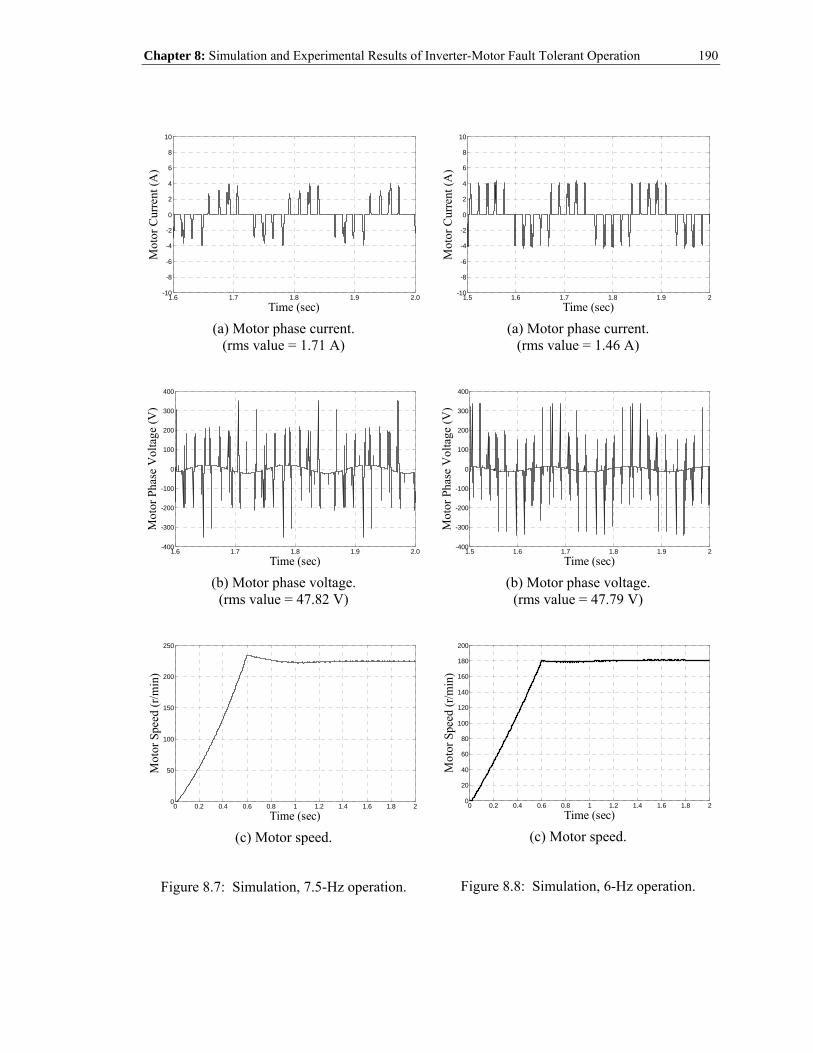
Chapter 8: Simulation and Experimental Results of Inverter-Motor Fault Tolerant Operation
190
1.6 1.7 1.8 1.9 2.0-10
-8
-6
-4
-2
0
2
4
6
8
10
Mot
or C
urre
nt (A
)
Time (sec) (a) Motor phase current.
(rms value = 1.71 A)
1.5 1.6 1.7 1.8 1.9 2-10
-8
-6
-4
-2
0
2
4
6
8
10
Mot
or C
urre
nt (A
)
Time (sec) (a) Motor phase current.
(rms value = 1.46 A)
1.6 1.7 1.8 1.9 2.0-400
-300
-200
-100
0
100
200
300
400
Mot
or P
hase
Vol
tage
(V)
Time (sec) (b) Motor phase voltage.
(rms value = 47.82 V)
1.5 1.6 1.7 1.8 1.9 2-400
-300
-200
-100
0
100
200
300
400
Mot
or P
hase
Vol
tage
(V)
Time (sec) (b) Motor phase voltage.
(rms value = 47.79 V)
0 0.2 0.4 0.6 0.8 1 1.2 1.4 1.6 1.8 20
50
100
150
200
250
Mot
or S
peed
(r/m
in)
Time (sec) (c) Motor speed.
Figure 8.7: Simulation, 7.5-Hz operation.
0 0.2 0.4 0.6 0.8 1 1.2 1.4 1.6 1.8 20
20
40
60
80
100
120
140
160
180
200
Mot
or S
peed
(r/m
in)
Time (sec) (c) Motor speed.
Figure 8.8: Simulation, 6-Hz operation.

Chapter 8: Simulation and Experimental Results of Inverter-Motor Fault Tolerant Operation
191
0.9 1 1.1 1.2 1.3 1.4 1.5-10
-8
-6
-4
-2
0
2
4
6
8
10
Mot
or C
urre
nts (
A)
Time (sec)
IaIbIc
(a)
0.9 1 1.1 1.2 1.3 1.4 1.5-10
-5
0
5
10
15
20
Dev
elop
ed T
orqu
e (N
m)
Time (sec) (b)
0.9 1 1.1 1.2 1.3 1.4 1.50
200
400
600
800
1000
1200
1400
1600
1800
Mot
or S
peed
(r/m
in)
Time (sec) (c)
Figure 8.9: Simulation results of motor performance at 60-Hz operation during pre- and post-fault conditions. (a) Three-phase currents. (b) Developed torque. (c) Motor speed.

Chapter 8: Simulation and Experimental Results of Inverter-Motor Fault Tolerant Operation
192
This dc (unidirectional) offset is divided between the paths of the remaining two healthy phases,
given that the motor has an isolated (floating) neutral connection. The electromagnetic interaction
between the stator current dc (unidirectional) component and the fundamental component of the
rotor magnetic field generates a pulsating torque at the stator line current frequency, as illustrated
from t = 1 sec to t = 1.3 sec in Figure 8.9(b), and the consequent corresponding speed ripples are
shown in Figure 8.9(c). Moreover, the dc (unidirectional) component of the stator current
generates unequal current stresses in the upper and lower transistor switches which may have
thermal consequences in these transistors and may need further consideration. As one may
observe from Figure 8.9(a), the phase currents revert to their healthy state when the SCRs are
commanded to turn-on at t = 1.3 sec to perform the bypass transfer in which the motor is now
being energized directly from the supply mains. Also, one can notice that there were no
significant interruptions during the point of bypass transfer in the motor phase currents, torque,
and speed profiles, owing to the fact that the inverter PWM reference (modulation) waveforms
are in synchronism with the supply mains through a PLL routine.
In order to demonstrate variable speed operations using the proposed discrete-frequency
control technique, the simulations were carried out under rated-load condition (8.169 Nm) at two
other frequencies, namely at 30-Hz and 15-Hz. The three-phase motor current waveforms during
pre- and post-fault operating conditions for the 30-Hz control are shown in Figure 8.10(a), and
the corresponding detail (zoom) of the steady-state “limp-home” post-fault current is shown in
Figure 8.10(b). It may appear from Figure 8.10(a) that the post-fault currents have increased by
more than twice their values of the healthy currents at rated-load condition. This is in fact not true
when the total rms value of the post-fault current of Figure 8.10(b) is computed and given, along
with the corresponding harmonic contents of the “limp-home” post-fault motor phase voltage and
current, in Table 8.2. From the harmonic contents, the total rms value of the current was
computed to be 4.261 Amps, which is about 1.42 times that of the rated case-study motor phase

Chapter 8: Simulation and Experimental Results of Inverter-Motor Fault Tolerant Operation
193
current which is 3 Amps (rms). Despite the need for the increased currents to obtain the desired
full-load torque, the amount of current increase is still less than that of the previous method
proposed by other researchers [49]-[51], which is 3 times that of the rated motor phase current.
In fact, the increased current value by a factor of 3 in the topology of [49]-[51] will result in a
motor neutral current of 3 times that of the rated motor phase current. Also, no motor neutral
connection is necessary for the presently conceived approach. Due to the non-sinusoidal nature of
the “limp-home” post-fault currents, torque pulsations and speed ripples will arise, as can be seen
from Figure 8.10(c) and Figure 8.10(d), respectively. Nevertheless, the torque pulsations are
significantly reduced, as compared to the faulty case, upon introducing the control algorithm of
the “limp-home” strategy. In addition, the motor is able to maintain the desired speed associated
with the 30-Hz frequency during the “limp-home” operation.
The same simulation was carried out for the case of 15-Hz frequency control at full-load
motor condition. The results are depicted in Figure 8.11 for the motor phase currents, developed
torque, and motor speed. Again, torque pulsations and speed ripples, as a result of the “limp-
home” operation, are evident from Figure 8.11(c) and Figure 8.11(d), respectively. The harmonic
contents of the motor phase voltage and current, along with their rms values, are given in Table
8.3. The total rms value of the motor phase current for the 15-Hz control operation was calculated
to be 4.392 Amps, which is about 1.464 times that of the rated rms current value (3 Amps rms) at
full-load condition. Again, this amount of increase in the motor phase current is still considerably
less than the necessary increase (1.73 times) required by the previously reported method of [49]-
[51] for full-load motor condition. Table 8.4 summarizes the torque pulsation in percent for both
the cases of the 30-Hz and the 15-Hz operations, during pre- and post-fault full-load conditions.
Due to the presence of torque and speed ripples, the present approach that may be acceptable for
“limp-home” purposes, such as in vehicles and other propulsion applications, fans, cement mills,
mine hoists, rolling mills and the like, is not suitable for applications such as paper mills or

Chapter 8: Simulation and Experimental Results of Inverter-Motor Fault Tolerant Operation
194
0.8 1 1.2 1.4 1.6 1.8 2-20
-15
-10
-5
0
5
10
15
20
Mot
or C
urre
nts (
A)
Time (sec)
IaIbIc
(a)
1.9 1.92 1.94 1.96 1.98 2-20
-15
-10
-5
0
5
10
15
20
Mot
or C
urre
nts (
A)
Time (sec)
(b) rms value = 4.261 A
0.8 1 1.2 1.4 1.6 1.8 2-10
-5
0
5
10
15
20
Dev
elop
ed T
orqu
e (N
m)
Time (sec) (c) Average torque = 8.169 Nm

Chapter 8: Simulation and Experimental Results of Inverter-Motor Fault Tolerant Operation
195
0.8 1 1.2 1.4 1.6 1.8 20
100
200
300
400
500
600
700
800
900
1000
Mot
or S
peed
(r/m
in)
Time (sec) (d) Average speed = 871 r/min
Figure 8.10: Simulation results of motor performance at 30-Hz operation during pre- and post-fault conditions at full-load. (a) Three-phase currents. (b) Steady-state “limp-home” post-fault
current. (c) Developed torque. (d) Motor speed.
Table 8.2: Simulation results of harmonic contents of motor phase voltage and current during post-fault limp-home at 30-Hz operation under full-load (8.169 Nm) condition.
Harmonic Order
Harmonic Frequency (Hz)
Motor Phase Voltage (rms value - Volts)
Motor Phase Current (rms value - Amps)
1 30 156.80 2.780 2 60 35.24 2.514 4 120 43.75 1.633 5 150 37.02 1.127 7 210 12.55 0.275 8 240 1.67 0.031
10 300 14.13 0.217 11 330 13.58 0.190 13 390 3.02 0.036 14 420 3.64 0.040 16 480 9.35 0.090 17 510 7.66 0.069 19 570 1.08 0.009 20 600 4.63 0.036
Total RMS Value: 173.19 4.261
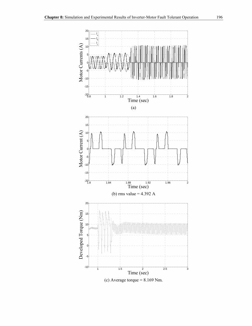
Chapter 8: Simulation and Experimental Results of Inverter-Motor Fault Tolerant Operation
196
0.8 1 1.2 1.4 1.6 1.8 2-20
-15
-10
-5
0
5
10
15
20
Mot
or C
urre
nts (
A)
Time (sec)
IaIbIc
(a)
1.8 1.84 1.88 1.92 1.96 2-20
-15
-10
-5
0
5
10
15
20
Mot
or C
urre
nt (A
)
Time (sec) (b) rms value = 4.392 A
1 1.5 2 2.5 3-10
-5
0
5
10
15
20
Dev
elop
ed T
orqu
e (N
m)
Time (sec) (c) Average torque = 8.169 Nm.

Chapter 8: Simulation and Experimental Results of Inverter-Motor Fault Tolerant Operation
197
1 1.5 2 2.5 30
50
100
150
200
250
300
350
400
450
500
Mot
or S
peed
(r/m
in)
Time (sec) (d) Average speed = 419 r/min
Figure 8.11: Simulation results of motor performance at 15-Hz operation during pre- and post-fault conditions at full-load. (a) Three-phase currents. (b) Steady-state “limp-home” post-fault
current. (c) Developed torque. (d) Motor speed.
Table 8.3: Simulation results of harmonic contents of motor phase voltage and current during post-fault limp-home at 15-Hz operation under full-load (8.169 Nm) condition.
Harmonic Order
Harmonic Frequency (Hz)
Motor Phase Voltage (rms value - Volts)
Motor Phase Current (rms value - Amps)
1 15 64.48 2.341 2 30 8.394 1.016 4 60 37.21 2.655 5 75 5.633 0.223 7 105 36.01 2.002 8 120 16.25 0.696
10 150 20.16 0.795 11 165 8.101 0.252 13 195 3.114 0.072 14 210 11.02 0.288 16 240 4.580 0.164 17 255 22.05 0.488 19 285 0.928 0.015 20 300 14.38 0.267
Total RMS Value: 94.54 4.392

Chapter 8: Simulation and Experimental Results of Inverter-Motor Fault Tolerant Operation
198
Table 8.4: Simulation results of torque pulsations during pre- and post-fault “limp-home” conditions at full-load (8.169 Nm).
Torque Ripple % of Average Torque Commanded Output
Frequency Pre-Fault During Fault Post-Fault Limp-Home
30-Hz 10.18 % 270.49 % 52.64 % 15-Hz 5.49 % 239.57 % 65.11 %
conveyor belt-driven types of applications where torque pulsation constitutes a major concern.
All things considered, the present approach is still able to maintain the desired motor speed
associated with the commanded output frequency during the post-fault “limp-home” operation.
8.2.2.3 Starting Performance of the Conceived Topology
An “upside” of the present topology is its ability to start-up with reduced starting currents
and minimum starting torque transients. With this feature, the present topology can function as a
drive with starting behavior that is comparable to that of a typical constant volts-per-hertz PWM
drive. This is carried out using the soft-starting algorithm that was presented in the earlier
chapters. The notion is to soft-start the motor before using the discrete-frequency control scheme
to control the motor to the desired speed that is associated with the commanded output frequency.
The starting performance of the present topology is demonstrated here for the case of 15-Hz and
12-Hz operations under half-load (4.084 Nm) and full-load (8.169 Nm) conditions.
The starting performance of the motor phase currents, developed torque, and motor speed for
the case of 15-Hz control under full-load (8.169 Nm) condition is shown in Figure 8.12(a)
through Figure 8.12(c), respectively. As one can observe from Figure 8.12(a), the motor
experiences reduced starting inrush currents during starting, which consequently result in reduced
starting torque pulsations, see Figure 8.12(b), and reduced speed ripples, see Figure 8.12(c). At
the time instant, t = 0.6 sec, the discrete-frequency control scheme which is initiated at that

Chapter 8: Simulation and Experimental Results of Inverter-Motor Fault Tolerant Operation
199
instant causes the motor to approach the desired speed at the commanded 15-Hz frequency. As
can be seen from the torque and speed profiles, there is a slight transient before the motor reaches
the desired speed. The same simulation was carried out at 15-Hz operation under half-load (4.084
Nm) condition. The results of the motor phase currents, developed torque, and motor speed are
depicted in Figure 8.13(a) through Figure 8.13(c), respectively. Again, one can see a similar trend
in the starting performance as compared to the full-load case, that is with reduced starting
currents and torque transients. A simulation was carried out at a different output frequency of 12-
Hz to demonstrate the starting behavior of the present conceived topology. The simulation results
of which are illustrated in Figure 8.14 and Figure 8.15 for the case of full-load and half-load
conditions, respectively. Conclusion similar to those mentioned above regarding the starting
performance of the present motor-inverter topology can be reached for these results shown in
Figure 8.14 and Figure 8.15. The steady-state motor performance, in terms of phase current rms
value, torque ripple %, and speed ripple %, of the results presented in Figure 8.12 through Figure
8.15 are summarized in Table 8.5.

Chapter 8: Simulation and Experimental Results of Inverter-Motor Fault Tolerant Operation
200
0 0.2 0.4 0.6 0.8 1 1.2 1.4 1.6 1.8 2-30
-20
-10
0
10
20
30
Mot
or C
urre
nt (A
)
Time (sec) (a) rms value = 4.392 A
0 0.2 0.4 0.6 0.8 1 1.2 1.4 1.6 1.8 20
5
10
15
20
25
Dev
elop
ed T
orqu
e (N
m)
Time (sec) (b) Average torque = 8.169 Nm
0 0.2 0.4 0.6 0.8 1 1.2 1.4 1.6 1.8 20
50
100
150
200
250
300
350
400
450
500
Mot
or S
peed
(r/m
in)
Time (sec) (c) Average speed = 418 r/min
Figure 8.12: Simulation results of soft-starting performance of present topology for 15-Hz operation at full-load (8.169 Nm) condition. (a) Motor phase current. (b) Torque. (c) Speed.

Chapter 8: Simulation and Experimental Results of Inverter-Motor Fault Tolerant Operation
201
0 0.2 0.4 0.6 0.8 1 1.2 1.4 1.6 1.8 2-30
-20
-10
0
10
20
30
Mot
or C
urre
nt (A
)
Time (sec) (a) rms value = 3.237 A
0 0.2 0.4 0.6 0.8 1 1.2 1.4 1.6 1.8 20
5
10
15
20
25
Dev
elop
ed T
orqu
e (N
m)
Time (sec) (b) Average torque = 4.084 Nm
0 0.2 0.4 0.6 0.8 1 1.2 1.4 1.6 1.8 20
50
100
150
200
250
300
350
400
450
500
Mot
or S
peed
(r/m
in)
Time (sec) (c) Average speed = 426 r/min
Figure 8.13: Simulation results of soft-starting performance of present topology for 15-Hz operation at half-load (4.084 Nm) condition. (a) Motor phase current. (b) Torque. (c) Speed.

Chapter 8: Simulation and Experimental Results of Inverter-Motor Fault Tolerant Operation
202
0 0.2 0.4 0.6 0.8 1 1.2 1.4 1.6 1.8 2-30
-20
-10
0
10
20
30
Mot
or C
urre
nts (
A)
Time (sec)
(a) rms value = 4.504 A
0 0.2 0.4 0.6 0.8 1 1.2 1.4 1.6 1.8 20
5
10
15
20
25
Dev
elop
ed T
orqu
e (N
m)
Time (sec) (b) Average torque = 8.169 Nm
0 0.2 0.4 0.6 0.8 1 1.2 1.4 1.6 1.8 20
50
100
150
200
250
300
350
400
Mot
or S
peed
(r/m
in)
Time (sec) (c) Average speed = 331 r/min
Figure 8.14: Simulation results of soft-starting performance of present topology for 12-Hz operation at full-load (8.169 Nm) condition. (a) Motor phase current. (b) Torque. (c) Speed.

Chapter 8: Simulation and Experimental Results of Inverter-Motor Fault Tolerant Operation
203
0 0.2 0.4 0.6 0.8 1 1.2 1.4 1.6 1.8 2-30
-20
-10
0
10
20
30
Mot
or C
urre
nt (A
)
Time (sec) (a) rms value = 3.339 A
0 0.2 0.4 0.6 0.8 1 1.2 1.4 1.6 1.8 20
5
10
15
20
25
Dev
elop
ed T
orqu
e (N
m)
Time (sec) (b) Average torque = 4.084 Nm
0 0.2 0.4 0.6 0.8 1 1.2 1.4 1.6 1.8 20
50
100
150
200
250
300
350
400
Mot
or S
peed
(r/m
in)
Time (sec) (c) Average speed = 340 r/min
Figure 8.15: Simulation results of soft-starting performance of present topology for 12-Hz operation at half-load (4.084 Nm) condition. (a) Motor phase current. (b) Torque. (c) Speed.

Chapter 8: Simulation and Experimental Results of Inverter-Motor Fault Tolerant Operation
204
Table 8.5: Simulation results of steady-state motor performance under full-load and half-load conditions for 15-Hz and 12-Hz motor operations.
Commanded Output
Frequency
Phase Current (rms - Amps)
Torque Ripple (% of Full-Load
Torque)
Speed Ripple (% of Average
Speed)
Full-Load (8.169 Nm) 15-Hz 4.392 A 65.11 % 1.34 %
12-Hz 4.504 A 70.14 % 2.33 %
Half-Load (4.084 Nm) 15-Hz 3.237 A 33.48 % 0.71 % 12-Hz 3.339 A 39.61 % 1.18 %
8.3 Experimental Validations
A hardware prototype of a PWM drive along with the conceived quasi-cycloconverter
power topology was built and tested in the laboratory, as depicted here in the circuit schematic of
Figure 8.16 and the photographs of Figure 8.17. The quasi-cycloconverter has the same power
configuration as the soft starter prototype that was utilized in the earlier experimental work as
reported in Chapter 5. For more details on the configurations and specifications of the quasi-
cycloconverter and the PWM drive, Appendix A should be consulted. Since the soft starter power
circuit topology consists of only three sets of back-to-back connected SCRs, two more sets of
similar SCRs are required for the conceived quasi-cycloconverter to operate at more selectable
frequencies/speeds, that is at o sf f N= , where N = 2, 5, 8, 11, 14, 17, 20, 23, 26, 29,…,
3k+2,…,etc. Here, k = 0, 1, 2, 3, 4,…,etc. Therefore, instead of adding two more sets of SCR
switches to the hardware prototype, two of the phases of the utility mains that are connected to
the SCR bridge are manually interchanged whenever the need to test the prototype at the
aforementioned commanded output frequency arises.

Chapter 8: Simulation and Experimental Results of Inverter-Motor Fault Tolerant Operation
205
a
b
cn
Indu
ctio
nM
otor
S 1S 3
S 5
S 4S
6S 2
ab
c
i ai b
i c
V sa V sb V sc
L fa
L fb L fc
Dio
deR
ectif
ier
Brid
geIn
verte
rBr
idge
Util
ityD
CLi
nkAC
Cho
ke D1
D3
D5
D4
D6
D2
15 k
W46
0 V
ac18
Am
ps60
Hz
4.8
%Z
Rsa
Rsb Rsc
L sa L sb L sc
0.70
81.
88 m
H
0.70
81.
88 m
H
0.70
81.
88 m
H
Con
tact
or
0.45
mH
0.45
mH
0.45
mH
Vac
Sens
or(S
ourc
e)
Vs a
GN
D
Vs b
Vsc
200
120
Vac
Switc
h
Onl
y us
ed1
out o
f 3-P
hase
R1 30 k
R2 30 k
Cdc
1
Cdc
2
2000
uF
2000
uF
TI D
SP &G
ate
Driv
e
Pre
char
geM
echa
nism
Vac
Sens
or(M
otor
)Vm
aV
mb
Vm
c
Iac
Sens
or(M
otor
)Im
aIm
bIm
c
A1
A 2co
il
Spec
ifica
tions
1. U
tility
: 15
kW, 4
60 V
ac, 1
8 A
mps
, 60
Hz,
4.8
%Z
2. C
onta
ctor
: 3-P
hase
, 120
Vac
coi
l, 90
Am
ps /
600
Vac
Max
Rat
ings
3. A
C C
hoke
Indu
ctor
: 3-P
hase
, 0.4
5 m
H /
35 A
mps
eac
h4.
Driv
e: 3
-Pha
se, 1
5 H
P, 4
40 -
500
Vac
, 21
Am
ps, 5
0/60
Hz
5. R
ectif
ier:
Sem
ikro
n, S
emip
ont,
SKD
82/
16, 3
-Pha
se, 8
0 A
mps
/ 16
00 V
6. D
C L
ink
Cap
acito
r: 2
@ 2
000
uF /
430
Vdc
each
7. In
vert
er: S
emik
ron,
Sem
itran
s, S
KM 7
5GB1
23D
, 1-L
eg, 7
5 A
mps
/ 12
00 V
8. G
ate
Driv
e: S
emik
ron,
Sem
idriv
er, S
KH
I 61,
6 P
WM
Out
puts
, On:
+15
V,
Off:
-6.5
V, 5
0 kH
z M
ax S
wFr
eq, +
15 V
dc S
uppl
y9.
Pre
char
ge M
echa
nsim
: 3-P
hase
Con
tact
or, 1
20 V
ac c
oil,
25 A
/ 60
0 Va
c
M
ax R
atin
gs, R
esis
tor (
Ohm
ite, L
225J
100E
) = 1
00 o
hms
@ 2
25 W
atts
(2 in
ser
ies)
10. F
an: 2
4 Vd
c, 0
.28
Amps
, 6.7
Wat
ts, R
ed+
Blac
k-11
. Mot
or: 2
HP,
4-P
ole,
230
/460
Vac
, 6.0
/3.0
Am
ps, 1
744
rpm
, 60
Hz
12. S
CR
Brid
ge: S
emik
ron,
Sem
itop
3, S
K 4
5 U
T 16
, 3-P
hase
, 47
A / 1
600
V13
. Snu
bber
: R =
57
ohm
s (5
%),
C =
112
pF
(20%
) (M
odel
: X5F
, 3 k
V ra
ting)
14. D
SP C
ontr
olle
r: Te
xas
Inst
rum
ents
, TM
S32
0F28
12, F
ixed
-Poi
nt D
SP15
. Sen
sor:
LEM
, Cur
rent
Tra
nsdu
cer L
F 30
5-S
, 300
Am
ps (r
ms)
16. S
igna
l Con
ditio
ning
: Pul
se T
rans
form
ers
+ A
nalo
g C
ircui
ts17
. Dat
a A
cqui
sitio
n: N
atio
nal I
nstru
men
ts, P
CI-6
052E
, 333
kSa
mpl
es/s
ec
SKD
82/
16SK
M 7
5GB1
23D
SK 4
5 U
T 16
SC
R B
ridge
5711
2pF Gat
eP
ulse
s
Sign
alC
ondi
tioni
ngC
ircui
ts
DSP
Con
trol
ler
Volta
ge &
Cur
rent
Feed
back
sD
AQ
Syst
em
Figure 8.16: Schematic and specifications of induction motor-drive test setup system.

Chapter 8: Simulation and Experimental Results of Inverter-Motor Fault Tolerant Operation
206
(a)
2-hp Induction Motor
Dyne
Dyne Controller
(b)
Figure 8.17: Test rigs. (a) PWM drive and quasi-cycloconverter power topology. (b) Induction motor and dynamometer.
SCR Bridges
Current Sensors
Pulse Transformers
+ Signal
Conditioning Boards
TI DSP Board
PWM Drive
Gate Drive

Chapter 8: Simulation and Experimental Results of Inverter-Motor Fault Tolerant Operation
207
8.3.1 The No-Load Case
Experimental results of steady-state motor performance at no-load condition obtained from
using the conceived quasi-cycloconverter power circuit topology for the different cases of
commanded output frequencies, that is at f = 30-Hz, 15-Hz, 12-Hz, 8.57-Hz, 7.5-Hz, and 6-Hz,
are presented first. These test results at the aforementioned frequencies are depicted in Figure
8.18 through Figure 8.23, respectively. As one may observe from these test figures, the measured
current waveforms match reasonably well with the simulation current waveforms given in Figure
8.3(a) through Figure 8.8(a), in so far as the profiles are concerned. The same observation can be
made for the measured waveforms of the motor phase voltages shown in Figure 8.18(b) through
Figure 8.23(b), in comparison with the simulation phase voltage waveforms given in Figure
8.3(b) through Figure 8.8(b), for the different commanded output frequencies. Notice from the
voltage waveforms the presence of a low-frequency harmonic component which corresponds to
the commanded output frequency. Hence, the experimental results presented herein clearly verify
the soundness of the theory of the conceived discrete-frequency control algorithm being applied
using the conceived quasi-cycloconverter power circuit topology.
8.3.2 Limp-Home Operation of the Conceived Topology under
Inverter Fault Case
The test results of the motor performance under inverter switch fault case are first presented.
The measured three-phase current waveforms at 15-Hz output frequency and 25% load condition
(~ 2 Nm), in the event of a transistor open-circuit switch fault at S1, are depicted in Figure 8.24.
These current waveforms are in good agreement with the simulation waveforms, as depicted in
Figure 6.14(b) of Chapter 6, in so far as the profiles are concerned. In order to further investigate
the motor performance due to an open-circuit switch fault, the current space-vector locus,
obtained by plotting the measured waveforms of id versus iq current components, under different

Chapter 8: Simulation and Experimental Results of Inverter-Motor Fault Tolerant Operation
208
Mot
or C
urre
nt (5
A/d
iv)
Time (20 ms/div) (a) Motor phase current.
(rms value = 1.48 A)
Mot
or P
hase
Vol
tage
(200
V/d
iv)
Time (20 ms/div) (b) Motor phase voltage.
(rms value = 81.54 V)
Figure 8.18: Experimental results, 30-Hz operation.
Mot
or C
urre
nt (5
A/d
iv)
Time (40 ms/div) (a) Motor phase current.
(rms value = 1.30 A)
Mot
or P
hase
Vol
tage
(200
V/d
iv)
Time (40 ms/div) (b) Motor phase voltage.
(rms value = 52.64 V)
Figure 8.19: Experimental results, 15-Hz operation.
Mot
or C
urre
nt (5
A/d
iv)
Time (50 ms/div) (a) Motor phase current. (rms value = 0.948 A)
Mot
or P
hase
Vol
tage
(200
V/d
iv)
Time (50 ms/div) (b) Motor phase voltage.
(rms value = 49.33 V)
Figure 8.20: Experimental results, 12-Hz operation.

Chapter 8: Simulation and Experimental Results of Inverter-Motor Fault Tolerant Operation
209
Mot
or C
urre
nt (5
A/d
iv)
Time (100 ms/div) (a) Motor phase current.
(rms value = 1.14 A)
Mot
or P
hase
Vol
tage
(200
V/d
iv)
Time (100 ms/div) (b) Motor phase voltage.
(rms value = 47.47 V)
Figure 8.21: Experimental results, 8.57-Hz operation.
Mot
or C
urre
nt (5
A/d
iv)
Time (100 ms/div) (a) Motor phase current. (rms value = 0.673 A)
Mot
or P
hase
Vol
tage
(200
V/d
iv)
Time (100 ms/div) (b) Motor phase voltage.
(rms value = 35.99 V)
Figure 8.22: Experimental results, 7.5-Hz operation.
Mot
or C
urre
nt (5
A/d
iv)
Time (100 ms/div) (a) Motor phase current.
(rms value = 1.05 A)
Mot
or P
hase
Vol
tage
(200
V/d
iv)
Time (100 ms/div) (b) Motor phase voltage.
(rms value = 42.87 V)
Figure 8.23: Experimental results, 6-Hz operation.

Chapter 8: Simulation and Experimental Results of Inverter-Motor Fault Tolerant Operation
210
Mot
or C
urre
nts (
5 A
/div
)
Time (40 ms/div)
IaIbIc
Figure 8.24: Measured three-phase motor current waveforms at 15-Hz output frequency, 25% load condition under an inverter open-circuit switch fault at S1.
locations of the faulty transistor switch are plotted and shown here, along with the healthy case,
under the condition of 15-Hz output frequency and 25% load, in Figure 8.25. Again, these current
space-vector loci match reasonably well with those obtained from the simulation results, as given
earlier in Figure 6.20 of Chapter 6.
In order to experimentally validate / verify the “limp-home” motor performance using the
conceived approach, the experimental work was carried out at 15-Hz output frequency under 25%
load (~ 2 Nm) condition. The test was first run in the healthy PWM drive condition, and
thereafter an open-circuit switch fault was deliberately introduced at switch, S1. After one second
from which the fault had occurred, the “limp-home” strategy was initiated. The test result of the
three-phase motor current waveforms demonstrating pre-fault, during fault, and post-fault cases is
depicted in Figure 8.26. As one may observe from Figure 8.26, the seamless transition from one
case to another is in considerably good agreement with the simulation waveforms in profiles,
given in Figure 8.11(a), for the case of 15-Hz output frequency. The differences in the rms
current magnitudes of the simulation and test results during pre-fault and post-fault conditions are

Chapter 8: Simulation and Experimental Results of Inverter-Motor Fault Tolerant Operation
211
(a) Healthy.
(b) Open-circuit fault at S1.
(c) Open-circuit fault at S4.
(d) Open-circuit fault at S3.
(e) Open-circuit fault at S6.
(f) Open-circuit fault at S5.
(g) Open-circuit fault at S2.
Figure 8.25: Experimental results of current space-vector locus at 15-Hz, 25% load condition.

Chapter 8: Simulation and Experimental Results of Inverter-Motor Fault Tolerant Operation
212
Mot
or C
urre
nts (
5 A
/div
)
Time (500 ms/div)
IaIbIc
Healthy PWM Drive Operation Open-Circuit Fault at S1 Limp-Home Operation
rms = 1.936Arms = 1.415A
Figure 8.26: “Limp-home” motor performance of measured phase currents at 15-Hz, 25% load condition in the event of an inverter open-circuit switch fault at S1.
due to the fact that the simulation was carried out under full-load condition, whereas the test was
carried out at 25% load condition.
The test results of the steady-state post-fault motor performance using the conceived “limp-
home” strategy under motor loading conditions at full-load and half-load for the case of 15-Hz (N
= 4) and 12-Hz (N = 5) motor operations are presented next. For the case of 12-Hz motor
operation, two phases of the supply mains are manually interchanged in the test setup in order to
impress negative-sequence voltages at the input terminals of the SCR bridge. The purpose of this
interchange is to ensure that the sequence of the fundamental components of the voltages received
at the motor terminals from the output of the SCR bridge shall always possess a positive-
sequence to produce the same forward rotation of the motor, as a result of using the present
control scheme. The measured waveforms of the motor phase current, voltage, and developed
torque for the full-load and half-load conditions are given here in Figure 8.27(a)-(c) and Figure
8.28(a)-(c), respectively. Notice that the developed (airgap) torque illustrated here was acquired
implicitly from the measured motor terminal quantities (currents and voltages) using the
expression in (5.2) given in Chapter 5 of this dissertation [95]. The measured current waveforms

Chapter 8: Simulation and Experimental Results of Inverter-Motor Fault Tolerant Operation
213
of Figure 8.27(a) and Figure 8.28(a) have similar shapes to the steady-state portion of the
simulation phase current waveforms given earlier in Figure 8.12(a) and Figure 8.13(a), which are
repeated here in “zoom” form in Figure 8.29(a) and Figure 8.30(a), for the full-load and half-load
cases, respectively. Due to the non-sinusoidal nature of the current waveforms, torque ripple
contents are clearly evident from the developed (airgap) torque computed from the experimental
readings of the motor terminal operating conditions, which are shown in Figure 8.27(c) and
Figure 8.28(c) for the different load cases. The “zoom” forms of the corresponding simulation
torque profiles, given earlier in Figure 8.12(b) and Figure 8.13(b), are repeated here in Figure
8.29(b) and Figure 8.30(b), respectively, for comparison purposes.
To further demonstrate the performance of the motor using the conceived topology and
control strategy, the experimental work was carried out at the commanded output frequency of
12-Hz, the results of which are depicted in Figure 8.31 and Figure 8.32 under full-load and half-
load conditions, respectively. Again, the test results match considerably well with the steady-state
portions of the simulation waveforms of the motor phase currents and developed torques shown
in Figure 8.14(a)-(b) and Figure 8.15(a)-(b), with their corresponding “zoom” forms given in
Figure 8.33(a)-(b) and Figure 8.34(a)-(b), under full-load and half-load conditions, respectively.
The motor performance in terms of torque ripple (%) and total rms current values for both the
simulation and experimental results for the case of the 15-Hz and 12-Hz motor operations under
full-load and half-load conditions are summarized in Table 8.6. It can be seen from this table that
the simulation results are in fairly good agreement with the experimental test results. Even though
the torque ripples are considerably higher at full-load condition, these torque ripples are reduced
by about one-half under half-load condition. Furthermore, the motor rms phase currents are also
reduced to near their rated value at half-load condition. Hence, this implies that the present
approach is most suitable for light motor-load applications. Practical application considerations
and opportunities for use of the present design will be further detailed in the forthcoming section.

Chapter 8: Simulation and Experimental Results of Inverter-Motor Fault Tolerant Operation
214
Mot
or C
urre
nt (5
A/d
iv)
Time (40 ms/div) (a) rms value = 4.297 A
Mot
or P
hase
Vol
tage
(200
V/d
iv)
Time (40 ms/div) (b) rms value = 90.99 V
0
Dev
elop
ed T
orqu
e (5
Nm
/div
)
Time (200 ms/div) (c) Average torque = 8.099 Nm
Figure 8.27: Experimental results of post-fault limp-home motor performance for 15-Hz operation at full-load condition. (a) Motor phase current. (b) Motor phase voltage. (c) Motor
developed torque.

Chapter 8: Simulation and Experimental Results of Inverter-Motor Fault Tolerant Operation
215
Mot
or C
urre
nt (5
A/d
iv)
Time (40 ms/div) (a) rms value = 2.934 A
Mot
or P
hase
Vol
tage
(200
V/d
iv)
Time (40 ms/div) (b) rms value = 75.11 V
0
Dev
elop
ed T
orqu
e (5
Nm
/div
)
Time (200 ms/div) (c) Average torque = 4.101 Nm
Figure 8.28: Experimental results of post-fault limp-home motor performance for 15-Hz operation at half-load condition. (a) Motor phase current. (b) Motor phase voltage. (c) Motor
developed torque.

Chapter 8: Simulation and Experimental Results of Inverter-Motor Fault Tolerant Operation
216
1.7 1.74 1.78 1.82 1.86 1.9-15
-10
-5
0
5
10
15
Mot
or C
urre
nt (A
)
Time (sec) (a) rms value = 4.392 A
1 1.2 1.4 1.6 1.8 20
5
10
15
20
25
Dev
elop
ed T
orqu
e (N
m)
Time (sec) (b) Average torque = 8.169 Nm
Figure 8.29: Steady-state “zoom” form of the simulation results of Figure 8.12 for 15-Hz operation at full-load (8.169 Nm) condition. (a) Motor phase current. (b) Torque.

Chapter 8: Simulation and Experimental Results of Inverter-Motor Fault Tolerant Operation
217
1.7 1.74 1.78 1.82 1.86 1.9-15
-10
-5
0
5
10
15
Mot
or C
urre
nt (A
)
Time (sec) (a) rms value = 3.237 A
1 1.2 1.4 1.6 1.8 20
5
10
15
20
25
Dev
elop
ed T
orqu
e (N
m)
Time (sec) (b) Average torque = 4.084 Nm
Figure 8.30: Steady-state “zoom” form of the simulation results of Figure 8.13 for 15-Hz operation at half-load (4.084 Nm) condition. (a) Motor phase current. (b) Torque.

Chapter 8: Simulation and Experimental Results of Inverter-Motor Fault Tolerant Operation
218
Mot
or C
urre
nt (5
A/d
iv)
Time (50 ms/div) (a) rms value = 4.317 A
Mot
or P
hase
Vol
tage
(200
V/d
iv)
Time (50 ms/div) (b) rms value = 101.04 V
0
Dev
elop
ed T
orqu
e (5
Nm
/div
)
Time (200 ms/div) (c) Average torque = 8.211 Nm
Figure 8.31: Experimental results of post-fault limp-home motor performance for 12-Hz operation at full-load condition. (a) Motor phase current. (b) Motor phase voltage. (c) Motor
developed torque.

Chapter 8: Simulation and Experimental Results of Inverter-Motor Fault Tolerant Operation
219
Mot
or C
urre
nt (5
A/d
iv)
Time (50 ms/div) (a) rms value = 3.032 A
Mot
or P
hase
Vol
tage
(200
V/d
iv)
Time (50 ms/div) (b) rms value = 76.73 V
0
Dev
elop
ed T
orqu
e (5
Nm
/div
)
Time (200 ms/div) (c) Average torque = 4.054 Nm
Figure 8.32: Experimental results of post-fault limp-home motor performance for 12-Hz operation at half-load condition. (a) Motor phase current. (b) Motor phase voltage. (c) Motor
developed torque.

Chapter 8: Simulation and Experimental Results of Inverter-Motor Fault Tolerant Operation
220
1.7 1.75 1.8 1.85 1.9 1.95 2-15
-10
-5
0
5
10
15
Mot
or C
urre
nt (A
)
Time (sec) (a) rms value = 4.504 A
1 1.2 1.4 1.6 1.8 20
5
10
15
20
25
Dev
elop
ed T
orqu
e (N
m)
Time (sec) (b) Average torque = 8.169 Nm
Figure 8.33: Steady-state “zoom” form of the simulation results of Figure 8.14 for 12-Hz operation at full-load (8.169 Nm) condition. (a) Motor phase current. (b) Torque.

Chapter 8: Simulation and Experimental Results of Inverter-Motor Fault Tolerant Operation
221
1.7 1.75 1.8 1.85 1.9 1.95 2-15
-10
-5
0
5
10
15
Mot
or C
urre
nt (A
)
Time (sec) (a) rms value = 3.339 A
1 1.2 1.4 1.6 1.8 20
5
10
15
20
25
Dev
elop
ed T
orqu
e (N
m)
Time (sec) (b) Average torque = 4.084 Nm
Figure 8.34: Steady-state “zoom” form of the simulation results of Figure 8.15 for 12-Hz operation at half-load (4.084 Nm) condition. (a) Motor phase current. (b) Torque.

Chapter 8: Simulation and Experimental Results of Inverter-Motor Fault Tolerant Operation
222
Table 8.6: Comparisons between simulation and experimental results for the case of 15-Hz and 12-Hz motor operations.
Simulation Experiment Current (rms) Torque Ripple Current (rms) Torque Ripple Commanded
Output Frequency (Amps) (% of Full-Load
Torque) (Amps) (% of Full-Load Torque)
Full-Load 15-Hz 4.392 65.11 % 4.297 64.49 % 12-Hz 4.504 70.14 % 4.317 73.11 %
Half-Load 15-Hz 3.237 33.48 % 2.934 30.90 % 12-Hz 3.339 39.61 % 3.032 36.29 %
8.3.3 Starting Performance of the Conceived Topology
The starting performance of the motor from standstill when using the conceived topology
was also verified / validated experimentally. The test results of the starting transient of the motor
phase current and the motor developed torque are presented in Figure 8.35(a) and (b),
respectively, for the case of 15-Hz operation at 25% load (~ 2 Nm) condition. The motor was first
energized using the open-loop symmetrical-triggering soft-starting control, before being driven
using the conceived discrete-frequency control scheme to achieve the desired speed that
corresponds to the commanded output frequency. As one can observe from Figure 8.35(a), the
motor experiences reduced starting inrush currents during starting, which consequently result in
reduced starting torque pulsations, see Figure 8.35(b). Also, one can notice from the torque
profile that there is a slight transient before the motor reaches the steady-state condition. It is
evident from the experimental results that the conceived topology clearly demonstrates smooth
starting performance, which in a sense emulates the starting behavior of a PWM drive which
utilizes volts per hertz control.

Chapter 8: Simulation and Experimental Results of Inverter-Motor Fault Tolerant Operation
223
Mot
or C
urre
nt (5
A/d
iv)
Time (500 ms/div) (a)
0
Dev
elop
ed T
orqu
e (2
Nm
/div
)
Time (500 ms/div) (b)
Figure 8.35: Experimental results of soft-starting performance of present topology for 15-Hz operation at 25% load (~ 2 Nm) condition. (a) Motor phase current. (b) Motor developed torque.
Chapter 8: Simulation and Experimental Results of Inverter-Motor Fault Tolerant Operation
224
8.4 Application Considerations and Opportunities
In many industrial applications, the average load factor of electric motors is estimated to be
less than 60% [101], [103]. In other words, these electric motors only operate up to 60% of their
rated conditions. In fact, in some industrial applications, the average load factor can be as low as
25% [103]. This means that the motor selected for any specific application is usually oversized.
Meanwhile, there are numerous applications in which low-speed operations are required, such as
vehicle and ship propulsion systems, cement mills, mine hoists, rolling mills and the like. Based
on these low-speed applications and the fact that oversized motors are usually selected according
to industrial standard, the present conceived approach is a good candidate for these types of low-
speed applications at partial motor-loading conditions. This is due to the fact that the present
approach, which is designed for low-speed operations, exhibits moderately low torque
ripples/pulsations at partial motor-loading conditions which makes it a perfect fit for “limp-
home” operations in such types of applications. Evidence supporting this claim is presented in the
following analysis.
An investigation was performed to study the nature of the torque ripple/pulsation resulting
from the conceived approach with regard to the motor frequency and the effect of the load torque
level. The motor torque ripple in percentage representation of the full-load motor torque was
obtained through simulation that was carried out under different output motor frequencies at
different load levels, the results of which are depicted in Figure 8.36. Examination of Figure 8.36
clearly shows that the torque ripple is dramatically reduced with decreasing load level. In
applications where a load factor of only 25% is required [103], the torque pulsation resulting from
this study can be seen to be less than 25% of the full-load torque, which may be tolerable for
“limp-home” operation for a certain period of time. One can also notice from the figure that the
torque pulsation increases as the motor output frequency decreases. This is due to the fact that the

Chapter 8: Simulation and Experimental Results of Inverter-Motor Fault Tolerant Operation
225
0 0.25 0.5 0.75 1 1.250
10
20
30
40
50
60
70
80
90
100
Torq
ue R
ippl
e (%
)
Load Torque (p.u.)
30-Hz15-Hz12-Hz8.57-Hz7.5-Hz6-Hz
Figure 8.36: Simulation results of torque-ripple percentage of full-load torque at different load levels.
motor’s moment of inertia, which behaves as a low-pass filter, filters out the higher-order torque
harmonics. This reduction of higher-order torque harmonics is extremely evident when the motor
is operating at a higher frequency. Similar study with regard to motor torque ripple/pulsation
calculation was also carried out using the experimental test results that were presented earlier.
The torque ripple/pulsation calculation from the test results, along with those from the
corresponding simulation results acquired from Figure 8.36, for the cases of 30-Hz, 15-Hz, and
12-Hz motor operations are illustrated in Figure 8.37. It is evident that one can see a considerably
good agreement between the computed torque ripple/pulsation in percentage between the
experimental test and simulation data.
Meanwhile, the rms phase currents of the test and simulation results under the foregoing
conditions were plotted in Figure 8.38 in per-unit representation of its rated value as a function of
the load torque. From Figure 8.38, one can see a reasonable degree of agreement in the rms phase
current values between the test and simulation results. Further examination of Figure 8.38 also

Chapter 8: Simulation and Experimental Results of Inverter-Motor Fault Tolerant Operation
226
indicates that the rms phase currents of the motor are within or below its rated current value when
the motor is operating at less than 50% of its rated condition. Therefore, thermal issues are not of
a major concern when the motor is operating at low-load condition using the conceived approach.
Hence, the curves presented in Figure 8.36 through Figure 8.38 support the earlier claim in which
it is safe to operate the motor at low-load conditions using the present conceived torque-speed
control approach with acceptable motor performance for reasonably limited periods of “limp-
home” operating time.
It has been reported earlier in [104]-[107] that it is a well-known fact that induction
machines could exhibit a region of instability when supplied by an adjustable-speed PWM drive.
The range of unstable operating frequencies is typically between 10-Hz and 35-Hz for a 6o-Hz
rated frequency, and the size and range of this unstable region is dependent upon the variation of
motor parameters under operating conditions, motor inertia, switching dead-time, PWM carrier
frequency, rectifier-inverter link parameter variations, and the load [104]-[107]. This instability
was observed during low-frequency motor-drive operation, and translates itself into undesirable
oscillations in the motor phase currents, which leads to an oscillating torque. Therefore, it appears
that the present conceived control approach could provide a better “limp-home” solution than
previously reported methods proposed by other researchers [38]-[59], when low-speed operation
constitutes the main concern. In addition, the present approach does not suffer from drawbacks
such as the need for accessibility to a motor neutral, larger size dc link capacitors, or higher dc
bus voltage. Another “upside” element of the conceived approach is its potential use for
mitigating other drive-related faults that can potentially occur in the diode-rectifier bridge or the
dc-link of the drive because of the fact that this approach bypasses the entire drive system, which
is not possible with the previous methods given in [38]-[59]. Therefore, the conceived approach
presents itself as a low-cost solution for prolonging the life of the motor-drive system in the event
of a fault in the drive, allowing the motor to function under limited torque-speed control means.

Chapter 8: Simulation and Experimental Results of Inverter-Motor Fault Tolerant Operation
227
0 0.25 0.5 0.75 1 1.250
10
20
30
40
50
60
70
80
90
100
Torq
ue R
ippl
e (%
)
Load Torque (p.u.)
30-Hz Motor Operation
SimulationExperiment
(a)
0 0.25 0.5 0.75 1 1.250
10
20
30
40
50
60
70
80
90
100
Torq
ue R
ippl
e (%
)
Load Torque (p.u.)
15-Hz Motor Operation
SimulationExperiment
(b)
0 0.25 0.5 0.75 1 1.250
10
20
30
40
50
60
70
80
90
100
Torq
ue R
ippl
e (%
)
Load Torque (p.u.)
12-Hz Motor Operation
SimulationExperiment
(c)
Figure 8.37: Torque-ripple percentage of full-load torque versus load torque at different output motor frequencies. (a) 30-Hz operation. (b) 15-Hz operation. (c) 12-Hz operation.
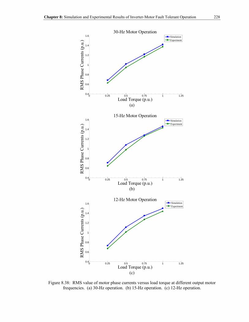
Chapter 8: Simulation and Experimental Results of Inverter-Motor Fault Tolerant Operation
228
0 0.25 0.5 0.75 1 1.250.4
0.6
0.8
1
1.2
1.4
1.6
RM
S Ph
ase
Cur
rent
s (p.
u.)
Load Torque (p.u.)
30-Hz Motor Operation
SimulationExperiment
(a)
0 0.25 0.5 0.75 1 1.250.4
0.6
0.8
1
1.2
1.4
1.6
RM
S Ph
ase
Cur
rent
s (p.
u.)
Load Torque (p.u.)
15-Hz Motor Operation
SimulationExperiment
(b)
0 0.25 0.5 0.75 1 1.250.4
0.6
0.8
1
1.2
1.4
1.6
RM
S Ph
ase
Cur
rent
s (p.
u.)
Load Torque (p.u.)
12-Hz Motor Operation
SimulationExperiment
(c)
Figure 8.38: RMS value of motor phase currents versus load torque at different output motor frequencies. (a) 30-Hz operation. (b) 15-Hz operation. (c) 12-Hz operation.

Chapter 8: Simulation and Experimental Results of Inverter-Motor Fault Tolerant Operation
229
8.5 Summary
In this chapter, the simulation and experimental test results of the conceived quasi-
cycloconverter-based “limp-home” strategy under inverter switch faults have been presented. The
presented simulation and test results have demonstrated the soundness and validity of the
conceived approach for practical use. Practical application considerations and opportunities for
use of the conceived design were also investigated. The results of the study suggest that the
conceived approach is best suited for partial motor-loading operating conditions, which is
normally the case for many practical industrial applications in which the motors are usually
oversized. Accordingly, this investigator perceives that there is still a place in real practice for the
present topology to “stand out” as a potential means of mitigating any drive-related faults, based
on its low-cost requirements as well as other merits that were previously mentioned and discussed
above.
230
CHAPTER 9
9 CONCLUSIONS, CONTRIBUTIONS, AND
SUGGESTED FUTURE WORK
9.1 Summary and Conclusions
In this chapter, the summary of the accomplishments of this work and main contributions of
this dissertation are reviewed. This is followed by recommendations and suggestions regarding
possible directions of future research topics.
In Chapter 1, the background and motivation of this work have been described with
emphasis on the importance of incorporating fault tolerant or “limp-home” capability for
prolonging/extending the life of an ac motor-drive system. A literature survey of the previous
research work performed by other investigators has been presented. Based on a simple
functionality categorization of the “limp-home” strategies of three-phase ac motor-drive systems,
some of the strategies have been briefly reviewed for some of the categories, with greater
emphasis on strategies that have been applied on the standard three-phase, six-switch inverter
type of adjustable-speed PWM drives. Such type of drives is the focal research element in this
work. Through this survey, it has been shown that the existing “limp-home” methods have their
own merits and drawbacks. The merits are the ability to maintain rated motor performance, while

Chapter 9: Conclusions, Contributions, and Suggested Future Work 231
the drawbacks are the essential system cost increase for maintaining continuous motor operation
in the event of an inverter switch fault. Also, these methods are only applicable for mitigating
inverter-type switch fault. To the knowledge of this investigator, no prior work has been done on
both the investigation of the effect of SCR switch fault of soft starters on motor performance and
the development of their corresponding remedial strategies during the occurrence of such fault.
Hence, this opens a door to this investigator to pursue his research area in the development of
low-cost fault-tolerant solutions for both the soft starters and adjustable-speed PWM drives. This
chapter is then concluded with the main objectives and contributions that this work brings about,
followed by the organization of this dissertation.
In Chapter 2, an analytical closed-form solution describing the transient performance of a
motor-soft starter system under healthy and faulty conditions has been presented. The types of
faults under study are the SCR open-circuit and short-circuit switch faults occurring only in one
phase of the soft starter system. Analytical closed-form expressions for the non-sinusoidal phase
voltages impressed upon the motor windings under both healthy and faulty soft starter operating
conditions have been derived. According to these closed-form voltage expressions, the well-
known T-equivalent circuit motor model was utilized to obtain the motor phase currents for the
fundamental voltage term and each subsequent harmonic voltage term. Superposition was then
applied to express the resulting motor phase currents in a Fourier series form. The closed-form
analytical studies demonstrate that the short-circuit SCR fault produces undesired fault response
on motor performance with unbalanced, high starting currents which accordingly result in high
starting torque pulsations. On the contrary, it is shown here that the open-circuit SCR switch fault
results in no starting torque from the motor. Hence it constitutes a total failure of motor starting.
On the other hand, it does not expose the soft starter elements to the severity of motor current
unbalances and the severity of motor torque pulsations. Evidently, the use of the conventional
open-loop symmetrical-triggering control in a two-phase switching mode under faulty condition

Chapter 9: Conclusions, Contributions, and Suggested Future Work 232
contribute to detrimental impacts on motor performance which result in disruption of normal
operation of the motor-load system during soft starting. With a better understanding of these fault
impacts, a remedial strategy was then developed to minimize the negative effects resulting from
such faults during normal soft starting operation.
In Chapter 3, the above mentioned remedial strategy consisting of a simple low-cost fault
tolerant solution capable of mitigating SCR open-circuit and short-circuit switch faults for soft
starters has been presented. Minimum hardware modifications are required for the existing
commercially available soft starter in order for the fault tolerant operation to be possible. It
should be emphasized that such essential modifications do not significantly increase the cost and
size of the existing system. One of the essential changes involves adding a set of three-phase
voltage transducers on the motor end of the soft starter for acquiring the motor terminal voltages
needed for fault tolerant control purposes. The second hardware modification involves the
replacement of the existing 3-pole synchronously-controlled modular bypass contactor with a set
of individually-controlled 1-pole contactors for all three phases. These contactors are used for
fault isolation purposes in such a way that the soft starter can switch into a two-phase switching
mode in the event of an SCR switch fault occurring in any one of the phases. As for the conceived
two-phase control approach, two types of feedback control loops were adopted and utilized
concurrently. Namely, these are the voltage and current feedback loops, respectively. The voltage
feedback control is responsible for the starting acceleration of the motor, while the current
feedback loop is responsible for mitigating the unbalanced effects of the starting currents under
thyristor switch fault condition. In fact, by adopting the proposed control technique, a low-cost
soft starter with only two-phase switching mode can be developed and produced in the market for
consumers at a lower cost with reasonably good performance, as compared to the existing three-
phase soft starter products.

Chapter 9: Conclusions, Contributions, and Suggested Future Work 233
In addition, small-signal modeling of the motor-soft starter controller system was developed.
More specifically, the open-loop and closed-loop transfer functions of the voltage and current
control feedback loop systems were derived. The main thrust of this small-signal modeling
approach was to design the PI regulators in the voltage and current loops so as to achieve the
desired bandwidth to render a good dynamic and fast transient response. Upon designing the PI
controllers, the entire system was simulated under large-signal conditions to evaluate the stability
and response of the controllers.
In Chapter 4, the accuracy of the closed-form analytical results from Chapter 2 was verified
versus the corresponding simulation results. It has been shown that the analytical results are in
good correlation with the simulation results, which raises confidence in the fidelity and value of
the analytical approach. Such efforts provide an alternative means of analyzing the transient
performance of the motor in lieu of using the elaborate simulation approach. In the same chapter,
the motor performance under three different control cases, namely, three-phase open-loop, two-
phase open-loop, and the newly conceived method with two-phase closed-loop controls were
simulated and compared. The newly conceived fault tolerant method with resilient control has
demonstrated reduced starting inrush currents, and consequently reduced starting torque
pulsations under SCR fault in one phase of the soft starter, as compared to the two-phase open-
loop control case. These promising results demonstrate the feasibility of the conceived strategy
for improving the reliability of an industrial-type three-phase soft starter system at a modest cost
increase.
In Chapter 5, the measured results during the soft starting transients under healthy and short-
circuit switch fault conditions were compared with the analytical and simulation results presented
earlier in Chapters 2 and 4, respectively. The objective was to verify the accuracy of the
analytical and detailed simulation work that was carried out earlier in Chapters 2 and 4,
respectively. The resulting comparisons indicate good agreements between the test, simulation,

Chapter 9: Conclusions, Contributions, and Suggested Future Work 234
and analytical waveforms. In the same chapter, the motor performance obtained from both the
experiment and simulation, under 3-phase open-loop, 2-phase open-loop, as well as the newly
conceived 2-phase closed-loop controls were compared. Overall, the experimental test results
match reasonably well with the simulation results. It is evident from both the test and simulation
results given in this and earlier chapters that the present newly conceived fault tolerant soft starter
has demonstrated its efficacy and practicability to be retrofitted into industrial-type three-phase
soft starter systems.
In Chapter 6, the focus was redirected to analyzing the impact of various inverter faults,
more specifically transistor/switch failures, on motor performance using a combination of
detailed time-domain simulations and analytical derivations based on averaged switching function
concepts. The two distinct types of inverter failure modes investigated herein are: (1) a transistor
short-circuit switch fault, and (2) a transistor open-circuit switch fault. In the event of a short-
circuit switch fault, the complementary switch of the same inverter leg has to be instantaneously
turned-off upon the on-set of such a fault in order to avoid the catastrophic event of a dc link
shoot-through situation. The resulting inverter circuit reconfiguration was accordingly
investigated. It was found from the study that the short-circuit switch fault produces a severe fault
impact on the motor performance. A dc (unidirectional) offset of high magnitude is imposed on
the motor current of each phase, which results in a braking torque that causes the motor speed to
drop sharply. In addition, huge torque pulsations are also generated as a result of such an event.
Moreover, the presence of a high magnitude circulating dc (unidirectional) current in the motor
windings will eventually lead to insulation failure if the motor is left unattended. As a
consequence, such a fault will require immediate shut-down of the motor-drive system in order to
prevent secondary failures.
On the other hand, it was demonstrated here that an open-circuit switch fault will still permit
the operation of the motor-drive system, but at a much inferior performance due to the presence

Chapter 9: Conclusions, Contributions, and Suggested Future Work 235
of significant torque pulsations. It was found from this specific simulation case study that the
peak-to-peak torque pulsations were computed to be about 190% of the post-fault average torque
for the case-study 2-hp motor. This clearly indicates that the operation of the motor-drive system,
after the fault occurrence, can only be extended for a short period of time. This is in order to
avoid damages to the mechanical portions of the motor-drive system. Analytical studies were also
presented in this work to determine the causes of these torque pulsations. In the opinion of this
investigator, a detailed understanding of these fault impacts on machine performance is essential
when one proceeds to the design stage of developing remedial strategies for such types of faults.
In Chapter 7, a fault-tolerant strategy for remedy of inverter faults based on a quasi-
cycloconverter-based topology and control was presented as a potential solution. This strategy
was conceived with the goal of overcoming the negative impact of inverter switch fault on motor
performance, hence extending the life of a motor-drive system for a period of time before
maintenance is called upon. The newly conceived approach requires minimum hardware
modifications at a modest cost to the conventional off-the-shelf three-phase PWM drive, as
compared to the existing topologies proposed by others. These modifications require only the
addition of electronic components such as SCR switches and fast-acting fuses. Due to its circuit
configuration and control principles, the present fault-tolerant approach is suitable for “limp-
home” low-speed motor applications such as in vehicle and propulsion systems. In addition, the
present approach does not suffer from drawbacks such as the need for accessibility to a motor
neutral, larger size dc-link capacitors, or higher dc-bus voltages. Another “upside” element of the
newly conceived approach is its potential use for mitigating other drive-related faults that can
potentially occur in the diode-rectifier bridge or the dc-link of the drive because of the fact that
this approach bypasses the entire drive system, provided that such faults can be safely isolated.
Furthermore, the present topology can also function as a soft-starter during the post-fault
operation in situations in which the motor has to be brought to a stop before starting-up again

Chapter 9: Conclusions, Contributions, and Suggested Future Work 236
from standstill, as a result of the malfunction of the drive. The effect of soft-starting the motor
reduces any high inrush currents and consequently high starting torque pulsations. The major
downside of the present approach is the presence of pulsating torques due to the non-sinusoidal
nature of the resulting motor current waveforms. The simulation results of the motor performance
using this newly conceived topology, as well as the corresponding experimental results are
addressed next.
In Chapter 8, the simulation and experimental test results of the newly conceived quasi-
cycloconverter-based “limp-home” strategy under inverter switch faults have been presented. The
simulation and test results presented have demonstrated the soundness and validity of this
conceived approach for practical use. Practical application considerations and opportunities for
use of the newly conceived design were also investigated. The results of this study suggest that
this conceived approach is best suited for partial motor-loading operating conditions, which is
normally the case for many practical industrial applications in which the motors are usually
oversized. The reason for choosing to operate under such conditions is the resulting reduced
torque pulsations that the motor will experience when supplied by the newly conceived topology
at light-load conditions. Accordingly, this investigator perceives that there is still a place in real
practice for the present topology to “stand out” as a potential means of mitigating any drive-
related faults, based on its low-cost requirements, as well as the fact that this approach is
unencumbered by the drawbacks that other methods experience.
In light of the above, it is to be understood that within the scope of this work regarding
mitigating inverter switch faults, the present technology may be applied to applications other than
as specifically described herein. In such other practical applications, one may envision the present
topology as a high-performance soft-starter and a moderate-performance drive. Such technology
is well-suited for users who are unwilling to bear the burden of the high price of a typical PWM

Chapter 9: Conclusions, Contributions, and Suggested Future Work 237
drive, and still hope to achieve with reduced requirements the performance of variable speed
operation at a lower affordable cost.
9.2 Contributions of this Work
The contributions made in this dissertation can be summarized as follows:
1. A closed-form analytical solution has been conceived to investigate the transient
performance of induction motors during soft starting when experiencing
thyristor/SCR switch faults. The two distinct types of failure modes under
investigation in this work are: (1) short-circuit SCR fault, and (2) open-circuit SCR
fault, which occur only in one phase of the soft starter.
2. A low-cost fault-tolerant approach capable of mitigating SCR open-circuit and
short-circuit switch faults for soft starters has been conceived. The conceived
approach can be easily retrofitted into the existing commercially-available soft
starters with only minimum hardware modifications. Hence, this makes the
conceived approach an attractive and feasible means as a potential fault-tolerant
solution.
3. An investigation of the impact of inverter switch failure on machine performance
was carried out using the averaged switching function modeling concept. Such an
approach provides a constructive analytical understanding of the extent of these fault
effects. Meanwhile, detailed time-domain simulation studies, in parallel with the
analytical approach, were also employed to solidify the conclusive outcomes
resulting from this study. The two distinct types of inverter transistor switch failure
modes under investigation in this work are: (1) a transistor short-circuit switch fault,
and (2) a transistor open-circuit switch fault.

Chapter 9: Conclusions, Contributions, and Suggested Future Work 238
4. A low-cost fault-tolerant strategy, based on a quasi-cycloconverter-based topology
and control, as a potential solution for overcoming the negative impact of an inverter
switch fault on motor performance was newly conceived. The newly conceived
approach requires minimum hardware modifications at a modest cost to the
conventional off-the-shelf three-phase PWM drive, as compared to the existing
fault-tolerant topologies proposed by others. In fact, the present approach is also
capable of mitigating other drive-related faults that can potentially occur in the
diode-rectifier bridge or the dc-link of the drive because of the fact that this
approach bypasses the entire drive system, provided that such faults can be safely
isolated.
9.3 Future Investigations
Despite the progress made in this dissertation as well as in the earlier research work by
others, fault tolerant operation is still a topic of ongoing investigation. Significant work remains
to identify the most effective approaches at an affordable cost without jeopardizing the desirable
motor performance. Hence, feasibility, performance, and cost issues are the deciding factors in
the adoption of the various methods conceived thus far for real practical use. Accordingly, one of
the possible topics for future research is the continuing effort to develop more advanced “limp-
home” strategies for various types of faults that can potentially occur in the drive. This includes
faults in the rectifier bridges, capacitor links, inverter bridges, sensors, control boards, or even the
input and output terminals of a drive. Meanwhile, one should not neglect the type of fault that can
occur at the motor side, such as the commonly occurring stator winding fault. Hence, another
possible research area is the development of fault mitigation strategies for stator winding faults in
a three-phase / poly-phase induction motor. The main challenge here is to devise a method that
can reduce the induced current in the shorted loop, while still providing acceptable motor

Chapter 9: Conclusions, Contributions, and Suggested Future Work 239
performance. This can be achieved through either modifying the control algorithm or redesigning
the winding layout of the machine to minimize the mutual flux couplings between each stator
phase, thereby reducing the induced emf in the shorted loop.
As for the soft starter, one of the research areas that this investigator is very keen on
developing further in the near future is to apply the newly conceived closed-loop control
approach to the IGBT-based soft starter. Recently, IGBT-based soft starters have been introduced
but no investigative effort has been spent on this type of topology. This investigator believes that
IGBT-based soft starters will demonstrate a better performance than traditional SCR-based soft
starters, especially in the case of heavy loads or high-inertia loads. Lastly, “limp-home” or “life-
extending” operation of ac motor-drive systems is a very challenging issue which will continue to
receive a lot of attention in the coming years.

240
10 BIBLIOGRAPHY
[1] T. Funaki, “High power electronics in Japan – backgrounds and applications,” IEEE Power
Electronics Society Newsletter, Vol. 18, No. 4, pp. 13-15, 2006.
[2] H. Rehaoulia and M. Poloujadoff, “Transient behavior of the resultant airgap field during
run-up of an induction motor,” IEEE Transactions on Energy Conversion, Vol. EC-1, pp.
92-98, Dec. 1986.
[3] A. H. Bonnett and G. C. Soukup, “Cause and analysis of stator and rotor failures in three-
phase squirrel-cage induction motors,” IEEE Transactions on Industry Applications, Vol.
28, pp. 921-937, Jul./Aug. 1992.
[4] W. Shepherd and J. Stanway, “The polyphase induction motor control by firing angle
adjustment of silicon controlled rectifiers,” IEEE International Convention Record, pp.
135-154, 1964.
[5] W. Shepherd, “On the analysis of the three-phase induction motor with voltage control by
thyristor switching,” IEEE Transactions on Industry and General Applications, Vol. IGA-
4, pp. 304-311, May/Jun. 1968.
[6] D. W. Novotny and A. F. Fath, “Analysis of induction machines controlled by series
connected semiconductor switches,” IEEE Transactions on Power Apparatus and Systems,
Vol. PAS-87, pp. 597-605, Feb. 1968.
[7] T. A. Lipo, “The analysis of induction motors with voltage control by symmetrically
triggered thyristors,” IEEE Transactions on Power Apparatus and Systems, Vol. PAS-9,
No. 2, pp. 515-525, Mar./Apr. 1971.

Bibliography 241
[8] W. McMurray, “A comparative study of symmetrical three-phase circuits for phase-
controlled AC motor drives,” IEEE Transactions on Industry Applications, Vol. IA-10, pp.
403-411, 1974.
[9] S. Rahman, Thyristor and diode controlled variable voltage drives for three-phase
induction motors, Ph.D. Thesis, University of Bradford, UK, 1975.
[10] S. S. Murthy and G. J. Berg, “A new approach to dynamic modeling and transient analysis
of SCR controlled induction motors,” IEEE Transactions on Power Apparatus and
Systems, Vol. PAS-101, pp. 219-229, Sept. 1982.
[11] G. Nath and G. J. Berg, “Transient analysis of three-phase SCR controlled induction
motors,” IEEE Transactions on Industry Applications, Vol. IA-17, No. 2, pp. 133-142,
Mar./Apr. 1981.
[12] T. M. Rowan and T. A. Lipo, “A quantitative analysis of induction motor performance
improvement by SCR voltage control,” IEEE Transactions on Industry Applications, Vol.
IA-19, No. 4, pp. 545-553, Jul./Aug. 1983.
[13] L. X. Le and G. J. Berg, “Steady-state performance analysis of SCR controlled induction
motors: A closed form solution,” IEEE Transactions on Power Apparatus and Systems,
Vol. PAS-103, pp. 601-611, Mar. 1984.
[14] N. H. Malik, S. M. E. Haque, and W. Shepherd, “Analysis and performance of three-phase
phase-controlled thyristor AC voltage controllers,” IEEE Transactions on Industrial
Electronics, Vol. IE-32, No. 3, pp. 192-9, Aug. 1985.
[15] F. M. H. Khater and D. W. Novotny, “An equivalent circuit model for phase back voltage
control of AC machines,” IEEE Transactions on Industry Applications, Vol. IA-22, pp.
835-841, Sept./Oct. 1986.
[16] S. A. Hamed and B. J. Chalmers, “Analysis of variable-voltage thyristor controlled
induction motors,” IEE Proceedings of Electric Power Applications, Vol. 137, No. 3, pp.
184-193, May 1990.
[17] F. M. Bruce, R. J. Graefe, A. Lutz, and M. D. Panlener, “Reduced-voltage starting of
squirrel-cage induction motors,” IEEE Transactions on Industry Applications, Vol. IA-20,
pp. 46-55, Jan./Feb. 1984.

Bibliography 242
[18] J. Bowerfind and S. J. Campbell, “Application of solid-state AC motor starters in the pulp
and paper industry,” IEEE Transactions on Industry Applications, Vol. IA-22, pp. 109-114,
Jan./Feb. 1986.
[19] W. Deleroi, J. B. Woudstra, and A. A. Fahim, “Analysis and application of three-phase
induction motor voltage controller with improved transient performance,” IEEE
Transactions on Industry Applications, Vol. 25, No. 2, pp. 280-286, Mar./Apr. 1989.
[20] F. Blaabjerg, J. K. Pedersen, S. Rise, H. H. Hansen, and A. M. Trzynadlowski, “Can soft-
starters help save energy?,” IEEE Industry Applications Magazine, Vol. 3, No. 5, pp. 56-66,
Sept./Oct. 1997.
[21] V. V. Sastry, M. R. Prasad, and T. V. Sivakumar, “Optimal soft starting of voltage-
controller-fed IM drive based on voltage across thyristor,” IEEE Transactions on Power
Electronics, Vol. 12, Issue 6, pp. 1041-1051, Nov. 1997.
[22] W. J. Lukitsch, “Soft start vs AC drives – Understand the differences,” Conference
Proceedings of IEEE Textile, Fiber and Film Industry, pp. 1-5, May 1999.
[23] D. Gritter, D. Wang, and T. G. Habetler, “Soft starter inside delta motor modeling and its
control,” Conference Proceedings of Industry Applications Society Annual Meeting, Vol. 2,
pp. 1137-1141, Oct. 2000.
[24] J. A. Kay, R. H. Paes, J. G. Seggewiss, and R. G. Ellis, “Methods for the control of large
medium-voltage motors: application considerations and guidelines,” IEEE Transactions on
Industry Applications, Vol. 36, Issue 6, pp. 1688-1696, Nov./Dec. 2000.
[25] R. F. McElveen, and M. K. Toney, “Starting high-inertia loads,” IEEE Transactions on
Industry Applications, Vol. 37, Issue 1, pp. 137-144, Jan./Feb. 2001.
[26] G. Zenginobuz, I. Cadirci, M. Ermis, and C. Barlak, “Soft starting of large induction
motors at constant current with minimized starting torque pulsations,” IEEE Transactions
on Industry Applications, Vol. 37, Issue 5, pp. 1334-1347, Sep./Oct. 2001.
[27] G. Zenginobuz, I. Cadirci, M. Ermis, and C. Barlak, “Performance optimization of
induction motors during voltage-controlled soft starting,” IEEE Transactions on Energy
Conversion, Vol. 19, No. 2, pp. 278-288, Jun. 2004.
[28] A. Gastli and M. M. Ahmed, “ANN-based soft starting of voltage-controlled-fed IM drive
system,” IEEE Transactions on Energy Conversion, Vol. 20, Issue 3, pp. 497-503, Sep.
2005.

Bibliography 243
[29] M. G. Solveson, B. Mirafzal, and N. A. O. Demerdash, “Soft-started induction motor
modeling and heating issues for different starting profiles using a flux linkage ABC frame
of reference,” IEEE Transactions on Industry Applications, Vol. 42, No. 4, pp. 973-982,
Jul./Aug. 2006.
[30] K. Sundareswaran, and B. M. Jos, “Development and analysis of novel soft-starter/energy-
saver topology for delta-connected induction motors,” IEE Proceedings in Electric Power
Applications, Vol. 152, Issue 4, pp. 922-932, Jul. 2005.
[31] Cutler-Hammer/Eaton Corporation, IT. S811 Soft Starter User Manual,
http://www.eatonelectrical.com.
[32] Allen-Bradley/Rockwell Automation, SMC-FlexTM Bulletin 150 User Manual,
http://www.ab.com.
[33] Benshaw-Advanced Controls & Drives, Redistart Solid State Starter Software Manual MX
Control, http://www.benshaw.com.
[34] O. V. Thorsen and M. Dalva, “A survey of the reliability with an analysis of faults on
variable frequency drives in industry,” European Conference on Power Electronics and
Applications, Sevilla, pp. 1033-1038, 1995.
[35] Military Handbook 217F, Reliability Prediction of Electronic Equipment, Feb. 28, 1995.
[36] B. A. Welchko, T. A. Lipo, T. M. Jahns, and S. E. Schulz, “Fault tolerant three-phase ac
motor drive topologies: A comparison of features, cost, and limitations,” IEEE
Transactions on Power Electronics, Vol. 19, No. 4, pp. 1108-1116, Jul. 2004.
[37] T. M. Jahns, “Improved reliability in solid-state ac drives by means of multiple independent
phase-drive units,” IEEE Transactions on Industry Applications, Vol. IA-16, No. 3, pp.
321-331, May/Jun. 1980.
[38] R. Spée and A. K. Wallace, “Remedial strategies for brushless dc drive failures,” IEEE
Transactions on Industry Applications, Vol. 26, No. 2, pp. 259-266, Mar./Apr. 1990.
[39] J. R. Fu and T. A. Lipo, “Disturbance-free operation of a multiphase current-regulated
motor drive with an open phase,” IEEE Transactions on Industry Applications, Vol. 30,
No. 5, pp. 1267-1274, Sept./Oct. 1994.
[40] S. Bolognani, M. Zordan, and M. Zigliotto, “Experimental fault-tolerant control of a
PMSM drive,” IEEE Transactions on Industrial Electronics, Vol. 47, No. 5, pp. 1134-
1141, Oct. 2000.

Bibliography 244
[41] N. Bianchi, S. Bolognani, M. Zigliotto, and M. Zordan, “Innovative remedial strategies for
inverter faults in IPM synchronous motor drives,” IEEE Transactions on Energy
Conversion, Vol. 18, No. 2, pp. 306-314, Jun. 2003.
[42] M. B. de R. Corrêa, C. B. Jacobina, E. R. C. da Silva, and A. M. N. Lima, “An induction
motor drive system with improved fault tolerance,” IEEE Transactions on Industry
Applications, Vol. 37, No. 3, pp. 873-879, May/Jun. 2001.
[43] C. B. Jacobina, R. L. de A. Ribeiro, A. M. N. Lima, and E. R. C. da Silva, “Fault-tolerant
reversible AC motor drive system,” IEEE Transactions on Industry Applications, Vol. 39,
No. 4, pp. 1077-1084, Jul./Aug. 2003.
[44] R. L. de A. Ribeiro, C. B. Jacobina, E. R. C. da Silva, and A. M. N. Lima, “Fault-tolerant
voltage-fed PWM inverter ac motor drive systems,” IEEE Transactions on Industrial
Electronics, Vol. 51, No. 2, pp. 439-446, Apr. 2004.
[45] T. Elch-Heb and J. P. Hautier, “Remedial strategies for inverter ac motor system at the
occurrence of a transistor drive fault,” Conference Proceedings in EPE, pp. 4-286 – 4-291,
1991.
[46] D. Kastha and B. K. Bose, “Fault mode single-phase operation of a variable frequency
induction motor drive and improvement of pulsating torque characteristics,” IEEE
Transactions on Industrial Electronics, Vol. 41, No. 4, pp. 426-433, Aug. 1994.
[47] D. Kastha and B. K. Bose, “On-line search based pulsating torque compensation of a fault
mode single-phase variable frequency induction motor drive,” IEEE Transactions on
Industry Applications, Vol. 31, No. 4, pp. 802-811, Jul./Aug. 1995.
[48] D. Kastha and A. K. Majumdar, “An improved starting strategy for voltage-source inverter
fed three phase induction motor drives under inverter fault conditions,” IEEE Transactions
on Power Electronics, Vol. 15, No. 4, pp. 726-732, Jul. 2000.
[49] T. H. Liu, J. R. Fu, and T. A. Lipo, “A strategy for improving reliability of field-oriented
controlled induction motor drives,” IEEE Transactions on Industry Applications, Vol. 29,
No. 5, pp. 910-918, Sept./Oct. 1993.
[50] T. Elch-Heb and J. P. Hautier, “Remedial strategy for inverter-induction machine system
faults using two-phase operation,” Conference Proceedings in European Conference on
Power Electronics and Applications, Vol. 5, pp. 151-156, Sep. 1993.

Bibliography 245
[51] J. R. Fu and T. A. Lipo, “A strategy to isolate the switching device fault of a current
regulated motor drive,” Conference Proceedings in IEEE Industry Applications Society
Annual Meeting, Vol. 2, pp. 1015-1020, Oct. 1993.
[52] H. W. Van Der Broeck and J. D. Van Wyk, “A comparative investigation of a three-phase
induction machine drive with a component minimized voltage-fed inverter under different
control options,” IEEE Transactions on Industry Applications, Vol. IA-20, No. 2, pp. 309-
320, Mar./Apr. 1984.
[53] G. A. Covic and G. L., “DC link imbalance compensation in four-switch inverter ac motor
drives,” Electronics Letters, Vol. 33, No. 13, pp. 1101-1102, Jun. 1997.
[54] G. L. Peters, G. A. Covic, and J. T. Boys, “Eliminating output distortion in four-switch
inverters with three-phase loads,” IEE Proceedings in Electric Power Applications, Vol.
145, No. 4, pp. 326-332, Jul. 1998.
[55] F. Blaabjerg, S. Freysson, H.-H. Hansen, and S. Hansen, “A new optimized space-vector
modulation strategy for a component-minimized voltage source inverter,” IEEE
Transactions on Power Electronics, Vol. 12, No. 4, pp. 704-714, Jul. 1997.
[56] F. Blaabjerg, D. O. Neacsu, and J. K. Pedersen, “Adaptive SVM to compensatedc-link
voltage ripple for four-switch three-phase voltage-source inverters,” IEEE Transactions on
Power Electronics, Vol. 14, No. 4, pp. 743-752, Jul. 1999.
[57] M. B. de R. Corrêa, C. B. Jacobina, E. R. C. da Silva, and A. M. N. Lima, “A general PWM
strategy for four-switch three-phase inverters,” IEEE Transactions on Power Electronics,
Vol. 21, No. 6, pp. 1618-1627, Nov. 2006.
[58] A. M. S. Mendes and A. J. M. Cardoso, “Fault-tolerant operating strategies applied to
three-phase induction-motor drives,” IEEE Transactions on Industrial Electronics, Vol. 53,
No. 6, pp. 1807-1817, Dec. 2006.
[59] A. M. S. Mendes, X. M. Lopez-Fernandez, and A. J. M. Cardoso, “Thermal behavior of a
three-phase induction motor fed by a fault-tolerant voltage source inverter,” IEEE
Transactions on Industry Applications, Vol. 43, No. 3, pp. 724-730, May/Jun. 2007.
[60] P. N. Enjeti and A.Rahman, “A new single-phase to three-phase converter with active input
current shaping for low cost ac motor drives,” IEEE Transactions on Industry Applications,
Vol. 29, No. 4, pp. 806-813, Jul./Aug. 1993.

Bibliography 246
[61] Chingchi Chen, D. M. Divan, D.M., and D. W. Novotny, “A hybrid inverter /
cycloconverter-based variable-speed three-phase induction motor drive for single-phase
inputs,” IEEE Transactions on Industry Applications, Vol. 31, No.3, pp. 630-635, May/Jun.
1995.
[62] Gi-Taek Kim and T. A. Lipo, T.A, “VSI-PWM rectifier/inverter system with a reduced
switch count,” IEEE Transactions on Industry Applications, Vol. 32, No. 6, pp. 1331-1337,
Nov./Dec. 1996.
[63] C. B. Jacobina, C.B.; M. B. d. R. Correa, E. R. C. da Silva, and A. M. N. Lima, “Induction
motor drive system for low-power applications,” IEEE Transactions on Industry
Applications, Vol. 35, No. 1, pp. 52-61, Jan./Feb. 1999.
[64] B. K. Lee, B. Fahimi, and M. Ehsani, “Overview of reduced parts converter topologies for
AC motor drives,” Conference Proceedings in 32nd Annual Power Electronics Specialists
Conference, Vol. 4, pp. 2019-2024, 17-21 Jun. 2001.
[65] B. A. Welchko, and T. A. Lipo, “A novel variable-frequency three-phase induction motor
drive system using only three controlled switches,” IEEE Transactions on Industry
Applications, Vol. 37, No. 6, pp. 1739-1745, Nov./Dec. 2001.
[66] C. B. Jacobina, M. B. d. R. Correa, A. M. N. Lima, and E. R. C. da Silva, “AC motor drive
systems with a reduced-switch-count converter,” IEEE Transactions on Industry
Applications, Vol. 39, No. 5, pp. 1333-1342, Sep./Oct. 2003.
[67] C. B. Jacobina, I. S. De Freitas, E. R. C. da Silva, A. M. N. Lima, and R. L. A. Ribeiro,
“Reduced switch count dc-link ac–ac five-leg converter,” IEEE Transactions on Power
Electronics, Vol. 21, No. 5, pp. 1301-1310, Sep. 2006.
[68] Dong-Choon Lee and Young-Sin Kim, “Control of single-phase-to-three-phase AC/DC/AC
PWM converters for induction motor drives,” IEEE Transactions on Industrial Electronics,
Vol. 54, No. 2, pp. 797-804, Apr. 2007.
[69] C. B. Jacobina, I. S. de Freitas, and A. M. N. Lima, “DC-link three-phase-to-three-phase
four-leg converters,” IEEE Transactions on Industrial Electronics, Vol. 54, No. 4, pp.
1953–1961, Aug. 2007.
[70] C. B. Jacobina, E. C. dos Santos, E. R. C. da Silva, M. B. d. R. Correa, and A. M. N. Lima,
and T. M. Oliveira, “Reduced switch count multiple three-phase ac machine drive
Bibliography 247
Systems,” IEEE Transactions on Power Electronics, Vol. 23, No. 2, pp. 966-976, Mar.
2008.
[71] S. Kwak and H. A. Toliyat, “Fault-tolerant topologies and switching function algorithms
for three-phase matrix converter based ac motor drives against open and short phase
failures,” Conference Proceedings in IEEE International Electric Machines & Drives
Conference, Vol. 1, pp. 886-891, May 2007.
[72] S. Kwak, H. A. Toliyat, “An approach to fault-tolerant three-phase matrix converter
drives,” IEEE Transaction on Energy Conversion, Vol. 22, No. 4, pp. 855-863, Dec. 2007.
[73] S. Kwak and H. A. Toliyat, “Remedial switching function approach to improve reliability
for ac–ac converters,” IEEE Transaction on Energy Conversion, Vol. 22, No. 2, pp. 541-
543, Jun. 2007.
[74] S. Li and L. Xu, “Strategies of fault tolerant operation for three-level PWM inverters,”
IEEE Transactions on Power Electronics, Vol. 21, No. 4, pp. 933-940, Jul. 2006.
[75] S. Khomfoi and L. M. Tolbert, “Fault diagnosis and reconfiguration for multilevel inverter
drive using AI-based techniques,” IEEE Transactions on Industrial Electronics, Vol. 54,
No. 6, pp. 2954-2968, Dec. 2007.
[76] K. S. Smith, L. Ran, and J. Penman, “Real-time detection of intermittent misfiring in a
voltage-fed PWM inverter induction-motor drive,” IEEE Transactions on Industry
Applications, Vol. 44, pp. 468-476, Jul./Aug. 1997.
[77] R. Peuget, S. Courtine, and J. P. Rognon, “Fault detection and isolation on a pwm inverter
by knowledge-based model,” IEEE Transactions on Industry Applications, Vol. 34, pp.
1318-1326, Nov./Dec. 1998.
[78] R. L. de A. Ribeiro, C. B. Jacobina, E. R. C. da Silva, and A. M. N. Lima, “Fault detection
of open-switch damage in voltage-fed PWM motor drive systems,” IEEE Transactions on
Power Electronics, Vol. 18, No. 2, pp. 587-593, Mar. 2003.
[79] L. Zhang, I. B. Aris, and L. N. Hulley, “A knowledge-based system for on-line fault
diagnosis of power inverter circuits for ac machines,” European Power Electronics
Conference, pp. 3.334-3.339, 1995.
[80] A. M. S. Mendes and A. J. Marques Cardoso, “Fault diagnosis in a rectifier-inverter system
used in variable speed ac drives by the average current park’s vector approach,” European
Power Electronics Conference, pp. 1-9, 1999.

Bibliography 248
[81] K. Debebe, V. Rajagopalan, and T. S. Sankar, “Expert systems for fault diagnosis of VSI
fed drives,” Proceedings of IEEE Conference on Industry Applications, pp. 368-373, 1991.
[82] P. J. Chrzan and R. Szczesny, “Fault diagnosis of voltage fed inverter for induction motor
drive,” IEEE International Symposium in Industrial Electronics, pp. 1011-1016, 1996.
[83] D. Kastha and B. K. Bose, “Investigation of fault modes of voltage-fed inverter system for
induction motor drive,” IEEE Transactions on Industry Applications, Vol. 30, No. 4, pp.
1028- 038, Jul./Aug. 1994.
[84] N. Mohan, T. M. Undeland, and W. P. Robbins, Power Electronics -Converters,
Applications, and Design, John Wiley & Sons, Inc., 2nd Edition, 1995.
[85] A. Lahyani, P. Venet, G. Grellet, and P.-J. Viverge, “Failure prediction of electrolytic
capacitors during operation of a switchmode power supply,” IEEE Transactions on Power
Electronics, Vol. 13, No. 6, pp. 1199-1207, Nov. 1998.
[86] B. A. Welchko, J. Wai, T. M. Jahns, and T. A. Lipo, “Magnet-flux-nulling control of
interior PM machine drives for improved steady-state response to short-circuit faults,”
IEEE Transactions on Industry Applications, Vol. 42, No. 1, pp. 113-120, Jan./Feb. 2006.
[87] P. C. Krause, O. Wasynczuk, and S. D. Sudhoff, Analysis of Electric Machinery and Drive
Systems, John Wiley & Sons, Inc., 2nd Edition, 2002.
[88] A. E. Fitzgerald, C. Kingsley, Jr, S. D. Umans, Electric Machinery, McGraw-Hill, 6th
Edition, 2003.
[89] P. Vas, Vector Control of AC Machines, Oxford University Press, 1990.
[90] B. C. Kuo, Automatic Control Systems, Prentice-Hall, Inc., 5th Edition, 1987.
[91] The MathWorks, Inc., Matlab-Simulink, version 7.1, http://www.mathworks.com.
[92] Texas Instruments, TMS320F281X, C2000 Family, http://www.ti.com.
[93] A. V. Oppenheim, R. W. Schafer, and J. R. Buck, Discrete-Time Signal Processing,
Prentice-Hall, Inc., 2nd Edition, 1999.
[94] National Instruments, Data Acquisition (DAQ) Hardware, http://www.ni.com.
[95] J. S. Hsu, “Monitoring of defects in induction motors through air-gap torque observation,”
IEEE Transactions on Industry Applications, Vol. 31, No. 5, pp. 1016-1021, Sept./Oct.
1995.

Bibliography 249
[96] R. S. Chokhawala, J. Catt, and L. Kiraly, “A discussion on IGBT short-circuit behavior and
fault protection schemes,” IEEE Transactions on Industry Applications, Vol. 31, No. 2, pp.
256-263, Mar./Apr. 1995.
[97] A. Bhalla, S. Shekhawat, J. Gladish, J. Yedinak, and G. Dolny, “IGBT behavior during
desat detection and short circuit fault protection,” Conference Proceedings in 10th
International Symposium on Power Semiconductor Devices and ICs, ISPSD 98, pp. 245-
248, Jun. 1998.
[98] P. Wood, Switching Power Converters, Van Nostrand Reinhold Company, 1981.
[99] B. R. Pelly, Thyristor Phase-Controlled Converters and Cycloconverters – Operation,
Control, and Performance, Wiley-Interscience, John Wiley & Sons, Inc., 1971.
[100] R. E. Best, Phase-Locked Loops – Design, Simulation, and Applications, McGraw-Hill, 4th
Edition, 1999.
[101] H. Stemmler, “High-power industrial drives,” Proceedings of the IEEE, Vol. 82, No. 8, pp.
1266-1286, Aug. 1994.
[102] J. O. Pontt, J. P. Rodriguez, J. C. Rebolledo, K. Tischler, and N. Becker, “Operation of
High-Power Cycloconverter-Fed Gearless Drives Under Abnormal Conditions,” IEEE
Transactions on Industry Applications, Vol. 43, No. 3, pp. 814-820, May/Jun. 2007.
[103] F. J. T. E. Ferreira, and A. T. de Almeida, “Novel multiflux level, three-phase, squirrel-
cage induction motor for efficiency and power factor maximization,” IEEE Transactions on
Energy Conversion, Vol. 23, No. 1, pp. 101-109, Mar. 2008.
[104] R. H. Nelson, T. A. Lipo, and P. C. Krause, “Stability analysis of a symmetrical induction
machine,” IEEE Transactions on Power Apparatus and Systems, Vol. PAS-88, No. 11, pp.
1710-1717, Nov. 1969.
[105] Y. Murai, I. Hosono, and Y. Tsunehiro, “On stability of PWM inverter fed induction
motor,” IEEJ Transactions, Vol. 105-B, No. 5, pp. 467-474, May 1985.
[106] T. H. Chin, “Instability of variable frequency induction motor drives fed from voltage
source inverters,” Conference Proceedings of the 1985 Annual Meeting on IEEE Industry
Applications, pp. 704-709, 1985.
[107] R. Ueda, T. Sonoda, and S. Takata, “Experimental results and their simplified analysis on
instability problems in PWM inverter induction motor drives,” IEEE Transactions on
Industry Applications, Vol. 25, No. 1, Part 1, pp. 86-95, Jan./Feb. 1989.

250
APPENDIX A
A DESIGNS AND SPECIFICATIONS OF
HARDWARE PROTOTYPE
A.1 Introduction
In this appendix, detailed designs and specifications of the hardware prototypes of both the
fault-tolerant soft starter and the fault-tolerant adjustable-speed drive are set forth. These include
a complete listing of the specifications of each of the hardware components utilized in the
implementation of the test prototypes, as well as the design schematics and circuit wiring
diagrams of the power topologies and their associated signal conditioning circuits and gate drives.
A.2 System Descriptions
A digital photo of the overall system topology, including the PWM drive, the soft starter, the
induction motor, and its mechanical load, is shown in Figure A.1. The corresponding circuit
wiring schematics and the component/device specifications of the fault-tolerant soft starter and
the fault-tolerant PWM drive are depicted in Figure A.2 and Figure A.3, respectively.
The experimental test setup consists of the following elements:

Appendix A: Designs and Specifications of Hardware Prototype
251
• Three-phase induction motor and the dynamometer (constant mechanical load), see
Section A.2.1.
• Three-phase SCR bridge (for both the soft starter and the quasi-cycloconverter), see
Section A.2.2.
• Six pulse-transformers to serve as gate drive for the SCR bridge, see Section A.2.2.
• Three-phase RC snubber circuit for the SCR bridge, see Section A.2.2.
• Three-phase PWM drive (with precharge mechanism), see Section A.2.3.
• IGBT gate drive for the PWM inverter bridge, see Section A.2.3.
• DSP controller board, see Section A.2.4.
• Voltage and current sensing devices and their signal conditioning circuits, see
Section A.2.5.
• Data acquisition system, see Section A.2.6.

Appendix A: Designs and Specifications of Hardware Prototype
252
(a)
2-hp Induction Motor
Dyne
Dyne Controller
(b)
Figure A.1: Photos of the overall system. (a) Power electronic circuit. (b) Motor-load system.
PWM Drive
SCR Bridge
TI DSP Board
IGBT GateDrive
Signal Conditioning
Circuit
Current Sensors
Pulse Transformer
(SCR Gate Drive)
Snubber Circuit

Appendix A: Designs and Specifications of Hardware Prototype
253
Figure A.2: Schematic and specifications of induction motor-soft starter test setup system.

Appendix A: Designs and Specifications of Hardware Prototype
254
a
b
cn
Indu
ctio
nM
otor
S 1S 3
S 5
S 4S
6S 2
ab
c
i ai b
i c
V sa V sb V sc
L fa
L fb L fc
Dio
deR
ectif
ier
Brid
geIn
verte
rBr
idge
Util
ityD
CLi
nkAC
Cho
ke D1
D3
D5
D4
D6
D2
15 k
W46
0 V
ac18
Am
ps60
Hz
4.8
%Z
Rsa
Rsb Rsc
L sa L sb L sc
0.70
81.
88 m
H
0.70
81.
88 m
H
0.70
81.
88 m
H
Con
tact
or
0.45
mH
0.45
mH
0.45
mH
Vac
Sens
or(S
ourc
e)
Vs a
GN
D
Vs b
Vsc
200
120
Vac
Switc
h
Onl
y us
ed1
out o
f 3-P
hase
R1 30 k
R2 30 k
Cdc
1
Cdc
2
2000
uF
2000
uF
TI D
SP &G
ate
Driv
e
Pre
char
geM
echa
nism
Vac
Sens
or(M
otor
)Vm
aV
mb
Vm
c
Iac
Sens
or(M
otor
)Im
aIm
bIm
c
A1
A 2co
il
Spec
ifica
tions
1. U
tility
: 15
kW, 4
60 V
ac, 1
8 A
mps
, 60
Hz,
4.8
%Z
2. C
onta
ctor
: 3-P
hase
, 120
Vac
coi
l, 90
Am
ps /
600
Vac
Max
Rat
ings
3. A
C C
hoke
Indu
ctor
: 3-P
hase
, 0.4
5 m
H /
35 A
mps
eac
h4.
Driv
e: 3
-Pha
se, 1
5 H
P, 4
40 -
500
Vac
, 21
Am
ps, 5
0/60
Hz
5. R
ectif
ier:
Sem
ikro
n, S
emip
ont,
SKD
82/
16, 3
-Pha
se, 8
0 A
mps
/ 16
00 V
6. D
C L
ink
Cap
acito
r: 2
@ 2
000
uF /
430
Vdc
each
7. In
vert
er: S
emik
ron,
Sem
itran
s, S
KM 7
5GB1
23D
, 1-L
eg, 7
5 A
mps
/ 12
00 V
8. G
ate
Driv
e: S
emik
ron,
Sem
idriv
er, S
KH
I 61,
6 P
WM
Out
puts
, On:
+15
V,
Off:
-6.5
V, 5
0 kH
z M
ax S
wFr
eq, +
15 V
dc S
uppl
y9.
Pre
char
ge M
echa
nsim
: 3-P
hase
Con
tact
or, 1
20 V
ac c
oil,
25 A
/ 60
0 Va
c
M
ax R
atin
gs, R
esis
tor (
Ohm
ite, L
225J
100E
) = 1
00 o
hms
@ 2
25 W
atts
(2 in
ser
ies)
10. F
an: 2
4 Vd
c, 0
.28
Amps
, 6.7
Wat
ts, R
ed+
Blac
k-11
. Mot
or: 2
HP,
4-P
ole,
230
/460
Vac
, 6.0
/3.0
Am
ps, 1
744
rpm
, 60
Hz
12. S
CR
Brid
ge: S
emik
ron,
Sem
itop
3, S
K 4
5 U
T 16
, 3-P
hase
, 47
A / 1
600
V13
. Snu
bber
: R =
57
ohm
s (5
%),
C =
112
pF
(20%
) (M
odel
: X5F
, 3 k
V ra
ting)
14. D
SP C
ontr
olle
r: Te
xas
Inst
rum
ents
, TM
S32
0F28
12, F
ixed
-Poi
nt D
SP15
. Sen
sor:
LEM
, Cur
rent
Tra
nsdu
cer L
F 30
5-S
, 300
Am
ps (r
ms)
16. S
igna
l Con
ditio
ning
: Pul
se T
rans
form
ers
+ A
nalo
g C
ircui
ts17
. Dat
a A
cqui
sitio
n: N
atio
nal I
nstru
men
ts, P
CI-6
052E
, 333
kSa
mpl
es/s
ec
SKD
82/
16SK
M 7
5GB1
23D
SK 4
5 U
T 16
SC
R B
ridge
5711
2pF Gat
eP
ulse
s
Sign
alC
ondi
tioni
ngC
ircui
ts
DSP
Con
trol
ler
Volta
ge &
Cur
rent
Feed
back
sD
AQ
Syst
em
Figure A.3: Schematic and specifications of induction motor-drive test setup system.

Appendix A: Designs and Specifications of Hardware Prototype
255
A.2.1 Motor Design Specifications and Datasheets
The design features of the case-study 2-hp induction motor are listed in Table A.1. The
corresponding datasheets used for computing the motor T-equivalent circuit parameters are given
in Figure A.4. The process of computing these T-equivalent motor parameters is described in
detail in the steps given below.
According to the datasheet given in Figure A.4(a), the line-to-line measurement of the stator
winding resistance for a high-voltage, series-connection winding type is given as 7.7Ω. Hence,
the per-phase stator resistance can be computed as follows: 7.7 2 3.85sR = = Ω .
With references to [88] as well as the class notes of EECE-123, the equivalent rotor
resistance, rR , and rotor leakage reactance, lrX , referred to the stator side in the T-equivalent
circuit are defined as follows:
21 max
max
max
32
2
ar
syn
rlr
V SRT
RXS
ω=
= (A.1)
where, 1aV represents the fundamental component of the motor phase voltage, maxT represents the
breakdown (pull-out) torque, maxS represent the motor slip at maxT , and synω represents the
angular synchronous speed in mechanical radians per second. From the datasheet of Figure
A.4(a), the above parameters of (A.1) are computed as follows:
( )
1
max
@max
460 3 265.5811 Volt522522% of Full-Load Torque 5.99 lb.ft 31.2678 lb.ft100
42.393 Nm @ 1450 r/min
a
syn T
V
T
n nS
= =
= = =
=−
= max 1800 1450 0.19444 , and 188.50 m.rad/sec1800 syn
synnω−
= = =
(A.2)

Appendix A: Designs and Specifications of Hardware Prototype
256
By substituting the computed parameters of (A.2) into (A.1), the rotor resistance and rotor
leakage reactance are found to be: 2.574rR = Ω and 6.61988lrX = Ω . Assuming the stator and
rotor leakage reactance are identical, the corresponding stator and rotor leakage inductances are
computed to be: ( ) 377 17.5594 mHls lr lr lsL L X or X= = =
At no-load condition, see Figure A.4(a), the motor phase current, I, is given as 1.8 Amps, the
motor phase voltage, V, is given as 265.58 Volt, and the power factor, PF, is given as 7.60%. In
phasor representation with the motor phase voltage being the reference, 265.58 0 VoltV = ∠
and 1.8 85.64 AmpsI = ∠− . As an approximation, one can assume rR s →∞ at the no-load
condition. Hence, one can compute the sum of the stator leakage reactance and the magnetizing
reactance to be: ( ) 147.118ls mX X imaginary V I+ = = Ω . Knowing the value of lsX from
above, the magnetizing inductance, 377m mL X= , is found to be: 0.372674 HmL = .
Table A.1: Design specifications of 2-hp induction motor.
Rated Power 2 hp (1492 Watts) Rated Voltage (Line-Line) 460 Volts Rated Current 3.0 Amps Rated Frequency 60 Hz Rated Speed 1744 r/min Rated Torque 8.169 Nm Phase 3 Number of Poles 4 Stator Resistance, sR 3.850 Ω Rotor Resistance, rR 2.574 Ω Stator Leakage Inductance, lsL 17.5594 mH Rotor Leakage Inductance, lrL 17.5594 mH Magnetizing Inductance, mL 0.372674 H
Moment of Inertia, J 0.028 kg.m2
Load Coefficient, Lk , where 2L L mT k ω= -3 20.24493 10 Nm/(m. rad/s)×

Appendix A: Designs and Specifications of Hardware Prototype
257
(a)

Appendix A: Designs and Specifications of Hardware Prototype
258
(b)
Figure A.4: Datasheets of 2-hp induction motor. (a) Performance data. (b) Performance curves.
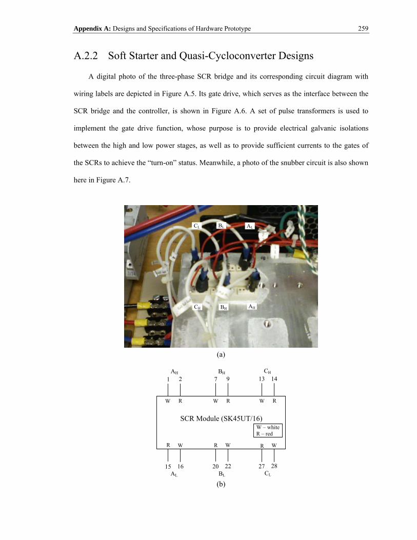
Appendix A: Designs and Specifications of Hardware Prototype
259
A.2.2 Soft Starter and Quasi-Cycloconverter Designs
A digital photo of the three-phase SCR bridge and its corresponding circuit diagram with
wiring labels are depicted in Figure A.5. Its gate drive, which serves as the interface between the
SCR bridge and the controller, is shown in Figure A.6. A set of pulse transformers is used to
implement the gate drive function, whose purpose is to provide electrical galvanic isolations
between the high and low power stages, as well as to provide sufficient currents to the gates of
the SCRs to achieve the “turn-on” status. Meanwhile, a photo of the snubber circuit is also shown
here in Figure A.7.
AHBHCH
ALBLCL
(a)
2
15
9
20
14
27
1
16
7 13
22 28
AH BH CH
AL BL CL
SCR Module (SK45UT/16)
W
W – white R – red
W W
W W W
R R R
R R R
(b)
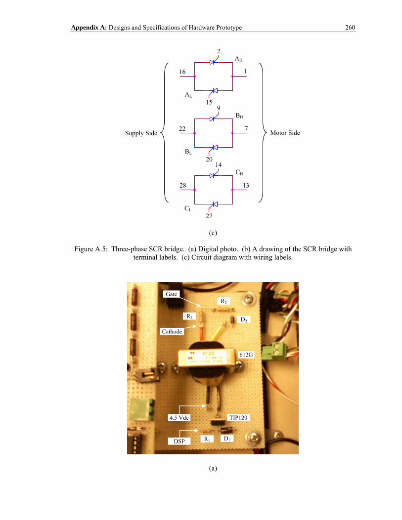
Appendix A: Designs and Specifications of Hardware Prototype
260
2
159
2014
27
116
7
13
22
28
Motor Side Supply Side
AH
BH
CH
AL
BL
CL
(c)
Figure A.5: Three-phase SCR bridge. (a) Digital photo. (b) A drawing of the SCR bridge with terminal labels. (c) Circuit diagram with wiring labels.
R1
R3 D2
R2
D1
TIP120
612G
Cathode
Gate
4.5 Vdc
DSP
(a)
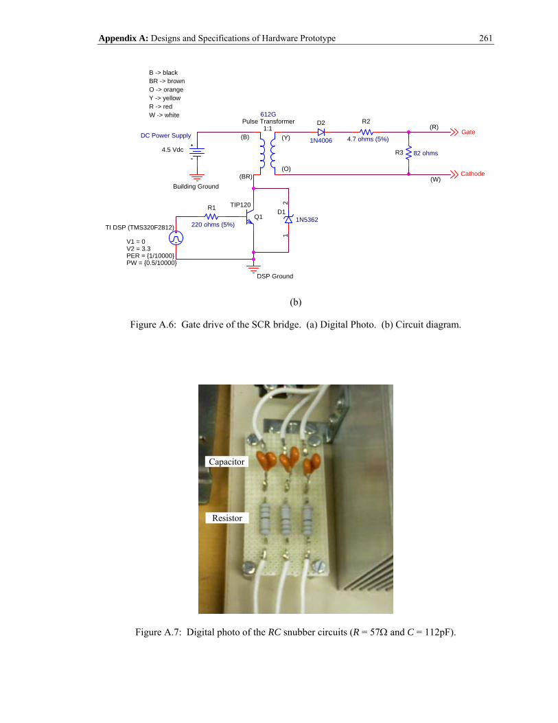
Appendix A: Designs and Specifications of Hardware Prototype
261
DC Power Supply
4.5 Vdc
Q1
1N4006
TI DSP (TMS320F2812)
Building Ground
82 ohms
220 ohms (5%)
Cathode(W)
DSP Ground
1:1D2 R2
R3
Gate
D1
(B) 4.7 ohms (5%)
(BR)
Pulse Transformer
(Y)
612G
B -> blackBR -> brownO -> orangeY -> yellowR -> redW -> white
1N5362
12
(O)
R1
(R)
TIP120
PW = 0.5/10000PER = 1/10000
V1 = 0V2 = 3.3
(b)
Figure A.6: Gate drive of the SCR bridge. (a) Digital Photo. (b) Circuit diagram.
Resistor
Capacitor
Figure A.7: Digital photo of the RC snubber circuits (R = 57Ω and C = 112pF).

Appendix A: Designs and Specifications of Hardware Prototype
262
A.2.3 PWM Drive
A digital photo of the three-phase PWM drive and its “closed-up” view are shown in Figure
A.8(a) and Figure A.8(b), respectively. A precharge device, which consists of a contactor and a
200Ω power resistor, is used to precharge the dc-link capacitors during the initial start-up. Both
the diode and inverter bridge are obtained from Semikron. In order to turn-on/off the IGBTs, a
Semikron gate drive is utilized to provide the interface between the IGBTs and the controller. The
block diagram and the connection schematics of the gate drive are depicted in Figure A.9. Since
the input to the gate drive for turning-on is 5V and turning-off is 0V, and the fact that the DSP
controller board only outputs PWM signal which goes from 0 to 3.3V, an opto-coupler is utilized.
Its purpose is to convert the 0 – 3.3V of the PWM signals from the DSP board to 0 – 5V to the
gate drive. The gate drive will then output the PWM signals to the IGBTs at -6.5V to +15V for
turning-off and turning-on, respectively. The circuit diagram of the opto-coupler is depicted in
Figure A.10.
A.2.4 DSP Controller Board
A digital photo of the Texas Instruments (TI) DSP board is shown in Figure A.11, and its
specifications are given in Table A.2.
Table A.2: Specifications of TI DSP board.
Generation TMS320F2812 CPU C28x, 32-bit, fixed-point Frequency 150 MHz PWM 16 channels ADC 16 channels at 12-bit each ADC Conversion Time 80 ns IO Supply / Core Supply 3.3 V / 1.9 V Flash 256 KB Timers 3 32-bit General-Purpose Timers

Appendix A: Designs and Specifications of Hardware Prototype
263
Resistor
Precharge Device
(a)
Diode Bridge
A B C
InverterBridge
(b)
Figure A.8: Photos of the PWM drive. (a) Drive and precharge device. (b) Closed-up view.
1
2
9
10
19
20
1
2
3
4
9
TopA BottomA TopB BottomB TopC BottomC
Primary
Secondary
(a)
1
2
9
10
19
20
TA TB TC
BA BB BCErr GND15V
+15V
(b) Note: GND15V is not tied to DSP Ground.
1
2
3
4
9
10Ω
EG
G = gate E = emitter
(c)
Figure A.9: Gate drive of the inverter bridge. (a) A drawing of the gate drive. (b) Primary side connection diagram. (c) Secondary side connection diagram.

Appendix A: Designs and Specifications of Hardware Prototype
264
1
2
3
4
8
7
6
5
HP2502
(a)
390 (10%)
7.5k (5%)DSP3.3V
(Blue)
DSPPWM
Signals(Red,White)
GND5V(Black)
5V(Blue)
To Inputs of Gate Drive(TA, BA, TB, BB, TC, BC)
2
3
8
6
5
HP2502
(b) Note: GND5V is not tied to DSP Ground.
Figure A.10: Opto-coupler. (a) Block diagram. (b) Circuit diagram (GND5V is tied to GND15V).
Figure A.11: DSP controller board.

Appendix A: Designs and Specifications of Hardware Prototype
265
A.2.5 Signal Conditioning Circuits
In this setup, there are two signal conditioning boards. The first board, which is depicted in
Figure A.12(a), consists of a set of three-phase measurement circuits of the supply voltages (see
Figure A.12(b) for per-phase circuit), a 1.5Volt dc-offset circuit (see Figure A.12(c)), an A/D
calibration circuit (see Figure A.12(d)), and a speed sensing circuit (see Figure A.12(e)). Since
the analog inputs of the DSP board only accept signals ranging from 0 to 3Volt, a 1.5Volt dc-
offset circuit is used here to provide the necessary dc offset to the measured ac signals (± 1.5V).
R1 R3
R2 R4
R5R6
R7
R8
U1
Vin
ABC
A
BC
R9
R10
R11
R12
R13
R16
ABC 2.2V1.5VSpeed_Out
R14
R15
D1
VREFSpeed_In
MeasuredVoltage
(a)
R5
1M
10k (1%)R6
R8
150k (1%)
U1
MAX41673
2
74
6
1
5+
-
V+
V-
OUT
OS1
OS2R2
1M
(Building Ground is tied to DSP Ground)
Analog Input to DSP
VREF
R1
1M(1% Precision Resistor)
Transformer Neutral = Building GroundDSP Ground
3.3Vdc
R7
150k (1%)
R4
1M
R3
1M
L-N Voltage
1.5 Vdc (Offset)
VinVout
(b)
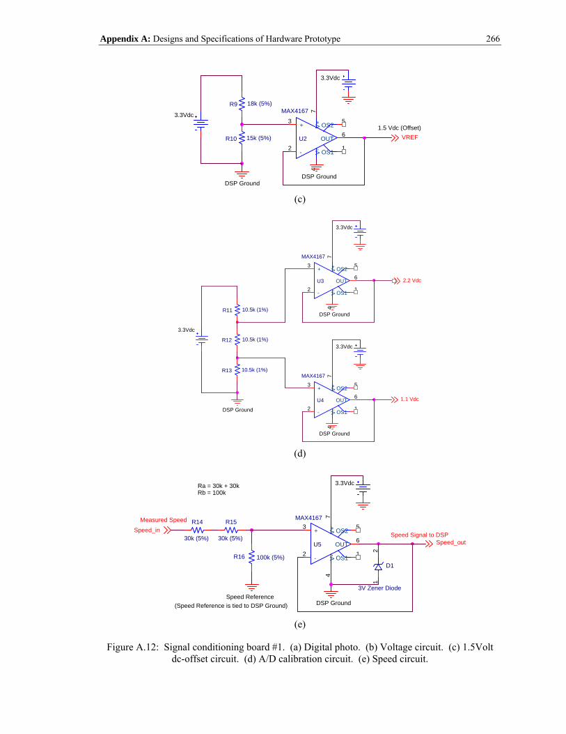
Appendix A: Designs and Specifications of Hardware Prototype
266
3.3Vdc
R9 18k (5%)
1.5 Vdc (Offset)
3.3Vdc
U2
MAX4167
3
2
74
6
1
5+
-
V+
V-
OUT
OS1
OS2
R10 15k (5%) VREF
DSP GroundDSP Ground
(c)
DSP Ground
DSP Ground
1.1 Vdc
R13 10.5k (1%)
R12 10.5k (1%)
U4
MAX41673
2
74
6
1
5+
-
V+
V-
OUT
OS1
OS2
2.2 VdcU3
MAX41673
2
74
6
1
5+
-
V+
V-
OUT
OS1
OS2
R11 10.5k (1%)
3.3Vdc
DSP Ground
3.3Vdc
3.3Vdc
(d)
R14
30k (5%)Speed_in
3V Zener Diode
D1
12
DSP Ground
Ra = 30k + 30kRb = 100k
Speed Reference
U5
MAX41673
2
74
6
1
5+
-
V+
V-
OUT
OS1
OS2
R16 100k (5%)
Measured Speed
Speed Signal to DSP
(Speed Reference is tied to DSP Ground)
R15
30k (5%) Speed_out
3.3Vdc
(e)
Figure A.12: Signal conditioning board #1. (a) Digital photo. (b) Voltage circuit. (c) 1.5Volt dc-offset circuit. (d) A/D calibration circuit. (e) Speed circuit.

Appendix A: Designs and Specifications of Hardware Prototype
267
Meanwhile, the second signal conditioning board, which is shown here in Figure A.13(a),
consists of a set of three-phase measurement circuits of the motor terminal voltages (see Figure
A.13(b) for per-phase circuit), a set of three-phase signal conditioning circuits for the motor phase
currents (see Figure A.13(c) for per-phase circuit), and a 1.5Volt dc-offset circuit (see Figure
A.13(d)).
R1 R3
R2 R4
R5 R6
R7
R8
U1
Vin
AB C
A
B C
A BC
MeasuredVoltage
VREF
R9
R10
R11
R12R13
R14
R15
3.3VGND
+15V -15V
A
C
right left
VOut
Current_In (Vin)
C1
C2
C3
Current_Out (VOut) Measured Current
B
(a)
Transformer Neutral = Building Ground
L-N Voltage
(Building Ground is tied to DSP Ground)VREF
3.3Vdc
(1% Precision Resistor)
Analog Input to DSP
1.5 Vdc (Offset)
DSP Ground
10k (1%)R6
Vout
R3
1M
C133uF
Vin
R7
150k (1%)
R1
1M
R2
1M
R8
150k (1%)
R4
1MU1
MAX41673
2
74
6
1
5+
-
V+
V-
OUT
OS1
OS2R5
1M
(b)
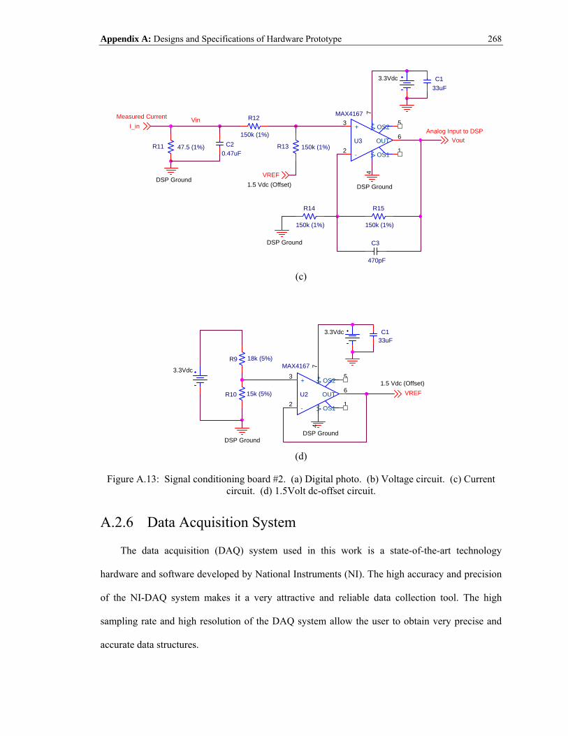
Appendix A: Designs and Specifications of Hardware Prototype
268
R13 150k (1%)
C3
470pF
Vin
R11 47.5 (1%)
Analog Input to DSP
Measured Current
DSP GroundDSP Ground
VREF
DSP Ground
1.5 Vdc (Offset)
U3
MAX41673
2
74
6
1
5+
-
V+
V-
OUT
OS1
OS2
R15
150k (1%)
3.3Vdc
R14
150k (1%)
R12
150k (1%)Vout
C133uF
C20.47uF
I_in
(c)
R9 18k (5%)
C133uF
DSP Ground
3.3Vdc
1.5 Vdc (Offset)
R10 15k (5%) U2
MAX4167
3
2
74
6
1
5+
-
V+
V-
OUT
OS1
OS2
3.3Vdc
VREF
DSP Ground (d)
Figure A.13: Signal conditioning board #2. (a) Digital photo. (b) Voltage circuit. (c) Current circuit. (d) 1.5Volt dc-offset circuit.
A.2.6 Data Acquisition System
The data acquisition (DAQ) system used in this work is a state-of-the-art technology
hardware and software developed by National Instruments (NI). The high accuracy and precision
of the NI-DAQ system makes it a very attractive and reliable data collection tool. The high
sampling rate and high resolution of the DAQ system allow the user to obtain very precise and
accurate data structures.

Appendix A: Designs and Specifications of Hardware Prototype
269
The DAQ system uses an E-Series technology (PCI-6052E) to deliver high performance,
reliable data acquisition capabilities to meet a wide range of application requirements. It provides
a sampling rate of 333 kSamples/sec and 16-bit resolution on 16 single-ended analog inputs.
Depending on the type of hard disk of the computer, the NI PCI-6052E can stream to hard disk at
rates up to 333 kSamples/sec. This DAQ board features analog and digital triggering capability,
as well as two 24-bit, 20 MHz counter/timers, 8 digital Input/Output (I/O) lines, and two 16-bit
analog outputs. Table A.3 summarizes the overall features of this DAQ system.
Table A.3: Features of NI DAQ system.
Family PCI-6052E Bus PCI Analog Input 16 Single-Ended Resolution 16 Bits Sampling Rates 333 kSamples/sec Input Range ± 0.05 to ± 10 Volts Analog Output 2 Resolution 16 Bits Output Rate 333 kSamples/sec Output Range ± 10 Volts Digital I/O 8 Counter / Timers Two 24 Bit, 20 MHz Triggers Analog and Digital


![PROFICIENTLY DRIVE YOUR [PM OPERATIONS]](https://img.pdfslide.net/doc/110x75/629b29fb708a441d652f4ce3/proficiently-drive-your-pm-operations.jpg)