1

High Performance Computing on GPU Clusters

Timothy McGuinessa, Ali Khajeh-Saeed

b, Stephen Poole

c and J. Blair Perot

b

aLincoln Laboratories, Lexington, MA, 02420, USA

bDepartment of Mechanical and Industrial Engineering, University of Massachusetts, Amherst, MA, 01003, USA cComputer Science and Mathematics Division, Oak Ridge National Laboratory, Oak Ridge, TN 37831, USA

Abstract

Commodity graphics cards have recently proven to be an inexpensive and effective way to accelerate some

scientific computations. Acceleration using multiple GPUs is more challenging, because the type of

algorithm/parallelism needed to couple many GPUs is very different from the algorithm/parallelism used to

efficiently utilize a single GPU. In this work, four very different applications are evaluated in both the

single and multiple GPU contexts. The algorithms are memory bound, like almost all scientific computing

algorithms. But the memory use differs considerably allowing us to isolate which types of scientific

computing algorithms are likely to benefit from GPU acceleration, and which problems are more easily

solved on traditional CPU clusters.

Keywords: GPGPU, STREAM Benchmark, Smith-Waterman, Graph Analysis, Unbalanced Tree Search.

1. Introduction

The early 2000s saw the development of several high-level shading languages such as Cg [1], HLSL and

OpenGL [2], designed to help exploit the computational power of graphics hardware. These languages

dealt heavily in graphics-specific concepts such as textures and fragments, making it necessary for

scientific programmers to navigate an additional level of abstraction [3]. In late 2006, NVIDIA released

their Compute Unified Device Architecture (CUDA), providing a much more user-friendly general purpose

GPU (GPGPU) programming environment. Using only a few extensions to the C language, CUDA allows

programmers to easily create code for execution on graphics hardware. Even more recently OpenCL has

been introduced allowing code to be written for any GPU hardware.

When used as a math accelerator for scientific algorithms, single GPUs often produce roughly an order of

magnitude performance increase over a similar generation dual or quad core CPU. The tradeoff involved

with GPU computing is that programming efficient code is more difficult, and the hardware is more

specific about when it performs well. This work is intended to delineate the region of applicability of GPU

hardware more definitively. We will show some cases with over 100x speedup over a CPU, and some

which show (despite our best efforts) a performance decrease compared to the CPU. The benchmarks

chosen for this study are interesting because they span a range of applications from very linear memory

access patterns, to regular but non-linear access patterns, to entirely random memory access dominated

algorithms.

This work also explores the algorithmic changes necessary to efficiently program software to use GPU

clusters with hundreds of GPUs. Because of its popularity, this work uses MPI (Message Passing Interface)

as the communication protocol between the GPUs. The paper also explores the performance of GPU

clusters based on dedicated scientific computing GPUs (Tesla), and a cluster built from the lower cost

commodity GPUs (GTX 295 and 480).

The four benchmarks were chosen to span a wide range of different scientific computing applications. The

STREAM benchmark accesses double precision memory linearly. It scales almost directly with the linear

memory access speed of the hardware, and provides an upper bound on the power consumption and

temperature limits achieved by the GPUs. Our next benchmark, DNA sequencing via the Smith-Waterman

algorithm, deals with sequence matching for very large sequences. This task is represented by the Scalable

Synthetic Compact Application (SSCA) #1 benchmark which performs different variants of the Smith-

Waterman algorithm. The classic Smith-Waterman algorithm fills in a large table one anti-diagonal row at

2

a time. When reformulated for the GPU architecture this benchmark shows 100x and 70x speedup over a

single core of a CPU for single GTX 480 and GTX 259 GPU, and a 5335x speedup when using 120 GPUs

(44x faster than a single GPU). The third application is the HPCS SSCA #2 benchmark which analyzes

very large graphs consisting of a set of nodes connected by a set of edges. Graphs are directed and

weighted, meaning edges have specific start and end nodes, as well as a given cost or weight value. This

application depends almost entirely on random memory accesses. Finally, the unbalanced tree search

displays both random memory accesses and the need for dynamic load balancing, since the tree is so large

it must be built „on the fly‟. We describe load balancing techniques both on a single GPU and when using

many GPUs.

Two machines were used for computations, Orion and Lincoln. Orion contains an AMD quad-core Phenom

II X4 CPU, operating at 3.2 GHz, with 4 x 512 KB of L2 cache, 6 MB of L3 cache and 8 GB of RAM. In

terms of GPUs, Orion contains four NVIDIA 295 GTX cards (occupying four PCIe 16x slots) which each

come as two GPU cards sharing a single PCIe slot. When we refer to a single 295 GTX GPU we refer to

one of these two cards, which has 240 cores and a memory bandwidth of 111.9 GB/s. Orion therefore

typically has 8 GPUs. Also we replaced the first and second GPUs with GTX 480 and Tesla C2070 cards

in order to run some cases with these new GPUs. Orion is shown in figure 1. Results on Orion were

compiled using Microsoft Visual Studio 2005 (VS 8) under Windows XP Professional x64. The bulk of

NVIDIA SDK examples use this configuration.

Figure 1. Orion configuration and fan locations (Fan 6 is located on the side of the case, blowing air into the GPUs)

Lincoln is a Teragrid/XSede GPU cluster located at NCSA. Lincoln has 96 Tesla S1070 (384 GPUs).

Lincoln‟s 192 servers each hold two Intel 64 (Harpertown) 2.33 GHz dual socket quad-core processors

with 2 x 6 MB L2 cache and 2 GB of RAM per core. Each server is connected to 2 Tesla processors via

PCI-e Gen2 X8 slots. All code was written in C++ with NVIDIA‟s CUDA language extensions for the

GPU. The Lincoln results were compiled using Red Hat Enterprise Linux 4 (Linux 2.6.19) and the gcc

compiler [4].

2. STREAM Benchmark

The STREAM benchmark is a simple synthetic benchmark program that measures sustainable memory

bandwidth (in MB/s) and the corresponding computation rate for simple vector kernels. The STREAM

benchmark is composed of four kernels. In the first kernel one vector is copied to another within the same

device (a = b, one read and one write). For the second kernel, vector entries are multiplied by a constant

number and the results is written to another vector (a = b, one read and one write). Kernel 3 adds two

3

vectors (a = b + c, two reads and one write). Finally, Kernel 4 is a combination of Kernels two and three,

sometimes referred to as a DAXPY operation (a = b + c, two reads and one write).

This benchmark was computed using a single GPU operating on different vector sizes. Table 1 shows the

specifications for four types of NVIDIA GPUs. The GTX 295 and Tesla S1070 actually house two and four

GPUs respectively. However the hardware specifications below are for one of these GPUs (1/2 of the 295

GTX and 1/4 of the Tesla S1070) [5, 6]. The GTX 480 and Tesla C2070 are the latest generation of GPUs

(Fermi architecture). The tests shown below used 64k blocks with 128 threads each, operating on double

precision vectors. Each GPU kernel was called 100 times, and each kernel performs the STREAM

operation 100 times in that kernel. The timings below are reported for a single STREAM operation (total

time / 10,000).

Table 1. NVIDIA hardware specifications for four different GPUs

2.1 Single GPU

Figures 2 and 3 show the single-GPU execution time and bandwidth for the GTX 295 and 480 GPU and

Tesla S1070 and C2070. For vectors with lengths less 105

elements, the time is nearly constant and the

bandwidth is less than the maximum value for 10 series and 20 series respectively. However, for vector

sizes larger than 105 the bandwidth is close too the maximum value and execution time increases linearly

with vector length. This shows that the startup cost of simply initiating a GPU kernel is high, and large

vector lengths are required for good GPU performance.

Vector Length

Tim

e(m

s)

102

102

103

103

104

104

105

105

106

106

107

107

108

108

109

109

10-3

10-3

10-2

10-2

10-1

10-1

100

100

101

101

102

102

Copy (GTX 295)

Scalar (GTX 295)

Add (GTX 295)

TriAdd (GTX 295)

Copy (GTX 480)

Scalar (GTX 480)

Add (GTX 480)

TriAdd (GTX 480)

Vector Length

Ba

nd

wid

th(G

B/s

ec)

102

102

103

103

104

104

105

105

106

106

107

107

108

108

109

109

10-1

10-1

100

100

101

101

102

102

103

103

Copy (GTX 295)

Scalar (GTX 295)

Add (GTX 295)

TriAdd (GTX 295)

Copy (GTX 480)

Scalar (GTX 480)

Add (GTX 480)

TriAdd (GTX 480)

Figure 2. (a) Time and (b) Bandwidth for single NVIDIA GTX 295 and GTX 480 for the different STREAM kernels.

The Tesla S1070 has more memory (4 GB) than the 295 GTX (896 MB). However, Figure 3 shows that for

large vector lengths (greater than 5×107) bandwidth begins to decrease. For the largest possible lengths on

the Tesla S1070, bandwidth is approximately 50% of the maximum value. However, there is no efficiency

loses for Tesla C2070 when using large vector sizes. Also figure 3 shows that for small problem sizes Tesla

S1070 has better performance than C2070. The kernel startup time for the C2070 is an order of magnitude

Model CUDA

Cores

Memory

(MB)

Theoretical

Bandwidth (GB/sec)

Memory Interface

Width (bits)

Max Power

(W)

GTX 295 240 896 119.9 448 145

GTX 480 480 1536 177.4 384 250

Tesla S1070 240 4000 102 512 200

Tesla C2070 448 6000 144 384 238

(a)

(b)

4

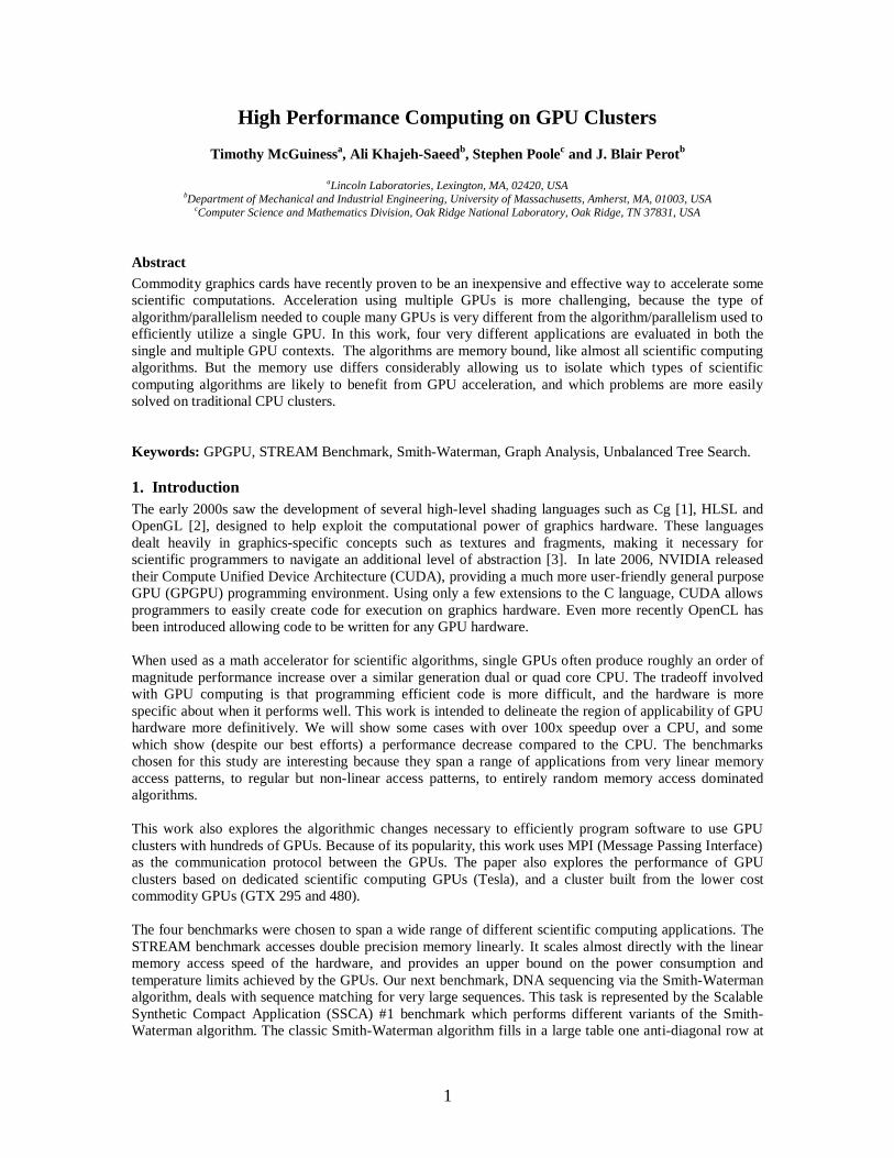
larger than its predecessor. The bandwidth achieved by the STREAM benchmark is consistently about 20%

below the theoretical peak predicted by Nvidia for all GPUs.

Vector Length

Tim

e(m

s)

102

102

103

103

104

104

105

105

106

106

107

107

108

108

109

109

10-3

10-3

10-2

10-2

10-1

10-1

100

100

101

101

102

102

103

103

Copy (Tesla S1070)

Scalar (Tesla S1070)

Add (Tesla S1070)

TriAdd (Tesla S1070)

Copy (Tesla C2070)

Scalar (Tesla C2070)

Add (Tesla C2070)

TriAdd (Tesla C2070)

Vector Length

Ba

nd

wid

th(G

B/s

ec)

102

102

103

103

104

104

105

105

106

106

107

107

108

108

109

109

10-1

10-1

100

100

101

101

102

102

103

103

Copy (Tesla S1070)

Scalar (Tesla S1070)

Add (Tesla S1070)

TriAdd (Tesla S1070)

Copy (Tesla C2070)

Scalar (Tesla C2070)

Add (Tesla C2070)

TriAdd (Tesla C2070)

Figure 3. Time and bandwidth for single NVIDIA Tesla S1070 and C2070 for four different STREAM kernels

2.2 Weak Scaling on many GPUs

In the weak scaling case, the vector length is constant per GPU (at 2M double precision elements). This

makes the number of operations constant per GPU as the number of GPUs increases. Figure 3 shows the

results for weak scaling. Figures 4a and 4b show total bandwidth as well as bandwidth per GPU for various

numbers of GPUs. Because 2M is large enough for a single GPU to be efficient, the bandwidth is close to

the maximum value and the speedup is linear.

Number of GPUs

Ba

nd

wid

th(G

B/s

)

0 8 16 24 32 40 48 56 640 0

1000 1000

2000 2000

3000 3000

4000 4000

5000 5000

6000 6000

7000 7000

Copy

Scalar

Add

TriAdd

Ideal

Number of GPUs

Ba

nd

wid

th/G

PU

(GB

/s)

0 8 16 24 32 40 48 56 640 0

20 20

40 40

60 60

80 80

100 100

120 120

Copy

Scalar

Add

TriAdd

Ideal

Figure 4. Results for weak scaling of the four STREAM benchmark kernels on Lincoln with 2M elements per GPU,

(a) Actual and ideal bandwidth for various numbers of GPUs, (b) bandwidth per GPU for various numbers of GPUs.

2.3 Strong Scaling

In the strong scaling case, vector length remains constant, and number of processors varies. This means

increased number of GPUs decreases the vector length per GPU. The total vector length used for the strong

scaling case was 32M. This results in 0.5M elements per GPU when 64 GPUs are used for the computation.

Figures 5a and 5b show MCUPS (millions of cell updates per second) and bandwidth per GPU for various

numbers of GPUs, respectively. Small numbers of GPUs are less efficient for this case because memory

accesses are slow because the vector length is so large (greater than 107, see figure 3b).

(a)

(b)

(a)

(b)

5

Number of GPUs

MC

UP

S

10 20 30 40 50 6010

310

3

104

104

105

105

106

106

Copy

Scalar

Add

TriAdd

Number of GPUs

Ba

nd

wid

th/G

PU

(GB

/s)

0 8 16 24 32 40 48 56 640 0

20 20

40 40

60 60

80 80

100 100

120 120

Copy

Scalar

Add

TriAdd

Ideal

Figure 5. Results of strong scaling of the four STREAM benchmark kernels on the Lincoln with 32M total elements,

(a) MCUPS for different numbers of GPUs, (b) bandwidth per GPU for various numbers of GPUs.

2.4 Power Consumption

Figures 6a and 6b show power consumption for the AMD quad-core Phenom II X4, operating at 3.2 GHz,

and for the GTX 295 GPUs, respectively. This test involved the STREAM Benchmark operating on double

precision vectors of length 2M per GPU. Power was measured at the source to Orion using a watt meter.

Note that 60 W (for figure 6a) is not what the whole machine draws when running idle. At idle it draws

close to 450 W (there are many fans).

Number of Cores (CPU)

Wa

tt

0 1 2 3 4 550 50

60 60

70 70

80 80

90 90

100 100

110 110

120 120

Watt = 12.3 x (Cores) + 60

Number of GPUs

Wa

tt

0 2 4 6 8 100 0

200 200

400 400

600 600

800 800

1000 1000

1200 1200

Watt = 115 x (GPUs) + 31

Figure 6. Power consumption for the weak scaling STREAM benchmark on Orion with the AMD CPU and 295 GTX GPUs.

Each GPU uses approximately 115 W over idle consumption when running the STREAM Benchmark.

Also, it was found that the idle power for one GTX 295 (2 GPUs) is 71 W (or about 30 W per GPU). This

was ascertained by physically removing GPUs from the machine, and re-running the code. The NVIDIA

hardware specifications (table 1) imply that each Tesla S1070 GPU uses more power than the GTX 295

GPUs (200 W vs. 145 W maximum). One reason for this difference could be the amount of memory

supported. The Tesla S1070 has 4000 MB per GPU but the GTX 295 has only 896 MB per GPU. The Tesla

also contains its own power supply and cooling system, which may be playing a role in the difference in

consumption levels. We did not have access to the Tesla hardware (at NCSA) to measure its power

consumption directly.

(a) (b)

(a) (b)

6

2.5 GPU Temperature

The STREAM benchmark was computed on Orion (GTX 295 GPUs) to obtain a measurement of each

GPU‟s temperature. The code was run with 8 GPUs for 331 seconds. Table 2 shows the initial and

maximum temperatures for each GPU, as the STREAM benchmark was running for 331 seconds. The

maximum allowable temperature for the 295 GTX listed on NVIDIA‟s website is 105 oC [5]. The

maximum GPU temperatures range between 88-96 oC when running for this prolonged period of time.

Since most GPGPU applications involve many short kernel calls rather than this type of extended exertion,

GPU temperatures are typically lower than these maximum measured values.

Table 2. Temperatures for GTX 295 cards, running for 331 second STREAM benchmark

Temperature GPU 1 GPU 2 GPU 3 GPU 4 GPU 5 GPU 6 GPU 7 GPU 8

Initial Temp oC 66 64 72 68 72 67 63 61

Max Temp oC 90 88 96 92 96 93 91 88

T oC 24 24 24 24 24 26 28 27

3. SSCA #1 – Sequence Matching

For two candidate sequences, A and B, sequence alignment attempts to find the best matching

subsequences for the pair. The best match is defined in equation 1,

1

( ), ( ) ,L

s eiS A i B i W G G

(1)

where W is a gap function involving the gap start- and gap extension-penalties, (Gs and Ge, respectively)

and the similarity score S, which is user-defined for this implementation. This research uses a simple

scoring system where matching items get a score of 5 and non-matching items have a score of -3. The gap

start-penalty is 8 and gap extension-penalty is 1.

The Smith-Waterman algorithm locates the optimal alignment by building a solution table [8]. The first

data sequence (the database) is typically seeded along the top row, with the second sequence (the test

sequence) in the first column. Table values are denoted as ,i jH with i and j being the row and column

indices, respectively. Other table entries are set using the equation,

1, 1 ,

, ,0

,0

,0

( )

( )

i j i j

i j i k j s ek i

i j k s ek j

Max H S

H Max Max H G kG

Max H G kG

(2)

That is, an entry in the table is the maximum of: the entry diagonally to the upper left plus the similarity

score for the item in that row and column, the maximum of all the entries above the entry and in that same

column minus a gap function, and the maximum of all the entries to the left of the entry and in that same

row minus a gap function, and zero. It is not possible for table values to be negative. Additionally, the

dependencies of table values are such that they cannot be computed in parallel. Finding a particular value in

the table requires knowledge of all the values above and to the left of the value being computed. Figure 7

shows table value dependencies.

7

If equation (2) is naïvely implemented, then the column and row maximums (second and third items in

equation (3) are repetitively calculated for each table entry creating O(L1L2(L1+L2)) computational work.

This can be reduced by retaining the previous row and column sums [9] which reduces the work

significantly but triples the algorithm‟s required storage space. The classic parallelization technique for this

algorithm is to work along anti-diagonals [10]. It should be clear from the dependency region that each

diagonal item can be calculated independently of the others. This means the diagonal algorithm only

performs efficiently on a single GPU when the shorter of the two sequence lengths is 30k or larger.

Sequence lengths of this size are uncommon in biological applications, but this is not the true problem with

the diagonal algorithm. The primary issue with the diagonal approach is memory accesses patterns. On the

GPU it is very efficient to access up to 32 consecutive memory locations, and relatively (5-10x slower)

inefficient to access random memory locations such as those dispersed along the anti-diagonal (and its

neighbors). To get around this problem, it was shown that the Smith-Waterman algorithm can be

reformulated so calculations can be performed simultaneously one row (or column) at a time [11, 12]. Row

(or column) calculations allow GPU memory accesses to be consecutive, and therefore fast.

3.1 Results

The first kernel computes the Smith-Waterman table is saves the largest table values (200 of them) and

their locations. These serve as the end points of well-aligned sequences, but the sequences themselves are

not constructed or saved until Kernel 2. Because the traceback step is not performed in Kernel 1, the

amount of data needed in GPU memory from the table is minimal. For example, in the row-parallel version,

only the data from the previous row needs to be retained, making Kernel 1 both memory-efficient and

highly parallel on a fine scale. The results for four different GPUs are shown in Fig. 8. The weak scaling

timings are shown in Fig. 9a, for the case using a 2M-elements database per GPU, and a 128-element test

sequence. Obviously, the amount of work being performed increases proportionally with the number of

GPUs used. The total times are from 380–480 ms, and they increase slowly with the number of GPUs used.

Figure 9b shows speedups for Kernel 1 compared to a single-CPU version. Compared to a single core of

the CPU, the speedup is 100x for a single GPU, and 5335x for 120 GPUs. Figures 10a and 10b show

speedups for Kernel 2. Kernel 2 is not very sensitive to sequences length and does not show nearly as large

of a speedup. The complexity of kernel 2 means that the GPU performs at roughly the same speed as all the

cores on the CPU.

0 C A G C C U C G C U G

0 0 0 0 0 0 0 0 0 0 0 0 0

A 0 0 5 0 0 0 0 0 0

A 0 0 5 2 0 0 0 0 0

U 0 0 0 2 0 0 5 0 0

G 0 0 0 5 0 0 0 2 5

C 0 5 0 0 10 5 0 5 0

C 0 5 2 0 5 15 6 5 4

A

U

G

C

G

Figure 7. Dependency of the values in the Smith-Waterman table.

8

Size

Tim

e(s

)

106

107

108

109

1010

1011

10-1

10-1

100

100

101

101

102

102

103

103

104

104

9800 GT

9800 GTX

295 GTX

Tesla S1070

480 GTX

CPU 3.2 MHz

Size

Sp

ee

du

p

106

107

108

109

1010

1011

0 0

20 20

40 40

60 60

80 80

100 100

120 120

9800 GT

9800 GTX

295 GTX

Tesla S1070

480 GTX

Figure 8. Results for four different GPUs timings (a) and speedups (b) for Kernel 1.

Kernel 1 performed particularly well on the GPU for the SSCA #1 benchmark because it was possible to

reformulate the Smith-Waterman algorithm to use sequential stride 1 memory accesses. Since each

sequential memory access can be guaranteed to come from a different memory bank these accesses will

occur simultaneously. The parallel scan was a critical component of being able to perform this

reformulation. The parallel scan operation may currently be under-utilized and might be effectively used in

many other scientific algorithms as well.

On the other hand, the speedups demonstrated by the already very fast Kernel 2 were not as impressive.

The naïve algorithms for these tasks are parallel but also MIMD. Because this kernel executes so quickly

already there was little motivation to find SIMT analogs and pursue better GPU performance. Fortunately,

every GPU is hosted by a CPU, so users are not forced to use a GPU if the task is not well suited to the

hardware. It is important to keep in mind that the GPU is meant to be a supplement to the CPU. This paper

is intended to give the reader insight into which types of tasks will do well when ported to the GPU and

which will not.

Number of GPUs

Ke

rne

l1

Tim

e(m

s)

0 20 40 60 80 100 120300

320

340

360

380

400

420

440

460

480

500

Number of GPUs

Ke

rne

l1

Sp

ee

du

p

0 20 40 60 80 100 1200

500

1000

1500

2000

2500

3000

3500

4000

4500

Figure 9. Weak scaling timings (a) and speedups (b) for Kernel 1 using various numbers of GPUs on Lincoln.

(a) (b)

(a) (b)

9

Number of GPUs

Ke

rne

l2

Tim

e(m

s)

0 20 40 60 80 100 1200

5

10

15

20

25

30

Number of GPUs

Ke

rne

l2

Sp

ee

du

p

0 20 40 60 80 100 1200

0.5

1

1.5

2

2.5

3

3.5

4

4.5

5

5.5

6

Figure 10. Weak scaling timings (a) and speedups (b) for Kernel 2 using various numbers of GPUs on Lincoln.

The issue of programming multiple GPUs is an interesting one, because it requires the use of a totally

different type of parallelism. A single GPU functions well with massive fine grained (at least 30k threads)

nearly SIMD parallelism. With multiple GPUs, located on different computers, communicating via MPI

and Ethernet cards, course grained MIMD parallelism is needed. Due to this, all multi-GPU

implementations partition the problem coarsely into subsets for the GPUs, and then use fined grained

parallelism within each GPU.

4. SSCA #2 – Graph Analysis

The graphs for this benchmark consist of a set of nodes, connected by a set of directed edges. The size of

the graph is given by the user-defined variable SCALE. The number of nodes in the graph is 2SCALE

, and the

number of edges is eight times the number of nodes [13]. A node‟s degree value is the number of edges

pointing out from it. Because there are eight times as many edges as nodes, the average nodal degree is

eight. The histogram in figure 11 shows the number of nodes for any given degree value. Graphs are

constructed so that there are a few nodes with very high degrees. These graphs are examined using four

timed kernels, described in the following sections.

Figure 11. Statistical distribution of edges for a typical SCALE 21 graph.

4.1 Kernel 1 – Graph Construction

The original edge list is presented as three lists; start node, end node and edge weight. The purpose of the

first kernel is to convert this data structure into the format that the remaining kernels will use. The graph

may be represented in any format, but this new data structure cannot be altered after Kernel 1.

(a) (b)

10

The new structure used in the GPU code is a node-to-node (N2N) system. This structure uses two arrays – a

shorter list of pointers, and a longer list of children. In the pointer list, the entry at position p is a location q

in the child array; the location where parent p‟s children are saved. The pointer list is „number of nodes‟

long, since each node in the graph can be treated as a parent, and the child list is „edges‟ long, because it

stores all the end nodes from the original edge list. A simple way to think of building N2N, is by sorting the

original list according to start node. In this case, the list of start nodes would then consist of large groups of

1‟s, 2‟s, 3‟s, etc. This array is condensed into a list of where the 1‟s, 2‟s and 3‟s – and hence, their children

– begin. An illustration of this conversion is shown in figure 12.

Figure 12. Conversion from (a) original edge list, to (b) sorted by start node, and finally to (c) N2N format.

The code performs this conversion in three steps. First, nodal degrees are counted by looping over each

edge, and incrementing an array of counters corresponding to start nodes. Next, this list of degrees is

converted into the pointer list, using an operation known as a parallel scan [14]. The scanned pointer value

for a node is the sum of the degree values for all preceding nodes. The final step builds the child list using

the newly created pointer list. A loop finds each edge‟s start node and the corresponding pointer, and

inserts the edge‟s end node into the child array at that location. Care must be taken to offset individual end

nodes from the pointer to ensure unique locations in the child list.

It is worth nothing that Kernel 1 not only builds the standard N2N structure, which follows the true

direction of the edges (N2Nout), but it also builds a second N2N structure that goes “against the grain”

(N2Nin). This second version has proven useful for the parallel implementations of Kernels 2 and 4.

4.2 Kernel 2 – Find Max-Weight Edges

Kernel 2 searches through edge weights and picks out those with the largest possible value. The use of the

N2N data structure actually makes this task more challenging. In the original edge list, weights are paired

with data for both nodes. In the new structure, weights are only associated with one node, and finding the

second is non-trivial.

For this algorithm, threads search the weight list in the N2Nin structure for max-weight values. When a

max-weight is found, the corresponding node (the edge‟s start node) is saved. Using this node and the

N2Nout pointer list, the GPU finds the location of that node‟s children, and searches this limited region for a

max-weight edge. When the weight is found, the corresponding node (the edge‟s end node) is paired with

its start node.

Due to the benchmark‟s specifications regarding number of edges and weight distribution, there are on

average only eight max-weight edges in any graph, regardless of SCALE. As a result, this kernel has

relatively little work to do, and is easily the fastest of the four timed tasks.

4.3 Kernel 3 – Subgraph Construction

The third kernel of SSCA 2 is designed to construct subsets (or subgraphs) of the original graph, using the

edges found in Kernel 2 as starting points. Kernel 3 starts at a max-weight edge, and moves out a user-

specified number of levels from it.

11

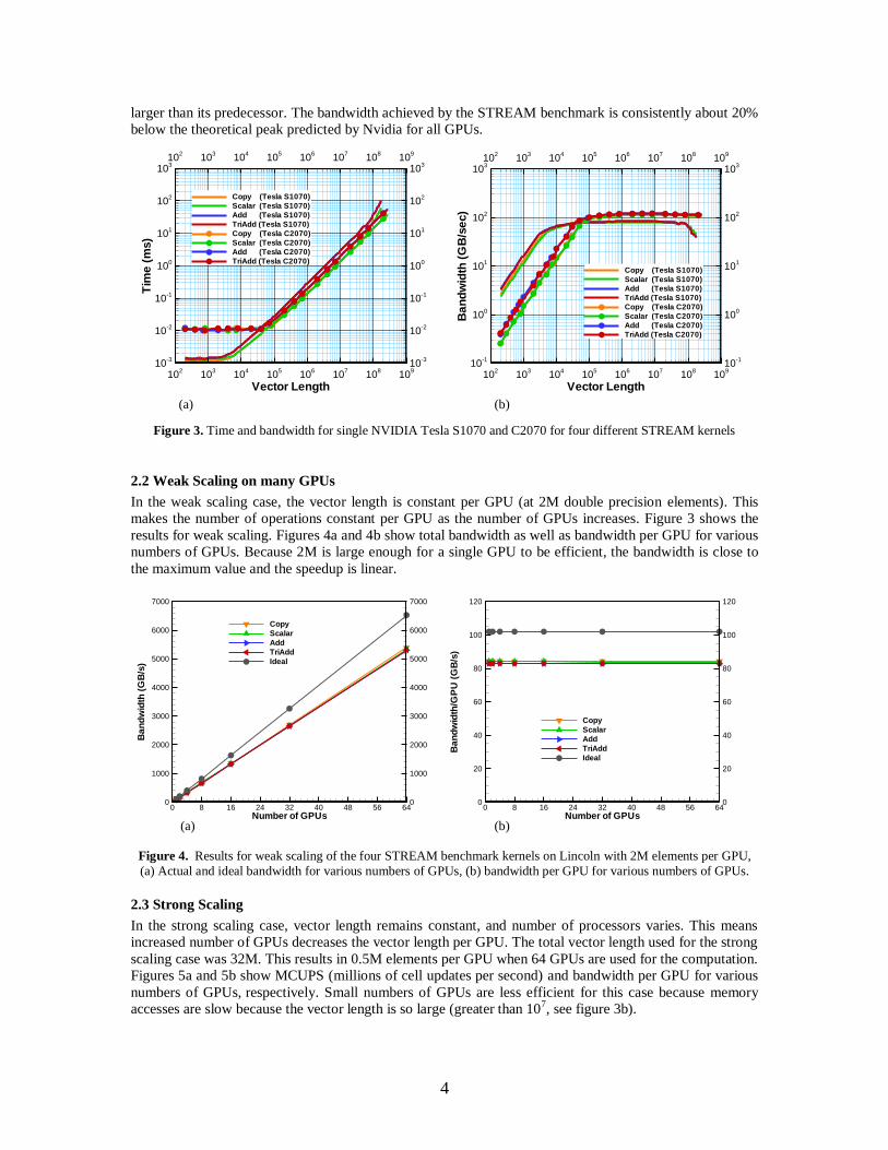
The final output of Kernel 3 is a list of nodes which representing the members of the subgraph. This list,

called the queue, is built in sections, which are filled as the code steps out to each new level of the

subgraph. The code reads parent nodes from the current level, and fills in their children in the next level.

The most challenging part of parallelizing this code is determining where to insert children into the queue.

Each thread needs its own dedicated space in the queue, and must know where that space begins. This is

done by storing count and point arrays which correspond to the queue. When a node is added to the queue,

its number of children is recorded in the count array. After each level is filled, this array is scanned into the

point array, which then tells the queue location for that node‟s children. This process is illustrated in figure

13. Before a child is inserted into the queue, the code tests to ensure it has not already been added. This

eliminates extraneous queue entries, limits the amount of required memory, and provides a natural stopping

point for the following kernel.

Figure 13. Construction of the Kernel 3 queue. (a) the first node in the queue, with its number of children, and the

location they will be written to, (b) the second generation, and the scanned point array (c) part of the third generation.

4.4 Kernel 4 – Betweenness Centrality

The goal of Kernel 4 is to determine which nodes have the highest connectivity, or betweenness centrality

(BC). For a particular starting node, partial BC scores are calculated for all other nodes. This process is

repeated using a subset of nodes as starting points. A node‟s final BC value is the sum of all its partial

scores. This is easily the most computationally-taxing portion of the SSCA 2 code.

As proposed by Brandes [15], and Bader and Madduri [16], the BC algorithm consists of two main steps.

The outsweep assigns nodal values of distance to and number of shortest paths back to the start node. This

process is conducted in the same manner as Kernel 3, moving out visiting new generations, level by level.

The only differences are nodal values need to be assigned now in addition to just filling the queue, and the

algorithm must continue for as long as it takes to visit all nodes. Assigning depth and shortest path values is

trivial, and since each node can only appear once in the queue, the final queue level will be empty, and the

algorithm will stop on its own.

The insweep works through the queue backwards, level by level. As the code moves in (from child to

parent) along shortest paths, the child‟s BC and shortest paths values are used to update the BC score for

the parent. The N2Nin data structure – carefully marked during the outsweep – is used to determine if

parents lie along these shortest paths. In equation 3, υ and ω represent parent and child nodes, respectively.

A node‟s temporary BC score (reset after each outsweep / insweep pair) is represented by δ, while σ is a

node‟s shortest path value.

1

(3)

One of the problems frequently encountered during SSCA 2 is when multiple GPU threads attempt

simultaneous reads or writes to the same memory location. This never occurs in serial versions since only a

single core is active, working on a single data element. The simplest solution to this problem is atomic

functions, which are built into the CUDA API. These perform a simple locking procedure to serialize all

12

threads in the device attempting concurrent reads/writes. These are essential to several parts the SSCA 2

code – particularly for finding nodal degrees in Kernel 1. However, these operations only work with integer

values, and are therefore, limited.

4.5 Results

The parallel SSCA #2 code uses MPI to run on up to 128 GPUs simultaneously. Comparisons to a single

CPU refer to the HPCS optimized code provided with the benchmark. The GPU timings reported in figure

14 are from trials conducted on the Lincoln cluster. Results on up to four cards on the Orion machine can

be found in [17].

Number of GPUs

Sp

ee

du

p(C

PU

)

10-1

100

101

102

10310

0

101

102

103

Kernel 1

Kernel 2

Kernel 3

Kernel 4

Number of GPUs

Sp

ee

du

p(G

PU

)

10-1

100

101

102

10310

-1

100

101

102

103

Kernel 1

Kernel 2

Kernel 3

Kernel 4

Figure 14. Strong scaling speedups for Kernels 1–4 (a) relative to a single CPU core,

and (b) relative to a single GPU. All tests were run for a SCALE 21 graph.

The results are also compared with HPC CPU code that is optimized for multi-core CPUs. Figure 15 shows

that with equal number of GPUs and CPU cores, we achieved 30, 0.4 and 4 speedup for Kernel 1, 3 and 4

respectively. Kernel 4 is by far the most computationally demanding of the four kernels and only shows a

speed up of 4. This means the GPU is performing roughly like a quad-core CPU for this benchmark.

GPUs

Sp

ee

du

p

2 4 6 8 10 12 14 161810

-110

-1

100

100

101

101

102

102

Kernel 1

Kernel 3

Kernel 4

Figure 15. Speedup for GPUs comparing with equal number of CPU cores with HPC code

Several important conclusions can be drawn from this data. First, GPU performance is better for larger

problem sizes. This is a trend that is clearly evident when speedups are compared for multiple SCALEs,

and when GPU and CPU results are directly compared (not pictured). For small graphs, the GPU was not

able to produce the expected speedups, however as SCALE size increased, timings began moving closer to

the theoretical performance. In Kernel 2, each GPU operates on a portion of the N2N list. As the number of

(a) (b)

13

GPUs increases, the workload decreases. The results in figure 8 show that for fewer GPUs, Kernel 2‟s

performance is as expected. When more GPUs are used, and individual workload decreases, performance

declines considerably.

A second, related conclusion is that given enough work, performance scales with number of processors

used. While this may seem obvious, it is not always an easy relationship to attain. Inefficient algorithms,

overhead for memory copies and kernel invocations, and restrictions on problem size can all erode the

expected efficiency of the GPU. The results for Kernels 3 and 4 show that for large SCALEs, doubling

processing power does indeed halve the required time almost exactly. It is not surprising that this trend is

apparent on the two most computationally-intense kernels. It is worth noting that the plateau in

performance for Kernel 3 is due to the number of max-weight edges – and hence subgraphs to be built – in

the SCALE 21 graph. There were exactly eight of these edges in this graph, and since each card builds one

subgraph at a time, using any more than eight GPUs meant they were idle in this case.

A final conclusion is that MPI carries a high cost. While MPI allows large scale cluster parallelization, it

can also slow down program execution considerably, which was particularly evident in the results for

Kernel 1. Compared to the other kernels, this portion of the code requires the most MPI communication in

terms of number of calls and amount of data transferred. Here, more GPUs means a reduced workload per

card, as well as a higher volume of MPI interaction, making this kernel particularly inefficient for multi-

GPU runs. A way around this is to try and hide the MPI and CUDA communication using non-blocking

MPI sends and receives and asynchronous CUDA memory copies. These operations are performed in the

background while computational tasks can be worked on at the same time.

5. Unbalanced Tree Search

The Unbalanced Tree Search (UTS) benchmark performs an exhaustive search on an unbalanced tree. The

tree is generated on the fly using a splittable random number generator (RNG) that allows the random

stream to be split and processed in parallel while still producing a deterministic tree. There are two kinds of

trees evaluated in this work, binary trees and geometric trees (Fig. 16). The binary tree is based on a

probability that each node can have children (or not). For the binary tree, each node either has 8 children or

none at all. For the geometric tree, each node has 1 to 4 children with the number of children being

assigned randomly. These geometric trees are terminated at a predefined level. Nodes greater than the

terminating level have no children.

Figure 16. Representations of (a) a binary tree, with nodes having 0 or 8 children,

and (b) a geometric tree, with 1-4 randomly assigned children.

There are two well-known schemes for dynamic load balancing, work sharing and work stealing. In a work

sharing approach there is a global shared queue, and each processor has its own chunk of data. If the

number of nodes on a processor increases beyond fixed number, then it will start to write the extra data to

the shared queue. Similarly, if there are not enough nodes on a processor, it will start to read nodes from the

queue. Conversely, in work stealing there is no central queue. When there are not enough nodes for a

processor to work on, it borrows nodes directly from processors that have too many. The advantage of work

stealing is that there is no communication when all processors are working on their own data set, making

this a stable scheme. In contrast, work sharing can be unstable because it requires load balancing messages

to be sent even when all processors have work to do [18]. Unfortunately, neither approach is particularly

well-suited for the GPU because it is not possible to communicate directly between two GPUs. All

(a) (b)

14

communication must go through the CPU in order to use MPI. Copying data from the GPU to the CPU or

vice versa is expensive and should be avoided. To circumvent these problems, load balancing is divided

into two parts, load balancing between the CPUs and load balancing on the GPU.

Each computational team is comprised of one CPU and one GPU – each with its own queue. Each GPU

works on computation while the CPUs perform the load balancing via MPI. After launching the GPU

kernel, the CPUs begin load balancing amongst themselves. For this CPU balancing, they rank themselves

by nodes per process, and then begin sending work to one another based on this ranked list. The protocol

for load redistribution is that the CPU with the most work shares with the CPU with the least amount of

work, the CPU with the second most work shares with the CPU with the second least work, and so on. For

GPU when it finishes its work, it begins reading new data from the CPU. If a GPU has too much work, it

will periodically stop and deliver that data to the CPU to be redistributed elsewhere. The GPU memory

copies to and from the CPU are easily overlapped with GPU computation using the cudaMemcpyAsync

command [19].

Figure 17. Load balancing algorithm for the Unbalanced Tree Search

The last box in figure 17 represents two check conditions. The whole UTS algorithm is inside the while

loop. If the number of nodes in every GPU is equal to zero the program is terminated. Figure 18 shows

results for two different tree searches using various numbers of GPUs. The binary tree is started with 5000

nodes and the maximum depth of the tree is 653. The total number of nodes is 1,098,896. The geometric

tree is started with four nodes and has a maximum depth of 12.

Number of GPUs

Sp

ee

du

p(C

PU

)

0 1 2 3 40

0.5

1

1.5

2

2.5

3

3.5

4

Geometric Tree

Binary Tree

Number of GPUs

Sp

ee

du

p(G

PU

)

0 1 2 3 40

0.5

1

1.5

2

2.5

3

Geometric Tree

Binary Tree

Figure 18. Strong scaling speedups for the unbalanced tree search (a) relative to a single CPU core

and (b) relative to a single GPU using the GTX 295 GPUs (Orion).

UTS_Kernel (Tree1)

CPUs Load Balancing

Asynchronous Copy from

CPU to GPU (Tree2)

If (Nodes < C1 )

Tree1=Tree2

If (Nodes > C2 )

Asynchronous Copy from GPU to CPU

(a) (b)

15

Because the binary tree starts with only 5,000 nodes, there is not enough work initially for even a single

GPU. Also, the random number generator is so fast that it is not possible to successfully hide load

balancing. For the geometric tree, again, there is not enough work to require multiple cards until the tree

grows beyond level 7. Additionally, once this level is reached, the geometric tree begins to grow very fast,

so running tests for large trees requires huge amounts of memory. Finally, like the binary tree, the random

number generator is very fast compared to data transfers via MPI. For all binary tree searches and for the

first 7 levels of the geometric tree, the CPU is capable of putting all the data in its cache. For load

balancing, the GPU has to exit the kernel and write data to global memory that is 100 times slower than the

CPU‟s cache memories. So for this application, with very random memory accesses, the GPU is

performing similarly to a single CPU core. In addition, trying to parallelize the GPU algorithm does not

help the performance.

6. Discussion

This work shows that the performance of GPUs for high performance computing problems is highly

dependent on the type of memory access an algorithm is using. The STREAM benchmark, which requires

only long linear memory accesses showed a 25x increase over one core of a CPU. The SSCA#1 benchmark

achieved a 100x increase once the standard algorithm was reformulated to better utilize linear memory

accesses. This required a new form of the Smith-Waterman algorithm and the use of a parallel scan

operation. The graph benchmark (SSCA #2) could not be reformulated. It achieved a speedup over a single

CPU core (for the important Kernel 4) of only about 4x. Similarly, the unbalanced tree search was only

marginally faster than (or sometimes slower) than the CPU, because of the large number of random

memory accesses. The performance of the unbalanced tree search could be improved by using a much

larger tree, and by having a tree search that does more work per each node than just traversing the tree.

The evolution of algorithms from a single GPU to many GPUs is nontrivial. The type of large scale and

coarse parallelism required to use many GPUs connected via a relatively slow interconnect (and MPI), is

completely different from the very fine grained parallelism which ports easily to the many threads on

each GPU. Algorithms that run on GPU clusters therefore require parallelism to be present, and efficiently

captured by the algorithm, on two very different levels. This will make the problem of automatic compiler

parallelization for GPU clusters an even more difficult problem than it is on existing CPU clusters.

Our tests of temperature and power consumption on the GPUs show that GPUs are not as attractive on a

speed per Watt basis as they are on a speed per dollar basis. For the STREAM benchmark each GPU is

using just under 5 times more power than a single CPU core. So on a speed per Watt basis the GPU is only

about 5x better than a CPU for this benchmark. It is not presented in this paper, but we have noted that

power consumption is closely related to memory bandwidth. The other benchmarks do not draw as much

power as the STREAM benchmark, perhaps because they can not achieve the same bandwidth for random

memory access transactions.

Acknowledgements

This work was supported by the Department of Defense and used resources from the Extreme Scale

Systems Center at Oak Ridge National Laboratory. Some of the computations were performed on the NSF

Teragrid/XSede supercomputer, Lincoln, located at NCSA.

References

[1] Mark, W.R., et al. Cg: a system for programming graphics hardware in a C-like language. in

International Conference on Computer Graphics and Interactive Techniques. 2003. San Diego,

California: Association for Computing Machinery.

[2] Kessenich, J., The OpenGL Shading Language. 1.50.09 ed, ed. D. Baldwin and R. Rost. 2009.

[3] Owens, J.D., et al., A Survey of General-Purpose Computation on Graphics Hardware. Computer

Graphics Forum, 2007. 26(1): p. 80-113.

[4] http://www.ncsa.illinois.edu/UserInfo/Resources/Hardware/Intel64TeslaCluster/

[5] http://www.nvidia.com/object/product_geforce_gtx_295_us.html

16

[6] http://www.nvidia.com/object/product_tesla_s1070_us.html

[7] D. Gusfield, Algorithms on Strings, Trees, and Sequences, Cambridge University Press, 1997.

[8] T. F. Smith, M. S. Waterman, Identification of common molecular subsequences, J Mol Biol 147

(1981) 195-197.

[9] O. Gotoh, An Improved Algorithm for Matching Biological Sequences, J Mol Biol 162 (1982)

705-708.

[10] Storaasli, Olaf, Accelerating Science Applications up to 100X with FPGAs, Proc. of 9th Int‟l

Workshop on State-of-the-Art in Scientific and Parallel Computing, Trondheim, Norway, May

13-16, 2008.

[11] A. Khajeh-Saeed, S. Poole and J. B. Perot, Acceleration of the Smith–Waterman algorithm using

single and multiple graphics processors, J. Comput. Phys. 229 (2010) 4247–4258

[12] A. Khajeh-Saeed, J. B. Perot, GPU-Supercomputer Acceleration of Pattern Matching, GPU

Computing Gems Emerald Edition, Morgan Kaufmann Publishers, Chapter 13, January 2011,

185-198.

[13] HPCS, HPC Scalable Graph Analysis Benchmark, Version 1.0, D.A. Bader, et al., Editors. 2009.

[14] Harris, M., Parallel Prefix Sum (Scan) with CUDA, in NVIDIA CUDA SDK, Version 2.3, 2009:

NVIDIA Corporation

[15] Brandes, U., A faster algorithm for betweenness centrality. Journal of Mathematical Sociology,

2001. 25(2): p. 163-177.

[16] Bader, D.A. and K. Madduri. Parallel Algorithms for Evaluating Centrality Indices in Real-

World Networks. in Parallel Processing. 2006. Columbus, Ohio.

[17] T. McGuiness and J.B. Perot, Parallel Graph Analysis and Adaptive Meshing using Graphics

Processing Units, 2010 Meeting of the Canadian CFD Society, London, Ontario, 2010.

[18] J. Dinan, S. Olivier, G. Sabin, J. Prins, P. Sadayappan, and C. Tseng, Dynamic Load Balancing

of Unbalanced Computations Using Message Passing, Parallel and Distributed Processing

Symposium, 2007.

[19] NVIDIA CUDA Programming Guide, Version 4.0. 2011: NVIDIA Corporation.