1

Face Verification Using the LARKRepresentation

Hae Jong Seo, Student Member, IEEE, Peyman Milanfar, Fellow, IEEE,

Abstract—We present a novel face representation based on locally adaptive regression kernel (LARK) descriptors [1]. Our LARKdescriptor measures a self-similarity based on “signal-induced distance” between a center pixel and surrounding pixels in a localneighborhood. By applying principal component analysis (PCA) and a logistic function to LARK consecutively, we develop a newbinary-like face representation which achieves state of the art face verification performance on the challenging benchmark “LabeledFaces in the Wild” (LFW) dataset [2]. In the case where training data are available, we employ one-shot similarity (OSS) [3], [4] based onlinear discriminant analysis (LDA) [5]. The proposed approach achieves state of the art performance on both the unsupervised settingand the image restrictive training setting (72.23% and 78.90% verification rates) respectively as a single descriptor representation,with no preprocessing step. As opposed to [4] which combined 30 distances to achieve 85.13%, we achieve comparable performance(85.1%) with only 14 distances while significantly reducing computational complexity.

Index Terms—Face Verification, Locally Adaptive Regression Kernels, Matrix Cosine Similarity, One-Shot Similarity, Labeled Faces inthe Wild

F

1 INTRODUCTION

FACE recognition has been of great research inter-est [6], [7], [3], [8], [9], [10], [11], [12], [13] in recent

years. Face recognition is mainly divided into two tasks:1) face identification and 2) face verification. The goal offace identification is to place a given test face into oneof several predefined sets in a database, whereas faceverification is to determine if two face images belong tothe same person. In general, the face verification task ismore difficult than face identification because a globalthreshold is required to make a decision. There are alsomany papers on face detection such as [14], [15] and [16],which is considered as a pre-processing step for facerecognition.

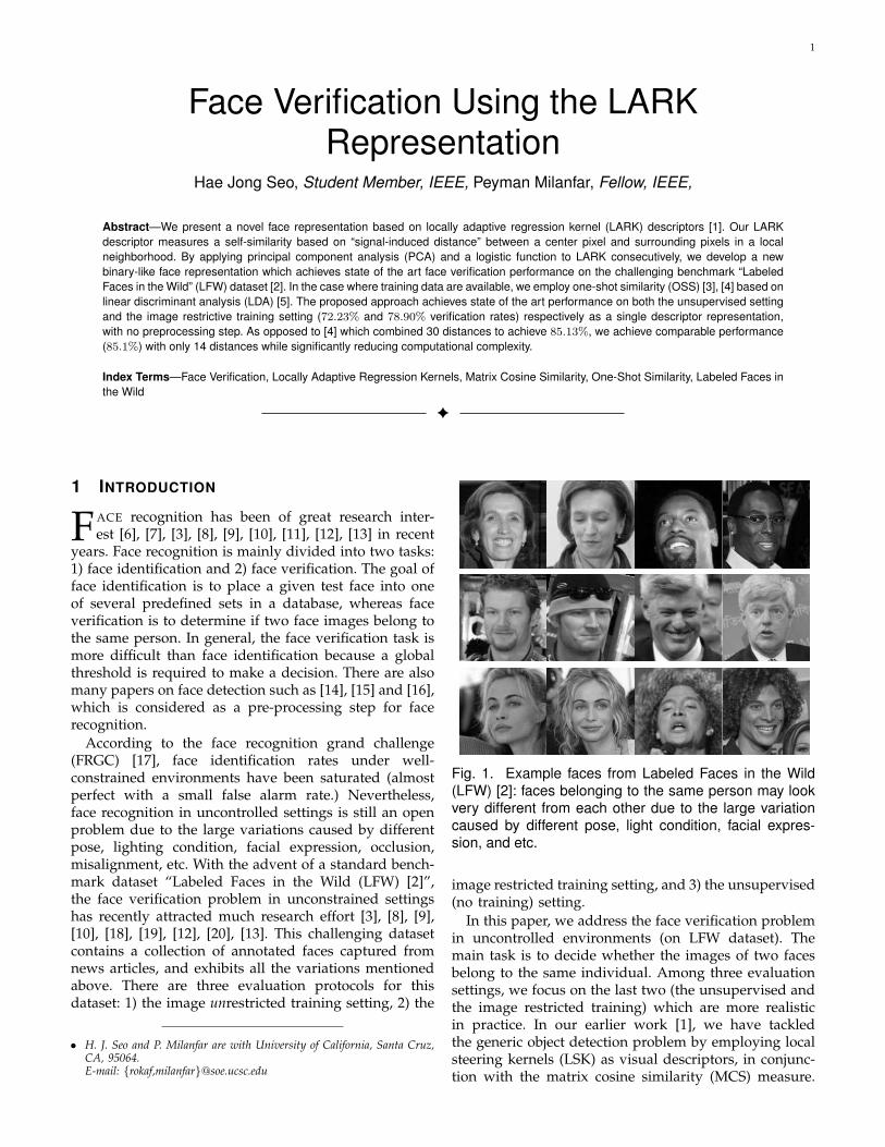
According to the face recognition grand challenge(FRGC) [17], face identification rates under well-constrained environments have been saturated (almostperfect with a small false alarm rate.) Nevertheless,face recognition in uncontrolled settings is still an openproblem due to the large variations caused by differentpose, lighting condition, facial expression, occlusion,misalignment, etc. With the advent of a standard bench-mark dataset “Labeled Faces in the Wild (LFW) [2]”,the face verification problem in unconstrained settingshas recently attracted much research effort [3], [8], [9],[10], [18], [19], [12], [20], [13]. This challenging datasetcontains a collection of annotated faces captured fromnews articles, and exhibits all the variations mentionedabove. There are three evaluation protocols for thisdataset: 1) the image unrestricted training setting, 2) the

• H. J. Seo and P. Milanfar are with University of California, Santa Cruz,CA, 95064.E-mail: rokaf,milanfar@soe.ucsc.edu

Fig. 1. Example faces from Labeled Faces in the Wild(LFW) [2]: faces belonging to the same person may lookvery different from each other due to the large variationcaused by different pose, light condition, facial expres-sion, and etc.

image restricted training setting, and 3) the unsupervised(no training) setting.

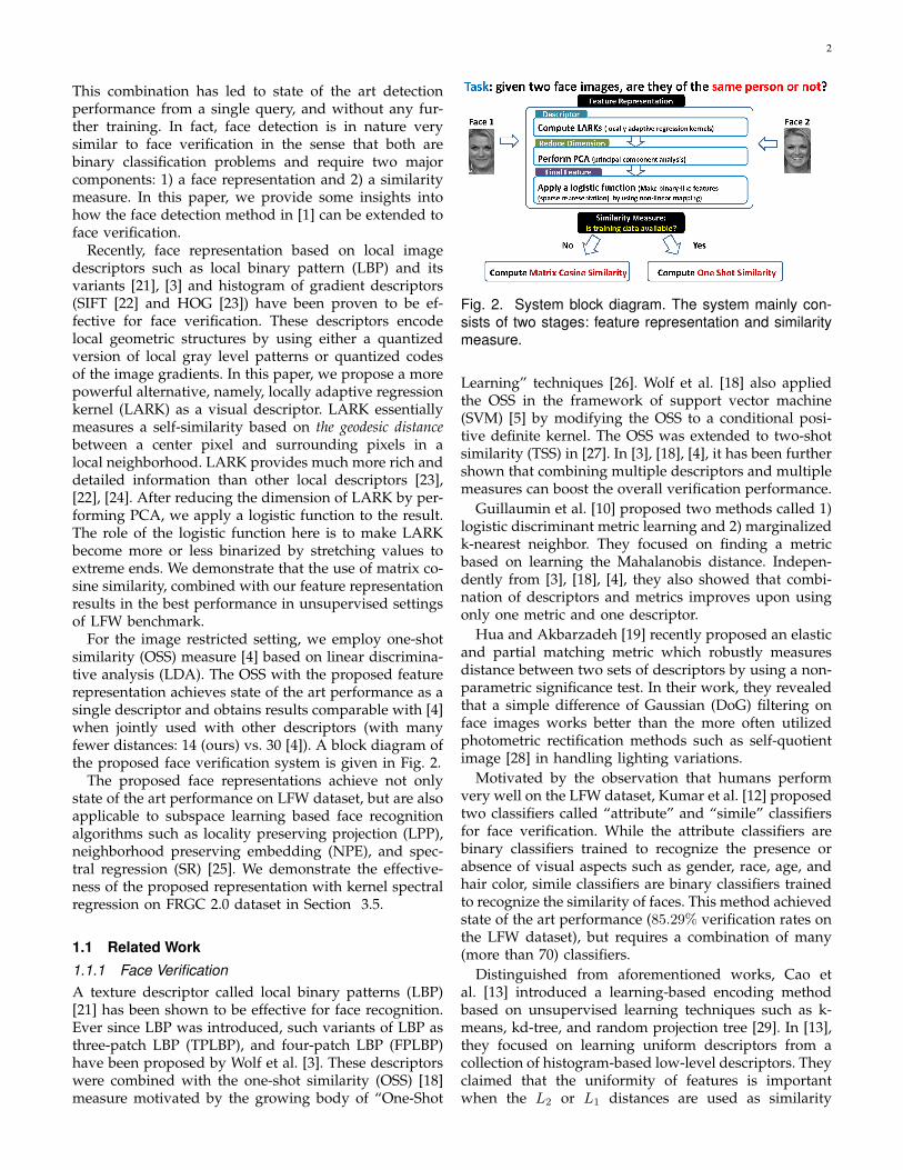
In this paper, we address the face verification problemin uncontrolled environments (on LFW dataset). Themain task is to decide whether the images of two facesbelong to the same individual. Among three evaluationsettings, we focus on the last two (the unsupervised andthe image restricted training) which are more realisticin practice. In our earlier work [1], we have tackledthe generic object detection problem by employing localsteering kernels (LSK) as visual descriptors, in conjunc-tion with the matrix cosine similarity (MCS) measure.

2

This combination has led to state of the art detectionperformance from a single query, and without any fur-ther training. In fact, face detection is in nature verysimilar to face verification in the sense that both arebinary classification problems and require two majorcomponents: 1) a face representation and 2) a similaritymeasure. In this paper, we provide some insights intohow the face detection method in [1] can be extended toface verification.

Recently, face representation based on local imagedescriptors such as local binary pattern (LBP) and itsvariants [21], [3] and histogram of gradient descriptors(SIFT [22] and HOG [23]) have been proven to be ef-fective for face verification. These descriptors encodelocal geometric structures by using either a quantizedversion of local gray level patterns or quantized codesof the image gradients. In this paper, we propose a morepowerful alternative, namely, locally adaptive regressionkernel (LARK) as a visual descriptor. LARK essentiallymeasures a self-similarity based on the geodesic distancebetween a center pixel and surrounding pixels in alocal neighborhood. LARK provides much more rich anddetailed information than other local descriptors [23],[22], [24]. After reducing the dimension of LARK by per-forming PCA, we apply a logistic function to the result.The role of the logistic function here is to make LARKbecome more or less binarized by stretching values toextreme ends. We demonstrate that the use of matrix co-sine similarity, combined with our feature representationresults in the best performance in unsupervised settingsof LFW benchmark.

For the image restricted setting, we employ one-shotsimilarity (OSS) measure [4] based on linear discrimina-tive analysis (LDA). The OSS with the proposed featurerepresentation achieves state of the art performance as asingle descriptor and obtains results comparable with [4]when jointly used with other descriptors (with manyfewer distances: 14 (ours) vs. 30 [4]). A block diagram ofthe proposed face verification system is given in Fig. 2.

The proposed face representations achieve not onlystate of the art performance on LFW dataset, but are alsoapplicable to subspace learning based face recognitionalgorithms such as locality preserving projection (LPP),neighborhood preserving embedding (NPE), and spec-tral regression (SR) [25]. We demonstrate the effective-ness of the proposed representation with kernel spectralregression on FRGC 2.0 dataset in Section 3.5.

1.1 Related Work1.1.1 Face VerificationA texture descriptor called local binary patterns (LBP)[21] has been shown to be effective for face recognition.Ever since LBP was introduced, such variants of LBP asthree-patch LBP (TPLBP), and four-patch LBP (FPLBP)have been proposed by Wolf et al. [3]. These descriptorswere combined with the one-shot similarity (OSS) [18]measure motivated by the growing body of “One-Shot

Fig. 2. System block diagram. The system mainly con-sists of two stages: feature representation and similaritymeasure.

Learning” techniques [26]. Wolf et al. [18] also appliedthe OSS in the framework of support vector machine(SVM) [5] by modifying the OSS to a conditional posi-tive definite kernel. The OSS was extended to two-shotsimilarity (TSS) in [27]. In [3], [18], [4], it has been furthershown that combining multiple descriptors and multiplemeasures can boost the overall verification performance.

Guillaumin et al. [10] proposed two methods called 1)logistic discriminant metric learning and 2) marginalizedk-nearest neighbor. They focused on finding a metricbased on learning the Mahalanobis distance. Indepen-dently from [3], [18], [4], they also showed that combi-nation of descriptors and metrics improves upon usingonly one metric and one descriptor.

Hua and Akbarzadeh [19] recently proposed an elasticand partial matching metric which robustly measuresdistance between two sets of descriptors by using a non-parametric significance test. In their work, they revealedthat a simple difference of Gaussian (DoG) filtering onface images works better than the more often utilizedphotometric rectification methods such as self-quotientimage [28] in handling lighting variations.

Motivated by the observation that humans performvery well on the LFW dataset, Kumar et al. [12] proposedtwo classifiers called “attribute” and “simile” classifiersfor face verification. While the attribute classifiers arebinary classifiers trained to recognize the presence orabsence of visual aspects such as gender, race, age, andhair color, simile classifiers are binary classifiers trainedto recognize the similarity of faces. This method achievedstate of the art performance (85.29% verification rates onthe LFW dataset), but requires a combination of many(more than 70) classifiers.

Distinguished from aforementioned works, Cao etal. [13] introduced a learning-based encoding methodbased on unsupervised learning techniques such as k-means, kd-tree, and random projection tree [29]. In [13],they focused on learning uniform descriptors from acollection of histogram-based low-level descriptors. Theyclaimed that the uniformity of features is importantwhen the L2 or L1 distances are used as similarity

3

spatial

Gray-level

Euclidean distance

Geodesic distance

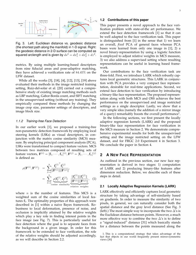
Fig. 3. Left: Euclidean distance vs. geodesic distance(the shortest path along the manifold) in 1-D signal. Right:the geodesic distance in 2-D surface can be computed assquared arclength and is given by ds2 = dx2

1 + dx22 + dz2.

metrics. By using multiple learning-based descriptorsfrom nine fiducial areas and pose-adaptive matching,they have achieved a verification rate of 84.45% on theLFW dataset.

While all the works [3], [18], [4], [12], [13], [19] aboveevaluated their methods in the image restricted trainingsetting, Ruiz-del-solar et al. [20] carried out a compre-hensive study of existing image matching methods suchas LBP matching, Gabor-Borda count, and SIFT matchingin the unsupervised setting (without any training). Theyempirically compared these methods by changing theimage crop size, parameter settings of descriptors, andimage block size.

1.1.2 Training-free Face Detection

In our earlier work [1], we proposed a training-freenon-parametric detection framework by employing localsteering kernels (LSKs) as visual descriptors, in con-junction with the matrix cosine similarity (MCS) mea-sure. By employing principal component analysis (PCA),LSKs were transformed to compact feature vectors. MCSbetween two matrices composed of resulting sets offeature vectors, F(i) = [f1, · · · , fn](i),F(j) = [f1, · · · , fn](j)is defined as:

ρ(F(i),F(j)) =

n∑ℓ=1

f(i)ℓ

⊤f(j)ℓ

∥F(i)∥∥F(j)∥,

=n∑

ℓ=1

ρ(f(i)ℓ , f

(j)ℓ )︸ ︷︷ ︸

cosine similarity

∥f (i)ℓ ∥∥f (j)ℓ ∥∥F(i)∥∥F(j)∥︸ ︷︷ ︸relative weights

, (1)

where n is the number of features. This MCS is aweighted sum of the cosine similarities of local fea-tures fℓ. The optimality properties of this approach weredescribed in [1] within a naive Bayes framework. Ro-bustness to local deformation, presence of noise, andocclusion is implicitly attained by the relative weightswhich play a key role in finding interest points in theface image (see Fig. 7). This is particularly useful forface detection where the goal is to separate faces fromthe background in a given image. In order for thisframework to be extended to face verification, the roleof the relative weights should be adjusted accordingly,as we will describe in Section 2.2.

1.2 Contributions of this paper

This paper presents a novel approach to the face veri-fication problem with state-of-the art performance. Weextend the face detection framework [1] so that it canbe well adapted to the face verification task. This paperis distinguished from [1] in the sense that 1) we learnan overall, fixed PCA of general faces whereas PCAbases were learned from only one image in [1], 2) anovel binary-representation by using a logistic functionis employed to adjust relative weights in MCS measure,3) we also address a supervised setting where resultingrepresentations can be useful in learning based frame-work.

Our contributions to the face verification task arethree-fold. First, we introduce LARK which robustly cap-tures local geometric structures. This LARK in conjunc-tion with PCA provides a very compact face represen-tation, desirable for real-time applications. Second, weextend face detection to face verification by introducinga binary-like face representation. The proposed represen-tation along with both MCS and OSS achieves the bestperformance on the unsupervised and image restrictedsettings as a single descriptor. Lastly, we show that avery simple idea (namely the addition of a mirror imageof a query) remarkably boosts the overall performance1.

In the following sections, we first present the locallyadaptive regression kernels (LARK) and the proposedbinary-like face representation for face verification inthe MCS measure in Section 2. We demonstrate compre-hensive experimental results for both the unsupervisedsetting and the image restricted setting on the LFWdataset, and for FRGC 2.0 Experiment 4 in Section 3.We conclude the paper in Section 4.

2 A NEW FACE REPRESENTATION

As outlined in the previous section, our new face rep-resentation is derived in two stages: 1) computationof LARK and 2) producing binary-like features afterdimension reduction. Below, we describe each of thesesteps in detail.

2.1 Locally Adaptive Regression Kernels (LARK)

LARK effectively and efficiently captures local geometricstructure by taking advantage of self-similarity basedon gradients. In order to measure the similarity of twopixels, in general, we can naturally consider both thespatial distance and the gray level distance (See Fig. 3(left).) The most simple way to incorporate the two ∆’s isthe Euclidean distance between points. However, a muchmore effective way to combine the two ∆’s is to definea “signal-induced” distance [31] which basically standsfor a distance between the points measured along the

1. This is a computational strategy that takes advantage of thefact that objects in our world frequently present mirror-symmetricviews [30]

4

Geodesic distances between LARK values(a center) and surroundings

Gray level patch

at centered at

distance feature similarity feature

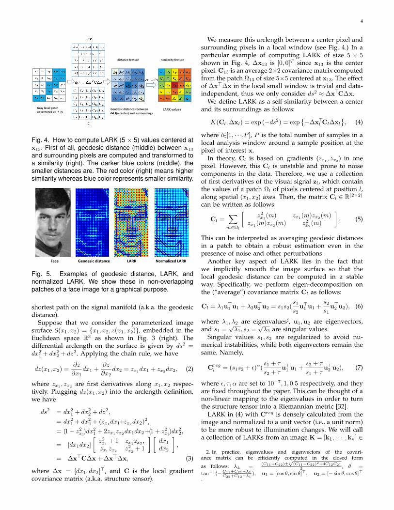
Fig. 4. How to compute LARK (5 × 5) values centered atx13. First of all, geodesic distance (middle) between x13

and surrounding pixels are computed and transformed toa similarity (right). The darker blue colors (middle), thesmaller distances are. The red color (right) means highersimilarity whereas blue color represents smaller similarity.

Face LARK Normalized LARKGeodesic distance

Fig. 5. Examples of geodesic distance, LARK, andnormalized LARK. We show these in non-overlappingpatches of a face image for a graphical purpose.

shortest path on the signal manifold (a.k.a. the geodesicdistance).

Suppose that we consider the parameterized imagesurface S(x1, x2) = x1, x2, z(x1, x2), embedded in theEuclidean space R3 as shown in Fig. 3 (right). Thedifferential arclength on the surface is given by ds2 =dx2

1 + dx22 + dz2. Applying the chain rule, we have

dz(x1, x2) =∂z

∂x1dx1 +

∂z

∂x2dx2 = zx1dx1 + zx2dx2, (2)

where zx1 , zx2 are first derivatives along x1, x2 respec-tively. Plugging dz(x1, x2) into the arclength definition,we have

ds2 = dx21 + dx2

2 + dz2,

= dx21 + dx2

2 + (zx1dx1+zx2dx2)2,

= (1 + z2x1)dx2

1 + 2zx1zx2dx1dx2+(1 + z2x2)dx2

2,

= [dx1dx2]

[z2x1

+ 1 zx1zx2 ,zx1zx2 z2x2

+ 1

] [dx1

dx2

],

= ∆x⊤C∆x+∆x⊤∆x, (3)

where ∆x = [dx1, dx2]⊤, and C is the local gradient

covariance matrix (a.k.a. structure tensor).

We measure this arclength between a center pixel andsurrounding pixels in a local window (see Fig. 4.) In aparticular example of computing LARK of size 5 × 5shown in Fig. 4, ∆x13 is [0, 0]T since x13 is the centerpixel. C13 is an average 2×2 covariance matrix computedfrom the patch Ω13 of size 5×5 centered at x13. The effectof ∆x⊤∆x in the local small window is trivial and data-independent, thus we only consider ds2 ≈ ∆x⊤C∆x.

We define LARK as a self-similarity between a centerand its surroundings as follows:

K(Cl,∆xl) = exp (−ds2) = exp−∆x⊤

l Cl∆xl

, (4)

where l∈[1, · · ·,P ], P is the total number of samples in alocal analysis window around a sample position at thepixel of interest x.

In theory, Cl is based on gradients (zx1 , zx2) in onepixel. However, this Cl is unstable and prone to noisecomponents in the data. Therefore, we use a collectionof first derivatives of the visual signal zl, which containthe values of a patch Ωl of pixels centered at position l,along spatial (x1, x2) axes. Then, the matrix Cl ∈ R(2×2)

can be written as follows:

Cl =∑m∈Ωl

[z2x1

(m) zx1(m)zx2(m)zx1(m)zx2(m) z2x2

(m)

]. (5)

This can be interpreted as averaging geodesic distancesin a patch to obtain a robust estimation even in thepresence of noise and other perturbations.

Another key aspect of LARK lies in the fact thatwe implicitly smooth the image surface so that thelocal geodesic distance can be computed in a stableway. Specifically, we perform eigen-decomposition onthe (“average”) covariance matrix Cl as follows:

Cl = λ1u⊤1 u1 + λ2u

⊤2 u2 = s1s2(

s1s2

u⊤1 u1 +

s2s1

u⊤2 u2), (6)

where λ1, λ2 are eigenvalues2, u1,u2 are eigenvectors,and s1 =

√λ1, s2 =

√λ2 are singular values.

Singular values s1, s2 are regularized to avoid nu-merical instabilities, while both eigenvectors remain thesame. Namely,

Cregl = (s1s2 + ϵ)α(

s1 + τ

s2 + τu⊤1 u1 +

s2 + τ

s1 + τu⊤2 u2), (7)

where ϵ, τ, α are set to 10−7, 1, 0.5 respectively, and theyare fixed throughout the paper. This can be thought of anon-linear mapping to the eigenvalues in order to turnthe structure tensor into a Riemannian metric [32].

LARK in (4) with Creg is densely calculated from theimage and normalized to a unit vector (i.e., a unit norm)to be more robust to illumination changes. We will calla collection of LARKs from an image K = [k1, · · · ,kn] ∈

2. In practice, eigenvalues and eigenvectors of the covari-ance matrix can be efficiently computed in the closed form

as follows: λ± =(C11+C22)±

√(C11−C22)2+4C12C21

2, θ =

tan−1(−C11+C21−λ1C22+C12−λ1

), u1 = [cos θ, sin θ]⊤, u2 = [− sin θ, cos θ]⊤

.

5

Normalized LARK from 120 faces

PCATop 8 eigenvectors (descending order) (90% of energy)

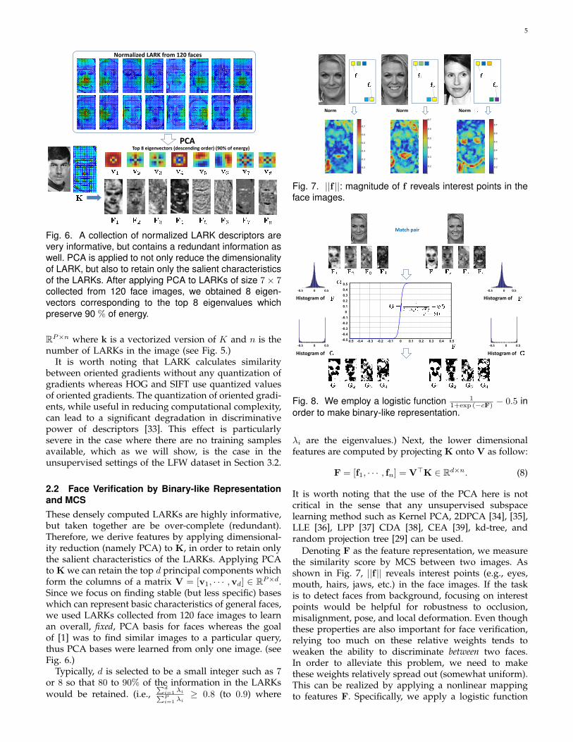
Fig. 6. A collection of normalized LARK descriptors arevery informative, but contains a redundant information aswell. PCA is applied to not only reduce the dimensionalityof LARK, but also to retain only the salient characteristicsof the LARKs. After applying PCA to LARKs of size 7× 7collected from 120 face images, we obtained 8 eigen-vectors corresponding to the top 8 eigenvalues whichpreserve 90 % of energy.

RP×n where k is a vectorized version of K and n is thenumber of LARKs in the image (see Fig. 5.)

It is worth noting that LARK calculates similaritybetween oriented gradients without any quantization ofgradients whereas HOG and SIFT use quantized valuesof oriented gradients. The quantization of oriented gradi-ents, while useful in reducing computational complexity,can lead to a significant degradation in discriminativepower of descriptors [33]. This effect is particularlysevere in the case where there are no training samplesavailable, which as we will show, is the case in theunsupervised settings of the LFW dataset in Section 3.2.

2.2 Face Verification by Binary-like Representationand MCSThese densely computed LARKs are highly informative,but taken together are be over-complete (redundant).Therefore, we derive features by applying dimensional-ity reduction (namely PCA) to K, in order to retain onlythe salient characteristics of the LARKs. Applying PCAto K we can retain the top d principal components whichform the columns of a matrix V = [v1, · · · ,vd] ∈ RP×d.Since we focus on finding stable (but less specific) baseswhich can represent basic characteristics of general faces,we used LARKs collected from 120 face images to learnan overall, fixed, PCA basis for faces whereas the goalof [1] was to find similar images to a particular query,thus PCA bases were learned from only one image. (seeFig. 6.)

Typically, d is selected to be a small integer such as 7or 8 so that 80 to 90% of the information in the LARKswould be retained. (i.e.,

∑di=1 λi∑Pi=1 λi

≥ 0.8 (to 0.9) where

0.2

0.3

0.4

0.5

0.6

0.7

0.2

0.3

0.4

0.5

0.6

0.7

0.2

0.3

0.4

0.5

0.6

0.7

Norm Norm Norm

Fig. 7. ||f ||: magnitude of f reveals interest points in theface images.

-0.5 -0.4 -0.3 -0.2 -0.1 0 0.1 0.2 0.3 0.4 0.5-0.5

-0.4

-0.3

-0.2

-0.1

0

0.1

0.2

0.3

0.4

0.5

Histogram of

Histogram of

Histogram of

Match pair

-0.5 0.50

Histogram of

0.5-0.5 0

-0.5 0.50 -0.5 0.50

Fig. 8. We employ a logistic function 11+exp (−cF) − 0.5 in

order to make binary-like representation.

λi are the eigenvalues.) Next, the lower dimensionalfeatures are computed by projecting K onto V as follow:

F = [f1, · · · , fn] = V⊤K ∈ Rd×n. (8)

It is worth noting that the use of the PCA here is notcritical in the sense that any unsupervised subspacelearning method such as Kernel PCA, 2DPCA [34], [35],LLE [36], LPP [37] CDA [38], CEA [39], kd-tree, andrandom projection tree [29] can be used.

Denoting F as the feature representation, we measurethe similarity score by MCS between two images. Asshown in Fig. 7, ||f || reveals interest points (e.g., eyes,mouth, hairs, jaws, etc.) in the face images. If the taskis to detect faces from background, focusing on interestpoints would be helpful for robustness to occlusion,misalignment, pose, and local deformation. Even thoughthese properties are also important for face verification,relying too much on these relative weights tends toweaken the ability to discriminate between two faces.In order to alleviate this problem, we need to makethese weights relatively spread out (somewhat uniform).This can be realized by applying a nonlinear mappingto features F. Specifically, we apply a logistic function

6

element-by-element to the feature matrices F as follows:

G =1

1 + exp (−cF)− 0.5. (9)

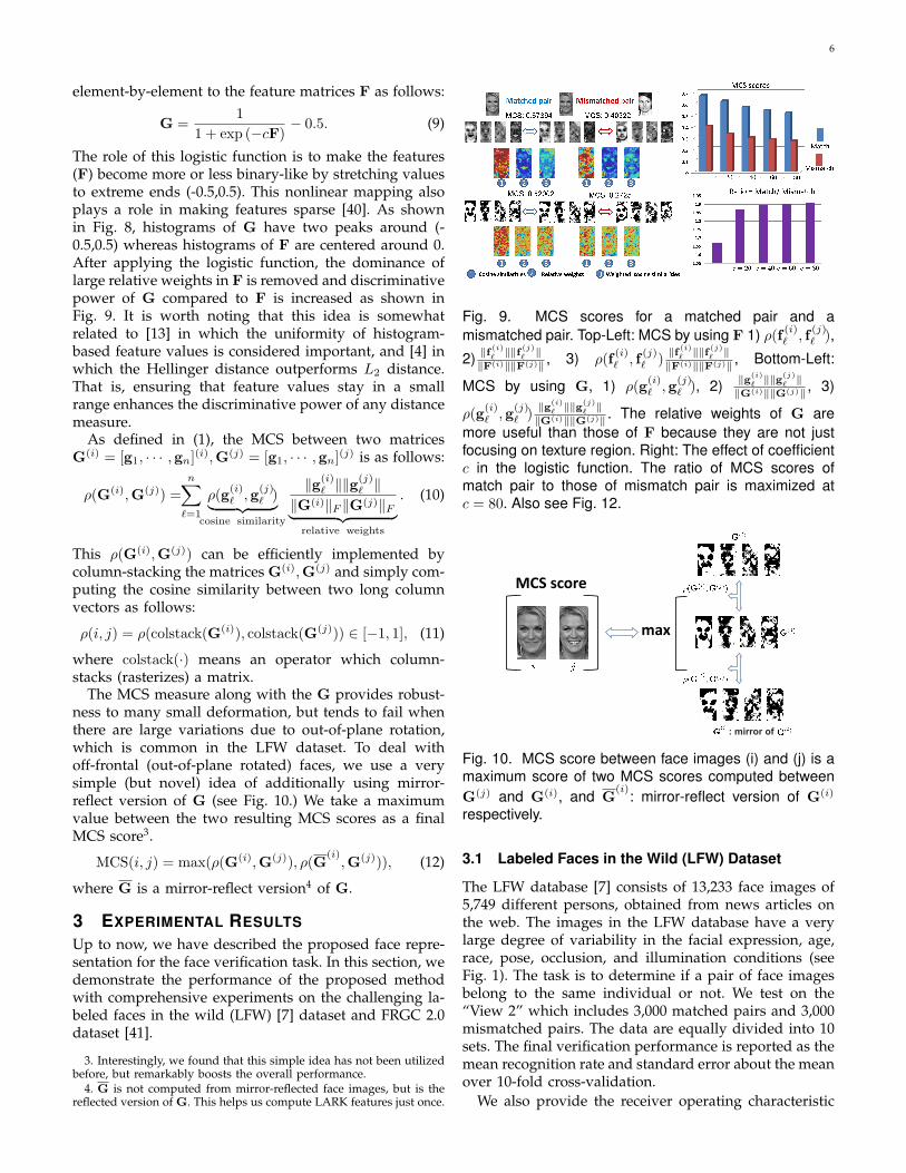
The role of this logistic function is to make the features(F) become more or less binary-like by stretching valuesto extreme ends (-0.5,0.5). This nonlinear mapping alsoplays a role in making features sparse [40]. As shownin Fig. 8, histograms of G have two peaks around (-0.5,0.5) whereas histograms of F are centered around 0.After applying the logistic function, the dominance oflarge relative weights in F is removed and discriminativepower of G compared to F is increased as shown inFig. 9. It is worth noting that this idea is somewhatrelated to [13] in which the uniformity of histogram-based feature values is considered important, and [4] inwhich the Hellinger distance outperforms L2 distance.That is, ensuring that feature values stay in a smallrange enhances the discriminative power of any distancemeasure.

As defined in (1), the MCS between two matricesG(i) = [g1, · · · ,gn]

(i),G(j) = [g1, · · · ,gn](j) is as follows:

ρ(G(i),G(j)) =n∑

ℓ=1

ρ(g(i)ℓ ,g

(j)ℓ )︸ ︷︷ ︸

cosine similarity

∥g(i)ℓ ∥∥g(j)

ℓ ∥∥G(i)∥F ∥G(j)∥F︸ ︷︷ ︸

relative weights

. (10)

This ρ(G(i),G(j)) can be efficiently implemented bycolumn-stacking the matrices G(i),G(j) and simply com-puting the cosine similarity between two long columnvectors as follows:

ρ(i, j) = ρ(colstack(G(i)), colstack(G(j))) ∈ [−1, 1], (11)

where colstack(·) means an operator which column-stacks (rasterizes) a matrix.

The MCS measure along with the G provides robust-ness to many small deformation, but tends to fail whenthere are large variations due to out-of-plane rotation,which is common in the LFW dataset. To deal withoff-frontal (out-of-plane rotated) faces, we use a verysimple (but novel) idea of additionally using mirror-reflect version of G (see Fig. 10.) We take a maximumvalue between the two resulting MCS scores as a finalMCS score3.

MCS(i, j) = max(ρ(G(i),G(j)), ρ(G(i),G(j))), (12)

where G is a mirror-reflect version4 of G.

3 EXPERIMENTAL RESULTSUp to now, we have described the proposed face repre-sentation for the face verification task. In this section, wedemonstrate the performance of the proposed methodwith comprehensive experiments on the challenging la-beled faces in the wild (LFW) [7] dataset and FRGC 2.0dataset [41].

3. Interestingly, we found that this simple idea has not been utilizedbefore, but remarkably boosts the overall performance.

4. G is not computed from mirror-reflected face images, but is thereflected version of G. This helps us compute LARK features just once.

Fig. 9. MCS scores for a matched pair and amismatched pair. Top-Left: MCS by using F 1) ρ(f (i)ℓ , f

(j)ℓ ),

2) ∥f (i)ℓ ∥∥f (j)ℓ ∥∥F(i)∥∥F(j)∥ , 3) ρ(f

(i)ℓ , f

(j)ℓ )

∥f (i)ℓ ∥∥f (j)ℓ ∥∥F(i)∥∥F(j)∥ , Bottom-Left:

MCS by using G, 1) ρ(g(i)ℓ ,g

(j)ℓ ), 2) ∥g(i)

ℓ ∥∥g(j)ℓ ∥

∥G(i)∥∥G(j)∥ , 3)

ρ(g(i)ℓ ,g

(j)ℓ )

∥g(i)ℓ ∥∥g(j)

ℓ ∥∥G(i)∥∥G(j)∥ . The relative weights of G are

more useful than those of F because they are not justfocusing on texture region. Right: The effect of coefficientc in the logistic function. The ratio of MCS scores ofmatch pair to those of mismatch pair is maximized atc = 80. Also see Fig. 12.

max

: mirror of

MCS score

Fig. 10. MCS score between face images (i) and (j) is amaximum score of two MCS scores computed betweenG(j) and G(i), and G

(i): mirror-reflect version of G(i)

respectively.

3.1 Labeled Faces in the Wild (LFW) Dataset

The LFW database [7] consists of 13,233 face images of5,749 different persons, obtained from news articles onthe web. The images in the LFW database have a verylarge degree of variability in the facial expression, age,race, pose, occlusion, and illumination conditions (seeFig. 1). The task is to determine if a pair of face imagesbelong to the same individual or not. We test on the“View 2” which includes 3,000 matched pairs and 3,000mismatched pairs. The data are equally divided into 10sets. The final verification performance is reported as themean recognition rate and standard error about the meanover 10-fold cross-validation.

We also provide the receiver operating characteristic

7

(ROC) curves for the sake of completeness. The truepositive rate (TPR), the false positive rate (FPR), and theverification rate (VR) are defined as follows:

TPR =♯ correctly accepted matched pairs

♯ total matched pairs, (13)

FPR =♯ incorrectly accepted mismatched pairs

♯ total mismatch pairs,(14)

VR =♯ correctly classified pairs

♯ total pairs. (15)

We compute the TPR and FPR by changing the thresholdvalues to draw the ROC curves and report the best VRacross the ROC curves.

As mentioned earlier, there are three evaluation set-tings : 1) the image unrestricted training setting, 2) theimage restricted training setting, and 3) the unsupervisedsetting. The unsupervised setting is the most difficultone among these because there are no training examplesavailable. On the other hand, the other two settings allowus to utilize available image pair information in the train-ing set. The image unrestricted setting further providesthe identity information of each pair. The official LFWwebsite5 provides all the state of the art results on thethree settings.

In this paper, we only focus on the two most chal-lenging settings: the unsupervised setting and the im-age restricted setting, because these scenarios are morerealistic in practice. We use the aligned version of theLFW dataset available from the website6 The imageswere cropped to a size of 184×97 so that images includemore or less faces only7.

3.2 Unsupervised Setting

In this section, we examine the efficacy of the proposedmethod in the unsupervised setting where we do not useany training examples. We compute LARKs (K) of size7 × 7 (based on Ωl of size 7 × 7) densely from eachface image. We end up with features G by reducingdimensionality from 49 to 8 and employing a logisticfunction with c = 80 (performance converges as weincrease c value (see Fig. 9)). The MCS score describedin Fig. 10 is computed from each of 6,000 pairs. [20]conducted comprehensive experiments to find the bestcombination among various state of the art descriptors(i.e., LBP, PCALBP, Gabor jets, and SIFT) and similaritymeasures (i.e, histogram intersection, Chi-square, Bordacount, and Euclidean distance). They reported that LBPwith Chi-square achieves the best performance (69.45%

5. http://vis-www.cs.umass.edu/lfw/results.html6. http://www.openu.ac.il/home/hassner/data/lfwa/ and It is

worth noting that Wolf et al. [4] used a commercial face alignmentsystem based on localization of fiducial points. They reported thatthe aligned version significantly improved the performance of all thedescriptors compared to both the standard and the funneled versions.

7. A slight difference in crop size makes no difference for the overallperformance. For example, consider 184×97 vs. 186×94. More detaileddiscussion about the choice of image crop size in LFW dataset can befound in [42].

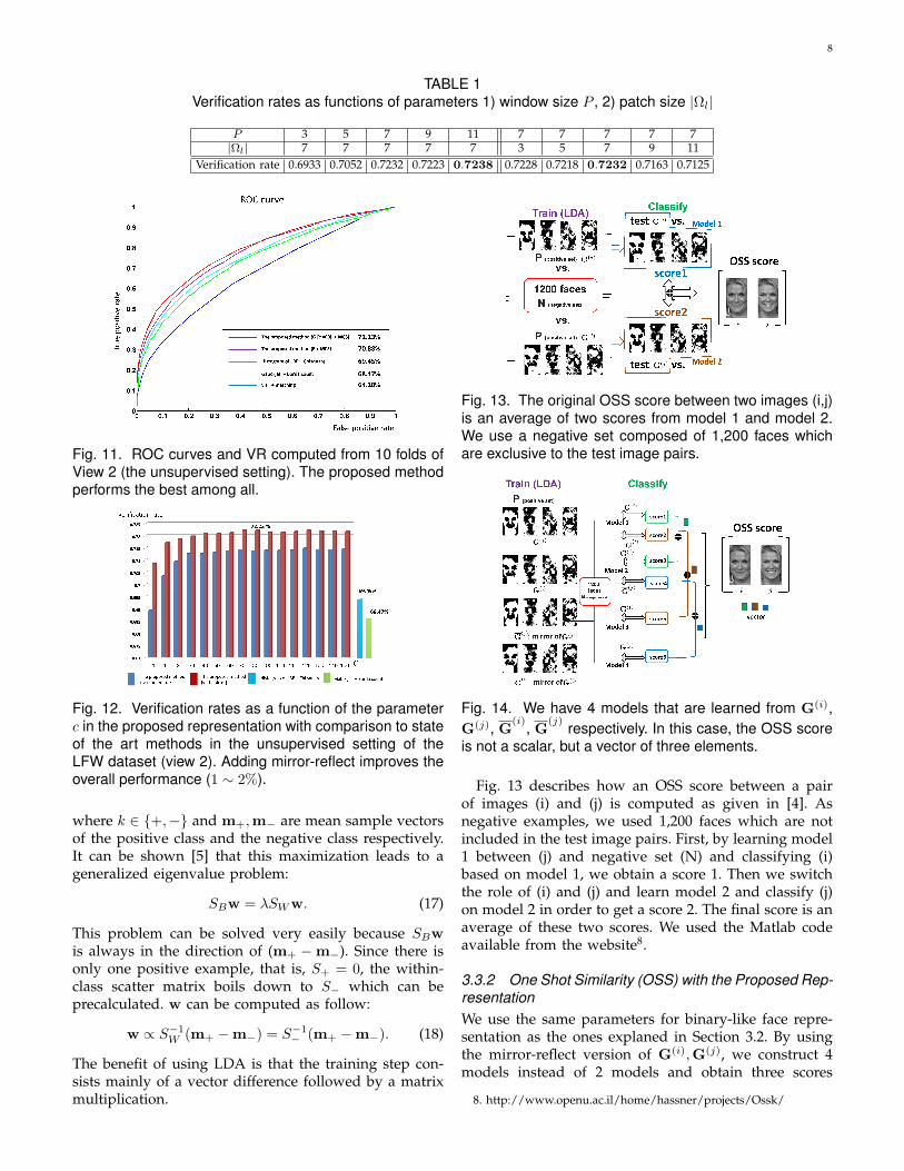
VR). We computed TPR and FPR by changing the thresh-old to draw a ROC curve. The proposed method achieves(72.23% VR) and outperforms previous state of the artmethods reported in the LFW website as shown inFig. 11. Even before employing the logistic function, theproposed approach outperforms state of the art methods.We can see in Fig. 12 that the higher parameter c is,the better performance is. It clearly shows that binary-like features G are superior to the direct use of F forface verification task. We observe that there is no furtherimprovement above c = 80. We also analyzed the effectof using mirror-reflect version of G. This simple idealed to a nontrivial improvement (1 ∼ 2%) which is morepronounced in the range of smaller c. The overall perfor-mance of the proposed method is not a strong functionof 1) LARK window size P and 2) LARK patch size |Ωl|within a desirable range (for instance, P = 7×7 ∼ 11×11)as shown in Table I. If we choose too large a windowsize, the geodesic distance we measure is not accurate.However, if we set the window size to be too small, weend up with insufficient local geometric information. Inother words, local fiducial features such as eye, nose, andmouth will not be captured appropriately. Similarly, thepatch size for computing average covariance matrix Cl

should be set properly. The use of large patch size canover-smooth Cl. Conversely, the use of excessively smallpatch size results in inaccurate estimation of Cl due tonoise. We found that the size of patch Ωl should be lessthan or equal to the window size P .

3.3 Image Restricted SettingIn this section, we deal with the case where there aretraining image pairs available. More specifically, in thetraining set, it is known whether an image pair belongsto the same person or not, while identity information isnot used at all. We employ one-shot similarity (OSS) [4]based on linear discriminative analysis (LDA). We brieflyreview OSS and explain how we use the proposedfeature representation in the OSS framework.

3.3.1 One Shot Similarity (OSS)The key idea behind the OSS is to use negative examples.Suppose that there are two classes (positive (+) andnegative (-)) and we have many negative examples whilethere is only one positive example. In binary LDA case,the goal is to find out a projection direction w whichmaximizes the Raleigh quotient:

w = argmaxw

w⊤SBw

w⊤SWw, (16)

where SB is the “between-class scatter matrix” and SW

is the “within-class scatter matrix.” The definitions of thescatter matrices are as follows:

SB = (m+ −m−)(m+ −m−)⊤,

SW = S+ + S−,

Sk =∑k

(Gk −mk)(Gk −mk)⊤,

8

TABLE 1Verification rates as functions of parameters 1) window size P , 2) patch size |Ωl|

P 3 5 7 9 11 7 7 7 7 7|Ωl| 7 7 7 7 7 3 5 7 9 11

Verification rate 0.6933 0.7052 0.7232 0.7223 0.7238 0.7228 0.7218 0.7232 0.7163 0.7125

Fig. 11. ROC curves and VR computed from 10 folds ofView 2 (the unsupervised setting). The proposed methodperforms the best among all.

Fig. 12. Verification rates as a function of the parameterc in the proposed representation with comparison to stateof the art methods in the unsupervised setting of theLFW dataset (view 2). Adding mirror-reflect improves theoverall performance (1 ∼ 2%).

where k ∈ +,− and m+,m− are mean sample vectorsof the positive class and the negative class respectively.It can be shown [5] that this maximization leads to ageneralized eigenvalue problem:

SBw = λSWw. (17)

This problem can be solved very easily because SBwis always in the direction of (m+ − m−). Since there isonly one positive example, that is, S+ = 0, the within-class scatter matrix boils down to S− which can beprecalculated. w can be computed as follow:

w ∝ S−1W (m+ −m−) = S−1

− (m+ −m−). (18)

The benefit of using LDA is that the training step con-sists mainly of a vector difference followed by a matrixmultiplication.

Fig. 13. The original OSS score between two images (i,j)is an average of two scores from model 1 and model 2.We use a negative set composed of 1,200 faces whichare exclusive to the test image pairs.

Fig. 14. We have 4 models that are learned from G(i),G(j), G

(i), G

(j)respectively. In this case, the OSS score

is not a scalar, but a vector of three elements.

Fig. 13 describes how an OSS score between a pairof images (i) and (j) is computed as given in [4]. Asnegative examples, we used 1,200 faces which are notincluded in the test image pairs. First, by learning model1 between (j) and negative set (N) and classifying (i)based on model 1, we obtain a score 1. Then we switchthe role of (i) and (j) and learn model 2 and classify (j)on model 2 in order to get a score 2. The final score is anaverage of these two scores. We used the Matlab codeavailable from the website8.

3.3.2 One Shot Similarity (OSS) with the Proposed Rep-resentationWe use the same parameters for binary-like face repre-sentation as the ones explaned in Section 3.2. By usingthe mirror-reflect version of G(i),G(j), we construct 4models instead of 2 models and obtain three scores

8. http://www.openu.ac.il/home/hassner/projects/Ossk/

9

TABLE 2Test set, Negative set, and Training sets in 10-fold validation (view 2)

Fold 1 2 3 4 5 6 7 8 9 10Test set 3∼10 1, 4∼10 1,2, 5∼10 1∼3, 6∼10 1∼4, 7∼10 1∼5, 8∼10 1∼6, 9∼10 1∼7, 10 1∼8 2∼9

Negative set 2 3 4 5 6 7 8 9 10 1Train set 1 2 3 4 5 6 7 8 9 10

TABLE 3Mean verification rates (10-fold) on the LFW dataset (view 2) . sqrt means

√descriptors which is Hellinger distance

and Mirror means that mirror-reflect version is added.

Descriptors L2 distance L2 + sqrt MCS MCS + sqrt OSS OSS+ sqrtLBP 67.86% 68.53% 67.98% 68.18% 74.48% 74.41%

LBP (Mirror) 68.33% 69.08% 71.0% 67.61% 75.65% 76.05%TPLBP 68.28% 68.78% 68.35% 67.76% 74.7% 74.58%

TPLBP (Mirror) 68.98% 69.38% 71.66% 68.6% 77.08% 76.1%SIFT 71.01% 71.05% 70.65% 70.96% 73.13% 76.4%

SIFT (Mirror) 71.3% 71.08% 71.26% 71.3% 73.2% 78.2%L2 distance L2 + logistic(c=80) MCS MCS + logistic(c=80) OSS OSS+ logistic(c=80)

Ours 65.81% 70.98% 68.25% 71.08% 75.81% 76.45%Ours (Mirror) 66.28% 73.23% 71.26% 73.3% 76.38% 78.9%

TABLE 4Mean verification rates (10-fold) on the LFW dataset (view 2) . standard set VS. aligned set

Dataset standard aligned standard aligned

Descriptor MCS + logistic(c=80) MCS + logistic(c=80) OSS+ logistic(c=80) OSS+ logistic(c=80)Ours 66.65% 71.08% 70.97% 76.45%

Ours (Mirror) 68.35% 73.3% 71.96% 78.9%

TABLE 5Mean verification rate (10-fold) comparison between [4] and our best result. TSS means the two shot similarity [4].

Numbers mean the number of descriptors used.

Method L2 L2 + sqrt TSS TSS + sqrt OSS OSS + sqrtWolf et al. [4] LBP, Gabor LBP, Gabor LBP, Gabor LBP, Gabor LBP, Gabor, LBP, Gabor

(30) FPLBP, TPLBP FPLBP, TPLBP FPLBP, TPLBP FPLBP, TPLBP FPLBP, TPLBP FPLBP, TPLBP85.13 ±0.37% SIFT (5) SIFT (5) SIFT (5) SIFT (5) SIFT (5) SIFT (5)

Method L2 distance L2 + logistic(c=80) MCS MCS + logistic(c=80) OSS OSS+ logistic(c=80)Ours (14) TPLBP (3) TPLBP (3) LBP, TPLBP LBP, TPLBP

85.10 ±0.59% (0) (0) SIFT, pcaLARK SIFT, pcaLARK SIFT, pcaLARK (4) SIFT, pcaLARK (4)

0 0.01 0.02 0.03 0.04 0.05 0.06 0.07 0.08 0.09 0.10

0.1

0.2

0.3

0.4

0.5

0.6

0.7

0.8

0.9

False positive rate

Tru

e p

osi

tive

ra

te

ROC curve

Wolf et al. (ACCV ‘09) (60 distances)

Cao et al. (multi) (CVPR ‘10)

Kumar et al. (ICCV ‘09)

Cao et al. (single) (CVPR ‘10)

The proposed

[OSS (8) + MCS(6) = (14 distances) ]

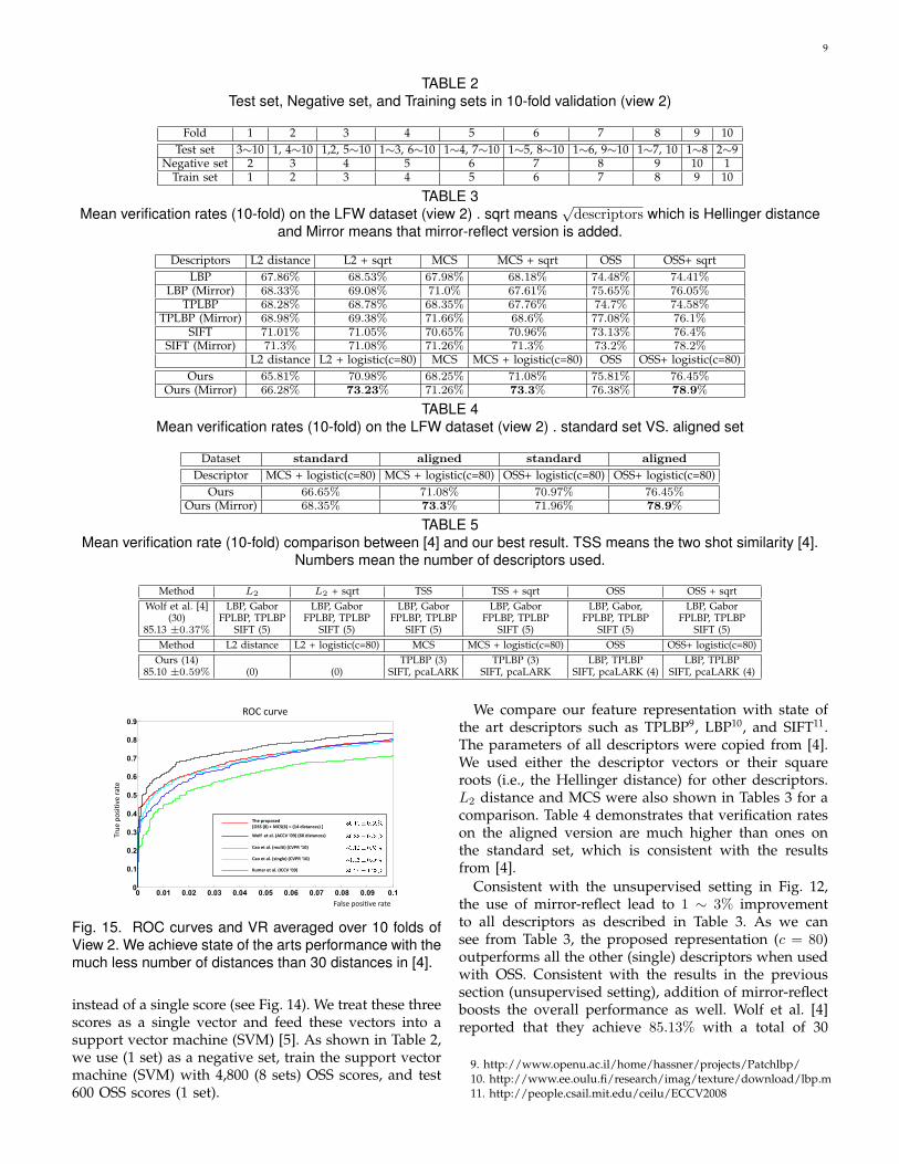
Fig. 15. ROC curves and VR averaged over 10 folds ofView 2. We achieve state of the arts performance with themuch less number of distances than 30 distances in [4].

instead of a single score (see Fig. 14). We treat these threescores as a single vector and feed these vectors into asupport vector machine (SVM) [5]. As shown in Table 2,we use (1 set) as a negative set, train the support vectormachine (SVM) with 4,800 (8 sets) OSS scores, and test600 OSS scores (1 set).

We compare our feature representation with state ofthe art descriptors such as TPLBP9, LBP10, and SIFT11.The parameters of all descriptors were copied from [4].We used either the descriptor vectors or their squareroots (i.e., the Hellinger distance) for other descriptors.L2 distance and MCS were also shown in Tables 3 for acomparison. Table 4 demonstrates that verification rateson the aligned version are much higher than ones onthe standard set, which is consistent with the resultsfrom [4].

Consistent with the unsupervised setting in Fig. 12,the use of mirror-reflect lead to 1 ∼ 3% improvementto all descriptors as described in Table 3. As we cansee from Table 3, the proposed representation (c = 80)outperforms all the other (single) descriptors when usedwith OSS. Consistent with the results in the previoussection (unsupervised setting), addition of mirror-reflectboosts the overall performance as well. Wolf et al. [4]reported that they achieve 85.13% with a total of 30

9. http://www.openu.ac.il/home/hassner/projects/Patchlbp/10. http://www.ee.oulu.fi/research/imag/texture/download/lbp.m11. http://people.csail.mit.edu/ceilu/ECCV2008

10

query target

Cropped images in our experiment Cropped images in [44]

query target

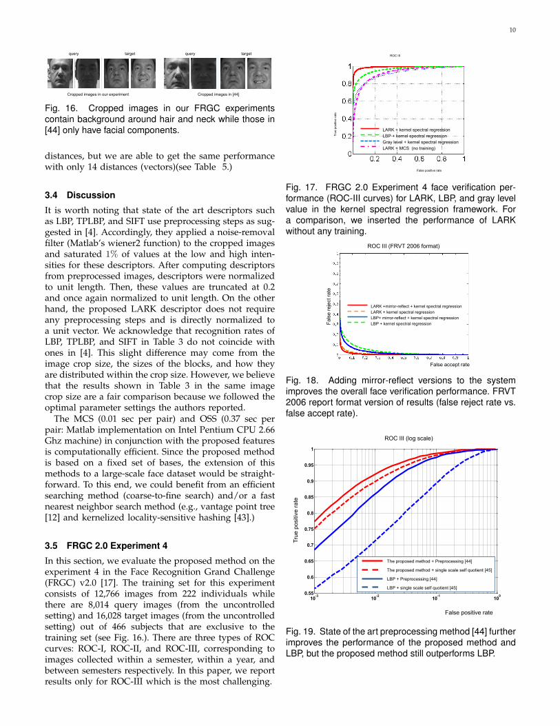
Fig. 16. Cropped images in our FRGC experimentscontain background around hair and neck while those in[44] only have facial components.

distances, but we are able to get the same performancewith only 14 distances (vectors)(see Table 5.)

3.4 Discussion

It is worth noting that state of the art descriptors suchas LBP, TPLBP, and SIFT use preprocessing steps as sug-gested in [4]. Accordingly, they applied a noise-removalfilter (Matlab’s wiener2 function) to the cropped imagesand saturated 1% of values at the low and high inten-sities for these descriptors. After computing descriptorsfrom preprocessed images, descriptors were normalizedto unit length. Then, these values are truncated at 0.2and once again normalized to unit length. On the otherhand, the proposed LARK descriptor does not requireany preprocessing steps and is directly normalized toa unit vector. We acknowledge that recognition rates ofLBP, TPLBP, and SIFT in Table 3 do not coincide withones in [4]. This slight difference may come from theimage crop size, the sizes of the blocks, and how theyare distributed within the crop size. However, we believethat the results shown in Table 3 in the same imagecrop size are a fair comparison because we followed theoptimal parameter settings the authors reported.

The MCS (0.01 sec per pair) and OSS (0.37 sec perpair: Matlab implementation on Intel Pentium CPU 2.66Ghz machine) in conjunction with the proposed featuresis computationally efficient. Since the proposed methodis based on a fixed set of bases, the extension of thismethods to a large-scale face dataset would be straight-forward. To this end, we could benefit from an efficientsearching method (coarse-to-fine search) and/or a fastnearest neighbor search method (e.g., vantage point tree[12] and kernelized locality-sensitive hashing [43].)

3.5 FRGC 2.0 Experiment 4

In this section, we evaluate the proposed method on theexperiment 4 in the Face Recognition Grand Challenge(FRGC) v2.0 [17]. The training set for this experimentconsists of 12,766 images from 222 individuals whilethere are 8,014 query images (from the uncontrolledsetting) and 16,028 target images (from the uncontrolledsetting) out of 466 subjects that are exclusive to thetraining set (see Fig. 16.). There are three types of ROCcurves: ROC-I, ROC-II, and ROC-III, corresponding toimages collected within a semester, within a year, andbetween semesters respectively. In this paper, we reportresults only for ROC-III which is the most challenging.

Tru

e p

ositiv

e r

ate

False positive rate

ROC III

LARK + kernel spectral regression

LBP + kernel spectral regression

LARK + MCS (no training)

Gray level + kernel spectral regression

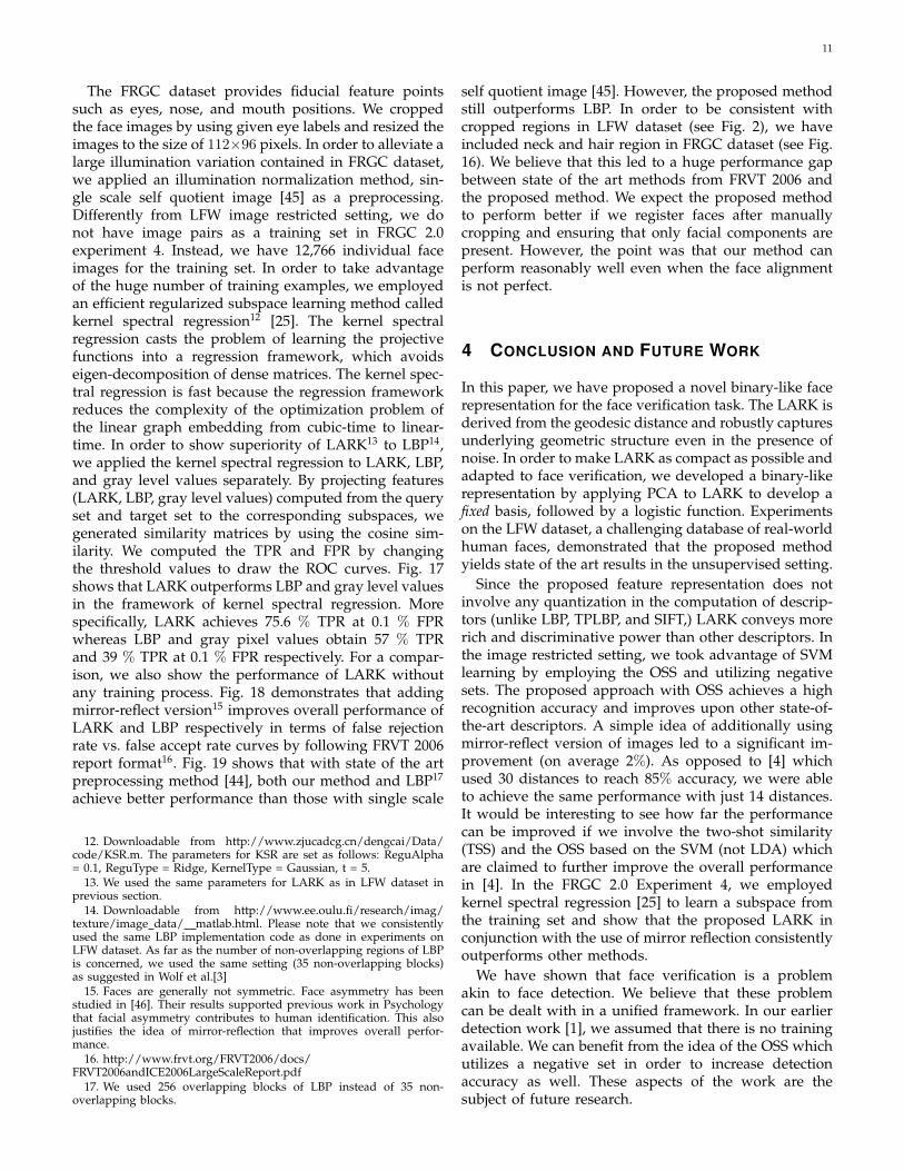
Fig. 17. FRGC 2.0 Experiment 4 face verification per-formance (ROC-III curves) for LARK, LBP, and gray levelvalue in the kernel spectral regression framework. Fora comparison, we inserted the performance of LARKwithout any training.

Fals

e r

eje

ct ra

te

False accept rate

ROC III (FRVT 2006 format)

LARK +mirror-reflect + kernel spectral regression

LARK + kernel spectral regression

LBP + kernel spectral regression

LBP+ mirror-reflect + kernel spectral regression

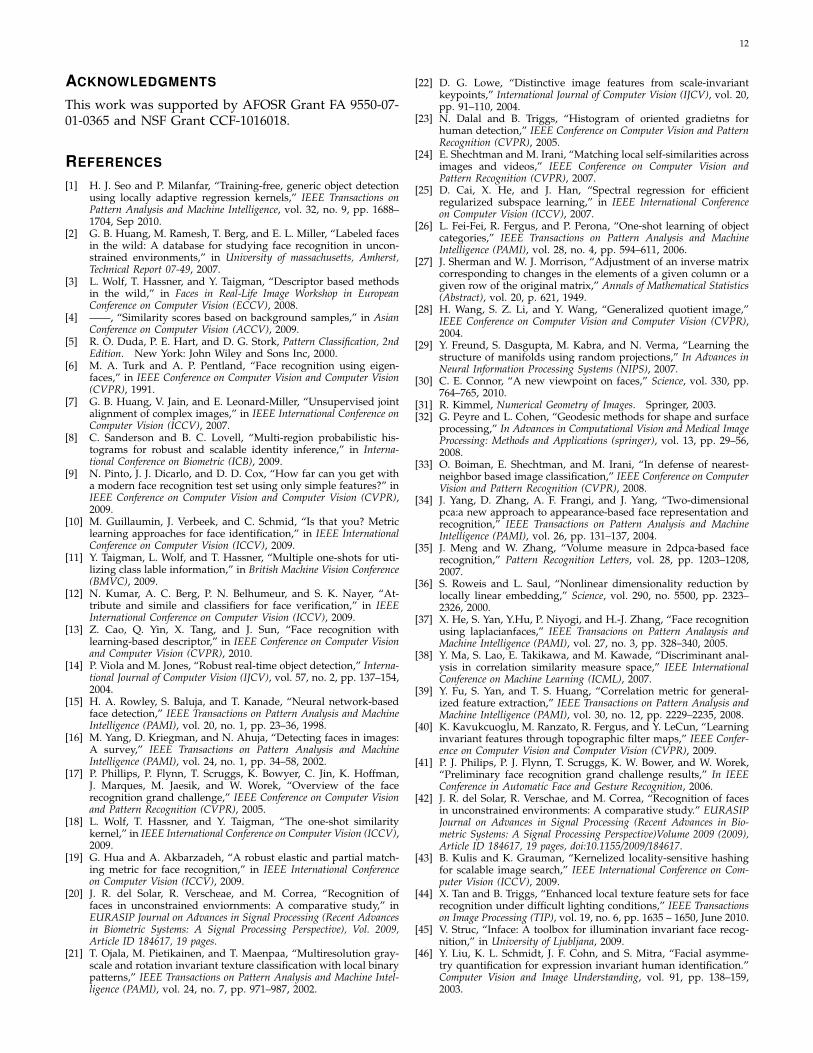
Fig. 18. Adding mirror-reflect versions to the systemimproves the overall face verification performance. FRVT2006 report format version of results (false reject rate vs.false accept rate).

10-3

10-2

10-1

100

0.55

0.6

0.65

0.7

0.75

0.8

0.85

0.9

0.95

1

Tru

e p

ositiv

e r

ate

False positive rate

ROC III (log scale)

The proposed method + Preprocessing [44]

The proposed method + single scale self quotient [45]

LBP + single scale self quotient [45]

LBP + Preprocessing [44]

Fig. 19. State of the art preprocessing method [44] furtherimproves the performance of the proposed method andLBP, but the proposed method still outperforms LBP.

11

The FRGC dataset provides fiducial feature pointssuch as eyes, nose, and mouth positions. We croppedthe face images by using given eye labels and resized theimages to the size of 112×96 pixels. In order to alleviate alarge illumination variation contained in FRGC dataset,we applied an illumination normalization method, sin-gle scale self quotient image [45] as a preprocessing.Differently from LFW image restricted setting, we donot have image pairs as a training set in FRGC 2.0experiment 4. Instead, we have 12,766 individual faceimages for the training set. In order to take advantageof the huge number of training examples, we employedan efficient regularized subspace learning method calledkernel spectral regression12 [25]. The kernel spectralregression casts the problem of learning the projectivefunctions into a regression framework, which avoidseigen-decomposition of dense matrices. The kernel spec-tral regression is fast because the regression frameworkreduces the complexity of the optimization problem ofthe linear graph embedding from cubic-time to linear-time. In order to show superiority of LARK13 to LBP14,we applied the kernel spectral regression to LARK, LBP,and gray level values separately. By projecting features(LARK, LBP, gray level values) computed from the queryset and target set to the corresponding subspaces, wegenerated similarity matrices by using the cosine sim-ilarity. We computed the TPR and FPR by changingthe threshold values to draw the ROC curves. Fig. 17shows that LARK outperforms LBP and gray level valuesin the framework of kernel spectral regression. Morespecifically, LARK achieves 75.6 % TPR at 0.1 % FPRwhereas LBP and gray pixel values obtain 57 % TPRand 39 % TPR at 0.1 % FPR respectively. For a compar-ison, we also show the performance of LARK withoutany training process. Fig. 18 demonstrates that addingmirror-reflect version15 improves overall performance ofLARK and LBP respectively in terms of false rejectionrate vs. false accept rate curves by following FRVT 2006report format16. Fig. 19 shows that with state of the artpreprocessing method [44], both our method and LBP17

achieve better performance than those with single scale

12. Downloadable from http://www.zjucadcg.cn/dengcai/Data/code/KSR.m. The parameters for KSR are set as follows: ReguAlpha= 0.1, ReguType = Ridge, KernelType = Gaussian, t = 5.

13. We used the same parameters for LARK as in LFW dataset inprevious section.

14. Downloadable from http://www.ee.oulu.fi/research/imag/texture/image data/ matlab.html. Please note that we consistentlyused the same LBP implementation code as done in experiments onLFW dataset. As far as the number of non-overlapping regions of LBPis concerned, we used the same setting (35 non-overlapping blocks)as suggested in Wolf et al.[3]

15. Faces are generally not symmetric. Face asymmetry has beenstudied in [46]. Their results supported previous work in Psychologythat facial asymmetry contributes to human identification. This alsojustifies the idea of mirror-reflection that improves overall perfor-mance.

16. http://www.frvt.org/FRVT2006/docs/FRVT2006andICE2006LargeScaleReport.pdf

17. We used 256 overlapping blocks of LBP instead of 35 non-overlapping blocks.

self quotient image [45]. However, the proposed methodstill outperforms LBP. In order to be consistent withcropped regions in LFW dataset (see Fig. 2), we haveincluded neck and hair region in FRGC dataset (see Fig.16). We believe that this led to a huge performance gapbetween state of the art methods from FRVT 2006 andthe proposed method. We expect the proposed methodto perform better if we register faces after manuallycropping and ensuring that only facial components arepresent. However, the point was that our method canperform reasonably well even when the face alignmentis not perfect.

4 CONCLUSION AND FUTURE WORK

In this paper, we have proposed a novel binary-like facerepresentation for the face verification task. The LARK isderived from the geodesic distance and robustly capturesunderlying geometric structure even in the presence ofnoise. In order to make LARK as compact as possible andadapted to face verification, we developed a binary-likerepresentation by applying PCA to LARK to develop afixed basis, followed by a logistic function. Experimentson the LFW dataset, a challenging database of real-worldhuman faces, demonstrated that the proposed methodyields state of the art results in the unsupervised setting.

Since the proposed feature representation does notinvolve any quantization in the computation of descrip-tors (unlike LBP, TPLBP, and SIFT,) LARK conveys morerich and discriminative power than other descriptors. Inthe image restricted setting, we took advantage of SVMlearning by employing the OSS and utilizing negativesets. The proposed approach with OSS achieves a highrecognition accuracy and improves upon other state-of-the-art descriptors. A simple idea of additionally usingmirror-reflect version of images led to a significant im-provement (on average 2%). As opposed to [4] whichused 30 distances to reach 85% accuracy, we were ableto achieve the same performance with just 14 distances.It would be interesting to see how far the performancecan be improved if we involve the two-shot similarity(TSS) and the OSS based on the SVM (not LDA) whichare claimed to further improve the overall performancein [4]. In the FRGC 2.0 Experiment 4, we employedkernel spectral regression [25] to learn a subspace fromthe training set and show that the proposed LARK inconjunction with the use of mirror reflection consistentlyoutperforms other methods.

We have shown that face verification is a problemakin to face detection. We believe that these problemcan be dealt with in a unified framework. In our earlierdetection work [1], we assumed that there is no trainingavailable. We can benefit from the idea of the OSS whichutilizes a negative set in order to increase detectionaccuracy as well. These aspects of the work are thesubject of future research.

12

ACKNOWLEDGMENTS

This work was supported by AFOSR Grant FA 9550-07-01-0365 and NSF Grant CCF-1016018.

REFERENCES

[1] H. J. Seo and P. Milanfar, “Training-free, generic object detectionusing locally adaptive regression kernels,” IEEE Transactions onPattern Analysis and Machine Intelligence, vol. 32, no. 9, pp. 1688–1704, Sep 2010.

[2] G. B. Huang, M. Ramesh, T. Berg, and E. L. Miller, “Labeled facesin the wild: A database for studying face recognition in uncon-strained environments,” in University of massachusetts, Amherst,Technical Report 07-49, 2007.

[3] L. Wolf, T. Hassner, and Y. Taigman, “Descriptor based methodsin the wild,” in Faces in Real-Life Image Workshop in EuropeanConference on Computer Vision (ECCV), 2008.

[4] ——, “Similarity scores based on background samples,” in AsianConference on Computer Vision (ACCV), 2009.

[5] R. O. Duda, P. E. Hart, and D. G. Stork, Pattern Classification, 2ndEdition. New York: John Wiley and Sons Inc, 2000.

[6] M. A. Turk and A. P. Pentland, “Face recognition using eigen-faces,” in IEEE Conference on Computer Vision and Computer Vision(CVPR), 1991.

[7] G. B. Huang, V. Jain, and E. Leonard-Miller, “Unsupervised jointalignment of complex images,” in IEEE International Conference onComputer Vision (ICCV), 2007.

[8] C. Sanderson and B. C. Lovell, “Multi-region probabilistic his-tograms for robust and scalable identity inference,” in Interna-tional Conference on Biometric (ICB), 2009.

[9] N. Pinto, J. J. Dicarlo, and D. D. Cox, “How far can you get witha modern face recognition test set using only simple features?” inIEEE Conference on Computer Vision and Computer Vision (CVPR),2009.

[10] M. Guillaumin, J. Verbeek, and C. Schmid, “Is that you? Metriclearning approaches for face identification,” in IEEE InternationalConference on Computer Vision (ICCV), 2009.

[11] Y. Taigman, L. Wolf, and T. Hassner, “Multiple one-shots for uti-lizing class lable information,” in British Machine Vision Conference(BMVC), 2009.

[12] N. Kumar, A. C. Berg, P. N. Belhumeur, and S. K. Nayer, “At-tribute and simile and classifiers for face verification,” in IEEEInternational Conference on Computer Vision (ICCV), 2009.

[13] Z. Cao, Q. Yin, X. Tang, and J. Sun, “Face recognition withlearning-based descriptor,” in IEEE Conference on Computer Visionand Computer Vision (CVPR), 2010.

[14] P. Viola and M. Jones, “Robust real-time object detection,” Interna-tional Journal of Computer Vision (IJCV), vol. 57, no. 2, pp. 137–154,2004.

[15] H. A. Rowley, S. Baluja, and T. Kanade, “Neural network-basedface detection,” IEEE Transactions on Pattern Analysis and MachineIntelligence (PAMI), vol. 20, no. 1, pp. 23–36, 1998.

[16] M. Yang, D. Kriegman, and N. Ahuja, “Detecting faces in images:A survey,” IEEE Transactions on Pattern Analysis and MachineIntelligence (PAMI), vol. 24, no. 1, pp. 34–58, 2002.

[17] P. Phillips, P. Flynn, T. Scruggs, K. Bowyer, C. Jin, K. Hoffman,J. Marques, M. Jaesik, and W. Worek, “Overview of the facerecognition grand challenge,” IEEE Conference on Computer Visionand Pattern Recognition (CVPR), 2005.

[18] L. Wolf, T. Hassner, and Y. Taigman, “The one-shot similaritykernel,” in IEEE International Conference on Computer Vision (ICCV),2009.

[19] G. Hua and A. Akbarzadeh, “A robust elastic and partial match-ing metric for face recognition,” in IEEE International Conferenceon Computer Vision (ICCV), 2009.

[20] J. R. del Solar, R. Verscheae, and M. Correa, “Recognition offaces in unconstrained enviornments: A comparative study,” inEURASIP Journal on Advances in Signal Processing (Recent Advancesin Biometric Systems: A Signal Processing Perspective), Vol. 2009,Article ID 184617, 19 pages.

[21] T. Ojala, M. Pietikainen, and T. Maenpaa, “Multiresolution gray-scale and rotation invariant texture classification with local binarypatterns,” IEEE Transactions on Pattern Analysis and Machine Intel-ligence (PAMI), vol. 24, no. 7, pp. 971–987, 2002.

[22] D. G. Lowe, “Distinctive image features from scale-invariantkeypoints,” International Journal of Computer Vision (IJCV), vol. 20,pp. 91–110, 2004.

[23] N. Dalal and B. Triggs, “Histogram of oriented gradietns forhuman detection,” IEEE Conference on Computer Vision and PatternRecognition (CVPR), 2005.

[24] E. Shechtman and M. Irani, “Matching local self-similarities acrossimages and videos,” IEEE Conference on Computer Vision andPattern Recognition (CVPR), 2007.

[25] D. Cai, X. He, and J. Han, “Spectral regression for efficientregularized subspace learning,” in IEEE International Conferenceon Computer Vision (ICCV), 2007.

[26] L. Fei-Fei, R. Fergus, and P. Perona, “One-shot learning of objectcategories,” IEEE Transactions on Pattern Analysis and MachineIntelligence (PAMI), vol. 28, no. 4, pp. 594–611, 2006.

[27] J. Sherman and W. J. Morrison, “Adjustment of an inverse matrixcorresponding to changes in the elements of a given column or agiven row of the original matrix,” Annals of Mathematical Statistics(Abstract), vol. 20, p. 621, 1949.

[28] H. Wang, S. Z. Li, and Y. Wang, “Generalized quotient image,”IEEE Conference on Computer Vision and Computer Vision (CVPR),2004.

[29] Y. Freund, S. Dasgupta, M. Kabra, and N. Verma, “Learning thestructure of manifolds using random projections,” In Advances inNeural Information Processing Systems (NIPS), 2007.

[30] C. E. Connor, “A new viewpoint on faces,” Science, vol. 330, pp.764–765, 2010.

[31] R. Kimmel, Numerical Geometry of Images. Springer, 2003.[32] G. Peyre and L. Cohen, “Geodesic methods for shape and surface

processing,” In Advances in Computational Vision and Medical ImageProcessing: Methods and Applications (springer), vol. 13, pp. 29–56,2008.

[33] O. Boiman, E. Shechtman, and M. Irani, “In defense of nearest-neighbor based image classification,” IEEE Conference on ComputerVision and Pattern Recognition (CVPR), 2008.

[34] J. Yang, D. Zhang, A. F. Frangi, and J. Yang, “Two-dimensionalpca:a new approach to appearance-based face representation andrecognition,” IEEE Transactions on Pattern Analysis and MachineIntelligence (PAMI), vol. 26, pp. 131–137, 2004.

[35] J. Meng and W. Zhang, “Volume measure in 2dpca-based facerecognition,” Pattern Recognition Letters, vol. 28, pp. 1203–1208,2007.

[36] S. Roweis and L. Saul, “Nonlinear dimensionality reduction bylocally linear embedding,” Science, vol. 290, no. 5500, pp. 2323–2326, 2000.

[37] X. He, S. Yan, Y.Hu, P. Niyogi, and H.-J. Zhang, “Face recognitionusing laplacianfaces,” IEEE Transacions on Pattern Analaysis andMachine Intelligence (PAMI), vol. 27, no. 3, pp. 328–340, 2005.

[38] Y. Ma, S. Lao, E. Takikawa, and M. Kawade, “Discriminant anal-ysis in correlation similarity measure space,” IEEE InternationalConference on Machine Learning (ICML), 2007.

[39] Y. Fu, S. Yan, and T. S. Huang, “Correlation metric for general-ized feature extraction,” IEEE Transactions on Pattern Analysis andMachine Intelligence (PAMI), vol. 30, no. 12, pp. 2229–2235, 2008.

[40] K. Kavukcuoglu, M. Ranzato, R. Fergus, and Y. LeCun, “Learninginvariant features through topographic filter maps,” IEEE Confer-ence on Computer Vision and Computer Vision (CVPR), 2009.

[41] P. J. Philips, P. J. Flynn, T. Scruggs, K. W. Bower, and W. Worek,“Preliminary face recognition grand challenge results,” In IEEEConference in Automatic Face and Gesture Recognition, 2006.

[42] J. R. del Solar, R. Verschae, and M. Correa, “Recognition of facesin unconstrained environments: A comparative study.” EURASIPJournal on Advances in Signal Processing (Recent Advances in Bio-metric Systems: A Signal Processing Perspective)Volume 2009 (2009),Article ID 184617, 19 pages, doi:10.1155/2009/184617.

[43] B. Kulis and K. Grauman, “Kernelized locality-sensitive hashingfor scalable image search,” IEEE International Conference on Com-puter Vision (ICCV), 2009.

[44] X. Tan and B. Triggs, “Enhanced local texture feature sets for facerecognition under difficult lighting conditions,” IEEE Transactionson Image Processing (TIP), vol. 19, no. 6, pp. 1635 – 1650, June 2010.

[45] V. Struc, “Inface: A toolbox for illumination invariant face recog-nition,” in University of Ljubljana, 2009.

[46] Y. Liu, K. L. Schmidt, J. F. Cohn, and S. Mitra, “Facial asymme-try quantification for expression invariant human identification.”Computer Vision and Image Understanding, vol. 91, pp. 138–159,2003.