1

Facility Layout

Creating a New Layout

To create a new layout, select the New Layout Option from the Facility Layout

menu. The dialog box below is presented. Provide the Name of the project, the

number of departments, number of fixed points and the distance measure. When the

Make Random Problem box is checked, random interdepartmental flows are provided.

We will discuss the purpose of the fixed point parameter on page 23.

Pressing OK results in the Layout Data worksheet shown below. The data for the

example is already filled in. The user should enter the facility length and width

measured in the specified distance measure (meters in this case). The distance

measure is converted into cells using

the scale factor. The program limits

the maximum facility dimensions to

50 cells wide by 100 cells long. When

one of the specified plant dimension

exceeds the limit, a scale factor greater

than 1 must be entered to convert the

distance measure to a cell measure. A

scale factor greater than 1 reduces the

size of the facility and results in

quicker solution times.

Cells colored yellow should not be

changed. They contain either

formulas or quantities fixed by the

program. The name defining the problem is reflected in the worksheet name and the

named ranges on the worksheet so the name in cell B2 should not be changed. The

number of departments is also fixed. The data cells with white backgrounds can be

changed.

2

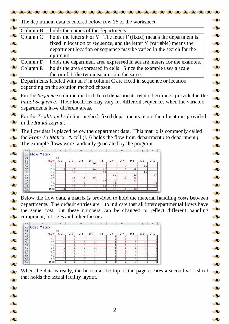
The department data is entered below row 16 of the worksheet.

Column B holds the names of the departments.

Column C holds the letters F or V. The letter F (fixed) means the department is

fixed in location or sequence, and the letter V (variable) means the

department location or sequence may be varied in the search for the

optimum.

Column D holds the department area expressed in square meters for the example.

Column E holds the area expressed in cells. Since the example uses a scale

factor of 1, the two measures are the same.

Departments labeled with an F in column C are fixed in sequence or location

depending on the solution method chosen.

For the Sequence solution method, fixed departments retain their index provided in the

Initial Sequence. Their locations may vary for different sequences when the variable

departments have different areas.

For the Traditional solution method, fixed departments retain their locations provided

in the Initial Layout.

The flow data is placed below the department data. This matrix is commonly called

the From-To Matrix. A cell (i, j) holds the flow from department i to department j.

The example flows were randomly generated by the program.

Below the flow data, a matrix is provided to hold the material handling costs between

departments. The default entries are 1 to indicate that all interdepartmental flows have

the same cost, but these numbers can be changed to reflect different handling

equipment, lot sizes and other factors.

When the data is ready, the button at the top of the page creates a second worksheet

that holds the actual facility layout.

3

Defining the Facility

The button on the Layout Data worksheet presents the dialog box

shown below with which the various solution options are selected.

The distance between two departments is the distance between their respective

centroids. When material movement is parallel to the length and width boundaries of

the plant, it is reasonable to use the Rectilinear measure. When the movement is via

straight lines between the two centroids, the Euclidean measure is appropriate.

Two solution options are available, the Optimum Sequence method and the Traditional

Craft. The length and width of the plant and the aisle width are set in the fields at the

bottom.

The facility layout worksheet has various parameters and options listed at the top of

the page as illustrated below.

At the top of the page in column B we see the name, number of departments, length

and width of the facility, total area and the cost for the current layout. We hope to find

a layout that minimizes the cost in cell B8. Column E holds parameters that are

described subsequently.

Starting in row 11, a row is provided for each department.

Column A holds the department name

column B holds its color

column C holds the area defined on the Layout Data worksheet

column D holds the area defined for the department on the current layout

Columns E and F hold the computed centroids of the department. For this example,

we are using an Aisle layout.

Column G shows the sequence number of the department.

The ranges shown in green hold numbers computed by the program.

Width

Len

gth

4

When the Sequential button is selected for the initial solution, a layout is automatically

generated with the departments listed in numerical order in column G. This is the

default initial sequence, but the numbers in this column can be changed to

accommodate a user-supplied initial sequence. This is important if some departments

are given a fixed index in the sequence.

The Leave Blank option is available only with traditional craft. Here the layout is left

blank initially and the user must manually define the department locations in the

layout. The layout is immediately to the right of this data on the worksheet.

The initial layout for the example was generated with the default sequence using an

Aisle layout and is shown below.

5

The layout starts in cell J11. The number of colored cells to the right of J11 is the

width of the facility and the number of colored cells below J11 is its length. The

locations of the departments are specified by department indices or colors. The initial

layout can be entered manually or automatically. It is most convenient to use an

automatic Aisle layout. The aisles are indicated by the white lines running through the

centers of the departments.

The aisle layout is determined by the department width, which for the example is

equal to 5, and the sequence of departments. For the example, we have chosen the

sequence as the department indices. The first department in the sequence starts in cell

J11 and is assigned cells to the right until the department area is completely defined or

the department width is reached. For the example, department 1 requires all five cells.

The second department is placed below the first, using as many rows as necessary to

enter the entire area. We continue to add departments until the entire length of the

facility is used. Then the departments are placed at the bottom of aisle 2. In the

example, department 4 uses both aisles 1 and 2. The layout continues up aisle 2 until

the top is reached for department 8. Then the layout proceeds down aisle 3 until all

departments are placed. For the example, five cells remain unused. The white lines

on the layout show the serpentine nature of this layout procedure.

6

Change Facility:

To illustrate the effect of a different department width we click

button. The dialog below is presented. Any of the options may be changed. In this

case, we change the depth to 4.

Because the department areas are not multiples of 4, the layout becomes more

irregular. This affects that accuracy of distance measurements since department

centroids are no longer in the center of rectangular departments.

An alternative layout that more nearly maintains rectangular departments is obtained

when the Full Width box is checked. The result for the example is shown below. For

this option, departments are increased in area so that they fill an integral number of

rows of the layout. Note that the area of department 1 has increased from 5 to 8. Of

course, when department areas are increased, it may be necessary to increase the size

of the facility. This is the case for the example where it is necessary to increase the

length of the facility to 12 so that the larger departments can be accommodated.

The next step is to search for the

optimum layout. We consider

first the Optimum Sequence

method and then the Traditional

Craft method.

7

Optimum Sequence Method

The sequential layout is defined by the department width and the sequence used to

layout the departments along the aisles of the facility. The optimum sequence method

of solution starts with an arbitrary اعتباطي initial sequential solution and tries to improve

the layout by switching two departments in the sequence. At each step, the method

computes the cost changes for all possible switches of two departments and chooses

the most effective pair. The two departments are switched in the sequence and the

method repeats. The process STOPS when no switch results in a reduced cost. To

illustrate we start with the departments sequenced in order of department index as

below.

Clicking the button presents the dialog below.

Starting from the initial sequence, the program finds the best switch and presents its

conclusion below.

8

Clicking Yes causes the change in

layout. Notice that departments 9

and 10 are switched in sequence

and in location.

The next best switch is

departments 1 and 3. Notice that

the change in sequence affects the

relative locations of the

departments switched. When the

departments are of different size,

the locations of all departments

between are also adjusted.

We restarted the process with the

initial sequence and chose the Do

Not Stop option. The process

stopped with no further

improvement after one additional

switch of departments 6 and 7.

The result is shown.

9

To the right of the layout appears a

summary of the switches made during

the process.

Above the layout there are several

additional buttons. The

button generates a random sequence of

departments and places them on the

layout. Since the switch heuristic does

not guarantee optimality, it is useful to

start at several different solutions and

select the best.

The button evaluates the current sequence placed in column G of the

worksheet. The user can manually change the sequence. The button allows

the user to force the program to switch two departments. The button

draws lines between centroids to show the flows.

For the example we generated a random sequence using the button and

performed the switch procedure until no improvement was possible. The resulting

layout is shown below with the summary results. Note that this layout is much

different that the one previously discovered. Its cost is slightly larger than before.

11

We initiated the layout with a

department width of 4 with the

resultant sequential layout as

below.

After a sequence of switches we

obtain the final layout shown with its summary below.

Clicking the button

shows the flow lines between

departmental centroids. The

thickness of a line shows the relative

magnitude of the flow-cost between

two of the departments. Four

different thickness are used with a

thin line indicating a relative small

flow-cost between two departments

and a thick line indicating a large

flow-cost.

The sequential layout can be easily automatically generated. The sequential layout

method quickly finds good layouts for alternative facility designs. The Traditional

Craft method is an alternative.

11

2. Traditional CRAFT Method

To create a worksheet for the Traditional

Craft option, click that button on the Options

dialog . The most convenient way

to initialize the layout is with a sequential

layout. Otherwise, click the Leave Blank

button.

2.1 Sequential Initial Solution

To illustrate the CRAFT method we start with a sequential layout with the

departments sequenced in order of department index as below. The CRAFT method is

not limited to this kind of initial solution, but it is convenient since the process is

automatic.

Similar to the sequential method, the CRAFT method also investigates departments

for switching. Candidates for switching are pairs of departments that have the same

area or pairs of departments that are adjacent in the layout. For example, consider the

feasible switches that involve department 6 in the layout above. Departments 2 and 8

have the same area, so the pairs (2, 6) and (6, 8) are feasible. Departments that are

adjacent to 6 are departments 3, 5, 7, 9 and 10, so the pairs involving these

departments and department 6 are feasible.

To evaluate the effect of switching the two departments, the CRAFT method assumes

that the centroids of the two departments are switched and computes the resultant cost

12

savings. When the two departments are the same size, this evaluation is accurate.

When the departments have different sizes, the centroids of the departments do not

exactly switch locations. In this case the evaluation may be not be accurate and a

switch that looks promising may actually increase the cost of the layout. The CRAFT

method implemented by this add-in terminates if this occurs.

For the example, the best feasible

pair is 9 and 10. Since the two

departments are different sizes,

there are many alternatives for

arranging the cells of the smaller

sized department 9 into the larger

area formerly holding department

10. The program has an algorithm

for choosing the arrangement that

results in the layout below.

Although one might question the

logic of this arrangement, it is

difficult to program an algorithm

that always makes the most reasonable assignment. The user can adjust the

assignment of cells by changing cell indices, but this is a manual operation.

The next iteration interchanges departments 2 and 3.

13

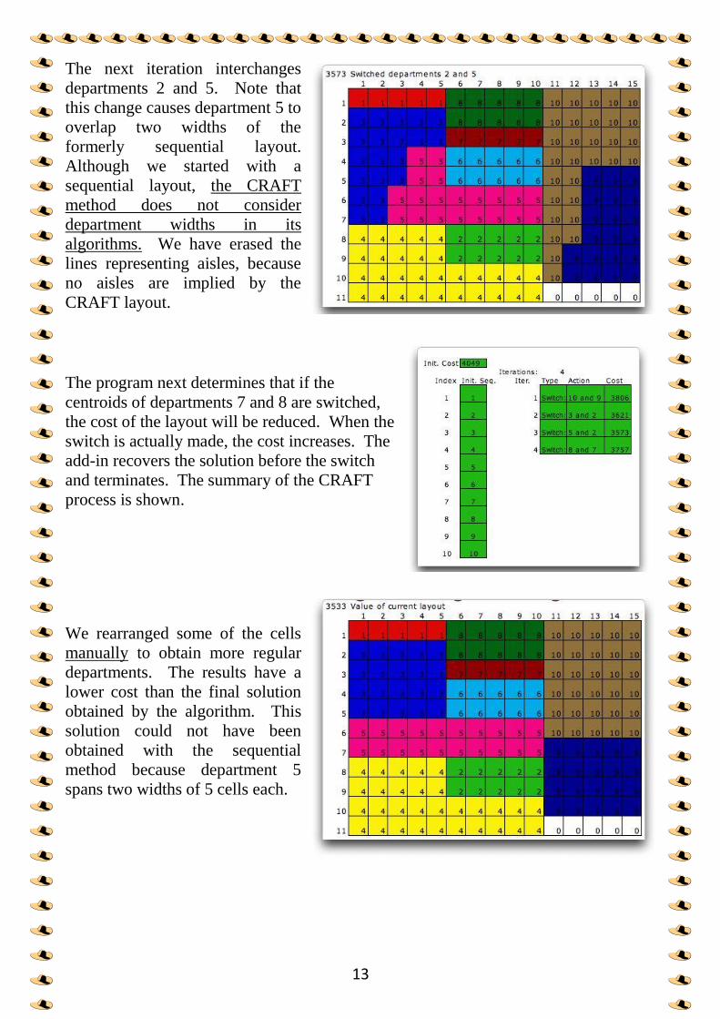
The next iteration interchanges

departments 2 and 5. Note that

this change causes department 5 to

overlap two widths of the

formerly sequential layout.

Although we started with a

sequential layout, the CRAFT

method does not consider

department widths in its

algorithms. We have erased the

lines representing aisles, because

no aisles are implied by the

CRAFT layout.

The program next determines that if the

centroids of departments 7 and 8 are switched,

the cost of the layout will be reduced. When the

switch is actually made, the cost increases. The

add-in recovers the solution before the switch

and terminates. The summary of the CRAFT

process is shown.

We rearranged some of the cells

manually to obtain more regular

departments. The results have a

lower cost than the final solution

obtained by the algorithm. This

solution could not have been

obtained with the sequential

method because department 5

spans two widths of 5 cells each.

14

2.2 Blank Initial Solution

The CRAFT method is not restricted to initial layouts obtained by the sequential

method. By choosing Blank on the dialog, a blank layout is presented.

An initial layout is constructed by placing numbers or colors on the layout. One

possible initial layout is below.

The blank spaces might represent the actual building shape or unusable portions of the

facility. Pressing the Evaluate button, colors the cells and evaluates the layout.

15

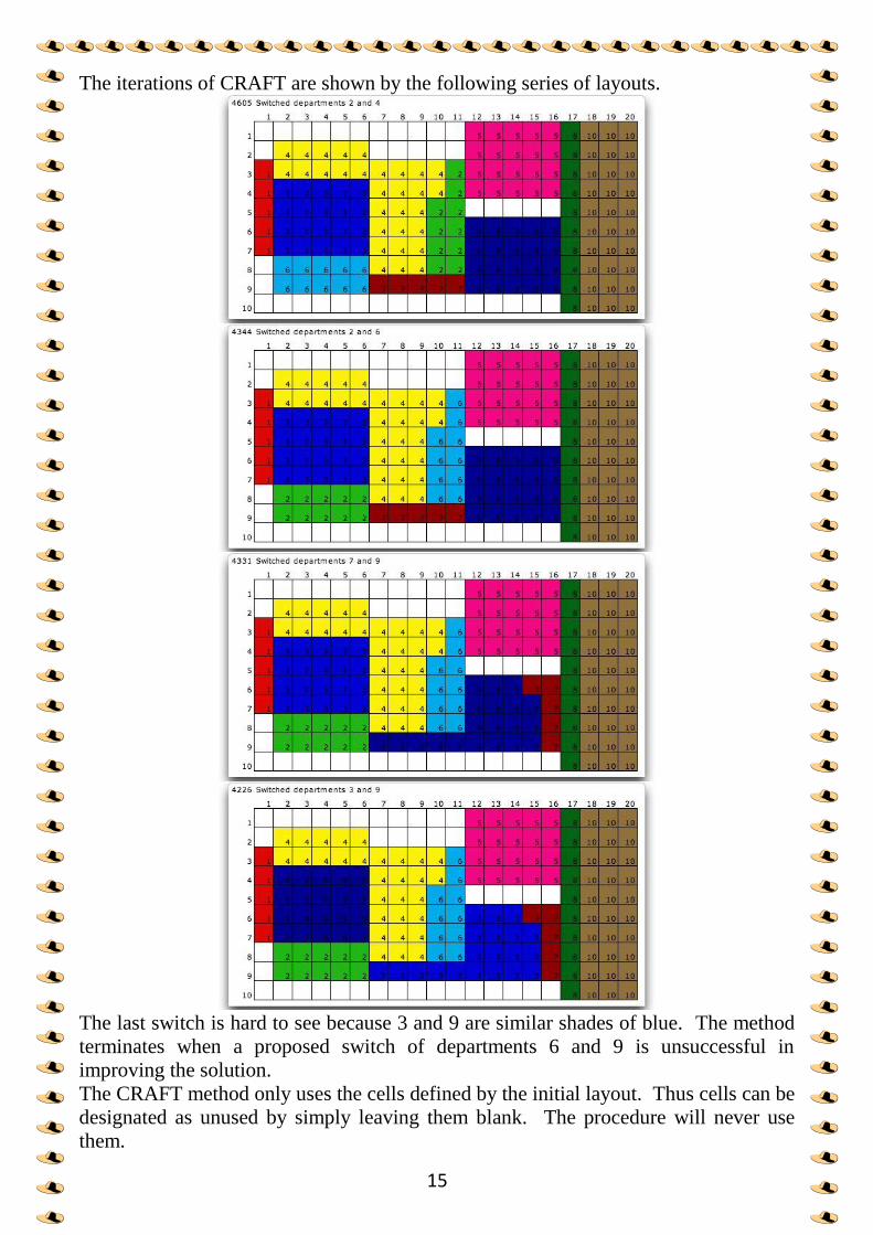
The iterations of CRAFT are shown by the following series of layouts.

The last switch is hard to see because 3 and 9 are similar shades of blue. The method

terminates when a proposed switch of departments 6 and 9 is unsuccessful in

improving the solution.

The CRAFT method only uses the cells defined by the initial layout. Thus cells can be

designated as unused by simply leaving them blank. The procedure will never use

them.

16

Fixed Points

It is often true that department flow also passes to or from fixed points in the facility.

For example, the facility probably includes one or more loading or shipping docks.

Raw materials arrive at some docks while finished goods leave at others. Workers may

travel between departments and fixed points within the facility, such as restrooms or

tool cribs.

We have included five fixed points in the

facility considered previously. The data for the

fixed points appears to the right of the

interdepartmental flow data. The x-proportion

and y-proportion tell where the fixed point is

located relative to the width and length of the

facility. When the proportions are (0, 0), the

point is at the upper-left corner of the facility.

When the proportions are (1, 1), the point is at

the lower-right corner of the facility.

Proportions (0.5, 0.5) places the point in the

center of the facility area. We have entered data

for flows between departments and fixed points

as below.

In diagrams showing the layout, the

fixed points are shown as black dots.

The cost of flow to the fixed points is

considered during the optimization.

The solution for the example is shown

below with the flow-cost lines

superimposed.

As many as 50 fixed points may be

included in the facility.

17

-Layout Buttons

When a workbook is opened on a computer different than the one in which it was

created, the buttons on the worksheets are not linked to the Layout Add-in. Selecting

the Layout Buttons menu items, recreates the buttons and links them to the resident

add-in.

Optimize

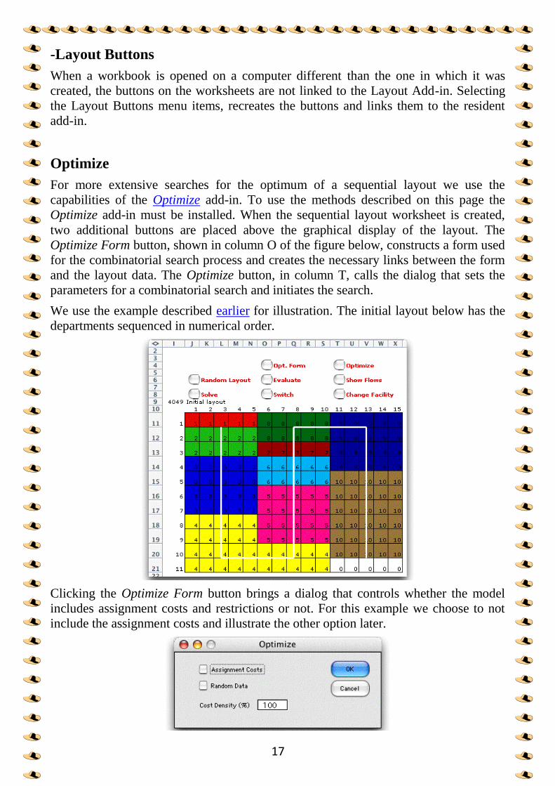
For more extensive searches for the optimum of a sequential layout we use the

capabilities of the Optimize add-in. To use the methods described on this page the

Optimize add-in must be installed. When the sequential layout worksheet is created,

two additional buttons are placed above the graphical display of the layout. The

Optimize Form button, shown in column O of the figure below, constructs a form used

for the combinatorial search process and creates the necessary links between the form

and the layout data. The Optimize button, in column T, calls the dialog that sets the

parameters for a combinatorial search and initiates the search.

We use the example described earlier for illustration. The initial layout below has the

departments sequenced in numerical order.

Clicking the Optimize Form button brings a dialog that controls whether the model

includes assignment costs and restrictions or not. For this example we choose to not

include the assignment costs and illustrate the other option later.

18

Clicking the OK button creates the form shown below at the right of the layout. The

form shows the initial permutation describing the layout. Rows 3 through 5 hold

information used by the search procedure. Cell AL has a link to Cell B8, where the

computed value of the layout is calculated. The range of cells AJ8 through AS8 are

manipulated by the search algorithms. They are linked by Excel formulas to the range

G11 through G20, the cells that define the sequence for the Layout add-in. The cells in

row 10 are constructed by the Optimize add-in but are not used when assignment costs

are not considered. The Feasibility conditions defined by cells AN3 and AN4 are not

used for the example.

Clicking the Optimize button presents the

Search dialog with various options for

searching for the optimum permutation

and the associated layout. For the

illustration we have chosen to randomly

generate 10 permutations or layout

sequences. Notice that the form does not

allow a Greedy solution. We have

disabled this button because the algorithm

of the Optimize add-in used for the greedy

solution of permutations does not work

for the layout application.

The Optimize add-in generates 10 random permutations and the Layout add-in

evaluates them. The best of the 10 are placed on the combinatorial form. The 10

solutions appear to the right of this display (shown below the form on this page).

19

The layout associated with the best of the solutions is shown below. It happens that

this solution is not as good as the initial solution.

We continue in our search for the

optimum by starting from the best

random result and choosing the

improvement option that tries all 2

and 3-change variations of the

layout. The process first tries all

2-change variations and whenever

a change results an improvement,

the two permutation positions are

switched in value. The process

continues until no 2-change

switch results in improvement,

then all 3-change switches are

evaluated. The program

terminates when a complete run

through the changes results in no

improvement.

21

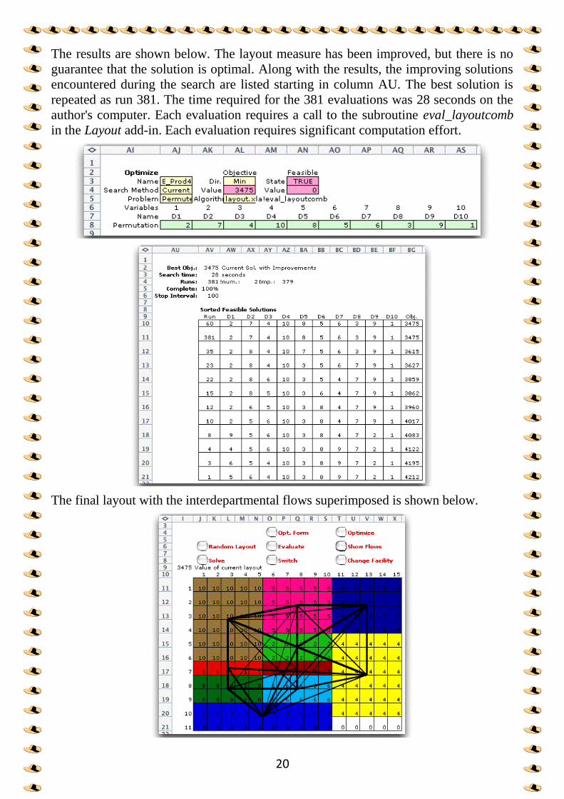
The results are shown below. The layout measure has been improved, but there is no

guarantee that the solution is optimal. Along with the results, the improving solutions

encountered during the search are listed starting in column AU. The best solution is

repeated as run 381. The time required for the 381 evaluations was 28 seconds on the

author's computer. Each evaluation requires a call to the subroutine eval_layoutcomb

in the Layout add-in. Each evaluation requires significant computation effort.

The final layout with the interdepartmental flows superimposed is shown below.

21

We see on the worksheet starting in column A, various quantities used in the

evaluation. When the combinatorial search procedures are in control, the sequence

defining the layout in column G is controlled by the the combinatorial algorithms. For

example, cell G11 holds the formula

=$AJ$8

The value in cell AJ8 is the first element of the permutation. The other cells in column

G are similarly linked to the combinatorial variables.

The combinatorial procedures of the Optimize add-in are much more powerful than

the random search and 2-way switches available in the Layout add-in. There are

limitations to the Optimize search however. Only the Sequential layout is defined by a

permutation, so the option is not available for the Traditional layout.

The combinatorial form (cells AN3 and AN4) allows feasibility conditions on

permutations. These are not used for the example, but the feasibility conditions might

be useful for other layout applications.

Assignment Costs and Restrictions

Clicking the Optimize Form button brings a dialog that controls whether the model

includes assignment costs and restrictions. We consider the same example as above,

but decide to include assignment costs. The Random data button indicates whether the

program is to provide random data for the costs. The Cost Density indicates the

proportion of cells that are to contain numeric cost data. The alternative is for a cell to

contain the string ***. This indicates that an assignment is not allowed.

22

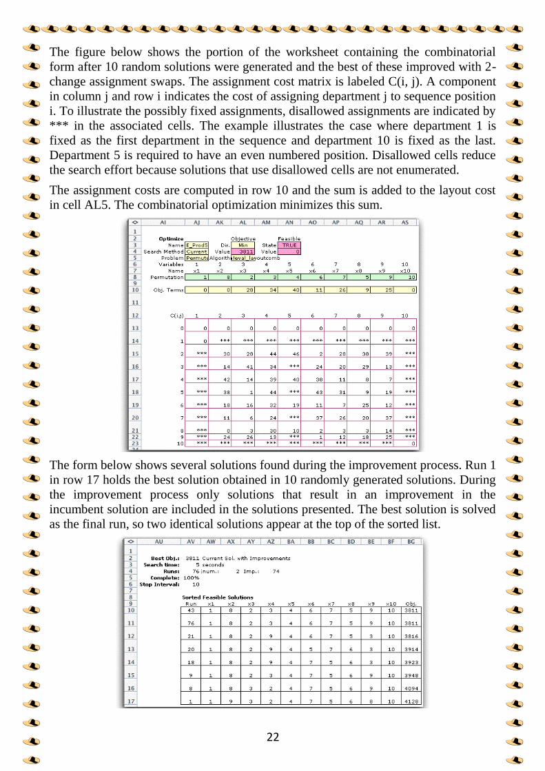
The figure below shows the portion of the worksheet containing the combinatorial

form after 10 random solutions were generated and the best of these improved with 2-

change assignment swaps. The assignment cost matrix is labeled C(i, j). A component

in column j and row i indicates the cost of assigning department j to sequence position

i. To illustrate the possibly fixed assignments, disallowed assignments are indicated by

*** in the associated cells. The example illustrates the case where department 1 is

fixed as the first department in the sequence and department 10 is fixed as the last.

Department 5 is required to have an even numbered position. Disallowed cells reduce

the search effort because solutions that use disallowed cells are not enumerated.

The assignment costs are computed in row 10 and the sum is added to the layout cost

in cell AL5. The combinatorial optimization minimizes this sum.

The form below shows several solutions found during the improvement process. Run 1

in row 17 holds the best solution obtained in 10 randomly generated solutions. During

the improvement process only solutions that result in an improvement in the

incumbent solution are included in the solutions presented. The best solution is solved

as the final run, so two identical solutions appear at the top of the sorted list.

23

The final layout is shown below.

It must be emphasized that the search processes provided by the Optimize add-in do

not guarantee optimality. They do provide a method to find good solutions to hard

problems. Using the random generation plus improvement options and few hours of

computation time, one can probably find good answers to problems of moderate size.

The effort to evaluate an individual layout grows approximately as the square of the

number of departments and linearly with the number of cells in the layout. The effort

of generating random solutions is approximately linear with the number of solutions

generated. The effort of one pass through the 2-change improvement process is

approximately quadratic with the number of departments. The number of passes

through the process is hard to estimate, but one would also expect that to grow with

the number of departments. The number of solutions evaluated for exhaustive

enumeration grows exponentially with the number of departments.

With these rough estimates, one could try exhaustive enumeration with up to 10

departments. From 10 -30 departments the various heuristics probably would yield

results in reasonable time. With more than 30 departments, quadratic growth begins to

become painful. With more than 30 departments, the cost of a commercial solver or

programming a stand alone application in an efficient programming language is

probably justified. The Excel worksheet can probably hold a problem with 100

departments, but computation would be painfully slow.