Facility Location under Demand Uncertainty:Response to a Large-scale Bioterror Attack

Abstract

In the event of a catastrophic bio-terror attack, major urban centers need to effi-

ciently distribute large amounts of medicine to the population. In this paper, we con-

sider a facility location problem to determine the points in a large city where medicine

should be handed out to the population. We consider locating capacitated facilities in

order to maximize coverage, taking into account a distance-dependent coverage func-

tion and demand uncertainty. We formulate a special case of the maximal covering

location problem (MCLP) with a loss function, to account for the distance-sensitive

demand, and chance-constraints to address the demand uncertainty. This model de-

cides the locations to open, and the supplies and demand assigned to each location.

We solve this problem with a locate-allocate heuristic. We illustrate the use of the

model by solving a case study of locating facilities to address a large-scale emergency

of a hypothetical anthrax attack in Los Angeles County.

Keywords: Capacitated facility location, distance-dependent coverage, demand un-

certainty, emergency response, locate-allocate heuristic

1 Introduction

Large-scale emergency events such as a bio-terrorist attack, or a natural calamity such as

an earthquake, strike with little or no warning. Such situations can lead to a big surge in

the demand for medical supplies. Implementing an efficient disbursement of the, possibly

limited, medical supplies needed to satisfy this demand is critical in reducing morbidity

and mortality. The United States maintains stockpiles of medical supplies, the Strategic

National Stockpile (SNS), to meet the extraordinary needs that can arise in such large-scale

emergencies. When the government declares the need to use the SNS, the initial supplies,

1

in the form of medical push packages, would be delivered at the affected location within 24

hours. The local authority is then responsible for developing an efficient plan for distributing

the supplies to the population.

A disbursement plan considered by local authorities consists of setting up points of dispersion

(POD) where the population would go to receive medical supplies or medical attention. This

form of distributing supplies is particularly useful if it is necessary to further screen the

population or have a trained team administer the medicine. The key decisions in setting up

such a disbursement plan consist of the locations of the facilities (or PODs) to be opened

and the amounts of supplies to stock at each of these facilities. Covering models are a classic

solution approach for facility location problems in emergency-related scenarios [Gendreau et

al. (2006) and Jia et al. (2006)]. A demand point is treated as covered only if a facility, or

a set of facilities, is available to provide the required service to the demand point within a

required distance or time. An important additional consideration when planning a response

to a large-scale emergency is that there is a large degree of uncertainty associated with the

location of the emergency and the number of people affected.

In this work we propose a capacitated facility location model to decide which facilities to open

as PODs and how many supplies to make available at each POD in order to maximize the

coverage of an uncertain demand in the event of a bio-terror attack. We make the following

assumptions about this large-scale emergency: 1) The fraction of the population at demand

point i that can be serviced by facility j decreases as distance dij increases. 2) The PODs

are capacitated facilities. 3) There is a total amount of supply S available to be distributed

among the facilities. 4) The demand is optimally assigned to facilities so that the demand

covered is maximized. The facilities are capacitated since the speed at which people are

serviced in a POD and the physical dimensions of these locations impose a restriction on the

maximum rate of service. Total supply constraints can be significant in an emergency setting

for a number of reasons, such as: the delay in delivery of the SNS, difficulty in estimating

the emergency demand, and concurrent demands on the SNS at other sites.

The assumption that an optimal assignment of demand points to facilities can be imple-

mented is a critical assumption of this model. When distributing medical supplies from

PODs, each individual has the freedom to decide whether to go to the assigned POD or to

deviate from this recommendation to obtain a better service, suggesting that a congestion

model would be a more representative model. We opted to consider a simple optimal as-

signment model of demand to facilities, as opposed to representing the congestion effects

of having individuals select facilities, since due to the uncertainty present in planning a re-

sponse to an emergency, the significance of a more representative demand model is not clear.

2

Such an optimal assignment model however is realistic when facilities send a mobile unit to

serve the population and it also has been a common practice to plan resources at facilities in

mandatory evacuation orders during hurricanes where people are advised to go to particular

relief centers [Sherali et al. (1991)]. We therefore assume that in a large-scale emergency,

local authorities aim for an efficient distribution of medical supplies by advising the affected

population to visit a particular set of facilities, based on their residential location, medical

conditions and supplies available at the facilities.

The question we seek to answer in this work is whether a facility location model with these

characteristics can obtain an efficient distribution of scarce medical supplies. This possibility

stems from the idea that a critical mistake would be to place the scarce supplies at locations

where they are not consumed due to the uncertainty in demand. We can avoid this by placing

the supplies at locations where they are more likely to be consumed. If we take into account

that a fraction of the demand can be covered by facilities that are further away, then the idea

is to select facilities at locations that could receive demand from more demand points and

are thus more likely to experience a stable demand. We develop efficient solution methods

for this optimization problem that allows us to solve real sized problems representing a large

urban area. We present computational results on a possible bio-terror attack in Los Angeles

County and simulated random demands to evaluate the solutions found.

The rest of the paper is organized as follows. In Section 2, we provide a brief review of prior

work on covering problems and stochastic facility location. In Section 3, we present the

proposed capacitated facility location model with chance-constraints, and in Section 4 we

present our solution algorithm to solve this optimization problem. We present results from

simulation experiments which verify the performance of our model and solution algorithm

in Section 5. Finally, in Section 6, we present our conclusions and some future work.

2 Literature Review

Given that our objective is to design an effective response strategy to a large-scale emergency

to reduce casualties, a maximal covering location problem (MCLP) [Church and ReVelle

(1974)] is appropriate for our purpose. In the event of a large-scale emergency, a very

important decision would be to locate facilities in tune with the location and intensity (that

is, number of affected people) of the attack. One of the key assumptions of the MCLP is

that a demand point is assumed to be fully covered if located within a distance r from the

facility and not covered if it is farther than r away from the facility. However, while planning

3

for an emergency scenario, due to the gravity of the situation, the possible damage to the

transportation network and individual decisions, it would be next to impossible to precisely

predict whether a person would be able/willing to travel to the recommended facility to

receive medicines, making it unrealistic to enforce the binary coverage assumptions of the

MCLP. Instead, it is more realistic to assume that the further away the facility is, the smaller

the fraction of the demand it can cover. In the generalized MCLP (GMCLP) as defined by

Berman and Krass (2002), each demand point i has multiple sets of coverage levels, with

corresponding coverage radii. That is, if a facility is located within a distance ri from i,

then the coverage level is ai(ri). The coverage levels can be thought of as a decreasing

step function of the distance between a demand point and an open facility. This work was

extended by Berman et al. (2003) to the gradual covering decay model where they considered

general forms of the coverage decay function. Berman et al. (2009) considered the variable

radius covering problem, where the decision-maker needs to determine coverage radii for the

facilities, in addition to the numbers and locations of facilities, to cover a discrete number

of demand points with minimal cost. In our work, we adopt the idea of multiple coverage

levels proposed by Berman and Krass (2002).

Previous works have considered a number of models of how demand is assigned to facilities.

Spatial interactions models, also known as “gravity models”, have been used by researchers

to assign demand to facilities as a function of parameters that could lead to attraction be-

tween demand points and facilities. Spatial interaction models such as those proposed by

Hodgson and Jacobsen (2009) propose a model based on the distance minimization approach

to represent how people assign themselves to facilities. Berman and Krass (1998) focus on

competitive facility location assuming that people decide which facility to visit based on

the facility’s attractiveness and the travel distance. Aboolian et al. (2007) study a location

problem wherein facilities compete for customer demand based on the service utility that

they provide. In these prior papers demand is assigned to facilities under competition or

congestion and every customer chooses a facility with an objective to maximize its individ-

ual utility leading to a game. Although such selfish behavior could occur in a large-scale

emergency, in this work we assume that demand is assigned optimally in order to maximize

the demand covered.

There exists a fair amount of literature on facility location models dealing with response to

an emergency. One of the earliest models in this area was developed by Toregas et al. (1971)

where they developed the location problem as a set covering problem with equal costs in the

objective. The sets were composed of the potential facility points within a certain distance

or time from each demand point. They solved this problem using linear programming tech-

niques. Rawls and Turnquist (2010) presented a two-stage stochastic optimization model

4

to locate facilities and assign supply to them under an emergency scenario. They develop

a mixed-integer program to address uncertainty in the demands and in the capacity of the

transportation network. Berman and Gavious (2007) presented competitive location models

to locate facilities that contain resources required for response to a terrorist attack. They

consider the worst-case scenario where the terrorist has knowledge of the location of the

facilities and the State needs to take this into account. Jia et al. (2006) presented an unca-

pacitated version of the covering model to locate staging areas in the event of a large-scale

emergency. The location of the facilities and the allocation of the demand points to the open

facilities are primarily based on distance constraints. In our paper, we extend this model

to a capacitated facility location model. Given the uncertainty associated with a large-scale

emergency, it is important to accurately determine the quantity of supplies to be stocked at

each potential facility site so that the coverage provided is maximized. To address this issue,

we consider the available supply at each facility to be a variable. Yi and Ozdamar (2007)

propose a mixed integer multi-commodity network flow model for logistics planning in emer-

gency scenarios. They address the aspects of distributing supplies to temporary emergency

centers and the evacuation of wounded people to emergency units. The location problem

is implicitly handled by allocating optimal service rates to emergency centers according to

which wounded patients are discharged from the system. Gormez et al. (2010) study the

problem of locating disaster response facilities to serve as storage and distribution points.

Under an emergency, supplies will flow from these facilities to local dispensing sites where

they will be distributed to people. They decompose the problem into a two-stage approach

- in the first stage, they decide the locations of the local dispensing sites, and in the second

stage they treat the local dispensing sites as demand points and decide the locations of the

response facilities. The model is solved for a worst-case earthquake scenario in Istanbul. Bal-

cik and Beamon (2008) develop a deterministic model that decides the number and locations

of stocking points in a humanitarian relief network and the type and amount of supplies to

be pre-positioned in these locations under budgetary and capacity constraints. Chang et al.

(2007) present a decision-making tool that could be used by disaster prevention and rescue

agencies for planning flood emergency logistics preparation. Two stochastic programming

models are developed to determine the structure of rescue organization, the location of res-

cue resource storehouses, the allocation of rescue resources within capacity restrictions and

the distribution of rescue resources.

Facility location models aid decisions that are expensive and difficult to change. Hence,

facility location models should consider the uncertainty associated with the demand, supply

and distance parameters over a time horizon. In the past, researchers have utilized stochas-

tic and robust optimization approaches to model uncertainty in facility location problems.

Snyder (2006) gives an in-depth review of the work done using these two approaches. Mean-

5

outcome models minimize the expected travel cost or maximize the expected profit. The

mean-outcome models introduced by Cooper (1974), Sheppard (1974) and Mirchandani and

Oudjit (1980) minimized expected costs or distance. Balachandran and Jain (1976) pre-

sented a capacitated facility location model with an objective to minimize expected cost of

location, production and transportation. Berman and Odoni (1982) considered travel-times

to be scenario-based, with transitions between states or scenarios occurring according to

a discrete-time Markov process. The objective was to minimize travel times and facility

relocation costs. Weaver and Church (1983), Mirchandani et al. (1985), Louveaux (1986)

and Louveaux and Peeters (1992) presented stochastic versions of the P-median problem

to choose facilities and allocate demand points. Berman and Drezner (2008) presented a

P-median problem that handles uncertainty by minimizing the expected cost of serving all

demand nodes in the future. Mean-variance models address the variability in performance

and the decision-maker’s aversion towards risk. Such models include Jucker and Carlson

(1976) and Hodder and Dincer (1986). Yet another method to model uncertainty is chance-

constrained programming. In this procedure, the parameters that are unknown at the time

of planning are assumed to follow certain probability distributions. A chance-constraint

requires the probability of a certain constraint, involving the uncertain parameter(s), hold-

ing to be sufficiently high. Carbone (1974) formulated a P-median model to minimize the

distance traveled by a number of users to fixed public facilities. The uncertainty in the num-

ber of users at each demand node is handled using chance-constraints. The model seeks to

minimize a threshold and ensure that the total travel distance is within the threshold with

a probability α. Interested readers are referred to Snyder (2006) and Snyder and Daskin

(2004) for a review of papers dealing with robust facility location.

While there exists a large amount of literature in the area of capacitated facility location,

there have not been many papers on maximal covering models that use chance-constraints to

deal with demand uncertainty. In an application like the one presented in this paper, where

the number of people affected by a large-scale emergency and its location are unknown well

in advance, facility location modeling under uncertainty is vital. Our model assigns the

supply to be stored at each facility by considering it as a decision variable that depends

on an unknown demand. Previous papers that have supply as a variable [Louveaux (1986)

and Rawls and Turnquist (2010)] do not consider the relation between supply and a random

unknown demand. Since the supply at each facility depends on a demand unknown to us

a-priori, we model this as a capacitated facility location problem and use chance-constraints

to handle the demand uncertainty.

6

3 Facility Location Model for Large-Scale Emergencies

In this section, we present the capacitated covering model with chance-constraints to handle

demand uncertainty. As explained earlier, our objective is to maximize the percentage of

the affected population that successfully receives the medication. That is, our goal is to

maximize coverage or minimize unmet demand.

3.1 Coverage Bound Function

In the work presented in this paper, we adopt the idea of multiple coverage levels introduced

by Berman and Krass (2002). We assume that the fraction of demand at point i that is

assigned by planners to any facility j to get service decreases with dij, the distance between

i and j. We assume this decrease follows a step function. That is, given positive distances

0 = δ0 < δ1 < δ2 < · · · < δK we let fkDi be the total demand from point i that can assigned

to the group of facilities located from δk−1 to δk, where Di is the demand of point i and K

is the number of coverage levels. The quantities fk denote the fraction of the demand at

i that can be satisfied in the interval of distance (δk−1, δk] from i. These fractions satisfy

1 = f1 > f2 > · · · > fK > 0. Since∑K

k=1 fk ≥ 1 is always valid, we enforce the condition

that∑

j∈J tij ≤ Di in the deterministic and chance-constrained models presented in the

following sections, where tij is the amount of medical supplies allocated to demand point i

by facility j. Note that we can have δK large enough to represent the maximum distance

local authorities would be willing to consider while assigning the affected population to open

facilities.

We illustrate the coverage bound function in Figure 1. Here, demand points are denoted

by stars and facilities by triangles. There are three coverage levels, shown by the concentric

circles around demand points. Facilities that fall beyond the third concentric circle of a

demand point, say i, are assumed to be too far to satisfy any of the demand of i. Demand

point 1 (DP1), with a demand of D1, has zero facilities in the first coverage level, two in

the second coverage level and zero in the third level. Following our coverage bound function,

facilities F1 and F3 can cover at most f2D1 of the demand of DP1. Since these are the

only two facilities in the area of coverage of DP1, the upper bound on the coverage DP1 can

obtain is the lowest of three quantities: f2D1, D1 and the total supply stored at facilities 1

and 3. Since F1 and F3 might also serve other demand points, the actual coverage DP1

will obtain could be lower than this upper bound. The other demand point, DP2, has one

facility in the first coverage level, one in the second level, and two facilities in the third

7

level. Hence, an upper bound on the coverage of DP2 is the minimum of three quantities:

f1D2 + f2D2 + f3D2, the demand D2, and the supply stored at F1, F2, F4 and F5. When

the sum of the fractions f1, f2 and f3 exceeds 1, then the maximum possible coverage is

limited by D2. Again, the actual coverage of the demand at DP2 could be lower than this

upper bound because F1, F2, F4 and F5 might need to serve other demand points as well.

Figure 1: Demand loss function

Note that the upper bound on the coverage at a certain coverage level is a property of the

demand and is not related to the number of facilities opened at that level. For example,

the bound on the coverage of DP2 at the third coverage level is at most f3D2 regardless of

whether both F1 and F2 are available or only one of them is open.

The covering model we present allows distributing the demand of one point between multiple

facilities located possibly at different coverage levels in order to maximize the amount of

demand serviced. For example, even if the facilities located in the first coverage level [0, δ1]

have sufficient supply to satisfy all the demand, it might be convenient to distribute some of

this demand to facilities at the second, or later, coverage levels, since the resources placed at

each facility need to satisfy the demand from other points also. In other words, the proposed

model maximizes the population covered by deciding which facilities to open, the quantity

of supplies to stock at each open facility, and how each demand point is serviced.

3.2 Deterministic Model

In the model presented below, we determine which of a set of pre-specified facilities need

to be opened when a large-scale emergency occurs. We consider a set I of demand points

and a set J of facility locations. We also consider that each demand point has K levels of

8

coverage. The model considers the following parameters and decision variables.

ParametersS : total supply available during an emergency

N : total number of facilities that need to be opened

βj : capacity of facility j ∈ J

Di : demand for medical supplies from demand point i ∈ I

fk : a fraction, fkDi is the k-th level coverage bound on the demand of point i

δk : radius of the k-th coverage level from a demand point

dij : distance between demand point i and facility j

Decision Variablesxj : takes a value of 1 if facility j ∈ J is open and 0 otherwise

sj : supply to be assigned to facility j ∈ J

tij : amount of medical supplies allocated to demand point i by facility j

In the deterministic model the location and the intensity (size of the affected population)

is known ahead of time. That is, the demand at each demand point is known. Then, the

problem at hand is to identify the locations of open facilities and their respective supplies,

sj, out of the available amount S so as to maximize coverage. The deterministic coverage

model is given below:

DM : max∑

i∈I,j∈J

tij

s.t.∑j∈J

xj = N (1)∑i∈I

tij ≤ sj ∀j ∈ J (2)

sj ≤ βjxj ∀j ∈ J (3)∑j∈J

sj ≤ S (4)∑j|δk−1<dij≤δk

tij ≤ fkDi ∀i ∈ I, k ∈ 1, . . . , K (5)∑j∈J

tij ≤ Di ∀i ∈ I (6)∑j|dij>δK

tij = 0 ∀i ∈ I (7)

xi ∈ {0, 1}; sj, tij ≥ 0

The objective of the above integer programming model is to maximize the number of people

who receive medication. The first constraint ensures that exactly N facilities are opened.

9

The second constraint ensures that the supplies distributed for all demand points from j

cannot exceed the available supply at j. Constraints (3) and (4) make sure supplies are only

assigned to open facilities and that these supplies satisfy the facility capacities and total

supplies available. The coverage bound function is enforced by constraint (5), where the

amount of demand that can be assigned to all the facilities within (δk−1, δk] of demand point

i is bounded by fkDi. The sixth constraint ensures that the amount of supplies assigned to

demand point i from all facilities (at all coverage levels) are not more than the demand at i,

Di. This way even if the∑K

k=1 fk ≥ 1, supplies sent to i do not exceed its demand.

3.3 Chance-constrained Model

We now consider the case when the demand for medical supplies at each demand point is not

known a-priori. This means that constraints 5 and 6 of DM have some degree of uncertainty

around them. We assume that the possible demand values due to an emergency event follow

a random variable for which we know the probability distribution at each demand point.

One solution in this case is to ignore the uncertainty, replace the random variable Di with

its expected value E [Di] and use the deterministic model DM to get a solution. However,

ignoring the uncertainty can be risky in emergency situations.

The proposed chance-constrained model instead requires that the uncertain constraints be

satisfied with high probability. That is, if we let ξi represent the random demand at i, the

fifth and sixth constraints of DM has to be satisfied except for a small probability ϵ ∈ (0, 1).

10

The chance-constrained model CCM is formulated as follows:

CCM : max∑

i∈I,j∈J

tij

s.t.∑j∈J

xj = N (8)∑i∈I

tij ≤ sj ∀j ∈ J (9)

sj ≤ βjxj ∀j ∈ J (10)∑j∈J

sj ≤ S (11)

Pr

∑j|δk−1<dij≤δk

tij ≤ fkξi

≥ 1− ϵ ∀i ∈ I, k ∈ 1, . . . , K (12)

Pr

(∑j∈J

tij ≤ ξi

)≥ 1− ϵ ∀i ∈ I (13)∑

j|dij>δK

tij = 0 ∀i ∈ I (14)

xi ∈ {0, 1}; sj, tij ≥ 0

The right hand side of constraints (12) and (13) (fkξi and ξi) and of the corresponding

constraints on DM represent an upper bound on the amount of demand from i that could be

satisfied by different groups of facilities. The chance constraint aims to identify an assignment

of demand to facilities tij that could meet the demand at the facilities with high probability.

In other words, regardless of how the demand ξi changes, the assignment to facilities ensures

that there is supply to satisfy some of this demand. We note that if the demand ξi turns

out to be higher than expected then the assignment to the supply in facilities tij would

satisfy only part of this demand. However, since we are maximizing∑

i∈I,j∈J tij, the amount

of demand that is satisfied is as large as possible, given the facility capacity and supply

constraints and distribution of demand. In practice, once facilities are opened and supply

levels assigned, when the emergency occurs and actual demand levels observed, a linear

optimization problem can be solved to determine optimal demand assignments.

While maximizing coverage, the CCM model assigns supply sj to facilities in J such that

facilities further away from demand points with ξi > 0 are allotted lower to little supply

compared to facilities closer to those demand points. This ensures that wastage of supplies

is minimized. We evaluate the suitability of the proposed approach in the experimental

section, where we perform simulations with random demand to observe how much of the

actual demand our chance-constrained model is able to satisfy.

11

In our work, we assume that the demand generated from the demand points follows a log-

normal distribution with mean µ′ and standard deviation σ′. We make this assumption

because demand generated at a demand point cannot be negative and the log-normal distri-

bution has a positive support. The relationship between the parameters of the log-normal

and the normal distributions are given by µ′ = log µ − 12σ′2, σ′2 = log(µ

2+σ2

µ2 ). We define κ

to denote the Z value of the normal distribution corresponding to the confidence level ϵ. κ

is called the safety factor, where ϕ (κ) = 1 − ϵ. Using this relation, we linearize the chance

constraint (12) as follows:

∑j|δk−1<dij≤δk

tij ≤ fkeµ′i−κσ′

i ∀i ∈ I, k ∈ 1, . . . , K . (15)

Chance constraint (13) can be linearized similarly.

The objective function for the chance-constrained model remains unchanged from the deter-

ministic model. We note that these linearized versions of the chance constraints (12) and

(13) have the same structure as constraints (5) and (6) on DM, with the demand value Di

replaced by eµ′i−κσ′

i . While in DM we replace Di by its expected value, in CCM we replace

it with the value given by the chance-constrained expression.

4 A Locate-Allocate Heuristic

The locate-allocate heuristic was introduced by Cooper (1974) and, for instance, used in

Larson and Brandeau (1986) to solve facility location problems. Jia et al. (2007) show that

the locate-allocate heuristic outperforms a genetic algorithm procedure and is nearly as good

as a Lagrangean-relaxation heuristic for solving an uncapacitated facility location problem

of locating medical supplies for a large-scale emergency. In terms of computational time,

they showed that the locate-allocate heuristic is much faster than a genetic algorithm and

a Lagrangean-relaxation heuristic. The efficiency shown for the uncapacitated version of

the problem suggest the use of this type of heuristic to solve the chance-constrained model

described previously. To describe the locate-allocate heuristic, we use the deterministic

model DM. To solve this heuristic for CCM, we need to simply replace Di with the value

given by the chance-constrained expression.

The idea behind this heuristic is very simple. The first step is to choose an initial location

for the N facilities to be opened. This can be done by using a simple greedy approach. In

our case, we solve an integer program with an objective to maximize the amount of supplies

12

transported between facilities and demand points. At this stage, we do not consider the

demand loss function, but simply specify that a facility is allowed to transport supplies to

demand points that lie within a radius δK from it. This mixed integer program IP1 is as

follows:IP1 : max

∑i∈I,j∈J

tij

s.t.∑j∈J

xj = N (16)∑i|dij≤δK

tij ≤1

N

∑i∈I

Di xj ∀j ∈ J (17)

xj ∈ {0, 1}; tij ≥ 0

The initial facilities opened, using IP1 above, consider the demand balanced over all open

facilities with the help of the second constraint. The second step of the heuristic is to allocate

demand points to the facilities that were opened, with an objective to maximize coverage.

In our case, we solve the following linear program LPA that does this allocation of demand

points to open facilities. We define a set J ′ to denote the set of facilities that have been

opened and ξiϵ as the demand realized at the confidence level of ϵ.

LPA : max∑

i∈I,j∈J ′

tij

s.t.∑i∈I

tij ≤ sj ∀j ∈ J ′ (18)

sj ≤ βj ∀j ∈ J ′ (19)∑j∈J ′

sj ≤ S (20)∑j∈J ′|δk−1<dij≤δk

tij ≤ fkξiϵ ∀i ∈ I, k ∈ 1, . . . , K (21)∑

j∈J ′|dij>δK

tij = 0 ∀i ∈ I (22)∑j∈J

tij ≤ ξiϵ ∀i ∈ I (23)

sj, tij ≥ 0

The third step of the locate-allocate heuristic is to create clusters of demand points served

by each open facility. Then, for each cluster, we try to relocate the open facility from its

current site to another one such that the total travel distance between the facility and the

demand points in the cluster is minimized. In our approach, we define clusters C1,. . . ,CN to

13

denote the N clusters formed by the N open facilities. The relocate integer program is:

IPR : min∑Cy

ΘCy ,j

∑i|i∈Cy

dij

s.t.

∑j∈J

xj = N (24)∑j

ΘCy ,j = 1 ∀y ∈ 1, . . . , N (25)∑Cy

ΘCy ,j = xj ∀j ∈ J (26)

xj ∈ {0, 1} ∀j ∈ J

Here, ΘCy,j is set to 1 if facility j is assigned to cluster Cy and 0 otherwise. The first constraint

ensures that every cluster is assigned exactly one facility, and the second constraint enforces

the condition that an open facility is assigned to only one cluster, and a closed facility is

assigned to none. On solving the above integer program, if a facility different from the one

used in the allocate step of the heuristic is found to minimize the total travel distance for any

particular cluster, then the new facility is assigned the same supply as the previous facility.

The allocate and relocate steps of the locate-allocate heuristic are repeated until no further

relocation occurs. At this stage, the heuristic is terminated. The favorable performance

of the location-allocation heuristic in solving facility location models has been presented

by Cooper (1964), Larson and Brandeau (1986), Densham and Ruston (1991) and Taillard

(2003) among others. In our implementation of this heuristic, we use integer programs to

solve the relocate and allocate procedures. This reduces the number of iterations required

to find the best set of locations and allocations. The heuristic stops when there is no further

reduction in the objective function value of the allocate step. While the convergence of the

heuristic cannot be proven for a general case, it did converge for all the instances in our

experiments. Its convergence for specific cases has also been discussed in the aforementioned

papers. In the following section, we test the performance of our heuristic and compare it

with a simulated annealing heuristic presented by Berman and Drezner (2006) which also

considers a distance-dependent demand.

5 Experimental Analysis

In this section, we present experiments to show how the deterministic and the chance-

constrained models and the locate-allocate heuristic can be used to locate staging areas for

14

mass distribution of the medical supplies with an objective to maximize coverage in the

event of an anthrax attack on Los Angeles County. Anthrax is a deadly disease that requires

vaccines and antibiotics to treat the affected persons and immunize the high-risk population.

During an anthrax emergency, the strategic national stockpiles (SNS) are mobilized for local

emergency medical services. We use the centroid of each census tract, representing the

aggregated population in that tract as the demand points. Using this procedure, we have

1939 demand points in Los Angeles County. Under a large-scale emergency scenario, the

demand arising from each demand point could be anywhere between 0 and the aggregate

population represented by it. The mean demand for the 1939 demand points were provided

to us. We were also provided with approximately 200 eligible facility sites. To protect

the confidentiality of the exact site locations, we use exactly 200 of these sites with a slight

perturbation in their geographical coordinates. Figure 2 shows the distribution of the demand

points in the County.

Figure 2: Locations of demand points within Los Angeles County

For the loss function, we consider three coverage levels of radii 4 mi, 8 mi and 12 mi re-

spectively, for every open facility. Corresponding to these coverage levels, we assume f1 =

100%, f2 = 65% and f3 = 30%. Additionally, as presented by Bravata et al. (2006), we

assume the supply of vaccines in each facility (βj) to be at least equal to 140,000 units per

week, with a response time period of 4 weeks. This means that the facilities have a supply

of 560,000 units. In the experiments below we take the total supply S to be some fraction

of the expected total demand. That is, we take S = γ∑

i∈I E[Di] for some service level

γ ∈ (0, 1]. We do this because the difficult situation is when there is a lack of supplies.

We coded the simulated annealing heuristic presented by Berman and Drezner (2006) in

C++ and ran it using Microsoft Visual Studio 5.0 on a Pentium IV computer with 512MB

15

RAM. We maintained the same settings as above, and compared its performance with our

locate-allocate heuristic. The simulated annealing heuristic uses an approach similar to that

of Vogel’s approximation method (Reinfeld and Vogel, 1958) to allocate demand points to

facilities. Since their heuristic does not consider supply as a variable, we assumed the capacity

of every open facility to be equal to the min(γ∑

i∈I E[Di]

N, βj). The demand experienced by a

facility is discounted as per the loss function. Facilities are sorted based on their opportunity

cost for which we used distance as a measure. Demand points are allocated to facilities as

long as the total demand assigned to a facility does not exceed its capacity.

The locate-allocate heuristic was coded in C++ using ILOG Concert Technology. For all the

experiments provided below, CPLEX and the locate-allocate heuristic were performed on a

Dell Precision 670 computer with a 3.2 GHz Intel Xeon Processor and 2 GB RAM running

CPLEX 9.0. The heuristics executed rather quickly in about 10-15 minutes. To contrast,

we compared the results obtained against solving the whole facility location problem with

CPLEX for 2.0 CPU hours keeping the best solutions found so far. The convergence of the

CPLEX solution slowed down considerably after 2.0 hours.

5.1 Deterministic Model

In this case, we use the mean demand for the 1939 demand points as the actual demand for

the respective demand points. We present below the coverage that could be obtained from

the deterministic model using the locate-allocate heuristic. We test the sensitivity of the

algorithm for varying number of facilities to be opened N and varying service levels γ.

γ 100% 90% 80% 70% 50% 30% 20%N=50 94.19 89.99 80 70 50 30 20N=40 89.66 88.32 80 70 50 30 20N=30 84.96 83.68 77.01 70 50 30 20N=20 74.56 72.26 72.09 70 50 30 20

Table 1: Coverage from the deterministic model using locate-allocate heuristic

We compare the above results with that obtained by using the simulated annealing procedure,

presented by Berman and Drezner (2006), to solve the deterministic facility location problem.

The results from the simulated annealing procedure are presented below.

In the figure below we plot the performance of the locate-allocate (L-A) heuristic and the

simulated annealing (SA) procedure for N = 40, and compare them to the best lower bound

16

γ 100% 90% 80% 70% 50% 30% 20%N=50 90.86 84.71 79.96 70 50 30 20N=40 82.45 80.24 77.58 69.97 50 30 20N=30 79.67 76.44 74.30 69.89 50 30 20N=20 71.34 69.91 68.83 68.67 50 30 20

Table 2: Coverage from the deterministic model using the simulated annealing heuristic

(LB) and upper bound (UB) of the integer program DM obtained using CPLEX after 2.0

CPU hours, also for N = 40. Figure 3 shows that for the settings of our problem, the locate-

20 30 40 50 60 70 80 90 10020

30

40

50

60

70

80

90

100

Service Level (%)

Cov

erag

e (%

)

Coverage at N = 40

L−ASALBUB

Figure 3: Comparison of locate-allocate and simulated annealing for N = 30

allocate heuristic outperforms the simulated annealing procedure in locating facilities to

maximize coverage. In addition, while the coverage achieved by the locate-allocate heuristic

is mostly greater than the CPLEX lower bound, the coverage achieved by simulated annealing

is usually slightly below this lower bound for γ values of 100%, 90%, and 80%. This trend

in both the heuristics holds true for the all the values of N tested, as shown in Tables 1 and

2 above.

To further evaluate the performance of our algorithm in comparison to that of simulated

annealing, we design an experiment that consists of 500 demand points and 50 potential

facility sites. The demand points and facility sites were chosen randomly from the entire set

for Los Angeles that was presented earlier. As before, βj = 140,000 units per week and γ =

[0,1] and the response time is 4 weeks. We solve the deterministic problem DM using L-A

and SA for different coverage levels radii (r) and coverage fractions (f) : r1 = 4 mi, 8 mi,

17

12 mi; r2 = 3 mi, 6 mi, 12 mi; f 1 = 100%, 65%, 30%; f 2 = 100%, 75%, 50%. The results of

these experiments are presented in Tables 3 - 8 below.

γ 100% 90% 80% 70%N=20 95.62 90 80 70N=10 86.49 83.25 76.80 69.79N=5 75.44 73.37 69.64 64.76

Table 3: Coverage from DM using L-A heuristic, under r1 and f 1

γ 100% 90% 80% 70%N=20 91.41 87.31 80 70N=10 79.11 72.73 65.35 53.33N=5 70.47 61.93 53.80 43.71

Table 4: Coverage from DM using SA heuristic, under r1 and f 1

γ 100% 90% 80% 70%N=20 98.74 90 80 70N=10 89.56 85.67 78.25 70N=5 75.81 73.37 69.64 64.76

Table 5: Coverage from DM using L-A heuristic, under r1 and f 2

On comparing results in Tables 3 and 4, we conclude that L-A outperforms SA under these

settings. We also note that for both heuristics the coverage drops when the number of

open facilities is 5. This could be due to the fact that 5 facilities may not be sufficient to

provide reasonable coverage to the spatially distributed demand points. There is a slight

improvement in coverage when the coverage fractions increase (Table 5). This could mean

that the total supply, S, stored at the open facilities in the experiments in Table 3 was

less than 4Nβj, where N is the number of open facilities and the response time is 4 weeks.

On increasing the coverage fractions, some of the remaining supply can now be allotted to

demand points in all three coverage levels, thereby increasing overall coverage. However, the

improvement in coverage is negligible with 5 open facilities probably because S was very close

to 4Nβj and very few of the 500 demand points are within 12 miles from the open facilities.

If S ≈ 4Nβj under f 1, then little supply is left over for allocation to demand points upon

increasing coverage fractions. The coverage remains unchanged because the optimal solution

obtained with the original coverage fractions would still remain optimal.

Similar to the previous set of experiments, we notice from Tables 6 and 7 that L-A performs

better than SA. Once again coverage slightly improves when coverage fractions are increased.

18

γ 100% 90% 80% 70%N=20 89.22 84.36 77.53 70N=10 76.48 74.57 70.70 66.15N=5 69.61 69.01 67.14 63.79

Table 6: Coverage from DM using L-A heuristic, under r2 and f 1

γ 100% 90% 80% 70%N=20 82.57 76.41 73.13 68.93N=10 68.62 61.43 55.89 50.44N=5 63.13 57.10 49.60 40.57

Table 7: Coverage from DM using SA heuristic, under r2 and f 1

However, the gain in coverage obtained in Table 8 is lower than the gain obtained in Table

5. This could mean that a significant number of demand points were located between 3 and

4 miles and between 6 and 8 miles from the open facilities. Demand points located between

3 and 4 miles could receive up to 100% coverage in the first set of experiments, but only up

to 75% in the second set. Demand points located between 6 and 8 miles could receive up to

75% coverage in the first set of experiments, but up to 50% in the second set. Hence, the

gain is lower in Table 8.

5.2 Chance-constrained Model

Having verified the quality of the locate-allocate heuristic for solving the deterministic model,

we now investigate the performance of the chance-constrained model and the heuristic under

demand uncertainty. For all the results presented in this section, we assume that N = 20

and γ = 0.8. We use a log-normal distribution with the same mean values as was used in

the deterministic case for generating random demand for the simulations presented in this

section. The standard deviations are taken to be a certain percentage (10%, 20% etc.) of the

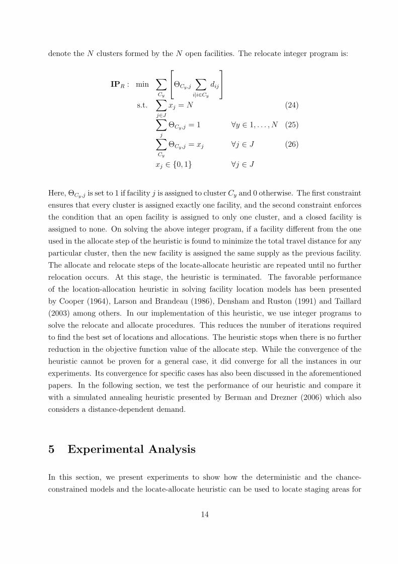
respective mean demand values. In Table 9 below, we present the results from an experiment

γ 100% 90% 80% 70%N=20 91.52 85.25 77.79 70N=10 77.83 75.33 70.78 66.21N=5 69.61 69.01 67.14 63.79

Table 8: Coverage from DM using L-A heuristic, under r2 and f 2

19

to study how the κ values impact the coverage provided by the chance-constrained model.

κ ϵ σ=10% σ=20% σ=40%1.96 0.025 62.52 52.57 41.621.64 0.050 63.47 53.16 42.111.44 0.075 64.08 53.38 42.651.28 0.100 64.66 54.09 44.831.15 0.125 64.94 55.13 45.541.04 0.150 65.18 56.69 46.730.93 0.175 65.27 57.21 48.440.84 0.200 65.78 59.32 49.23

Table 9: Coverage from the chance-constrained model

For low values of ϵ (corresponding to high values of κ and low uncertainty), the constraint

that∑

j tij should never exceed fkξiϵ can be satisfied easily. Hence,

∑j tij ≤ fkξ

iϵ is a tight

constraint. This explains the low coverage values in Table 9 above. As ϵ increases (that is,

uncertainty increases), ξiϵ would need to be set to a higher value so that∑

j tij never exceeds

fkξiϵ. As a result, coverage values increase.

Next, we perform two sets of simulation experiments to evaluate the quality of the locations

of the open facilities and the supply stored at each open facility in terms of unmet demand

through simulations. For both the simulation experiments, we fix the facility locations and

supplies, that is, the xj and sj solution values for all the locations, for each combination of

κ and σ as per Table 9. Next, we generate random demands for the 1939 demand points

based on their respective mean values for each value of σ. We compute the following for

each sample of demand: (1) the coverage of the CCM from the performance obtained by the

facility sites and supply solutions under this random demand for a given κ-σ combination

is recorded as the coverage obtained by using the CCM for allocating demand points to

facilities, (2) coverage obtained if demand were known in advance (i.e., deterministic) in

which case the DM model is used for locating facilities and allocating demand points and

supplies to facilities. Then, the ratios (1)(2)

are computed. Each recording in Table 10 below

is the average of 20 such ratios.

The ratios compare the performance of facility locations and their respective supplies out-

putted by the CCM model under a random demand to the performance of the locations

and their supplies outputted by the DM model optimal for that demand alone. In Table 10,

the denominator values remain constant for each column. Similar to Table 9, the numerator

values increase with a decrease in the κ value and decrease with an increase in uncertainty,

represented by the standard deviation. Table 10 shows that in the worst case, the locations

20

chosen by the locate-allocate heuristic cover approximately 69% of the demand that could

be covered had we known this random demand well in advance. For the best-case scenario,

this value increases to approximately 86%.

κ ϵ σ=10% σ=20% σ=40%1.96 0.025 0.8253 0.7386 0.68681.64 0.050 0.8352 0.7558 0.70781.44 0.075 0.8391 0.7734 0.73121.28 0.100 0.8502 0.7815 0.74571.15 0.125 0.8539 0.8040 0.74921.04 0.150 0.8606 0.8121 0.75980.93 0.175 0.8626 0.8200 0.77040.84 0.200 0.8646 0.8317 0.7844

Table 10: Ratio of the coverage from the CCM under a random demand to the best possiblecoverage had we known this demand in advance

For the second simulation experiment, we compute the following: (1) the numerator is

computed just as how they were computed in Table 10 above, (2) we consider the sites, the

xj and the sj values, used by the deterministic model, presented in Table 1 with N = 20

and γ = 0.8 and allocate demand points to these open facilities under the same demands as

were considered for the numerator (1). Then, the ratios (1)(2)

are computed. Each recording

in Table 11 is averaged over 20 such ratios.

κ ϵ σ=10% σ=20% σ=40%1.96 0.025 0.9799 0.9820 1.01521.64 0.050 0.9917 1.0048 1.07271.44 0.075 0.9962 1.0282 1.10821.28 0.100 1.0094 1.0390 1.13011.15 0.125 1.0138 1.0689 1.13531.04 0.150 1.0218 1.0797 1.15140.93 0.175 1.0242 1.0902 1.16750.84 0.200 1.0265 1.1058 1.1887

Table 11: Ratio of the performance of the CCM to theDM in response to a random demand

Table 11 shows the merit of using the chance-constrained model to locate facilities, determine

their supplies and allocate demand points to the open facilities. It also shows the relative

gain in the coverage, achieved by using the chance-constrained model over the deterministic

model, increases with a decrease in the safety factor and an increase in the standard deviation.

The first is due to an increase in the numerator values as κ decreases, and the second is due

21

to a decrease in the denominator values as demand uncertainty increases. Under the best-

case scenario, we see nearly a 20% gain in coverage by resorting to the locations given by

the chance-constrained model.

6 Conclusions

In this study, we consider the problem of locating points of disbursement (POD) for medicines

in response to a bio-terror attack. To address the tremendous magnitude and low frequency

of large-scale emergencies we obtain a solution that maximizes the number of people serviced

under such uncertain and limited resources/time conditions.

The main contribution of our work is in designing a response strategy to distribute supplies

in a large-scale emergency that considers distance-sensitive coverage, in addition to demand

uncertainty. In the problem we consider here, first, the facilities are capacitated by the

service rate of a POD. Second, the demand satisfied depends on the distance to the facility.

This is because while planning response to a large-scale emergency scenario, it is reasonable

to assume that the number of people expected to be assigned to a particular POD decreases

as their distance to that POD increases. Thirdly, given the unpredictability as to when and

where such an emergency scenario could occur and how many people would be affected, there

is a significant uncertainty in demand values. The aim is to identify locations and a way of

distributing supplies that will be effective in meeting the uncertain demand. In an emergency

situation an overriding objective is to service as much of the demand as possible. In such a

situation, an effective placement of supplies so that they service demand is more important

than an accurate model of how demand is distributed among facilities. Finally in this work

we aim to include the aggregate effect of uncertainty in the demand at different facilities and

leave for future work the inclusion of more detailed demand distribution models, such as a

consumer-choice demand model.

7 Acknowledgements

This research was partly supported by the United States Department of Homeland Security

through the Center for Risk and Economic Analysis of Terrorism Events (CREATE) at

USC. The findings, conclusions and recommendations presented in this paper are those of

the authors, and do not necessarily reflect the views of the Department of Homeland Security.

22

The authors would like to thank Hongzhong Jia, Yen-Ming Lee, Wei Ye and Zhihong Shen

for their help and valuable inputs through the course of this research work. We also thank

the anonymous referees for their valuable suggestions to help us improve the paper.

23

References

[1] Aboolian, R., Berman, O., and Krass, D. Competitive facility location and

design problem. Eur J Opl Res 182 (2007), 40–62.

[2] Balachandran, V., and Jain, S. Optimal facility location under random demand

with a general cost structure. Nav Res Logist Q 23 (1976), 421–436.

[3] Balcik, B., and Beamon, B. M. Facility location in humanitarian relief. Int J

Logist: Res Appl 11 (2008), 101–121.

[4] Berman, O., and Drezner, Z. Location of congested capacitated facilities with

distance-sensitive demand. IIE Trans 38 (2006), 213–231.

[5] Berman, O., and Drezner, Z. The P-median problem under uncertainty. Eur J

Opl Res 189 (2008), 19–30.

[6] Berman, O., Drezner, Z., Krass, D., and Wesolowsky, G. O. The variable

radius covering problem. Eur J Opl Res 196 (2009), 516–525.

[7] Berman, O., and Gavious, A. Location of terror response facilities. Eur J Opl Res

177 (2007), 1113–1133.

[8] Berman, O., and Krass, D. Flow intercepting spatial interaction model: a new

approach to optimal location of competitive facilities. Location Science 6 (1998), 41–

65.

[9] Berman, O., and Krass, D. Generalized maximum cover location problem. Comput

Oper Res 29 (2002), 563–581.

[10] Berman, O., Krass, D., and Drezner, Z. The gradual covering decay location

problem on a network. Eur J Opl Res 151 (2003), 474–480.

[11] Berman, O., and Odoni, A. R. Locating mobile servers on a network with Marko-

vian properties. Networks 12 (1982), 73–86.

[12] Bravata, D. M., Zaric, G. S., Holty, J.-E. C., Brandeau, M. L., Wilhelm,

E. R., McDonald, K. M., and Owens, D. K. Reducing mortality from anthrax

bioterrorism: Costs and benefits of alternative strategies for stockpiling and dispensing

medical and pharmaceutical supplies. Biosecurity and Bioterrorism, Biodefense Strat-

egy, Practice and Science 4 (2006), 244–262.

24

[13] Chang, M. S., Tseng, Y. L., and Chen, J. W. A scenario planning approach

for the flood emergency logistics preparation problem under uncertainty. Transport Res

Part E 43 (2007), 737–754.

[14] Church, R., and ReVelle, C. The maximum covering location problem. Papers of

the Regional Science Association 32 (1974), 101–118.

[15] Cooper, L. Heuristic methods for location-allocation problems. SIAM Review 6

(1964), 37–53.

[16] Cooper, L. A random locational equilibrium problem. J Regional Sci 14(1) (1974),

47–54.

[17] Densham, P., and Rushton, G. Designing and implementing strategies for solving

large location-allocation problems. Tech. rep., National Center for Geographic Informa-

tion and Analysis, 1991.

[18] Frank, H. Optimum locations on a graph with probabilistic demands. Oper Res 14(3)

(1966), 409–421.

[19] Gendreau, M., Laporte, G., and Semet, F. The maximal expected coverage

relocation problem for emergency vehicles. J Opl Res Soc 57 (2006), 22–28.

[20] Gormez, N., Koksalan, M., and Salman, F. S. Locating disaster response facil-

ities in istanbul. J Opl Res Soc (2010), 1–14.

[21] Hodder, J. E., and Dincer, M. C. A multifactor model for international plant

location and financing under uncertainty. Comput Oper Res 13(5) (1986), 601–609.

[22] Hodgson, M. J., and Jacobsen, S. K. A hierarchical location-allocation model

with travel based on expected referral distances. Ann Oper Res 176 (2009), 271–286.

[23] Jia, H., Ordonez, F., and Dessouky, M. M. A modeling framework for facility

location of medical services for large-scale emergencies. IIE Trans 39 (2006), 41–55.

[24] Jia, H., Ordonez, F., and Dessouky, M. M. Solution approached for facility

location of medical supplies for large-scale emergencies. Comput Indus En 52 (2007),

257–276.

[25] Jucker, J. V., and Carlson, R. C. Public facilities location under a stochastic

demand. Oper Res 24(6) (1976), 1045–1055.

[26] Jucker, J. V., and Carlson, R. C. The simple plant location problem under

uncertainty. Oper Res 24(6) (1976), 1045–1055.

25

[27] Larson, R. C., and Brandeau, M. Extending and applying the hypercube queuing

model to deploy ambulances in boston. Delivery of Urban Services (1986), In: Swersey,

A. and Ignall, E. (eds.).

[28] Louveaux, F. V. Discrete stochastic location models. Ann Oper Res 6 (1986), 23–34.

[29] Louveaux, F. V., and Peeters, D. A dual-based procedure for stochastic facility

location. Oper Res 40(3) (1992), 564–573.

[30] Mirchandani, P. B., and Oudjit, A. Localizing 2-medians on probabilistic and

deterministic tree networks. Networks 10(4) (1980), 329–350.

[31] Mirchandani, P. B., Oudjit, A., and Wong, R. T. Multi-dimensional extensions

and a nested dual approach for the m-median problem. Eur J Opl Res 21(1) (1985),

121–137.

[32] Rawls, C. G., and Turnquist, M. A. Pre-positioning of emergency supplies for

disaster response. Transport Res Part B 44 (2010), 521–534.

[33] Reinfeld, N. V., and Vogel, W. R. Mathematical Programming. Prentice-Hall,

Englewood Cliffs, New Jersey, 1958.

[34] Sheppard, E. S. A conceptual framework for dynamic location-allocation analysis.

Environment and Planning A 6 (1974), 547–564.

[35] Sherali, H. D., and Carter, T. B. A location-allocation model and algorithm for

evacuation planning under hurricane/flood conditions. Transport Res Part B 25 (1991),

439–452.

[36] Snyder, L. Facility location under uncertainty: A review. IIE Trans 38(7) (2006),

537–554.

[37] Snyder, L., and Daskin, M. S. Stochastic p-robust location problems. IIE Trans

38(11) (2006), 971–985.

[38] Taillard, E. D. Heuristic methods for large centroid clustering problems. J Heuristics

9 (2003), 51–73.

[39] Toregas, C., Swain, R., ReVelle, C., and Bergman, L. The location of emer-

gency service facility. Oper Res 19 (1971), 1363–1373.

[40] Weaver, J. R., and Church, R. L. Stochastic p-robust location problems. Trans-

portation Science 17(2) (1983), 168–180.

26

[41] Yi, W., and Ozdamar, L. A dynamic logistics coordination model for evacuation

and support in disaster response activities. Eur J Opl Res 179 (2007), 1177–1193.

27