Embed Size (px)
Citation preview

05METALS ENVIRONMENTAL RISK ASSESSMENT GUIDANCE
MERAGBioavailability: water, soils and sediments
MAY 2016
Check you have the most recent fact sheet by visiting www.icmm.com
FACT SHEET

CONTENTS
01. Introduction 02
02. Concepts and overview
2.1 Terminology and Definitions 03
2.2 Tiered approaches for using bioavailability 06
2.3 Data availability for the bioavailability assessment/normalisation 10
03. Implementation of bioavailability: water
3.1 General concept 14
3.2 Use of “total dissolved” metal 15
3.3 Use of “dissolved metal species of concern (DMSC)” 21
3.4 Development and application of toxicity-related bioavailability models 27
3.5 Importance of dietary route of toxicity of metals 43
04. Implementation of bioavailability: sediment
4.1 General concept 45
4.2 Equilibrium partitioning approach 46
4.3 Physico-chemical speciation modeling 47
4.4 Use of toxicity-related bioavailability models 50
4.5 Tiered implementation in a risk assessment context. 51
4.6 Relative importance of dietary route for metals in sediments 61
05. Implementation of bioavailability: soil
5.1 Introduction 62
5.2 General concept 64
5.3 Mechanistic versus empirical terrestrial bioavailability models 64
5.4 Toxicity-related bioavailability models 69
5.5 Implementation of bioavailability corrections into the derivation of
soil threshold concentrations 81
References 94
MERAG Fact Sheet 5 – May 2016
2
1. INTRODUCTION
The degree to which metals are available and cause toxicity to aquatic, sediment-burying and
terrestrial organisms is determined by site-specific geochemical conditions controlling the
speciation/precipitation and/or complexation of metals. In the aquatic environment, these
processes are generally controlled by pH and DOC (dissolved organic carbon). Furthermore,
several cations (Ca, Mg, Na, K) are known to compete with metal ions for binding to the site of
toxic action and hence have the potential to reduce metal toxicity. In sediments, sulfides,
organic carbon and iron/manganese (oxy)hydroxides play a mitigating role as they provide
important binding/absorption phases. For the soil compartment, it has been demonstrated that
clay minerals, organic carbon and soil pH are the main drivers controlling bioavailability of
metals. The wide variation of the physico-chemical characteristics encountered in the
environment is the main reason why no clear relationships have been observed between
measured total concentrations of metals and their potential to cause toxic effects. Therefore,
taking bioavailability into account will improve traditional environmental assessment approaches
as it helps to increase the realism of the assessment and can help regulators to better
understand the likelihood of the occurrence of adverse effects due to metal contamination.
The information presented in this document serves as guidance both for the national
governmental institutions, industrial users and evaluating experts faced with implementing
bioavailability for inorganic substances. This guidance provides the key scientific principles,
tiered approaches and a step-by-step explanation that can be used to implement bioavailability
for the water, sediment and soil compartments. As hazard data are a key component of setting
safe ecotoxicity thresholds for metals, the guidance focuses on how bioavailability corrections
can be applied for the purpose of using the normalised hazard data into a risk assessment
framework. Two areas that this guidance does not cover are 1) the influences of multi-metal
mixtures or multiple metals in media and 2) marine environments are not covered. Although Cu,
Zn, and Ni have data on these areas, data for most other metals are scarce.
The structure of this guidance is the following: in section 2, a brief overview is given of the
terminology and definitions used and the tiered approaches are introduced that can be used in
implementing bioavailability. In section 3 each environmental compartment (water, sediment
and soil) is outlined in detail with the specific steps needed to take bioavailability into account.
For the water compartment, different approaches are presented going from measuring
dissolved metal concentrations up to the use of more advanced tools such as the Biotic Ligand

MERAG Fact Sheet 5 – May 2016
3
Model (BLM). For sediments, binding to different sediment phases (sulfides, organic carbon and
Fe, Al Mn-oxy hydroxides) as key parameters controlling metal bioavailability are being
explored. For soil, next to the aspect of bioavailability, time-related features such as lab-to-field
extrapolations are covered. Finally, specific examples on how to implement bioavailability are
presented in every section.
2. Concepts and overview
2.1 Terminology and Definitions
The “bioavailability” concept encompasses several operationally defined and interacting terms
(Figure 1) and the interpretation may differ depending on the context used (human health vs
environmental research, type of regulation, etc). Availability starts with physico-chemical
considerations (chemical availability) but should be subsequently linked to different ecological
receptors taking different uptake routes into account (ECHA 2014).
Figure 1: Simplified conceptual outline for metals bioavailability (after M. McLaughlin personal
communication). (“Men+
” refers to the free metal ion.)
MERAG Fact Sheet 5 – May 2016
4
The following definitions apply (to metals) in this fact sheet:
Bioaccessible fraction: is the fraction of the environmental available metal that actually
interacts at the organism‟s contact surface and is potentially available for absorption or
adsorption by the organism.
Bioavailability: (or biological availability) means the extent to which a substance is taken
up by an organism, and distributed to an area within the organism. “It is dependent upon
physico-chemical properties of the substance, anatomy and physiology of the organism,
pharmacokinetics, and route of exposure.” (UN-GHS 2013). Hence, metal bioavailability
refers to the fraction of the bioaccessible metal pool that is available to elicit a potential
effect following internal distribution: metabolism, elimination and bioaccumulation. For the
purpose of this guidance, the term “metal bioavailability” is used more as a conceptual term
as initially proposed by Meyer (2002).
Biogeochemical region: Fairbrother and McLaughlin (2002) initially referred to this concept
as metallo-regions where on a regional scale separate sub-regions are being defined using
suitable methods to aggregate spatially explicit environmental variables. Another term
frequently used in this regard is “ecoregion”. At the moment the biological/ecological-part
has been a bit underrated as the current existing biogeochemical regions are based on
abiotic factors rather than quantified ecological metrics. If ecology can be considered,
instead of using „generic‟ species, it is preferable to use „endemic‟ test organisms
representative for the natural environment under investigation to characterise the sensitivity
of the ecosystem.
Biotic ligand: Metal toxicity is simulated as the accumulation of metal at a biologically
sensitive receptor, the “Biotic Ligand”, which represents the site of action for metal toxicity. It
is hypothesised to be placed on the gill surface.
Critical biotic ligand accumulation: is the critical concentration referred to as the “LAx",
or the (sub)lethal accumulation of metal on the biotic ligand associated with x% effect.
Critical bioavailable dissolved concentration: is the critical ligand concentration
recalculated to the specific physico-chemistry conditions occurring at a site and expressed
as dissolved concentration.
Environmental threshold value (ETV): is an environmental effects concentration below
which adverse effects on the environment are not expected to occur. Examples of ETVs are
Predicted No Effect Concentrations (PNEC), Environmental Quality Standards (EQS), Water
Quality Criteria (WQC), Water Quality Standards etc.
MERAG Fact Sheet 5 – May 2016
5
Environmental exposure concentration (EEC): is an exposure benchmark value, which is
compared with an ETV in a risk assessment framework or for compliance checking. The
EEC is typically calculated from all individual measured or modelled metal concentrations for
a predefined environment taking a high end value (eg the 90th percentile) of the
environmental concentration distribution at a site/region.
Environmentally available fraction: is the portion of total metal in soil, sediment, water
and air that is available for physical, chemical, and biological modifying influences (eg fate,
transport, bioaccumulation). It represents the total pool of metal at a given time in a system
that is potentially bioavailable (McGeer et al 2004; US EPA 2007).
Reasonable worst case conditions (RWC): are considered to be the environmental
conditions that maximize bioavailability.
Several metrics have been put forward to assess bioaccessibility and bioavailability. None of
them can really be singled out to capture all the different aspects in relation to bioavailability of
chemicals in general (ECHA 2014) and some have a broader and more relevant applicability
domain then others (eg free ion vs dissolved concentrations). For metals, the free metal ion and
its potential to complex/compete with other organic and inorganic ligands for the available
biological binding sites and its internal distribution within an organism is key to understanding
metal availability. It is acknowledged that the free ion is not necessarily the best predictor for all
metals because other metal species such as neutral species (eg AgCl, HgS) and anionic
species (eg SeO2-, AsO42-) may contribute to the observed toxicity (Campbell 1995). Taking into
account the different processes and metal forms that could occur in an ambient water and/or
test medium, the following operationally defined terms will also be used to make a distinction
between “Total metal”, “Total dissolved metal” and “Dissolved metal” species of concern:
Total metal concentration: comprises particulate (adsorbed/absorbed + precipitated) +
dissolved (inorganic complexes + organic complexes + free ionic forms);
Total dissolved metal concentration: refers to the fraction that passes through a filter of
0.45 µm and comprises inorganic complexes + organic complexes + free ionic forms;
Dissolved metal species of concern: refers most often to the free metal ion, but other
relevant metal speciation forms that could contribute to the observed toxic effect are also
covered.
Over the last decade, significant efforts have been conducted to embed bioavailability concepts
in predictive models such as the Biotic Ligand Model (BLM), SEM-AVS concept (SEM =

MERAG Fact Sheet 5 – May 2016
6
Simultaneously Extracted Metals; AVS = Acid Volatile Sulfides) and soil/sediment regression
models1. Bioavailability models have become recognised and discussed within the regulatory
community (US-EPA 2007; ECHA 2008; Ahlf et al 2009; Ruedel et al 2015). However, their
implementation in the past has been lagging behind due to the lack of regular fit/science
development and the availability of suitable and/or properly validated tools. Currently, the
applicability and data needs of the different Biotic Ligand Models have been validated in some
countries (UK, France) (David et al 2011) and more validated friendly-to-use models have been
developed (Bio-met 2011).
Validation of the bioavailability models should both consider internal validation (ie, how well
does a model predict based on the data on which the model was developed) and external
validation (ie, how well can the model be used to give sound predictions of future settings).
Similar OECD validation principles apply for the development and application of Quantitative
Structure-activity Relationship (QSAR) models (OECD 2014a). As models get proper validation,
it can be expected that these models may gain importance and be implemented more in the
regulatory scene. However, even if a model has been validated, it is clear that the applicability
domain of the current BLM models does not cover all relevant metal species. For example the
BLM model/free ion concepts are less suited to predict effects of metal particulates (eg physical
effects as clogging gills), transformation to organometallics (eg methylation), release of
hydrophobic organometallic and organic metal salts (OMS) (OECD 2014b), bioavailable low
molecular weight complexes (eg metals bound to natural dissolved organic matter), other
inorganic metal species such as AgCl, HgS (Campbell 1995), cationic inorganic complexes (eg
Cd(OH)+) etc.
2.2 Tiered approaches for using bioavailability
Depending on the knowledge level for the metal/metal compound under investigation,
bioavailability for the aquatic compartment (water and sediment) and soil can be introduced in a
tiered approach as depicted in Figure 2.
1 Regression models are empirical models that allow prediction of toxicity by using a regression equation derived from
bivariate experiments.

MERAG Fact Sheet 5 – May 2016
7
Figure 2: Refinement levels for the incorporation of bioavailability concept for the water, sediment and
soil compartment. Where SS = suspended solids; AVS = Acid Volatile Sulfides; OC = organic carbon;
Fe/Mn = iron/manganese hydro-oxides.)
A summary of the rationale for each refinement step for the different environmental
compartments is given below. The sections where the methodological steps are covered in
more detail are indicated between brackets.
Water compartment
Tier 1 (see section 3.2): For water, measuring dissolved metal concentrations is preferred
because total metal concentrations are a poor predictor of metal toxicity to aquatic organisms.
Although measuring dissolved concentrations is becoming more and more common, sometimes
only total concentrations are available. In that case, if information is available on the amount of
suspended solids (SS) present in the aquatic compartment, and the partitioning behaviour of the
metal under scrutiny is known, then the dissolved concentration can be calculated from the total
metal concentration. The dissolved concentration for soluble metals (eg, Cu, Ni, Zn) under
biological relevant conditions is mainly driven by the adsorption coefficient (Kd) onto suspended
solids. For less soluble metals (eg, Pb, Al, Fe, Sn), the dissolved concentration is not only

MERAG Fact Sheet 5 – May 2016
8
driven by the adsorption phenomena; if the solubility limit is exceeded, metal precipitation will
also play an important role.
Tier 2 (section 3.3): A second refinement step consists of estimating the free ionic metal
concentration that is most likely to elicit a toxic response. This can be done by using speciation
programs often specifically designed for metals (eg, WHAM, VISUAL MINTEQ, PHREEQC etc),
that take into account the presence of important binding ligands (eg, Dissolved Organic Carbon
(DOC), chlorides etc) and the possible formation of precipitated metal forms. Because the
outcome of these models can vary only validated and justified models for the metals under
scrutiny should be used (eg, used in Biotic Ligand Model development). Free ion activities of
some metals in solutions can also be measured, instead of estimated by speciation models.
Tier 3 (section 3.4): At this level, for several metals most frequently used in industrial
applications / found in contaminated areas, bioavailability assessment models such as Biotic
Ligand Models (BLM) are available which allows a semi-mechanistic understanding of metal
toxicity. If local abiotic factors are known or where on a regional scale separate sub-regions are
being defined using suitable methods to aggregate spatially explicit environmental variables
(biogeochemical regions), the bioavailability assessment models can be used to calculate
ecotoxicity values towards the conditions prevailing at the site/region.
Sediment compartment
Tier 1 (section 4.3) If no specific information is available to take bioavailability into account,,
toxicity data expressed on a total metal concentration should be derived from experiments
where test conditions reflect worst-case conditions.
Tier 2 (section 4.3): Multiple sediment properties determine the bioavailability of metals in
sediments (eg, organic carbon, sulfides, iron/manganese oxy hydroxides etc). The relative
importance of these properties differs depending on binding capacity of the metal and general
chemical activity. Estimating the amount of metals not bound to the sulfide pool can be very
useful as it provides an estimate of the potentially bioavailable fraction available for uptake by
benthic organisms. For other metals that exhibit a lower preference to bind to sulfides, binding
to organic carbon and iron/manganese oxides can be more important. In such cases
normalisation towards the prevailing organic carbon/Fe content of the sediment can be
considered.
MERAG Fact Sheet 5 – May 2016
9
Tier 3 (section 4.4): Toxicity-based models for predicting metal toxicity in sediments are scarce
and/or under development. Linear regression models that may be used to derive safe
thresholds reflecting the conditions in sediments have been developed for nickel (Vangheluwe
et al 2013). For copper, a linear relationship with organic carbon has been established. If local
abiotic factors (eg, AVS, total organic carbon (TOC)) are known or where on a regional scale
separate sub-regions are being defined using suitable methods to aggregate spatially explicit
environmental variables (biogeochemical regions), the current bioavailability assessment
models (SEM-AVS, regression models) can be used to calculate the ecotoxicity threshold
towards conditions prevailing at the site/region.
Soil compartment
Tier 1 (section 5.4.1): In the absence of specific information on bioavailability, toxicity data
expressed on a total metal concentration should have been derived from experiments where
test conditions reflect worst-case conditions.
Tier 2 (section 5.4.3): For soils, methods expressing metal toxicity in soil based on total soil
solution metal concentration or free metal ion activity generally increases variability in toxicity
thresholds among soils and hence does not really explain differences in bioavailability. Several
soil extraction techniques have, however, been used in order to predict metal bioavailability and
toxicity in soils (eg, pore water, 0.01M CaCl2, 1 M NH4NO3, 0.43 M HNO3, Diffusive Gradients in
Thin-films (DGT), cyclodextrin (HPCD), extraction. If used for regulatory purposes, this should,
however, be done in a cautious way because in their current stage of development, extraction
techniques are generally not validated with metal toxicity data to soil organisms. Most
extractions and tests for bioavailability are indeed calibrated on uptake of metals by plants and
invertebrates and not by their toxic effects to these organisms. Using bioaccumulation to
calibrate soil extractions does not ensure that they predict toxicity, eg, because translocation of
metals from plant root to shoot is restricted.
Tier 3 (section 5.4.3): Similar to the sediment compartment, multiple sorption phases present in
the soil compartment could influence the bioavailability of metals (eg, organic carbon, Al, Fe or
Mn oxides, clay minerals). The relative importance of these properties differs depending on the
binding capacity of the metal and general chemical activity (eg, pH, concentration of competing
ions). To correlate these soil/ properties to toxicity, for several metals (ie, Ag, Co, Cu, Pb, Mo,

MERAG Fact Sheet 5 – May 2016
10
Ni, Zn), toxicity based regression models are available. Empirical regression models have been
derived covering a wide range of soil types and plants, invertebrates and micro-organisms. In
addition, a clear discrepancy was observed between toxicity derived in laboratory-spiked soils
and toxicity derived in field-contaminated soils and lab-field correction factors have been
derived in order to correct for this. If local abiotic factors (eg,cation exchange capacity (CEC),
pH; OC) are known or where on a regional scale separate sub-regions are being defined using
suitable methods to aggregate spatially explicit environmental variables (biogeochemical
regions), the available bioavailability assessment models can be used to calculate the
ecotoxicity threshold towards conditions prevailing at the site/region.
2.3 Data availability for the bioavailability assessment/normalisation
In order to normalise toxicity data towards physico-chemical conditions, different datasets for
abiotic factors (and environmental concentrations) should be considered depending on the goal
of the assessment (ie, threshold derivation, site-specific assessment etc). More specifically,
data sets of abiotic factors as well as environmental concentrations should be representative of
the area under investigation. The breadth of the data sets will usually be proportional to the
scope of the assessment, ie, broader data sets will be necessary for regional assessments with
national to continental scales due to spatial variability, compared to local assessments which
address site-specific operational scales. It is particularly important to take relevant abiotic
factors into account for the metal under investigation. In Tables 1 and 2, an overview is given of
the relevant importance of the physico-chemical parameters for the different metal species that
influence their bioavailability. For most metals, DOC, pH and hardness are key parameters in
the water compartment.
Water compartment Relative importance
Metal Physico-chemical
parameter
Minor Moderate Major
Cu DOC
Hardness (Ca2+, Mg2+)
pH
Other inorganic

MERAG Fact Sheet 5 – May 2016
11
ligands (SO42-, Cl-,
Na+, K+, etc)
Zn DOC
Hardness (Ca2+, Mg2+)
pH
Other inorganic
ligands (SO42-, Cl-,
Na+, K+, etc)
Ni DOC
Hardness (Ca2+, Mg2+)
pH
Alkalinity
Other inorganic
ligands (SO42-, Cl-,
Na+, K+, etc)
Pb DOC
Hardness (Ca2+, Mg2+)
pH
Other inorganic
ligands (SO42-, Cl-,
Na+, K+, etc)
Mn DOC
Hardness (Ca2+, Mg2+)
pH
Other inorganic
ligands (SO42-, Cl-,
Na+, K+, etc)
Ag DOC
Hardness (Ca2+, Mg2+)
pH
Sulfides
Chlorides
Other inorganic
ligands (SO42-, , Na+,
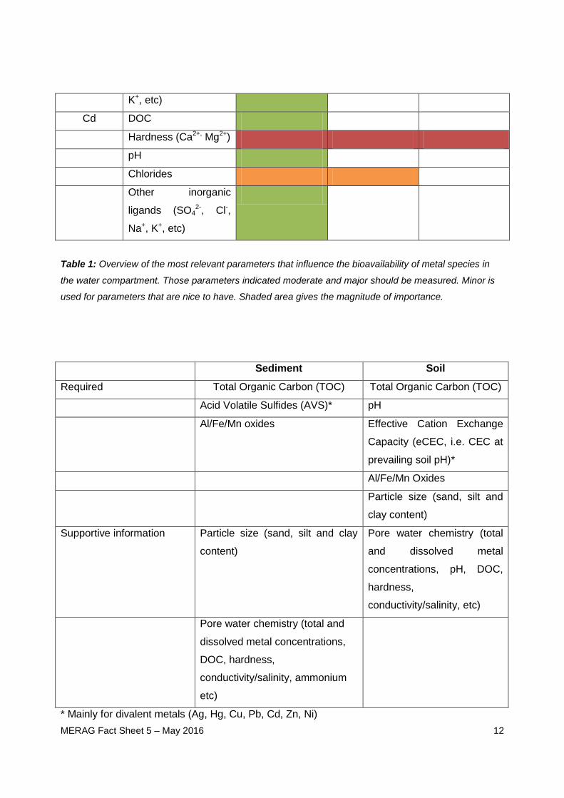
MERAG Fact Sheet 5 – May 2016
12
K+, etc)
Cd DOC
Hardness (Ca2+, Mg2+)
pH
Chlorides
Other inorganic
ligands (SO42-, Cl-,
Na+, K+, etc)
Table 1: Overview of the most relevant parameters that influence the bioavailability of metal species in
the water compartment. Those parameters indicated moderate and major should be measured. Minor is
used for parameters that are nice to have. Shaded area gives the magnitude of importance.
Sediment Soil
Required Total Organic Carbon (TOC) Total Organic Carbon (TOC)
Acid Volatile Sulfides (AVS)* pH
Al/Fe/Mn oxides Effective Cation Exchange
Capacity (eCEC, i.e. CEC at
prevailing soil pH)*
Al/Fe/Mn Oxides
Particle size (sand, silt and
clay content)
Supportive information Particle size (sand, silt and clay
content)
Pore water chemistry (total
and dissolved metal
concentrations, pH, DOC,
hardness,
conductivity/salinity, etc)
Pore water chemistry (total and
dissolved metal concentrations,
DOC, hardness,
conductivity/salinity, ammonium
etc)
* Mainly for divalent metals (Ag, Hg, Cu, Pb, Cd, Zn, Ni)

MERAG Fact Sheet 5 – May 2016
13
Table 2: Overview of the most relevant parameters that influence the bioavailability of metal species in
the sediment/soil compartment
The abiotic factors can be obtained from existing monitoring databases for a specific
region/area or from specific tailored monitoring campaigns (site specific). For a site-specific
assessment, quite often median concentrations are used. For setting thresholds that could be
used in a more cautious way, low or high concentrations (representative of realistic worst-case
conditions) of the abiotic factors should be selected.
Because the results of toxicity tests are also dependent on the bioavailability of the metal in the
test media, especially those conducted in natural media, measurements of abiotic factors in the
test medium should also be conducted. Furthermore, as metals are naturally occurring
substances, many organisms have evolved mechanisms to regulate the accumulation and
storage of these metals, which also influence their sensitivity towards these metals. This
phenomenon should ideally also be considered in selecting adequate ecotoxicity data for risk
assessment (see Factsheet 3). When test organisms have been cultured in conditions that are
outside the natural background concentration ranges, such data should be considered with care
and might even be discarded. It is, however, recognized that this may lead to a reduction in the
number of useful ecotoxicity data, which may even sometimes limit the possibility of using a
Species Sensitivity Distribution (SSD). Another complicating factor is that quite often culture
conditions are not reported. In that case, expert judgment should be used to decide if the study
can still be used or not.
In a regulatory context, metal exposure concentrations are typically compared to one single
numerical value in order to screen out potential risks (ie, in a risk assessment context) or to
identify non-compliance (in case of the use of Environmental Quality Standards/Guidelines,
Water Quality Criteria etc). Most often these values are expressed as total metal
concentrations. In implementing bioavailability, the purpose is to recalculate both exposure and
derived ecotoxicity thresholds to a metric that better reflects what an organism actually
“experiences” under certain environmental conditions. Hence the application of the
bioavailability concept to the water, sediment and soil compartment entails the normalisation of
MERAG Fact Sheet 5 – May 2016
14
conventional effect thresholds (for example, toxicity thresholds such as EC502, EC10, EC20),
expressed as total metal concentrations and exposure concentrations, using either soluble
fractions, speciation or bioavailability algorithms. The next three sections provide brief
descriptions of the tiered approaches and tools available to implement bioavailability for the
different compartments.
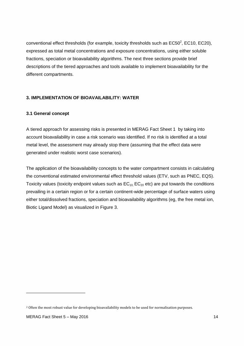
3. IMPLEMENTATION OF BIOAVAILABILITY: WATER
3.1 General concept
A tiered approach for assessing risks is presented in MERAG Fact Sheet 1 by taking into
account bioavailability in case a risk scenario was identified. If no risk is identified at a total
metal level, the assessment may already stop there (assuming that the effect data were
generated under realistic worst case scenarios).
The application of the bioavailability concepts to the water compartment consists in calculating
the conventional estimated environmental effect threshold values (ETV, such as PNEC, EQS).
Toxicity values (toxicity endpoint values such as EC10, EC20 etc) are put towards the conditions
prevailing in a certain region or for a certain continent-wide percentage of surface waters using
either total/dissolved fractions, speciation and bioavailability algorithms (eg, the free metal ion,
Biotic Ligand Model) as visualized in Figure 3.
2 Often the most robust value for developing bioavailability models to be used for normalisation purposes.
MERAG Fact Sheet 5 – May 2016
15
Figure 3: Refinement levels for the incorporation of bioavailability concept for the water compartment.
(Note total Me-concentration3 is only needed if information on the “Total dissolved” fraction
4 is not
available. The direct use of measured dissolved metal concentrations is preferred.)
3.2 Use of “total dissolved” metal
A rudimentary but not preferred way of taking into account (bio)availability, is the use of
dissolved concentrations. Translating a “total metal” concentration towards a “total dissolved
metal” concentration takes several physico-chemical phenomena into account. The dissolved
concentration of soluble metals (eg, Cu, Ni, Zn), under biologically relevant conditions, is mainly
driven by the adsorption onto suspended solids. In case of less soluble metals, the solubility of
the metals may be limited under specific environmentally relevant conditions (eg, Pb, Al, Fe,
Sn). For these metals, the dissolved metal concentrations will not only be driven by the
3 Total metal concentration and comprises particulate (sorbed + precipitated) + dissolved (inorganic complexes + organic complexes + free ionic forms). 4 Total dissolved metal concentration refers to the fraction that passes through a filter of 0.45 µm and comprises inorganic complexes + organic complexes + free ionic forms.
TOTAL METAL LEVELS (MONITORING DATA)
KD, SS
Ca, pH, DOC,… (speciation model)
Toxicity-based models (Biotic Ligand Model, Regression Models,…)
PHYSICO-CHEMICAL SPECIATION MODELLING
WATER
Total
Me-concentration
Free ionic
Me-fraction
Biogeochemical Regions X1, X2, Xn,…
Dissolved
Me-fraction
Bioavailable Metal Fraction
BIOAVAILABILITY ASSESSMENT MODELLING
KD, SS
TOTAL METAL LEVELS (MONITORING DATA)
KD, SS
Ca, pH, DOC,… (speciation model)
Toxicity-based models (Biotic Ligand Model, Regression Models,…)
PHYSICO-CHEMICAL SPECIATION MODELLING
WATER
Total
Me-concentration
WATER
Total
Me-concentration
Free ionic
Me-fraction
Biogeochemical Regions X1, X2, Xn,…
Dissolved
Me-fraction
Bioavailable Metal Fraction
BIOAVAILABILITY ASSESSMENT MODELLING
KD, SS

MERAG Fact Sheet 5 – May 2016
16
adsorption, If the solubility limit is exceeded, metal precipitation also plays an important role.
While for some metals the formation of solid precipitates will render the metal less toxic (eg,
lead), it has been observed for others that physical interaction between the precipitated metal
forms and the active sites on an organism may occur and subsequently may also contribute to
the observed toxicity. For example, several authors have suggested that polymerization or
precipitation of Al hydroxide at the gill may be responsible for observed respiratory effects in fish
(Playle and Wood 1989, 1990; Poleo 1995). However, it should be noted that the latter effects
could be transient in nature due to the use and disequilibrium of freshly prepared aluminium
solutions in toxicity tests.
Taking into account the different processes and metal forms that could occur in an ambient
water and/or test medium, the following operationally defined terms will be subsequently used to
make a distinction between “Total metal” and Total dissolved metal” :
Total metal concentration comprises particulate (sorbed + precipitated) + dissolved
(inorganic complexes + organic complexes + free ionic forms);
Total dissolved metal concentration refers to the fraction that passes through a filter of 0.45
µm and comprises inorganic complexes + organic complexes + free ionic forms.
It should be noted that the free ion is not necessarily the best predictor for the ecotoxicity of all
metals because other metal species (eg, AgCl, HgS) may contribute to the observed toxicity
(Campbell 1995).
The use of ambient and/or total dissolved metal concentrations to report ecotoxicity data and
the derivation of an environmental threshold value and risk ratio is done in the sequence as
outlined in Figure 4 and detailed in the text (steps 1-6 following the figure).

MERAG Fact Sheet 5 – May 2016
17
Figure 4: Framework for assessing risks of metals/metal compounds in water (sequence applies to both
the local and regional environment) on a dissolved basis. (Where Tox = ecotox value; C = environmental
concentration; PEC = predicted environmental concentration; SLa = solubility limit ambient; SLt =
solubility limit toxicity test; * = applies for sparingly soluble metals only.)
1. For soluble metals (ie, metals that occur in a dissolved fraction under
environmental relevant concentrations), the direct use of measured dissolved
concentrations is preferred.
2. If dissolved measured concentrations are not available and exposure data are
only expressed as total metal concentrations, the individual Ctotal concentrations
can be recalculated into C total, dissolved concentrations using Equation 1:
Ctotal, dissolved =Ctotal
(1+Kd ´Cs, a´10-6 ) (Eq-1)
Ctotal = total environmental concentration (mg/L)
Ctotal, dissolved = total dissolved environmental concentration (mg/L)
Kd = Partitioning distribution coefficient (L/kg)
Cs,a = Suspended solids concentration in the ambient water (mg/L)
3. In a similar way the total concentrations in toxicity tests (TOXtotal,)
concentrations are extrapolated into total dissolved concentrations in toxicity
tests (TOXtotal, dissolved) concentrations using Equation 2. Note that aquatic toxicity

MERAG Fact Sheet 5 – May 2016
18
tests tend to maximise metal availability because most often DOC levels are low
(< 2mg/L). Most toxicity tests are being conducted with reconstituted water and in
those cases no additional conversion to a dissolved fraction has to be applied (ie,
the total concentration can be set equal to the dissolved concentration5). If
natural waters are used, total concentrations should be recalculated using
partition coefficients.
TOXtotal, dissolved =TOXtotal
(1+Kd ´Cs, t´10-6 ) (Eq-2)
TOXtotal = total concentration in toxicity tests (mg/L)
TOXtotal, dissolved = total dissolved concentration in toxicity tests (mg/L)
Kd = Partitioning distribution coefficient (L/kg)
Cs,t = Suspended solids concentration in toxicity tests (mg/L)
In case precipitation occurs under specific environmentally relevant conditions and/or for
substances of very low solubility (<1mg/L), the toxicity data might need to be corrected by taking
the solubility limits of these metals into account. These solubility limits are mainly driven by
abiotic environmental factors (eg, pH, DOC) and could be estimated using specific speciation
models6 (eg, Visual MINTEQ, PHREEQC) or experimentally derived (Example 1).
5 It must be demonstrated that the organic particles (from eg, faeces and food) that appears in the test system do not
significantly affect the dissolved metal concentration in the test. Also surface adsorption could be the cause of decreased
metal concentrations.
6 Some specific speciation models allow estimating precipitation of metals (eg, Visual MINTEQ, PHREEQC) while others do
not have that capacity (eg, WHAM).

MERAG Fact Sheet 5 – May 2016
19
Example 1: Derivation EC10 values for solubility-limited metals: case study Pb
The solubility of lead is limited under specific environmentally relevant conditions. Its solubility
limit is mainly driven by abiotic environmental factors (eg pH, hardness and DOC) and can be
estimated using WHAM or Visual MINTEQ, Figure 1.1 shows an example of the translation of two
ecotoxicity values expressed as total lead concentrations to dissolved Pb concentrations taking
into account the actual solubility conditions occurring in the test.
4. Calculate the Environmental Exposure Concentration total dissolved (EECtotaldissolved)
for a predefined local or regional environment (high end value eg, 90th percentile
of the environmental concentration distribution)

MERAG Fact Sheet 5 – May 2016
20
5. From all available dissolved ecotoxicity threshold data, a cautious environmental
threshold value (ETV) is derived using assessment factor approaches (data-poor
metals) or statistical extrapolation methods7. The ETV is subsequently compared
to the modelled and/or measured exposure data equally expressed as dissolved
concentrations (Cfr step 2).
6. The potential environmental risks (RCR) for a regional or local environment are
subsequently calculated from the comparison between the local/regional
EECdissolved and the ETVtotal,dissolved generic (Equation 3).
RCR =EECdissolved
ETVtotal, dissolved, generic
(Eq-3)
In selecting an appropriate Kd value to be used in Eq-1 and Eq-2, it should be acknowledged
that Kd values cannot be considered as true constants and will vary as a function of the metal
loading and as a function of environmental characteristics such as pH (due to proton
competition for binding sites) and ionic strength. Subsequently, as metal, Kd values will show a
large degree of variability irrespective if equilibrium has been reached or not. The assessment
of the data quality and relevance of all collected measured Kd values should be done with care.
Ranges spanning different orders of magnitude have been reported in the literature (Allison and
Allison 2005). (Allison ref is missing.) Preference should always be given to measured data for
which synoptic information is available on both sampling and analytical measuring techniques. If
only a limited data set of Kd values is available (less than 4 data points), the choice of the
appropriate Kd value should be based on expert judgment taking into account the
representativeness of the Kd value for the site/region of interest. The minimum and maximum
values can be used for the uncertainty analysis. For data-rich metals, sufficient Kd values can
be a log-normal distribution or another significant statistical distribution can be fitted through the
data points. The median Kd value can subsequently be used in the exposure and effects
assessment. An additional uncertainty analysis with a range of Kd values (eg, 10-90th
percentiles) is recommended.
7 For a large data set of toxicity data for one species the geomean is taken, but in case of a small data set most often there
is preference for selecting the most sensitive value rather than using a geomean value.

MERAG Fact Sheet 5 – May 2016
21
3.3 Use of “dissolved metal species of concern (DMSC)”
In cases where appropriate (externally validated) speciation models (eg, WHAM, visual
MINTEQ, CHESS, PHREEQC etc) and relevant input data on the main physico-chemical
parameters driving the availability of a metal are available, the risk characterisation should be
performed on the basis of the dissolved metal species of concern. Most often the dissolved
metal species of concern equals the free metal ion. Free ion activities can be directly measured.
However, the free metal ion is not necessarily the best predictor for all metals and other metal
species such as neutral species (eg, AgCl, HgS) and anionic species (eg, SeO2-, AsO42-) may
contribute to the observed toxicity (Campbell 1995) and are captured in this term. Instead of
measuring free ion activities, chemical speciation models are more often used to try to
accurately predict the distribution of an element amongst chemical species in an environmental
system. It should be noted that depending on which speciation model is used and which
parameter is the most influential, different speciation models might give different answers.
Speciation modelling is often needed as direct measurement techniques predominantly focus
on the quantification of the free metal ion concentrations, and even this approach is not always
possible at environmentally low concentrations. The outcome of speciation models may vary
and are sensitive to the selection of parameters that are included. Some of the reported
uncertainties are (Van Briesen et al 2010): decision rule uncertainty, model uncertainty,
parameter uncertainty, and parameter variability (Finkel 1990; Hertwich et al 1999). Therefore,
only validated and justified models for the metals under scrutiny should be used (eg, in Biotic
Ligand Model development). Sensitivity analysis could be a valuable tool in this context to
provide reassurance that any adopted approach is sufficiently precautionary. Further
harmonisation of speciation models is warranted in the future and existing speciation models
are currently modified in an attempt to further improve their predictive capacity.
A non-exhaustive overview of some recent models or model versions that can be used to
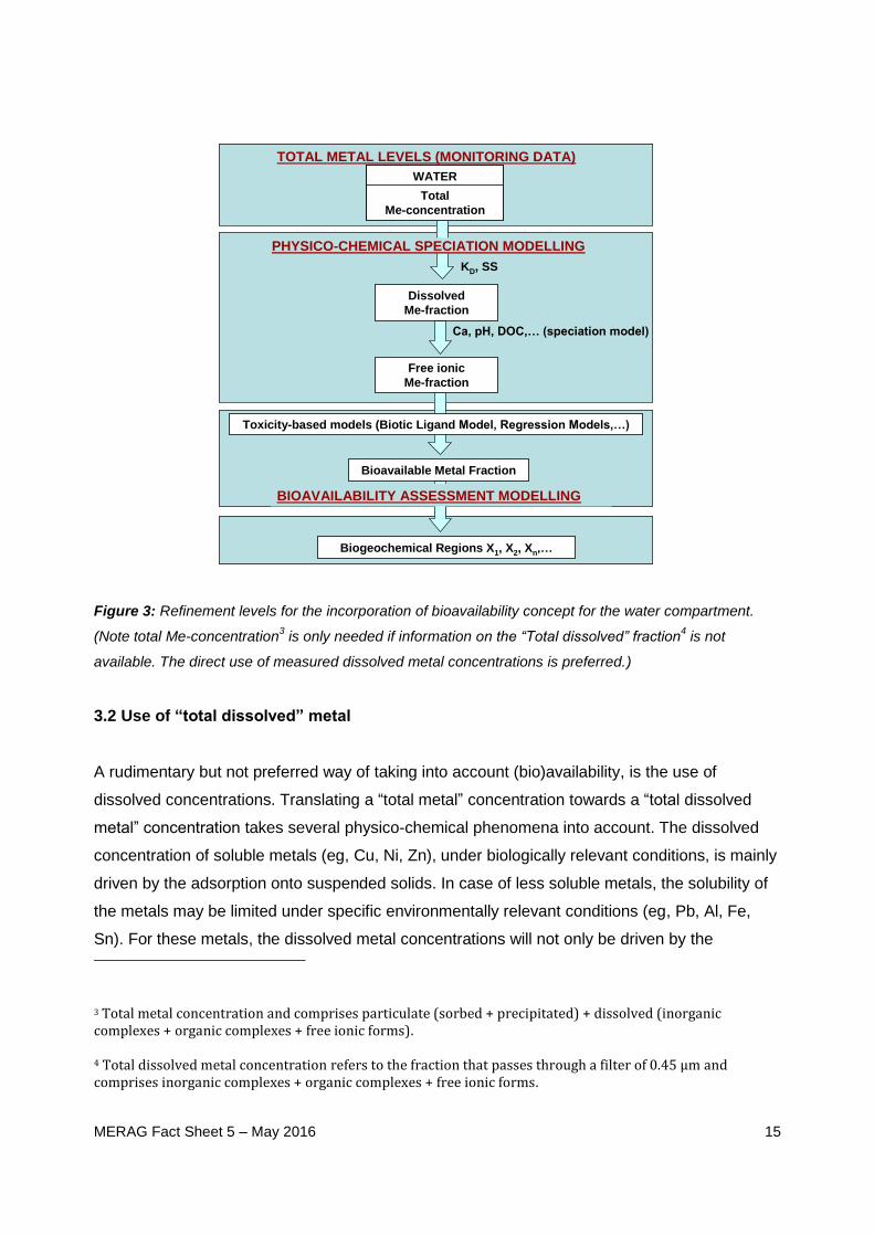
determine metal speciation is provided in Table 3.
Model More information on model
CHEAQS Next - CHemical Equilibria in AQuatic
Systems.
http://www.cheaqs.eu/
MERAG Fact Sheet 5 – May 2016
22
This model is the successor of the models GECHEQ and
CHEAQS Pro (developed by Wilko Verweij).
Calculation of the concentration of complexes
Complexation by natural organic matter (3
different models developed by Tipping and co-
workers: Model V, Model VI and Model VII;
Formation of solids due to oversaturation
Includes a surface complexation model to cover
adsorption processes).
ChemEQL
Determination of thermodynamic equilibrium
concentrations of species in complex chemical systems.
Adsorption on upto five different particulate
surfaces can be modelled
Simulations of kinetic reactions with one rate-
determining process
Calcluation of two-dimensional logarithmic
diagrams, (eg, pe-pH)
ChemEQL is an extended and user-friendly version of
the original program MICROQL. It runs on MacOSX,
Windows, Linux, and Solaris.
http://www.eawg.ch/research
MINTEQA2, version 4.03
A chemical equilibrium model for the calculation of metal
speciation, solubility equilibria etc, for natural waters.
Ion speciation using equilibrium constants (based
on the most recent NIST data)
Solubility calculation involving solid phases
Adsorption calculations with adsorption
isotherms, based on five surface complexation
models (Diffuse Layer, Constant Capacitance,
Triple Layer, Basic Stern and Three Plane)
Ion-exchange processes covered (Gaines-
Thomas formalism)
Metal-humic complexation can be simulated
http://www2.epa.gov/exposur
e-assessment-
models/minteqa2

MERAG Fact Sheet 5 – May 2016
23
using the Gaussian DOM, the Stockholm Humic
Model, or the NICA-Donnan model
Visual MINTEQ is a Windows version of
MINTEQA2 v.4.0
PHREEQC (Version 2): A computer program for
speciation, batch-reaction, one-dimensional transport,
and inverse geochemical calculations
Written in the C programming language that is
designed to perform a wide variety of low-
temperature aqueous geochemical calculations
Transport calculations involving reversible and
irreversible reactions
Windows, Linux and MacOS versions are
available
http://wwwbrr.cr.usgs.gov/pro
jects/GWC_coupled/phreeqc/
WHAM 7 – Windermere Humic Aqueous Model,
version 7
Model for the calculation of equilibrium chemical
speciation in surface and ground waters, sediments and
soils (developed by E.Tipping and colleagues?).
Suitable for problems where the chemical
speciation is dominated by organic matter
Model takes into account the precipitation of
aluminium and iron oxides, cation-exchange on
an idealized clay mineral, and adsorption-
desorption reactions of fulvic acid
Ion accumulation in the diffuse layers
surrounding the humic molecules is considered
Model calculations are performed with a BASIC
computer code running on a Personal Computer.
https://www.ceh.ac.uk/servic
es/software-models
Table 3: Overview of frequently used chemical speciation models (source: www.speciation.net)
It is important to know, however, that some of the speciation models that were used for the
development of BLMs – or that are even incorporated into their software -- do not always
represent the most current version. An overview of some of the models that have been used for

MERAG Fact Sheet 5 – May 2016
24
BLM-purposes are shown in Table 4. The choice for using a specific speciation model for a
metal for modelling the dissolved species of concern, and in particular the interaction between
metals and (dissolved) organic carbon, has been made for various reasons such as the state-of-
the-art at the time of the Biotic Ligand Models development, or functionalities of the speciation
model that meet the needs for a specific metal. Different speciation models are used for
different metals: WHAM 5 (Cu, Zn, Co), WHAM 6 (Ni), Visual MINTEQ V3 (Pb) (Table 4).
Speciation Model Metals for which
the speciation
model is used
Rationale
Windermere Humic
Aqueous Model, Version
V (WHAM 5)
Copper
(Hydroqual,
UGent Model)
Zinc
Cobalt
WHAM 5 model was originally used in the
development of the first copper and silver
BLM by HydroQual/HDR, and was
subsequently used in the development of the
BLMs for zinc and copper by Ghent
University. The cobalt BLM (HydroQual/HDR)
was also developed with this version of
WHAM
Windermere Humic
Aqueous Model, Version
VI (WHAM 6)
Nickel Initial modeling of nickel speciation with
WHAM 5 resulted in poor predictions at low
nickel concentrations. The use of the
upgraded WHAM-6 model significantly
improved predictive capacity of the BLM. The
WHAM-6 model also allowed users to make
adaptations to eg, the binding and stability
constants of metal (compounds) to organic
carbon (fulvic acid and humic acid).
Visual MINTEQ version
3.0 (code built on
MINTEQA2; optimized
for metal complexing
effects of DOM)
Lead This model allowed a proper description of
Pb-speciation with the NICA-Donnan model,
and this was also the only speciation model
at the time of development that took both Pb-
precipitation as well as binding of Pb to
organic material into account.
.

MERAG Fact Sheet 5 – May 2016
25
Table 4: Rationale and overview speciation models used for translating total dissolved concentrations to
total dissolved metal species of concern
MERAG Fact Sheet 5 – May 2016
26
If there is a concern that the investigated metal binds strongly on colloids, this should ideally be
considered in calculating the speciation of dissolved metal because colloids can pass through
most filters and if ignored may have an impact on the overall outcome of the speciation
exercise. However, at the moment, our understanding on colloids is limited and further research
is needed in this field before this could be embedded in speciation calculations.
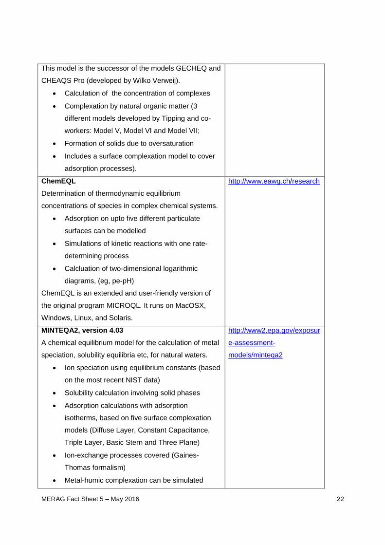
Figure 5 gives an overview of the proposed tiered approach.
Figure 5 Framework for assessing risks of metals/metal compounds in water on a free metal ion basis.
(Where Tox = ecotox value; C = environmental concentration; * = sequence applies to both the local and
regional environment.)
7. It is recommended to recalculate the reported total dissolved TOX concentrations
(TOX total dissolved) into Tox concentrations expressed as the metal species of
concern (TOXdissolved metal species of concern) using the appropriate speciation models
(eg, PHREEQC, WHAM, Visual MINTEQ,…) and taking into account the main
physico-chemical conditions driving the bioavailability (eg, pH, DOC,…) of the
individual toxicity test result (ie, for a specific test species and for the metal
compound in question). If no specific information on relevant physico-chemical
parameters is available, then the toxicity data should not be used unless the

MERAG Fact Sheet 5 – May 2016
27
possibility of using default values instead can be substantiated. For example, for
copper, Santore et al (2001) used a default DOC value of 1 mg/L to calibrate the
acute copper BLM.
8. It is recommended to recalculate the total dissolved exposure concentrations
(Ctotal disssolved) at the same level of bioavailability (expressed in the same units) as
that used to recalculate the TOX concentrations, ie, into metal species of concern
exposure concentrations using the same speciation model (eg, PHREEQC,
WHAM, Visual MINTEQ,…). For that purpose, the physico-chemical parameters
of the generic environment or site-specific watershed driving the bioavailability
(eg, pH, DOC,…) should be gathered or estimated. Reference is given to either
realistic worst case (eg, 10th/90th percentile) or typical conditions (eg, 50th
percentile), depending on the regulatory setting in which these values are used.
9. From all available Tox dissolved metal species of concern ecotoxicity threshold data, a
cautious environmental threshold value (ETV) is derived and compared to the
Environmental Exposure Concentration metal species of concern derived from all
individual Cdissolved metal species of concern values for a predefined environment taking a
high end value (eg, the 90th percentile) of the environmental concentration
distribution of the metal species of concern.
10. The risks for a local or regional environment are subsequently calculated from
the comparison between the EECdissolved metal species of concern and the ETV dissolved metal
species of concern (Equation 4):
RCR =EECmetalspeciesofconcern
ETVmetalspeciesofconcern (Eq-4)
Example 2: Use of dissolved metal species of concern.
For highly soluble metals such as Cu or Zn, the difference between total and dissolved (filtered)
metal concentration is expected to be small in most surface waters and ecotoxicity test media.
But in the case of a poorly soluble metal such as lead, this difference can be substantial. Lead
and its compounds will show indeed a low solubility under typical ecotoxicity testing, particularly
at higher pH and alkalinity levels where lead carbonate and lead hydroxide minerals often tend to
precipitate from exposure media (Kopittke et al 2008). But also other parameters of the receiving
water (eg, DOC, hardness) may have an important influence on the aquatic toxicity of lead.
Recently, for lead a DOC-based regression has been proposed for the aquatic EQS derivation in
the context of the EU Water Framework Directive (EQS-TGD (2011). The process entailed the
determination of significant relationships between DOC and chronic lead toxicity for different

MERAG Fact Sheet 5 – May 2016
28
freshwater species (Cerodaphnia dubia, Pimephales promelas, Lemna minor, Pseudokirchienella
subcapitata, Philodina rapida and Limnea stagnalis). The most conservative slope of the equation
(ie, 1.2) was found for the rotifer P. rapida (Esbaugh et al 2012) and used to calculate the HC5-
50reference based on the selection of chronic lead toxicity data with low DOC (ie, 1 mg/L on
average). Subsequently the HC5-50 for a specific site can be calculated with the following
equation:
HC5-50site = HC5-50reference + (1.2 x (DOCsite –DOCreference)
3.4 Development and application of toxicity- related bioavailability models
3.4.1 General outline
Preferentially, the assessment should be performed on a „bioavailable‟ basis. For this purpose,
ambient dissolved metal concentrations and appropriate toxicity-related bioavailability models
(eg, Biotic Ligand Model) could be used. The conceptual part of the Biotic Ligand Model (BLM)
can be considered in terms of three separate components. The first component involves the
solution chemistry in the bulk water, which allows prediction of the concentration of the toxic
metal species. These chemical speciation computations are standard and can be performed
with any of the several speciation models that exist. A second component involves the binding
of the toxic metal species to the biotic ligand. The final component is the relationship between
the metal binding to the biotic ligand and the toxic response. The presence of the biological
component (ie, binding to the metal binding sites within an organism) suggests that the
bioavailability correction should conceptually be applied on the effects side of the equation.
However, for regulatory purposes, it could equally be applied at the exposure side using the
Bio-F approach.
Figure 6 presents the stepwise procedure when using the BLMs in the assessment of metals
and is described in further detail below. In comparing the environmental concentrations and the
effect concentrations, care should be taken that both are expressed in the same units.

MERAG Fact Sheet 5 – May 2016
29
Figure 6: Framework for incorporation of bioavailability models for the water compartment. Where X =
test conditions; Y = reasonable worst-case conditions or typical conditions (depending on the scenario); H
= hardness; DOC = dissolved organic carbon.
Step 1: Determine the critical biotic ligand accumulation (TOXcritical biotic ligand, organism xi) calculated
from the organism specific toxicity values (TOXdissolved, organism xi), expressed as dissolved
concentration. Organism-specific bioavailability models should be used as much as possible for
that purpose (see section 3.4.3 on cross-species extrapolation for further guidance).
Step 2: Recalculate each organisms specific critical biotic ligand binding (TOXcritical biotic ligand,
organism xi) into a critical bioavailable dissolved concentration (TOX(critical bioavailable dissolved)y, organism xi)
for a specific area under investigation, characterised by a specific set of water-quality conditions
(pHy, Hy, DOCy).

MERAG Fact Sheet 5 – May 2016
30
Step 3: Use the critical bioavailable dissolved concentrations (Tox(critical bioavailable dissolved)y, organism xi)
to derive a cautious environmental threshold value (ETV) using assessment factor approaches
(data poor metals) or statistical extrapolation methods. This value is subsequently compared to
the selected modelled and/or measured environmental exposure concentration (EEC) equally
expressed as dissolved concentrations. The EEC is calculated from all individual Cdissolved values
for a predefined environment taking a high end value (eg, the 90th percentile) of the
environmental concentration distribution of the metal species of concern.
In the context of a generic risk assessment and/or compliance checking, the BLM models can
be used to convert the effects data to well-characterised specific local or regional conditions (ie,
establishing ETVlocal, bioavailable or ETVregional, bioavailable) or reasonable worst case conditions (ie,
establishing ETVreference, bioavailable) .
Conceptually, the BLM framework is a valid descriptor of metal bioavailability when toxicity is a
result of exposure to the dissolved metal ion. It should, however, be noted that for some metals,
combined toxicity effects due to both the dissolved and precipitated metal forms have been
demonstrated under specific environmental conditions (eg, aluminium). For those cases the
mechanistic BLM framework needs to be extended to account for the additional physical effects
due to the interaction between precipitated forms and the biotic ligand. Furthermore, as BLM
models are developed for a well-defined chemical (abiotic factors) and toxicological data set
that define their validated application boundaries, it should be evaluated if the local water
chemistry falls within the BLM application domain. If not, this does not immediately prohibit the
use of the model. For example, if for increasing pH values (6-8), the BLM predicts less toxicity
than the upper pH limit of the BLM (ie, 8), it could be used as a conservative estimate for
toxicity. The BLM model should, however, not be used in the other direction when toxicity would
increase. In that case, it should just be flagged that the water chemistry falls outside the
boundaries. Eventually, spot checks can be used to verify if the model could be extended into
that region.
Table 5 gives a non-exhaustive overview of several acute and chronic aquatic BLMs/screening
tools that are reported in the literature. It should be noted that it is unknown if all BLMs have
been properly validated (see section 3.4.2). The relevance for developing a BLM could be
compartment specific (eg, a BLM for Mo was not developed for water because of its very low
toxicity for the aquatic compartment, but bioavailability models were developed and deemed
relevant for soil).

MERAG Fact Sheet 5 – May 2016
31
Metal Available acute BLMs - main relevant publications
Most BLMs have been developed for regulatory purposes. Environmental risk
assessments are predominantly driven by long-term effects (chronic toxicity), and
therefore most BLM tools focussed on chronic endpoints. There are, however, a large
number of publications on acute toxicity-based BLMs. This work, however, was not
always translated into the development of user-friendly and publicly-accessible acute
BLM tools/models.
With regard to acute BLMs, this table only provides the most relevant references that
report on key BLM parameters (ie,binding constants). Additional references (eg,
publications that only focus on the metal-gill binding interaction) can be found in
Ardestani et al (2014).
Ag Bury et al 2002; Janes and Playle 1995; McGeer et al 2000; Morgan and Wood
2004; Paquin et al 1999.
As Chen et al 2009.
Cd Clifford and McGeer 2010; Francois L et al 2007; Hatano and Shoji 2008;
Hollis et al 2000; Janssen et al 2002; Niyogi et al 2004/2008; Playle et al 1993;
Rachou and Sauve 2008; Schwartz et al 2004; Van Ginneken et al 1999.
Co Richards and Playle 1998.
Cu Brooks et al 2006; Constantino et al 2011; De Schamphelaere and Janssen
2002; De Schamphelaere et al 2007; Di Toro et al 2001; Ferreira et al 2009;
Gheorghiu et al 2010; Hatano and Shoji 2008/2010; MacRae et al 1999; Meyer
et al 2007; Playle et al 1993; Rachou and Sauve 2008; Ryan et al 2009;
Santore et al 2001; Taylor et al 2003; Villavicencio et al2011; Welsh et al 2008.
Hg Klinck et al 2005.
Pb MacDonald et al 2002; Schwartz et al 2004; Slaveykova and Wilkinson 2003.
Mn Francois et al 2007; Peters et al 2011.
Ni Deleebeeck et al 2007a,b/2008/2009a,b; De Schamphelaere et al 2006; Keithly
et al 2004; Kozlova et al 2009; Worms and Wilkinson 2007; Wu et al 2003.
U Fortin et al 2007.
Zn Alsop and Wood 2000; Clifford and McGeer 2009; De Schamphelaere and
Janssen 2004; Heijerick et al 2002a,b; Santore et al2001/2002; Schwartz et al
2004; Todd et al 2009; Van Ginneken et al 1999.
Metal Available chronic BLMs (driving Reference/link

MERAG Fact Sheet 5 – May 2016
32
abiotic factor)
It should be noted that pH is not always specifically included as driving abiotic factor, but
is only mentioned when specific binding constants for H+ have been derived. Impact of
pH, however, is often indirectly included in the speciation calculation.
Ag Silver: bioavailability effects due to
DOC and sulphide (expressed as
Chromium Reducible Sulphide (CRS)
Silver will be toxic under conditions
where the molar concentration of Ag
exceeds the molar concentration of
CRS (cfr SEM/AVS approach for
metals in sediment)
www.hydroqual.com/wr_blm.html
Cd Predominantly competition with major
(hardness) cations
www.hydroqual.com/wr_blm.html
Cu Predominantly DOC-effect, some
competition with major cations
www.pnec-pro.com
bio-met.net
www.hydroqual.com/wr_blm.html
http://www.wfduk.org/resources/rivers-
lakes-metal-bioavailability-
assessment-tool-m-bat
Pb Clear effect of DOC on toxicity, but
speciation complicated by
precipitation with phosphate
www.leadblm.com
www.hydroqual.com/wr_blm.html
http://vminteq.lwr.kth.se/
Ni Effects from both DOC and
competing ions
www.pnec-pro.com
bio-met.net
www.hydroqual.com/wr_blm.html
http://www.wfduk.org/resources/rivers-
lakes-metal-bioavailability-
assessment-tool-m-bat
Mn Evidence of a protective effect from
hardness – chronic BLM
development
Competition from Ca2+ for fish and
invertebrates, and competition from
http://www.wfduk.org/resources/rivers-
lakes-metal-bioavailability-
assessment-tool-m-bat
MERAG Fact Sheet 5 – May 2016
33
H+ for algae
Limited effect of DOC (limited binding
of Mn)
Zn Effects from both DOC and
competing ions
www.pnec-pro.com
bio-met.net
www.hydroqual.com/wr_blm.html
http://www.wfduk.org/resources/rivers-
lakes-metal-bioavailability-
assessment-tool-m-bat
Table 5: Overview acute and chronic BLMs
3.4.2 Validation of BLM models
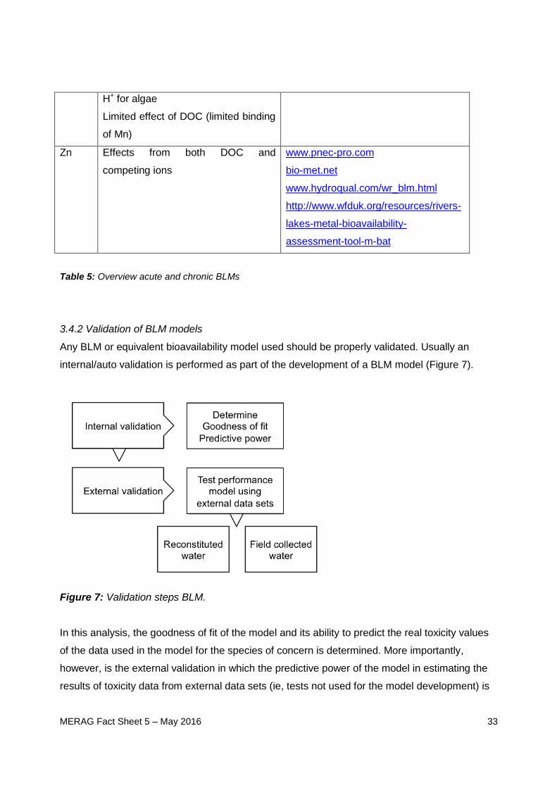
Any BLM or equivalent bioavailability model used should be properly validated. Usually an
internal/auto validation is performed as part of the development of a BLM model (Figure 7).
Figure 7: Validation steps BLM.
In this analysis, the goodness of fit of the model and its ability to predict the real toxicity values
of the data used in the model for the species of concern is determined. More importantly,
however, is the external validation in which the predictive power of the model in estimating the
results of toxicity data from external data sets (ie, tests not used for the model development) is

MERAG Fact Sheet 5 – May 2016
34
evaluated. These tests should be conducted in lab-reconstituted and/or field-collected natural
waters with a range of abiotic parameters overarching the applicability domain of the BLM.
If a BLM is validated, it can be used to normalise single ecotoxicity data or the different data
points of a species sensitivity distributions towards the condition prevailing in a region and/or
local site (example 3).
Example 3: Application of Cu BLM normalisations towards different biogeochemical
regions
The chronic BLM models have been applied to a set of biogeochemical regions used as
examples in the different EU metal risk assessments. For this exercise each organism- specific
critical biotic ligand accumulation [Cu] biotic ligand critical is translated into a critical bioavailable
dissolved concentration [Cu] bioavailable, dissolved for the area under investigation characterised by a
specific set of water-quality conditions (DOC, hardness and pH). Using the chronic BLMs will
finally result in the derivation of different Species Sensitivity Distributions (SSDs) and EQS values
for the different biogeochemical regions. The water chemistry and median HC5 values calculated
for the different selected biogeochemical regions in EU-surface waters are summarised in Table
3.1.
Table 3.1: Overview of the water chemistry and median HC5 values for the different EU
eco-regions
Biogeochemical
region
Water chemistry Median HC5
(best fit) (µg/L)
Median
HC5
(log normal)
(µg/L)
Ditch (The
Netherlands)
pH 6.9, H 260 mg/L, DOC 12.0
mg/L
22.1 27.2
River Otter (UK) pH 8.1, H 165 mg/L, DOC 3.2
mg/L
7.8 7.8
River Teme (UK) pH 7.6, H 159 mg/L, DOC 8.0
mg/L
17.6 21.9
River Rhine (The
Netherlands)
pH 7.8, H 217 mg/L, DOC 2.8
mg/L
8.2 8.2
River Ebro (Spain) pH 8.2, H 273 mg/L, DOC 3.7
mg/L
9.3 10.6
Oligotrophic Lake
Monate (Italy)
pH 7.7, H 48.3 mg/L, DOC 2.5
mg/L
10.6 10.6
Acidic lake (Sweden) pH 6.7, H 27.8 mg/L, DOC 3.8 11.5 11.1
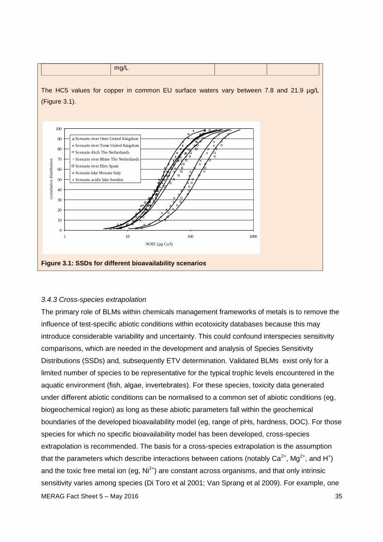
MERAG Fact Sheet 5 – May 2016
35
mg/L
The HC5 values for copper in common EU surface waters vary between 7.8 and 21.9 µg/L
(Figure 3.1).
Figure 3.1: SSDs for different bioavailability scenarios
3.4.3 Cross-species extrapolation
The primary role of BLMs within chemicals management frameworks of metals is to remove the
influence of test-specific abiotic conditions within ecotoxicity databases because this may
introduce considerable variability and uncertainty. This could confound interspecies sensitivity
comparisons, which are needed in the development and analysis of Species Sensitivity
Distributions (SSDs) and, subsequently ETV determination. Validated BLMs exist only for a
limited number of species to be representative for the typical trophic levels encountered in the
aquatic environment (fish, algae, invertebrates). For these species, toxicity data generated
under different abiotic conditions can be normalised to a common set of abiotic conditions (eg,
biogeochemical region) as long as these abiotic parameters fall within the geochemical
boundaries of the developed bioavailability model (eg, range of pHs, hardness, DOC). For those
species for which no specific bioavailability model has been developed, cross-species
extrapolation is recommended. The basis for a cross-species extrapolation is the assumption
that the parameters which describe interactions between cations (notably Ca2+, Mg2+, and H+)
and the toxic free metal ion (eg, Ni2+) are constant across organisms, and that only intrinsic
sensitivity varies among species (Di Toro et al 2001; Van Sprang et al 2009). For example, one
0
10
20
30
40
50
60
70
80
90
100
1 10 100 1000
NOEC (µg Cu/l)
cu
mu
lati
ve d
istr
ibu
tio
n
Scenario river Otter United Kingdom
Scenario river Teme United Kingdom
Scenario ditch The Netherlands
Scenario river Rhine The Netherlands
Scenario river Ebro Spain
Scenario lake Monate Italy
Scenario acidic lake Sweden

MERAG Fact Sheet 5 – May 2016
36
possibility is to implicitly assume that BLMs can be extrapolated within taxonomically similar
groups, ie, that BLMs developed for the rainbow trout O.mykiss can be applied to ecotoxicity
data for other fish species, that BLMs for D. magna/C. dubia can be applied to ecotoxicity data
for other invertebrates, and that BLMs for the green alga P. subcapitata can be applied to
ecotoxicity data for other algae. This assumption can be supported by quantitative evidence
showing that the available chronic BLMs can even predict toxicity for taxonomically dissimilar
species with reasonable accuracy (Schlekat et al 2010). In any case, if cross-species
extrapolation is used within dissimilar taxonomic groups, it should be verified on a case-by-case
basis using spot checks if observed versus the predicted toxicity values fall within a factor of 2.
It should be noted that normalisation using bioavailability models (eg, BLM) and cross-species
extrapolation to other species for which no bioavailability model is available applies to any
compartment where a bioavailability model is available.
Depending on the number of validated BLMs available per trophic level, a full-read cross-
species extrapolation, a reasonable worst case (RWC) cross-species extrapolation or no BLM
correction can be applied (Figure 8).
Figure 8: Approach for cross-species extrapolation of bioavailability models.
In order to extrapolate across species in all typical trophic levels
(algae/fish/invertebrates) a validated BLM should be available at least for each level.

MERAG Fact Sheet 5 – May 2016
37
The applicability of the bioavailability model across species can be assessed by
comparing information on the mechanism of action (MOA) of the metal under
consideration for the different species. If the MOA is different between two species, the
BLM should not be used. Another criterion for application is the extent in which the BLM
models can reduce the intra-species variability. This intra-species variability can be
assessed by comparing the predicted vs. observed toxicity for the different species or by
means of the max/min ratio between toxicity thresholds. If it can be demonstrated that
the interspecies variability is significantly decreased (ie, min-max ratio is smaller after
normalisation), the bioavailability model can be used across species.
These so-called spot checks consist typically of relatively few ecotoxicity tests,
performed with species for which the BLM will be applied under different geochemical
conditions for a range of key bioavailability parameters (eg, pH & DOC). Considering
that sensitive species are driving the ETV derivation, it should further be demonstrated
that the developed/validated bioavailability models can be applied to the most sensitive
species/taxonomic groups. For nickel, in addition to the 3 trophic levels (algae, fish and
daphnids), an additional species-specific BLM was developed for the daphnid
Ceriodaphnia dubia. In case of a local assessment where endemic species may require
specific protection, the models should be equally protective for the typical endemic
species of the database (Example 4).
In case cross-species extrapolation is only justified for some species and not for others
(eg, unexplained significant increase in variability after normalisation, different mode of
action or no spot checks available to justify extrapolation to dissimilar taxonomic
groups/trophic levels), an alternative more precautionary cross-species extrapolation
approach should be applied. In this RWC approach, the bioavailability models are only
applied to those species within the trophic level for which the application can be justified.
For those species for which application of the bioavailability model cannot be justified, a
bioavailability factor based on the most conservative available bioavailability model
should be applied.
Conceptually, the BLM developed for aquatic animals are related to toxicity caused by
uptake through gills, although the concept seems to work for gill-less organisms too. The
relative importance of dietary exposure is discussed further in this document.
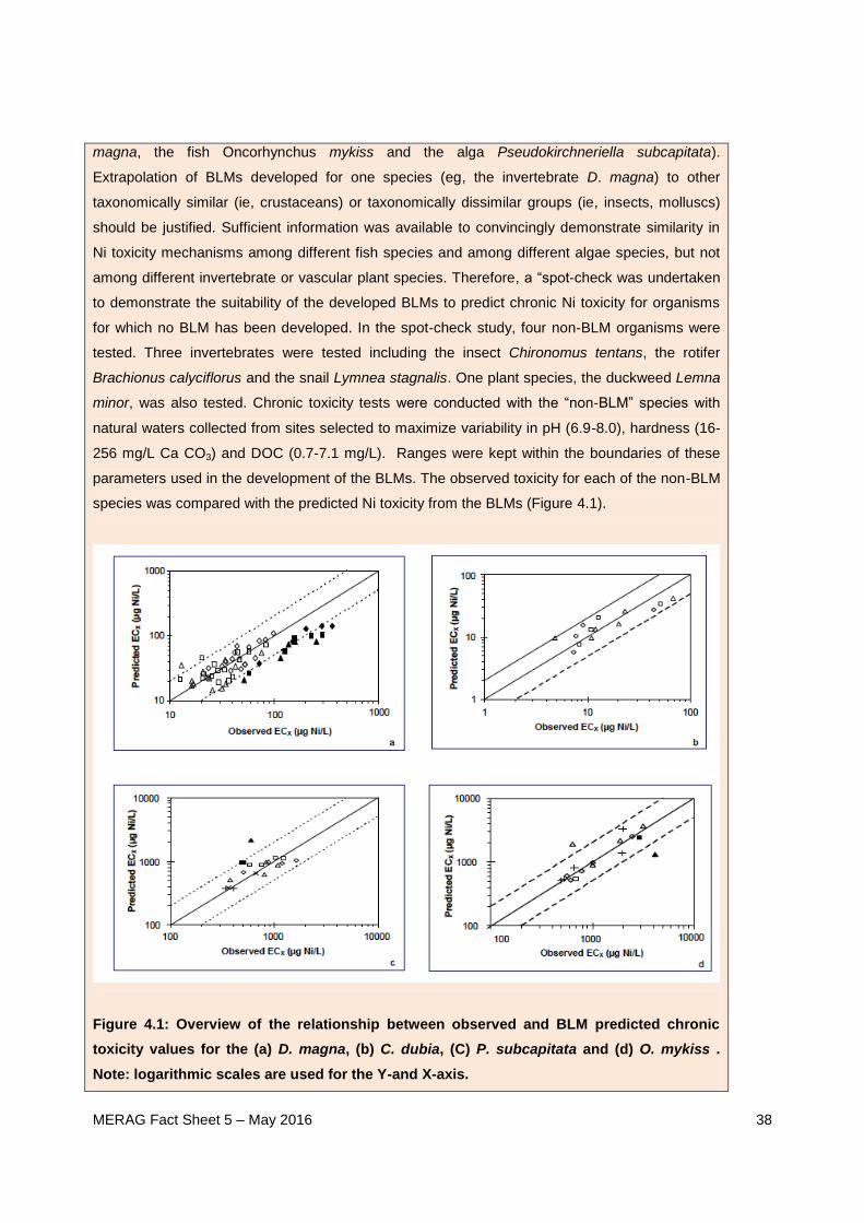
Example 4: Justification cross-species extrapolation using spot checks
The chronic Ni aquatic toxicity database contains data for 31 species while fully validated chronic
Ni BLMs are available for only 4 species (ie, the invertebrates Ceriodaphnia dubia and Daphnia
MERAG Fact Sheet 5 – May 2016
38
magna, the fish Oncorhynchus mykiss and the alga Pseudokirchneriella subcapitata).
Extrapolation of BLMs developed for one species (eg, the invertebrate D. magna) to other
taxonomically similar (ie, crustaceans) or taxonomically dissimilar groups (ie, insects, molluscs)
should be justified. Sufficient information was available to convincingly demonstrate similarity in
Ni toxicity mechanisms among different fish species and among different algae species, but not
among different invertebrate or vascular plant species. Therefore, a “spot-check was undertaken
to demonstrate the suitability of the developed BLMs to predict chronic Ni toxicity for organisms
for which no BLM has been developed. In the spot-check study, four non-BLM organisms were
tested. Three invertebrates were tested including the insect Chironomus tentans, the rotifer
Brachionus calyciflorus and the snail Lymnea stagnalis. One plant species, the duckweed Lemna
minor, was also tested. Chronic toxicity tests were conducted with the “non-BLM” species with
natural waters collected from sites selected to maximize variability in pH (6.9-8.0), hardness (16-
256 mg/L Ca CO3) and DOC (0.7-7.1 mg/L). Ranges were kept within the boundaries of these
parameters used in the development of the BLMs. The observed toxicity for each of the non-BLM
species was compared with the predicted Ni toxicity from the BLMs (Figure 4.1).
Figure 4.1: Overview of the relationship between observed and BLM predicted chronic
toxicity values for the (a) D. magna, (b) C. dubia, (C) P. subcapitata and (d) O. mykiss .
Note: logarithmic scales are used for the Y-and X-axis.

MERAG Fact Sheet 5 – May 2016
39
Results showed that the BLMs were able to accurately predict Ni toxicity to the spot check
species (Schlekat et al 2010). Based on the results from the spot check exercise and other weight
of evidence arguments (ie, the ecological relevance of the BLMs, accuracy of the BLMs and the
conservatisms of the proposed cross-species approach), the following final normalisation
approach was determined to be appropriate for the standardization of Ni toxicity data.
1. The P. subcapitata BLM can be used to normalise the chronic toxicity to other
algae,
2. The O. mykiss BLM can be used to normalise the chronic toxicity to fish and
amphibians,
3. For cladocerans, insects and amphipods, the most stringent result of the D.
magna, and C. dubia BLMs can be used, and
4. For rotifers, the D. magna BLM can be used and, for the invertebrates molluscs
and hydra, the C. dubia (best fitting BLM) can be used.
Because it is expected that the mechanism of toxicity between short- and long-term exposures
may differ, the use of acute bioavailability models to normalize chronic data should be
considered with great care8. Such normalisation is only allowed in case the predictive capacity
of these acute models for estimating chronic toxicity data is sufficient. In case of poor predictive
power of the acute models towards chronic toxicity data, the acute model could only be used to
normalise the acute toxicity data. The derivation of chronic effects levels could then be derived
from the normalised acute toxicity data using an acute to chronic ratio.
The complete bioavailability normalisation procedure using cross-species extrapolation is
illustrated below in further details to a reference scenario (eg, reasonable worst case conditions
or RWC) but could equally be adapted to a specific local and/or regional scenario, respectively.
8 Both acute (eg Cu, Ni, Pb, Zn, Ag, Co etc Al according to Adams and Santore? …) and chronic (ie Zn, Cu, Ni, Pb) BLMs for
metals have been developed/validated and proposed for regulatory purposes, both for environmental risk assessment
exercises and for the development of site-specific water quality criteria. More details on the development, application and
restrictions of using BLMs can be found in eg, Bossuyt et al (2004); Deleebeeck et al (2006, 2007a/b, 2008a/b/c); De
Schamphelaere (2003); De Schamphelaere and Janssen (2002, 2004a, 2005, 2006); De Schamphelaere et al (2002,
2003a/b/c, 2004, 2005, 2006, 2014); Heijerick et al (2002a/b); Nijs et al (2013); Paquin et al (1999); Santore et al
(2001); Van Assche (2008). In addition, comprehensive reviews with regard to the developed BLM models have been
written by Paquin, Gorsuch et al (2002) and Niyogi and Wood (2004).

MERAG Fact Sheet 5 – May 2016
40
Full and RWC cross-species extrapolation
1. Predict TOX values at reasonable worst case conditions (RWC) for those bioavailability-
influencing abiotic factors affecting the acute/chronic toxicity, ie, using the bioavailability
model of the trophic level (or the justified model) for the test organisms for which the
bioavailability models were originally developed and for those species for which
application within the same taxonomic group could be justified. The bioavailability
corrections can also be applied at the exposure side. In that case a bioavailability factor
(Bio-F) is calculated on the ETV level (Equation-5).
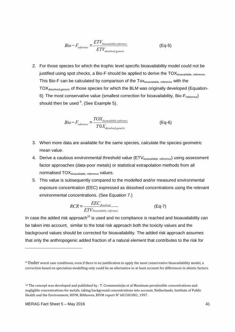
MERAG Fact Sheet 5 – May 2016
41
Bio-Freference =ETVbioavailable,reference
ETVdissolved,generic
(Eq-5)
2. For those species for which the trophic level specific bioavailability model could not be
justified using spot checks, a Bio-F should be applied to derive the TOXbioavailable, reference.
This Bio-F can be calculated by comparison of the Toxbioavailable, reference with the
TOXdissolved,generic of those species for which the BLM was originally developed (Equation-
6). The most conservative value (smallest correction for bioavailability, Bio-Freference)
should then be used 9. (See Example 5).
Bio-Freference =TOXbioavailable,reference
T0Xdissolved,generic
(Eq-6)
3. When more data are available for the same species, calculate the species geometric
mean value.
4. Derive a cautious environmental threshold value (ETVbioavailable, reference) using assessment
factor approaches (data-poor metals) or statistical extrapolation methods from all
normalised TOXbioavailable, reference values.
5. This value is subsequently compared to the modelled and/or measured environmental
exposure concentration (EEC) expressed as dissolved concentrations using the relevant
environmental concentrations. (See Equation 7.)
RCR =EECdissolved
ETVbioavailable, reference (Eq-7)
In case the added risk approach10 is used and no compliance is reached and bioavailability can
be taken into account, similar to the total risk approach both the toxicity values and the
background values should be corrected for bioavailability. The added risk approach assumes
that only the anthropogenic added fraction of a natural element that contributes to the risk for
9 Under worst case conditions, even if there is no justification to apply the most conservative bioavailability model, a
correction based on speciation modelling only could be an alternative to at least account for differences in abiotic factors.
10 The concept was developed and published by : T. Crommentuijn et al Maximum permissible concentrations and
negligible concentrations for metals, taking background concentrations into account, Netherlands, Institute of Public
Health and the Environment, RIVM, Bilthoven, RIVM report N° 601501001, 1997.

MERAG Fact Sheet 5 – May 2016
42
the environment should be regulated/controlled. Although this approach acknowledges that
negative effects from the bioavailable fraction of the background concentration on some
organisms in the ecosystem may occur or that organisms may even have become
acclimated/adapted to it, from an environmental policy point of view, such effects may be
ignored and may even be regarded as desirable, because these effects may in theory lead to an
increase in ecosystem differentiation or biodiversity (Crommentuijn et al 1997). Potential
environmental risks (RCR) are characterised based on the following quotient (Equation 8):
RCR =EECadd,bioavailable
ETVadd, bioavailable
(Eq-8)
Where EECadd,bioavailable = (EECtotal – Cbsite/region)bioavailable and ETVadd, bioavailable = (ETVtotal – Cb culture
medium) bioavailable
Example 5a: Derivation conservative BIO-F value (RWC-cross-species extrapolation)
As indicated in the guidance, the most conservative Bio-F value should be used in order to correct for
bioavailability if there is no justification for full cross-species extrapolation. This was initially the case for
zinc where three chronic BLMs are available for algae, fish and daphnids but no spot checks. Hence at
the time for each, the chronic NOEC values for algae, daphnids and fish were predicted at a site or a
region X, using the BLMs under the site-specific conditions or water chemistry of that site or region. This
will result in NOECx values for that site or region. The chronic NOECx values were then to be compared
with a reference NOEC value (NOECref). This NOECref value is calculated using the BLMs under
reference water chemistry conditions.
Species NOECref
O. mykiss 184
D. magna 86
P. subcapitata 21
Table 5.1: Summary of reference NOEC values (NOECref) for the three aquatic species for which BLMs
have been developed under reference water chemistry conditions11
.
11 The reference water chemistry conditions (ref) are taken from the GEMS-B database (see Table 4.11 in
Heijerick et al 2003). The water chemistry conditions are selected as follows. For all organisms: 10th

MERAG Fact Sheet 5 – May 2016
43
This NOECref is a reasonable worst-case situation that mimics the situation where bioavailability of zinc is
very high and thus can be regarded as a reference value for the bioavailability at the site or region X. The
NOEC at the site or region X (NOECX) is then regarded as a surrogate for the actual bioavailable
concentration of zinc at that site or region X, and is calculated with the BLM-models for the algae,
daphnid and fish. Furthermore, the BLM models provide sufficiently conservative outcomes that are in
good accordance with the generic PNEC. Moreover, the BLM estimates generally overestimate toxicity,
ie, the predicted NOEC values are lower than the experimental values, which provides further support
that the BLMs result in sufficiently conservative outcomes. Therefore, the BLMs are regarded as being
sufficiently validated and sufficiently conservative, thus protective of aquatic organisms.
The bioavailability factors (BioF) are then derived for each of the three (3) BLM species as follows:
BioFwater,X =NOECref
NOECx
The highest value of the three Bio-Fwater,X values for the three species is selected to ensure that a
conservative approach and bioavailability factor (Bio-F) is taken, ie, the smallest correction for
bioavailability.
For zinc, spot checks have been conducted and full cross-species normalisation is allowed. In that case,
if the bioavailability correction needs to be applied on the exposure side, the Bio-F is calculated on the
ETV level (see example 5b).
BioFwater,X =ETVref
ETVx
Example 5b: Bio-F using a full cross-species extrapolation.
In this case study, 29 stations at several Slovakian freshwater bodies were sampled to measure dissolved
Zn concentrations. Ca, pH and DOC were documented by the Slovak Hydrometeorological Institute
(http://www.shmu.sk). As EU reference EQS for Zn, the value of 10.9 µg/L derived by the UK authorities
for the EU commission in 2010 has been used. This value is an EQS “added” (ie, to be added to the
natural background). According to the FOREGS database, the natural background for Zn is 2.7 µg/L. As a
first screen, Zn dissolved concentrations were compared to the EU reference EQS. Only 6 stations did
not exceed this threshold. Therefore 23 sampling stations were potentially at risk.
percentile of DOC. For D. magna and O. mykiss: 10th percentile of inorganic parameters (including pH and
hardness). For P. subcapitata: 90th percentile of inorganic parameters (including pH and hardness).
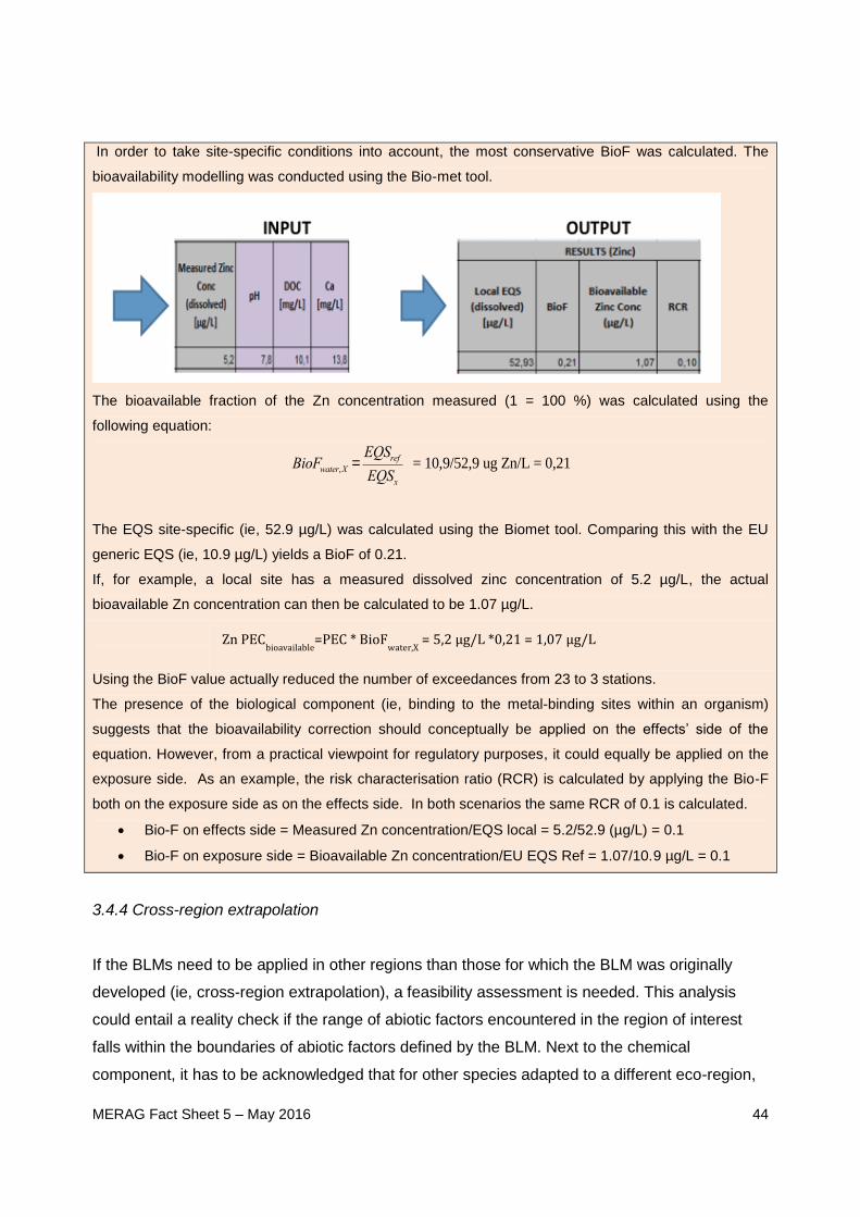
MERAG Fact Sheet 5 – May 2016
44
In order to take site-specific conditions into account, the most conservative BioF was calculated. The
bioavailability modelling was conducted using the Bio-met tool.
The bioavailable fraction of the Zn concentration measured (1 = 100 %) was calculated using the
following equation:
BioFwater,X =EQSref
EQSx = 10,9/52,9 ug Zn/L = 0,21
The EQS site-specific (ie, 52.9 µg/L) was calculated using the Biomet tool. Comparing this with the EU
generic EQS (ie, 10.9 µg/L) yields a BioF of 0.21.
If, for example, a local site has a measured dissolved zinc concentration of 5.2 µg/L, the actual
bioavailable Zn concentration can then be calculated to be 1.07 µg/L.
Using the BioF value actually reduced the number of exceedances from 23 to 3 stations.
The presence of the biological component (ie, binding to the metal-binding sites within an organism)
suggests that the bioavailability correction should conceptually be applied on the effects‟ side of the
equation. However, from a practical viewpoint for regulatory purposes, it could equally be applied on the
exposure side. As an example, the risk characterisation ratio (RCR) is calculated by applying the Bio-F
both on the exposure side as on the effects side. In both scenarios the same RCR of 0.1 is calculated.
Bio-F on effects side = Measured Zn concentration/EQS local = 5.2/52.9 (µg/L) = 0.1
Bio-F on exposure side = Bioavailable Zn concentration/EU EQS Ref = 1.07/10.9 µg/L = 0.1
3.4.4 Cross-region extrapolation
If the BLMs need to be applied in other regions than those for which the BLM was originally
developed (ie, cross-region extrapolation), a feasibility assessment is needed. This analysis
could entail a reality check if the range of abiotic factors encountered in the region of interest
falls within the boundaries of abiotic factors defined by the BLM. Next to the chemical
component, it has to be acknowledged that for other species adapted to a different eco-region,
Zn PECbioavailable
=PEC * BioFwater,X
= 5,2 μg/L *0,21 = 1,07 μg/L

MERAG Fact Sheet 5 – May 2016
45
a comparison in sensitivities between the different species in that region and those used in the
BLM models could be warranted. If deemed appropriate, the SSD could be reconstituted on the
relevance of the culture conditions for the region under consideration or could include species
relevant for the region (temperate species vs tropical species). Recently, alongside the
experience in European freshwater bodies (EU Regional Risk Assessments (RARs) for Ni, Cu,
Zn; van Sprang et al 2009), experience has been gained to assess freshwater quality using
BLMs in different regions worldwide. For example, in Japan (Hayashi 2013), South and Central
America (Natale and Leis 2008; Villavicencio et al 2011; Casares et al 2012), and in North
America (eg Khan et al 2012), several ongoing programmes are successfully demonstrating the
applicability of the Biotic Ligand Model to sensitive fish and invertebrate species in important
tropical/subtropical freshwater ecosystems such as the Everglades (USA), Amazon Basin
(Brazil) and the Mekong/Lancang Basin (Southeast Asia). A larger programme is calibrating the
copper BLM to another diverse tropical/subtropical river system – the Mekong/Lancang,
stretching from mountainous Yunnan Province in China to its delta in southern Vietnam. Here,
BLM application studies on sensitive fish and invertebrates are being conducted (Wu et al 2014;
Wang et al 2014a, 2014b; Chen et al 2014). Initial results again demonstrate that the copper
BLM, developed from temperate species and water types, can successfully be calibrated to
tropical species and environmental conditions. Most studies are based on acute toxicity testing
over a range of physical/chemical conditions. Studies are underway on chronic toxicities.
3.5 Importance of dietary route of toxicity of metals
Information on the relevance of the dietary route for metal toxicity to pelagic organisms has
received increasing attention that provide a number of studies utilising systematic comparisons
of toxicity of metals to an organism via water-only, diet-only, and combined water + diet
exposures. The influence of dietary exposure on steady state tissue concentration has been
well-established (Luoma and Rainbow 2005). In the past, studies investigating if dietary metal
exposure could cause toxicity to aquatic invertebrates provided little insight (Meyer et al 2005;
De Schamphelaere et al 2004, 2007). Recently DeForest and Meyer (2014) reviewed the state
of science about dietborne-metal toxicity to aquatic biota, with a focus on 13 metals: Ag, Al, As,
B, Cd, Co, Cu, Cr, Mo, Ni, Pb, V, and Zn. Of those metals, Ag, As, Cd, Cu, Ni, and Zn have
been demonstrated to cause dietborne toxicity to aquatic organisms in laboratory exposures at
potentially environmentally relevant concentrations. That is, waterborne concentrations at or
near existing waterborne criteria and guidelines (eg, AWQC, EQS values, PNEC values)
sometimes result in dietborne concentrations that contribute to added toxicity to the most

MERAG Fact Sheet 5 – May 2016
46
sensitive species (usually filter-feeding herbivores like freshwater daphnids and saltwater
copepods) beyond the toxicity caused by waterborne exposure alone. However, up to now
dietborne exposures have not yet shown adverse ecological impacts, ie, increased tissue
concentrations have not been linked to adverse population/community effects. Although dietary
exposure is not intrinsically incorporated in the BLM, the organisms in chronic toxicity tests are
fed with algae that will absorb metals during the experiment, and hence the dietary component
is covered to some extent and as such reflected in the derived-BLM parameters (stability
constants).
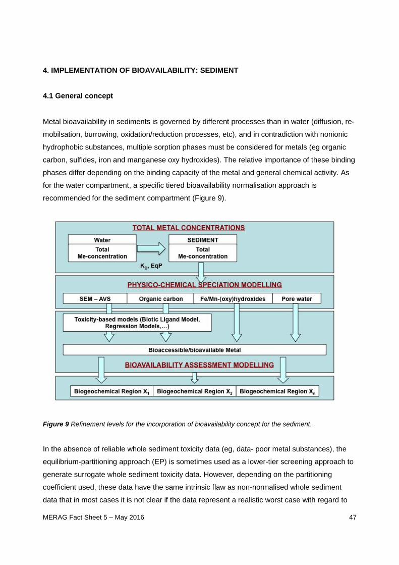
MERAG Fact Sheet 5 – May 2016
47
4. IMPLEMENTATION OF BIOAVAILABILITY: SEDIMENT
4.1 General concept
Metal bioavailability in sediments is governed by different processes than in water (diffusion, re-
mobilsation, burrowing, oxidation/reduction processes, etc), and in contradiction with nonionic
hydrophobic substances, multiple sorption phases must be considered for metals (eg organic
carbon, sulfides, iron and manganese oxy hydroxides). The relative importance of these binding
phases differ depending on the binding capacity of the metal and general chemical activity. As
for the water compartment, a specific tiered bioavailability normalisation approach is
recommended for the sediment compartment (Figure 9).
Figure 9 Refinement levels for the incorporation of bioavailability concept for the sediment.
In the absence of reliable whole sediment toxicity data (eg, data- poor metal substances), the
equilibrium-partitioning approach (EP) is sometimes used as a lower-tier screening approach to
generate surrogate whole sediment toxicity data. However, depending on the partitioning
coefficient used, these data have the same intrinsic flaw as non-normalised whole sediment
data that in most cases it is not clear if the data represent a realistic worst case with regard to

MERAG Fact Sheet 5 – May 2016
48
bioavailability of the metal under scrutiny. As a result, any EQS derived from sediment toxicity
data solely expressed on a total metal concentration (dry or wet weight basis) has the potential
to under or overestimate the risk. Therefore, procedures based on total concentrations have to
be improved by taking into account those factors that governs bioavailability in sediments.
Physico-chemical speciation and (bio)availability is taken into account, eg by estimating the
amount of metal bound to organic carbon, Fe/Mn (oxy)hydroxides, and/or sulfides. The latter,
Acid Volatile Sulfides (AVS), is a key partitioning phase controlling cationic metal activity and
metal-induced toxicity in the sediment interstitial water system (also known as pore water) is
(US EPA 2005). In addition, partitioning to Fe-Mn (oxy)hydroxides, speciation calculations
(reduced forms under anoxic conditions – that is lacking oxygen) and interactions with dissolved
and particulate organic carbon play a role. In case specific bioavailability models are available,
attempts can be made to normalise the whole effect database towards the specific
bioavailability conditions prevailing at a site.
4.2 Equilibrium partitioning approach (EqP)
The possible uncertainties introduced by the use of the EqP approach for metals need to be
carefully weighed against the potential benefits of using the data (eg weight of evidence (WoF),
screening method for data-poor metal substances). The EqP approach was originally developed
for non-ionic organic compounds where it was shown that in absence of real sediment toxicity
data the method could be used to predict sediment toxicity data from water only exposures
taking into account the partitioning behavior of the compound and assuming that the pore water
is the primary route of exposure. Because sediment toxicity data for some metals are also still
lacking, this EP approach has already been applied to metals. However, validation studies of
this concept to metals are scarce. Van Beelen et al (2003) studied the validity of the EP method
for both organic compounds as metals to predict toxicity values for the soil compartment. The
results showed that the EqP method can give significant over-or underestimations, due to
inaccurate and widely variable partitioning coefficients or differences in species sensitivities
(aquatic versus terrestrial species). The HC5-50 values derived using the EP method were in 5%
of the cases more than 20 times higher than the corresponding HC5-50 values that were derived
directly from soil toxicity tests (Van Beelen et al 2003). The Dutch Health Council stated that the
EqP method was only suited for organic, apolar and not for very hydrophobic substances and
not for metals (Gezondheidsraad 1995) because the variation in different partition coefficients
for a single metal is large, introducing quite some uncertainty to the system. Because of this
wide variability, the use of Kp values for the purpose of equilibrium partitioning was not

MERAG Fact Sheet 5 – May 2016
49
recommended for the derivation of ecotoxicological risk limits for metals in sediment
(Verbruggen et al 2001). It is also very important to note that pore water geochemistry will vary
substantially from that of the overlying water, eg, higher DOC, different pH, higher hardness etc.
Overall, the results of whole sediments tests should be preferred because both the dietary and
aqueous routes of exposure pathways are covered in these experimental designs. However, if
the EqP approach is used in a screening approach, care should be taken to use relevant Kd
values that reflect the bioavailability conditions occurring at the site. Because the EP approach
is mainly focused on estimating exposure via pore water, it could be more worthwhile to look at
pore water concentrations using peepers to collect these interstitial waters.
4.3 Physico-chemical speciation modeling
Similar to the water compartment, procedures based on total concentrations have to be
improved by taking into account those factors that drive bioavailability of metals in sediments.
Sulfides are a key partitioning phase controlling cationic metal activity (Hg, Ag, Cu, Pb, Cd, Zn,
Ni) and metal-induced toxicity in the sediment interstitial water system (US EPA 2005).
Additionally, organic carbon plays an important role in copper bioavailability and binding to
Fe/Mn (oxy)hydroxides has been proven to be important for nickel (Costello et al 2011). Even
change in redox potential, and hence speciation, may govern metal toxicity as demonstrated
with chromium where at a negative redox potential chromium is present in its less toxic trivalent
form (Berry et al 2004).
4.3.1 Sulfides binding
Acid Volatile Sulfides (AVS) has been demonstrated to be one of the most important factors
controlling metal toxicity in anoxic and suboxic sediments (Di Toro et al 1990, 1992; US EPA
2005). AVS is, however, in the first place an operationally defined parameter indicating those
sulfides that are readily extracted by the cold extraction of sediment in approximately 1 M HCl
acid. Another term that is used in conjunction with AVS is SEM. SEM (Simultaneously Extracted
Metal) can be defined as the metal, which is simultaneously extracted under the same
conditions under which the AVS content is determined. If multiple metals are present, it is
necessary to use the term total SEM (Σ SEM). The equivalent extraction of sulfide (AVS) and
metal, however, does not necessarily mean that the metal is bound by sulfide alone. SEM refers
to the metal associated with the sulfides and any other metal-bearing phase that is extracted in
the cold HCl extraction used for AVS analysis (Allen et al 1993). For example, metals adsorbed
to iron oxides and particulate organic carbon will also be extracted.

MERAG Fact Sheet 5 – May 2016
50
The fraction of metals that may bind to sulfides in the sediment can be estimated using the
SEM-AVS concept. In case the molar concentration of sulfides exceeds the molar concentration
of metals, then the metals will precipitate and pore water metal concentrations are expected to
be low. If the molar concentration of AVS is lower than the amount of metals present in the
sediment, the SEM-AVS difference gives the amount of SEMMe that is not bound (excess
SEMMe) and consequently metals potentially bioavailable via the pore water. In the pore water,
other important ligands such as organic carbon and Fe/Mn oxides in the sediment or pH, DOC
and hardness conditions in the pore water may further reduce bioavailability. The nomenclature
of excess SEMMe has to be interpreted as “bioavailable” for purposes of estimating the extent to
which metal/metal compounds in sediments may cause toxicity (Equation-9).
MeAVSΔ MelebioavailabMe SEM,SEM (Eq-9)
In applying the SEM-AVS model for a specific metal, it has to be considered that metals
are acting in a competitive manner when binding to AVS. This depends on the solubility
limit of the metal-sulfide complex. The lower the solubility product, the more stable the
MeS complex. Ranked from the lowest to the highest solubility product, the following
sequence is observed: SEMHg, SEMAg, SEMCu, SEMPb, SEMCd, SEMZn and SEMNi,
indicating mercury has the highest affinity for AVS, followed by silver, copper, lead,
cadmium, zinc etc until the AVS is exhausted. The remaining SEM is that amount
present in excess of the AVS.
The SEM-AVS concept has proven to be successful to predict the lack of toxicity in
spiked and field sediments. The concept is limited, however, in terms of predicting
toxicity. Indeed the SEM-AVS concepts indicate how much metals are bound to sulfides
and hence not bioavailable. But even if some metals are not bound to sulfides, it does
not mean that we will see toxicity. That depends on the concentration of freely available
metal and also on the real bioavailability of the metals in the pore water. That is why
SEM-AVS < 0 is a good predictor of absence of toxicity but if SEM-AVS> 0, that is not a
good predictor of the start of toxicity. Toxicity will depend on the magnitude of metal
exceedance of the sulfide and whether the bioavailable threshold is reached and does
not always predict the absence of bioaccumulation (De Jong et al 2009/2010; Lee et al
2000). (See section 4.6).
The SEM-AVS concept works mainly for metals occurring as cations (eg, Cu2+, Zn2+,
Pb2+, …). Anionic forms such a oxyanions (eg, MoO42-, Sb(OH)6
-, …) are not covered.

MERAG Fact Sheet 5 – May 2016
51
Although metal sulfides can account for much of the non-toxic metal, it should be
recognized that excess SEM can be bound to organic carbon (OC) and that sediment
iron and manganese oxides may further reduce the fraction of bioavailable metal. The
current SEM-AVS approach may therefore overestimate bioavailable metal and its
toxicity towards sediment organisms in oxic surface layers with sufficient Fe and Mn to
bind other metals (Costello et al 2011).
4.3.2 Binding to other sediment phases (organic carbon, Fe/Mn-(oxy)hydroxides
Organic carbon has been identified as one of the major drivers for copper toxicity in sediments,
but also other metals show a high affinity to bind with organic carbon sources. The affinity of
metals to bind with organic carbon has been used by Di Toro et al (2001, 2005) as the premise
to build a model to predict not only the lack, but also the onset, of metal toxicity in spiked and
field- contaminated sediments (Di Toro et al 2001, 2005). In this context, it is assumed that
toxicity occurs if the excess SEM goes beyond the binding capacity of the organic carbon
present in the sediment. Using this information, it was shown that the organic carbon-
normalised excess SEM can be used to predict toxicity (Equation-10):
fOC
AVSSEMocSEMx
, (Eq-10)
Where fOC is the organic carbon fraction in the sediment.
But even in the absence of AVS (ie, aerobic sediment), it is worthwhile exploring if a linear
relationship can be established between the observed toxicity levels of the metal and the
presence of organic carbon. If a relationship can be discerned, the variability introduced by the
presence of toxicity values generated at different organic carbon concentrations can be
captured by normalising each Tox value using the following formula:
TOXOC, normalized =TOXtotal
fOC (Eq-11)
TOXtotal (mg Me/kgdw); dw = dry weight
fOC = fraction organic carbon
TOXOC, normalised (mg/g OC)
MERAG Fact Sheet 5 – May 2016
52
Fe and Mn oxides have been identified by different authors as important factors controlling
bioavailability of certain metals such as nickel (Costello et al 2011). These phases are
particularly important because they have a large sorption capacity. Furthermore, they appear as
coatings on the particles and occlude the other mineral components. As soon as reliable
quantification models become available or equations have been established, the parameters
could also be accounted for in the bioavailability correction in sediment.
4.3.3 Use of metal concentrations measured in pore water
When dealing with bioaccessibility/bioavailability in sediments, it is suggested that the best
metric for the moment is the freely dissolved pore water concentration, both for metals and
organic chemicals (ECHA 2013). This is particularly true for selected cationic metals. Of course,
if it can be expected that the dietary route could contribute significantly to the exposure (ie,
conditions in the digestive track differ markedly from those in the sediment, then the
assessment should not only focus on the pore water but should also take sediment ingestion
into account (section 3.6).
New Paragraph here
Dissolved metal pore water concentrations could be measured in pore water collected by
different passive sampling methods (Peijnenburg et al 2014). Despite significant advances in
the development and application of these devices, practical incorporation of these methods in
contaminated sediment management decisions has been limited. Pore water concentrations are
not often analysed in ecotoxicity tests and for many metals accurate pore water measurements
can be difficult because the separation of pore water from sediments often results in
experimental artifacts. To ensure consistency in the approaches to assess the bioavailable
concentration in sediment pore water and overlying water, additional research is recommended
before pore water normalisation can be routinely used.
4.4 Use of toxicity-related bioavailability models
Although the SEM-AVS approach has been proven to be quite accurate by demonstrating the
absence of sediment-associated toxicity for metals, it is less useful in predicting the occurrence
of toxic effects. Mechanistically based bioavailability models (sediment BLMs) or empirically
based regression models predicting the metal toxicity in spiked sediments based on sediment
properties (eg, AVS, TOC, Fe/Mn) are available or may be developed for establishment of
environmental threshold values. The models can be used to normalise the available toxicity
data set to specific bioavailability conditions (see tier 2 section 4.5). Further information on the
MERAG Fact Sheet 5 – May 2016
53
derivation of regression models in general is included in section 5.4.3 dealing with the soil
compartment.
In case no bioavailability model is available for all biological species, care should be taken in the
choice of the bioavailability model to be used in a cross-species extrapolation exercise for the
sediment compartment. As various faunal organisms disturb or alter the sediment structure
differently depending on their specific feeding type, mobility and life cycle (formation micro-
habitats), the bioavailability model developed for another species that resembles a similar life
strategy should be used.
4.5 Tiered implementation in a risk assessment context
The application of physico-chemical speciation modelling and/or the use of toxicity based
bioavailability models are dependent on the knowledge and availability of information on
relevant abiotic factors, and/or established relationships between toxicity and physico-chemistry
of the sediments. Figure 10 represents the tiered approach that can be used to refine the risk
assessment using the knowledge about sediment abiotic factors that drive toxicity (eg AVS or
OC).
MERAG Fact Sheet 5 – May 2016
54
Figure 10 Framework for assessing risks of metals/metal compounds in sediments using the SEM-AVS
approach
The scheme presented in Figure 10 gives the user the ability to perform a robust analysis of the
potential risks depending on the data availability. In the highest tier (Tier 3) actual SEM-AVS
analyses are conducted and a site-specific approach can directly be conducted for those
divalent metals known to bind to AVS. However, in the absence of these data, a more generic
approach using a generic reasonable worst-case environmental threshold value expressed as
total metal concentration could be used (Tier 1) or in case adequate bioavailability models are
available, these could be used to derive the ETV (Tier 2).
In the generic approach (Tier 1) an ETV is chosen to reflect a scenario which maximises
bioavailability and could serve as a conservative benchmark to ensure that results are
protective for the majority of sediments (including those oxic/suboxic sediments). This goal is

MERAG Fact Sheet 5 – May 2016
55
achieved by populating the effect database with toxicity data from tests conducted using spiked
sediments with low AVS/OC/Fe/Mn content that would probably represent high bioavailability
conditions. Test results from sediments with high AVS/OC/Fe/Mn content should be excluded
from the database. If a potential risk is identified in Tier 1 and an adequate regression model
(eg AVS model for Ni, or OC for copper) is available, the ETVRWC can be recalculated toward a
reference situation such as 10th percentile of the regional AVS/OC distribution (Tier 2a) in case
no actual or historical AVS/OC data are available or ETV can be normalised towards the
measured AVS/OC concentrations occurring at the site (Tier 2b). If no AVS-based bioavailability
model is available, the only refinement step is to conduct paired measurements of AVS and
SEM for the particular metal. In that case, the SEM-AVS difference is directly calculated. If
SEM-AVS is < 0, no further action is required. If SEM -AVS is > 0, other lines of evidence can
be explored (eg direct toxicity testing, macroinvertebrate analysis, etc). The different tiers are
further elaborated in the subsequent sections.
TIER 1: comparison modelled/measured data with a reasonable worst-case (RWC) ETV
1) The different generic toxicity values that are used in the sediments effects assessment
are generally generated in sediments with varying physico-chemical characteristics
known to alter metal bioavailability and toxicity (eg, low/high AVS, low/high OC). In order
to derive an ETVrwc, only toxicity data from sediments exhibiting reasonable worst-case
conditions for AVS, OC and Fe/Mn should be included in the calculations. Toxicity
results from sediments with characteristics that mitigate metal toxicity (ie, high AVS/
OC/Fe/Mn content) should be excluded.
2) Calculate the ETVrwc from all toxicity (low AVS, low TOC) values. The EQSrwc is expressed as
total metal, which facilitates the comparison with available sediment monitoring
databases that are also mostly expressed as total metal.
3) Calculate the EEC total,sediment from all individual Ctotal values for a predefined
environmental site (local or regional) taking a high end value (eg, the 90th percentile) of
the concentrations of the metal of concern. As a natural sediment in lowland rivers will
probably contain a certain amount of AVS, it is recommended to correct the EEC total by
subtracting the amount of metal that could potentially bind with the sulfides present
(Note: the specific regional background of metals with a higher affinity is subtracted
first). For example, for nearly oxidized sediments, it can be assumed that the AVS
concentration in the sediment is low, ie an AVS concentration of < 1 µmol/g dry wt. can
be used as default value available to bind with sediments. At this stage, it is also

MERAG Fact Sheet 5 – May 2016
56
assumed that the total metal concentration can be used as a conservative estimate of
SEMMe. EECAVS normalized is then calculated using Equation-12.
EEC AVS normalised = EECtotal - AVSdefault (Eq-12)
EECMe, total expressed as µmol/g.dry wt.
{AVS} = {AVStotal} - {SEMHg}- {SEMAg}. …… (this computation is repeated until the next least
soluble metal sulfides).
4) The risks for a local or regional environment are subsequently calculated from the
comparison between the EECtotal, sediment and the ETVrwc (Equation-13). Both parameters
are expressed as mg total Me/kg dry wt.:
RCR =EECtotalmetal
ETVrwc (Eq-13)
TIER 2: Normalisation using toxicity-based models
1) Link the NOEC/ECX values of the chronic ecotoxicity database (as total metal
concentrations) with the relevant sediment parameters of the sediment (eg AVS, OC) in
which the test was performed.
2) If regression models, taking the form log(ECx) = intercept + slope * log(abioticfactor),
have been developed, the corresponding organisms specific slopes (from the
regression analysis) can be used to normalise the NOEC/ECX values to “reasonable
worst case” sediment properties (eg 10th percentile AVS) or to specific local/regional
conditions (actual or historical AVS concentrations prevailing on the site under
investigation). The normalisation equations for RWC-and site-specific conditions is given
here below (Equation-14 and Equation-15) are:
ECXRWC = ECXtestabioticfactorRWC
abioticfactortest
é
ëê
ù
ûú
slope
(Eq-14)
Where test = scenario with typical local or regional conditions for which the Tox,test is derived,
and RWC = the realistic worst case scenario is used as a reference scenario when correcting
bioavailability with toxicity-related models providing us with a Tox,RWC corresponding to a
maximised bioavailability.

MERAG Fact Sheet 5 – May 2016
57
ECXSite-specific = ECXtestabioticfactorSite-specific
abioticfactortest
é
ëê
ù
ûú
slope
(Eq-15)
Where test = scenario with typical local or regional conditions for which the Tox,test is derived
and site-specific = reflects the local AVS conditions.
3) Derive a ETVrwc or a ETVsite-specific using an SSD or AF approach.
4) The risks for a local or regional environment are subsequently calculated from the
comparison between the EECtotal, sediment and the ETV rwc /site specific (Equation-16):
RCR =EECtotalmetal
ETVrwc / sitespecific
(Eq-16)
In case organic carbon has been identified as the major driver (eg copper), the ETV sediment
can be calculated back to mg/kg dry wt. when a default OC value is assumed for the
area/region under investigation. The latter value can be used as a generic ETV. In the EU, a
standard sediment has a default OC value of 5 %. The risks for the local site can subsequently
be calculated from the comparison between the EECtotal and the RWC ETVnormalised, OC (5%) taking
into account site-specific information on the OC content (Equation-17)
RCR =EEC
ETVnormalized ,OCregion´fOCsite
fOCregion
(Eq-17)
TIER 3: Application of the SEM-AVS concept if actual measured regional/local SEM-AVS
concentrations are available
The SEM-AVS concept can be applied to a specific region or a local site if extensive SEM-AVS
data representative for that region or if site-specific local SEM-AVS measurements are
available. Considering the observed co-variance between AVS and SEMMe, it is recommended
to take only measured-coupled data into account to maintain the ecological relevance of the
analysis (Vangheluwe et al 2003, 2008). Low AVS-high SEM combinations are unlikely to be
found. Knowledge with respect to spatial and seasonal variations of AVS and SEM levels is
required for a proper application of the AVS concept in this context. SEM-AVS data should

MERAG Fact Sheet 5 – May 2016
58
represent the seasonal worst-case scenario (ie lowest AVS levels being measured, spring
season). In addition, as there exist a redox gradient in sediments, AVS levels tend to decrease
with decreasing depth, as the redox potential in surficial sediments can be positive or less
negative than deeper sediments. It is important to focus the analysis on the biologically active
layer of the sediment (0-20 cm). But even over this depth, the AVS profile could differ
dramatically, and in top layers (0-2 cm) a significant lower amount of AVS can be present or can
be even completely absent. Incorporation of measured SEM-AVS data in the risk
characterisation should be performed as outlined here below.
1) From the compiled SEM and AVS data set, the potential bioavailable SEMMe fraction for
each individual sampling point is derived by coupling the AVS and SEMMe data for that
specific station.
EEC AVS normalised = SEMMe, sampling point 1 - AVSsampling point 1 (Eq-18)
2) For the regional scenario, a distribution function of all individual (SEMMe - AVS) values
across the region is elaborated. The EECAVS normalised, regional is calculated as the higher
value (eg 90th percentile) of the measured bioavailable SEMMe.
3) For the local scenario, the EEC AVS normalised, local is taken as such.
4) If this value is < than 0, then 100 % of SEMMe is bound to sulfide and no toxicity (risk) is
expected to occur (Equations 15-16 example local scenario). In case this difference is >
than 0 (meaning not enough AVS is available for binding with the SEMMe), metals are
potentially bioavailable and could, if present in high enough amounts, elicit a toxic
response or present a risk to the sediment compartment.
SEMMe, sampling point 1 - AVSsampling point 1 < 0 (no risk scenario) (Eq-19)
SEMMe, sampling point 1 - AVSsampling point 1 > 0 (potential risk scenario) (Eq-20)
In case SEM-AVS > 0, a further weight of analysis can be conducted (eg direct toxicity testing,
macro-invertebrate analysis etc).

MERAG Fact Sheet 5 – May 2016
59
Example 6: Incorporation of bioavailability in the risk characterisation of Ni metal and chemical
producer (Ni sulphate and Ni carbonate)
As a hypothetical example, a nickel metal and nickel chemical producing plant is located in Finland (site A).
It is assumed that the site reported measured SEM-AVS data. This site, encoded ChP003, has been
selected as an example to demonstrate the way bioavailability refinements can be incorporated in the
overall sediment risk characterisation framework. For Ni, a bioavailability model is available so RWC EQS
value of 109 mg Ni/kg dry wt. can be calculated by normalising the ecotoxicity data to RWC conditions
reflected by the 10th percentile of the AVS concentrations present in European sediments.
TIER 2a: Bioavailability refinement using default AVS concentrations: comparison modelled/measured data
with RWC EQS normalised to a default AVS concentration.
Applying the bioavailability models for the different species for a 10th percentile AVS default concentration
(0.8 µmol/g dry wt Flemish database) yields a RWC PNEC of 109 mg/kg dry wt. With the default RWC AVS
concentration, risks are still identified (Table 6.1.).
Site Clocal
(mg Ni/kg dry
wt)
PECregional
(mg Ni/kg dry
wt)
PECtotal
(mg Ni/kg
dry wt)
EQS normalized
10th
percentile
AVS
RCR
Site A 85.8 61.2 147 109 1.3
Table 6.1: Overview exposure data and risk characterisation-tier 2a
TIER 2b: Bioavailability refinement using default AVS concentrations: comparison modelled/measured data
with RWC PNEC normalised to the AVS concentration likely to occur in the region.
If AVS concentrations are available from earlier AVS measurements in the river sediments or from rivers in
the region with similar characteristics, an assessment can be made of the identified risks that are probable
to occur. It is assumed that for the receiving Finnish river an AVS concentration of 8.0 µmol/g dry wt has
been measured in the past. The RWC PNEC was subsequently normalised towards this AVS
concentration yielding a EQS normalised of 225 mg/kg dry wt (Table 6.2).
Site Clocal (mg
Ni/kg dry wt)
PECregional
(mg Ni/kg dry
wt)
PECtotal
(mg Ni/kg
dry wt)
EQS
normalized
to historical
AVS data
RCR
Site A 85.8 61.2 147 225 0.7
Table 6.2: Overview exposure data and risk characterisation- Tier 2b

MERAG Fact Sheet 5 – May 2016
60
Using the available AVS concentration for the river, it is unlikely that a risk will occur at the site (RCR < 1).
TIER 3: Bioavailability refinement using actual measured SEM-AVS data: site-specific approach to
calculate the actual risks.
If actual SEM and AVS measurements were made upstream and downstream of the plant (Table 6.3), a
site-specific approach can be followed.
Sediment
(µmol/g dry wt))
SEM Cu SEM Pb SEM Cd SEM Zn SEM Ni Σ SEM AVS SEM-AVS
Downstream 0.083 0.044 0.002 0.439 1.118 1.686 6.18 < 0
Upstream 0.268 0.047 0.004 0.456 0.945 1.720 8.2 < 0
Table 6.3: Overview exposure data and risk characterisation- Tier 3
The AVS concentration measured downstream from the plant, ie, 6.2 µmol/g dry wt. is similar to the value
measured in 2007 (ie 8.0 µmol/g dry wt). The SEM-AVS calculation taking into account all metals present at
the site is less than 0, predicting the absence of metal-induced toxicity and hence no local risk.
Example 7: Application of bioavailability models in the EQS derivation for nickel for
freshwater sediments.
For nickel, chronic sediment toxicity tests are available for 10 species of sediment-dwelling
organisms conducted in nickel-spiked sediments representing sediments with low and high
nickel-binding capacity (ie low AVS/low TOC and high AVS/high TOC). In addition, chronic
toxicity tests were conducted with several additional nickel-spiked sediments with a wide range of
AVS and TOC concentrations in order to characterise relationships for 7 test species between
nickel toxicity and sediment characteristics (ie bioavailability regression models) (Table 7.1)
(Vangheluwe and Nguyen 2015; Besser et al 2013).
Table 7.1: Overview slope and intercepts of the different bioavailability models.
Species Life strategy Intercept
(S.E)
Slope
(S.E.)
H. azteca Swimmer, sprawler, surface deposit feeder 2.65
(0.11)
0.492
(0.11)
S. corneum Burrower, surface deposit feeder 2.73
(0.01)
0.478
(0.011)

MERAG Fact Sheet 5 – May 2016
61
G. pseudolimnaeus Swimmer, sprawler, surface deposit feeder 2.8
(0.13)
0.358
(0.13)
Hexagenia sp. Burrower, surface and subsurface feeder 2.35
(0.06)
0.175
(0.07)
C. riparius Burrower, surface and subsurface feeder 2.85
(0.017)
0.180
(0.017)
T. tubifex Burrower, subsurface feeder 3.05
(0.006)
0.125
(0.006)
The normalisation procedure used the following equation:
ECXRWC = ECXtestabioticfactorRWC
abioticfactortest
é
ëê
ù
ûú
slope
Using the bioavailability models, data were normalised towards the realistic worst case (RWC)
physico-chemical conditions prevailing in EU sediments (ie 0.8 µmol AVS/g dry wt). An overview
of the normalised species mean L(E)C10 value for the most sensitive endpoint is provided in Table
7.2.
Table 7.2: Overview nickel sediment ecotoxicity database.
Taxonomic
group
Species Most
sensitive
endpoint
Normalised species
mean
(NOEC/L(E)C10
value (mg Ni/kg dry
wt)
Crustaceans Hyalella azteca
Gammarus pseudolimneaus
Biomas
Biomass
203.5
348.4
Insects Ephoron virgo
Hexagenia sp.
Chironomus riparius
Chironomus dilutus
Biomass
Biomass
Development
141.1
188.7
673.5
> 762
Oligochaetes Lumbriculus variegatus
Tubifex tubifex
Abundance
Biomass
529.8
1000.3
Molluscs Sphaerium corneum
Lampsilis siliquoidea
Biomass 322.1
> 762
Subsequently, a log-normal distribution was fitted through the ranked species mean toxicity data.
From this SSD, the median HC5 was calculated using the ETX model. The SSD and the median
HC5 value for the normalised ecotoxicity data towards the RWC AVS conditions prevailing in the
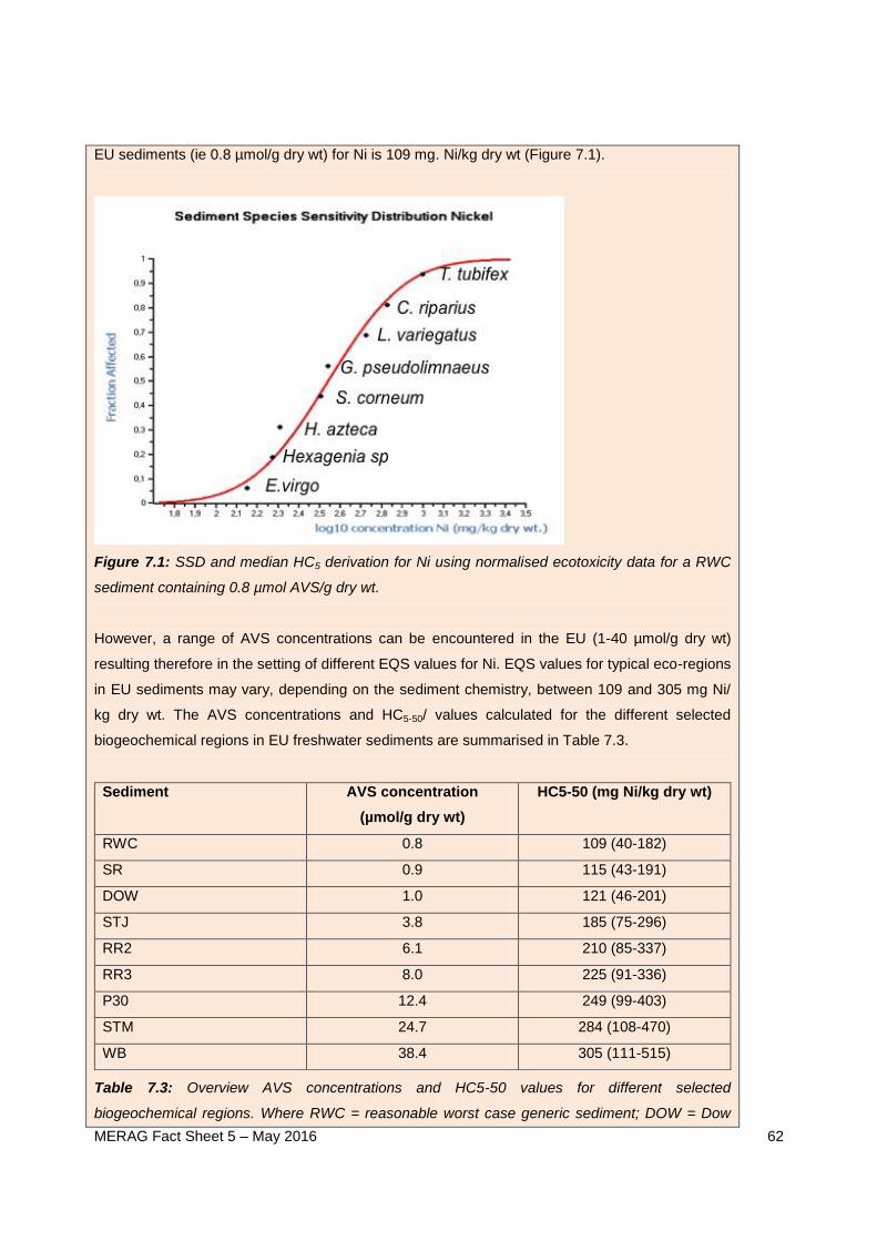
MERAG Fact Sheet 5 – May 2016
62
EU sediments (ie 0.8 µmol/g dry wt) for Ni is 109 mg. Ni/kg dry wt (Figure 7.1).
Figure 7.1: SSD and median HC5 derivation for Ni using normalised ecotoxicity data for a RWC
sediment containing 0.8 µmol AVS/g dry wt.
However, a range of AVS concentrations can be encountered in the EU (1-40 µmol/g dry wt)
resulting therefore in the setting of different EQS values for Ni. EQS values for typical eco-regions
in EU sediments may vary, depending on the sediment chemistry, between 109 and 305 mg Ni/
kg dry wt. The AVS concentrations and HC5-50/ values calculated for the different selected
biogeochemical regions in EU freshwater sediments are summarised in Table 7.3.
Sediment AVS concentration
(µmol/g dry wt)
HC5-50 (mg Ni/kg dry wt)
RWC 0.8 109 (40-182)
SR 0.9 115 (43-191)
DOW 1.0 121 (46-201)
STJ 3.8 185 (75-296)
RR2 6.1 210 (85-337)
RR3 8.0 225 (91-336)
P30 12.4 249 (99-403)
STM 24.7 284 (108-470)
WB 38.4 305 (111-515)
Table 7.3: Overview AVS concentrations and HC5-50 values for different selected
biogeochemical regions. Where RWC = reasonable worst case generic sediment; DOW = Dow

MERAG Fact Sheet 5 – May 2016
63
Creek; P30 = US Geological Survey Pond 30; RR2 = Raisin River (site 2); RR3 = Raisin River
(site 3); STJ = St. Joseph River; STM = south tributary Mill Creek; SR = Spring River; WB = West
Bearskin Lake.
4.6 Relative importance of dietary route for metals in sediments
In assessing risks for the sediment compartment, the dietary route could be of a relative higher
importance than the aquatic compartment. Whole sediment toxicity tests are typically conducted
using an array of test species with different life strategies. Several of these organisms are
dependent on the ingestion and assimilation of sediment particles to survive. If those sediments
have been contaminated with the metal of concern, the dietary route is intrinsically included in
the assessment. For those species getting additional uncontaminated food, the dietary
exposure could be underestimated. Further scientific research is, however, needed to assess
the relative importance of the dietary route and its consequences for risk assessment purposes.
In relation to this, it is essential to evaluate if the SEM-AVS model still holds for predicting that
no toxicity should occur when excess AVS is present. Studies examining the bioaccumulation
of metals in anaerobic sediments showed, in general, that in most of the cases, metal
accumulation is reduced when SEM-AVS < 0 (Ankley et al 1996). However, in some cases,
bioaccumulation was best correlated with total metal content in the sediment irrespective of the
AVS content (Lee at al 2000; De Jonge et al 2009, 2010). It has been found that the dietary
route seems to play an important role in explaining these observations. It should, however, be
kept in mind that bioaccumulation does not represent a toxicological effect and an unambiguous
connection between observed levels of accumulation and effects is not frequently observed. For
species with no important detoxification mechanisms (eg Hyalella azteca), however, a
relationship between internal body concentration and effects is well documented (Environment
Canada 2011). But, in general, when detoxification systems are in place, toxicity does not
depend on total accumulated metal concentration but is related to a threshold concentration of
internal metabolically available metal (Rainbow 2007). Toxicity ensues when the rate of metal
uptake from all sources exceeds the combined rates of detoxification and excretion of the metal
concerned. Subsequently, the biological significance of accumulated metal concentrations
under SEM-AVS conditions < 0 will depend on the way organisms cope with the increased
metal exposure. Metals extracted in the gut from the ingested metal sulfides are detoxified and
stored in granules, while at an overload of the AVS system, metals can be found in a more
easily accessible pool (De Jonge et al 2011). Overall, the recent results support the tenet that

MERAG Fact Sheet 5 – May 2016
64
AVS controls metal toxicity via the pore water in particular with relation to chronic effects and
can therefore still be used in a risk assessment framework.
5. IMPLEMENTATION OF BIOAVAILABILITY: SOIL
5.1 Introduction
The total (or aqua regia soluble) metal concentration in soil is often a poor predictor of metal
toxicity to terrestrial organisms. The bioavailability and toxicity of metals or metalloids in soils is
influenced by a number of abiotic factors such as:
i) Variation in soil properties (eg pH, clay content, organic carbon content, (e)CEC)
among soils (Oorts et al 2006a; Song et al 2006; Criel et al 2008; Li et al 2010a,
2010b and 2013);
ii) Time since contamination (ageing processes, Lock et al 2006a; Oorts et al
2006b; Wendling et al 2009);
iii) Form of metal added to the soil (Degryse et al 2004; Ma et al 2013).
Soil properties, such as pH, organic carbon content and texture, determine the amount and
type of metal species available for uptake by plants, invertebrates, and soil microorganisms,
and the resulting toxic response or bioaccumulation of metal. Correction for the variation in soil
properties among soils and hence normalisation to specific characteristics of a soil of interest
requires an understanding of the relationship between soil physico-chemistry and metal toxicity
on microbial function, plants and invertebrates. In order to perform such normalisation,
speciation or bioavailability models must be available, allowing prediction of soil-specific metal
toxicity.
Another aspect that needs to be taken into consideration for soils is that toxicity tests are
typically based on soils that are freshly contaminated with soluble metal salts and results
overestimate toxicity effects in historically contaminated soils at the same total metal level. The
ecological relevance of toxicity tests after freshly spiking is questionable because metal spiking
causes a sudden disturbance that is unrepresentative of a field where metals are added
gradually and could equilibrate for several years.

MERAG Fact Sheet 5 – May 2016
65
In addition to the immediate, short-term effects of soil characteristics on metal bioavailability, it
has also been shown that long-term equilibration (ageing) of metals in soil is a critical factor in
determining bioavailability for most metals. (Italics for emphasis on important point) Long-term
changes in metal bioavailability are due to phenomena such as inclusion of natural elements
into the crystal lattices of soil minerals, the formation of insoluble precipitates, diffusion of
metals into micro pores, etc. Spiking soils with soluble metal salts not only increases the metal
content of a soil, but also increases the ionic strength of the soil solution and decreases the soil
pH by the replacement of protons from the exchange complex with the metal cations. These
changes in pH and ionic strength can also affect the biological response either directly or
indirectly through their effect on metal bioavailability. The natural leaching of the excess cations
and anions avoids these artifacts in field conditions. Both ageing and leaching processes
significantly influence the bioavailable fraction of metals, thereby changing the soil toxicity
profile over longer periods of time.
Most toxicity data for metals are based on tests with soluble metal salts, ensuring maximal
solubility and bioavailability. However, contaminations are often caused by other, less soluble
sources, eg oxides or metallic forms. The form of the metal added to a soil can have a major
impact on its behaviour, bioavailability and toxicity. For example, the solubility and toxicity of the
poorly soluble antimony trioxide in soil increases with time, and soil solution concentrations at
equivalent total Sb concentrations only converge after 5 years with those of the more soluble
SbCl3 (Oorts et al 2008). Although less soluble metal sources in soil may slowly transform into
more soluble forms, thermodynamic equilibrium may only be reached in the long term (years or
decades). At present, there is, however, no generally accepted approach for
implementing considerations on the form and transformation rates of a metal into a risk
assessment of metals in soil.
Although it is generally accepted that the total metal concentration in soil is a poor predictor for
toxicity to the environment, there is not yet a generally accepted method for measurement of the
bioavailable fraction of metals in soil (Menzies et al 2007; Zhao et al 2006). As for the water
compartment, the free metal ion in the pore water is considered to be the bioavailable metal
species. However, expressing metal toxicity in soil based on total soil solution metal
concentration or free metal ion activity generally increases variability in toxicity thresholds
among soils and hence does not explain differences in bioavailability. Several soil extraction
techniques have been used in order to predict metal bioavailability and toxicity in soils (eg pore
water, 0.01M CaCl2, 1 M NH3NO3, 0.43 M HNO3, Diffusive Gradients in Thin-films (DGT),

MERAG Fact Sheet 5 – May 2016
66
cyclodextrin (HPCD), extraction, simulated earthworm gut (SEG) etc). However, no standard
method applicable to most metals and soil types has been identified. If used for regulatory
purposes, this should be done in a cautious way because in their current stage of development,
extraction techniques are generally not validated with metal toxicity data to soil organisms. Most
extractions and tests for bioavailability are indeed calibrated on uptake of metals by plants and
invertebrates and not by their toxic effects to these organisms. Using bioaccumulation to
calibrate soil extractions does not ensure that they predict toxicity, eg because translocation of
metals from plant root to shoot is restricted.
Figure 11: Five different expressions of Cu toxicity (EC50) to tomato seedling shoot yield in 17 freshly
amended soils. Where the coefficients of variance is the standard deviation divided by mean of
untransformed EC50 values. Where DGT = diffusive gradients in thin film technique; eCEC = effective
cation exchange capacity, ie CEC at prevailing soil pH. Data adapted from Zhao et al 2006 and Smolders
et al 2009.
5.2 General concept
Data for (pseudo-) total metal concentrations, based on concentrated acid digestions, are most
commonly available and used for risk assessment purposes. Toxicity data for soil organisms are
preferentially expressed as total metal concentrations. As for water and sediment, a tiered
approach is recommended for refinement of the effects assessment of metals in soil (Figure
12).
0.0001 0.001 0.01 0.1 1.0 10.0 100.0 Cu concentration scale (log scaled)
Cu2+ activity (µM)
Total soil Cu (g Cu/kg)
Soil solution Cu (mg Cu/L)
DGT Cu (mg Cu/L)
Total Cu as percent of eCEC(%)
variation coefficient (%)
70%
117%
279 %
43%
44%

MERAG Fact Sheet 5 – May 2016
67
Figure 12: Refinement levels for the incorporation of bioavailability concept for the soil compartment.
In cases where no reliable toxicity data are available for the terrestrial environment, the
equilibrium partitioning approach (EqP) is sometimes used as a lower tier screening approach
to generate an EQS for soil based on toxicity data for the aquatic compartment and a soil:water
distribution coefficient (Kd). The equilibrium partitioning approach is based on the assumption
that soil toxicity expressed in terms of the freely dissolved metal concentration in the pore water
(interstitial water) is the same as aquatic toxicity. It should be emphasised that substitution of
terrestrial toxicity data by aquatic toxicity data should be used with caution. This is because the
effects on aquatic species can only be considered as effects on soil organisms that are exposed
exclusively to the soil pore water and may hence not be appropriate for organisms also exposed
to soil particles and food via the dietary pathway. Furthermore, studies have shown that the
equilibrium-partitioning method can give significant over- or underestimations, due to inaccurate
partitioning coefficients or differences in species sensitivities between aquatic and terrestrial
species (Van Beelen et al 2003). If the EqP approach is used in the screening, then care should
be taken to use relevant Kd values that reflect the bioavailability conditions occurring at the site.
Overall, the results of toxicity tests in whole soil should be preferred because both the dietary
and aqueous exposure pathways are covered in these experimental designs. As reported
above, natural soils used in ecotoxicological tests differ in physico-chemical characteristics,
TOTAL METAL LEVELS
pH, OC,… (speciation model)
“Free ionic” Me-fraction
Biogeochemical Regions X1, X2, Xn,…
Pore water Me-fraction
Application of Lab-Field Factor
Normalized toxicity threshold
BIOAVAILABILITY ASSESSMENT MODELLING
KD
PHYSICO-CHEMICAL SPECIATION MODELLING
Normalization towards soil of interest (based on toxicity-based regression models)
Water
Total Me-concentration
SOIL
Total Me-concentration
KD, EqP
MERAG Fact Sheet 5 – May 2016
68
which may significantly affect the bioavailability of the test compound, and hence the toxicity
observed. Therefore, any EQS derived from toxicity data expressed on a total metal
concentration, without any further information on bioavailability, has still the potential to under-
or overestimate the risk. In the absence of specific information on the bioavailability of a metal,
toxicity has to be tested in a reasonable worst-case scenario, ie, a soil with assumed high
bioavailability of the metal substance tested as estimated based on physico-chemical speciation
modeling and predicted partitioning. This ensures that results are protective for the majority of
soils. Such reasonable worst-case soils have low organic carbon content (eg >0.5 and <2%)
and low clay content (eg >5 and <10%). The pH would be low (eg <5.5) or high (eg >7) for
metals occurring as cations (eg Cu2+, Zn2+, Pb2+, …) or oxyanions (eg MoO42-, Sb(OH)6
-, …),
respectively.
In case specific bioavailability models are available, toxicity data can be normalized towards the
specific bioavailability conditions prevailing at a site. Bioavailability models were developed to
correct for the differences in bioavailability due to varying soil properties or differences between
lab and field conditions. First, a lab-to-field correction factor is used to translate results obtained
from laboratory experiments to field conditions (see section 0). In a second step, a soil-
dependent correction factor is applied in order to normalise the results towards the specific
physico-chemical conditions of the site of interest (see section 0). Both correction factors are
derived from an empirical approach. At present, no models are available to correct for the form
of metal added (eg soluble salt versus poorly soluble metal compounds) and toxicity data for
soluble metal salts are used as a worst-case reference for all metal forms.
5.3 Mechanistic versus empirical terrestrial bioavailability models
During the last decade, a lot of research has been performed on bioavailability and toxicity of
metals in soil. Physico-chemical soil properties (eg pH, organic carbon and clay content, cation
exchange capacity) are often significantly correlated with metal toxicity for plants, invertebrates
and micro-organisms based on (pseudo-) total metal concentrations in soil. Empirical regression
models are derived, covering a wide range of soil types (Smolders et al 2009). Such regression
models can be used to normalise effects data towards specific conditions of a site of interest
and, hence, allow for the derivation of site-specific threshold concentrations, expressed as total
metal concentration. Additionally, comparison of metal toxicity in laboratory and field conditions
yielded toxicity-based empirical correction factors for differences between laboratory and field
conditions were derived for a range of metals.

MERAG Fact Sheet 5 – May 2016
69
Next to these empirical models, some more mechanistic models were developed. These models
are generally based on the biotic ligand model (BLM) concept as used for bioavailability
corrections for the water compartment. Several levels of complexity are considered in this
research (Figure 13). Most research so far has focused on derivation of biotic ligand models for
terrestrial organisms (plants, invertebrates and micro-organisms) grown in nutrient solutions
(Figure 13A; eg Lock et al 2006b; Antunes et al 2007, Mertens et al 2007). These studies show
that the BLM concepts are also valid for terrestrial organisms and hence illustrate that the free
metal ion in solution is the toxic metal fraction and that its bioavailability depends on competition
with other ions (blue arrows in Figure 13).
In a higher level of complexity, the BLM concept was calibrated with results of toxicity studies in
natural soils. The modeling is, however, based on the composition of the soil solution and at
maximum only the critical free metal ion activity in the pore water was predicted from the total
metal concentration in soil based on a speciation program (Figure 13B; eg, Thakali et al 2006a,
2006b; Lofts et al 2013). These terrestrial BLMs have also been calibrated using data from
freshly amended soils in which the concentrations of the competing ions are higher than those
in field-contaminated soils and in which no ageing reactions are taken into account. In order to
be directly applicable in a regulatory framework, a terrestrial BLM, or any mechanistic
model, should preferentially start from total soil properties (total metal concentration,
soil organic matter concentration, etc) and include ageing reactions (ie transition from
labile to fixed metal).
The use of mechanistic BLM-type models therefore requires detailed and advanced soil solution
modeling to provide the input data required. Such mechanistic modeling, however, needs to
consider many additional interactions on the solid-solution distribution from all critical
components of the soil solutions (cations, protons, metals, dissolved organic matter, etc) as
illustrated by the orange arrows in Figure 13C. At present, no full mechanistic model is available
allowing accurate prediction of metal toxicity based on total soil characteristics.
Next to these biotic ligand type ion competition models, some alternative mechanistic models
based on electrostatic and osmotic effects at the cell membrane have been developed recently
(eg, Wang et al 2011, 2013). Although these models generally need more parameters to be
fitted, and hence are rather data hungry, they provide a robust mechanistic framework to assess
metal ecotoxicity to terrestrial organisms. At present, the complexity of these mechanistic
approaches is still high and their predictive power is still not sufficient to be used in a regulatory

MERAG Fact Sheet 5 – May 2016
70
framework. Therefore, there is still a preference for empirical toxicity-related bioavailability
models. Mechanistic models can, however, still be used as a validation of the correlations
observed in the regression models.
A)
B)
C)
Figure 13: Conceptual diagram explaining interactions of abiotic factors controlling toxicity of metal
cations in soil. A) biotic ligand model only considering interactions in the solution phase. B) Terrestrial
Mn+
HO–
MO–
MO–
CaO–
MO–
HO–
HO–
KO–
Na+
K+
Ca2+
Mg2+
Al3+
H+
DOM
M-L
Soil solid phase Biotic ligand Soil solution
Mn+
–OCa
–OH
–OM
–OH
–OK
–OM
–OMg
–OM
–OH
–OM
HO–
MO–
MO–
CaO–
MO–
HO–
HO–
KO–
Na+
K+
Ca2+
Mg2+
Al3+
H+
DOM
M-L
Soil solid phase Biotic ligand Soil solution
fixed labile
Mn+
–OCa
–OH
–OM
–OH
–OK
–OM
–OMg
–OM
–OH
–OM
HO–
MO–
MO–
CaO–
MO–
HO–
HO–
KO–
Na+
K+
Ca2+
Mg2+
Al3+
H+
DOM
M-L
M
SOM
Soil solid phase Biotic ligand Soil solution
fixed labile
MERAG Fact Sheet 5 – May 2016
71
biotic ligand model based on interaction in the solution phase and including the solid-solution distribution
of the metal. C) Hypothetical mechanistic model based on total soil properties and including ageing
reactions concentrations. Where DOM = dissolved organic matter; SOM = soil organic matter; M-L =
metal-ligand complex. See text for further explanation.
5.4 Toxicity-related bioavailability models
5.4.1 General outline
In considering the bioavailability of metals in soils, two phenomena on the ecotoxicity of metals
to soil organisms should be considered:
1. The bioavailability and toxicity of metals to soil organisms is dependent on the
equilibration time of metals in soil and the leaching of excess ions. Toxicity tests
under typical laboratory conditions, ie no leaching and maximum a few days
equilibration after spiking with a soluble metal source prior to start of the
ecotoxicity assay, tend to overestimate bioavailability and toxicity of metals
compared to field conditions (slow accumulation of metals, long-term
equilibration, leaching through percolating rain water). Metal toxicity under field
conditions is hardly detectable for some historically contaminated soils, or only
observed at much higher doses than under laboratory conditions.
2. The toxicity response is dependent on the soil physico-chemistry (eg pH, cation
exchange capacity, organic carbon content, clay content).
Therefore, soil-specific quality standards corrected for bioavailability should be calculated by
applying bioavailability corrections that account for (i) differences in metal toxicity between
freshly spiked soils and field-contaminated soil and (ii) effect of soil properties on the
bioavailability and toxicity of metals. Both availability corrections should be integrated to derive
toxicity data that are normalised to specific soil properties and field conditions.
5.4.2 Incorporating long-term effects on metal bioavailability: derivation of a soil lab-to-field (L/F)
factor
Use of metal toxicity data derived from laboratory-spiked soils included the risk of
overestimating toxicity compared to field-contaminated soils (Figure 14). Short-term
equilibration of the metal in soil, effects due to the added counter-ion, metal-induced
acidification and higher ionic strength of the soil solution have large effects on metal chemistry
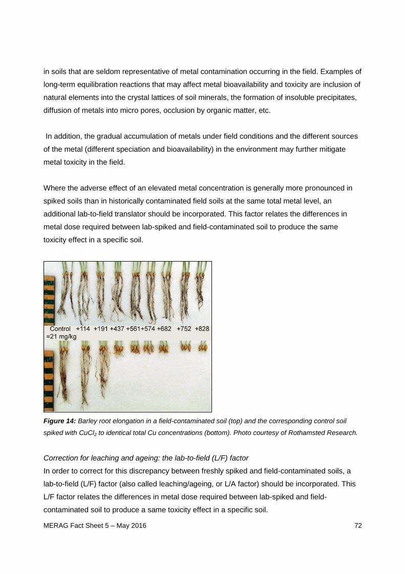
MERAG Fact Sheet 5 – May 2016
72
in soils that are seldom representative of metal contamination occurring in the field. Examples of
long-term equilibration reactions that may affect metal bioavailability and toxicity are inclusion of
natural elements into the crystal lattices of soil minerals, the formation of insoluble precipitates,
diffusion of metals into micro pores, occlusion by organic matter, etc.
In addition, the gradual accumulation of metals under field conditions and the different sources
of the metal (different speciation and bioavailability) in the environment may further mitigate
metal toxicity in the field.
Where the adverse effect of an elevated metal concentration is generally more pronounced in
spiked soils than in historically contaminated field soils at the same total metal level, an
additional lab-to-field translator should be incorporated. This factor relates the differences in
metal dose required between lab-spiked and field-contaminated soil to produce the same
toxicity effect in a specific soil.
Figure 14: Barley root elongation in a field-contaminated soil (top) and the corresponding control soil
spiked with CuCl2 to identical total Cu concentrations (bottom). Photo courtesy of Rothamsted Research.
Correction for leaching and ageing: the lab-to-field (L/F) factor
In order to correct for this discrepancy between freshly spiked and field-contaminated soils, a
lab-to-field (L/F) factor (also called leaching/ageing, or L/A factor) should be incorporated. This
L/F factor relates the differences in metal dose required between lab-spiked and field-
contaminated soil to produce a same toxicity effect in a specific soil.

MERAG Fact Sheet 5 – May 2016
73
This factor addresses the differences in toxicity between tests on soils spiked in the lab and
tests on field-contaminated soils using single species or micro-organisms, functional tests due
to differences in ionic strength, and ageing of metals in soil. This factor does not address
differences in effects between single-species lab test and multi-species tests (species
interactions). The influence of the latter is addressed by comparing micro/mesocosm or field
studies with the EQS based on single species/functional lab tests.
Guidelines for L/F calculation:
L/F factors should be calculated as a ratio between toxicity data generated from i) field-
contaminated soils or laboratory-spiked, leached and aged soils and ii) freshly spiked
soils.
A minimum ageing period after spiking can be metal-specific. The experience for Zn, Pb,
Cu and Ni indicated that 3 to 9 months is a good compromise between practical
considerations, while still allowing a realistic amount of time for slow
ageing/transformation reactions in soil. Longer ageing times may still result in a larger
L/F factor. Because kinetics of ageing may be metal specific, the minimum ageing period
required may be unique for different metals.
Soils should either be artificially leached before ageing or allow free drainage of
percolating rainwater in order to remove the excess salts (minerals?).
As natural metal background concentrations are already “aged”, the derivation of the L/F
factors should be based on added concentrations.
The L/F factors should be derived for a range of soils, ideally covering the relevant range
in soil properties and for several species, representing the three trophic levels.
The L/F factors are preferentially based on the ratio of EC50 because EC50 values
generally are a more statistically robust estimate compared to eg EC10. In cases less
than 50%, effect is observed at the largest dose tested, a ratio of lower effect levels
should be selected. EC10/EC20 values generally result in larger L/F factors due to larger
relative differences. Only if no ECx values are available is it acceptable to use NOEC
values.
In case no toxicity is observed at the highest dose tested in field conditions, in contrast
with that in a corresponding freshly amended soil, this information should not be ignored
and an unbounded (lower) estimate for the L/F factor should be derived as the ratio of
Lab-to-Field(L / F) factor =EC
x/NOECfield / aged ,add
ECx /NOECfreshlyspiked ,add

MERAG Fact Sheet 5 – May 2016
74
the highest dose tested under field conditions and the EC10,add (or NOEC) in the
corresponding freshly amended soil.
The selection of the most appropriate L/F factor is not straightforward and should be done in a
pragmatic and cautious but realistic way, for example by selecting one generic value situated at
the lower end of the spectrum. Preferentially, information on toxicity-based L/F factors should be
combined with information from changes in metal availability, eg based on changes in pore
water concentration or isotopic exchangeability (Ma et al 2006, 2013; Wendling et al 2009).
When no relationship can be found between soil properties and the lab-to-field factors, and/or
between organism and lab-to-field factor, all individual lab-to-field ratios should be aggregated
into a frequency distribution in order to derive a generic lab-to-field factor (eg Cu, Zn, Mo and
Pb, Table 6 and Example 8a). In cases where a significant relationship between soil properties
and the L/F factor is found, preference is given to derive soil-specific L/F factors for each ECx to
be corrected (Table 6 and Example 8b) (eg Ni and Co). It must be stressed that the L/F factor
should not be applied on ecotoxicity data collected in field contaminated or in spiked and aged
soils.
Metal L/F factor Key soil properties for
normalisation
Cu 2 eCEC*, Soil organic carbon
content, clay content, pH*
Ni 1-3 (increasing as a function of pH) eCEC
Pb 4 eCEC
Zn 3 eCEC, pH, background Co
Co 1-3.5 (increasing as a function of pH) eCEC
Mo 2 Clay, pH
Table 6: Lab-to-field factors and soil properties for normalisation for various metals as selected for
European risk assessment dossiers
*Where eCEC = effective cation exchange capacity, ie CEC at prevailing soil pH, as opposed to CEC
measured at a buffered pH, pH measured in 0.01 M CaCl2.
Example 8a: Derivation of L/F factor for Cu
Data availability:
1. Difference in Cu toxicity to plants, invertebrates and microbial processes between
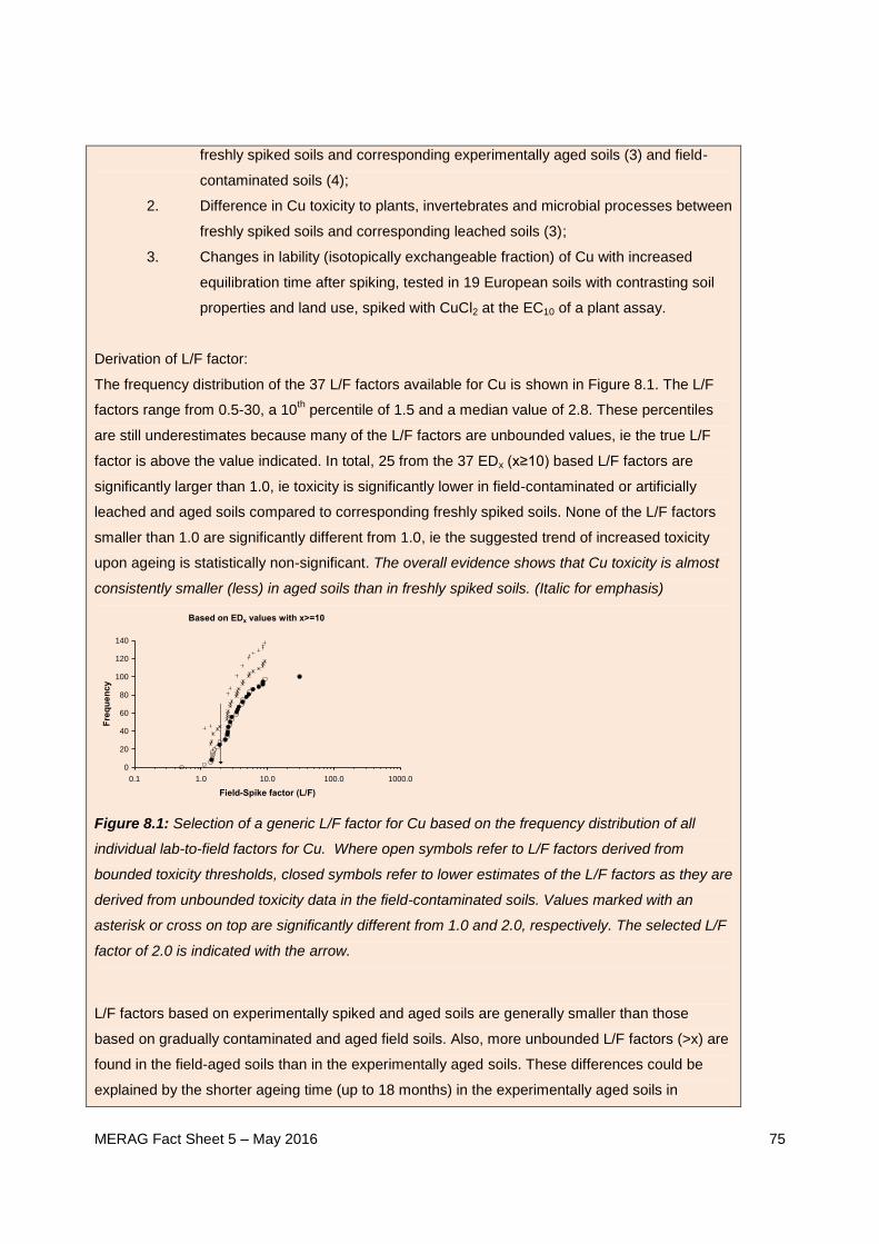
MERAG Fact Sheet 5 – May 2016
75
freshly spiked soils and corresponding experimentally aged soils (3) and field-
contaminated soils (4);
2. Difference in Cu toxicity to plants, invertebrates and microbial processes between
freshly spiked soils and corresponding leached soils (3);
3. Changes in lability (isotopically exchangeable fraction) of Cu with increased
equilibration time after spiking, tested in 19 European soils with contrasting soil
properties and land use, spiked with CuCl2 at the EC10 of a plant assay.
Derivation of L/F factor:
The frequency distribution of the 37 L/F factors available for Cu is shown in Figure 8.1. The L/F
factors range from 0.5-30, a 10th percentile of 1.5 and a median value of 2.8. These percentiles
are still underestimates because many of the L/F factors are unbounded values, ie the true L/F
factor is above the value indicated. In total, 25 from the 37 EDx (x≥10) based L/F factors are
significantly larger than 1.0, ie toxicity is significantly lower in field-contaminated or artificially
leached and aged soils compared to corresponding freshly spiked soils. None of the L/F factors
smaller than 1.0 are significantly different from 1.0, ie the suggested trend of increased toxicity
upon ageing is statistically non-significant. The overall evidence shows that Cu toxicity is almost
consistently smaller (less) in aged soils than in freshly spiked soils. (Italic for emphasis)
Figure 8.1: Selection of a generic L/F factor for Cu based on the frequency distribution of all
individual lab-to-field factors for Cu. Where open symbols refer to L/F factors derived from
bounded toxicity thresholds, closed symbols refer to lower estimates of the L/F factors as they are
derived from unbounded toxicity data in the field-contaminated soils. Values marked with an
asterisk or cross on top are significantly different from 1.0 and 2.0, respectively. The selected L/F
factor of 2.0 is indicated with the arrow.
L/F factors based on experimentally spiked and aged soils are generally smaller than those
based on gradually contaminated and aged field soils. Also, more unbounded L/F factors (>x) are
found in the field-aged soils than in the experimentally aged soils. These differences could be
explained by the shorter ageing time (up to 18 months) in the experimentally aged soils in
Based on EDx values with x>=10
0
20
40
60
80
100
120
140
0.1 1.0 10.0 100.0 1000.0
Field-Spike factor (L/F)
Fre
qu
en
cy

MERAG Fact Sheet 5 – May 2016
76
comparison to the ageing time ranging from 8 years to more than 70 years in the field-
contaminated soil. Further, differences in Cu availability between soils spiked once with a soluble
form of Cu and soils in which Cu is added slowly over time may explain the discrepancy between
laboratory and field-aged data. The L/F factor will therefore be based on the field data. The
experimentally aged data in the lab will be used as supporting evidence. There were no
significant correlations between these factors and age of the Cu contamination, soil type or type
of endpoint. This means that only a generic L/F factor can be used in the risk characterisation. A
generic L/F factor of 2.0 is proposed based on the following considerations:
1. The L/F factor of 2.0 is about equal to the product of the median factor found for
chemical fixation in several EU soils (factor 1.4) and the median factor for the
effects of leaching on the Cu toxicity thresholds (factor 1.3). The ionic strength
effect (leaching) is more important in soils with a low pH and CEC while the
ageing effect is more important in high pH soils. The combination of both effects
is similar overall for the soils tested.
2. This factor is about the 10-15th percentile of the field-contaminated soils and
about the 25th percentile of all individual factors (field-aged and experimentally
aged). In the field-contaminated soils, only 1 L/F factor is significantly smaller
(less) than the proposed generic factor of 2.0. Similarly, in the experimentally
aged soils, only 1 L/F factor is found that is smaller than the proposed generic
factor of 2.0. In other words, 5% of all generated L/F factors are significantly
lower than the proposed generic factor of 2.0. However, besides the factor the
absolute concentration should also be evaluated.
3.
This generic leaching-ageing factor of 2.0 will be used on all individual ECx,add values of tests
starting within 120 days after spiking to generate aged ECx,add values. For ECx,add values of tests
in soils that have equilibrated for more than 120 days after spiking, the L/A factor is 1.0.
Example 8b: Derivation of L/F factor for Ni
Data availability:
4. Difference in Ni toxicity to plants, invertebrates and microbial processes between
freshly spiked soils and 3 corresponding leached and experimentally aged soils.
5. Changes in lability (isotopically exchangeable fraction) of Cu with increased
equilibration time after spiking, tested in 16 European soils with contrasting soil
properties and land use, spiked with NiCl2 at the EC10 of a plant assay.
Derivation of L/F factor:

MERAG Fact Sheet 5 – May 2016
77
Clear differences in toxicity-based L/F factors for Ni were observed among the 3 different soils
tested (Figure 7.1). The fixation factor, calculated as the change in isotopically exchangeable
fraction of Ni in soil between 1 day after spiking and 540 days equilibrated in outdoor conditions,
ranged 0.7-4.0 with a median fixation factor of 1.0 and shows a clear increase with pH (Figure
8.2). It is proposed to use the fixation factor, derived from an empirical chemical model as the L/F
factor, ie L/F=1+exp(1.4(pH-7.0)
in which pH is the pH measured in CaCl2 0.01M. This equation is
calibrated on soil aged maximally 1.5 years and soil pH ranged between pH 3.6 and 7.7. That
empirical model predicts almost no ageing (L/F<1.2) up to pH 6 and L/F=2 at pH 7.0 and L/F=3 at
pH 7.5. The L/F factor estimated from the fixation factor only accounts for the changes in the
isotopically exchangeable pool, which is the fraction of the total that buffers the free metal ion
activity in solution. This factor is a conservative estimate for the changes in toxicity for Ni, as
shown in Figure 7.1. This factor will only be applied to ECx,add values of tests that are finished
within 120 days after spiking whereas this factor is 1.0 for all tests performed on soils aged >120
days before the end of the test.
Figure 8.2: The L/F factors for Ni based on toxicity (symbols) and the predicted factor changes in
labile pool of Ni in soil (line). Where open symbols are „unbounded‟ values and are a lower
estimate of the ageing factor. None of the ageing factors are significantly lower than that
predicted by the chemical model.
5.4.3 Normalisation for variation in soil properties
Metal toxicity thresholds for the same endpoint can vary up to two orders of magnitude among
different freshly spiked soil (Oorts et al 2006a; Rooney et al 2006; Criel et al 2008; Li et al 2009,
2010a; van Gestel et al 2011). Physico-chemical soil properties (eg pH, organic carbon
content, clay content and cation exchange capacity) can explain a significant part of the
variation in metal toxicity thresholds for plants, invertebrates and micro-organisms based on
(aqua regia-) total metal concentrations in soil and empirical regression models are derived,
covering a wide range of European soil types (Smolders et al 2009). Such regression models
can be used to correct the effects data for the differences in physico-chemical properties of the
1.0
10.0
100.0
3 4 5 6 7 8 9
soil pH (CaCl2 0.01M)
Ag
ein
g f
ac
tor
chemical model
toxicity ED50 based

MERAG Fact Sheet 5 – May 2016
78
soils tested and to normalise results towards specific conditions of a site of interest. By doing
so, these regressions allow for the derivation of site-specific environmental quality standards,
expressed as total metal concentration.
The derivation of normalisation models according to the regression approach is shown in Figure
15 and should take into account the following considerations:
The regression analysis is preferentially based on EC50 values because of the larger
robustness of this estimate compared to lower-effect levels in the similar trends
generally observed across the different effect levels (EC10, EC20, EC50,, …).
The ECx values should be linked with the soil properties (pH, organic carbon content,
clay content, eCEC) of the soils in which the test was performed. The effective CEC
(eCEC, ie CEC measured at prevailing soil pH) is preferred above the CEC measured at
a buffered pH because the former is a better estimate for the in situ conditions.
Regressions are preferably based on a log-log basis (except for pH as this is already a
log-transformed parameter). Shown as:
log(ECx) = intercept + slope * log(abioticfactor)
Although this is an empirical approach, it is strongly preferred that the models selected can be
mechanistically explained. In this aspect, mechanistic approaches, such as biotic ligand-type or
electrostatic models (Wang et al 2011, 2013), can be an effective validation of the correlations
observed in the empirical regression approach. For example, regressions with eCEC for cationic
metals can be explained by the higher sorption and hence lower bioavailability of cationic
metals with increasing eCEC of the soil. Final selection of the models should therefore be based
both on the statistical power (higher R2adj) of the regression model and the soil chemical
considerations.
1. In order to ensure maximal cross-species extrapolation, models should be
derived for a minimum of one species or endpoint for each relevant trophic level
of soil organisms (see also section 0).

MERAG Fact Sheet 5 – May 2016
79
Figure 15: General approach for derivation of toxicity derived normalisation models for toxicity to
terrestrial organisms.
Regression models used for accounting the effect of soil properties on metal bioavailability and
toxicity in soils have been derived for a wide range of European, Australian and Chinese soils in
the framework of corresponding risk assessment processes in these regions (Table 7, Table 8,
Example 9 and Figure 16). It must be noted that when several models are available for taking
into account the effect of soil properties on metal bioavailability and toxicity for the same
endpoint, they may have identified other soil properties as best predictor of metal toxicity for this
endpoint. So far, not all major soil types globally occurring are covered (tropical scenarios are
still missing). It is not yet known if the existing models are also applicable to such soils. A
summary of the abiotic soil factors selected for the normalisation models developed for
European soil is reported in Table 8.
Geographical region Metals Endpoints
Europe Cu, Ni, Pb, Zn, Co,
Mo, Ag
Plants (monocotyledon and dicotyledon)
Invertebrates (arthropod and annelid worm)
Microbial processes (nitrification and C-

MERAG Fact Sheet 5 – May 2016
80
respiration)
Australia Cu, Zn Plants (monocotyledon)
Microbial processes (nitrification and C-
respiration)
China Cu, Ni Plants (monocotyledon)
Invertebrates (annelid worm)
Microbial processes (nitrification)
Table 7: Global availability of normalisation models for metals.
Metal Organisms/Micro-
bial processes
Abiotic factors Reference
Ag Plants Organic C, pH and eCEC Langdon et al 2013
Invertebrates Organic C Langdon et al 2013
Microbial processes Organic C and eCEC Langdon et al 2014
Co Plants eCEC Mico et al 2008; Li et al 2009
Invertebrates eCEC De Schamphelaere et al 2008
Microbial processes eCEC Salpeteur et al 2007
Cu Plants eCEC Rooney et al 2006
Invertebrates eCEC Criel et al 2008
Microbial processes eCEC, Organic C, clay and
pH
Oorts et al 2006
Pb Plants eCEC Smolders et al 2011
Invertebrates eCEC Lanno 2012
Microbial processes eCEC Smolders et al 2011
Mo Plants pH and clay McGrath et al, 2010; Oorts et
al 2015
Invertebrates Clay Van Gestel et al 2011; Oorts
et al 2015
Microbial processes Clay Oorts et al 2015
Ni Plants eCEC Rooney et al 2007
Invertebrates eCEC Van Eeckhout et al 2005
Microbial processes eCEC Oorts et al 2006
Zn Plants pH and eCEC Smolders et al 2003
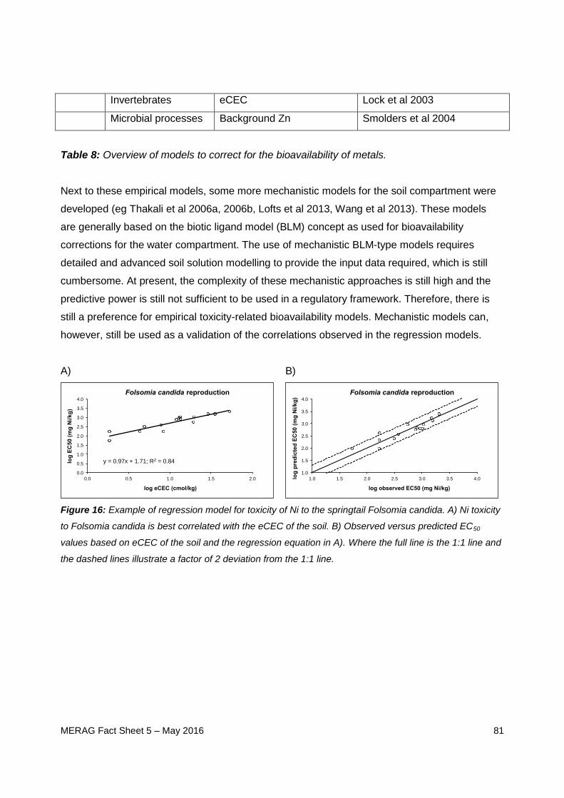
MERAG Fact Sheet 5 – May 2016
81
Invertebrates eCEC Lock et al 2003
Microbial processes Background Zn Smolders et al 2004
Table 8: Overview of models to correct for the bioavailability of metals.
Next to these empirical models, some more mechanistic models for the soil compartment were
developed (eg Thakali et al 2006a, 2006b, Lofts et al 2013, Wang et al 2013). These models
are generally based on the biotic ligand model (BLM) concept as used for bioavailability
corrections for the water compartment. The use of mechanistic BLM-type models requires
detailed and advanced soil solution modelling to provide the input data required, which is still
cumbersome. At present, the complexity of these mechanistic approaches is still high and the
predictive power is still not sufficient to be used in a regulatory framework. Therefore, there is
still a preference for empirical toxicity-related bioavailability models. Mechanistic models can,
however, still be used as a validation of the correlations observed in the regression models.
A) B)
Figure 16: Example of regression model for toxicity of Ni to the springtail Folsomia candida. A) Ni toxicity
to Folsomia candida is best correlated with the eCEC of the soil. B) Observed versus predicted EC50
values based on eCEC of the soil and the regression equation in A). Where the full line is the 1:1 line and
the dashed lines illustrate a factor of 2 deviation from the 1:1 line.
y = 0.97x + 1.71; R2 = 0.84
0.0
0.5
1.0
1.5
2.0
2.5
3.0
3.5
4.0
0.0 0.5 1.0 1.5 2.0
log
EC
50 (
mg
Ni/
kg
)
log eCEC (cmol/kg)
Folsomia candida reproduction
1.0
1.5
2.0
2.5
3.0
3.5
4.0
1.0 1.5 2.0 2.5 3.0 3.5 4.0 log
pre
dic
ted
EC
50 (
mg
Ni/k
g)
log observed EC50 (mg Ni/kg)
Folsomia candida reproduction

MERAG Fact Sheet 5 – May 2016
82
Example 9: Normalisation models for Cu
Various regression models are available for normalisation of Cu toxicity data for soil organisms (Table
9.1). For example, three different regression models exist for effect of soil properties on toxicity of Cu to
the microbial nitrification process in soil and all three models identified other soil properties as best related
with Cu toxicity: (1) eCEC (European model); (2) pH (Australian model); or (3) total calcium concentration
(Chinese model). These differences in the models can be due to either differences in soil types covered,
or also to potential differences in soil treatments (leaching and/or equilibration), methodology (eg (e)CEC
analysis), endpoints measured, etc.
Table 9.1 Soil properties selected for normalisation of Cu toxicity to terrestrial organisms.
Endpoint Geographical region Regression Reference
Eisenia fetida (earthworm)
reproduction
European soils eCEC Criel et al 2008
Folsomia candida (springtail)
reproduction
European soils eCEC Criel et al 2008
Potential nitrification rate European soils eCEC Oorts et al
2006a
Substrate-induced respiration European soils Organic carbon and
clay content
Oorts et al
2006a
Maize residue mineralisation European soils pH and eCEC Oorts et al
2006a
Barley root elongation European soils eCEC Rooney et al
2006
Tomato shoot yield European soils eCEC Rooney et al
2006
Substrate-induced nitrification Australian soils pH Broos et al 2007
Substrate-induced respiration Australian soils clay Broos et al 2007
Wheat shoot yield Australian soils CEC Warne et al
2008
Substrate-induced nitrification Chinese soils Total calcium
concentration
Li et al 2010b
Barley root elongation Chinese soils pH and organic carbon Li et al 2010a
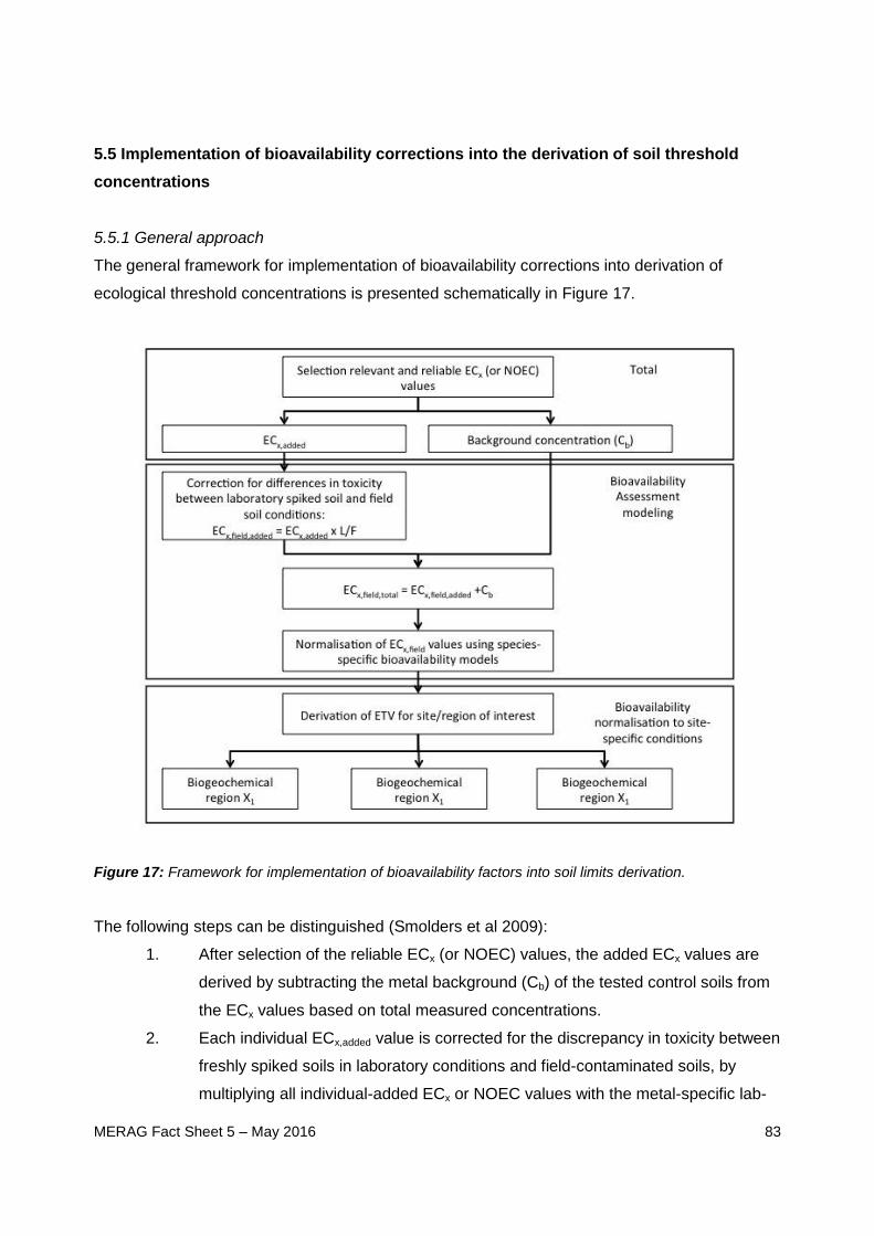
MERAG Fact Sheet 5 – May 2016
83
5.5 Implementation of bioavailability corrections into the derivation of soil threshold
concentrations
5.5.1 General approach
The general framework for implementation of bioavailability corrections into derivation of
ecological threshold concentrations is presented schematically in Figure 17.
Figure 17: Framework for implementation of bioavailability factors into soil limits derivation.
The following steps can be distinguished (Smolders et al 2009):
1. After selection of the reliable ECx (or NOEC) values, the added ECx values are
derived by subtracting the metal background (Cb) of the tested control soils from
the ECx values based on total measured concentrations.
2. Each individual ECx,added value is corrected for the discrepancy in toxicity between
freshly spiked soils in laboratory conditions and field-contaminated soils, by
multiplying all individual-added ECx or NOEC values with the metal-specific lab-
MERAG Fact Sheet 5 – May 2016
84
to-field (L/F) factor. When no relationship is found between soil properties and
the lab-to-field factor, one generic factor is used for all soils (eg, Cu, Zn, Pb).
When the lab-to-field factor depends on the soil properties (eg, pH for Ni and Co),
a specific lab-to-field factor is calculated for the soil properties of the soil tested
for each ECx in the database. In a total approach, the metal background
concentration from each individual test soil is then added again in order to
calculate the total “field” ECx or NOEC values. Previous steps should be omitted
for toxicity data from tests in field-contaminated or leached and long-term
equilibrated soils.
3. In the following step, the toxicity data are corrected for differences in metal
availability among soils. Normalising for the effect of soil properties allows the
calculation of a specific threshold concentration for the effect of metals to soil
organisms in the soil under investigation. Using the regression-model approach,
each total or added “field” ECx or NOEC value is normalised towards the soil
properties of a specific target soil, using the slope of the metal- and organism-
specific regression function (log-log based) and the following equation (Equation-
21):
(Eq-21)
Where “reference” is the soil for which the soil standard must be derived; “test” is the tested soil;
“abiotic factor” is the soil property with which toxicity is correlated; “slope” is the slope of the
selected log-log based regression equation. In cases where the L/F factor is dependent on soil
properties, the application of this factor will also affect the regression analysis between toxicity
thresholds and soil properties and the slope from regressions based on L/F corrected ECx
values should be used. If the L/F factor is a constant value for all soils, regressions can be
based on freshly spiked ECx values.
4. Finally, the environmental quality standard is derived based on the bioavailability-
corrected toxicity data. If, after normalisation, multiple data are available for the
same species or microbial process, a species/process mean value is calculated
as the geometric mean from all data for the most sensitive endpoint for each
species or process. This species/process mean approach is preferred for
ECx ,reference
=ECx ,test
abioticfactorreference
abioticfactortest
é
ë
êê
ù
û
úú
slope
MERAG Fact Sheet 5 – May 2016
85
normalised data, where the remaining variation among data for a given
species/process can be mainly attributed to intra-species variation in sensitivity.
This is, however, not the case for non-normalised data, where variation between
toxicity data is also caused by differences in bioavailability among soils.
Depending on the data available, the ETV can be derived using the AF or SSD
approach.
5.
Where possible, the complete effects data set should be normalised. This assumes that
reported effects data contain information on the abiotic soil bioavailability parameters of the test
system. When such information is not available, these data cannot be normalised and used for
the derivation of the bioavailability corrected soil threshold.
The final definition of an environmental limit obviously requires several regulatory choices, eg
on effect (choice of ECx) and protection level (choice of HCp) or on the organisms to be included
(Checkai et al 2014). The soil-specific limits in the European Union (EU) risk assessments were
all set using the sensitivity distribution of all species tested and the hazardous concentration for
5% of the species (HC5-50) estimated as the median fifth (5th) percentile of the cumulative
frequency distribution of the chronic NOEC or EC10 values from chronic toxicity tests for plants,
invertebrates and micro-organisms (European Chemicals Agency 2008).
Example 10: Impact of normalisation on EQS for Ni
Reliable chronic terrestrial toxicity data are available for Ni toxicity to 11 plant species, 6 invertebrate
species and 26 microbial endpoints, allowing the use of the SSD approach for derivation of an EQS.
Nickel toxicity to all terrestrial endpoints is best correlated with the eCEC of the soil. Without normalisation,
the toxicity values for varying soil properties, the HC5 (ie 95% protection level) is 24.7 mg Ni/kg.
Normalisation of toxicity values to a soil with low effective cation exchange capacity (eCEC = 5 cmolc/kg)
or to a soil with high effective cation exchange capacity (eCEC = 35 cmolc/kg) results in a HC5 of 10.3 and
94.4 mg Ni/kg soil, respectively.

MERAG Fact Sheet 5 – May 2016
86
Figure 10.1. The species sensitivity distribution for the effects of Ni on soil microbial processes, plants,
and invertebrates as affected by Ni bioavailability. The raw EC10 and NOEC values are shown as well as
the corresponding values corrected for bioavailability to a soil with low effective cation exchange capacity
(eCEC = 5 cmolc/kg) or to a soil with high effective cation exchange capacity (eCEC = 35 cmolc/kg)
(adapted from Smolders et al 2009).
5.5.2 Normalisation and cross-species extrapolation
Where bioavailability models are available, they exist mostly for a limited number of species
representing different trophic levels. Toxicity data generated for these species under different
abiotic conditions can be normalised to a common set of abiotic conditions as long as these soil
properties fall within the (geochemical) boundaries of the bioavailability model (eg range of
eCEC, organic matter, pH). For those species for which no specific bioavailability model has
been developed, it should be verified on a case-by-case basis whether the bioavailability model
of another species could be applied. Normalisation using bioavailability models and read-across
to other species for which no bioavailability model is available applies to any compartment
where a bioavailability model is available. It must be noted that lab-to-field correction factors are
derived based on the total weight of evidence and are not species- or endpoint-specific. Lab-to-
field factors are therefore applied on all toxicity data derived in recently spiked soils.
The application of normalisation models across species (full normalisation) is based on several
assumptions (eg, similar binding and uptake mechanisms, similar stability constants between
metals and the biotic ligands, similar site of action) and therefore the applicability across
0
20
40
60
80
100
1 10 100 1000 10000
Soil total Ni concentration (mg/kg)
Fre
qu
en
cy o
f N
OE
C/E
C1
0 v
alu
es (
%)
not normalised
normalised to eCEC=5
normalised to eCEC=35
5

MERAG Fact Sheet 5 – May 2016
87
species needs to be investigated. The evaluation of full read-across of the available
bioavailability models should include the following considerations:
Mode of Action (MOA). A similar mode of action across species is a qualitative
argument for read-across. In principle, it is very difficult to know the „mode of action‟ of a
metal ion for a particular species, and certainly one where only limited data are
available. Even in circumstances where the same „mode of action‟ is likely, there
remains the uncertainty of whether the quantitative changes in physiological response to
changes in metal ion availability will be identical between species.
Physiological similarities of the species. Similarity of species can be used as
justification for use of a particular models, eg use of a model derived for one terrestrial
arthropod species for normalisation of toxicity data of other arthropod species. Such
extrapolation is widely used in environmental risk assessment for practical reasons, but
it is not without uncertainties and these need to be considered in drawing conclusions.
Clearly, there is a limit to how far such an extrapolation can be made before validity of
the extrapolation should be confirmed. For read-across of bioavailability models among
terrestrial organisms, the following rules should be taken into account:
o Read-across is only accepted within the same trophic level (plants, invertebrates
or micro-organisms). Extrapolation to a different trophic level is hence not
allowed.
o For terrestrial invertebrates, a distinction is made between hard-bodied (eg,
arthropods) and soft-bodied (eg, annelid worms) organisms and read-across
between these 2 groups is not recommended because of differences in the
importance of dermal and oral exposure route between these groups of
organisms.
o Similarly, a distinction is generally made between microbial processes related to
the nitrogen cycle (eg nitrification, N mineralisation) and the carbon cycle (eg
respiration) in soil. Read-across between these 2 groups is also not
recommended because of the larger functional redundancy for processes related
to the C-cycle.
o In case several potential models are available for read-across and there is no
clear preference based on mode of action or physiognomy (eg for plants), the
model with the smallest correction factors (ie the smallest slopes in case of
regression models) should be selected as a conservative approach.
MERAG Fact Sheet 5 – May 2016
88
Decrease in intra-species variability (eg max/min ratio) in ECx values after
normalisation. Normalisation of the individual ECx data towards specific soil properties
should significantly reduce the within species-variation in ECx values. This is a
quantitative illustration of the adequacy of the models and the significance of soil
properties in controlling the bioavailability and toxicity of metals to soil organisms and
further demonstrates the importance of normalisation of the toxicity data and separating
the biological variation from the variation in metal availability because of varying soil
properties.
Similarity of the bioavailability models across species and endpoints tested. In
case where one metal has the same abiotic factors selected for normalisation of toxicity
values for all species and functions tested (eg eCEC for Co and Ni) and if all regression
slopes are very similar, these factors show that the relationships are consistent, and that
the models can be used across species. In such cases, the choice of a particular
relationship is not critical because the other relationships available will yield similar
results. Therefore, even if a relationship would be incorrectly applied to a species in the
database, this would not make a difference, because the “correct” relationship would be
very similar to the one that was in fact used.
Spot-check validations for other organisms (ie few ecotoxicity data from tests
performed under different geochemical conditions for a range of key soil parameters (eg
eCEC).
Field or mesocosm validation.
Understanding of sensitive ecologically relevant species.
The level of checking, eg testing of additional taxa to confirm applicability of the models, would
be determined on a case by case basis taking into account the level of uncertainty in the
extrapolations, and the extent to which it is necessary to reduce uncertainty. Considering that
sensitive species are generally driving the assessment, it should be demonstrated that the
developed/validated bioavailability models could be applied to the most sensitive
species/taxonomic groups of the database. It is also needed to consider if certain keystone
species or important groups of organisms/trophic levels are missing.
At present, no bioavailability models are available for acute toxicity endpoints and therefore it is
not possible to use such acute bioavailability models to normalise chronic data. In case such
models would be available, their use should be considered with great care. Such normalisation
is only allowed in case the predictive capacity of these acute models is sufficient for estimating

MERAG Fact Sheet 5 – May 2016
89
chronic toxicity data. In the case of poor predictive power of the acute models towards chronic
toxicity data, the acute model could only be used to normalise the acute toxicity data. The
derivation of chronic effects levels could then be derived from the normalised acute toxicity data
using an acute to chronic ratio.
If full read-across is justified, the next step consists of applying the bioavailability model across
species of similar trophic levels (eg applying the Folsomia candida bioavailability model for
normalisation of the toxicity data from other arthropods …) towards a specific set of
geochemical conditions. The bioavailability models normalise the effect concentrations (ECx
values) of the metal for each species‟ endpoint and therefore retain the intrinsic metal
sensitivities of the different species and endpoints. The species-specific normalised geomean
ECx values for the most sensitive endpoints are then used to derive the soil limit concentrations.
In case read-across is only justified for some species and not for others (eg unexplained
significant increase in variability after normalisation or different mode of action), an alternative
conservative approach should be developed. In this approach, the bioavailability models are
only applied to those species within the trophic level for which the application can be justified.
For those species for which application of a bioavailability model related to their trophic level
cannot be justified, either all data, or the worst-case (ie lowest) ECx values, are selected for
derivation of the soil limit concentrations. This decision should be made on a case-by-case
basis and should consider eg the intra-species variation in toxicity data before and after
normalisation.
Example 11: Full cross-species normalisation for Cu
Seven chronic regression models are available for effect of Cu to different taxonomic groups: two different
bioavailability models for higher plants belonging to different taxonomic groups, ie, H. vulgare
(monocotyledon) and L. esculentum (dicotyledon); two different bioavailability models for invertebrates
belonging to different taxonomic groups, ie, E. fetida (soft bodied) and F. candida (hard bodied); three
different bioavailability models are available for different microbial processes, ie nitrification, substrate-
induced respiration and plant residue mineralisation.
For those organisms or endpoints without a specific regression model, the most conservative model (ie,
lowest slope) from similar species within the same trophic level is selected. The max/min ratios for the
normalised toxicity data show in most cases to be smaller than a factor of 15, while originally a
considerably higher intra-species variability (up to 73) was observed for the non-normalised NOEC data
(Figure 10.1). This results in a reduction in intraspecies variability up to 78% for the microbial processes,

MERAG Fact Sheet 5 – May 2016
90
up to 66% for the invertebrates, and up to 60% for the higher plants. However, in some cases the max/min
ratio is higher after normalisation. It must be stressed that in such cases the absolute value of the intra-
species variability after normalisation is still very low, ie, 2.9 for A. sativa, 4.7 for E. andrei, 1.4 for L.
rubellus, and 8.0 for glutamic acid. Application of the chronic regressions therefore seems to reduce the
uncertainty associated with the effects assessment and can be applied for setting an ecologically more
relevant EQS.
Figure 11.1. The intra-species variability (expressed as max/min ratios) of the normalised and non-
normalised EC10 and NOEC for Cu toxicity to terrestrial organisms, using the terrestrial chronic
bioavailability regression models.
Example 12: Partial cross-species normalisation for Pb
In the European risk assessment dossier for Pb, significant regression models are available for plants
(shoot yield of tomato and barley), earthworm reproduction and microbial nitrification. Although the effect
of soil properties on toxicity of Pb to arthropods (Folsomia candida) and microbial respiration processes
were also studied, no significant correlation between Pb toxicity and soil properties was observed.
Application of the regression models for plants, earthworms and nitrification to toxicity data for other
species or endpoints within the same trophic level, did not show a consistent reduction in the intra-species
variation of NOEC or EC10 values (as shown by the maximum/minimum ratio (Figure 12.1).
With the exception for Zea mays, the intra-species variation decreased for all plants after normalisation.
Changes were, however, not large. Although the intra-species for Zea mays slightly increased after
normalisation, its absolute value was still very small compared to all other species. The intra-species
variation for Eisenia fetida and the nitrification process was strongly reduced after normalisation. However,
the opposite trend was observed for toxicity data for Folsomia candida and respiration processes. Based
0
10
20
30
40
50
60
70
80
micro
bial b
iom
ass
subs
trate
indu
ced
resp
iratio
n
glut
amic a
cid
deco
mpos
ition
mai
ze re
spira
tion
resp
iratio
n
nitri
ficat
ion
N-m
inera
lisat
ion
Avena
sat
iva
Hor
deum
vulgar
e
Lyco
pers
icon
esc
ulen
tum
Cog
netti
a sp
hagn
etor
um
Eisen
ia a
ndre
i
Eisen
ia fe
tida
Lum
bricus
rube
llus
Folso
mia
can
dida
Folso
mia
fim
etaria
Isot
oma
virid
is
max/m
in r
atio
non-normalised
normalised

MERAG Fact Sheet 5 – May 2016
91
on these observations, normalisation models are not applicable for data for arthropods (Folsomia) and
respiration processes (both basal respiration and substrate-induced respiration). Therefore, non-
normalised toxicity data for these endpoints are used for the derivation of an EQS, while toxicity data for
other endpoint (toxicity to plants, annelid worms and microbial nitrification process) were normalised
towards specific soil conditions.
Because the intra-species variation in toxicity values for the effect of Pb to soil organisms was large
compared to the inter-species variation in toxicity, it was assumed that overrepresentation of certain
species in the cumulative distribution will not create a significant bias towards higher or lower toxicity
thresholds. Therefore, all individual toxicity data (either normalised or not) were included in the SSD for
direct effects of Pb to soil organisms.
Figure 12.1 The intra-species variability (expressed as max/min ratios) before and after normalization of
the toxicity data for effects of Pb to terrestrial organisms with the terrestrial chronic bioavailability
regression models. (Spelling of “normalisation” twice in Fig. 12.1 has to be done)
5.5.3 Validation of bioavailability-corrected soil quality standards
Few soil limit values for metals used across the world for environmental and ecosystem
protection have been validated. Validation in this sense means an assessment in the field in
order to establish whether the protection goal for which the limit value was set is achieved. A
study for the UK Environment Agency assessed several soil quality standards in terms of their
effectiveness and practicality on a range of soils (Nicholson et al 2008). The „effectiveness‟ was
gauged in terms of whether the limit values were predictive of risk conditions for soils for which
secondary data on soil biological process were also available.
0
20
40
60
80
100
120
140
160
180
200
Tricumaes
vum
Lactucasava
Zeam
ays
Loliumperenne
Echinochloacrusgalli
Lycopersiconesculentum
Hordeumvulgare
Oryzasava
Eiseniafeda
Folsomiacandida
N-mineraliza
on
Nitrificaon
Basalrespiraon
Substrateinducedrespira
on
Maxim
um/m
inim
umra
o
Beforenormaliza on
A ernormaliza on

MERAG Fact Sheet 5 – May 2016
92
In total, 95 field sites were identified with soil data on metal concentrations, soil physico-
chemical properties and biological effects indicating „soil health‟. These biological effects include
a significant (p<0.05) reduction in crop yield, reduction in biomass, increase in respiration rate,
or reduction in vertebrate numbers compared to a reference plot or exceeding Cd concentration
in wheat grain.
Site-specific soil quality standards, based on lab-to-field correction factors and normalisation
equations reported in the European Risk Assessment dossiers for Zn, Cu, Ni, Cd and Pb
correctly assessed the absence or presence of risks in 72 of the 95 soils tested. These soil
quality standards were under-protective of only six soils, ie the actual soil metal concentrations
in these soils were below the quality standard but a significant negative biological effect was
observed, while they were over-protective, ie effect predicted but not observed, for 17 soils. Soil
quality standards considering bioavailability performed better than generic soil quality standards
that do not take into account metal bioavailability in soil. These results therefore illustrate the
validity of the lab-to-field correction factors and normalisation regression models applied.
5.5.4 Application in a risk assessment context
For the application of toxicity-related bioavailability models in a risk assessment context, a
tiered approach for the incorporation of bioavailability in risk assessment procedures is
proposed. At each tier, exposure concentrations should be compared to the environmental
threshold value. In case this comparison leads to risks, more site-specific approaches should be
developed based on site-specific information on soil properties (Figure 18).

MERAG Fact Sheet 5 – May 2016
93
Figure 18: Tiered approach for refinement of soil ETV values.
Information on the main abiotic factors controlling metal bioavailability needs to be collected in
order to apply the toxicity models. This type of data can be obtained from existing monitoring
databases or from specifically tailored monitoring campaigns. As a first tier, the realistic worst-
case scenario can be used as a reference scenario, providing a soil limit value corresponding to
a maximum bioavailability. Care should, however, be taken that the combination soil properties
that maximise the bioavailability do not result in an unrealistic scenario ignoring the covariance
among soil properties in natural soils. Therefore, where different parameters influence the
bioavailability of the metal (eg Cu, Zn, Mo), the reference scenario should as far as possible be
a realistic combination of the relevant soil parameters. It is therefore recommended that a
reasonable worst-case ETV for a generic first tier local risk assessment is derived based on a
distribution of normalised ETVs for a representative range of sites for the region/continent of
interest. In case bioavailability models for a metal are all based on the same single soil property
(eg eCEC for Ni and Co), worst-case estimates on the soil properties or the resulting ETV
values result in the same reasonable worst-case ETV value.

MERAG Fact Sheet 5 – May 2016
94
Example 13: Selection of EQS for molybdenum
Mo toxicity in soil decreases, (= increase of the EQS) when clay content increases and pH of the soil
decreases. The 5th percentile (HC5) of EC10 and NOEC values normalised to a reasonable worst-case clay
content (ie 10th percentile) and pH (ie 90
th percentile) in arable soils across Europe is 1.0 mg Mo/kg dw
(Table 13.1). This value is significantly different from the reasonable worst-case EQS as calculated based
on the 10th percentile of the distribution of HC5 values normalised to all individual clay-pH combinations in
the same dataset for arable soil in Europe (10.5 mg Mo/kg dw). When sufficient actual site-specific EQS
data are available, the latter approach is therefore strongly preferred for derivation of a reasonable worst-
case EQS. The value of 1.0 mg Mo/kg corresponds to <1st percentile of all predicted site-specific HC5
values across Europe, and can therefore be considered as overprotective. Soil pH and clay content are
generally positively correlated and therefore soils with high pH (90th percentile) and low clay content (10
th
percentile) do not represent a realistic worst-case scenario.
Further information on the physico-chemical properties for the site of interest yields further refinement of
the EQS. The EQS for the best corresponding biogeochemical region can be either over- or
underprotective depending on the actual soil properties of the site.
Table 13.1: Tiered approach for calculation of EQS for Mo in a loamy soil with pH 7.0 and 25% clay. EQS
is calculated as the 5th percentile of EC10 and NOEC values. Reasonable worst-case estimates for PNEC
for Mo in European arable soil.
Approach EQS
(mg Mo/kg)
Reasonable worst case EQS based on reasonable worst-case assumptions
for clay and pH in Europe (data from GEMAS database, Reimann et al 2014)
1.0
Reasonable worst case EQS based on distribution of site-specific EQS
values across Europe
10.5
EQS for standard loamy soil (biogeochemical region approach) 30.6
EQS calculated for soil-specific information (pH 7.0 and 25% clay) 22.4
5.5.5 Relative importance of dietary route for metals in soils
The dietary route is only relevant for terrestrial invertebrates that may take up contaminated soil
or food via the oral route. Although earthworms ingest significant amounts of soil, it is concluded
that for metals the dermal route is the uptake route of importance (Vijver et al 2003). Moreover,
oral exposure to soils contaminated with the metal of concern is intrinsically included in the
MERAG Fact Sheet 5 – May 2016
95
assessment. As for the sediment compartment, the dietary exposure could be underestimated
for those species getting additional uncontaminated food during chronic toxicity testing and
further scientific research is needed to assess the relative importance of the dietary route and
its consequences for risk assessment purposes. However, the aqueous phase of the soil (soil
pore water) is considered the main exposure route for most soil invertebrates (Ardestani et al
2014). Because plants and micro-organisms are also exposed via the soil pore water, the
dietary exposure route may be considered of lower importance in a risk assessment of metal
toxicity to soil organisms.
5.5.6 Soil threshold calculator tools
All bioavailability correction models and the data selected for the EU REACH dossiers
(Registration, Evaluation, Authorisation for a range of metals (Cu, Ni, Zn, Pb, Cd, Co and Mo)
are compiled into a user-friendly tool, available at http://www.arche-consulting.be/metal-csa-
toolbox/soil-pnec-calculator/. This spreadsheet calculates the predicted ecological risks of
metals in soils, based on their Predicted No-Effect Concentrations (PNEC) to soil organisms, as
derived in the EU REACH dossiers for these metals. PNEC values are calculated as the 5th
percentile of the SSD divided by an additional assessment factor and are expressed as (aqua
regia) total metal concentrations in soil. PNEC values are derived for different levels of
refinement, depending on i) the availability of correction factors for the metal of interest and ii)
the available data on soil properties for the site of interest. The input soil parameters required
for calculation of site-specific PNEC values are dependent upon the metal under consideration
(Ta), and are generally readily available soil parameters likely to be determined in routine soil
analyses. In case no site-specific data are available, but the general soil type of the site is
known, one of six standard soil types ('ecoregions') can be assigned in order to still derive a
general PNEC value for this soil type.
A similar interactive (Excel) calculation spreadsheet is available for calculation of Ecological
Investigation Levels for metals under the National Environmental Protection (Assessment of
Site Contamination) Measure in Australia (http://www.scew.gov.au/node/941).

MERAG Fact Sheet 5 – May 2016
96
6. REFERENCES
Ahlf W, Drost W, Heise S (2009). Incorporation of metal bioavailability into regulatory
frameworks-metal exposure in water and sediment. Journal of Soils and Sediments, 9 (5), pp
411-419.
Alsop DH, Wood CM (2000). Kinetic analysis of zinc accumulation in the gills of juvenile rainbow
trout: Effects of zinc acclimation and implications for biotic ligand modeling.
Environ.Toxicol.Chem., 19 (7), 1911-1918.
Allison JD, and Allison TL (2005). Partition coefficients for metals in surface water, soil and
waste. U.S. Environmental Protection Agency, Washington, DC, 2005.
Ankley GT (1996). Evaluation of metal/acid-volatile sulfide relationships in the prediction of
metal bioaccumulation by benthic macroinvertebrates. Environ. Toxicol. Chem., 15 (12), 2138-
2146.
Antunes PMC, Hale BA, Ryan AC (2007). Toxicity versus accumulation for barley plants
exposed to copper in the presence of metal buffers: progress towards development of a
terrestrial biotic ligand model. Environ. Toxicol. Chem., 26 (11), 2282–2289.
Ardestani MM, van Straalen NM, van Gestel CAM.,(2014). The relationship between metal
toxicity and biotic ligand binding affinities in aquatic and soil organisms: a review.
Environ.Pollut., 195, 133-147.
Bell RA and Kramer JR (1999). Structural chemistry and geochemistry of silver-sulfur
compounds: a critical review. Environ. Toxicol. Chem., 18, 9-22.
Bianchini A, Bowles KC, Brauner CJ, Gorsuch JW, Kramer JR and Wood C (2002). Evaluation
of the effect of reactive sulfide on the acute toxicity of silver (I) to Daphnia magna. Part 2:
Toxicity results. Environ. Toxicol. Chem., 21, 1294-1300.
Bio-met (2011). Bio-met bioavailability tool. Available at http:/www.bio-met.net (after
registration).
MERAG Fact Sheet 5 – May 2016
97
Bo, Pan, et al (2016) Predicting copper acute toxicity to cyprinus carpio based on biotic ligand
model. In preparation.
Borgmann U (2003). Derivation of cause-effect based sediment quality guidelines. Canadian
Journal of Fisheries and Aquatic Sciences, 60(3), 352-360.
Borgmann U, Norwood WP, Reynoldson TB, Rosa F (2001). Identifying cause in sediment
assessments: bioavailability and the sediment quality triad. Canadian Journal of Fisheries and
Aquatic Sciences, 58(5), 950-960.
Bossuyt BTA, De Schamphelaere KAC, Janssen CR (2004). Using the biotic ligand model for
predicting the acute sensitivity of cladoceran dominated communities to copper in natural
surface waters. Environ. Sci. Tech., 38(19), 5030 -5037.
Brooks ML, Boese CJ, Meyer JS (2006). Complexation and time-dependent accumulation of
copper by larval fathead minnows (Pimephales promelas): Implications for modeling toxicity.
Aquat.Toxicol. 78 (1), 42-49.
Broos K, Warne MSJ, ,Heemsbergen DA, Stevens D, Barnes MB, Correll RL, McLaughlin MJ
(2007). Soil factors controlling the toxicity of copper and zinc to microbial processes in
Australian soils. Environ. Toxicol. Chem., 26, 583-590.
Bury NR, Shaw J, Glover C, Hogstrand C (2002). Derivation of a toxicity-based model to predict
how water chemistry influences silver toxicity to invertebrates. Comp.Biochem.Physiol. Part C,
133 (1-2), 259-270.
Campbell PGC (1995). Interactions between trace metals and aquatic organisms: a critique of
the Free-ion Activity Model. In: Tessier A, Turner DR (eds), Metal Speciation in Aquatic
Systems. John Wiley, New York, New York, pp. 45-102.
Casares MV, de Cabo LI, Seoane RS, Natale OE, Castro Ríos M, Weigandt C, de Iorio AF
(2012). Measured Copper Toxicity to Cnesterodon decemmaculatus (Pisces: Poeciliidae) and
Predicted by Biotic Ligand Model in Pilcomayo River Water: A Step for a Cross-Fish-Species
Extrapolation. J Toxicol, 2012, 849-315.

MERAG Fact Sheet 5 – May 2016
98
Chapman PM (2000). The sediment quality triad: then, now and tomorrow. Int. J. Environ.
Pollut., 13,1-6
Chapman PM (2001). Utility and relevance of aquatic oligochaetes in Ecological Risk
Assessment. Hydrobiologia, 463, 149-169.
Checkai R, Van Genderen E, Sousa JP, Stephenson G, Smolders E (2014). Deriving site-
specific clean-up criteria to protect ecological receptors (plants and soil invertebrates) exposed
to metal or metalloid soil contaminants via the direct contact exposure pathway. Integrated
Environmental Assessment and Management, 10 (3), 346-357.
Chen BC, Chen WY, Liao CM (2009). A biotic ligand model-based toxicodynamic approach to
predict arsenic toxicity to tilapia gills in cultural ponds. Ecotoxicology, 18(3), 377-383.
Chen S, Wang WB (2014). Study on Environmental Pollution Problems in the Copper Industry.
Advanced Materials Research, 889, 1600-1603.
Clifford M, McGeer JC (2009). Development of a biotic ligand model for the acute toxicity of zinc
to Daphnia pulex in soft waters. Aquat.Toxicol., 91(1), 26-32.
Clifford M, McGeer JC (2010). Development of a biotic ligand model to predict the acute toxicity
of cadmium to Daphnia pulex. Aquat.Toxicol., 98(1), 1-7.
Constantino C, Scrimshaw M, Comber S, Churchley J (2011). An evaluation of biotic ligand
model predicting acute copper toxicity to Daphnia magna in wastewater effluent.
Environ.Toxicol.Chem., 30(4), 852-860.
Costello DM, Burton GA, Hammerschmidt CR, Taulbee WK (2012). Evaluating the performance
of diffusive gradients in thin films for predicting Ni sediment toxicity. Environ. Sci. Technol., 46,
10239-10246.
Costello DM, Burton GA, Hammerschmidt CR, Rogevich EC, Schlekat CE (2011). Nickel phase
partitioning and toxicity in field deployed sediments. Environ. Sci.Technol., 45, 5798-5805.
Criel P, Lock K, Van Eeckhout H, Oorts K, Smolders E, Janssen CR (2008). Influence of soil
properties on copper toxicity for two soil invertebrates. Environ. Tox. Chem., 27, 1748-1755.
MERAG Fact Sheet 5 – May 2016
99
T. Crommentuijn et al (1997). Maximum permissible concentrations and negligible
concentrations for metals, taking background concentrations into account, Netherlands, Institute
of Public Health and the Environment, RIVM, Bilthoven, RIVM report No. 601501001, 1997.
David M, Perceval O, Batty J, Rodriguez RJ, Niebeek G, Delbeke K, Van Assche F, Merrington
G, Schlekat C (2011). Workshop on metal bioavailability under the water framework directive:
policy, science and implementation of regulatory tools. Workshop Report.
De Jonge M, Blust R, Bervoets L (2010). The relation between acid volatile sulfides (AVS) and
metal accumulation in aquatic invertebrates : implications of feeding behavior and ecology.
Environ. Pollut., 158, 1381-1391.
De Jonge M, Dreesen F, De Paepe J, Blust R and Bervoets L (2009). Do acid volatile sulfides
(AVS) influence the accumulation of sediment-bound metals to benthic invertebrates under
national field conditions. Environmental Science and Technology., 43, 4510-4516.
De Jonge M, Eyckmans M, Blust R, Bervoets L (2011). Are accumulated sulfide-bound metals
metobolically available in the benthic oligochaete Tubifex tubifex. Environmental Science and
Technology, 45, 3131-3137.
De Schamphelaere KAC, and Janssen CR (2004b). Effects of chronic dietary copper exposure
on growth and reproduction of Daphnia magna. Environ. Tox. Chem., 23, 2038-2047.
De Schamphelaere KAC and Janssen CR (2005). Development of a chronic BLM for fish. Final
report.
De Schamphelaere KAC and Janssen CR (2006). Bioavailability models for predicting copper
toxicity to freshwater green micro-algae as a function of water chemistry. Environmental
Science and Technology, 40, 4514-4522.
De Schamphelaere KAC, Lofts S, Janssen CR (2005). Bioavailability models for predicting
acute and chronic toxicity of zinc to algae, daphnids and fish in natural surface waters. Environ.
Tox. Chem., 24, 1190-1197.

MERAG Fact Sheet 5 – May 2016
100
De Schamphelaere KAC (2003). Bioavailability models for predicting copper toxicity to
freshwater organisms. Thesis submitted in fulfillment of the requirements for the degree of
Doctor in Applied Biological Sciences. Ghent University, Belgium. 292 p.
De Schamphelaere KAC and Janssen CR (2004a). Development and field validation of a biotic
ligand model predicting chronic copper toxicity to Daphnia magna. Environ. Tox. Chem., 23,
1365-1375.
De Schamphelaere KAC, Bossuyt BTA, Janssen CR (2007). Variability of the protective effect
of sodium on the acute toxicity of copper to freshwater cladocerans. Environ. Toxicol. Chem.,
26(3), 535-542.
De Schamphelaere KAC, Forrez I, Dierckens K, Sorgeloos P, Janssen CR (2007). Chronic
toxicity of dietary copper to Daphnia magna. Aquatic Toxicology, 81,409-418.
De Schamphelaere KAC, Heijerick DG, Janssen CR (2002). Refinement and field validation of a
biotic ligand model predicting acute copper toxicity to Daphnia magna. Comp.Biochem.Physiol.
Part C 133, 243-258.
De Schamphelaere KAC, Heijerick DG, Janssen CR (2006). Cross–phylum comparison of a
chronic biotic ligand model to predict chronic toxicity of copper to a freshwater rotifer,
Brachionus calyciflorus. Ecotoxicology and Environmental Safety, 63, 189-195.
De Schamphelaere KAC, Heijerick DG, Janssen CR (2003a). Development and validation of
biotic ligand models for predicting chronic toxicity to fish, Daphnia and algae. Final report on
project ZEH-WA-1, for the International Lead and Zinc Research Organisation (ILZRO),
February 2003.
De Schamphelaere KAC, Heijerick DG, Janssen CR (2003b). Cross-phylum comparison of a
chronic biotic ligand model to predict chronic toxicity of copper to a freshwater rotifer,
Brachionus calyciflorus (Pallas). Ecotoxicology and Environmental Safety, 63, 189-195.
De Schamphelaere KAC and Janssen CR (2002). A biotic ligand model predicting acute copper
toxicity for Daphnia magna: The effects of calcium, magnesium, sodium, potassium, and pH.
Environ. Sci. Technol., 36(1), 48-54.
MERAG Fact Sheet 5 – May 2016
101
De Schamphelaere KAC and Janssen CR (2004). Bioavailability and chronic toxicity of zinc to
juvenile rainbow trout (Oncorhynchus mykiss): Comparison with other fish species and
development of a biotic ligand model. Environ. Sci. Technol., 38(23), 6201-6209.
De Schamphelaere KAC, Nys C, Janssen C (2014). Toxicity of lead (Pb) to freshwater green
algae: development and validation of a bioavailability model and inter-species sensitivity
comparison. Aquatic Toxicology, 155, 348-359.
De Schamphelaere KAC, van Laer L, Deleebeeck NME, Muyssen BTA, Degryse F, Smolders E
et al (2006). Nickel speciation and ecotoxicity in european natural surface waters: development,
refinement and validation of bioavailability models. Report prepared for the Nickel Producers
Environmental Research Association (NiPERA), Durham, NC (USA). Gent University,
Laboratory of Environmental Toxicology and Aquatic Ecology, Gent, Belgium.
De Schamphelaere KAC, Vasconcelos FM, Allen HE, Janssen CR (2004). The effect of
dissolved organic matter source on acute copper toxicity to Daphnia magna. Environ.
Tox.Chem., 23(5), 1248-1255.
De Schamphelaere KAC, Nguyen LTH, Janssen CR (2008). Bioavailability and aging of cobalt
in soils: invertebrate toxicity testing. Final report submitted to Cobalt Development Institute.
De Schamphelaere KAC, Vasconcelos FM, Heijerick DG, Tack F, Delbeke K, Allen HE,
Janssen CR (2003c). Development and field validation of a predictive copper toxicity model for
the green alga Pseudokirchneriella subcapitata. Environ. Tox. Chem., 22(10), 2454–2465.
DeForest DK and Meyer SJ (2015). Critical review: toxicity of dietborne metals to aquatic
organisms. Critical Reviews in Environmental Science and Technology 45(11), 1176-
1241.
Degryse F, Buekers J, Smolders E,,(2004). "Radio-labile cadmium and zinc in soils as affected
by pH and source of contamination." European Journal of Soil Science, 55(1), 113-121.
Deleebeeck NME, De Laender F, De Schamphelaere KAC, Chepurnov V, Vyverman W,
Janssen CR (2009b). A single bioavailability model can accurately predict Ni toxicity to green
microalgae in soft and hard surface waters. Water Research 43, 1935-1947

MERAG Fact Sheet 5 – May 2016
102
Deleebeeck NME, De Schamphelaere KAC, Muyssen BTA, De Laender F, Janssen CR (2006).
Ni toxicity to soft vs. hard water organisms: a comparison of sensitivity and bioavailability.
Laboratory of Environmental Toxicology and Aquatic Ecology, Ghent University, Belgium, Draft
final report, 2006.
Deleebeeck NME, De Schamphelaere KAC, Heijerick DH, Bossuyt BTA, Janssen CR (2008).
The acute toxicity of nickel to Daphnia magna: Predictive capacity of bioavailability models in
artificial and natural waters, Ecotoxicology and Environmental Safety, 70, 67-78.
Deleebeeck NME, De Schamphelaere KAC, Janssen CR (2007b). A bioavailability model
predicting the toxicity of nickel to rainbow trout (Oncorhynchus mykiss) and fathead minnow
(Pimephales promelas) in synthetic and natural waters. Ecotoxicology and Environmental
Safety, 67, 1-13.
Deleebeeck NME, De Schamphelaere KAC, Janssen CR (2009a). Modeling Ni bioavailability
and toxicity to the unicellular green alga Pseudokirchneriella subcapitata. Science of the Total
Environment, 407, 1901-1914.
Deleebeeck NME, Muyssen BTA, De Laender F, Janssen CR, De Schamphelaere KAC
(2007a). Comparison of nickel toxicity to cladocerans in soft versus hard surface waters.
Aquatic Toxicology, 84, 223-235.
Di Toro DM, McGrath JA, Hansen DJ, Berry WJ, Paquin PR, Mathew R, Wu KB, Santore RC
(2005). Predicting sediment metal toxicity using a sediment Biotic Ligand Model: (I) Single
Metals. In preparation. Environ Toxicol Chem. 24(10):2410-27.
Di Toro DM, Kavvadas CD, Mathew R, Paquin PR, Winfield RP (2001). The persistence and
availability of metals in aquatic environments. ICME, International Council on Metals in the
Environment, p67
Di Toro DM, Mahony JD, Hansen DJ, Scott KJ, Carlson AR, Ankley GT (1992). Acid volatile
sulfide predicts the acute toxicity of cadmium and nickel in sediments. Environmental Science
and Technology, 26, 96-101.

MERAG Fact Sheet 5 – May 2016
103
Di Toro DM, Mahony JD, Hansen DJ, Scott KJ, Hicks MB, Mays SM, Redmond MS (1990).
Toxicity of cadmium in sediments: the role of acid volatile sulfides. Environ. Tox. Chem., 9:
1487-1502.
Duarte RM, Leite Menezes AC da Silveira Rodrigues L, Fonseca de Almeida VM, Val, A,
Adalberto LV (2009). Copper sensitivity of wild ornamental fish of the Amazon. Ecotoxicology
and Environmental Safety 72 (2009) 693–698.
ECHA (2008). Guidance on information requirements and chemical safety assessment.
Appendix R.7.13-2: Environmental risk assessment for metals and metal compounds. European
Chemicals Agency, July 2008.
ECHA (2014). Principles for Environmental Risk Assessment of the Sediment Compartment:
Proceedings of the Topical Scientific Workshop. (eds) Tarazona JV, Versonnen BV, Janssen C,
De Laender F, Vangheluwe M, Knight K. (assoc. eds) Ape D, Burgess RM, Carere M, De
Knecht J, Deydier L, Gawlik B, Karjalainen AM, Kukkonen J, Peijnenburg W, Pellizzato F,
Salvito D, Schlekat C, Sibley P, Simpson SL, Tyle H, Waeterschoot H and Weltje L. ECHA-14-
R-13-EN.
EQS-TGD (2011). Common Implementation Strategy for the Water Framework Directive
(2000/60/EC). Guidance Document N° 27. Technical guidance for deriving environmental
quality standards.
EQS-TGD (2014). Technical guidance to implement bioavailability-based environmental quality
standards for metals. September, 2014.
European Chemicals Agency (2008). Guidance on information requirements and chemical
safety assessment, Chapter R.10: Characterisation of dose [concentration]-response for
environment. Available on:
http://echa.europa.eu/documents/10162/13632/information_requirements_r10_en.pdf.
Esbaugh AJ, Brix KV, Mager AM, De Schamphelaere K, Grosell M (2012). Multi-linear
regression analysis, preliminary biotic ligand modeling and cross species comparison of the
effects of water chemistry on chronic lead toxicity in invertebrates. Comp. Biochem. Physiol C.
Toxicol. Pharmacol., 155 (2), 423-431.

MERAG Fact Sheet 5 – May 2016
104
Fairbrother A and McLaughlin M (2002). Fact Sheet on Environmental risk assessment 12:
Metalloregions. International Council on Mining and Metals (ICMM), Publ. London, UK. January
2002.
Ferreira D, Ciffroy P, Tusseau-Vuillemin MH, Garnier C, Garnier JM (2009). Modelling exchange
kinetics of copper at the water-aquatic moss (Fontinalis antipyretica) interface: Influence of
water cationic composition (Ca, Mg, Na and pH). Chemosphere, 74(8), 1117-1124.
Finkel AE (1990). Confronting Uncertainty in Risk Management: A Guide for Decision-Makers.
RFF Press, Washington, DC.
Fortin C, Denison FH, Garnier-Laplace J (2007). Metal-phytoplankton interactions: Modeling the
effect of competing ions (H+, Ca2+, and Mg2+) on uranium uptake. Environ.Toxicol.Chem., 26 (2),
242-248.
Franco-de-SÁ, Oliveira JF, Adalberto LV (2014). Copper toxicity for Scinax ruber and Rhinella
granulosa (Amphibia: Anura) of the Amazon: Potential of biotic ligand model to predict toxicity in
urban streams. Acta Amazonica, 44(4), 491– 498.
Francois L, Fortin C, Campbell PGC (2007). pH modulates transport rates of manganese and
cadmium in the green alga Chlamydomonas reinhardtii through non-competitive interactions:
Implications for an algal BLM. Aquatic Toxicology, 84 (2), 123-132.
Gheorghiu C, Smith DS, Al-Reasi HA, McGeer JC, Wilkie MP (2010). Influence of natural
organic matter (NOM) quality on Cu-gill binding in the rainbow trout (Oncorhynchus mykiss).
Aquatic Toxicology, 97(4), 343-352.
Goulet RR, Holmes J, Page B, Poissant L, Siciliano SD, Lean DRS, Wang F, Amyot M, Tessier
A. Mercury transformation and fluxes in sediments of a riverine wetland. Geochimica and
Cosmchimica acta, 71(14), 3393-3406
Hatano A and Shoji R (2008). Toxicity of copper and cadmium in combinations to duckweed
analyzed by the biotic ligand model. Environ. Toxicol., 23(3), 372-378.
MERAG Fact Sheet 5 – May 2016
105
Hatano A and Shoji R (2010). A new model for predicting time course toxicity of heavy metals
based on biotic ligand model (BLM). Comp.Biochem.Physiol. Part C, 151, 25-32.
Hayashi TI (2013). Applying biotic ligand models and Bayesian techniques: ecological risk
assessment of copper and nickel in Tokyo rivers. Integr. Environ. Assess. Manag., 9, 63-69.
Heijerick DG, De Schamphelaere KAC, Janssen CR (2002a). Predicting acute zinc toxicity for
Daphnia magna as a function of key water chemistry characteristics: development and
validation of a Biotic Ligand Model. Environ. Toxicol. Chem., 21, 1309-1315.
Heijerick DG, De Schamphelaere KAC, Janssen CR (2002b). Biotic ligand model development
predicting Zn toxicity to the algae Pseudokirchneriella subcapitata: possibilities and limitations.
Comp. Biochem. Physiol. Part C, 133, 207-218.
Hertwich EG, McKone TE, Pease WS (1999). Parameter uncertainty and variability in evaluative
fate and exposure models. Risk Analysis, 19, 1193–1204.
Hoang TC and Rand GM (2009). Exposure routes of copper: Short term effects on survival,
growth, and uptake in Florida apple snails (Pomacea paludosa). Chemosphere, 76(3), 407-414.
Hoang TC, Rogevich EC, Rand GM, Gardinali PR, Frakes RA, Bargar TA (2008a). Copper
desorption in flooded agricultural soils and toxicity to the Florida apple snail (Pomacea
paludosa): Implications in Everglades restoration. Environmental Pollution, 154, 338-347.
Hoang TC, Rogevich EC, Rand GM, Frakes RA (2008b). Copper uptake and depuration by
Florida apple snails (Pomacea paludosa): Bioconcentration and bioaccumulation factors.
Ecotoxicology, 17, 605-615.
Hoang TC, Schuler LJ, Rogevich EC, Bachman PM, Rand GM (2009). Copper release,
speciation, and toxicity following multiple floodings of copper enriched agriculture soils:
Implications in Everglades restoration. Water, Air, and Soil Pollution, 199, 79-93.
Hollis L, McGeer JC, McDonald DG, Wood CM (2000). Effects of long term sublethal Cd
exposure in rainbow trout during soft water exposure: implications for biotic ligand modelling.
Aquat.Toxicol., 51(1), 93-105.

MERAG Fact Sheet 5 – May 2016
106
Jane N and Playle RC (1995). Modeling silver binding to gills of rainbow trout (Oncorhyncus
mykiss). Environ. Toxicol Chem., 14, 1847-1858.
Jansen S, Blust R, Van Leeuwen HP (2002). Metal speciation dynamics and bioavailability:
Zn(II) and Cd(II) uptake by mussel (Mytilus edulis) and carp (Cyprinus carpio). Environ. Sci
Technol., 36, 2164-2170.
Keithly J, Brooker JA, DeForest DK, Wu BK, Brix KV (2004). Acute and chronic toxicity of nickel
to a cladoceran (Ceriodaphnia dubia) and an amphipod (Hyalella azteca).
Environ.Toxicol.Chem., 23(3), 691-696.
Khan FR, Keller WB, Yan ND, Welsh PG, Wood CM, McGeer JC (2012). Application of biotic
ligand and toxic unit modeling approaches to predict improvements in zooplankton species
richness in smelter-damaged lakes near Sudbury, Ontario. Environ. Sci. Technol., 46, 1641-
164.
Khounnavongsai N, Iwai CB, Hoang T (2016) Ecotoxicology of copper on local freshwater
organisms in Lao PDR. In preparation.
Klinck, J, Dunbar M, Brown S, Nichols J, Winter A, Hughes C, Playle RC (2005). Influence of
water chemistry and natural organic matter on active and passive uptake of inorganic mercury
by gills of rainbow trout (Oncorhynchus mykiss). Aquat.Toxicol., 72(1-2), 161-175.
Kopittke PM, Asher CJ, Menzies NW (2008). Prediction of lead speciation in concentrated and
diluted nutrient solutions, 153, 548-554. Environ Pollut. Jun;153(3):548-54.
Kozlova T, Wood CM, McGeer JC (2009). The effect of water chemistry on the acute toxicity of
nickel to the cladoceran Daphnia pulex and the development of a biotic ligand model.
Aquat.Toxicol., 91(3), 221-228.
Do-Hong LC, Bui LTK, Bui BT, Nguyen TS, Dao TS, Hoang T (2014). Acute toxicity of copper
on tropical aquatic organisms using field collected water from the Mekong River watershed:
Implication for development of a tropical biotic ligand model. SETAC Asia/Pacific, 14th
-17th September 2014, Adelaide, Australia.
MERAG Fact Sheet 5 – May 2016
107
Langdon K, McLaughlin M, Kirby J, Kumar A, Settimio L, Fiebiger C, Cozens G (2013).
Evaluation of toxicity and bioavailability of silver in soils. CSIRO. Final Report.
Langdon KA, McLaughlin MJ, Kirby JK, Merrington G (2014). The effect of soil properties on the
toxicity of silver to the soil nitrification process. Environ. Toxicol. Chem,, 33(5), 1170-1178.
Langston WJ (1980). Arsenic in UK estuarine sediments and its availability to deposit-feeding
bivalves. J.Mar.Biol.Ass.UK, 60, 869-881.
Lanno R (2012). Toxicity of lead salts to higher plants, invertebrates and soil microbial
processes: effects of soil type and ageing after soil amendment Collembola and earthworms.
Final report submitted to the International Lead Association.
Lee BG, Griscom SB, Lee JS, Choi HJ, Koh CH, Luoma SN, Fischer NS (2000). Influences of
dietary uptake and reactive sulfides on metal bioavailability from aquatic sediments. Science,
287, 282-284.
Li B, Ma YB, McLaughlin MJ, Kirby JK, Cozens G, Liu JF (2010a). Influences of soil properties
and leaching on copper toxicity to barley root elongation. Environ. Toxicol. Chem., 29, 835-842.
Li B, Zhang H, Ma YB, McLaughlin MJ (2013). Relationship between soil properties and
phytotoxicity of copper and nickel to bok choy and tomato in Chinese soils. Environ. Toxicol.
Chem., 32, 2372–2378.
Li HF, Gray C, Mico C, Zhao FJ, McGrath SP (2009). Phytotoxicity and bioavailability of cobalt
to plants in a range of soils. Chemosphere, 75, 979–986.
Li XF, Sun JW, Huang YZ, Ma YB, Hu YG (2010b). Copper toxicity thresholds in Chinese soils
based on substrate-induced nitrification assay. Environ. Toxicol. Chem., 29, 294-300.
Lock K, Criel P, Janssen CR (2003). Laboratory zinc ecotoxicity testing for soil invertebrates.
Final report to the International Lead and Zinc Research Organization (ILZRO).
MERAG Fact Sheet 5 – May 2016
108
Lock K, Waegeneers N, Smolders E, Criel P, Van Eeckhout H, Janssen CR (2006a). Effect of
leaching and aging on the bioavailability of lead to the springtail folsomia candida. Environ.
Toxicol. Chem., 25(8), 2006-2010.
Lock K, De Schamphelaere KAC, Criel P, Van Eeckhout H, Janssen CR (2006b). Development
and validation of an acute biotic ligand model (BLM) predicting cobalt toxicity in soil to the
potworm Enchytraeus albidus. Soil Biology & Biochemistry, 38, 1924–1932.
Lofts S, Criel P, Janssen CR, Lock K, McGrath SP, Oorts K, Rooney CP, Smolders E, Spurgeon
DJ, Svendsen C, Van Eeckhout H, Zhao FZ,, (2013). Modelling the effects of copper on soil
organisms and processes using the free ion approach: Towards a multi-species toxicity model.
Environmental Pollution, 178, 244-253.
Luoma SN and Rainbow PS (2005). Why is metal bioaccumulation so variable? Biodynamics as
a unifying concept. Environ. Sci. Technol., 39, 1921-1931.
Luoma SN and Bryan GW (1978). Factors controlling the availability of sediment-bound lead to
the estuarine bivalve Scrobicularia plana. J.Mar.Biol.Ass.UK, 58, 793-802.
Ma YB, Lombi E, Oliver IW, Nolan AL, McLaughlin MJ (2006). Long-term aging of copper added
to soils. Environ. Sci. Technol., 40, 6310-6317.
Ma Y, Lombi E, McLaughlin MJ, Oliver IW, Nolan AL, Oorts K, Smolders E (2013). Aging of
nickel added to soils as predicted by soil pH and time. Chemosphere, 92, 962–968.
MacDonald A, Silk L, Schwartz M, Playle RC (2002). A lead-gill binding model to predict acute
lead toxicity to rainbow trout (Oncorhynchus mykiss). Comp.Biochem.Physiol. Part C, 133(1-2),
227-242.
MacRae RK, Smith DE, Swoboda-Colberg N, Meyer JS, Bergman HL (1999). Copper binding
affinity of rainbow trout (Oncorhynchus mykiss) and brook trout (Salvelinus fontinalis) gills:
Implications for assessing bioavailable metal. Environ.Toxicol.Chem., 18(6), 1180-1189.

MERAG Fact Sheet 5 – May 2016
109
McGeer JC, Playle RC, Wood CM, Galvez F (2000). A physiologically based biotic ligand model
for predicting the acute toxicity of waterborne silver to rainbow trout in freshwaters.
Environ.Sci.Technol., 34(19), 4199-4207.
McGeer J, Henningsen G, Lanno R, Fisher N, Sappington K, Drexler J, Beringer M (2004).
Issue paper on the bioavailability and bioaccumulation of metals. Report submitted to US-EPA
Risk Assessment Forum.
McGrath SP, Mico C, Curdy R, Zhao FJ (2010). Predicting molybdenum toxicity to higher plants:
Influence of soil properties. Environmental Pollution, 158, 3095-3102.
Menzies NW, Donn MJ, Kopittke PM (2007). Evaluation of extractants for estimation of the
phytoavailable trace metals in soils. Environmental Pollution, 145, 121-130.
Mertens J, Degryse F, Springael D, Smolders E (2007). Zinc toxicity to nitrification in soil and
soil-less culture can be predicted with the same biotic ligand model. Environ. Sci. Technol., 41,
2992-2997.
Meyer JS (2002). The utility of the terms “bioavailability” and “bioavailable fraction” for metals.
Marine Environmental Research, 53, 417-423.
Meyer JS, Boese CJ, Morris JM (2007). Use of the biotic ligand model to predict pulse-exposure
toxicity of copper to fathead minnows (Pimephales promelas). Aquat.Toxicol., 84(2), 268-278.
Meyer JS, Adams WJ, Brix KV, Luoma SN, Mount DR, Stubblefield WA, Wood CM (2005).
Toxicity of dietborne metals to aquatic organisms. Proceedings from the SETAC Pellston
Workshop on Toxicity of Dietborne Metals to Aquatic Organisms, 27 July-1 August 2002,
Fairmont Hot Springs, British Columbia, Canada. Allen Press, ACG Publishing, 303 Pages.
Mico C, Li HF, Zhao FJ, McGrath SP (2008). Use of Co speciation and soil properties to explain
variation in Co toxicity to root growth of barley (Hordeum vulgare L.) in different soils.
Environmental Pollution, 156, 883-890.
MERAG Fact Sheet 5 – May 2016
110
Morgan TP and Wood CM (2004). A relationship between gill silver accumulation and acute
silver toxicity in the freshwater rainbow trout: Support for the acute silver biotic ligand model.
Environ.Toxicol.Chem., 23(5), 1261-1267.
Natale OE and Leis, MV (2008) Biotic ligand model estimation of copper bioavailability and
toxicity in the Yacyreta reservoir on the Parana River. Lakes & Reservoirs Res Manage, 13,
231-244.
Nicholson FA, Boucard T, Chambers BJ, Merrington G (2008). Road Testing of „Trigger Values‟
for Assessing Site-Specific Soil Quality. Phase 1 – Metals. Science Report SC050054SR1.
Environment Agency, UK.
Nijs C, Janssen CR, Mager EM, Esbaugh AJ, Brix KV, Grosell M, Stubblefield, WA, Holtze K,
De Schamphelaere KAC (2014). Development and validation of a biotic ligand model for
predicting chronic toxicity of lead to Ceriodaphnia dubia. Environ. Toxicol. Chem., 33(2), 394-
403.
Niyogi S, Couture P, Pyle G, McDonald DG, Wood CM (2004). Acute cadmium biotic ligand
model characteristics of laboratory-reared and wild yellow perch (Perca flavescens) relative to
rainbow trout (Oncorhynchus mykiss). Can.J.Fish.Aquat.Sci., 61(6), 942-953.
Niyogi S, Kent R, Wood CM (2008). Effects of water chemistry variables on gill binding and
acute toxicity of cadmium in rainbow trout (Oncorhynchus mykiss): A biotic ligand model (BLM)
approach. Comp.Biochem.Physiol. Part C, 148(4), 305-314.
Niyogi S and Wood CM (2004). Biotic Ligand Model, a flexible tool for developing site-specific
water quality guidelines for metals. Environ.Sci.Technol., 38, 6177-6192.
OECD (2014a). Guidance document on the validation of (Quantitative) Structure-Activity
Relationship [(Q)SAR] Models, OECD Series on Testing and Assessment, No. 69, OECD
Publishing. DOI: 10.1787/9789264085442-en
OECD (2014b). Draft guidance on selecting a strategy for assessing the ecological risk of
organometallic and organic metals substances based on their environmental fate. June 2014.
MERAG Fact Sheet 5 – May 2016
111
Oorts K, Bronckaers H, Smolders E (2006b). Discrepancy of the microbial response to elevated
copper between freshly spiked and long-term contaminated soils. Environ. Toxicol. Chem.,
25(3), 845-853.
Oorts K, Ghesquiere U, Swinnen K, Smolders E,, (2006a). Soil properties affecting the toxicity
of CuCl2 and NiCl2 for soil microbial processes in freshly spiked soils. Environ. Toxicol. Chem.,
25(3), 836-844.
Oorts K, Smolders E, Degryse F, Buekers J, Gasco G, Cornelis G, Mertens J (2008). Solubility
and toxicity of antimony trioxide (Sb2O3) in soil. Environ. Sci. Technol., 42, 4378-4383.
Oorts K, Smolders E, McGrath SP, Van Gestel CAM, McLaughlin MJ, Carey S (2015).
Derivation of ecological standards for risk assessment of molybdate in soil. Environ. Chem.,
http://dx.doi.org/10.1071/EN15086. CSIRO Publishing. Open Access 13 pages (A-M). )
Paquin PR, Di Toro DM, Santore RC, Trivedi D, Wu KB (1999). A biotic ligand model of the
acute toxicity of metals : III. Application to fish and Daphnia magna exposure to silver. Report to
US EPA
Paquin PR, Gorsuch JW, Apte S, Batley GE, Bowles KC, Campbell PGC, Delos CG, Di Toro
DM, Dwyer RL, Galvez F, Gensemer RW, Goss GG, Hogstrand C, Janssen CR, McGeer JC,
Naddy RB, Playle RC, Santore RC, Schneider U, Stubblefield WA, Wood CM, Wu KB (2002).
The biotic ligand model: a historical overview. Comp. Biochem. Physiol. Part C, 133(1), 3-
35.Peijenburg WJ, Reasdale PR, Reible D, Mondon J, Bennet WW, Campbell PG (2014).
Passive sampling methods for contaminated sediments: state of the science for metals. Integr.
Environ. Assess. Manag., 10(2), 179-196.
Peters A, Lofts S, Merrington G, Brown B, Stubblefield W, Harlow K (2011). Development of
biotic ligand models for chronic manganese toxicity to fish, invertebrates, and algae.
Environ.Toxicol.Chem., 30(11), 2407-2415.
Playle RC, Dixon DG, Burnison KB (1993). Copper and cadmium binding to fish gills: estimates
of metal-gill stability constants and modeling of metal accumulation. Can. J. Fish. Aquat. Sci.,
50, 2678-2687.

MERAG Fact Sheet 5 – May 2016
112
Playle RC and Wood CM (1989). Water chemistry changes in the gill micro-environment of
rainbow trout: experimental observations and theory. J. Comp. Physiol.Part B, 159, 527-537.
Playle RC and Wood CM (1990). Is precipitation of aluminium fast enough to explain aluminium
deposition on fish gills. Can. J. Fish. Aquat. Sci., 47,1558-1561.
Poleo ABS (1995). Aluminium polymerization--a mechanism of acute toxicity of aqueous
aluminium to fish. Aquat. Toxicol., 31,347-356.
Rachou J and Sauve S (2008). Evaluation of affinity constants of Cu, Cd, Ca and H for active
soil surfaces for a solid phase-controlled soil ligand model. Environ.Chem., 5(2), 150-160.
Rainbow S (2007). Review article: Trace metal bioaccumulation: models, metabolic availability
and toxicity. Environment International, 33, 576-582.
Reimann C, Birke M, Demetriades A, Filzmoser P, O'Connor P (eds) (2014). Chemistry of
Europe's agricultural soils – Part A: Methodology and interpretation of the GEMAS data
set. Geologisches Jahrbuch (Reihe B), Schweizerbarth, Hannover, 528 pp.
Richards JG and Playle RC (1998). Cobalt binding to gills of rainbow trout (Oncorhynchus
mykiss): An equilibrium model. Comp. Biochem. Physiol. Part C, 119(2), 185-197.
Rogevich EC, Hoang TC, Rand GM (2008). The effects of water quality and age on the acute
toxicity of copper to the Florida apple snail, Pomacea paludosa. Arch. Environ. Contam.
Toxicol., 54, 690-696.
Rooney CP, Zhao FJ, McGrath SP (2006). Soil factors controlling the expression of copper
toxicity to plants in a wide range of European soils. Environ. Toxicol. Chem., 25(3), 726-732.
Rooney CP, Zhao FJ, McGrath SP (2007). Phytotoxicity of nickel in a range of European soils:
Influence of soil properties, Ni solubility and speciation. Environ. Pollut., 145, 596-605.
Ruedel H, Muniz CD, Garelick H, Kandile NG, Miller (initials?), Munoz LP, Peijenburg WJGM,
Purchase D, Shevah Y, Van Sprang P, Vijver M, Vink J (2015). Consideration of the
bioavailability of metal/metalloid species in freshwater: experiences regarding the
MERAG Fact Sheet 5 – May 2016
113
implementation of biotic ligand model-based approaches in risk assessment frameworks.
Environ. Sci. Pollut. Res. Int., 22(10), 7405-7421.
Ryan AC, Tomasso JR, Klaine SJ (2009). Influence of pH, hardness, dissolved organic carbon
concentration, and dissolved organic matter source on the acute toxicity of copper to Daphnia
magna in soft waters: implications for the Biotic Ligand Model. Environ. Toxicol. Chem., 28(8),
1663-1670.
Salpeteur L, Van Laer L, Oorts K, Smolders E (2007). Development of a predictive model of
bioavailability and toxicity of cobalt in soils: Microbial toxicity. Final report submitted to Cobalt
Development Institute.
Santore RC, Di Toro D, Paquin PR (2001). A biotic ligand model of the acute toxicity of metals
II. Application to acute copper toxicity in freshwater fish and Daphnia. Environ. Toxicol. Chem.,
20, 2397-2402.
Santore RC, Mathew R, Paquin PR, DiToro D (2002). Application of the biotic ligand model to
predicting zinc toxicity to rainbow trout, fathead minnow, and Daphnia magna. Comp. Biochem.
Physiol. Part C, 133(1-2), 271-285.
Schlekat CE, Van Genderen E, De Schamphelaere KAC, Antunes PMC, Rogevich EC,
Stubblefield WA (2010). Cross-species extrapolation of chronic nickel biotic ligand models.
Science of the Total Environment., 408, 6148-6157.
Schwartz ML, Curtis PJ, Playle RC (2004). Influence of natural organic matter source on acute
copper, lead, and cadmium toxicity to rainbow trout (Oncorhynchus mykiss). Environ. Toxicol.
Chem., 23(12), 2889-2899.
Slaveykova VI and Wilkinson KJ (2003). Effect of pH on Pb bio-uptake by the freshwater alga
Chlorella kesslerii. Environ. Chem. Lett., 1(3), 185-189.
Smolders E, Buekers J, Waegeneers N, Oliver I, McLaughlin MJ (2003). Effects of field and
laboratory Zn contamination on soil microbial processes and plant growth. Final report to the
International Lead and Zinc Research Organization (ILZRO).

MERAG Fact Sheet 5 – May 2016
114
Smolders E, Buekers J, Oliver I, McLaughlin MJ (2004). Soil properties affecting toxicity of zinc
to soil microbial properties in laboratory-spiked and field-contaminated soils. Environ. Toxicol.
Chem., 23, 2633-2640.
Smolders E, Oorts K, Van Sprang P, Schoeters I, Janssen CR, McGrath SP, McLaughlin MJ
(2009). Toxicity of trace metals in soil as affected by soil type and aging after contamination:
Using calibrated bioavailability models to set ecological soil standards. Environ. Toxicol. Chem.,
28, 1633-1642.
Smolders E, Cheyns K, Peeters S (2011). Toxicity of lead salts to higher plants, invertebrates
and soil microbial processes: effects of soil type and ageing after soil amendment. Final report
submitted to the International Lead Association.
Song JF, Zhao J, McGrath SP, Luo YM (2006). Influence of soil properties and aging on
arsenic phytotoxicity. Environ. Toxicol. Chem., 25, 1663-1670.
Stumm W and Morgan JJ (eds?) (1981). Aquatic chemistry: an introduction emphasizing
chemical equilibria in natural waters. John Wiley & Sons, New York, USA. 780p.
Taylor LN, Wood CM, McDonald DG (2003). An evaluation of sodium loss and gill metal binding
properties in rainbow trout and yellow perch to explain species differences in copper tolerance.
Environ.Toxicol.Chem., 22(9), 2159-2166.
Tessier A and Campbell PGC (1987). Partitioning of trace metals in sediments: relationships
with bioavailability. Hydrobiologia, 149, 43-52.
Tessier A, Campbell PGC, Auclair JC (1983). Relationships between trace metal partitioning in
sediments and their bioaccumulation in freshwater pelecypods. Proceedings of the 4th
International Conference on Heavy Metals in the Environment, Heidelberg, CEP Consultants
Ltd., Edinburgh, UK, pp. 1086-1089.
Tessier A, Campbell PGC, Auclair JC, Bisson M (1984). Relationships between the partitioning
of trace metals in sediments and their accumulation in the tissues of the freshwater mollusc
Elliptio complanata in a mining area. Can. J. Fish. Aquat. Sci., 41, 1463-1472.

MERAG Fact Sheet 5 – May 2016
115
Tessier A, Couillard P, Campbell PGC, Auclair JC (1993). Modeling Cd partitioning in oxic lake
sediments and Cd concentrations in the freshwater bivalve Anodonta grandis. Limnology and
Oceanography, 38(1), 1-17.
Thakali S, Allen HE, Di Toro DM, Ponizovsky AA, Rooney CP, Zhao FJ, McGrath SP, Criel P,
Van Eeckhout H, Janssen CR, Oorts K, Smolders E (2006). Terrestrial biotic ligand model. 2.
Application to Ni and Cu toxicities to plants, invertebrates, and microbes in soil. Environ. Sci.
Technol., 40, 7094-7100.
Thakali S, Allen HE, Di Toro DM, Ponizovsky AA, Rooney CP, Zhao FJ, McGrath SP (2006). A
terrestrial biotic ligand model. 1. Development and application to Cu and Ni toxicities to barley
root elongation in soils. Environ. Sci. Technol., 40, 7085-7093.
Todd AS, Brinkman S, Wolf RE, Lamothe PJ, Smith KS, Ranville JF (2009). An enriched stable-
isotope approach to determine the gill-zinc binding properties of juvenile rainbow trout
(Oncorhynchus mykiss) during acute zinc exposures in hard and soft waters. Environ. Toxicol.
Chem., 28(6), 1233-1243.
UN-GHS, (2013). http://www.unece.org/trans/danger/publi/ghs/ghs_rev05/05files_e.html (any
text missing in this UN-GHS reference ?) Globally Harmonised System of Classification and
Labelling of Chemicals (GHS), Fifth revised edition (ST/SG/AC.10/30/Rev.5). United Nations,
New York/Geneva.
US EPA (2005). Procedures for the derivation of equilibrium partitioning sediment benchmarks
(ESBs) for the protection of benthic organisms: Metal mixtures (cadmium, copper, lead, nickel,
silver, and zinc). EPA 600/R-02/11. Washington DC
US EPA (2007). Framework for Metals Risk Assessment. EPA 120/R-07:001. March 2007. 172
pages.
Van Assche F (2008). Zinc-BLM-application-tool, Version 4b, Developed 20 February 2007,
provided by Frank van Assche, International Zinc Association, Belgium.

MERAG Fact Sheet 5 – May 2016
116
Van Beelen P, Verbruggen EJ, Peijenburg WJ (2003). The evaluation of the equilibrium
partitioning method using sensitivity distributions of species in water and soil. Chemosphere, 52,
1153-1162.
Van Briesen JM, Small M, Weber C, Wilson J (2010). Modelling Chemical Speciation:
Thermodynamics, Kinetics and Uncertainty. In: Hanrahan G (ed.), Modelling of Pollutants in
Complex Environmental Systems, Volume II. ILM Publications, a trading division of International
Labmate Limited, 2010.
Van Eeckhout H, De Schamphelaere KAC, Heijerick DG, Van Sprang PA, Janssen CR (2005).
Bioavailability and ageing of nickel in soils: invertebrate toxicity testing. Final report for the
Nickel Producers Environmental Research Association (NiPERA).
van Gestel CAM, Borgman E, Verweij RA, Ortiz DM (2011). The influence of soil properties on
the toxicity of molybdenum to three species of soil invertebrates. Ecotoxicology and
Environmental Safety, 74, 1-9.
Van Ginneken L, Chowdhury MJ, Blust R (1999). Bioavailability of cadmium and zinc to the
common carp, Cyprinus carpio, in complexing environments: A test for the validity of the free ion
activity model. Environ. Toxicol. Chem., 18(10), 2295-2304.
Van Sprang PA, Verdonck FA, Van Assche F, Regoli L, De Schamphelaere KA (2009).
Environmental risk assessment of zinc in European freshwaters: a critical appraisal. Sci. Total
Environ., 407, 5373-5391.
Vangheluwe M, Verdonck FAM, Besser JM, Brumbaugh WG, Ingersoll CG, Schlekat CE
Garman ER (2013). Improving sediment-quality guidelines for nickel: development and
application of predictive bioavailability models to assess chronic toxicity of nickel in freshwater
sediments. Environ. Toxicol. Chem., 32(11), 2507-2519.
Verbruggen EM, Posthumus R, Van Wezel AP (2001). Ecotoxicological serious risk
concentration for soil, sediments and (ground)water: updated proposal for first series of
compounds. RIVM report 711701020.
MERAG Fact Sheet 5 – May 2016
117
Vijver MG, Vink JPM, Miermans CJH, van Gestel CAM (2003). Oral sealing using glue: a new
method to distinguish between intestinal and dermal uptake of metals in earthworms. Soil Biol.
Biochem., 35, 125-132.
Villavicencio G, Urrestarazu P, Arbildua J, Rodriguez PH (2011). Application of an acute biotic
ligand model to predict chronic copper toxicity to Daphnia magna in natural waters of Chile and
reconstituted synthetic waters. Environ. Toxicol. Chem., 30, 2319-2325.
Wan P, Kinraide TB, Zhou D, Kopittke PM, Peijnenburg WJGM (2011). Plasma membrane
surface potential: Dual effects upon ion uptake and toxicity. Plant Physiology, 155, 808–820.
Wang P, Koppittke PM, De Schamphelaere KA, Zhao FJ, Zhou DM, Lock K, Ma YB, Peijenburg
WJ, McGrath SP (2011). Evaluation of an electrostatic toxicity model for predicting Ni(2+)
toxicity to barley root elongation in hydroponic cultures and in soils. New Phytol,, 192(2), 414-
427.
Wang P, Kinraide TB, Smolders E, Zhou DM, Menzies NW, Thakali S, Xia WW, Hao XZ,
Peijnenburg WJ, Kopittke PM (2013). An electrostatic model predicting Cu and Ni toxicity to
microbial processes in soils. Soil Biol. Biochem., 57, 720-730.
Wang W, Chen S, Wu M et al (2014). Predicting copper toxicity to hypophthalmichthys molitrix
and ctenopharyngodon idellus based on biotic ligand model. Environ. Sci., 35(10), 309-313. (in
Chinese).
Wang W, Chen S, Wu M et al (2014). Simplification of biotic ligand model and evalution of
predicted results. Environ. Sci., 35(1), 299-303. (in Chinese).
Warne MSJ, Heemsbergen D, Stevens D, McLaughlin M, Cozens G, Whatmuff M, Broos K,
Barry G, Bell M, Nash D, Pritchard D, Penney N (2008). Modeling the toxicity of copper and zinc
salts to wheat in 14 soils. Environ. Toxicol. Chem., 27, 786-792.
Welsh PG, Lipton J, Mebane CA, Marr JCA (2008). Influence of flow-through and renewal
exposures on the toxicity of copper to rainbow trout. Ecotox. Environ. Safe., 69(2), 199-208.

MERAG Fact Sheet 5 – May 2016
118
Wendling LA, Kirby JK, McLaughlin MJ (2009). Aging effects on cobalt availability in soils.
Environ. Toxicol. Chem., 28(8), 1609–1617.
Worms IAM and Wilkinson KJ (2007). Ni uptake by a green alga. 2. Validation of equilibrium
models for competition effects. Environ. Sci. Technol., 41(12), 4264-4270.
Wu D, Li H, Liao S,Sun X, Peng H, Zhnad D, Pan B (2014). Co-sorption of ofloxacin and Cu(II)
in soils before and after organic matter removal J. Sci.Total Environ., 481, 209-216.
Wu KB, Paquin PR, Navab V, Mathew R, Santore RC, Di Toro DM (2003). Development of a
Biotic Ligand Model for Nickel. Phase I. Water Environment Research Foundation report 01-
ECO-10T.
Zhao FJ, Rooney CP, Zhang H, McGrath SP (2006). Comparison of soil solution speciation and
diffusive gradients in thin-films measurement as an indicator of copper bioavailability to plants.
Environ. Toxicol. Chem., 25(3), 733-742.