Embed Size (px)
Citation preview
Chapter 14Factor analysis
14.1 INTRODUCTION
Factor analysis is a method for investigating whether a number of variablesof interest Y1 , Y2 , : : :, Yl, are linearly related to a smaller number of unob-servable factors F1, F2, : : :, Fk .
The fact that the factors are not observable disquali¯es regression andother methods previously examined. We shall see, however, that undercertain conditions the hypothesized factor model has certain implications,and these implications in turn can be tested against the observations. Ex-actly what these conditions and implications are, and how the model can betested, must be explained with some care.
14.2 AN EXAMPLE
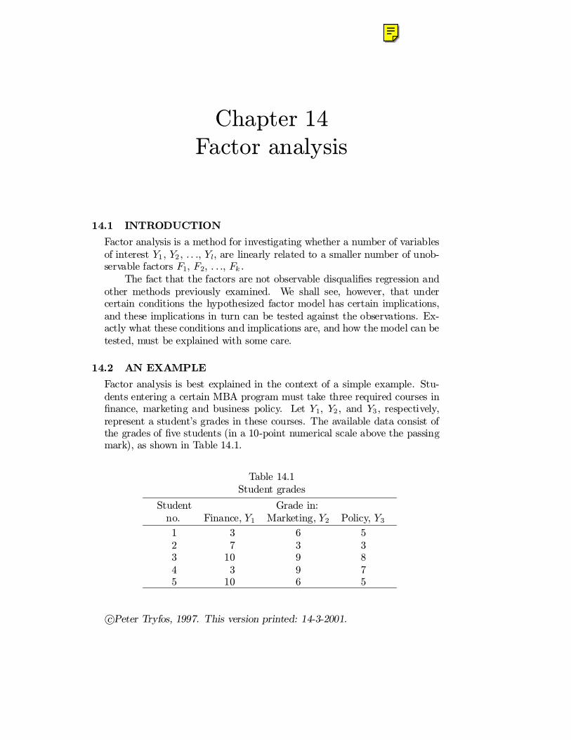
Factor analysis is best explained in the context of a simple example. Stu-dents entering a certain MBA program must take three required courses in¯nance, marketing and business policy. Let Y1, Y2 , and Y3 , respectively,represent a student's grades in these courses. The available data consist ofthe grades of ¯ve students (in a 10-point numerical scale above the passingmark), as shown in Table 14.1.
Table 14.1Student grades
Student Grade in:no. Finance, Y1 Marketing, Y2 Policy, Y3
1 3 6 52 7 3 33 10 9 84 3 9 75 10 6 5
c°Peter Tryfos, 1997. This version printed: 14-3-2001.
2 Chapter 14: Factor analysis
It has been suggested that these grades are functions of two underlyingfactors, F1 and F2, tentatively and rather loosely described as quantitativeability and verbal ability, respectively. It is assumed that each Y variable islinearly related to the two factors, as follows:
Y1 = ¯10 +¯11F1 +¯12F2 + e1
Y2 = ¯20 +¯21F1 +¯22F2 + e2
Y3 = ¯30 +¯31F1 +¯32F2 + e3
(14:1)
The error terms e1, e2, and e3 , serve to indicate that the hypothesizedrelationships are not exact.
In the special vocabulary of factor analysis, the parameters ¯ij arereferred to as loadings. For example, ¯12 is called the loading of variable Y1
on factor F2.In this MBA program, ¯nance is highly quantitative, while marketing
and policy have a strong qualitative orientation. Quantitative skills shouldhelp a student in ¯nance, but not in marketing or policy. Verbal skills shouldbe helpful in marketing or policy but not in ¯nance. In other words, it isexpected that the loadings have roughly the following structure:
Loading on:Variable, Yi F1 , ¯i1 F2, ¯i2
Y1 + 0Y2 0 +Y3 0 +
The grade in the ¯nance course is expected to be positively related toquantitative ability but unrelated to verbal ability; the grades in marketingand policy, on the other hand, are expected to be positively related to verbalability but unrelated to quantitative ability. Of course, the zeros in thepreceding table are not expected to be exactly equal to zero. By `0' wemean approximately equal to zero and by `+' a positive number substantiallydi®erent from zero.
It may appear that the loadings can be estimated and the expectationstested by regressing each Y against the two factors. Such an approach,however, is not feasible because the factors cannot be observed. An entirelynew strategy is required.
Let us turn to the process that generates the observations on Y1, Y2 andY3 according to (14.1). The simplest model of factor analysis is based ontwo assumptions concerning the relationships (14.1). We shall ¯rst describethese assumptions and then examine their implications.
A1: The error terms ei are independent of one another, and suchthat E(ei) = 0 and Var(ei) = ¾2
i .

14.2 An example 3
One can think of each ei as the outcome of a random draw with replace-ment from a population of ei-values having mean 0 and a certain variance¾2i . A similar assumption was made in regression analysis (Section 3.2).
A2: The unobservable factors Fj are independent of one anotherand of the error terms, and are such thatE(Fj) = 0 and V ar(Fj) =1.
In the context of the present example, this means in part that there isno relationship between quantitative and verbal ability. In more advancedmodels of factor analysis, the condition that the factors are independentof one another can be relaxed. As for the factor means and variances, theassumption is that the factors are standardized. It is an assumption madefor mathematical convenience; since the factors are not observable, we mightas well think of them as measured in standardized form.
Let us now examine some implications of these assumptions. Eachobservable variable is a linear function of independent factors and errorterms, and can be written as
Yi = ¯i0 + ¯i1F1 +¯i2F2 + (1)ei:
The variance of Yi can be calculated by applying the result in AppendixA.11:
V ar(Yi) = ¯2i1V ar(F1) + ¯2
i2Var(F2)+ (1)2V ar(ei)
= ¯2i1 +¯2
i2 + ¾2i :
We see that the variance of Yi consists of two parts:
Var(Yi) = ¯2i1 +¯2
i2| {z }communality
+ ¾2i|{z}
speci¯c variance
:
The ¯rst, the communality of the variable, is the part that is explained bythe common factors F1 and F2 . The second, the speci¯c variance, is thepart of the variance of Yi that is not accounted by the common factors. Ifthe two factors were perfect predictors of grades, then e1 = e2 = e3 = 0always, and ¾2
1 = ¾22 = ¾2
3 = 0:To calculate the covariance of any two observable variables, Yi and Yj ,
we can write
Yi = ¯i0 +¯i1F1 + ¯i2F2 +(1)ei +(0)ej ; and
Yj = ¯j0 +¯j1F1 +¯j2F2 +(0)ei +(1)ej ;
and apply the result in Appendix A.12 to ¯nd
4 Chapter 14: Factor analysis
Cov(Yi; Yj) = ¯i1¯j1Var(F1)+ ¯i2¯j2V ar(F2) + (1)(0)Var(ei)
+ (0)(1)V ar(ej)
= ¯i1¯j1 +¯i2¯j2:
We can arrange all the variances and covariances in the form of thefollowing table:
Variable:Variable: Y1 Y2 Y3
Y1 ¯211 +¯2
12 + ¾21 ¯21¯11 + ¯22¯12 ¯31¯11 +¯32¯12
Y2 ¯11¯21 + ¯12¯22 ¯221 +¯2
22 + ¾22 ¯21¯31 +¯22¯32
Y3 ¯11¯31 + ¯12¯32 ¯21¯31 + ¯22¯32 ¯231 + ¯2
32 + ¾23
We have placed the variances of the Y variables in the diagonal cells ofthe table and the covariances o® the diagonal. These are the variances andcovariances implied by the model's assumptions. We shall call this table thetheoretical variance covariance matrix (see Appendix A.11). The matrix issymmetric, in the sense that the entry in row 1 and column 2 is the sameas that in row 2 and column 1, and so on.
Let us now turn to the available data. Given observations on the vari-ables Y1 , Y2 , and Y3 , we can calculate the observed variances and covariancesof the variables, and arrange them in the observed variance covariance ma-trix:
Variable:Variable: Y1 Y2 Y3
Y1 S21 S12 S13
Y2 S21 S22 S23
Y3 S31 S32 S23
Thus, S21 is the observed variance of Y1, S12 the observed covariance
of Y1 and Y2 , and so on. It is understood, of course, the S12 = S21, S13 =S31 , and so on; the matrix, in other words, is symmetric. It can be easilycon¯rmed that the observed variance covariance matrix for the data of Table14.1 is as follows: 0
@9:84 ¡0:36 0:44
¡0:36 5:04 3:840:44 3:84 3:04
1A

14.3 Factor loadings are not unique 5
On the one hand, therefore, we have the observed variances and covari-ances of the variables; on the other, the variances and covariances impliedby the factor model. If the model's assumptions are true, we should be ableto estimate the loadings ¯ij so that the resulting estimates of the theoreticalvariances and covariances are close to the observed ones. We shall soon seehow these estimates can be obtained, but ¯rst let us examine an importantfeature of the factor model.
14.3 FACTOR LOADINGS ARE NOT UNIQUE
We would like to demonstrate that the loadings are not unique, that is,that there exist an in¯nite number of sets of values of the ¯ij yielding thesame theoretical variances and covariances. Consider ¯rst an arbitrary setof loadings de¯ning what we shall call Model A:
Y1 = 0:5 F1 +0:5 F2 + e1
Y2 = 0:3 F1 +0:3 F2 + e2
Y3 = 0:5 F1 ¡ 0:5 F2 + e3
It is not di±cult to verify that the theoretical variance covariancematrixis 0
@0:5 + ¾2
1 0:3 00:3 0:18 +¾2
2 00 0 0:5 +¾2
3
1A
For example, V ar(Y1) = (0:5)2 + (0:5)2 + ¾21 = 0:5 + ¾2
1 ; Cov(Y1 ;Y2) =(0:5)(0:3) + (0:5)(0:3) = 0:3; and so on.
Next, consider Model B, having a di®erent set of ¯ij :
Y1 = (p
2=2) F1 +0 F2 + e1
Y2 = (0:3p
2) F1 +0 F2 + e2
Y3 = 0 F1 ¡ (p
2=2) F2 + e3
It can again be easily con¯rmed that the theoretical variances and covari-ances are identical to those of Model A. For example, V ar(Y1) = (
p2=2)2 +
(0)2 + ¾21 = 0:5 + ¾2
1 ; Cov(Y1; Y2) = (p
2=2)(0:3p
2) + (0)(0) = 0:3; and soon.
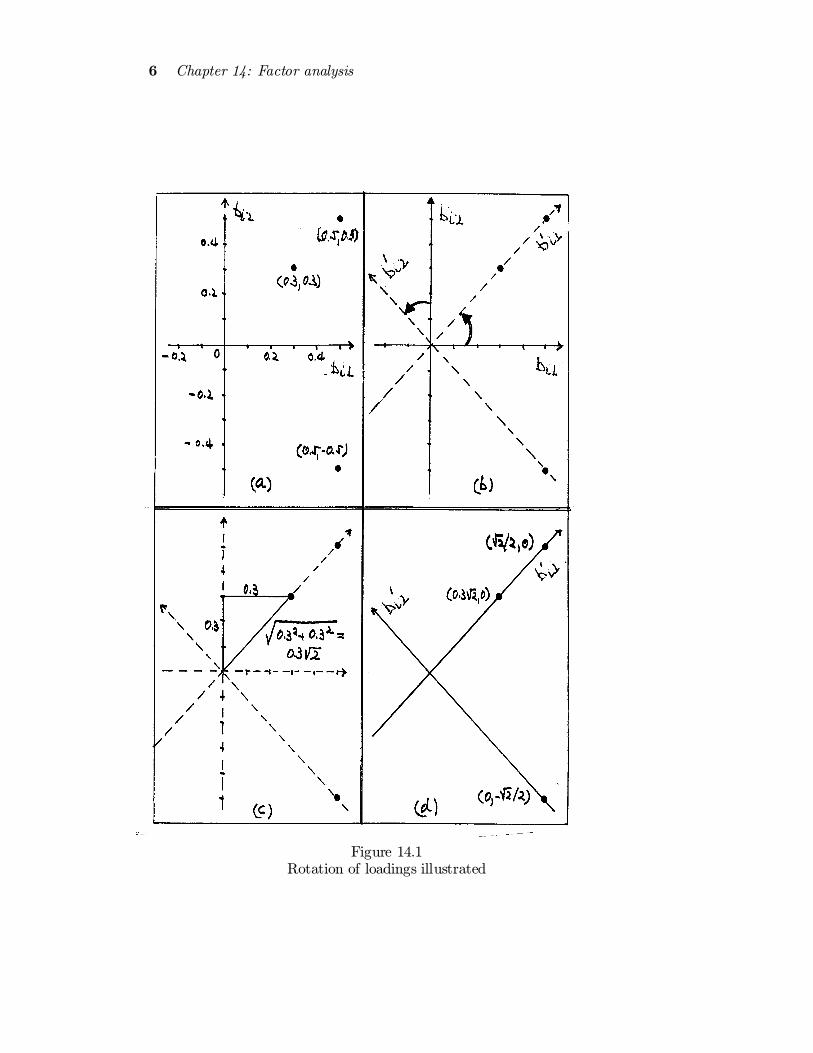
Examine now panel (a) of Figure 14.1. Along the horizontal axis weplot the coe±cient of F1, and along the vertical axis the coe±cient of F2
for each equation of Model A. The coe±cients of F1 and F2 in the ¯rstequation are plotted as the point with coordinates (0.5, 0.5); those of thesecond equation as the point (0.3, 0.3), and those of the third as the point(0.5, ¡0:5).
6 Chapter 14: Factor analysis
Figure 14.1Rotation of loadings illustrated
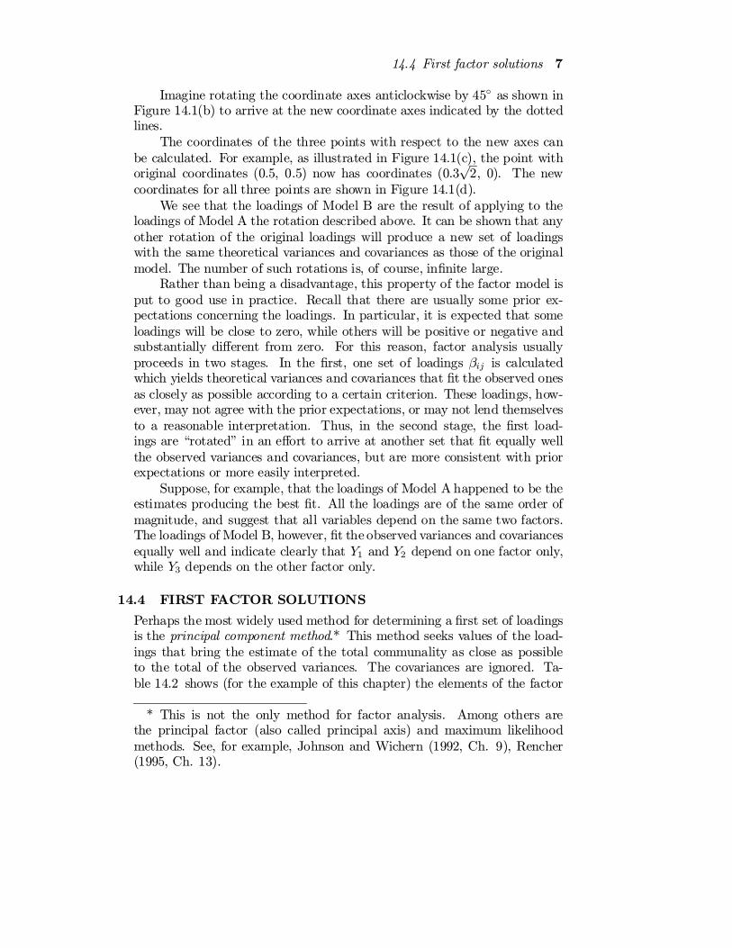
14.4 First factor solutions 7
Imagine rotating the coordinate axes anticlockwise by 45± as shown inFigure 14.1(b) to arrive at the new coordinate axes indicated by the dottedlines.
The coordinates of the three points with respect to the new axes canbe calculated. For example, as illustrated in Figure 14.1(c), the point withoriginal coordinates (0.5, 0.5) now has coordinates (0:3
p2, 0). The new
coordinates for all three points are shown in Figure 14.1(d).We see that the loadings of Model B are the result of applying to the
loadings of Model A the rotation described above. It can be shown that anyother rotation of the original loadings will produce a new set of loadingswith the same theoretical variances and covariances as those of the originalmodel. The number of such rotations is, of course, in¯nite large.
Rather than being a disadvantage, this property of the factor model isput to good use in practice. Recall that there are usually some prior ex-pectations concerning the loadings. In particular, it is expected that someloadings will be close to zero, while others will be positive or negative andsubstantially di®erent from zero. For this reason, factor analysis usuallyproceeds in two stages. In the ¯rst, one set of loadings ¯ij is calculatedwhich yields theoretical variances and covariances that ¯t the observed onesas closely as possible according to a certain criterion. These loadings, how-ever, may not agree with the prior expectations, or may not lend themselvesto a reasonable interpretation. Thus, in the second stage, the ¯rst load-ings are \rotated" in an e®ort to arrive at another set that ¯t equally wellthe observed variances and covariances, but are more consistent with priorexpectations or more easily interpreted.
Suppose, for example, that the loadings of Model A happened to be theestimates producing the best ¯t. All the loadings are of the same order ofmagnitude, and suggest that all variables depend on the same two factors.The loadings of Model B, however, ¯t the observed variances and covariancesequally well and indicate clearly that Y1 and Y2 depend on one factor only,while Y3 depends on the other factor only.
14.4 FIRST FACTOR SOLUTIONS
Perhaps the most widely used method for determining a ¯rst set of loadingsis the principal component method.* This method seeks values of the load-ings that bring the estimate of the total communality as close as possibleto the total of the observed variances. The covariances are ignored. Ta-ble 14.2 shows (for the example of this chapter) the elements of the factor
* This is not the only method for factor analysis. Among others arethe principal factor (also called principal axis) and maximum likelihoodmethods. See, for example, Johnson and Wichern (1992, Ch. 9), Rencher(1995, Ch. 13).
8 Chapter 14: Factor analysis
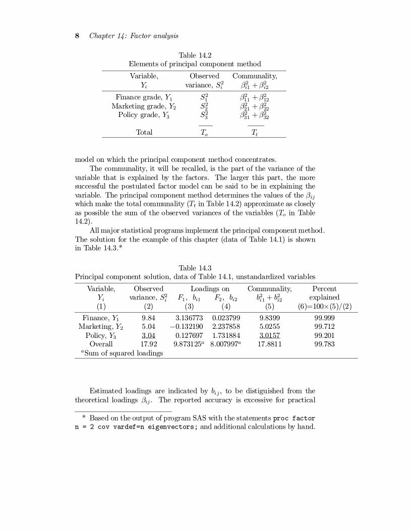
Table 14.2Elements of principal component method
Variable, Observed Communality,Yi variance, S2
i ¯2i1 +¯2
i2
Finance grade, Y1 S21 ¯2
11 +¯212
Marketing grade, Y2 S22 ¯2
21 +¯222
Policy grade, Y3 S23 ¯2
31 +¯232
Total To Tt
model on which the principal component method concentrates.The communality, it will be recalled, is the part of the variance of the
variable that is explained by the factors. The larger this part, the moresuccessful the postulated factor model can be said to be in explaining thevariable. The principal component method determines the values of the ¯ijwhich make the total communality (Tt in Table 14.2) approximate as closelyas possible the sum of the observed variances of the variables (To in Table14.2).
All major statistical programs implement the principal componentmethod.The solution for the example of this chapter (data of Table 14.1) is shownin Table 14.3.*
Table 14.3Principal component solution, data of Table 14.1, unstandardized variables
Variable, Observed Loadings on Communality, PercentYi variance, S2
i F1 ; bi1 F2 ; bi2 b2i1 + b2i2 explained(1) (2) (3) (4) (5) (6)=100£(5)/(2)
Finance, Y1 9.84 3.136773 0.023799 9.8399 99.999Marketing, Y2 5.04 ¡0.132190 2.237858 5.0255 99.712
Policy, Y3 3.04 0.127697 1.731884 3.0157 99.201Overall 17.92 9.873125a 8.007997a 17.8811 99.783
aSum of squared loadings
Estimated loadings are indicated by bij , to be distiguished from thetheoretical loadings ¯ij . The reported accuracy is excessive for practical
* Based on the output of program SAS with the statements proc factor
n = 2 cov vardef=n eigenvectors; and additional calculations by hand.
14.4 First factor solutions 9
purposes (two or three decimal places would have been su±cient); it isintended to assist comparisons with the output of other computer programs.
We see that the solution supports the expectations. The loadings onF1 are relatively large for Y1 but close to zero for Y2 and Y3; the loadings onF2 are close to zero for Y1 but relatively high for Y2 and Y3 . Thus, F1 couldbe interpreted as quantitative, and F2 as verbal, ability. We also observethat the factor model explains nearly 100%, 99.7%, and 99.2% respectivelyof the observed variance of ¯nance, marketing and policy grades. Overall,the two factors explain 99.78% of the sum of all observed variances.
The sum of squared loadings on F1 ,P
i b2i1 , can be interpreted as the
contribution of F1 , and that on F2,P
i b2i2, as the contribution of F2 in
explaining the sum of the observed variances. In Table 14.3,
X
i
b2i1 = (3:136773)2 + ¢ ¢ ¢+ (0:127697)2 = 9:873125;
and X
i
b2i2 = (0:023799)2 + ¢ ¢ ¢+ (1:731884)2 = 8:007997:
Thus, F1 explains about 9.873/19.92 or 55.1%, and F2 about 44.7% of thesum of the observed variances.
The estimate of the speci¯c variance of Yi, ¾2i , is the di®erence between the
observed variance and estimated communality of Yi:
Variable, Observed Estimated EstimatedYi variance communality spec. variance
Finance, Y1 9.84 9.8399 0.0001Marketing, Y2 5.04 5.0255 0.0145
Policy, Y3 3.04 3.0157 0.0243
Having the total communality approximate as closely as possible thesum of the observed variances (in e®ect, attaching the same weight to eachvariable) makes sense when the Y variables are measured in the same units,as in the example of this chapter. When this is not so, however, it is clearthat the principal component method will favor the variables with largevariances at the expense of those with small ones.
For this reason, it is customary to standardize the variables prior tosubjecting them to the principal component method so that all have meanzero and variance equal to one. This is accomplished by subtracting fromeach observation (Yij) the mean of the variable (¹Yi) and dividing the resultby the standard deviation (Si) of the variable to obtain the standardizedobservation Y 0ij ,
Y 0ij =Yij ¡ ¹YiSi
:
10 Chapter 14: Factor analysis
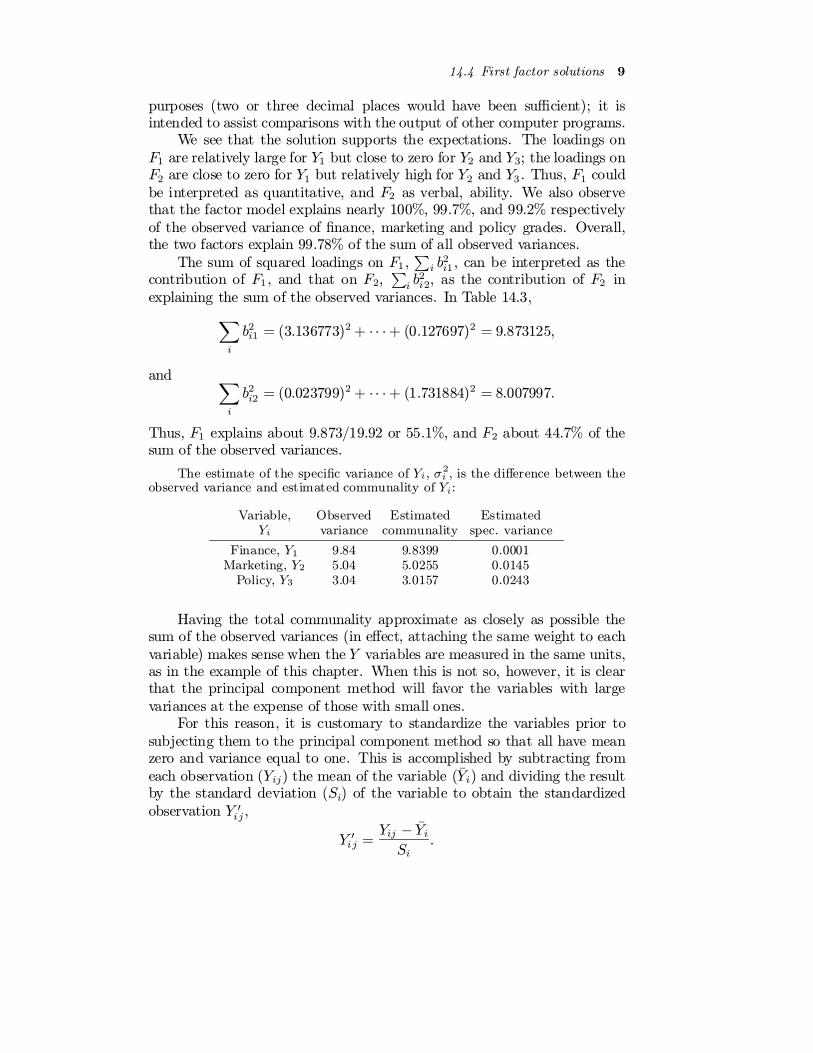
It can be shown that the covariances of the standardized variables are equalto the correlation coe±cients of the original variables (the variances of thestandardized variables are, of course, equal to 1).
This last result can be easily veri¯ed using the data of Table 14.1. First, wecalculate
Y1 Y2 Y3
Mean, ¹Yi: 6.6 6.6 5.6Variance, S2
i : 9.84 5.04 3.04Std. Dev., Si: 3.1369 2.2450 1.7436
The observations of the standardized variables are shown in the following table:
Y 01 Y 02 Y 03
¡1.14763 ¡0.26726 ¡0.344120.12751 ¡1.60356 ¡1.491171.08387 1.06904 1.37646
¡1.14763 1.06904 0.802941.08387 ¡0.26726 ¡0.34412
For example, the ¯rst standardized variable is given by
Y 01j =Y1j ¡ 6:6
3:1369:
It can be con¯rmed that the means of the standardized variables are equal to 0,and their variances and standard deviations equal to 1.
The covariance of Y1 and Y2 is
S12 =1
n
XY1Y2 ¡ ¹Y1 ¹Y2 = (216)¡ (6:6)(6:6) = ¡0:36:
The correlation coe±cient of Y1 and Y2 is
r12 =S12
S1S2=
¡0:36
(3:1369)(2:245)= ¡0:0511;
and is equal to the covariance of Y 01 and Y 02 ,
S012 =1
n
XY 01Y
02 ¡ ¹Y 01 ¹Y 02 = (¡0:2556) ¡ (0)(0) = ¡0:0511:
In general, Cov(Y 0i ; Y0j ) = Cor(Yi; Yj). The correlation matrix of the original
variables (equal to the covariance matrix of the standardized variables) is
Ã1 ¡0:0511 0:0804
¡0:0511 1 0:98100:0804 0:9810 1
!
The reader is asked to con¯rm the remaining numbers in Problem 14.3.
14.4 First factor solutions 11
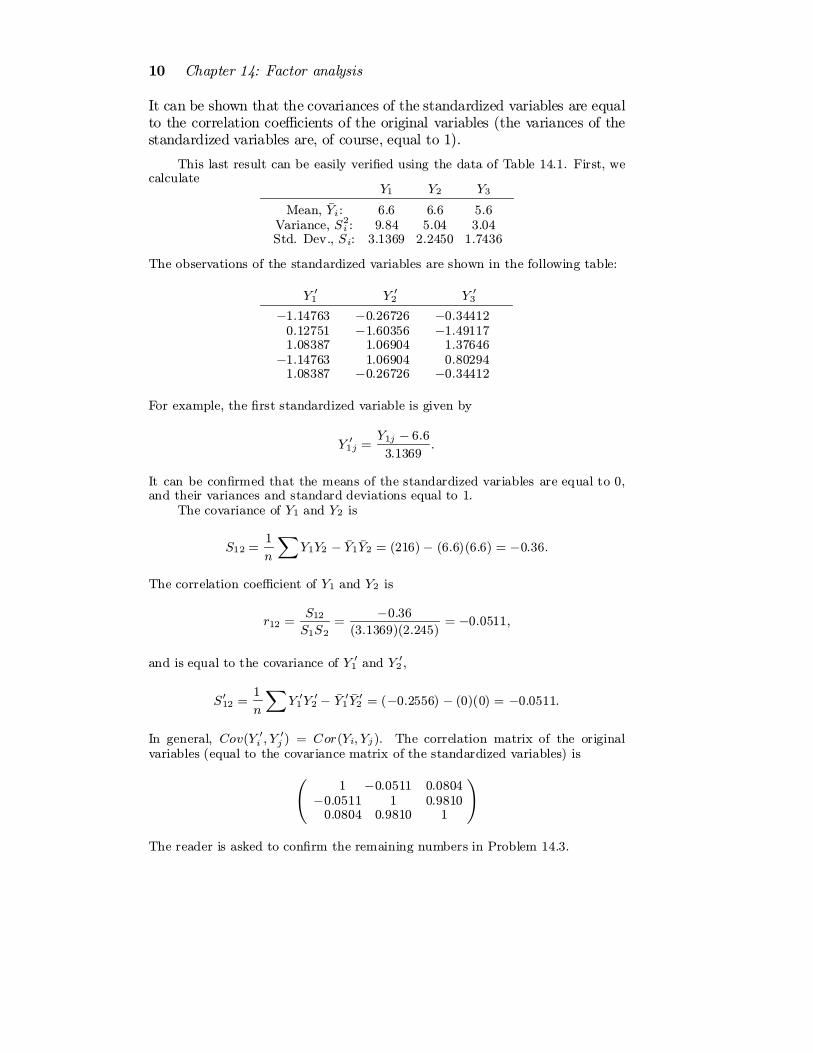
Standardization, in e®ect, subjects the observed correlation matrix ofthe original variables|rather than the observed variance covariance matrix|to the principal component method. The principal component solution forstandardized variables will not necessarily be the same as that for unstan-dardized ones.
In some statistical programs (e.g., SPSS, SAS), standardization andthe principal component method are the default options. Figure 14.2 showsthe default output of proc factor of program SAS for the example of thischapter and the data in Table 14.1.*
The computer output is translated and interpreted in Table 14.4.
Table 14.4Principal component solution, data of Table 14.1, standardized variables
Standardized Observed Loadings on Communality, Percentvariable, Y 0i variance, S02i F1 ; bi1 F2; bi2 b2i1 + b2i2 explained
(1) (2) (3) (4) (5) (6)=100£(5)/(2)
Finance, Y 01 1 0.02987 0.99951 0.99991 99.991Marketing, Y 02 1 0.99413 ¡0.08153 0.99494 99.494
Policy, Y 03 1 0.99613 0.05139 0.99492 99.492Overall 3 1.981463a 1.008306a 2.98977 99.659
aSum of squared loadings
As with the original unstandardized variables, marketing and policygrades depend on one common factor (which can be interpreted as ver-bal ability) but not appreciably on the other (quantitative ability); the re-verse holds for ¯nance grades. Unlike the unstandardized case, however,verbal ability contributes more than quantitative ability: F1 accounts for1.981463/3 or about 66%, while F2 accounts for 1.008306/3 or about 33.6%of the sum of the observed variances. This is why the verbal ability factoris listed ¯rst in the computer output and Table 14.4 (the labels F1 and F2
are, of course, arbitrary). The two factors together explain 2.98977/3 or99.659% of the sum of the observed variances of the standardized variables,slightly less than with the original variables.
* Readers familiar with linear algebra may want to know that the princi-pal component solution involves the eigenvalues (characteristic values) andeigenvectors (characteristic vectors) of the observed variance covariance orcorrelation matrix. Hence the appearance of these terms in the output ofcomputer programs. For a clear mathematical exposition of the principalcomponent method see, for example, Johnson and Wichern, ibid.

12 Chapter 14: Factor analysis
Figure 14.2SAS output, data of Table 14.1
14.5 FACTOR ROTATION
When the ¯rst factor solution does not reveal the hypothesized structure ofthe loadings, it is customary to apply rotation in an e®ort to ¯nd anotherset of loadings that ¯t the observations equally well but can be more easilyinterpreted. As it is impossible to examine all such rotations, computerprograms carry out rotations satisfying certain criteria.
Perhaps the most widely used of these is the varimax criterion. It seeksthe rotated loadings that maximize the variance of the squared loadings foreach factor; the goal is to make some of these loadings as large as possible,

14.5 Factor rotation 13
and the rest as small as possible in absolute value. The varimax methodencourages the detection of factors each of which is related to few variables.It discourages the detection of factors in°uencing all variables.
The quartimax criterion, on the other hand, seeks to maximize thevariance of the squared loadings for each variable, and tends to producefactors with high loadings for all variables.
Figure 14.3SAS output continued, data of Table 14.1
Figure 14.3 shows the output produced by the SAS program, instructedto apply the varimax rotation to the ¯rst set of loadings shown in Figure14.3.
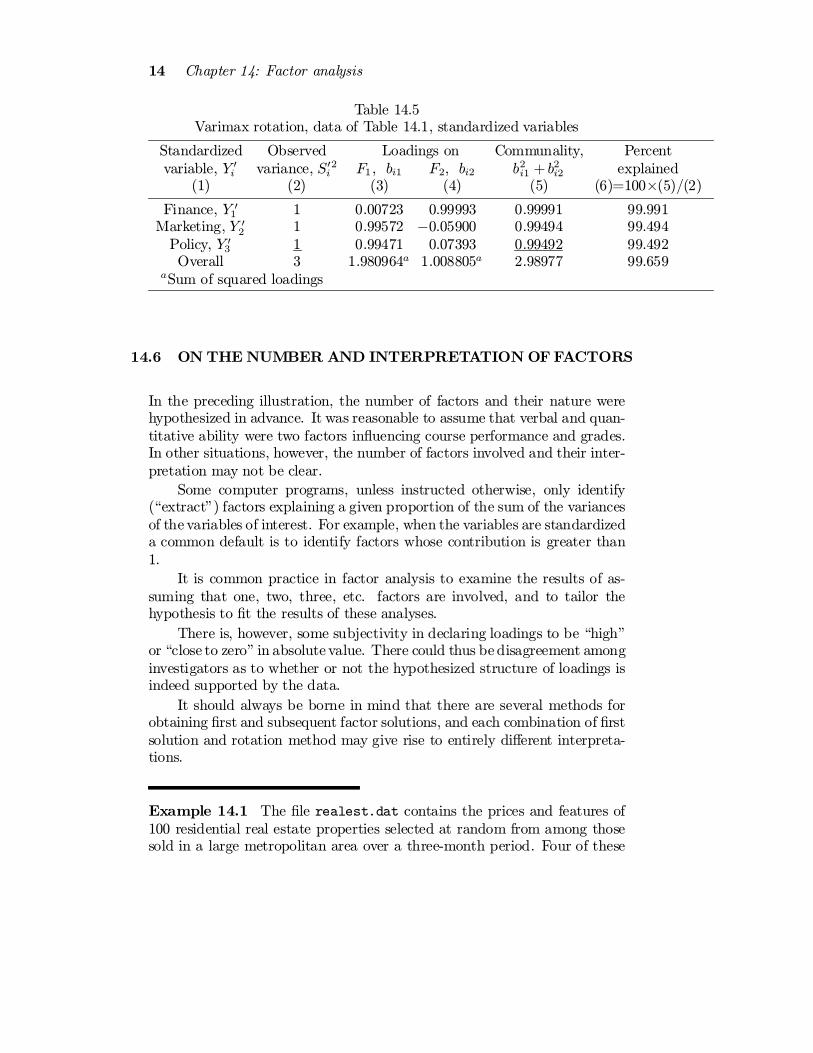
This output is translated and interpreted in Table 14.5.The estimates of the communality of each variable and of the total
communality are the same as in Table 14.4, but the contributions of eachfactor di®er slightly. In this example, rotation did not alter appreciably the¯rst estimates of the loadings or the proportions of the sum of the observedvariances explained by the two factors.
14 Chapter 14: Factor analysis
Table 14.5Varimax rotation, data of Table 14.1, standardized variables
Standardized Observed Loadings on Communality, Percentvariable, Y 0i variance, S02i F1 ; bi1 F2; bi2 b2i1 + b2i2 explained
(1) (2) (3) (4) (5) (6)=100£(5)/(2)
Finance, Y 01 1 0.00723 0.99993 0.99991 99.991Marketing, Y 02 1 0.99572 ¡0.05900 0.99494 99.494
Policy, Y 03 1 0.99471 0.07393 0.99492 99.492Overall 3 1.980964a 1.008805a 2.98977 99.659
aSum of squared loadings
14.6 ON THE NUMBER AND INTERPRETATION OF FACTORS
In the preceding illustration, the number of factors and their nature werehypothesized in advance. It was reasonable to assume that verbal and quan-titative ability were two factors in°uencing course performance and grades.In other situations, however, the number of factors involved and their inter-pretation may not be clear.
Some computer programs, unless instructed otherwise, only identify(\extract") factors explaining a given proportion of the sum of the variancesof the variables of interest. For example, when the variables are standardizeda common default is to identify factors whose contribution is greater than1.
It is common practice in factor analysis to examine the results of as-suming that one, two, three, etc. factors are involved, and to tailor thehypothesis to ¯t the results of these analyses.
There is, however, some subjectivity in declaring loadings to be \high"or \close to zero" in absolute value. There could thus be disagreement amonginvestigators as to whether or not the hypothesized structure of loadings isindeed supported by the data.
It should always be borne in mind that there are several methods forobtaining ¯rst and subsequent factor solutions, and each combination of ¯rstsolution and rotation method may give rise to entirely di®erent interpreta-tions.
Example 14.1 The ¯le realest.dat contains the prices and features of100 residential real estate properties selected at random from among thosesold in a large metropolitan area over a three-month period. Four of these
14.6 On the number and interpretation of factors 15
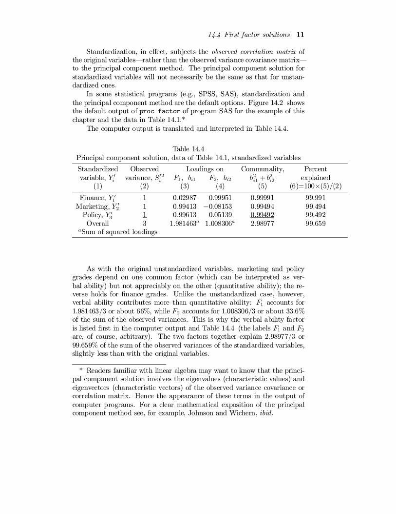
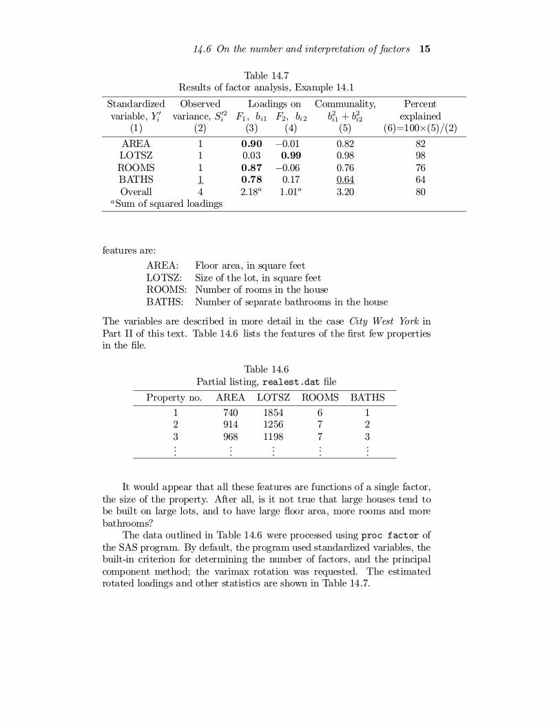
Table 14.7Results of factor analysis, Example 14.1
Standardized Observed Loadings on Communality, Percentvariable, Y 0i variance, S02i F1 ; bi1 F2; bi2 b2i1 + b2i2 explained
(1) (2) (3) (4) (5) (6)=100£(5)/(2)
AREA 1 0.90 ¡0.01 0.82 82LOTSZ 1 0.03 0.99 0.98 98ROOMS 1 0.87 ¡0.06 0.76 76BATHS 1 0.78 0.17 0.64 64Overall 4 2.18a 1.01a 3.20 80
aSum of squared loadings
features are:
AREA: Floor area, in square feetLOTSZ: Size of the lot, in square feetROOMS: Number of rooms in the houseBATHS: Number of separate bathrooms in the house
The variables are described in more detail in the case City West York inPart II of this text. Table 14.6 lists the features of the ¯rst few propertiesin the ¯le.
Table 14.6Partial listing, realest.dat ¯le
Property no. AREA LOTSZ ROOMS BATHS
1 740 1854 6 12 914 1256 7 23 968 1198 7 3...
......
......
It would appear that all these features are functions of a single factor,the size of the property. After all, is it not true that large houses tend tobe built on large lots, and to have large °oor area, more rooms and morebathrooms?
The data outlined in Table 14.6 were processed using proc factor ofthe SAS program. By default, the program used standardized variables, thebuilt-in criterion for determining the number of factors, and the principalcomponent method; the varimax rotation was requested. The estimatedrotated loadings and other statistics are shown in Table 14.7.
16 Chapter 14: Factor analysis
Contrary to prior expectations, two factors|not one|were identi¯edby the program. The ¯rst factor has high loadings for AREA, ROOMS, andBATHS; it can be interpreted as the size of the house. The second factorhas high loadings only for LOTSZ, and can be interpreted as the size of thelot. In the metropolitan area from which the data were selected, therefore,the size of the lot can be assumed to be unrelated to the size of the houseproper. The size of the house explains 2.18/4 or 54.5%, and the size ofthe lot 1.01/4 or 25.45% of the sum of the variances of the standardizedvariables. The two factors together account for 80% of the total variance.
14.7 TO SUM UP
² Factor analysis is a method for investigating whether a number ofvariables of interest are linearly related to a smaller number of unobservablefactors.
² In the special vocabulary of factor analysis, the parameters of theselinear functions are referred to as loadings.
² Under certain conditions (A1 and A2 in the text), the theoreticalvariance of each variable and the covariance of each pair of variables can beexpressed in terms of the loadings and the variance of the error terms.
² The communality of a variable is the part of its variance that isexplained by the common factors. The speci¯c variance is the part of thevariance of the variable that is not accounted by the common factors.
² There exist an in¯nite number of sets of loadings yielding the sametheoretical variances and covariances.
² Factor analysis usually proceeds in two stages. In the ¯rst, one set ofloadings is calculated which yields theoretical variances and covariances that¯t the observed ones as closely as possible according to a certain criterion.These loadings, however, may not agree with the prior expectations, or maynot lend themselves to a reasonable interpretation. Thus, in the secondstage, the ¯rst loadings are \rotated" in an e®ort to arrive at another setof loadings that ¯t equally well the observed variances and covariances, butare more consistent with prior expectations or more easily interpreted.
² A method widely used for determining a ¯rst set of loadings is theprincipal component method. This method seeks values of the loadings thatbring the estimate of the total communality as close as possible to the totalof the observed variances.
²When the variables are notmeasured in the sameunits, it is customaryto standardize them prior to subjecting them to the principal componentmethod so that all have mean equal to zero and variance equal to one.
² The varimax rotation method encourages the detection of factors eachof which is related to few variables. It discourages the detection of factorsin°uencing all variables.
Problems 17
² There is considerable subjectivity in determining the number of fac-tors and the interpretation of these factors. There are several methods forobtaining ¯rst and rotated factor solutions, and each such solution may giverise to a di®erent interpretation.
PROBLEMS
14.1 Con¯rm the results presented in Tables 14.4 and 14.5 using the data ofTable 14.1 and a statistical program for factor analysis.
14.2 Con¯rm the results given in Table 14.7 using the data in the ¯le realest.datand a statistical program for factor analysis.
14.3 Using the data of Table 14.1 and in the manner of Section 14.4, con¯rmthat the covariances of the standardized variables Y 01, Y
02 , and Y 03 , are equal to the
correlation coe±cients of the original variables Y1, Y2, and Y3 .
14.4 Two observable variables, Y1 and Y2, are thought to be linearly related toa common unobservable factor F :
Y1 = ¯10 + ¯11F + e1
Y2 = ¯20 + ¯21F + e2
Assume that F , e1, and e2 satisfy conditions A1 and A2 of Section 14.2.(a) Derive the variances and covariance of Y1 and Y2. Arrange them in the
form of a theoretical variance covariance matrix.(b) Write the form of the observed variance covariance matrix.(c) Suppose there are four observations on variables Y1 and Y2:
Y1 Y2
10 -5-4 20 16 -3
Calculate the observed variance covariance matrix.(d) Estimate the loadings ¯ij according to the principal component method
with the help of a statistical program.(e) Is it possible to rotate the loadings in this case? Explain.
14.5 Refer to Model A of Section 14.3. Rotate the loadings by 90o in an anti-clockwise direction. Show that the variance covariance matrix of the variables isthe same after rotation. What is the meaning of the rotation in this case?
14.6 Three observable variables are known to be related to two unobservablefactors as follows:
Y1 = ¡0:7F1 + 0:6F2 + e1
Y2 = 0:5F1 + 0:4F2 + e2
Y3 = 0:2F1 ¡ 0:3F2 + e3
(a) In the manner of Section 14.3, rotate the loadings by 45o in a clockwisedirection.
(b) Con¯rm that the variance covariance matrix of the variables is the samebefore and after rotation.
18 Chapter 14: Factor analysis
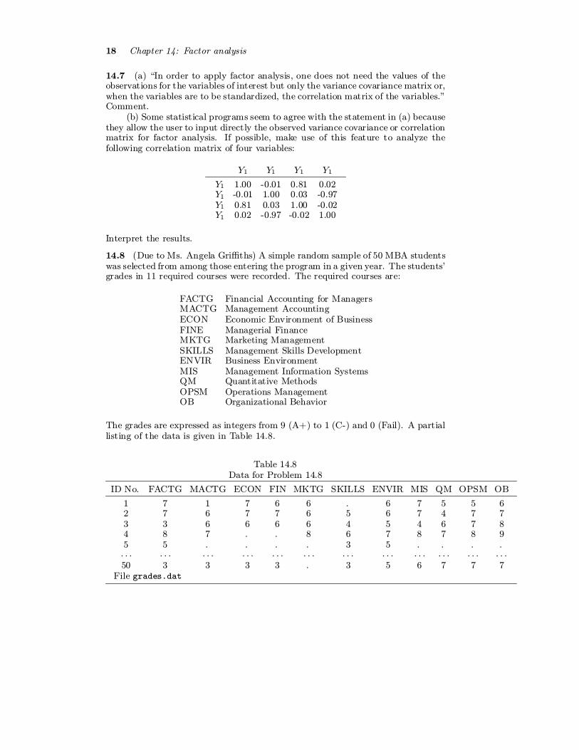
14.7 (a) \In order to apply factor analysis, one does not need the values of theobservations for the variables of interest but only the variance covariance matrix or,when the variables are to be standardized, the correlation matrix of the variables."Comment.
(b) Some statistical programs seem to agree with the statement in (a) becausethey allow the user to input directly the observed variance covariance or correlationmatrix for factor analysis. If possible, make use of this feature to analyze thefollowing correlation matrix of four variables:
Y1 Y1 Y1 Y1
Y1 1.00 -0.01 0.81 0.02Y1 -0.01 1.00 0.03 -0.97Y1 0.81 0.03 1.00 -0.02Y1 0.02 -0.97 -0.02 1.00
Interpret the results.
14.8 (Due to Ms. Angela Gri±ths) A simple random sample of 50 MBA studentswas selected from among those entering the program in a given year. The students'grades in 11 required courses were recorded. The required courses are:
FACTG Financial Accounting for ManagersMACTG Management AccountingECON Economic Environment of BusinessFINE Managerial FinanceMKTG Marketing ManagementSKILLS Management Skills DevelopmentENVIR Business EnvironmentMIS Management Information SystemsQM Quantitative MethodsOPSM Operations ManagementOB Organizational Behavior
The grades are expressed as integers from 9 (A+) to 1 (C-) and 0 (Fail). A partiallisting of the data is given in Table 14.8.
Table 14.8Data for Problem 14.8
ID No. FACTG MACTG ECON FIN MKTG SKILLS ENVIR MIS QM OPSM OB
1 7 1 7 6 6 . 6 7 5 5 62 7 6 7 7 6 5 6 7 4 7 73 3 6 6 6 6 4 5 4 6 7 84 8 7 . . 8 6 7 8 7 8 95 5 . . . . 3 5 . . . .¢ ¢ ¢ ¢ ¢ ¢ ¢ ¢ ¢ ¢ ¢ ¢ ¢ ¢ ¢ ¢ ¢ ¢ ¢ ¢ ¢ ¢ ¢ ¢ ¢ ¢ ¢ ¢ ¢ ¢ ¢ ¢ ¢ ¢ ¢ ¢50 3 3 3 3 . 3 5 6 7 7 7
File grades.dat

Problems 19
Figure 14.4Factor analysis results, Problem 14.8(a)
Many students had not completed all required courses; missing grades areindicated by a period.
(a) Figure 14.4 shows the output of a computer program for factor analysisdirected to extract only one factor (program SAS with the statement proc factorn=1). Interpret and comment on the results.
(b) Can the analysis be improved? If so, carry out your suggestions using the¯le grades.dat and a program for factor analysis.
14.9 The ¯le bridge.dat is described in Problem 4.12 and includes the followingfeatures of 45 bridges constructed by the Department of Transportation:
TIME: Design time, in man-daysDAREA: Deck area of bridge (000 sq.ft.)CCOST: Construction cost ($0000)DWGS: Number of structural drawings
LENGTH: Length of bridge, in feetSPANS: Number of spansDDIFF: Degree of di±culty of bridge design (=0 easy, =1 complex)

20 Chapter 14: Factor analysis
A statistical program for factor analysis routinely processed the data ac-cording to its built-in defaults (standardization, principal component estimation,varimax rotation). It extracted two factors and produced the loadings shown inTable 14.9.
Table 14.9Rotated factor loadings,
Problem 14.9
Variable Factor 1 Factor 2
TIME 0.69732 0.47572DAREA 0.74797 0.44545CCOST 0.83123 0.35001DWGS 0.59594 0.64808
LENGTH 0.93742 0.16039SPANS 0.86564 0.20127DDIFF 0.16549 0.93573
(a) Calculate the communality of each variable and the percentage of itsvariance that is explained by the factors. Calculate the percentage of the totalvariance that is explained by each factor and by both factors jointly.
(b) Interpret the results of factor analysis.(c) Con¯rm the results using the data in the ¯le bridge.dat and a program
for factor analysis.(d) Of what possible use is this type of analysis? Can it be improved? If
so, carry out your recommendations using the data in the ¯le bridge.dat and aprogram for factor analysis.
14.10 The ¯le mpg.dat is described in Problem 5.15 and includes the followingfeatures of 116 car models:
ED: Engine displacement (litres)CYL: Number of cylinders
HP: Horsepower (bhp)WEIGHT: Weight (lbs.)
MPG: Fuel mileage (miles per gallon)
The data on these variables were processed by a program for factor analysisaccording to its default features (standardization, principal component estimationand varimax rotation). The program extracted one factor but indicated it couldnot rotate the loadings shown in Table 14.10.
(a) Calculate the communality of each variable and the percentage of itsvariance that is explained by the factor. Calculate the percentage of the totalvariance explained by the factor.
(b) Interpret the results of factor analysis.(c) Con¯rm the results using the data in the ¯le mpg.dat and a program for
factor analysis.(d) Of what possible use is this type of analysis? Can it be improved? If so,
carry out your recommendations using the data in the ¯le mpg.dat and a programfor factor analysis.
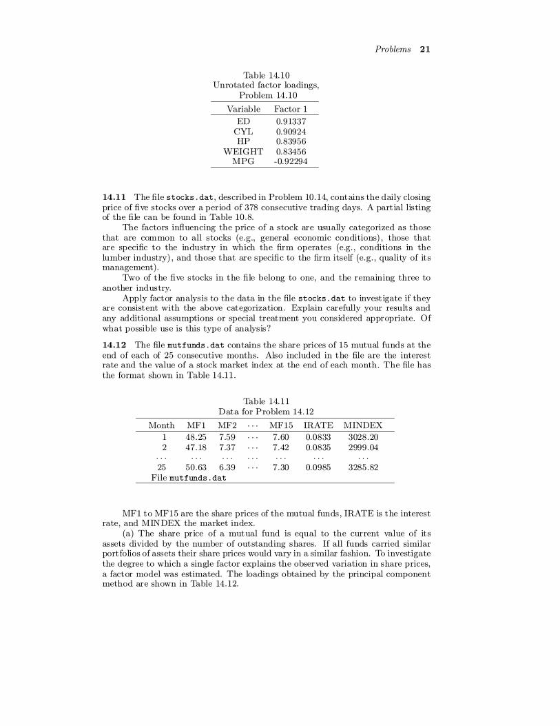
Problems 21
Table 14.10Unrotated factor loadings,
Problem 14.10
Variable Factor 1
ED 0.91337CYL 0.90924HP 0.83956
WEIGHT 0.83456MPG -0.92294
14.11 The ¯le stocks.dat, described in Problem 10.14, contains the daily closingprice of ¯ve stocks over a period of 378 consecutive trading days. A partial listingof the ¯le can be found in Table 10.8.
The factors in°uencing the price of a stock are usually categorized as thosethat are common to all stocks (e.g., general economic conditions), those thatare speci¯c to the industry in which the ¯rm operates (e.g., conditions in thelumber industry), and those that are speci¯c to the ¯rm itself (e.g., quality of itsmanagement).
Two of the ¯ve stocks in the ¯le belong to one, and the remaining three toanother industry.
Apply factor analysis to the data in the ¯le stocks.dat to investigate if theyare consistent with the above categorization. Explain carefully your results andany additional assumptions or special treatment you considered appropriate. Ofwhat possible use is this type of analysis?
14.12 The ¯le mutfunds.dat contains the share prices of 15 mutual funds at theend of each of 25 consecutive months. Also included in the ¯le are the interestrate and the value of a stock market index at the end of each month. The ¯le hasthe format shown in Table 14.11.
Table 14.11Data for Problem 14.12
Month MF1 MF2 ¢ ¢ ¢ MF15 IRATE MINDEX
1 48.25 7.59 ¢ ¢ ¢ 7.60 0.0833 3028.202 47.18 7.37 ¢ ¢ ¢ 7.42 0.0835 2999.04¢ ¢ ¢ ¢ ¢ ¢ ¢ ¢ ¢ ¢ ¢ ¢ ¢ ¢ ¢ ¢ ¢ ¢ ¢ ¢ ¢25 50.63 6.39 ¢ ¢ ¢ 7.30 0.0985 3285.82
File mutfunds.dat
MF1 to MF15 are the share prices of the mutual funds, IRATE is the interestrate, and MINDEX the market index.
(a) The share price of a mutual fund is equal to the current value of itsassets divided by the number of outstanding shares. If all funds carried similarportfolios of assets their share prices would vary in a similar fashion. To investigatethe degree to which a single factor explains the observed variation in share prices,a factor model was estimated. The loadings obtained by the principal componentmethod are shown in Table 14.12.
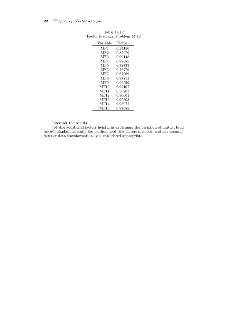
22 Chapter 14: Factor analysis
Table 14.12Factor loadings, Problem 14.12
Variable Factor 1
MF1 0.94156MF2 0.85979MF3 0.99148MF4 0.98685MF5 0.72733MF6 0.76779MF7 0.67069MF8 0.97711MF9 0.92559MF10 0.95107MF11 0.50267MF12 0.90661MF13 0.99303MF14 0.98972MF15 0.97688
Interpret the results.(b) Are additional factors helpful in explaining the variation of mutual fund
prices? Explain carefully the method used, the factors involved, and any assump-tions or data transformations you considered appropriate.