Factor Association using Multiple Correspondence Analysis in Vehicle-pedestrian Crashes 1 2

Subasish Das (Corresponding author) 3

PhD. Student 4

Systems Engineering 5

University of Louisiana 6

Lafayette, LA 70504 7

Email: sxd1684@louisiana.edu 8

Phone: 225-288-9875 9

Fax: 337-739-6688 10

11

12

13

Xiaoduan Sun, Ph.D., and P.E. 14

Professor 15

Civil Engineering Department 16

University of Louisiana 17

Lafayette, LA 70504 18

Email: xsun@louisiana.edu 19

Phone: 337-482-6514 20

Fax: 337-739-6688 21

22

23

24

25

26

27

28

29

30

31

32

33

34

35

36

37

38

39

40

41

42

43

44

45

Word Count: 6,000 including 4 figures and 5 tables 46

47

48

Submitting to the 94th TRB Annual Meetings for Presentation and Publication under 49

Pedestrians Research (ANF10) 50

51

Das, and Sun 2

ABSTRACT 1

2 In the U.S., around 14% of total crash fatalities are pedestrian related. In 2011, 4,432 pedestrians were 3

killed and 69,000 pedestrians were injured in vehicle-pedestrian crashes in the U.S. Vehicle-pedestrian 4

crashes have become a key concern in Louisiana due to the high percentage of fatalities in recent years. In 5

2012, pedestrians accounted for 17% of total crash fatalities in the state. This research uses Multiple 6

Correspondence Analysis (MCA), an exploratory data analysis method used for detecting and 7

representing underlying structures in a categorical data set, to analyze eight years (2004-2011) of vehicle-8

pedestrian crashes in Louisiana. Pedestrian crash data is best represented as transactions of multiple 9

categorical variables, so MCA would be a unique choice to determine the relationship of the variables and 10

their significance. The findings indicated several non-trivial focus groups such as drivers with high 11

occupancy vehicles, female drivers in bad weather conditions, and drivers distracted by mobile phone use. 12

Other key associated factors were hillcrest roadways, dip/hump aligned roadways, roadways with 13

multiple lanes, and roadways with no lighting at night. Male drivers were seen to be more inclined 14

towards severe and moderate injury crashes. Fatal pedestrian crashes were correlated to two-lane 15

roadways with no lighting at night. This method helped to measure significant contributing factors and 16

degrees of association between the factors by analyzing the systematic patterns of variations with 17

categorical datasets of pedestrian crashes. The findings from this study will be helpful for transportation 18

professionals to improve the strategy of counter-measure selection. 19

20

Key words: road safety, single vehicle crashes, fatality, multiple correspondence analysis, cloud of 21

groups, combination. 22

23

24

25

26

27

28

29

30

31

32

33

34

35

36

37

38

39

40

41

42

43

44

45

46

47

48

49

50

51

Das, and Sun 3

INTRODUCTION 1

2 New policies tend to encourage safer and more effective travel for all roadway users in order to make 3

transportation systems more sustainable and efficient. In 2011, 4,432 pedestrians were killed and 69,000 4

pedestrians were injured in vehicle-pedestrian crashes in the United States [1]. Improvement of pedestrian 5

safety is one of the top-most priorities in the American Association of State Highway and Transportation 6

(AASHTO) Strategic Highway Safety Plan (SHSP) [2]. 7

A traffic crash is considered a rare, random, multifactor event always preceded by a state in 8

which one or more roadway users fail to cope with the current environment. Any individual crash is the 9

outcome of a series of events. Although each individual crash is unique in nature, there exists a common 10

occurrence of a few features in several individual crashes [3]. One of the most important tasks in highway 11

safety analysis is the identification of the most significant factors that are related to crashes. Multiple 12

Correspondence Analysis (MCA) is a unique method to present the relative closeness of the categorical 13

variables from any dataset. The traditional hypothesis testing is designed to verify a priori hypotheses 14

regarding relationships between variables, but MCA is used to identify systematic relationships between 15

variables and variable categories with no a priori expectations. The main scope of MCA is that it 16

uniquely simplifies complex data and extracts significant knowledge from the information in the data that 17

assumption-based statistical data analysis fails to collect. Moreover, it has a specific feature similar to 18

multivariate treatment of the data through concurrent considerations of multiple categorical variables that 19

would not be detected in a series of pair-wise comparisons of the variable. As pedestrian crash data can be 20

represented as transactions of multiple categorical variables, MCA would be a good option to determine 21

the relationship of the variables and their significance. 22

The vehicle-pedestrian crash statistics from Louisiana call for instant and advanced solutions to 23

alleviate safety concerns for the pedestrians. The objective of this study was the application of MCA on 24

vehicle-pedestrian crashes to (1) identify the relative closeness of the key association factors, (2) find 25

important nontrivial association between the key factors and (3) provide intuitions to select better 26

countermeasures to improve pedestrian safety. Improving pedestrian safety is crucial to accomplishing the 27

state’s ‘Destination Zero Deaths’ goal and the MCA method used in this paper will help find the relative 28

closeness of the key association factors so that necessary actions can be taken to improve the strategy of 29

pedestrian safety. 30

31

LITERATURE REVIEW 32

33 MCA has been popular in French scientific literature and has obtained a high level of development and 34

use. Although less used in English scientific literature, the method has received increasing attention 35

recently in the field of social science and marketing research. I.P. Benzecri made MCA, a multivariate 36

statistical approach based on the correspondence analysis (CA) method that is popular among scientists. 37

MCA, one of the main standards of geometric data analysis (GDA), is also referred to as the Pattern 38

Recognition Method which treats arbitrary data sets as combination of points in n-dimensional space. 39

However, in the field of multivariate traffic safety data analysis, geometric methods have rarely been 40

used. MCA is hardly utilized in crash analysis. In fact, Roux and Rouanet pointed out that this method, 41

while it is a powerful tool for analyzing a full-scale research database, is still hardly discussed and 42

therefore under-used in many promising fields [4]. 43

Fontaine was the first to use MCA for a typological analysis of pedestrian-related crashes [5]. The 44

classification of pedestrians involved in crashes was divided into four major groups. The typology 45

produced by this analysis revealed correlations between criteria without necessarily indicating a "causal 46

link" with the crashes. The resulting typological breakdown served as a basis for in-depth analysis to 47

improve the understanding of these crashes and propose necessary strategies. Golob and Hensher used 48

MCA to establish causality of nonlinear and non-monotonic relationships between socioeconomic 49

descriptors and measures of travel behavior [6]. Factor et al. conducted a study on the systematical 50

exploration of the homology between drivers’ community characteristics and their involvement in specific 51

Das, and Sun 4

types of vehicle crashes [7]. Das and Sun used the MCA method to analyze eight years (2004-2011) of 1

single-vehicle fatal crashes in Louisiana in order to identify the important contributing factors and their 2

degree of association [8]. 3

Existing literature reveals an extensive variety of contributing factors in vehicle-pedestrian 4

crashes. The key variables associated with vehicle-pedestrian crashes according to the earlier related 5

studies are: higher speed limit (30 mph or over) [9, 10], absence of lighting at night [11], pedestrian 6

visibility [12, 13], and certain age groups [14-15]. 7

After performing a careful investigation on the closely associated research, it is found that a 8

detailed study on the relative closeness of the key association factors of vehicle-pedestrian crashes in the 9

U.S. has not yet been performed. This study attempts to determine the significant combinations of the 10

variables for vehicle-pedestrian crashes by applying MCA which could help state agencies determine 11

effective and efficient crash counter-measures. 12

13

METHODOLOGY 14

15

Theory of MCA 16

The mathematical theory development for MCA is complex in nature. We don’t need to define response 17

and dependable variables. It requires the construction of a matrix based on pairwise cross-tabulation of 18

each variable. For a table with qualitative or categorical variables, MCA can be explained by taking an 19

individual record (in row), i, where three variables (represented by three columns) have three different 20

category indicators (a1, b2, and c3). MCA can generate the spatial distribution of the points by different 21

dimensions based on these three categories. It produces two combinations of points as shown in Figure 1: 22

the combination of individual transactions and the combination of categories [4]. A combination of points 23

can be compared with a geographic map with the same distance scale in all directions. A geometric 24

diagram cannot be strained or contracted along a particular dimension. Thus, the basic property of any 25

combination of points can be known from its dimensionality. Usually the two-dimensional combination is 26

convenient for investigating the points lying on the plane. The complete combinations are generally 27

referred to by their principal dimensions which are ranked in descending order of significance. MCA aims 28

to create a combination of groups put together from a large dataset. The conventional MCA procedure is 29

exhibited in Figure 1. 30

31 Variables from Data 32

33

34

Individual entries (i) 35

Combination of variable categories 36

37

38

39

40

Combination of individual transactions 41

42

FIGURE 1 MCA method. 43

44

First we need to consider P as the number of variables and I as the number of transactions. The 45

matrix will look like “I multiplied by P”, a table for all categorical values. If Tp is the number of 46

a1 b2 c3

..

c3

a1

i

b2

11

Das, and Sun 5

categories for variable p, the total number of categories for all variables is,

P

p pTT1

. We will 1

generate another matrix “I multiplied by T” where each of the variables will have several columns to 2

show all of their possible categorical values. 3

Now we need to consider category k associates with various individual records which can be 4

denoted by nk (nk > 0), where fk = nk/n = relative frequency of individuals associated with k. The values of 5

fk will create a row profile. The distance between two individual records is created by the variables for 6

which both have different categories. For variable p, individual record i contains category k and 7

individual record i contains category k which is different from k. The part of the squared distance 8

between individual records i and i for variable p is 9

)1(11

),(2

kk

pff

iid

10

The overall squared distance between i and i is 11

)2(),(1

),(22

Pp p iidP

iid 12

The set of all distances between individual records determines the combination of individuals 13

consisting of n points in a space. The dimensionality of the space is L, where L ≤ K – P. We assume that 14

n ≥ L. If iM denotes the point representing individual i and G is the mean point of the combination, the 15

squared distance from point iM to point G is defined as 16

)3(11

)( 2

iKkk

i

fPGM 17

where Ki is the response pattern of individual i; that is, the set of the P categories associated with 18

individual record i. 19

The cloud of categories is a weighted combination of K points. Category k is represented by a 20

point denoted by Mk with weight nk. For each variable, the sum of the weights of category points is n, 21

hence for the whole set K the sum is nP. The relative weight wk for point kM is wk = nk/(nP) = fk/P; for 22

each variable, the sum of the relative weights of category points is 1/P, hence for the whole set the sum is 23

1. 24

Kk kKk kkk

k wandp

wwithp

f

np

nw

q

11

25

If kkn denotes the number of individual records which have both of the categories k and k , then 26

the squared distance between kM and

kM is 27

)4(/

2)( 2

nnn

nnnMM

kk

kkkkkk

28

The numerator is the number of individual records associating with either k or k but not both. 29

For two different variables, p and p , the denominator is the familiar "theoretical frequency" for the cell 30

(k, k ) of the pp KK two-way table. 31

The actual computations in MCA are performed on the inner product of this matrix known as the 32

‘Burt Table’. The MCA calculations and two-dimensional plot visualizations in this paper were 33

performed by using open source statistical ‘R Version 3.02’ software [16]. The authors used the 34

‘FactoMineR’ package for its usage convenience to analyze the dataset [17]. The datasets were studied 35

according to the variables and their categories. More emphasis was given to studying the categories, as 36

categories represent both variables and a group of individual records. 37

38

39

Das, and Sun 6

Descriptive Data Analysis 1

To achieve the study objectives, this study used state maintained vehicle-pedestrian crash data compiled 2

from 2004 through 2011 in the state of Louisiana. The primary dataset was prepared by merging three 3

different tables (the crash table, Department of Transportation and Development (DOTD) table and the 4

vehicle table) from the Microsoft Access dataset. The pedestrian dataset was merged again with this 5

merged dataset to get a complete profiling of the pedestrian related crashes. 6

In the crash database, there are numerous variables that are not pertinent to this research, such as: 7

the VIN, driver’s license number, database manager’s name, police report number, etc. In order to focus 8

on the meaningful analysis, a set of key variables were selected, such as: the roadway geometrics 9

(alignment and lighting), collision type, environmental factors (weather), driver-related factors (driver 10

gender, age and condition), number of occupants, and pedestrian-related factors (pedestrian gender, age, 11

condition and severity). The variable section method used the research findings of the previous related 12

research with engineering judgment. 13

An initial analysis indicated that some variables are highly skewed which means that a majority 14

of crashes fall into one of the two or more categorical values. For example, 94% of the crashes involved 15

roadways with straight and level alignment, 76% of the crashes were single-vehicle crashes, and 78% of 16

crashes were single-occupant crashes. From Table 1, it is seen that 61% of pedestrians involved in crashes 17

were male, which was higher than the general trend (around 50 to 55% of traffic crashes involved male 18

drivers in Louisiana). The not-too-skewed variables include collision type, pedestrian injury, and lighting 19

condition. 20

21

Multiple Correspondence Analysis 22

MCA can be explained as a graphical representation by producing a solution in which most associated 23

categories are plotted close together and unassociated ones are plotted far apart. Graphical representations 24

help to perceive and interpret data easily as they effectively summarize large, complex datasets by 25

simplifying the structure of the associations between variables and providing a universal view of the data 26

[4]. Points (categories) that are close to the mean value are plotted near the MCA plot’s origin and those 27

that are more distant are plotted farther away. Categories with a similar distribution are presented near 28

one another by forming combinations, while those with different distributions are plotted some distance 29

apart. Hence, the dimensions are interpreted by the positions of the points on the map, using their loading 30

over the dimensions as crucial indicators. A two-dimensional depiction was sufficient to explain the 31

majority of the variance in Multiple Correspondence Analyses [18]. 32

The eigen values measure indicates how much of the categorical information is accounted for by 33

each dimension. The higher the eigen value, the larger the amount of the total variance among the 34

variables on that dimension. The largest possible eigen value for any dimension is 1. Usually, the first two 35

or three dimensions contain higher eigen values than others. In this analysis, the maximum eigen value in 36

the first dimension (dim 1) was 0.24. The similarly low eigen values in each dimension indicated that the 37

variables in the crash data are heterogeneous and all carry, to some extent, unique information which 38

implies that reducing any of the variables might result in losing important information concerning the 39

crash observations. The heterogeneity of the crash variables reflects the random nature of crash 40

occurrence. 41

In Table 2, eigen values and percentages of variance of the first 10 dimensions are revealed. It 42

can also be seen that there is a steady decrease in eigen values. The first principal axis explained 5.4% of 43

the principal inertia, the second principal axis explained 4.7 % (hence 10.10% in total), and none of the 44

remaining principal axes explained more than 4.7%. As the first plane (with dimensions 1 and 2) 45

represented the largest inertia, only its results were presented and discussed. 46

The coordinates of the first five dimensions for the top ten categories are shown in Table 3. The 47

variables with significance in two dimensions are listed in Table 4. Large coordinate measures indicate 48

that the categories of a variable are better separated along that dimension, while similar coordinate 49

measures for different variables in the same dimensions indicate that these variables are related to each 50

51

Das, and Sun 7

TABLE 1 Distribution of Rainy Weather Crashes by Key Variables 1

Categories Frequency Percentage Categories Frequency Percentage

Alignment (Align.) Pedestrian Injury (Ped. Inj.)

Straight-Level 10750 93.45% Fatal 801 6.96%

Curve-Level 360 3.13% Severe 902 7.84%

On Grade 174 1.51% Moderate 3877 33.70%

Dip, Hump 9 0.08% Complaint 4156 36.13%

Hillcrest 64 0.56% No Injury 1767 15.36%

Unknown (Unk.) 146 1.27% Number of Occupants (Num. Occ.)

Light One 9021 78.42%

Daylight 6272 54.52% Two 1626 14.14%

Dark - No Street Lights 1442 12.54% Three 535 4.65%

Dark - Street Light 3231 28.09% Four 164 1.43%

Dusk, Dawn 358 3.11% Five or more 126 1.10%

Unknown (Unk.) 200 1.74% Unknown (Unk.) 31 0.27%

Collision Number of Lanes (Num. Lanes)

Single Vehicle 4825 41.95% Two 1571 13.66%

Rear End 466 4.05% Four 2102 18.27%

Right Angle 799 6.95% Six 432 3.76%

Right Turn 75 0.65% Eight 16 0.14%

Sideswipe 493 4.29% No Info. 7382 64.17%

Left Turn 209 1.82% Driver Distraction (Dr. Distract)

Head-On 185 1.61% Not Distracted 5888 51.19%

Unknown (Unk.) 4451 38.69% Outside Vehicle 406 3.53%

Weather Cell Phone 83 0.72%

Clear 8770 76.24% Inside Vehi. 158 1.37%

Abnormal 2590 22.52% Electronic Device 10 0.09%

Unknown (Unk.) 143 1.24% Unknown (Unk.) 4958 43.10%

Pedestrian Gender (Ped. Gender)

Female 3738 32.50%

Male 6958 60.49%

Unknown (Unk.) 807 7.02%

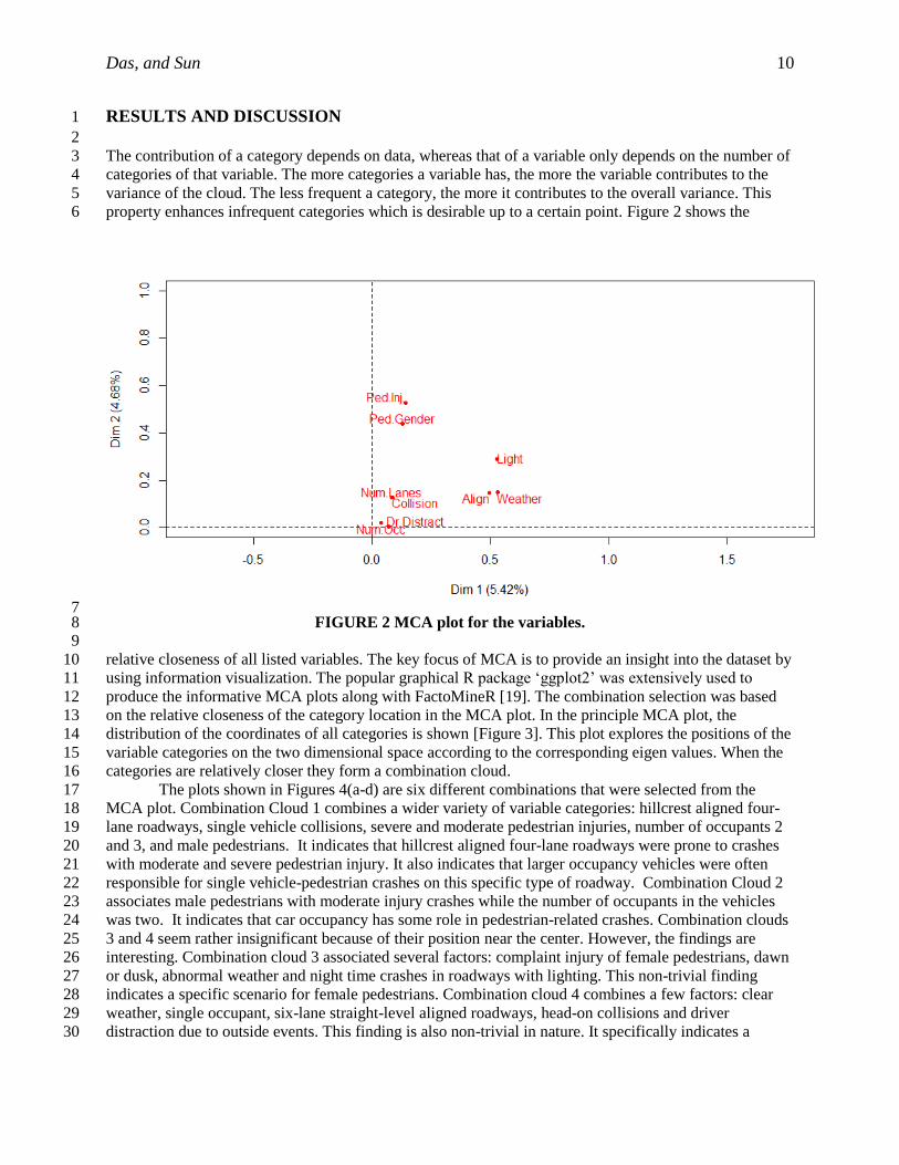
* In the parenthesis, the coded name of the variables is mentioned. 2 3 other. Correlated variables provide redundant information and therefore some of them can be removed. 4

The categories with significance in two dimensions are listed in Table 5. The most discriminant variables 5

for dimension 1 are: weather, alignment, and lighting; regarding dimension 2 the most discriminant 6

variables are: pedestrian injury, pedestrian gender and lighting. By observing the relative closeness of the 7

variables, it is found that the number of lanes, types of collision, driver distraction and number of 8

occupants are closer in the two dimensional space. A more detailed exploration of the variable categories 9

10

11

Das, and Sun 8

TABLE 2 Inertia Values for Top Ten Dimensions 1

Dimensions Eigenvalue Percentage of

Variance

Cumulative Percentage of

Variance

dim 1 0.2349 5.4197 5.4197

dim 2 0.2030 4.6836 10.1032

dim 3 0.1837 4.2394 14.3426

dim 4 0.1346 3.1060 17.4487

dim 5 0.1302 3.0038 20.4525

dim 6 0.1261 2.9091 23.3616

dim 7 0.1223 2.8228 26.1844

dim 8 0.1196 2.7608 28.9452

dim 9 0.1179 2.7210 31.6661

dim 10 0.1172 2.7038 34.3700

TABLE 3 Location of Top Ten Categories in First Five Dimensions 2

Category Dim 1 Dim 2 Dim 3 Dim 4 Dim 5

Align_Curve-Level -0.4630 0.5324 1.1099 -0.7356 0.7293

Align_Dip, Hump 0.2036 -0.5090 -0.5219 0.6853 0.2727

Align_Hillcrest -0.1604 0.4902 1.6002 2.2154 -0.6616

Align_On Grade -0.5258 0.5053 1.3161 0.9319 1.1687

Align_Straight-Level -0.0590 -0.0714 -0.0751 0.0034 -0.0384

Align_Unk 6.1688 3.1579 0.5568 -0.5575 -0.0906

Light_Dark - No Street Lights -0.6664 0.9346 1.2191 -0.4113 0.4166

Light_Dark - Street Light -0.0593 0.0052 0.0581 0.8377 -0.5543

Light_Daylight 0.0262 -0.3069 -0.3174 -0.3048 0.2143

Light_Dusk, Dawn -0.1468 0.0490 -0.1905 -0.1736 -0.2926

TABLE 4 Significance of Key Variables on the First Plane 3

4

MCA Dimension 1 MCA Dimension 1

Variable R2 p.value Variable R2 p.value

Weather 0.5333 0.00E+00 Ped.Inj. 0.5246 0.00E+00

Light 0.5289 0.00E+00 Ped.Gender 0.4393 0.00E+00

Align 0.4973 0.00E+00 Light 0.2891 0.00E+00

Ped.Inj. 0.1415 0.00E+00 Weather 0.1486 0.00E+00

Ped.Gender 0.1298 0.00E+00 Align 0.1456 0.00E+00

Collision 0.0881 8.01E-225 Collision 0.1286 0.00E+00

Num.Lanes 0.0837 3.03E-216 Num.Lanes 0.1260 0.00E+00

Dr.Distract 0.0720 2.39E-183 Num.Occ 0.0216 4.01E-52

Num.Occ 0.0391 6.45E-97 Dr.Distract 0.0033 4.02E-07

5

6

7

Das, and Sun 9

TABLE 5 Significance of Key Categories on the First Plane 1

MCA Dimension 1 MCA Dimension 2

Category Estimate p.value Category Estimate p.value

Weather_Abnormal -1.0697 0.00E+00 Ped.Inj._Unk -1.0316 0.00E+00

Weather_Clear -1.0611 0.00E+00 Ped.Gender_Unk -0.7621 0.00E+00

Light_Dark - No Street Lights -0.7455 0.00E+00 Align_Dip, Hump -0.5375 3.88E-06

Align_On Grade -0.6719 1.33E-106 Weather_Clear -0.5341 0.00E+00

Align_Curve-Level -0.6415 2.63E-129 Weather_Abnormal -0.5018 1.76e-311

Align_Hillcrest -0.4949 4.81E-33 Light_Daylight -0.4443 0.00E+00

Light_Dusk, Dawn -0.4937 6.04E-227 Align_Straight-Level -0.3404 7.96E-38

Light_Dark - Street Light -0.4513 0.00E+00 Collision_Right Turn -0.3071 1.01E-12

Align_Straight-Level -0.4457 1.58E-91 Light_Dark - Street Light -0.3037 3.33E-245

Light_Daylight -0.4099 0.00E+00 Light_Dusk, Dawn -0.2840 5.65E-61

Ped.Inj._Fatal -0.3765 9.13E-154 Num.Lanes_Unk -0.2384 1.05E-14

Num.Occ_Four -0.3579 1.90E-24 Num.Occ_One -0.2114 8.66E-36

Align_Dip, Hump -0.3185 9.12E-04 Dr.Distract_Cell Phone -0.2110 1.13E-05

Num.Occ_Three -0.3141 4.05E-38 Num.Lanes_Six -0.2028 3.67E-14

Num.Occ_Five or more -0.3072 2.43E-15 Collision_Left Turn -0.1798 1.95E-11

Num.Occ_Two -0.2630 2.67E-39 Num.Occ_Five or more -0.1766 1.19E-06

Ped.Gender_Male -0.2398 1.72E-253 Num.Occ_Three -0.1519 2.50E-11

Dr.Distract_Not Distracted -0.2309 5.75E-17 Ped.Inj._No Injury -0.1214 4.16E-44

Ped.Gender_Female -0.2118 2.79E-171 Collision_Rear End -0.1140 2.64E-09

Collision_Single Vehicle -0.1926 1.72E-62 Dr.Distract_Inside Vehi. -0.0975 1.29E-02

Num.Lanes_Two -0.1926 4.76E-14 Num.Occ_Two -0.0817 1.32E-05

Num.Occ_One -0.1732 6.92E-22 Align_On Grade -0.0806 2.82E-02

Dr.Distract_Inside Vehi. -0.1656 4.72E-05 Num.Occ_Four -0.0776 1.81E-02

Dr.Distract_Cell Phone -0.1445 3.76E-03 Align_Curve-Level -0.0684 3.11E-02

Ped.Inj._Severe -0.1097 2.29E-16 Light_Dark - No Street Lights 0.1150 2.04E-27

Dr.Distract_Outside Vehicle -0.0995 2.61E-03 Ped.Inj._Complaint 0.1220 1.10E-109

Ped.Inj._Moderate -0.0897 4.07E-29 Collision_Head-On 0.1234 1.28E-05

Ped.Inj._Complaint -0.0665 2.60E-17 Collision_Unk 0.1271 1.84E-20

Ped.Inj._No Injury 0.0807 1.26E-10 Ped.Inj._Moderate 0.1641 8.76E-187

Num.Lanes_Six 0.1085 2.33E-04 Num.Lanes_Two 0.2096 1.71E-19

Collision_Unk 0.1250 1.16E-16 Ped.Inj._Severe 0.2432 1.84E-148

Num.Lanes_Unk 0.1807 1.01E-07 Num.Lanes_Eight 0.2591 2.15E-03

Ped.Gender_Unk 0.4517 0.00E+00 Dr.Distract_Electronic Device 0.2996 1.19E-02

Ped.Inj._Unk 0.5617 0.00E+00 Ped.Gender_Female 0.3348 0.00E+00

Dr.Distract_Electronic Device 0.6067 9.25E-07 Collision_Single Vehicle 0.3601 1.01E-248

Num.Occ_Unk 1.4155 2.29E-102 Ped.Gender_Male 0.4273 0.00E+00

Light_Unk 2.1003 0.00E+00 Ped.Inj._Fatal 0.6236 0.00E+00

Weather_Unk 2.1307 0.00E+00 Num.Occ_Unk 0.6992 4.46E-30

Align_Unk 2.5724 0.00E+00 Light_Unk 0.9170 0.00E+00

Weather_Unk 1.0358 0.00E+00

Align_Unk 1.1144 8.02E-136

will help more in discovering the underlying structure of the variables. The values from Table 5 indicate 2

that dimension 1 and 2 both were governed by environmental and geometric variable categories. 3

However, the highest estimate for dimension 2 was found for categories of pedestrian injury and gender. 4

5

Das, and Sun 10

RESULTS AND DISCUSSION 1

2

The contribution of a category depends on data, whereas that of a variable only depends on the number of 3

categories of that variable. The more categories a variable has, the more the variable contributes to the 4

variance of the cloud. The less frequent a category, the more it contributes to the overall variance. This 5

property enhances infrequent categories which is desirable up to a certain point. Figure 2 shows the 6

7 FIGURE 2 MCA plot for the variables. 8

9

relative closeness of all listed variables. The key focus of MCA is to provide an insight into the dataset by 10

using information visualization. The popular graphical R package ‘ggplot2’ was extensively used to 11

produce the informative MCA plots along with FactoMineR [19]. The combination selection was based 12

on the relative closeness of the category location in the MCA plot. In the principle MCA plot, the 13

distribution of the coordinates of all categories is shown [Figure 3]. This plot explores the positions of the 14

variable categories on the two dimensional space according to the corresponding eigen values. When the 15

categories are relatively closer they form a combination cloud. 16

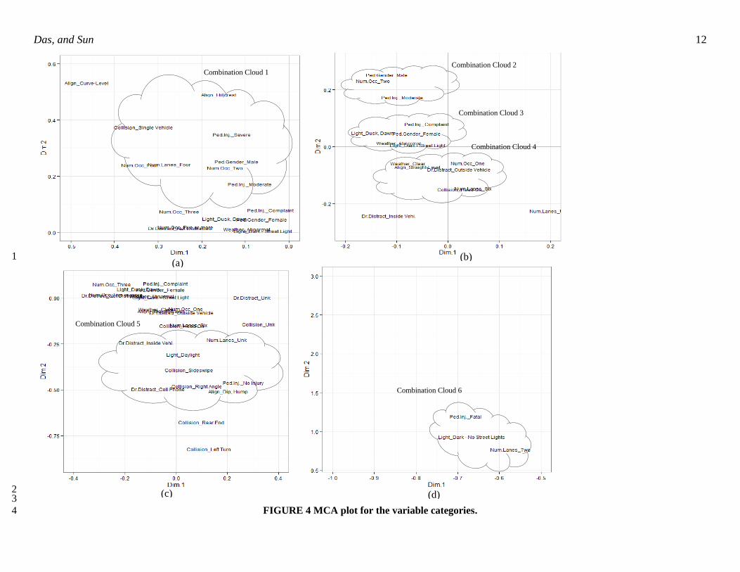
The plots shown in Figures 4(a-d) are six different combinations that were selected from the 17

MCA plot. Combination Cloud 1 combines a wider variety of variable categories: hillcrest aligned four-18

lane roadways, single vehicle collisions, severe and moderate pedestrian injuries, number of occupants 2 19

and 3, and male pedestrians. It indicates that hillcrest aligned four-lane roadways were prone to crashes 20

with moderate and severe pedestrian injury. It also indicates that larger occupancy vehicles were often 21

responsible for single vehicle-pedestrian crashes on this specific type of roadway. Combination Cloud 2 22

associates male pedestrians with moderate injury crashes while the number of occupants in the vehicles 23

was two. It indicates that car occupancy has some role in pedestrian-related crashes. Combination clouds 24

3 and 4 seem rather insignificant because of their position near the center. However, the findings are 25

interesting. Combination cloud 3 associated several factors: complaint injury of female pedestrians, dawn 26

or dusk, abnormal weather and night time crashes in roadways with lighting. This non-trivial finding 27

indicates a specific scenario for female pedestrians. Combination cloud 4 combines a few factors: clear 28

weather, single occupant, six-lane straight-level aligned roadways, head-on collisions and driver 29

distraction due to outside events. This finding is also non-trivial in nature. It specifically indicates a 30

1

2 FIGURE 3 Principle MCA plot for the variable categories. 3

4

5

6

7

8

9

10

11

Das, and Sun 12

1

2 3

FIGURE 4 MCA plot for the variable categories. 4

(a) (b)

Combination Cloud 1

Combination Cloud 5

Combination Cloud 6

Combination Cloud 4

Combination Cloud 3

(d)

Combination Cloud 2

(c)

particular roadway type where distraction happened due to an outside event. Moreover, the crashes 1

involved head-on collisions which also implies involvement with other vehicles. Combination cloud 5 2

also associates different variable categories: driver distraction from mobile or inside equipment, daytime 3

right angle and sideswipe crashes, dip/hump roadways with unknown information on lanes, and PDO 4

pedestrian crashes. This combination indicates cell phone involvement in dip/hump aligned roadways. 5

Combination cloud 6 associates three variable categories: fatal pedestrian crash, nighttime crash, and two-6

lane roadways with no lighting. It indicates that absence of lighting at night is a significant factor for 7

pedestrian traffic severity. This cloud clearly indicates one major focus group on roadway geometrics. 8

The results presented in this paper demonstrate that MCA would be a good option to extract 9

significant knowledge from pedestrian crash data. One of the limitations of the paper is that the findings 10

were based on the two dimensional plane which explained only ten percent of inertia of the data. 11

Explanations on more dimensions would process more knowledge extraction which was not performed in 12

this study. As the initial variable selection was based on the previous research, exploration on other 13

interesting variables was not performed. A more in-depth investigation on the appropriate variables would 14

be a future scope of this research which would help explain a higher percentage of inertia of the data. If 15

the crash database is more complete, MCA will generate more significant combination clouds from the 16

dataset in an unsupervised way. The findings of this research will be helpful to traffic safety professionals 17

in determining the hidden risk association group of variables in fatal single-vehicle crashes. 18

19

CONCLUSION 20

21

Conventional parametric models contain their own model assumptions and pre-defined underlying 22

relationships between dependent and independent variables and assumption violation will lead to the 23

model producing erroneous estimations. The MCA method, a non-parametric method, identifies 24

systematic relationships among variables and variable categories with no a priori assumptions. Moreover, 25

it uniquely simplifies large complex data and represents important knowledge from the dataset. PCA or 26

SOMs are popular tools to describe numerical data; however MCA is a good option for exploratory data 27

analysis for the categorical nature of vehicle-pedestrian crash occurrences. 28

The key focus of this study was to illustrate the applicability of MCA in identifying and 29

representing underlying knowledge in large datasets of vehicle-pedestrian crashes. The findings indicate 30

that MCA helps to cover multiple and diverse variable categories, showing if a relationship exists and 31

how variable categories are related by producing analytical and visual results. Our study identified the 32

groups of drivers and pedestrians as wells as geometric and environmental characteristics that are 33

correlated to vehicle-pedestrian crashes. The findings revealed a few non-trivial risk groups from the 34

analyzed dataset. The key combination groups are- 35

Severe and moderate male pedestrian crashes on hillcrest aligned four-lane roadways associated with 36

single-vehicle collision, and high occupancy vehicles (occupancy= 2 and 3). 37

Moderate male pedestrian crashes when the occupancy of the vehicle is two. 38

Complaint female pedestrian crashes associated with dawn or dusk, abnormal weather and night-time 39

crashes in roadways with lighting. 40

Head-on collisions on six-lane straight-level aligned roadways associated with single occupant, clear 41

weather, single occupancy, and driver distraction happened due to outside events. 42

PDO pedestrian crashes on dip/hump roadways due to drivers’ distraction from mobile phones 43

accompanying with daytime right angle and sideswipe crashes, and unknown information on lanes. 44

Fatal pedestrian crashes on two-lane roadways with no lighting at night. It implies that pedestrian 45

behavior in darkness is a continuing traffic safety issue. 46

In particular the ability of MCA to deal with multidimensional data makes it particularly useful for 47

exploring the factors influencing crash occurrences. The findings from this research shed light on the 48

pattern recognition of vehicle-pedestrian crashes and expose new aspects in pedestrian safety and also 49

point to potential future research considering more variables and large datasets from multiple states. The 50

Das, and Sun 14

findings may seem trivial in places, but the findings are based on extensive data exploration method to 1

execute statistically significant valid combination groups. So, the jurisdictions can take appropriate 2

actions on the strategies for the combination groups. Crashes dominated by human factors can be 3

scrutinized by exploring the current law and safety education system. Modifications in laws can be made 4

to make the drivers and pedestrian less vulnerable to crashes. Associated geometric features can be 5

examined for the safety performance and improvement can be done accordingly. 6

7

8

REFERENCES 9

10

[1] Schneider, H. Louisiana Traffic Records Data Report 2013. Louisiana State University, Baton 11

Rouge, Louisiana, 2014. 12

[2] Strategic Highway Safety Plan. A Comprehensive Plan to Substantially Reduce Vehicle- 13

Related Fatalities and Injuries on the Nation’s Highways. AASHTO, Washington, D.C., 14

2005. 15

[3] Montella, A. Identifying Crash Contributory Factors at Urban Roundabouts and Using 16

Association Rules to Explore Their Relationships to Different Crash Types. Accident 17

Analysis and Prevention, 43(4), pp. 1451–1463, 2011. 18

[4] Roux B., and Rouanet H. Multiple Correspondence Analysis. Sage Publications, 19

Washington D.C. 2010. 20

[5] Fontaine H. A Typological Analysis of Pedestrian Accidents. Presented at the 7th 21

workshop of ICTCT, Paris, 26-27 October, 1995. 22

[6] Golob TF, Hensher DA. The trip chaining activity of Sydney residents: A cross-section assessment 23

by age group with a focus on seniors. Journal of Transport Geography. 2007; 15(4). 24

[7] Factor R, Yair G, and Mahalel, D. Who by Accident? The Social Morphology of Car 25

Accidents. Risk Analysis. 2010; 30(9). 26

[8] Das S, and Sun X.Yair G, Mahalel, D. Exploring Clusters of Contributing Factors for Single-Vehicle 27

Fatal Crashes Through Multiple Correspondence Analysis. TRB 93rd Annual Meeting Compendium 28

of Papers, Washington DC, 2014. 29

[9] Davis, G. Relating severity of pedestrian injury to impact speed in vehicle–pedestrian 30

crashes: simple threshold model. Transportation Research Record: Journal of the 31

Transportation Research Board, 1773 (1), pp. 108–113, 2001. 32

[10] Sze, N., and Wong, S. 2007. Diagnostic analysis of the logistic model for pedestrian 33

Injury severity in traffic crashes. Accident Analysis and Prevention, 39 (6), pp. 1267– 34

1278, 2007. 35

[11] Moudon, A., Lin, L., Jiao, J., Hurvitz, P., and Reeves, P. The risk of pedestrian injury and 36

fatality in collisions with motor vehicles, a social ecological study of state routes and 37

city streets in King County, Washington. Accident Analysis and Prevention 43 (1), pp. 38

11–24, 2011. 39

[12] Ulfarsson, G., Kim, S., and Booth, K. Analyzing fault in pedestrian–motor vehicle 40

crashes in North Carolina. Accident Analysis and Prevention 42 (6), pp. 1805–1813, 41

2010. 42

[13] Sullivan, J., and Flannagan, M. Differences in geometry of pedestrian crashes in 43

daylight and darkness. Journal of Safety Research 42 (1), pp. 33–37, 2011. 44

[14] Roudsari, B., Mock, C., Kaufman, R., Grossman, D., Henary, B., and Crandall, J. 45

Pedestrian crashes: higher injury severity and mortality rate for light truck vehicles 46

compared with passenger vehicles. Injury Prevention 10 (3), pp. 154–158, 2004. 47

[15] Eluru, N., Bhat, C., and Hensher, D. A mixed generalized ordered response model 48

for examining pedestrian and bicyclist injury severity level in traffic crashes. Accident 49

Analysis and Prevention 40 (3), pp. 1033–1054, 2008. 50

[16] R Core Team. R: A language and environment for statistical computing. R Foundation 51

Das, and Sun 15

for Statistical Computing, Vienna, Austria. http://www.R-project.org. Accessed July 1

20, 2013. 2

[17] Husson F, Josse J, Le, S., and Mazet J. FactoMineR: Multivariate Exploratory Data 3

Analysis and Data Mining with R. R package version 1.25. http://CRAN.R- 4

project.org/package=FactoMineR. Accessed July 21, 2014. 5

[18] Greenacre, M., and Blasius J. Multiple Correspondence Analysis and Related Methods. 6

Chapman & Hall/CRC, FL, 2006. 7

[19] Wickham H. ggplot2: elegant graphics for data analysis. Springer New York, 2009. 8