Computational Water, Energy, and Environmental Engineering, 2016, 5, 10-26 Published Online January 2016 in SciRes. http://www.scirp.org/journal/cweee http://dx.doi.org/10.4236/cweee.2016.51002

How to cite this paper: Okweye, P.S., Garner, K.G., Overton, A.S. and Moss, E.M. (2016) Factor-Cluster Analysis and Effect of Particle Size on Total Recoverable Metal Concentration in Sediments of the Lower Tennessee River Basin. Computational Water, Energy, and Environmental Engineering, 5, 10-26. http://dx.doi.org/10.4236/cweee.2016.51002

Factor-Cluster Analysis and Effect of Particle Size on Total Recoverable Metal Concentration in Sediments of the Lower Tennessee River Basin Paul S. Okweye1*, Karnita G. Garner2, Anthony S. Overton2, Elica M. Moss2 1College of Engineering, Technology & Physical Sciences, Department of Physics, Chemistry and Mathematics, Alabama A&M University, Normal, AL, USA 2College of Agricultural, Life and Natural Sciences, Department of Biology and Environmental Sciences, Alabama A&M University, Normal, AL, USA

Received 6 June 2015; accepted 25 January 2016; published 29 January 2016

Copyright © 2016 by authors and Scientific Research Publishing Inc. This work is licensed under the Creative Commons Attribution International License (CC BY). http://creativecommons.org/licenses/by/4.0/

Abstract Total recoverable concentration of five elements of concern: Aluminum, Iron, Manganese, Arsenic and Lead (Al, Fe, Mn, As, Pb) were measured by inductively coupled plasma atomic emission spec-trometry, and mass spectrometry. The results show that sediment texture plays a controlling role in the concentrations and their spatial distribution. Principal Component Analysis and Cluster Analysis were used to analyze the grain sizes of the sediments. Result of texture analysis classified the samples into three main components in percentages: sand, silt, and clay. Significant differenc-es among the element concentrations in the three groups were observed, and the concentrations of the elements in each group are reported in this study. Most of the elements have their highest concentrations in the fine-grained samples with clay playing an important role, in comparison with the sand component of the soil/sediment samples. There appears to be a strong correlation between samples with high silt, and clay content with the areas of elevated concentrations for Al, Fe, and Mn. There was a strong correlation between aluminum and lead with clay; lead with silt; and sand with manganese, aluminum, and lead. However, there was no strong relationship be-tween the soil textures and iron or arsenic. All elements measured were statistically significant (at P ≤ 0.05) by watershed. The upland areas, and depositional areas’ spatial variation of element concentrations in the sediments were also observed, which was in line with the spatial distribu-

*Corresponding author.

P. S. Okweye et al.

11

tion of the grain size and was thought to be related to the watersheds hydrological dynamics.

Keywords Total Recoverable Metals, Principal Component Analysis, Cluster Analysis, Correlation, Hydrological Dynamics

1. Introduction Lower Tennessee River basin in Alabama includes the Flint Creek (FC) and Flint River (FR) watersheds, and the spatial distribution of the grain size of sediments at these watersheds is largely fine grained in the upper, middle to lower reaches of the rivers. To study the grain size effect on the total recoverable metal concentrations in sediments, samples within, and along the river, sites were collected in winter/spring of 2014. Sediments in ri-verbeds serve as depositories for most aquatic pollutants, including heavy metals. Hence sediments are consi-dered to be an important indicator for environmental pollution [1]. Sediments act as sinks and sources of conta-minants in aquatic systems because of their variable physical and chemical properties [2]. Heavy metals in se-diments in the Flint Creek (FC) and the Flint River (FR) watersheds in the Tennessee River (TR) basin have re-ceived very little scientific attention. Okweye et al. [3] concluded that the surface water from the FC and the FR watersheds in the TR basin had been polluted with heavy metals from anthropogenic sources surrounding the watersheds. Furthermore, the concentrations of heavy metals in the soil/sediment of these watersheds exceeded the maximum contaminant level (MCL) allowed by USEPA in drinking water. This paper examines the concen-trations of heavy metals (Al, Fe, Mn, As, and Pb) in relation to sediment grain size distribution on the water-sheds. Particle size is important because the grain size of soil particles and their aggregate structures affect the ability of soil to transport and retain water and nutrients.

The purpose of this study was: 1) to determine the distribution of the particle size of the soil/sediment and heavy metals (Al, Fe, Mn, As, and Pb) at depositional and upland areas of each site; and 2) to identify the con-trolling factors by using Principal Component Analysis (PCA) and Cluster Analysis (CA) because multivariate analyses are useful for interpreting elements in spatial patterns, which might be related to similar input sources or transport pathways [4].

The study tested the null hypothesis that soil/sediment particle size distribution and sampling location influenced the level of heavy metal concentration within the watersheds. The results from this study are expected to provide a framework for interpreting sediment toxicity and group elements with similar properties at these watersheds.

2. Materials and Method 2.1. Study Area and Location of Sampling Sites Table 1. Showing the Flint Creek (FC) and Flint River (FR) Geographic Point Coordinates (GIS).

FR Latitude Longitude

WR-FR N34˚49'25.932'' W086˚28'59.081''

BF-FR N34˚49'25.915'' W086˚29'6.778''

HR-FR N34˚32'3.822'' W086˚29'59.782''

FC Latitude Longitude

RB-FC N34˚30'30.264'' W086˚57'30.264''

MB-FC N34˚27'49.038'' W086˚58'41.844''

VB-FC N34˚29'50.894'' W087˚01'3.679''

FR (codes: WR-FR = Winchester Road, BF-FR = Briar Fork, HR-FR = Hobbs Road); FC (Codes: RB-FC = Red Bank, MB-FC = Means Bridge, VB-FC = Vaughn Bridge).

P. S. Okweye et al.

12

(a)

(b)

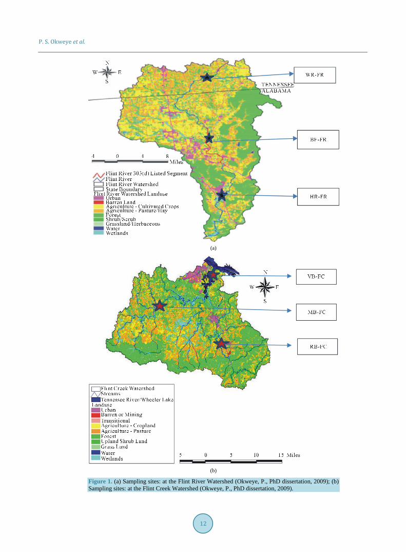
Figure 1. (a) Sampling sites: at the Flint River Watershed (Okweye, P., PhD dissertation, 2009); (b) Sampling sites: at the Flint Creek Watershed (Okweye, P., PhD dissertation, 2009).

P. S. Okweye et al.

13

Table 2. Soil Types for the FC and FR Watersheds (Courtesy: Joe Gardinski, NRCS).

FR Code Soil Types

WR-FR Ennis silt loam

BF-FR Bodine cherty silt loam

HR-FR Melvin silty clay loam

FC Code Soil Types

RB-FC Bruno loamy fine sand

MB-FC Lindside silty clay loam

VB-FC Muskingum stony fine sandy loam

2.2. Sample Collection Soil/sediment samples were collected in winter/spring 2014 from six sites (WR-FR, BF-FR, HR-FR, RB-FC, MB-FC, and VB-FC) as shown in Figure 1(a); Figure 1(b) and Table 1. Samples were transferred into sam-pling bags and placed in a cooler at 4˚C, and then transported to Alabama A&M University laboratories for sto-rage. About 1 kg of sample was obtained from each site and air dried before analysis. All the sampling locations were recorded with a GPS. Most of the samples were fine-grained clay and silt, and passed through a 1 mm metal sieve.

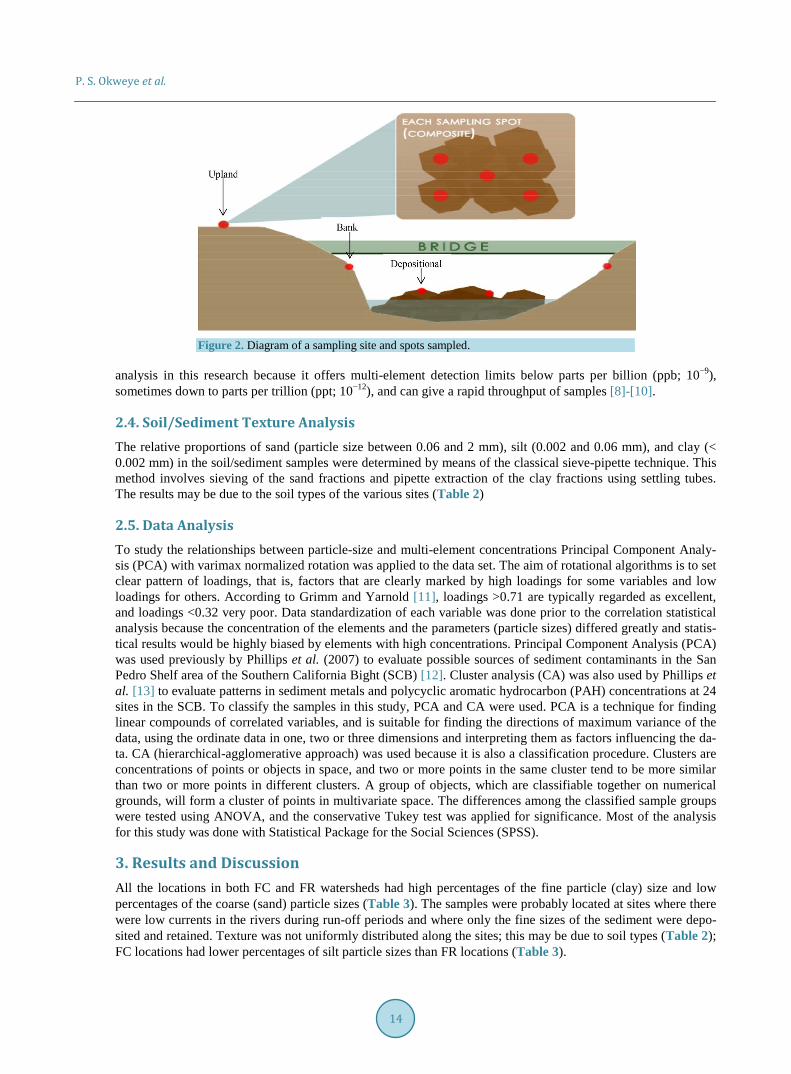
The soil/sediment sampling locations for each site included: 1) an in-stream/Depositional area, 2) a Bank-side, and 3) an Upland in riparian zone. At each location, five samples were collected, composited, and well-mixed to obtain a representative sample (Figure 2). A stainless steel soil probe was used to collect soils from the banks and upland areas, and a 250-cm pole sediment sampler—Pakar [5] was used for collecting sediments from in- stream/depositional areas across the upper, middle, and lower sections of the streams, covering a distance of ~110 km. The sediment sampling was carried out in low flow conditions because trace metal concentrations tend to be highest during this period as metals accumulate in the sediments from water. Under high water discharge, erosion of riverbeds takes place. According to the UNEP/WHO [6], following peak discharge, the concentra-tions of metals in bed sediments increase as the water flow again decreases. A total of seventy-two (72) soil/ se-diment samples were collected from the watersheds. In the laboratory, samples were stored in the freezer until they were processed and analyzed. In-situ measurements for physical and chemical characteristics of water and soil properties were conducted at the sites with a 6600 Extended Deployment System (EDS).

2.3. Analytical Methods USEPA Method 3050B [7] was used for the digestion of heavy metals in soil/sediment samples at the Environ-mental Testing and Consulting (ETC) laboratories in Memphis, Tennessee. This method is suitable for hot block digestion of soil, sediment, and waste samples and for analysis by inductively coupled plasma optical emis-sion/atomic emission spectrometry (ICP-OES/AES). A 1.0 g subsample of each sample was digested in nitric acid and hydrogen peroxide. The digestate was then further refluxed with hydrochloric acid. High-tech instru-ment ICP-AES, with SW-846 USEPA method 6010B, was used for the elemental determination. The USEPA standard sediment samples were used to monitor the analyses. Al, Fe, Mn, and Pb was measured by inductively coupled plasma optical emission spectrometry (ICP-OES, Optima 2000DV; Perkin Elmer, Waltham, MA, USA; detection limit 0.001 - 0.030 mg/L) and inductively coupled plasma-mass spectrometry (ICP-MS, 7500a; Agi-lent Technologies, Santa Clara, CA, USA; detection limit 0.015 - 0.120 mg/L) was used for the analysis for Ar-senic (As). Laboratory quality control consisted of analysis of sediment reference material (GBW 07302- 07312a; National Institute of Standard and Technology, MD, USA) and triplicate samples were used. The results were consistent with the reference values, and the differences were generally within 10% (most were within 5%).

The recoveries all fell within the range of 90% - 110%, and the relative standard deviation was less than 5%. All The reagents used for the analysis were AR grade and double distilled water was used for preparation of so-lutions. The analyzing laboratory - ETC asserted that the results from the average values of the concentrations of the elements detected by both ICP-OES/AES (Al, Fe, Mn, and Pb) and ICP-MS (As) were consistent. The qual-ity control in this study was similar to that used in a previous study in the area [3]. ICP-MS was used for arsenic

P. S. Okweye et al.

14

Figure 2. Diagram of a sampling site and spots sampled.

analysis in this research because it offers multi-element detection limits below parts per billion (ppb; 10−9), sometimes down to parts per trillion (ppt; 10−12), and can give a rapid throughput of samples [8]-[10].

2.4. Soil/Sediment Texture Analysis The relative proportions of sand (particle size between 0.06 and 2 mm), silt (0.002 and 0.06 mm), and clay (< 0.002 mm) in the soil/sediment samples were determined by means of the classical sieve-pipette technique. This method involves sieving of the sand fractions and pipette extraction of the clay fractions using settling tubes. The results may be due to the soil types of the various sites (Table 2)

2.5. Data Analysis To study the relationships between particle-size and multi-element concentrations Principal Component Analy-sis (PCA) with varimax normalized rotation was applied to the data set. The aim of rotational algorithms is to set clear pattern of loadings, that is, factors that are clearly marked by high loadings for some variables and low loadings for others. According to Grimm and Yarnold [11], loadings >0.71 are typically regarded as excellent, and loadings <0.32 very poor. Data standardization of each variable was done prior to the correlation statistical analysis because the concentration of the elements and the parameters (particle sizes) differed greatly and statis-tical results would be highly biased by elements with high concentrations. Principal Component Analysis (PCA) was used previously by Phillips et al. (2007) to evaluate possible sources of sediment contaminants in the San Pedro Shelf area of the Southern California Bight (SCB) [12]. Cluster analysis (CA) was also used by Phillips et al. [13] to evaluate patterns in sediment metals and polycyclic aromatic hydrocarbon (PAH) concentrations at 24 sites in the SCB. To classify the samples in this study, PCA and CA were used. PCA is a technique for finding linear compounds of correlated variables, and is suitable for finding the directions of maximum variance of the data, using the ordinate data in one, two or three dimensions and interpreting them as factors influencing the da-ta. CA (hierarchical-agglomerative approach) was used because it is also a classification procedure. Clusters are concentrations of points or objects in space, and two or more points in the same cluster tend to be more similar than two or more points in different clusters. A group of objects, which are classifiable together on numerical grounds, will form a cluster of points in multivariate space. The differences among the classified sample groups were tested using ANOVA, and the conservative Tukey test was applied for significance. Most of the analysis for this study was done with Statistical Package for the Social Sciences (SPSS).

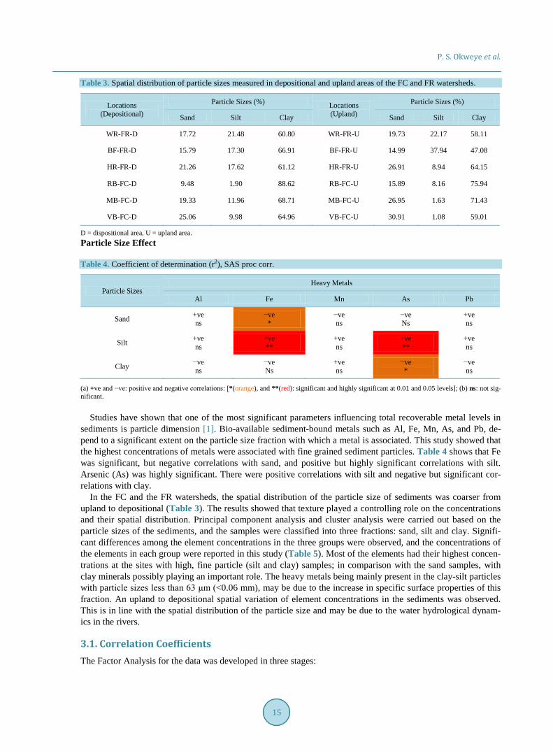
3. Results and Discussion All the locations in both FC and FR watersheds had high percentages of the fine particle (clay) size and low percentages of the coarse (sand) particle sizes (Table 3). The samples were probably located at sites where there were low currents in the rivers during run-off periods and where only the fine sizes of the sediment were depo-sited and retained. Texture was not uniformly distributed along the sites; this may be due to soil types (Table 2); FC locations had lower percentages of silt particle sizes than FR locations (Table 3).

P. S. Okweye et al.

15

Table 3. Spatial distribution of particle sizes measured in depositional and upland areas of the FC and FR watersheds.

Locations (Depositional)

Particle Sizes (%) Locations (Upland)

Particle Sizes (%)

Sand Silt Clay Sand Silt Clay

WR-FR-D 17.72 21.48 60.80 WR-FR-U 19.73 22.17 58.11

BF-FR-D 15.79 17.30 66.91 BF-FR-U 14.99 37.94 47.08

HR-FR-D 21.26 17.62 61.12 HR-FR-U 26.91 8.94 64.15

RB-FC-D 9.48 1.90 88.62 RB-FC-U 15.89 8.16 75.94

MB-FC-D 19.33 11.96 68.71 MB-FC-U 26.95 1.63 71.43

VB-FC-D 25.06 9.98 64.96 VB-FC-U 30.91 1.08 59.01

D = dispositional area, U = upland area. Particle Size Effect Table 4. Coefficient of determination (r2), SAS proc corr.

Particle Sizes Heavy Metals

Al Fe Mn As Pb

Sand +ve ns

−ve *

−ve ns

−ve Ns

+ve ns

Silt +ve ns

+ve **

+ve ns

+ve **

+ve ns

Clay −ve ns

−ve Ns

+ve ns

−ve *

−ve ns

(a) +ve and −ve: positive and negative correlations: [*(orange), and **(red): significant and highly significant at 0.01 and 0.05 levels]; (b) ns: not sig-nificant.

Studies have shown that one of the most significant parameters influencing total recoverable metal levels in sediments is particle dimension [1]. Bio-available sediment-bound metals such as Al, Fe, Mn, As, and Pb, de-pend to a significant extent on the particle size fraction with which a metal is associated. This study showed that the highest concentrations of metals were associated with fine grained sediment particles. Table 4 shows that Fe was significant, but negative correlations with sand, and positive but highly significant correlations with silt. Arsenic (As) was highly significant. There were positive correlations with silt and negative but significant cor-relations with clay.

In the FC and the FR watersheds, the spatial distribution of the particle size of sediments was coarser from upland to depositional (Table 3). The results showed that texture played a controlling role on the concentrations and their spatial distribution. Principal component analysis and cluster analysis were carried out based on the particle sizes of the sediments, and the samples were classified into three fractions: sand, silt and clay. Signifi-cant differences among the element concentrations in the three groups were observed, and the concentrations of the elements in each group were reported in this study (Table 5). Most of the elements had their highest concen-trations at the sites with high, fine particle (silt and clay) samples; in comparison with the sand samples, with clay minerals possibly playing an important role. The heavy metals being mainly present in the clay-silt particles with particle sizes less than 63 μm (<0.06 mm), may be due to the increase in specific surface properties of this fraction. An upland to depositional spatial variation of element concentrations in the sediments was observed. This is in line with the spatial distribution of the particle size and may be due to the water hydrological dynam-ics in the rivers.

3.1. Correlation Coefficients The Factor Analysis for the data was developed in three stages:

P. S. Okweye et al.

16

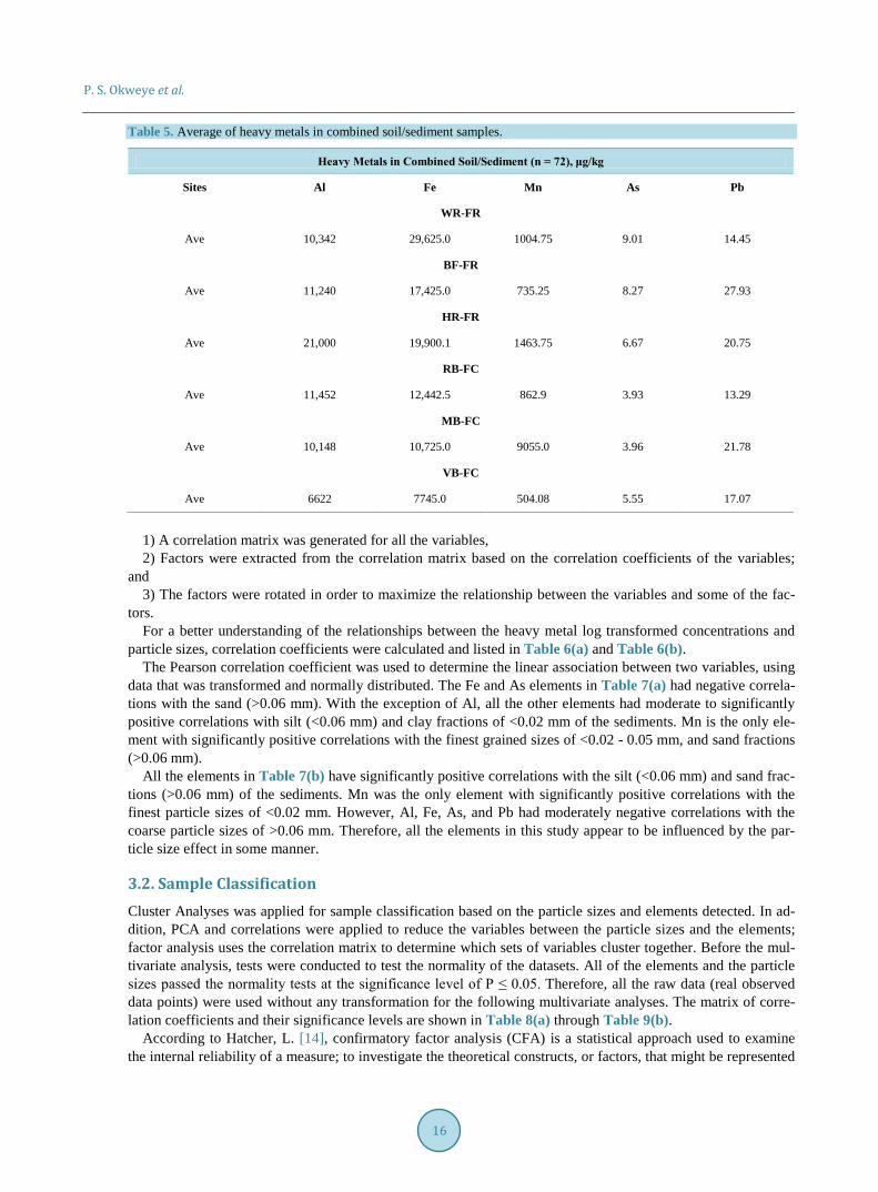
Table 5. Average of heavy metals in combined soil/sediment samples.

Heavy Metals in Combined Soil/Sediment (n = 72), μg/kg

Sites Al Fe Mn As Pb

WR-FR

Ave 10,342 29,625.0 1004.75 9.01 14.45

BF-FR

Ave 11,240 17,425.0 735.25 8.27 27.93

HR-FR

Ave 21,000 19,900.1 1463.75 6.67 20.75

RB-FC

Ave 11,452 12,442.5 862.9 3.93 13.29

MB-FC

Ave 10,148 10,725.0 9055.0 3.96 21.78

VB-FC

Ave 6622 7745.0 504.08 5.55 17.07

1) A correlation matrix was generated for all the variables, 2) Factors were extracted from the correlation matrix based on the correlation coefficients of the variables;

and 3) The factors were rotated in order to maximize the relationship between the variables and some of the fac-

tors. For a better understanding of the relationships between the heavy metal log transformed concentrations and

particle sizes, correlation coefficients were calculated and listed in Table 6(a) and Table 6(b). The Pearson correlation coefficient was used to determine the linear association between two variables, using

data that was transformed and normally distributed. The Fe and As elements in Table 7(a) had negative correla-tions with the sand (>0.06 mm). With the exception of Al, all the other elements had moderate to significantly positive correlations with silt (<0.06 mm) and clay fractions of <0.02 mm of the sediments. Mn is the only ele-ment with significantly positive correlations with the finest grained sizes of <0.02 - 0.05 mm, and sand fractions (>0.06 mm).

All the elements in Table 7(b) have significantly positive correlations with the silt (<0.06 mm) and sand frac-tions (>0.06 mm) of the sediments. Mn was the only element with significantly positive correlations with the finest particle sizes of <0.02 mm. However, Al, Fe, As, and Pb had moderately negative correlations with the coarse particle sizes of >0.06 mm. Therefore, all the elements in this study appear to be influenced by the par-ticle size effect in some manner.

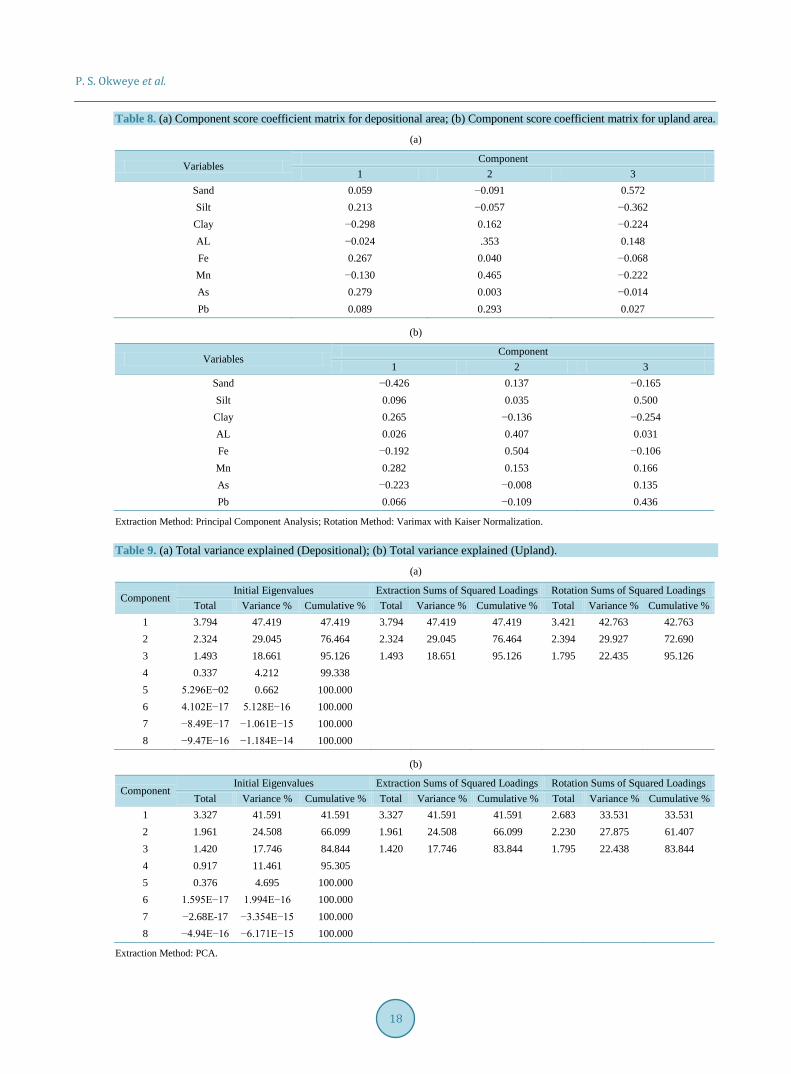
3.2. Sample Classification Cluster Analyses was applied for sample classification based on the particle sizes and elements detected. In ad-dition, PCA and correlations were applied to reduce the variables between the particle sizes and the elements; factor analysis uses the correlation matrix to determine which sets of variables cluster together. Before the mul-tivariate analysis, tests were conducted to test the normality of the datasets. All of the elements and the particle sizes passed the normality tests at the significance level of P ≤ 0.05. Therefore, all the raw data (real observed data points) were used without any transformation for the following multivariate analyses. The matrix of corre-lation coefficients and their significance levels are shown in Table 8(a) through Table 9(b).

According to Hatcher, L. [14], confirmatory factor analysis (CFA) is a statistical approach used to examine the internal reliability of a measure; to investigate the theoretical constructs, or factors, that might be represented

P. S. Okweye et al.

17

Table 6. (a) Pearson correlation coefficients for depositional areas; (b) Pearson correlation coefficients (upland–reference area).

(a)

Log-Sand Log-Silt Log-Clay Log-AL Log-Fe Log-Mn Log-As Log-Pb

Log-Sand 1.000

Log-Silt −0.575** 1.000

Log-Clay 0.517 −0.562** 1.000

Log-Al 0.398 −0.452* 0.417 1.000

Log-Fe −0.462* 0.326 0.655 0.748 1.000

Log-Mn 0.869 0.613 0.359 0.338 0.554 1.000

Log-As −0.417* 0.277 0.595 0.738 0.969** 0.510 1.000

Log-Pb 0.707 0.517 0.528 0.748** 0.390 0.647** 0.397 1.000

(b)

Log-Sand Log-Silt Log-Clay Log-AL Log-Fe Log-Mn Log-As Log-Pb

Log-Sand 1.000

Log-Silt 0.302 1.000

Log-Clay −0.615** −0.764** 1.000

Log-Al 0.560 0.660 −0.290 1.000

Log-Fe 0.246 0.272 −0.452* 0.882** 1.000

Log-Mn 0.251 0.893 0.828 0.851** 0.618** 1.000

Log-As 0.357 0.354 −0.450* 0.259 0.554** 0.666 1.000

Log-Pb 0.481 0.361 −0.256 0.537 0.355 0.966 0.651 1.000 *= Correlation is significant at the 0.05 level (2-tailed); **= Correlation is significant at the 0.01 level (2-tailed). Table 7. (a) Correlation matrix for depositional areas; (b) Correlation matrix for upland areas.

(a)

Sand Silt Clay AL Fe Mn As Pb

Sand 1.000

Silt −0.583 1.000

Clay −0.447 −0.466 1.000

AL 0.496 −0.295 −0.216 1.000

Fe 0.016 0.695 −0.782 0.340 1.000

Mn −0.110 −0.030 0.152 0.740 0.155 1.000

As 0.074 0.638 −0.783 0.306 0.949 0.026 1.000

Pb 0.251 0.091 −0.373 0.828 0.640 0.541 0.704 1.000

(b)

Sand Silt Clay AL Fe Mn As Pb

Sand 1.000

Silt −0.186 1.000

Clay −0.653 −0.623 1.000

AL −0.315 0.105 0.170 1.000

Fe 0.087 0.039 −0.099 0.877 1.000

Mn −0.743 0.110 0.507 0.815 0.451 1.000

As 0.549 0.088 −0.505 −0.357 −0.103 −0.461 1.000

Pb 0.168 0.301 −0.366 −0.144 −0.267 0.059 0.487 1.000

P. S. Okweye et al.

18

Table 8. (a) Component score coefficient matrix for depositional area; (b) Component score coefficient matrix for upland area.

(a)

Variables Component

1 2 3 Sand 0.059 −0.091 0.572 Silt 0.213 −0.057 −0.362 Clay −0.298 0.162 −0.224 AL −0.024 .353 0.148 Fe 0.267 0.040 −0.068 Mn −0.130 0.465 −0.222 As 0.279 0.003 −0.014 Pb 0.089 0.293 0.027

(b)

Variables Component

1 2 3 Sand −0.426 0.137 −0.165 Silt 0.096 0.035 0.500 Clay 0.265 −0.136 −0.254 AL 0.026 0.407 0.031 Fe −0.192 0.504 −0.106 Mn 0.282 0.153 0.166 As −0.223 −0.008 0.135 Pb 0.066 −0.109 0.436

Extraction Method: Principal Component Analysis; Rotation Method: Varimax with Kaiser Normalization. Table 9. (a) Total variance explained (Depositional); (b) Total variance explained (Upland).

(a)

Component Initial Eigenvalues Extraction Sums of Squared Loadings Rotation Sums of Squared Loadings

Total Variance % Cumulative % Total Variance % Cumulative % Total Variance % Cumulative % 1 3.794 47.419 47.419 3.794 47.419 47.419 3.421 42.763 42.763 2 2.324 29.045 76.464 2.324 29.045 76.464 2.394 29.927 72.690 3 1.493 18.661 95.126 1.493 18.651 95.126 1.795 22.435 95.126 4 0.337 4.212 99.338 5 5.296E−02 0.662 100.000 6 4.102E−17 5.128E−16 100.000 7 −8.49E−17 −1.061E−15 100.000 8 −9.47E−16 −1.184E−14 100.000

(b)

Component Initial Eigenvalues Extraction Sums of Squared Loadings Rotation Sums of Squared Loadings

Total Variance % Cumulative % Total Variance % Cumulative % Total Variance % Cumulative % 1 3.327 41.591 41.591 3.327 41.591 41.591 2.683 33.531 33.531 2 1.961 24.508 66.099 1.961 24.508 66.099 2.230 27.875 61.407 3 1.420 17.746 84.844 1.420 17.746 83.844 1.795 22.438 83.844 4 0.917 11.461 95.305 5 0.376 4.695 100.000 6 1.595E−17 1.994E−16 100.000 7 −2.68E-17 −3.354E−15 100.000 8 −4.94E−16 −6.171E−15 100.000

Extraction Method: PCA.

P. S. Okweye et al.

19

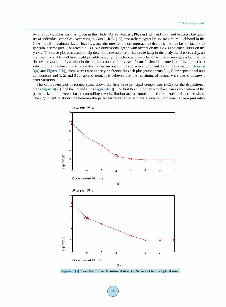
by a set of variables, such as, given in this study (Al, Fe, Mn, As, Pb, sand, silt, and clay) and to assess the qual-ity of individual variables. According to Cattell, R.B. [15], researchers typically use maximum likelihood in the CFA model to estimate factor loadings, and the most common approach to deciding the number of factors to generate a scree plot. The scree plot is a two dimensional graph with factors on the x-axis and eigenvalues on the y-axis. The scree plot was used to help determine the number of factors to keep in the analysis. Theoretically, an eight-item variable will have eight possible underlying factors, and each factor will have an eigenvalue that in-dicates the amount of variation in the items accounted for by each factor. It should be noted that this approach to selecting the number of factors involved a certain amount of subjective judgment. From the scree plot (Figure 3(a) and Figure 3(b)), there were three underlying factors for each plot (components 3, 4, 5 for depositional and components and 1, 2, and 3 for upland area). It is believed that the remaining of factors were due to unknown error variation.

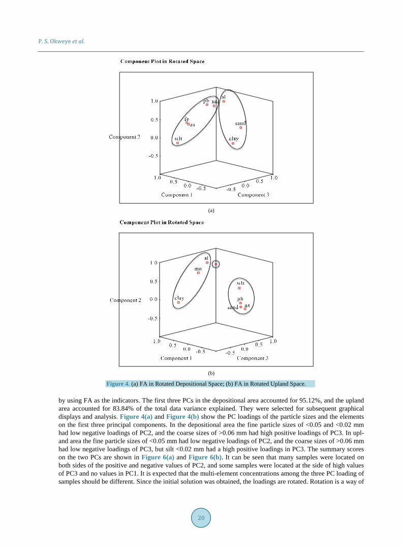
The component plot in rotated space shows the first three principal components (PCs) for the depositional area (Figure 4(a)), and the upland area (Figure 4(b)). The first three PCs may reveal a clearer explanation of the particle-size and element factor controlling the distribution and accumulation of the metals and particle sizes. The significant relationships between the particle-size variables and the elemental components were presented

Scree Plot

Component Number

87654321

Eige

nvalu

e

5

4

3

2

1

0

-1

(a)

Scree Plot

Component Number

87654321

Eige

nvalu

e

4

3

2

1

0

-1

(b)

Figure 3. (a) Scree Plot for the Depositional Area; (b) Scree Plot for the Upland Area.

P. S. Okweye et al.

20

(a)

(b)

Figure 4. (a) FA in Rotated Depositional Space; (b) FA in Rotated Upland Space. by using FA as the indicators. The first three PCs in the depositional area accounted for 95.12%, and the upland area accounted for 83.84% of the total data variance explained. They were selected for subsequent graphical displays and analysis. Figure 4(a) and Figure 4(b) show the PC loadings of the particle sizes and the elements on the first three principal components. In the depositional area the fine particle sizes of <0.05 and <0.02 mm had low negative loadings of PC2, and the coarse sizes of >0.06 mm had high positive loadings of PC3. In upl-and area the fine particle sizes of <0.05 mm had low negative loadings of PC2, and the coarse sizes of >0.06 mm had low negative loadings of PC3, but silt <0.02 mm had a high positive loadings in PC3. The summary scores on the two PCs are shown in Figure 6(a) and Figure 6(b). It can be seen that many samples were located on both sides of the positive and negative values of PC2, and some samples were located at the side of high values of PC3 and no values in PC1. It is expected that the multi-element concentrations among the three PC loading of samples should be different. Since the initial solution was obtained, the loadings are rotated. Rotation is a way of

P. S. Okweye et al.

21

maximizing high loadings and minimizing low loadings so that the simplest possible structure is achieved. For this study, oblique rotation was used because it derives factor loadings based on the assumption that the factors were correlated. This was the case for these measures (variables). The oblique rotation gave the correla-tion between the factors in addition to the loadings (See Table 10).

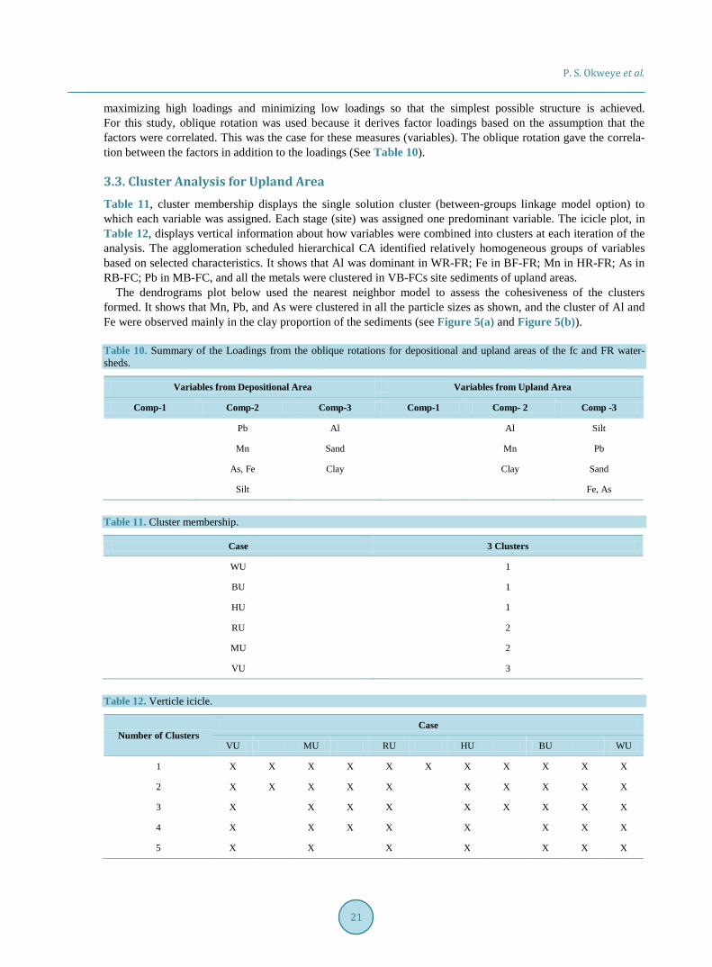
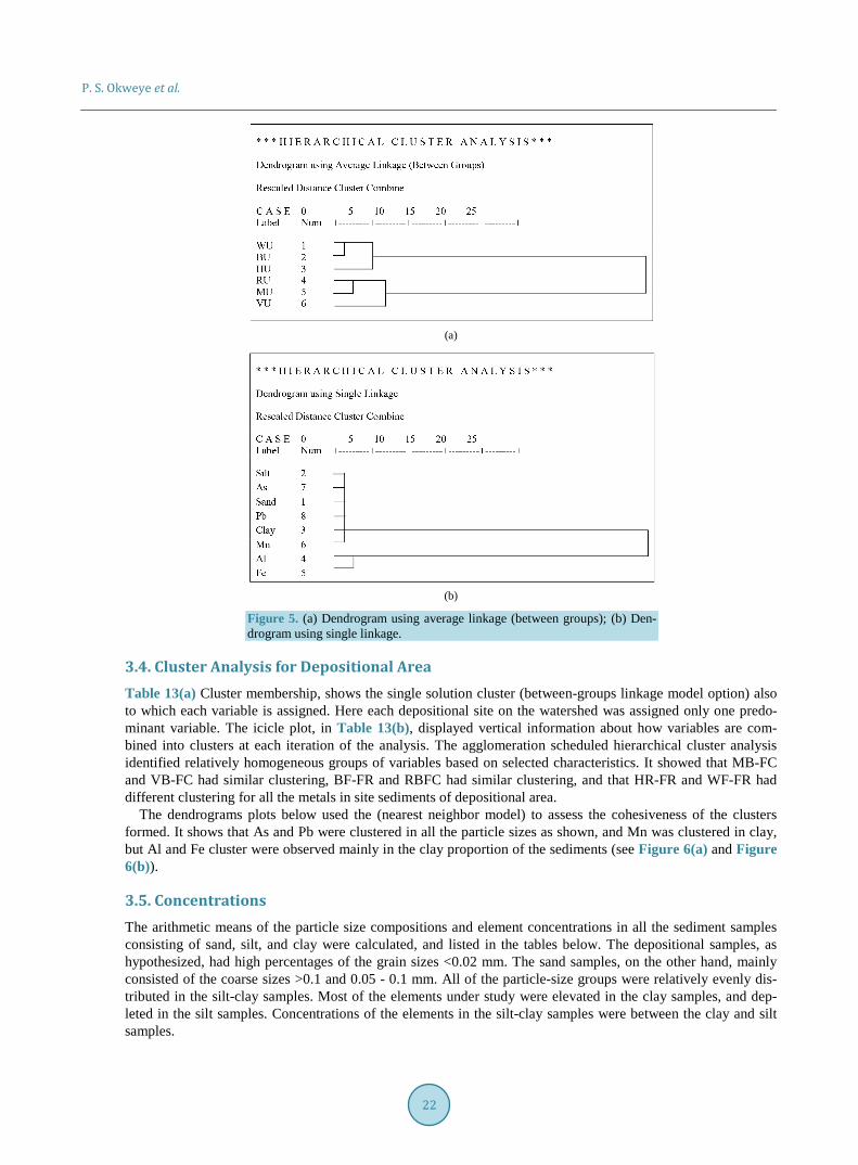
3.3. Cluster Analysis for Upland Area Table 11, cluster membership displays the single solution cluster (between-groups linkage model option) to which each variable was assigned. Each stage (site) was assigned one predominant variable. The icicle plot, in Table 12, displays vertical information about how variables were combined into clusters at each iteration of the analysis. The agglomeration scheduled hierarchical CA identified relatively homogeneous groups of variables based on selected characteristics. It shows that Al was dominant in WR-FR; Fe in BF-FR; Mn in HR-FR; As in RB-FC; Pb in MB-FC, and all the metals were clustered in VB-FCs site sediments of upland areas.

The dendrograms plot below used the nearest neighbor model to assess the cohesiveness of the clusters formed. It shows that Mn, Pb, and As were clustered in all the particle sizes as shown, and the cluster of Al and Fe were observed mainly in the clay proportion of the sediments (see Figure 5(a) and Figure 5(b)). Table 10. Summary of the Loadings from the oblique rotations for depositional and upland areas of the fc and FR water-sheds.

Variables from Depositional Area Variables from Upland Area

Comp-1 Comp-2 Comp-3 Comp-1 Comp- 2 Comp -3

Pb Al Al Silt

Mn Sand Mn Pb

As, Fe Clay Clay Sand

Silt Fe, As

Table 11. Cluster membership.

Case 3 Clusters

WU 1

BU 1

HU 1

RU 2

MU 2

VU 3

Table 12. Verticle icicle.

Number of Clusters Case

VU MU RU HU BU WU

1 X X X X X X X X X X X

2 X X X X X X X X X X

3 X X X X X X X X X

4 X X X X X X X X

5 X X X X X X X

P. S. Okweye et al.

22

(a)

(b)

Figure 5. (a) Dendrogram using average linkage (between groups); (b) Den- drogram using single linkage.

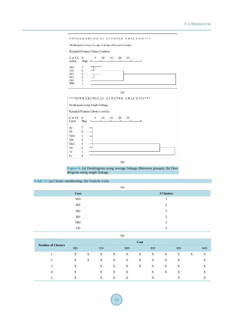
3.4. Cluster Analysis for Depositional Area Table 13(a) Cluster membership, shows the single solution cluster (between-groups linkage model option) also to which each variable is assigned. Here each depositional site on the watershed was assigned only one predo-minant variable. The icicle plot, in Table 13(b), displayed vertical information about how variables are com-bined into clusters at each iteration of the analysis. The agglomeration scheduled hierarchical cluster analysis identified relatively homogeneous groups of variables based on selected characteristics. It showed that MB-FC and VB-FC had similar clustering, BF-FR and RBFC had similar clustering, and that HR-FR and WF-FR had different clustering for all the metals in site sediments of depositional area.

The dendrograms plots below used the (nearest neighbor model) to assess the cohesiveness of the clusters formed. It shows that As and Pb were clustered in all the particle sizes as shown, and Mn was clustered in clay, but Al and Fe cluster were observed mainly in the clay proportion of the sediments (see Figure 6(a) and Figure 6(b)).

3.5. Concentrations The arithmetic means of the particle size compositions and element concentrations in all the sediment samples consisting of sand, silt, and clay were calculated, and listed in the tables below. The depositional samples, as hypothesized, had high percentages of the grain sizes <0.02 mm. The sand samples, on the other hand, mainly consisted of the coarse sizes >0.1 and 0.05 - 0.1 mm. All of the particle-size groups were relatively evenly dis-tributed in the silt-clay samples. Most of the elements under study were elevated in the clay samples, and dep-leted in the silt samples. Concentrations of the elements in the silt-clay samples were between the clay and silt samples.

P. S. Okweye et al.

23

(a)

(b)

Figure 6. (a) Dendrogram using average linkage (Between groups); (b) Den- drogram using single linkage.

Table 13. (a) Cluster membership; (b) Verticle icicle.

(a)

Case 3 Clusters

WD 1

BD 2

HD 3

RD 2

MD 2

VD 2

(b)

Number of Clusters Case

HD VD MD RD BD WD

1 X X X X X X X X X X X

2 X X X X X X X X X X

3 X X X X X X X X X

4 X X X X X X X X

5 X X X X X X X

P. S. Okweye et al.

24

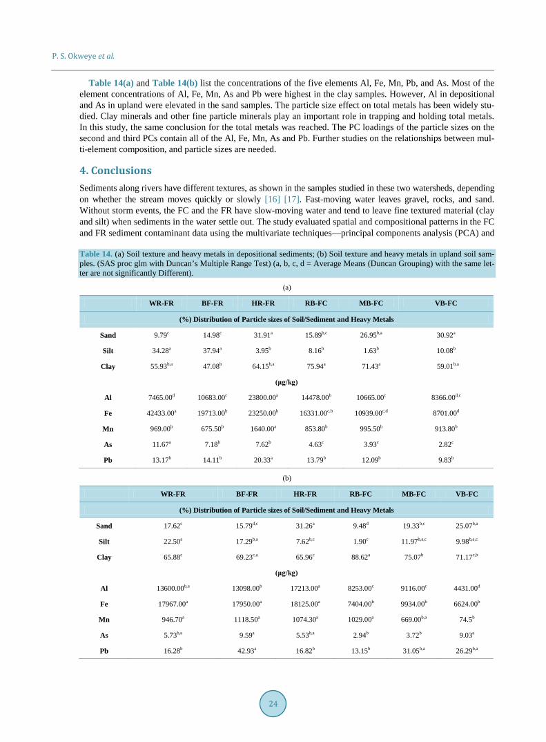
Table 14(a) and Table 14(b) list the concentrations of the five elements Al, Fe, Mn, Pb, and As. Most of the element concentrations of Al, Fe, Mn, As and Pb were highest in the clay samples. However, Al in depositional and As in upland were elevated in the sand samples. The particle size effect on total metals has been widely stu-died. Clay minerals and other fine particle minerals play an important role in trapping and holding total metals. In this study, the same conclusion for the total metals was reached. The PC loadings of the particle sizes on the second and third PCs contain all of the Al, Fe, Mn, As and Pb. Further studies on the relationships between mul-ti-element composition, and particle sizes are needed.

4. Conclusions Sediments along rivers have different textures, as shown in the samples studied in these two watersheds, depending on whether the stream moves quickly or slowly [16] [17]. Fast-moving water leaves gravel, rocks, and sand. Without storm events, the FC and the FR have slow-moving water and tend to leave fine textured material (clay and silt) when sediments in the water settle out. The study evaluated spatial and compositional patterns in the FC and FR sediment contaminant data using the multivariate techniques—principal components analysis (PCA) and Table 14. (a) Soil texture and heavy metals in depositional sediments; (b) Soil texture and heavy metals in upland soil sam-ples. (SAS proc glm with Duncan’s Multiple Range Test) (a, b, c, d = Average Means (Duncan Grouping) with the same let-ter are not significantly Different).

(a)

WR-FR BF-FR HR-FR RB-FC MB-FC VB-FC

(%) Distribution of Particle sizes of Soil/Sediment and Heavy Metals

Sand 9.79c 14.98c 31.91a 15.89b,c 26.95b,a 30.92a

Silt 34.28a 37.94a 3.95b 8.16b 1.63b 10.08b

Clay 55.93b,a 47.08b 64.15b,a 75.94a 71.43a 59.01b,a

(μg/kg)

Al 7465.00d 10683.00c 23800.00a 14478.00b 10665.00c 8366.00d,c

Fe 42433.00a 19713.00b 23250.00b 16331.00c,b 10939.00c,d 8701.00d

Mn 969.00b 675.50b 1640.00a 853.80b 995.50b 913.80b

As 11.67a 7.18b 7.62b 4.63c 3.93c 2.82c

Pb 13.17b 14.11b 20.33a 13.79b 12.09b 9.83b

(b)

WR-FR BF-FR HR-FR RB-FC MB-FC VB-FC

(%) Distribution of Particle sizes of Soil/Sediment and Heavy Metals

Sand 17.62c 15.79d,c 31.26a 9.48d 19.33b,c 25.07b,a

Silt 22.50a 17.29b,a 7.62b,c 1.90c 11.97b,a,c 9.98b,a,c

Clay 65.88c 69.23c,a 65.96c 88.62a 75.07b 71.17c,b

(μg/kg)

Al 13600.00b,a 13098.00b 17213.00a 8253.00c 9116.00c 4431.00d

Fe 17967.00a 17950.00a 18125.00a 7404.00b 9934.00b 6624.00b

Mn 946.70a 1118.50a 1074.30a 1029.00a 669.00b,a 74.5b

As 5.73b,a 9.59a 5.53b,a 2.94b 3.72b 9.03a

Pb 16.28b 42.93a 16.82b 13.15b 31.05b,a 26.29b,a

P. S. Okweye et al.

25

cluster analysis (CA). With the aid of PC and CA, the sediments from these watersheds were classified based on their texture into three fractions: sand, silt and clay. Significant differences were observed among the concentra-tions of the elements in the categories. Most of the elements detected were enriched in the fine-particle samples, where clay minerals were an important constituent [3]. On the other hand, elevated concentrations of Al and As were observed in the coarse (sand) samples. This may imply that the Al and As were present in the parent mate-rials that weathered to sand. PCA indicated association among all heavy metals determined in the environmental matrices (soil/sediment) analyzed, revealing that their high concentrations were due to the discharge of liquid wastes to the FC and FR watersheds. Interestingly, some of the wastewater from the Decatur plant enters the river untreated [18]. According to Gray [19], sewage treatment removes less than 100% of the metals from wastewater, so untreated wastewaters can be an important source of metals such as the ones analyzed in this study. Further, CA correlated all sampling sites impacted by contamination resulting from non-point sources, municipal wastes, sewages, and other sources. Metal concentrations from this study were higher than the USEPA’s MCL or background concentration values for Al, Fe, Mn, As and Pb. This indicated that there was metal pollution at all the sampling sites. Significant relationships from the Pearson’s correlation were also sup-ported by the results of the statistical methods (PCA and CA) used.

In summary, contaminants displayed distinct groupings (elements with similar properties) and spatial patterns; and relationships between particle size factors and chemical contaminant concentrations were explained in part with the multivariate statistical approaches. However, this multivariate statistical approach was as effective as simple correlation for this study, where contaminant concentrations were relatively high and correlation patterns were strong. In addition, the study refuted the null hypotheses. There was enough evidence from the overall re-sults of the study to support the theoretical notion that particle size distribution and sampling location influenced the level of heavy metal concentration within the watersheds. These results provide a framework for interpreting heavy metal distribution and sediment toxicity in biological communities at these watersheds.

Acknowledgements We would like to acknowledge Alabama A&M University Interdisciplinary Center for Health Sciences and Health Disparities in the College of Engineering, Technology and Physical Sciences with funding provided through the Evans-Allen Grant, administered by the College of Agricultural, Life and Natural Sciences (CALNS).

References [1] Greany, K.M. (2005) An Assessment of Heavy Metal Contamination in the Marine Sediments of Las Perlas Archipe-

lago, Gulf of Panama. Master of Science Thesis, Heriot-Watt University, Edinburgh. [2] Pekey, H.P., Karakas, S., Ayberk, L., Tolun, L. and Bakoglu, M. (2006) Ecological Risk Assessment Using Trace

Elements from Surface Sediments of Izmit Bay (Northeastern Marmara Sea) Turkey. Marine Pollution Bulletin, 48, 9-10, 946-953.

[3] Okweye, P., Tsegaye, T.D. and Garner. K.F. (2007) Distribution of Heavy Metals in Surface Water of the Wheeler Lake Basin in Northern Alabama. Journal of Environmental Monitoring and Restoration, 33, 91-100.

[4] Phillips, C.R. (2007) Bulletin of the Southern California Academy of Sciences, 106, 163-178, E Article 1. [5] Okweye, P. and Garner, K.F. (2009) Sediment Sampler (Patent Pending). [6] United Nations Environment Program and the World Health Organization (1996) Sediment Measurements. Water

Quality Monitoring—A Practical Guide to the Design and Implementation of Freshwater Quality Studies and Moni-toring Programs Edited by Jamie Bartram and Richard Balance.

[7] U.S. Environmental Agency (USEPA) (1994) 822-R-94-001. Drinking Water Regulations and Health Advisories. EPA’s Toxics Release Inventory, 1-3.

[8] Date, A.R. and Gray, A.L. (1989) Applications of Inductively Coupled Plasma Source Mass Spectrometry: Blackie, Glasgow.

[9] Platzner, I.T. (1997) Modern Isotope Ratio Mass Spectrometry. Chemical Analysis, 145, 187-189. [10] Kennett, D.J., Neff, H., Glascock, M.D. and Mason, A.Z. (2001) A Geochemical Revolution: Inductively Coupled

Plasma Mass Spectrometry. The Archaeological Record, 1, 22-26. [11] Grimm, L.G. and Yarnold, P.R. (2000) Introduction to Multivariate Statistics. In: Grimm, L.G. and Yarnold, P.R., Eds.,

Reading and Understanding More Multivariate Statistics, American Psychological Association, Washington DC, 3-21.

P. S. Okweye et al.

26

[12] SCB (2007) Bulletin of the Southern California Academy of Sciences, 106, 163-178, E Article 1. [13] Phillips, C.R. (2007) Bulletin of the Southern California Academy of Sciences, 106, 163-178, E Article 1. [14] Hatcher, L. (1994) A Step-by-Step Approach to Using the SAS® System for Factor Analysis and Structural Equation

Modeling. SAS Institute Inc, Cary. [15] Cattell, R.B. (1966) The Scree Test for the Number of Factors. Multivariate Behavioral Research, 1, 245-276.

http://dx.doi.org/10.1207/s15327906mbr0102_10 [16] Alagarsamy, R. (2006) Distribution and Seasonal Variation of Trace Metals in Surface Sediments of the Mandovi Est-

uary West Coast of India. Estuarine, Coastal and Shelf Science, 67, 333-339. http://dx.doi.org/10.1016/j.ecss.2005.11.023

[17] Jonathan, M.P., Ram-Mohan, V. and Srinivasalu, S. (2004) Geochemical Variations of Major and Trace Elements in Recent Sediments, off the Gulf of Mannar, Southeast Coast of India. Environmental Geology, 45, 466-480. http://dx.doi.org/10.1007/s00254-003-0898-7

[18] (2008) ADEM Files Suit against Hanceville Water Board. Huntsville Times, 15 June 2008, p. A20. [19] Gray, D. (2004) Doing Research in the Real World. SAGE Publications, Various Paginations.