Factors Affecting Magnetic Flux Leakage Inspection of Tailor-Welded Blanks A Montgomery1, P Wild2, L Clapham3

1Department of Mechanical Engineering, Queen’s University, McLaughlin Hall, Queen’s University, Kingston, Ontario, Canada K7L 3N6 2Department of Mechanical Engineering, University of Victoria, P.O. Box 3055, STN CSC, Victoria, British Columbia, Canada V8W 3P6 3Department of Physics, Queen’s University, Stirling Hall, Queen’s University, Kingston, Ontario Canada K7L 3N6 Corresponding Author: P. Wild, e-mail - pwild@uvic.ca. MFL Inspection of Tailor-Welded Blanks

Abstract

The development of a laboratory-based tailor-welded blank (TWB) inspection system

using the principles of magnetic flux leakage (MFL) is presented. The effects of variations in

inspection system operating parameters are quantified to allow for optimized system

performance. The parameters examined included the applied magnetic field strength, inspection

scanning velocity, spatial resolution of acquired signals, specimen end effects, and pole-piece

lift-off. The results indicate that this inspection method is relatively insensitive to operating

parameters and is, therefore, robust.

List of Notation

samplef Sampling frequency

refMFL Magnitude of signal at reference speed

ppMFL Magnitude of signal

SR Spatial resolution

scanV Scanning velocity

SigRd% Percentage signal reduction

2

1.0 Introduction

1.1 Tailor-Welded Blanks

In the automotive industry, car body-parts are formed from pieces of sheet metal known as

‘blanks’. Conventional blanks are typically uniform in thickness, surface finish and formability.

A tailor-welded blank (TWB) is composed of two or more pieces, each having its own

properties, laser-welded to form a single blank. TWBs enable the ‘tailoring’ of the blank design

to meet specific requirements [1]. For example, in the fabrication of a door inner panel, heavy-

gauge material can be used adjacent to the load bearing hinges while lighter-gauge material can

be located in the area away from the hinges. This results in reduced part weight, reduced vehicle

weight and increased fuel efficiency. In 2001, the automotive industry produced 28.8 million

TWB units. This number is expected to rise to 90 million units by 2005 [2].

The quality of the weld in a TWB is critical to successful part forming operations. The

International Standards Organization (ISO) [3] and the Auto/Steel Partnership (ASP) [1] have

developed acceptance guidelines to evaluate the quality of the weld in a TWB. A variety of non-

destructive inspection methods have emerged to monitor TWB weld quality as defined by the

ISO and ASP guidelines. However, limitations of these methods have prevented widespread

adoption of a single preferred method while some manufacturers continue to rely on visual

inspection by operators. For a detailed review of these inspection methods the reader is referred

to Gartner, Sun, and Kannatey-Asibu [4] and O’Connor, Clapham, and Wild [5]. Gartner et al.

provide a detailed review of in-process techniques while more emphasis is placed on post-

process techniques in O’Connor et al.

3

1.2 Magnetic Flux Leakage Inspection

MFL inspection has been used extensively and with great success in the pipeline industry for

the past 30 years [6]. During this period, numerous experiments have also been done to develop

theoretical models and more recently, finite element models. These models have been used to

predict the magnetic flux leakage field from defects in a pipe wall within certain constrains. For

a review of relevant MFL theory and experiments, the reader is referred to Mandache and

Clapham [7].

In general, when a magnetic field is applied to a ferromagnetic specimen, magnetic flux

passes through the material. The flux density is determined by the strength of the applied field

and the permeability of the material. In the MFL inspection technique, specimens are

magnetized to saturation which is the maximum magnetic flux capacity of a material based on its

permeability. Metal loss defects result in a localized reduction in the cross-sectional area of the

material. This forces some of the flux to ‘leak’ into the surrounding air, where it is detected by a

coil or a Hall effect sensor. Signal analysis is used to relate the leakage signal to the

characteristics of the defects.

In 2000, a feasibility study concerning the application of the MFL inspection technique to the

evaluation of TWB weld quality was conducted by O’Connor et al. [5]. The study used a

rudimentary MFL system to generate and record MFL data from artificial pinholes drilled into

the welds of TWBs. The results demonstrated that pinhole defects as small as 0.34 mm in

diameter could be detected and a relationship between the magnitude of the defect and the MFL

signal was established. In a later study, it was shown that MFL is able to detect naturally

occurring weld defects such as pinholes, mismatch, missed welds, lack of fusion and porosity

4

[8]. This work confirmed that MFL has excellent potential as a practical inspection method for

welds in TWBs.

Based on the positive findings of the feasibility study, a new MFL inspection system for an

industrial application was developed. Using this system, the effects of operating parameters on

the MFL signals were investigated. Operating parameters that were examined include: applied

field strength, scanning velocity, sampling resolution, pole piece lift-off, and proximity to

specimen edges. This paper describes the features of the newly developed inspection system and

the results of the operating parameter studies.

2.0 Experimental Methods

2.1 Apparatus

The design of the magnetic circuit and inspection system were based on the rudimentary

system used by O’Connor et al. [5]. As shown in Figure 1, the magnetic circuit consists of four

Nd-Fe-B permanent magnets (1 cm x 2 cm x 4 cm) placed in a row along the upper center of the

assembly. Coupled to the magnets are soft iron blocks in a horseshoe configuration, which direct

the magnetic flux down to the specimen. The TWB specimen closes the magnetic circuit with its

weld lying transverse to the flux direction. A Hall sensor (Honeywell SS94A1) is used to

measure the radial component of the MFL signal. This sensor is supported on the Hall sensor

mounting assembly, as shown in Figure 2, which provides spring loading of the sensor against

the flat (i.e. non-stepped) surface of the TWB. The pole pieces of the magnet assembly (the soft

iron blocks in contact with the TWB specimen) are mounted on wheels. Wheel diameter and

position are such that a small gap exists between the pole pieces and the surface of the specimen.

Flux density variation is achieved with a backing circuit using a large soft iron plate attached to

5

the top of the magnet assembly. The plate is hinged on one side and attached to a threaded rod

(or screw) on the other. By turning the screw, the position of the plate relative to the magnet

assembly is adjusted. The flux level in the magnetic circuit is monitored with a Hall sensor

(F.W. Bell BH-700) embedded in an aluminum sheet located between the pole pieces. A

photograph of inspection system is shown in Figure 2.

TWB specimens are aligned with and then clamped to a table which is attached to a linear

positioning system driven by a stepper motor, as shown in Figure 3. The TWB is located by

aligning the weld line with a longitudinal and centred guideline on the surface of the table. Table

motion is controlled via command level language with a PC and a motor controller. The position

of the table is recorded using a rotary encoder on the stepper motor shaft. A National

Instruments 6023E data acquisition card is used for data logging for the rotary encoder and Hall

sensor. The Hall effect sensor output, prior to data logging, is filtered using a low pass filter

with a cutoff frequency of 1000 Hz to remove unwanted high frequency noise.

Figure 3 also illustrates specimen orientation and motion. The thin side of the specimen is

placed on the positive y-axis side with the front edge of the specimen aligned at the home

position. Typically, the weld, excluding the heat affected zone, is between 0.5 mm and 1.0 mm

in width. Scanning begins with the blank in the home position. The first scan is taken by

moving the blank in the positive x-direction along the entire length of the weld. The Hall effect

sensor is then translated 0.25 mm in the positive y-direction, and the scan is repeated along the

entire length of the weld. These scans are repeated until the full width of the weld has been

scanned. MFL profiles of the weld line are generated by compiling data from these scans.

A typical profile resulting from a scan of a weld in a TWB is shown in Figure 4. The defect

profile shown in the figure is for a pinhole defect and is characterized by a broad peak. This

6

peak is usually centered over the weld defect. The length of the peak is dependent on the length

of the defect and the amplitude of the signal is dependent on the depth and width of the defect.

Further discussion of MFL profiles for various weld defects can be found in Montgomery et al

[8].

2.2 Signal Conditioning

To analyze the collected MFL data, the raw signals were digitally filtered using a second

order Bessel bandpass filter with corner frequencies of 0.5 cycles/mm and 5 cycles/mm. This

process, commonly know as ‘detrending’, removed the DC component of the signal and the low

frequency background. In addition, unwanted high frequency noise was eliminated. The 0.5

cycles/mm corner frequency was derived by trial and error while monitoring the signal for

distortion. The 5 cycles/mm corner frequency was derived from the Nyquist Theorem that states

that the maximum frequency that can be detected in a signal without aliasing is half of the

sampling resolution (10 cycles/mm – a result from Section 3.3). To calculate the peak-to-peak

value of the defect signal, the scan line from the profile with the largest peak-to-peak value was

used (referred to as the peak scan line). Peak-to-peak values were determined after the acquired

data had been filtered. Details of the signal processing techniques are discussed in Montgomery

et al [9]

2.3 Specimens

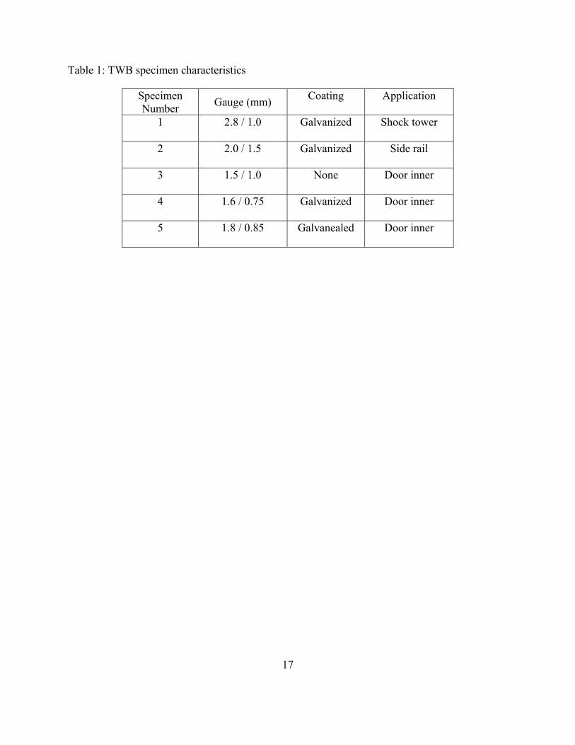
A commercial TWB manufacturer provided five specimens for the experiments. The TWBs

were welded with an 8 kW CO2 laser and all specimens were cold-rolled carbon steel. Specimen

specifications are summarized in Table 1. The two values in the “gauge” column of Table 1

refer to the thickness of the pieces of sheet metal comprising the TWB. As received from the

manufacturer, these specimens contained defect-free welds. Subsequently, one 0.5 mm diameter

7

pinhole was drilled through the full thickness of the estimated center of the weld line in each

specimen. These pinholes, which are similar in size to naturally occurring pinhole defects, act as

reference “defects” in this study.

3.0 Sensitivity Studies

There are a number of parameters that can affect the MFL signal for a given defect. In

Sections 3.1 to 3.5, the results of five studies are presented in which the sensitivities of MFL

inspection to the following parameters were assessed: applied field strength, scanning velocity,

signal resolution, specimen end effects, and pole-piece lift-off.

3.1 Applied Field Strength

The effect of applied magnetic field strength on the MFL defect signal is an important issue.

Jansen et al. [10] demonstrated that a high magnetization level is the key factor in

characterization of defects in pipelines. The purpose of the current study was to determine the

relationship between the applied magnetic field strength and MFL signals from a defect in a

TWB weld. The range of magnetic field strength in these experiments was determined by the

range of the adjustable backing circuit and the permanent magnets. This was measured to be

0.27 Tesla to 0.45 Tesla in the pole piece. These values typically produce magnetic saturation in

the blank. Results of a further study investigating a much lower range of flux densities has been

published elsewhere [11].

In the first stage of the study, the shape of the MFL signal profile as a function of applied

field strength was examined. The scans were conducted at 200 mm/s and with a spatial

resolution of 40 samples/mm. Plots of the MFL profiles for specimen 5 at the highest and lowest

8

applied field strength are shown in Figure 5. Although the extent of the defect in the X and Y

directions is similar in both cases, the peak amplitude increases with increasing flux density,

since at higher sample flux densities more flux will be forced into the air above the pinhole.

These profiles are representative of all the profiles obtained for all of the blanks in this study.

In the second stage of the study, scans were conducted on each specimen for a range of flux

densities. Flux densities were measured using the embedded Hall effect sensor with the magnet

assembly located at mid-span of the specimen. The scans were conducted at 200 mm/s with a

spatial resolution of 40 samples/mm. For each specimen type, the peak-to-peak value of the

defect signal from the artificial defect was measured. The flux density in the pole-piece was

calculated using the readings from the embedded Hall sensor. Shown in Figure 6 are the results

for specimens 2 and 5, which were representative of the results for all specimens. The results

indicate a monotonically increasing trend in the peak-to-peak values as a function of applied

field strength. This is consistent with the results shown in Figure 5 and also with the

explanation that at higher flux densities more flux is expected to be forced into the air in the

defect vicinity. Specimen 1 is thinner and therefore will be more highly saturated than specimen

2, hence the larger overall MFL signal.

The difference in magnitude of the peak-to-peak values for the different specimen types is

ascribed to differences in the thickness ratios (i.e. ratio of thicknesses of the two sheets of which

the TWB is comprised) of the specimens. As the thickness ratio increased, the peak-to-peak

value of the defect signal for the artificial defect increased.

It was also determined that for each specimen type, although there was an increase in the

peak-to-peak value of the defect signal with applied field strength, there was no significant

change in the signal-to-noise ratios of the defect signal [10]. In the context of MFL, noise refers

not to electromagnetic noise but to the small, reproducible variation in the signal due to material

variations. These results are consistent with the finding of a numerical study by Altschuler et al.

in which it was shown that signal-to-noise ratios for MFL signals from pipeline defects were

relatively insensitive to the strength of the applied field [12].

3.2 Scanning Velocity

Relative motion between the magnetic field and the magnetized material induces eddy

currents in the magnetized material. These eddy currents generate an opposing magnetic field

that reduces the amount of flux and, thereby, the overall applied field in the sample. In the

pipeline industry, where inspection speeds reach 8 m/s, the reduction in MFL signals can be as

much as 75% [13]. In the TWB manufacturing process, welding and inspection speeds are much

lower (typically 150 mm/s) and the geometry (flat plate as opposed to a cylinder) does not

encourage significant opposing eddy current fields. The purpose of this study was to determine

the effect of scanning velocity on the MFL signals at typical TWB scanning speeds.

All five specimen types were used for this study. The flux density in the pole pieces and the

spatial resolution were held constant at 0.41 Tesla and 40 samples/mm, respectively. The scan

velocity was set to 1 mm/s and a multi-pass scan of the of the weld was taken.. The scan was

then repeated at the following velocities (mm/s): 10, 20, 30, 40, 50, 60, 70, 80, 90, 100, 120, 140,

160, 180, and 200. Signals were examined as a function of velocity, with particular attention to

signal reduction. Signal reduction was calculated using the following equation:

( ){ } 100*% refppref MFLMFLMFLSigRd −= [1]

where %SigRd is the percentage of signal reduction; MFLref is the peak-to-peak value of the

defect signal at 1 mm/s; and MFLpp is the peak-to-peak value of the defect signal at a given 9

velocity. MFLref was set to 1 mm/s as this was the slowest speed at which the postioning table

could be operated. Note that, “peak-to-peak value”, refers to the difference between the adjacent

positive and negative peaks which are typical of a pin-hole defect, as shown in Figure 5.

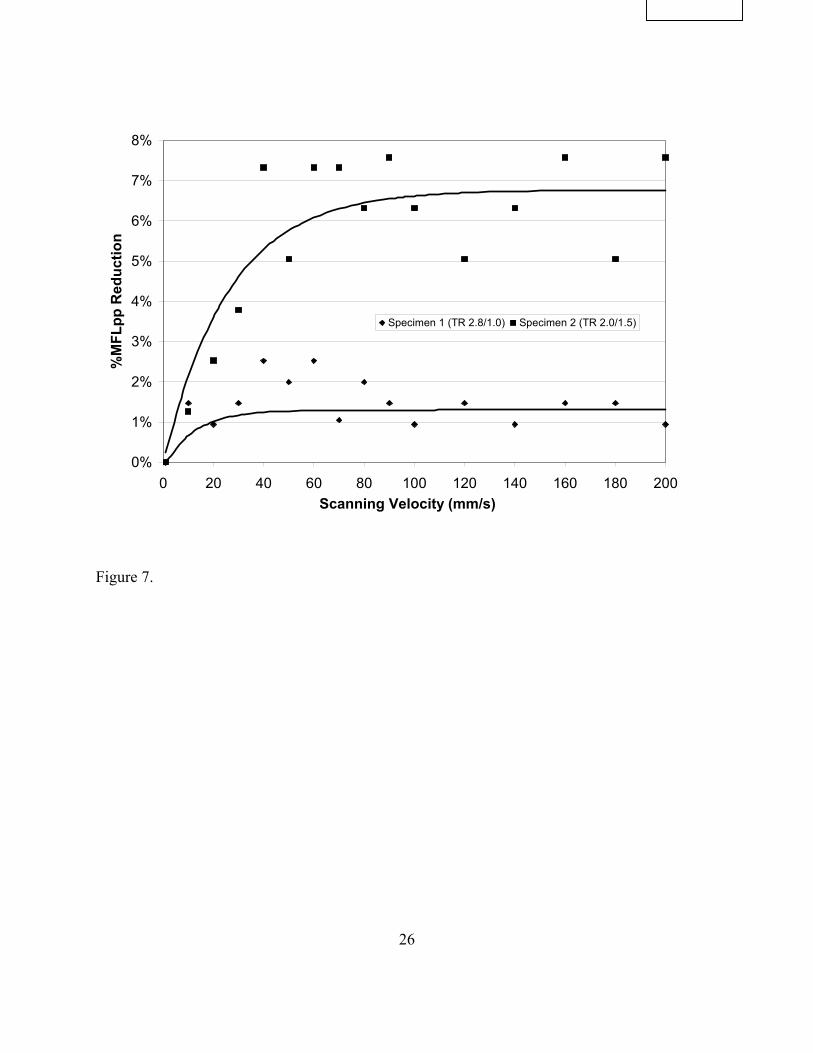
Figure 7 shows the results for specimens 1 and 2, which are representative of the range of

signal reduction that occurred in all specimens. Specimens 1 and 5 showed little or no signal

reduction as scanning velocity increased. Specimens 2, 3, and 4 showed reductions of up to 8%.

Typically, the majority of the velocity effects occurred below 80 mm/s and the shape of the MFL

signals was insensitive to velocity. As expected, the measured signal reductions due to velocity

are much smaller than those found in pipelines by Atherton et al. [13] since greater reductions

are expected for defects in thicker materials.

3.3 Signal Spatial Resolution

In MFL inspection of pipelines, sampling of MFL signals is usually performed at a fixed

spatial resolution rather than at a fixed temporal resolution because the speed of the inspection

tool can vary [14]. Having a high-resolution system increases the amount of data acquired,

which in turn increases the ability to characterize defects. However, system designs must

optimize the trade-off between increased resolution and superfluous data [15]. The purpose of

this study was to find a range of spatial resolutions that maximized signal quality while

minimizing the amount of data collected, stored, and analyzed. Spatial resolution was calculated

by using the following formula:

scan

sample

Vf

SR = [2]

10

11

where SR is spatial resolution [samples/mm]; Vscan is the scanning velocity [mm/s]; and fsample is

the sampling frequency of the data acquisition system [samples/s]

All five specimens were used for this study. MFL signals were analyzed in the spatial

frequency domain using the FFT (Fast Fourier Transform) technique. In the spatial frequency

domain, the frequency is determined with respect to the position rather than time. Shown in

Figure 8 is a spectral plot of a highly over-sampled MFL signal (spatial resolution of 40

samples/mm). This plot is representative of the signals for all of the specimens. The largest

frequency components of the MFL signal occur at less than 1 cycle/mm. Based on the Nyquist

sampling theorem, to avoid aliasing, the sampling frequency should, therefore, be at least 2

sample/mm. However, to ensure that a quality high-resolution MFL signal a factor of safety of 5

was applied and sampling was done at 10 samples/mm. Based on the results of this work, the

data acquisition program was modified so that the spatial resolution of the signal was maintained

at 10 samples/mm for any scanning velocity.

3.4 End Effects

The purpose of this investigation was to assess the effect of the proximity of a defect to the

edge of the TWB. Possible changes in flux density as the pole pieces move off the end of the

specimen were also examined.

Specimen 1 was scanned for the full length of the weld line (scan velocity: 200 mm/s, spatial

resolution: 10 cycles/mm, pole piece flux density: 0.410 Tesla) after two 1.1 mm diameter holes

were drilled in the weld line, 3 mm and 100 mm from the end of the specimen. In this test, the

Hall sensor was allowed to run off the end of the specimen onto a small square piece of plate

glass, flush with the end of the specimen.

12

Figure 9 shows the MFL data for this scan of specimen 1. Peaks for the 1.1 mm holes are

clearly visible. The large spike in the signal at approximately 380 mm is due to the movement of

the Hall sensor off of the end of the specimen. The signal from the 1.1 mm hole closest to the

edge is reduced compared to the signal from the 1.1 mm hole 100 mm away from the edge.

This reduced signal from the hole close to the specimen edge is caused by the decreased flux

applied to the specimen as a portion of the magnet assembly rolls off the specimen. Although

edge effects will not affect the ability to detect defects, they must be considered when making

defect size estimations based on the defect signal if the defect is close to the edge of the

specimen.

3.5 Pole Piece Lift-off

It is important in automotive applications that the scanning process does not mark the surface

of the TWB. The effect of increasing the distance between the specimen and the magnet pole

pieces to reduce the potential of damaging contact was, therefore, investigated. Pole-piece lift-

off was accomplished using wheels that provided a specified clearance from the TWB surface.

Consideration was given to the level of applied field as the lift-off between the specimen and the

pole pieces increased. This study examined the effect of lift-off distances from three sets of

wheels giving three gap distances: 0.25 mm, 0.5 mm and 1.13 mm.

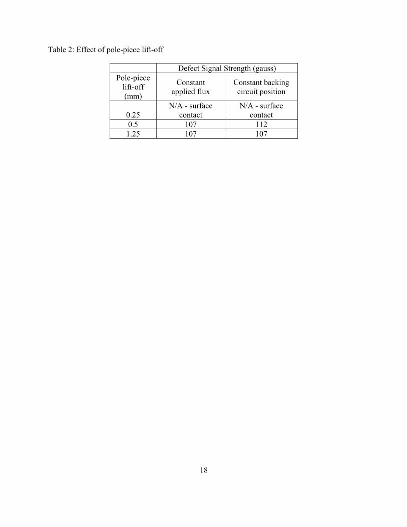
MFL data was collected using specimen 5 for each set of wheels under two circumstances:

(1) The flux in the pole pieces was maintained constant at 0.410 Tesla by adjusting the backing

circuit position for each set of wheels. (2) The backing circuit position was held constant while

the wheel sets were changed. For both methods, the peak-to-peak value of the defect signal was

13

determined and compared for each wheel set. The scanning velocity was 200 mm/s and the

spatial resolution of the acquired signals was 10 samples/mm.

The results of the lift-off tests are summarized in Table 2. For the tests at constant flux, the

changes in peak-to-peak values were insignificant for lift-offs of 0.50 mm and 1.13 mm. In both

cases, MFL peak-to-peak values were calculated to be 107 gauss. The lift-off of 0.25 mm

resulted in contact between the TWB and the pole pieces and this data was, therefore,

disregarded. For the case where the backing circuit position setting was held constant,

decreasing the lift-off distance from 1.13 mm to 0.5 mm caused an increase in the peak-to-peak

value of the defect signal of 4.7%.

Based on the results of this study, the 0.50 mm lift off wheel set was chosen for the MFL

inspection system in this application. It provided increased magnetization from the 1.13 mm

wheel set but did not mark the specimen like the 0.25 mm wheel set.

4.0 Conclusions

The MFL inspection method had been shown to be relatively insensitive to variations in

operating parameters over the ranges studied. Peak-to-peak defect signals increase as the applied

field strength increases but signal-to-noise ratios are relatively unaffected. The effect of

scanning velocity on MFL signals was less than 8% over a wide range of velocities. Between 80

mm/s to 200 mm/s the incremental reduction in the signal was less than 1%. The sampling

resolution study determined that the components of interest occur at spatial frequencies of less

than 1 cycle/mm, a resolution that is easily achieved at typical welding speed using even the

14

most basic of data acquisition equipment. The pole piece lift-off study found that proper

magnetization of the specimen could be maintained with a gap which is large enough that contact

between the pole pieces and the specimen does not occur. Lastly, defects were detected over the

full length of the weld seam, although signal magnitude decreases at the edges of the blank. In

conclusion, this study has shown that MFL inspection of TWBs is a robust method which is not

adversely influenced by small variations in the inspection process parameters.

15

References

[1] Auto/Steel Partnership, Tailor Welded Blank Acceptance Guidelines, Southfield,

Michigan, (1996).

[2] T. Bagsarian,, New Steel Magazine, (2000).

http://www.newsteel.com/2000/NS0005f1.htm

[3] International Standard, ISO 13919-1, Welding – Electron and Laser-Beam Welded Joints

– Guidance on Quality Levels for Imperfections – Part 1:Steel, Switzerland, (1996).

[4] M. Gartner, A. Sun, and E. Kannatey-Asibu, Journal of Laser Applications, 11(4):153

(1999).

[5] S. O’Connor, L. Clapham, and P. Wild, Measurement and Science Technology, Institute

of Physics Publishing, 13:157 (2002).

[6] H. Haines, et al., Pipe Line & Gas Industry, 82(3):49 (1999).

[7] C. Mandache and L. Clapham, Journal of Physics D: Applied Physics, 36 (20):2427

(2003).

[8] A. Montgomery, P. Wild, and L. Clapham, The British Institute of Non-Destructive

Testing, 46(5):260 (2004).

[9] A. Montgomery, M. Sc. Thesis, Queen’s University (2003).

[10] H.J.M Jansen, P.B.J. van de Camp, and M. Geerdink, INSIGHT, British Journal for NDT,

36(9):672 (1994).

[11] P. Hook, L. Clapham, and P.Wild, submitted to INSIGHT, British Journal for NDT

(2006).

[12] E. Altschuler, and A. Pignotti, NDT&E International, 28(1):35 (1995).

[13] D.L.,Atherton, C Jagadish, P. Laursen, V. Storm, F. Ham, and B. Scharfenberger, Oil and

Gas Journal, 88:84 (1990).

[14] D.L. Atherton and E. Quek, Canadian Electrical Engineering Journal, 13(1):27 (1998).

16

[15] J.B., Nestleroth, and T.A. Bubenik. The Gas Research Institute, (1999).

http://www.battelle.org/pipetechnology/MFL/MFL98Main.html

17

Table 1: TWB specimen characteristics

Specimen Number Gauge (mm) Coating Application

1 2.8 / 1.0 Galvanized Shock tower

2 2.0 / 1.5 Galvanized Side rail

3 1.5 / 1.0 None Door inner

4 1.6 / 0.75 Galvanized Door inner

5 1.8 / 0.85 Galvanealed Door inner

18

Table 2: Effect of pole-piece lift-off

Defect Signal Strength (gauss) Pole-piece

lift-off (mm)

Constant applied flux

Constant backing circuit position

0.25 N/A - surface

contact N/A - surface

contact 0.5 107 112

1.25 107 107

19

List of Figure Captions

Figure 1 - Schematic drawing of magnet assembly.

Figure 2 – Photograph of MFL test rig.

Figure 3 – Schematic drawing of MFL test rig (DAQ = Data Acquisition Equipment)

Figure 4 – MFL profile for a typical weld line showing a defect.

Figure 5 - MFL profiles for specimen 5 at the highest (0.45 T) and lowest (0.27 T) applied field

strengths measured in the pole pieces.

Figure 6. The peak-to-peak defect signal versus applied field strength for specimens 2 and 5

(Note: TR is Thickness Ratio).

Figure 7 - Peak-to-peak signal reduction as a function of scanning velocity for specimens 1 and

2.

Figure 8 – Spectrum of MFL signal.

Figure 9 - MFL data with 1.1 mm defects at 100 mm and 3 mm from the end of the specimen.

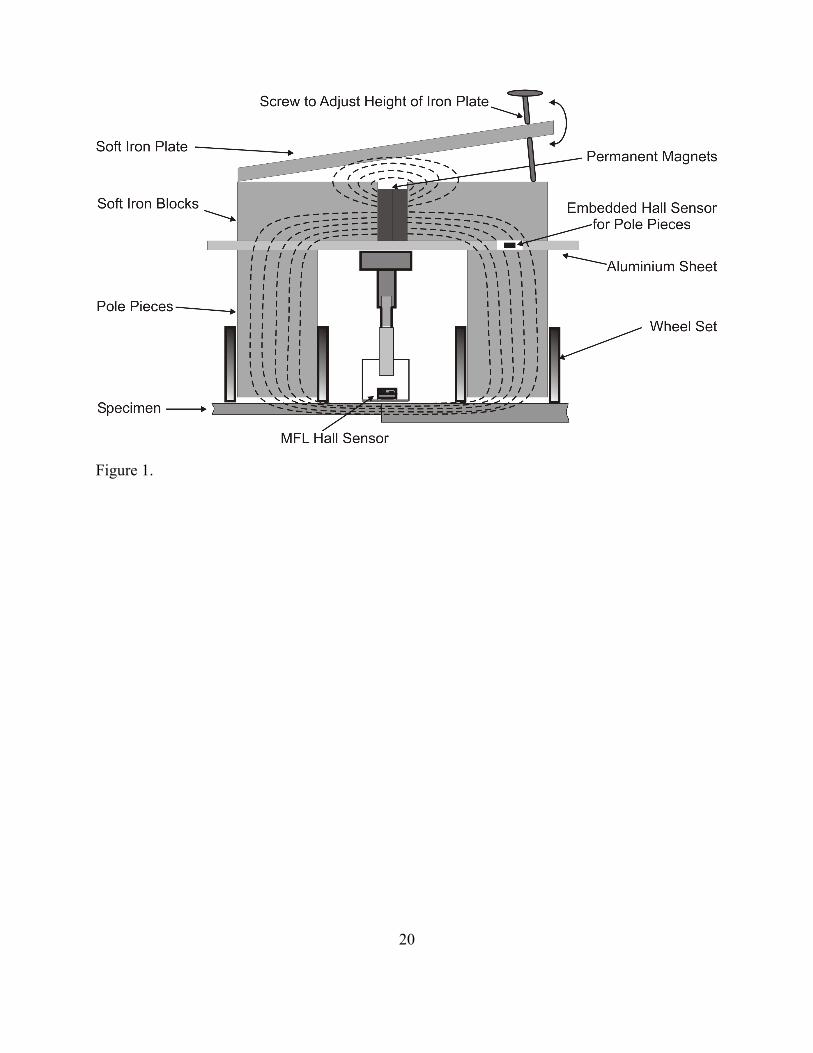
Figure 1.

20

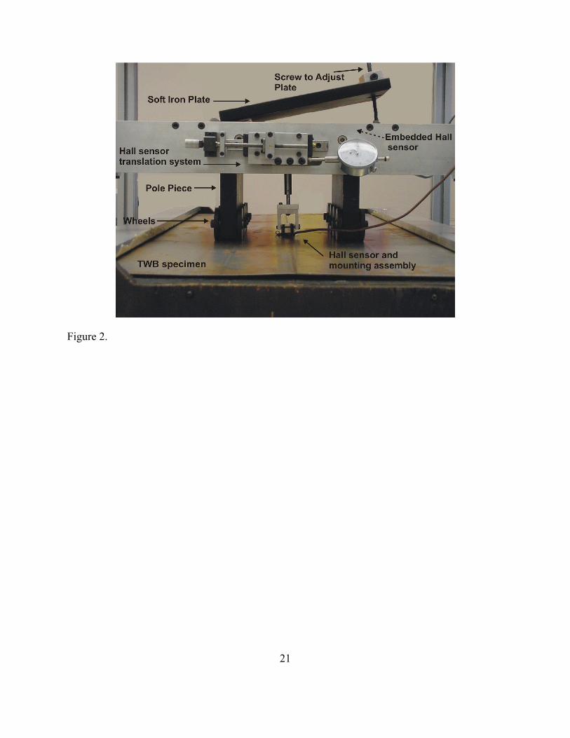
Figure 2.

21

Figure 3.

22

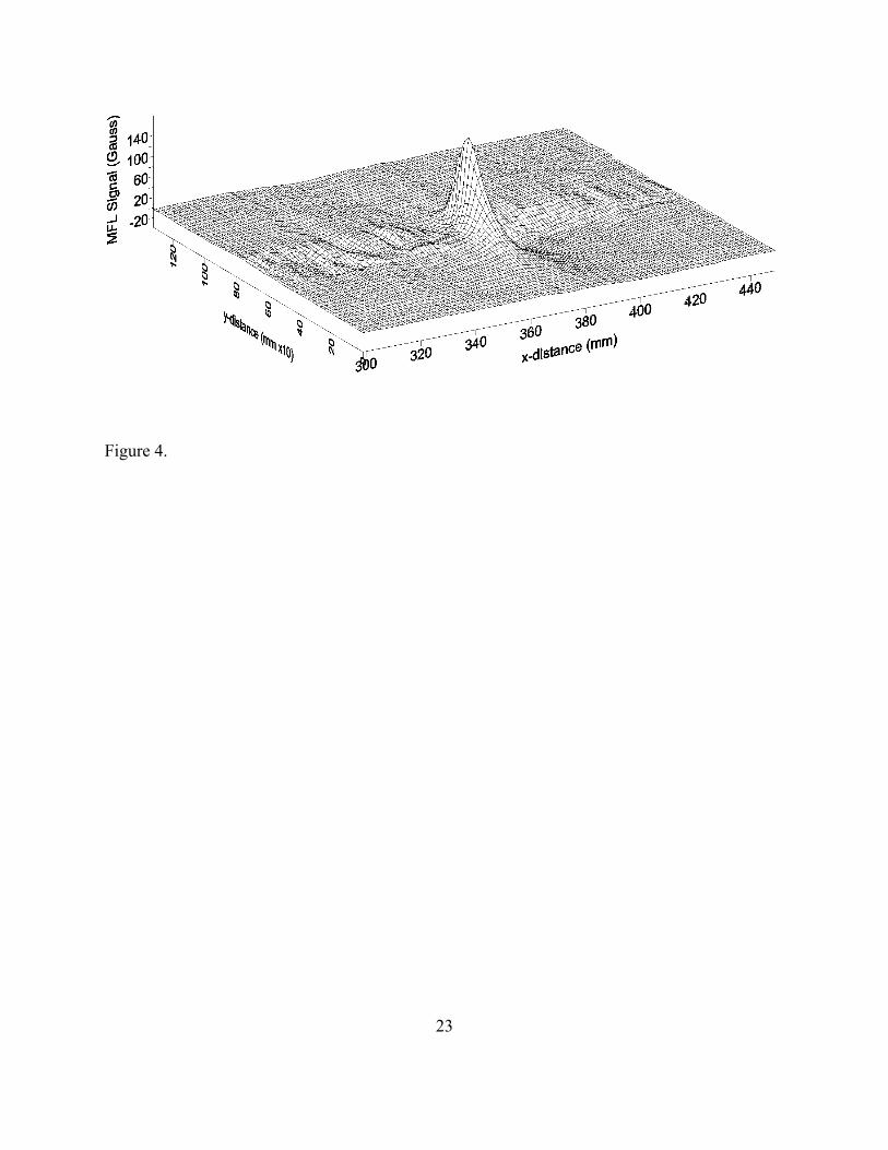
Figure 4.

23

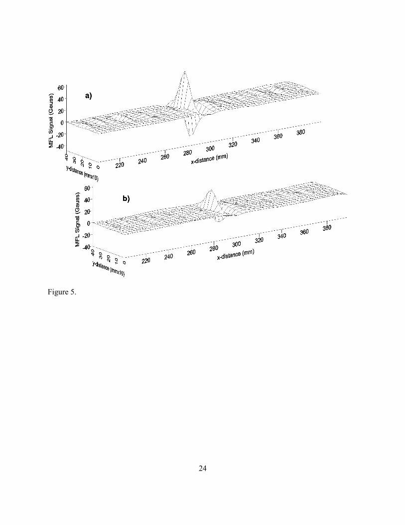
Figure 5.

24

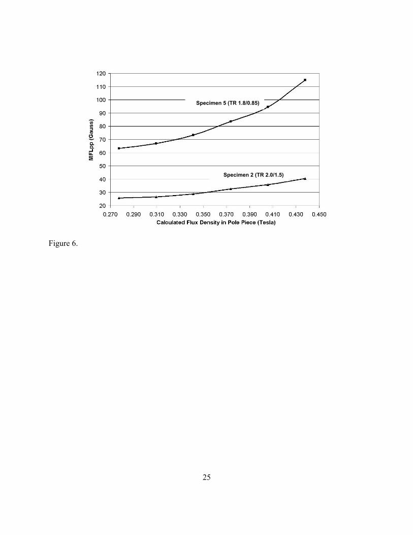
Specimen 5 (TR 1.8/0.85)

Specimen 2 (TR 2.0/1.5)

Figure 6.

25

0%

1%

2%

3%

4%

5%

6%

7%

8%

0 20 40 60 80 100 120 140 160 180 200Scanning Velocity (mm/s)

%M

FLpp

Red

uctio

n

Specimen 1 (TR 2.8/1.0) Specimen 2 (TR 2.0/1.5)

Figure 7.

26

Figure 8.

27

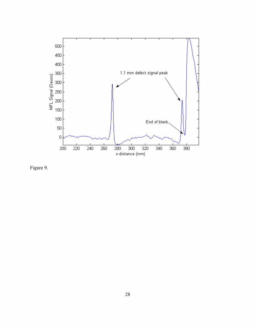
Figure 9.

28

29

Acknowledgements

The authors would like to thank the Centre for Automotive Materials and Manufacturing

(CAMM) in Kingston, Ontario for providing funding for this research.