Factors Affecting Money Supply (M0) in the Economyeuacademic.org/UploadArticle/1737.pdfsituations that hinders economic growth. The researchers look into the best model in order to

3268

ISSN 2286-4822

www.euacademic.org

EUROPEAN ACADEMIC RESEARCH

Vol. III, Issue 3/ June 2015

Impact Factor: 3.4546 (UIF)

DRJI Value: 5.9 (B+)

Factors Affecting Money Supply (M0) in the

Economy

HERO L. TOLOSA

NICKI VINE C. CAPUCHINO

SYRENE ROMA B. MARCAIDA

FRANCHESKA PAPA

MA. ISABEL M. GUARTE Polytechnic University of the Philippines

Sta. Mesa, Manila

The Philippines

Abstract:

This paper provides factors affecting the Money Supply (M0) in

the economy. The data were obtained from the site

tradingeconomics.com and estimated using the E-views. The

researchers conduct tests such as the test on Normality, Regression,

Durbin-Watson Test, Multicollinearity, Heteroskedasticity, Ramsey

RESET test, and Chow Breakpoint. These lead to a conclusion that

factors affecting the Money Supply (M0) that have significance are the

Consumer Price Index (CPI), External Debt and Gross Domestic

Product (GDP).

Key words: factors affecting Money Supply (MO), economy,

Consumer Price Index (CPI), External Debt and Gross Domestic

Product (GDP).

1. Introduction

Money Supply matters when it comes to situations happening

in an economy. The money here is defined as the narrow money

Hero L. Tolosa, Nicki Vine C. Capuchino, Syrene Roma B. Marcaida, Francheska Papa

and Ma. Isabel M. Guarte- Factors Affecting Money Supply (M0) in the Economy

EUROPEAN ACADEMIC RESEARCH - Vol. III, Issue 3 / June 2015

3269

which is the currency or coins in the circulation.1 This may

affect the growth in the economy since this serves as the aid in

controlling inflation in the country. To regulate such, there are

also other factors affecting the money supply. The Central Bank

or Bangko Sentral ng Pilipinas is the one responsible for

regulating money in the economy. They use some variables to

control inflation.

In economics, the money supply or money stock is the

total amount of monetary assets available in an economy at a

specific time.2 There are several ways to define "money," but

standard measures usually include currency in

circulation and demand deposits (depositors' easily accessed

assets on the books of financial institutions) which is the M0.

Money supply data are recorded and published usually by the

government or the Central Bank of the country. In our country,

we have the Bangko Sentral ng Pilipinas. Aside from

maintaining the records on data, they are also responsible on

controlling certain circumstances in an economy.

In studying such, we are able to manifest ways to avoid

situations that hinders economic growth. The researchers look

into the best model in order to determine whether those

explanatory variables have its significant relationship with the

money supply M0. The researchers aim for the further

understanding of the topic. With this, they will be able to know

those factors affecting the money supply specifically money in a

narrow sense or M0. It is important to perceive ideas on how to

control or manipulate unexpected circumstances happening in

an economy. For this to be realized, there are some variables

affecting the money supply M0 which may actually be the cause

to prevent problems regarding the status of an economy. So, the

raison d’être of this paper is to know if those factors affecting

the money supply M0 which is the dependent variable has its

significant relationship with those explanatory factors (CPI,

1 http://lexicon.ft.com/Term?term=m0,-m1,-m2,-m3,-m4 2 http://en.wikipedia.org/wiki/Money_supply




3270

GDP, Government Debt, External Debt, Inflation Rate,

Employment Rate, Interest Rate, Bank Lending Rate, Import

and Export annual Growth , Government Expenditure and

Stock Market). The researchers would like also to find out the

trends or behavior of the corresponding data.

This chapter reveals the status of knowledgeability of

the researcher. The knowledge investigator presents sufficient

background for the problem in the form of well-tied pertinent

fact. According to Ahmed, to explore the short-run direction of

causality between GDP, MS and CPI, Granger Causality test

has been applied and in order to investigate the existence of

long-run relationship, co-integration analysis has been

employed which is actually discussed on “The Long-run

Relationship Between Money Supply, Real GDP, and Price

Level: Empirical Evidence from Sudan”.

Other studies also have explained the hinted hiked in

interest rates following the US Federal Reserve’s decision of the

Bangko Sentral ng Pilipinas. Montecillo posted it at the

business.inquirer.net. According to this, the Philippine central

bank has hinted at a hike in benchmark interest rates following

the US Federal Reserve’s decision to further reduce its

monetary stimulus for the world’s largest economy.

The article discuss about the hinted hiked in interest

rates following the US Federal Reserve’s decision of the Bangko

Sentral ng Pilipinas in accordance to the world’s largest

economy. The Governor of the Bangko Sentral ng Pilipinas,

Amando M. Tetangco Jr. said that the adjustment in the

current policy will help businesses plan better. This will give

external developments including heightened geopolitical risks

that could result in volatility in international commodity price,

even though the existence in domestic inflation. The possible

interest rate adjustment will be decided by the monetary board,

for it must be mindful of the consumer’s price movements to

remain with the target for the rest of the year. He noted that




3271

the recovery of the US economy would help lift the global

growth benefiting countries like the Philippines.

There is also a study on how fixed interest rate affects

money supply and the demand. It is said that interest rates are

an important part of the economic market; monetary policy is

usually the driving force behind interest rates. A nation’s

central bank or Federal Reserve System may set fixed interest

rates. Monetary policy determines how much money should be

in the economic market by setting or adjusting national interest

rates. In this article, the author discusses how the interest rate

affects the Money Supply and Demand. The fixed interest rate

is a key piece of a nation’s monetary policy. The goal is to reach

the equilibrium point where individuals and businesses are

willing to borrow money from banks offering a set interest rate.

Setting the fixed rate too high may reduce demand for bank

loans, since consumers are unwilling to pay a large interest

amount on loans.

The methodology used to determine the significant

relationship between the selected explanatory variables is

regression analysis such as the ordinary least squares (OLS)

regression and other tests assumptions.

2. Methodology

This chapter describes the data and methods used in this study

to come up with the factors affecting the money supply (M0)

and estimate the probability that the given independent

variables have its significant relationship to the dependent

variable which is the money supply (M0).

Ordinary Least Squares (OLS Regression)

In statistics, ordinary least squares (OLS) or linear least

squares is a method for estimating the unknown parameters in

a linear regression model, with the goal of minimizing the

differences between the observed responses in some




3272

arbitrary dataset and the responses predicted by the linear

approximation of the data (visually this is seen as the sum of

the vertical distances between each data point in the set and

the corresponding point on the regression line - the smaller the

differences, the better the model fits the data). The

resulting estimator can be expressed by a simple formula,

especially in the case of a single regressor on the right-hand

side.3

2.1 Data Gathering Procedure

In this study, all of the data needed by the researchers were

obtained from the site www.tradingeconomics.com and

IECONOMICS. The data collected are from the data about

Philippines from 1987 to 2012. These consist of the CPI, GDP,

Interest Rate, Bank Lending Rate, Employment Rate, Import

and Export annual growth, Government Debt, External Debt,

Inflation Rate and Government expenditure which are the

factors of the Money Supply (M0).

To know if there is a significant relationship between

the given independent variables and dependent variable, the

behavior or trends of each must be observed. Thereafter, the

data must be organized to fit in the statistical package used

which is the EViews or Econometric Views. This tool provides

sophisticated data analysis, regression, and forecasting tools on

computers which can quickly develop a statistical relation from

the data and then use the relation to forecast future values of

the data.

2.2 Normality Test

Normality tests are used to determine if a data set is well-

modelled by a normal distribution and to compute how likely it

is for a random variable underlying the data set to be normally

distributed.4 The assumptions of this test are:

3 http://en.wikipedia.org/wiki/Ordinary_least_squares 4 http://en.wikipedia.org/wiki/Normality_test




3273

1. Data is continuous.

2. Variables are normally distributed.

3. With multivariate statistics, the assumption is that the

combination of variables follows a multivariate normal

distribution.

4. When a variable is not normally distributed, we can create a

transformed variable and test it for normality. If the

transformed variable is normally distributed, we can substitute

it in our analysis. Three common transformations are: the

logarithmic transformation, the square root transformation,

and the inverse transformation.

2.2.1 Jarque-Bera Test. The Jarque-Bera test is used to check

hypothesis about the fact that a given sample xS is a sample of

normal random variable with unknown mean and dispersion.

As a rule, this test is applied before using methods of

parametric statistics which require distribution normality.

Skewness and kurtosis is used for constructing this test

statistic. JB (1981) tests whether the coefficients of skewness

and excess kurtosis are jointly 0.5

2.3 Regression

In statistics, regression analysis is a statistical process for

estimating the relationships among variables. It includes many

techniques for modeling and analyzing several variables, when

the focus is on the relationship between a dependent variable

and one or more independent variables.6 The following are

assumptions:

1. Variables are normally distributed.

5 http://www.alglib.net/hypothesistesting/jarqueberatest.php

6 http://en.wikipedia.org/wiki/Regression_analysis

kurtosisaE

aE

skewnessaE

aE

t

t

t

t

22

4

2

2/32

3

1




3274

2. A linear relationship between the independent variables and

dependent variable.

3. Variables are measured without error.

4. Assumption of Homoskedasticity if errors have constant

variance and Heteroskedasticity if non-constant variance.

2.3.1 Heteroscedasticity/Heteroskedasticity.

This refers to the circumstance in which the variability of a

variable is unequal across the range of values of a second

variable that predicts it. It is a violation of the constant error

variance assumption. It occurs if different observations’ errors

have different variances. The MODEL procedure now provides

two tests for heteroscedasticity of the errors: White's test and

the modified Breusch-Pagan test. Both White's test and the

Breusch-Pagan are based on the residuals of the fitted model.

For systems of equations, these tests are computed separately

for the residuals of each equation. The residuals of estimation

are used to investigate the heteroscedasticity of the true

disturbances.

WHITE option tests the null hypothesis:

2.4 Durbin-Watson Test

It is a test that the residuals from a linear regression or

multiple regression are independent. Because most regression

problems involving time series data exhibit positive

autocorrelation, the hypotheses usually considered in the

Durbin-Watson test are:7

H0 : ρ = 0 H1 : ρ > 0; H0 : ρ = 0 H1 : ρ > 0

7http://www.math.nsysu.edu.tw/~lomn/homepage/class/92/DurbinWatsonTest.pdf




3275

2.5 Ramsey RESET Test

In statistics, the Ramsey Regression Equation Specification

Error Test (RESET) test is a general specification test for

the linear regression model. More specifically, it tests whether

non-linear combinations of the fitted values help explain

the response variable. The intuition behind the test is that if

non-linear combinations of the explanatory variables have any

power in explaining the response variable, the model is mis-

specified.8

2.6 Multicollinearity Test

In statistics, multicollinearity (also collinearity) is a

phenomenon in which two or more predictor variables in

a multiple regression model are highly correlated, meaning that

one can be linearly predicted from the others with a non-trivial

degree of accuracy. In this situation, the coefficient estimates of

the multiple regressions may change erratically in response to

small changes in the model or the data. Multicollinearity does

not reduce the predictive power or reliability of the model as a

whole, at least within the sample data set; it only affects

calculations regarding individual predictors. That is, a multiple

regression model with correlated predictors can indicate how

well the entire bundle of predictors predicts the outcome

variable, but it may not give valid results about any individual

predictor, or about which predictors are redundant with respect

to others.9

2.7 Chow Breakpoint Test

The Chow test is a statistical and econometric test of whether

the coefficients in two linear regressions on different data sets

are equal. In econometrics, the Chow test is most commonly

used in time series analysis to test for the presence of

a structural break. In program evaluation, the Chow test is

8 http://en.wikipedia.org/wiki/Ramsey_RESET_test 9 http://en.wikipedia.org/wiki/Multicollinearity

http://en.wikipedia.org/wiki/Statistics

http://en.wikipedia.org/wiki/Specification_(regression)

http://en.wikipedia.org/wiki/Linear_regression

http://en.wikipedia.org/wiki/Response_variable

http://en.wikipedia.org/wiki/Explanatory_variable

http://en.wikipedia.org/wiki/Statistics

http://en.wikipedia.org/wiki/Variable_(mathematics)

http://en.wikipedia.org/wiki/Multiple_regression

http://en.wikipedia.org/wiki/Correlation_and_dependence

http://en.wikipedia.org/wiki/Regression_coefficient

http://en.wikipedia.org/wiki/Dependent_and_independent_variables#Use_in_statistics

http://en.wikipedia.org/wiki/Dependent_variable#Use_in_statistics

http://en.wikipedia.org/wiki/Dependent_variable#Use_in_statistics

http://en.wikipedia.org/wiki/Statistical

http://en.wikipedia.org/wiki/Econometric


http://en.wikipedia.org/wiki/Time_series_analysis

http://en.wikipedia.org/wiki/Structural_break

http://en.wikipedia.org/wiki/Program_evaluation




3276

4

8

12

16

20

24

28

88 90 92 94 96 98 00 02 04 06 08 10 12

BANKLR

often used to determine whether the independent variables

have different impacts on different subgroups of the

population.10

2.8 Outliers

It is an observation with large residual whose dependent-

variable value is unusual given its values on the predictor

variables. This may indicate a sample peculiarity or may

indicate a data entry error or other problem.

3. Results and Discussion

3.1 Trends/Behaviors of Bank Lending Rate, Employment Rate,

Government Debt, Foreign Exchange, Inflation Rate, Gross

Domestic Product, Government Spending, Interbank Rate,

Interest Rate, Philippine External Debt, Philippine Import and

Philippine Stock Market

Figure 1. Bank Lending Rate of the Philippines from

1987-2012

Figure 1 shows the trend of the bank lending rate in the

Philippines from 1987 to 2012. From the figure, we can see that

the bank lending rate is unstable. The graph is increasing from

1987 to 1990 with 16.3 and 26.8 percent respectively; hence, it

is decreasing from year 1991 to 1996 with 23.9 to 14.8 percent

respectively. Thus, it continued to fluctuate from latter years.

10 http://en.wikipedia.org/wiki/Chow_test




3277

2.8E+10

3.2E+10

3.6E+10

4.0E+10

4.4E+10

4.8E+10

5.2E+10

5.6E+10

6.0E+10

6.4E+10

88 90 92 94 96 98 00 02 04 06 08 10 12

GD

Figure 2. Employment Rate in the Philippines from 1987-

2012

Figure 2 shows the trend of the employment rate in the

Philippines from 1987 to2012. The graph shows that the

employment rate is unstable. From the year 1987 to 2004 it

drastically fall but recover in the year 2005 and shows a

behavior upward sloping until the year 2012.

Figure 3. Government Debt of the Philippines in the year

1987-2012

Figure 3 shows the trend of Government Debt in the

Philippines from year 1987 to 2012.

Figure 4. Foreign Exchange in the Philippines from

1987-2012

Figure 4 shows the trend of foreign exchange reserves in the

Philippines from 1987 to 2012. As shown in the graph, the

trend is increasing, there is only a little fluctuation from the

year 1989 to 1991 and the rest of the latter years is increasing.

88

89

90

91

92

93

94

88 90 92 94 96 98 00 02 04 06 08 10 12

ER




3278

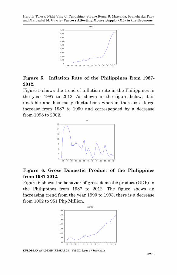
Figure 5. Inflation Rate of the Philippines from 1987-

2012.

Figure 5 shows the trend of inflation rate in the Philippines in

the year 1987 to 2012. As shown in the figure below, it is

unstable and has ma y fluctuations wherein there is a large

increase from 1987 to 1990 and corresponded by a decrease

from 1998 to 2002.

Figure 6. Gross Domestic Product of the Philippines

from 1987-2012.

Figure 6 shows the behavior of gross domestic product (GDP) in

the Philippines from 1987 to 2012. The figure shows an

increasing trend from the year 1990 to 1993, there is a decrease

from 1002 to 951 Php Million.

0

10,000

20,000

30,000

40,000

50,000

60,000

70,000

80,000

90,000

88 90 92 94 96 98 00 02 04 06 08 10 12

FER

900

1,000

1,100

1,200

1,300

1,400

1,500

1,600

88 90 92 94 96 98 00 02 04 06 08 10 12

GDPPC

2

4

6

8

10

12

14

16

88 90 92 94 96 98 00 02 04 06 08 10 12

IR




3279

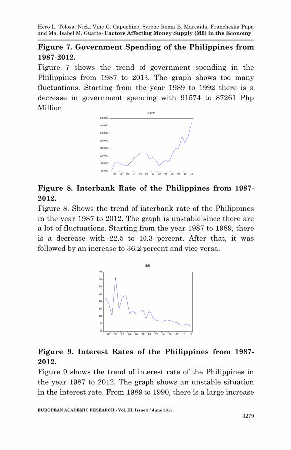
Figure 7. Government Spending of the Philippines from

1987-2012.

Figure 7 shows the trend of government spending in the

Philippines from 1987 to 2013. The graph shows too many

fluctuations. Starting from the year 1989 to 1992 there is a

decrease in government spending with 91574 to 87261 Php

Million.

Figure 8. Interbank Rate of the Philippines from 1987-

2012.

Figure 8. Shows the trend of interbank rate of the Philippines

in the year 1987 to 2012. The graph is unstable since there are

a lot of fluctuations. Starting from the year 1987 to 1989, there

is a decrease with 22.5 to 10.3 percent. After that, it was

followed by an increase to 36.2 percent and vice versa.

0

5

10

15

20

25

30

35

40

88 90 92 94 96 98 00 02 04 06 08 10 12

IBR

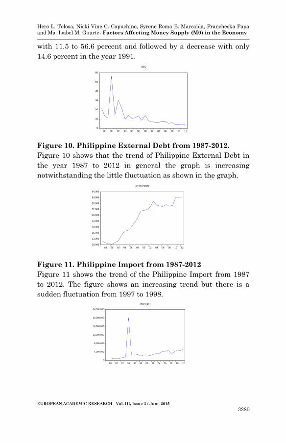
Figure 9. Interest Rates of the Philippines from 1987-

2012.

Figure 9 shows the trend of interest rate of the Philippines in

the year 1987 to 2012. The graph shows an unstable situation

in the interest rate. From 1989 to 1990, there is a large increase

80,000

90,000

100,000

110,000

120,000

130,000

140,000

150,000

88 90 92 94 96 98 00 02 04 06 08 10 12

GSPH




3280

with 11.5 to 56.6 percent and followed by a decrease with only

14.6 percent in the year 1991.

Figure 10. Philippine External Debt from 1987-2012.

Figure 10 shows that the trend of Philippine External Debt in

the year 1987 to 2012 in general the graph is increasing

notwithstanding the little fluctuation as shown in the graph.

Figure 11. Philippine Import from 1987-2012

Figure 11 shows the trend of the Philippine Import from 1987

to 2012. The figure shows an increasing trend but there is a

sudden fluctuation from 1997 to 1998.

0

10

20

30

40

50

60

88 90 92 94 96 98 00 02 04 06 08 10 12

IRS

28,000

32,000

36,000

40,000

44,000

48,000

52,000

56,000

60,000

64,000

88 90 92 94 96 98 00 02 04 06 08 10 12

PEDUSDM

0

4,000,000

8,000,000

12,000,000

16,000,000

20,000,000

24,000,000

88 90 92 94 96 98 00 02 04 06 08 10 12

PIUSSDT




3281

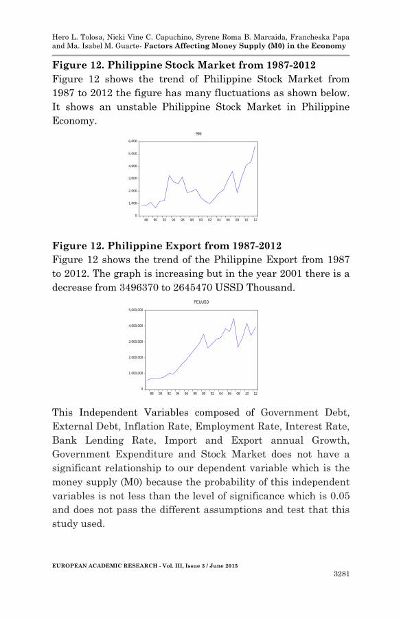
Figure 12. Philippine Stock Market from 1987-2012

Figure 12 shows the trend of Philippine Stock Market from

1987 to 2012 the figure has many fluctuations as shown below.

It shows an unstable Philippine Stock Market in Philippine

Economy.

Figure 12. Philippine Export from 1987-2012

Figure 12 shows the trend of the Philippine Export from 1987

to 2012. The graph is increasing but in the year 2001 there is a

decrease from 3496370 to 2645470 USSD Thousand.

This Independent Variables composed of Government Debt,

External Debt, Inflation Rate, Employment Rate, Interest Rate,

Bank Lending Rate, Import and Export annual Growth,

Government Expenditure and Stock Market does not have a

significant relationship to our dependent variable which is the

money supply (M0) because the probability of this independent

variables is not less than the level of significance which is 0.05

and does not pass the different assumptions and test that this

study used.

0

1,000,000

2,000,000

3,000,000

4,000,000

5,000,000

88 90 92 94 96 98 00 02 04 06 08 10 12

PEUUSD

0

1,000

2,000

3,000

4,000

5,000

6,000

88 90 92 94 96 98 00 02 04 06 08 10 12

SM




3282

Independent Variables that have a SIGNIFICANT

relationship with the Dependent Variable.

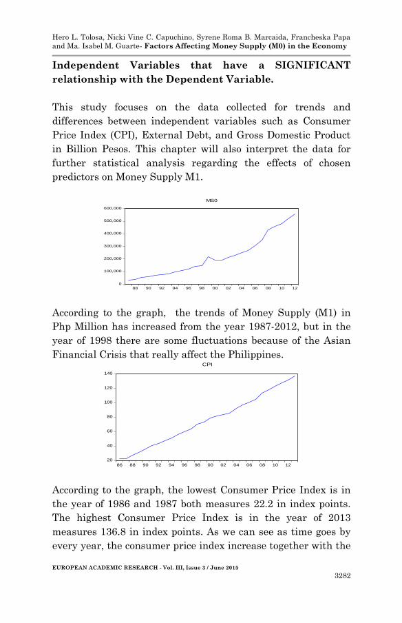
This study focuses on the data collected for trends and

differences between independent variables such as Consumer

Price Index (CPI), External Debt, and Gross Domestic Product

in Billion Pesos. This chapter will also interpret the data for

further statistical analysis regarding the effects of chosen

predictors on Money Supply M1.

0

100,000

200,000

300,000

400,000

500,000

600,000

88 90 92 94 96 98 00 02 04 06 08 10 12

MS0

According to the graph, the trends of Money Supply (M1) in

Php Million has increased from the year 1987-2012, but in the

year of 1998 there are some fluctuations because of the Asian

Financial Crisis that really affect the Philippines.

20

40

60

80

100

120

140

86 88 90 92 94 96 98 00 02 04 06 08 10 12

CPI

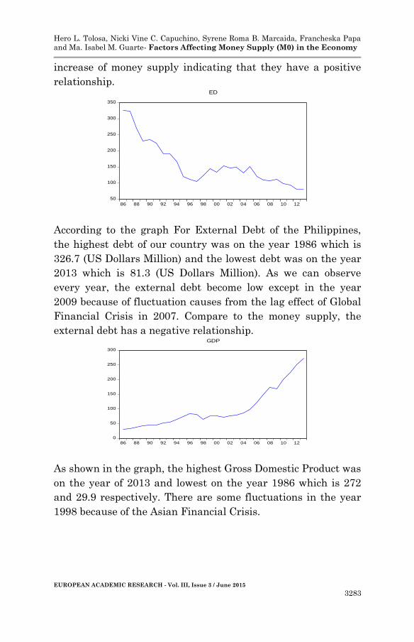
According to the graph, the lowest Consumer Price Index is in

the year of 1986 and 1987 both measures 22.2 in index points.

The highest Consumer Price Index is in the year of 2013

measures 136.8 in index points. As we can see as time goes by

every year, the consumer price index increase together with the




3283

increase of money supply indicating that they have a positive

relationship.

50

100

150

200

250

300

350

86 88 90 92 94 96 98 00 02 04 06 08 10 12

ED

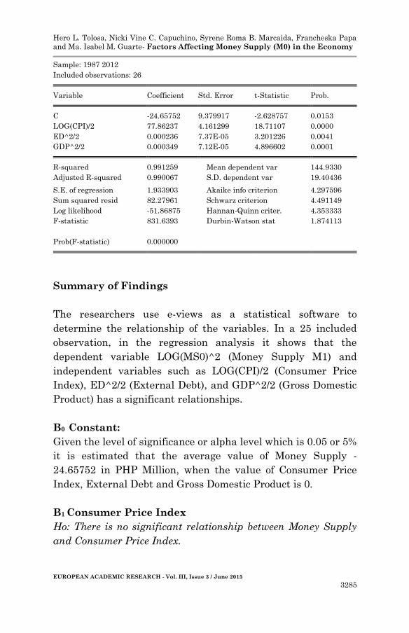
According to the graph For External Debt of the Philippines,

the highest debt of our country was on the year 1986 which is

326.7 (US Dollars Million) and the lowest debt was on the year

2013 which is 81.3 (US Dollars Million). As we can observe

every year, the external debt become low except in the year

2009 because of fluctuation causes from the lag effect of Global

Financial Crisis in 2007. Compare to the money supply, the

external debt has a negative relationship.

0

50

100

150

200

250

300

86 88 90 92 94 96 98 00 02 04 06 08 10 12

GDP

As shown in the graph, the highest Gross Domestic Product was

on the year of 2013 and lowest on the year 1986 which is 272

and 29.9 respectively. There are some fluctuations in the year

1998 because of the Asian Financial Crisis.




3284

MODEL SPECIFICATION

LOG(MS0)^2 = C(1) + C(2)*LOG(CPI)/2 + C(3)*ED^2/2 +

C(4)*GDP^2/2

Where:

MS0 = Money Supply (M0)

CPI= Consumer Price Index

ED= External Debt

GDP= Gross Domestic Product

MODEL ESTIMATION

LOG(MS0)^2 = -24.6575199324 + 77.8623735657*LOG(CPI)/2

+ 0.000236023636677*ED^2/2 + 0.000348514184232*GDP^2/2

For every change of 77.86237 in the LOG(CPI)/2 shows that

with the ED^2/2 and GDP^2/2 held constant/fixed, as the

LOG(CPI)/2 decrease in 1 point, Money Supply (m1)

LOG(MS0)^2 will increase 77.86237 in PHP Million Ceteris

Paribus

The coefficient 0.000236 of ED^2/2 shows that with the

LOG(CPI)/2 and GDP^2/2 constant/fixed, as the ED^2/2

increase 1 U.S Dollars (million), Money Supply (m1)

LOG(MS0)^2 will increase 0.000236 in PHP Million.

The coefficient 0.000349 of GDP^2/2 shows that with the

LOG(CPI)/2 and GDP^2/2 held constant/fixed, as the GDP^2/2

increase 1 PHP Billion, Money supply (m1) LOG(MS0)^2 will

increase 0.000349 in PHP Million.

Lastly, as all explanatory variables LOG(CPI)/2, ED^2/2

& GDP^2/2) where held fixed at zero, LOG(MSO)^2 would be -

24.65752 in PHP Million.

REGRESSION ANALYSIS

Dependent Variable: LOG(MS0)^2

Method: Least Squares

Date: 02/28/15 Time: 16:38




3285

Sample: 1987 2012

Included observations: 26

Variable Coefficient Std. Error t-Statistic Prob.

C -24.65752 9.379917 -2.628757 0.0153

LOG(CPI)/2 77.86237 4.161299 18.71107 0.0000

ED^2/2 0.000236 7.37E-05 3.201226 0.0041

GDP^2/2 0.000349 7.12E-05 4.896602 0.0001

R-squared 0.991259 Mean dependent var 144.9330

Adjusted R-squared 0.990067 S.D. dependent var 19.40436

S.E. of regression 1.933903 Akaike info criterion 4.297596

Sum squared resid 82.27961 Schwarz criterion 4.491149

Log likelihood -51.86875 Hannan-Quinn criter. 4.353333

F-statistic 831.6393 Durbin-Watson stat 1.874113

Prob(F-statistic) 0.000000

Summary of Findings

The researchers use e-views as a statistical software to

determine the relationship of the variables. In a 25 included

observation, in the regression analysis it shows that the

dependent variable LOG(MS0)^2 (Money Supply M1) and

independent variables such as LOG(CPI)/2 (Consumer Price

Index), ED^2/2 (External Debt), and GDP^2/2 (Gross Domestic

Product) has a significant relationships.

B0 Constant:

Given the level of significance or alpha level which is 0.05 or 5%

it is estimated that the average value of Money Supply -

24.65752 in PHP Million, when the value of Consumer Price

Index, External Debt and Gross Domestic Product is 0.

B1 Consumer Price Index

Ho: There is no significant relationship between Money Supply

and Consumer Price Index.




3286

Ha: There is a significant relationship between Money Supply

and Consumer Price Index

The Probability value of independent variable Consumer Price

Index (LOG(CPI)/2) is 0.0000 which is the perfect probability

that obviously less than the 0.05 or 5% alpha level or level of

significance. Therefore, we reject the null hypothesis, hence,

there is a significant relationship between Consumer Price

Index (LOG(CPI)/2) and Money Supply (LOG(MS0)^2).

For every 1 index point increase in the Consumer Price

Index (LOG(CPI)/2),coincide with the Money Supply

(LOG(MS0)^2). will also increase at 77.86237 in PHP Million

Ceteris Paribus.

B2 External Debt


and External Debt.


and External Debt.

The Probability value of independent variable External Debt

ED^2/2 is 0.0041 which is less than the 0.05 or 5% alpha level

or level of significance. Therefore, we reject the null hypothesis,

hence, there is a significant relationship between External Debt

(ED^2/2) and Money Supply (LOG(MS0)^2).

For every 1 US Dollars Million increase in the External

Debt (ED^2/2) coincide with the Money Supply

(LOG(MS0)^2).will also increase at 0.000236 in PHP Million

Ceteris Paribus.

B3 Gross Domestic Product


and Gross Domestic Product.


and Gross Domestic Product




3287

The Probability value of independent variable Gross Domestic

Product GDP^2/2 is 0.0001 which is less than the 0.05 or 5%

alpha level or level of significance. Therefore, we reject the null

hypothesis, hence, there is a significant relationship between

and Money Supply (LOG(MS0)^2).

For every 1 PHP Billion increase in the Gross Domestic

Product GDP^2/2 coincide with the Money Supply

(LOG(MS0)^2).will also increase at 0.000236 in PHP Million

Ceteris Paribus.

Ho: βi=0;All independent variables (Consumer Price

Index, External Debt and Gross Domestic Product) are not

predictors of dependent variable.(Money Supply M1).

Ha: βi≠0; All independent variables (Consumer Price

Index, External Debt and Gross Domestic Product) are

predictors of dependent variable (Money Supply M1).

Where i = 0, 1, 2…k and k-1 is the number of regressors.

The Probability value of F-statistics is 0.000000 which is

the perfect value of probability is greater than the 0.05 or 5%

alpha level or level of significance., Therefore ,we reject the null

hypothesis, and hence all independent variables (Consumer

Price Index, External Debt and Gross Domestic Product) are

predictors of dependent variable (Money Supply M1).

In interpreting goodness and fitness (R-squared), based

on the computed R-squared which is 0.991259 or 99.12 % of the

total variability of Money Supply is explained by the changes in

the Consumer Price Index, External Debt and Gross Domestic

Product.

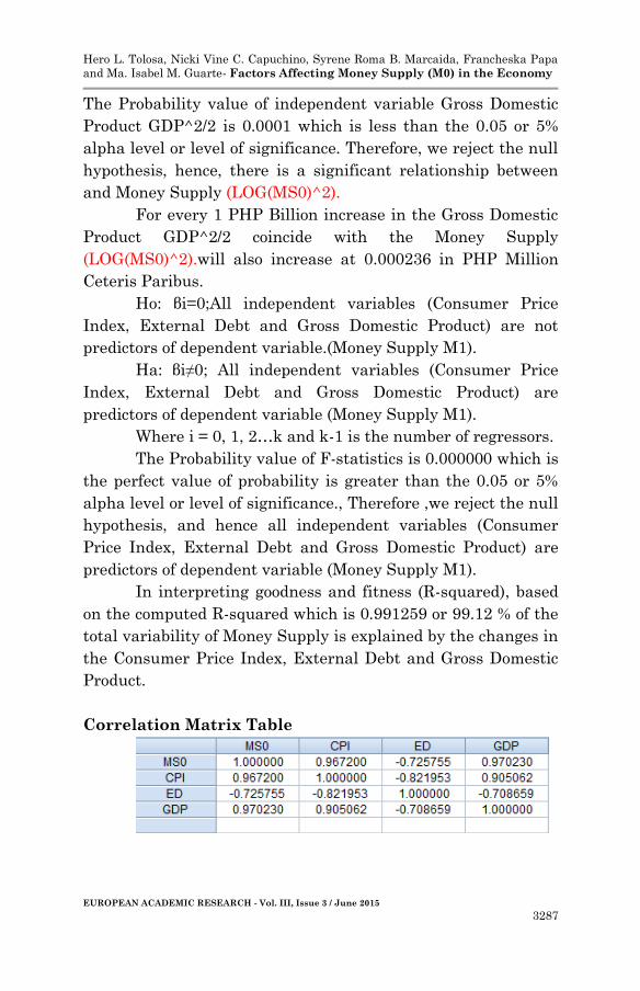
Correlation Matrix Table




3288

Hypothesis

Ho: =0 (There is no actual correlation)

Ha: 0 (There is a correlation)

According to the correlation matrix table, it shows that CPI has

0.967200 correlation coefficient and GDP has a 0.970230

correlation coefficient. Therefore, the CPI and GDP has a

strong/linear positive relationship with the MS0, thus the

variables move in the same direction when there is a positive

correlation.

Whereas, the ED has a -0.725755 correlation coefficient.

Therefore, the ED has a strong negative relationship with the

MS0, thus the variables move in opposite directions when there

is a negative correlation.

Therefore, because our independent variables are

correlated with our dependent variable, we reject the null

hypothesis.

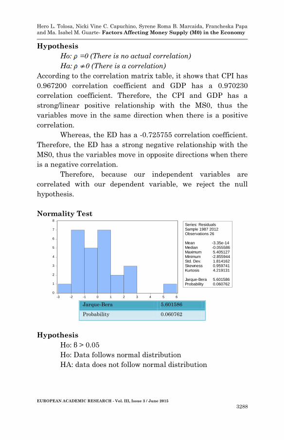
Normality Test

0

1

2

3

4

5

6

7

8

-3 -2 -1 0 1 2 3 4 5 6

Series: ResidualsSample 1987 2012Observations 26

Mean -3.35e-14Median -0.055586Maximum 5.405127Minimum -2.855944Std. Dev. 1.814162Skewness 0.959741Kurtosis 4.219131

Jarque-Bera 5.601586Probability 0.060762

Jarque-Bera 5.601586

Probability 0.060762

Hypothesis

Ho: β > 0.05

Ho: Data follows normal distribution

HA: data does not follow normal distribution




3289

The p-value is 0.060762 which is greater than the alpha or level

of significance of 0.05. The Jarque-Bera test, on the other hand,

shows that the JB Statistics is 5.601586 which is also greater

than the level of significance whch is 0.05 or 5%. Thus, we

failed to reject the null hypothesis (Ho) that the residual terms

are normally distributed. Data follows normal Distribution.

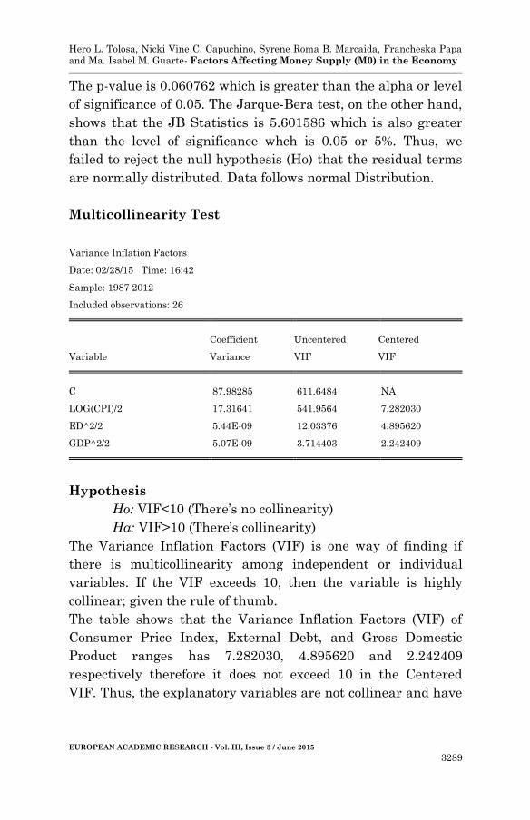
Multicollinearity Test

Variance Inflation Factors

Date: 02/28/15 Time: 16:42

Sample: 1987 2012


Coefficient Uncentered Centered

Variable Variance VIF VIF

C 87.98285 611.6484 NA

LOG(CPI)/2 17.31641 541.9564 7.282030

ED^2/2 5.44E-09 12.03376 4.895620

GDP^2/2 5.07E-09 3.714403 2.242409

Hypothesis

Ho: VIF<10 (There’s no collinearity)

Ha: VIF>10 (There’s collinearity)

The Variance Inflation Factors (VIF) is one way of finding if

there is multicollinearity among independent or individual

variables. If the VIF exceeds 10, then the variable is highly

collinear; given the rule of thumb.

The table shows that the Variance Inflation Factors (VIF) of

Consumer Price Index, External Debt, and Gross Domestic

Product ranges has 7.282030, 4.895620 and 2.242409

respectively therefore it does not exceed 10 in the Centered

VIF. Thus, the explanatory variables are not collinear and have




3290

significant relationship with each other. Hence, we fail to reject

the null hypothesis.

Durbin Watson Test

Durbin-Watson stat 1.874113

Hypothesis:

Ho: ρ = 0

Ha: ρ> 0

Durbin-Watson test is the most popular test in finding serial

correlation. For 25 observations and 3 individual variables,

with an alpha level of 0.05, Durbin-Watson Statistics of

1.874113 indicates that d is greater than the du and dl having

the values 1.408 and 0.906 respectively. Therefore, we fail to

reject the null hypothesis.

Ramsey RESET Test Ramsey RESET Test

Equation: UNTITLED

Specification: LOG(MS0)^2 C LOG(CPI)/2 ED^2/2 GDP^2/2

Omitted Variables: Squares of fitted values

Value df Probability

t-statistic 1.792457 21 0.0875

F-statistic 3.212902 (1, 21) 0.0875

Likelihood ratio 3.701443 1 0.0544

F-test summary:

Sum of Sq. df Mean Squares

Test SSR 10.91800 1 10.91800

Restricted SSR 82.27961 22 3.739982

Unrestricted SSR 71.36162 21 3.398172

Unrestricted SSR 71.36162 21 3.398172

LR test summary:

Value df

Restricted LogL -51.86875 22

Unrestricted LogL -50.01803 21




3291

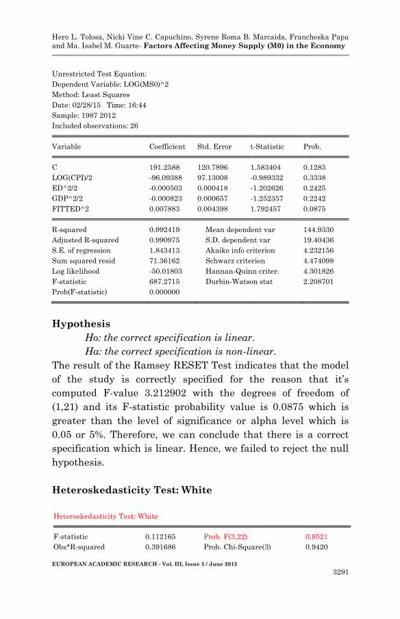
Unrestricted Test Equation:

Dependent Variable: LOG(MS0)^2


Date: 02/28/15 Time: 16:44

Sample: 1987 2012



C 191.2588 120.7896 1.583404 0.1283

LOG(CPI)/2 -96.09388 97.13008 -0.989332 0.3338

ED^2/2 -0.000503 0.000418 -1.202626 0.2425

GDP^2/2 -0.000823 0.000657 -1.252357 0.2242

FITTED^2 0.007883 0.004398 1.792457 0.0875


Adjusted R-squared 0.990975 S.D. dependent var 19.40436






Hypothesis

Ho: the correct specification is linear.

Ha: the correct specification is non-linear.

The result of the Ramsey RESET Test indicates that the model

of the study is correctly specified for the reason that it’s

computed F-value 3.212902 with the degrees of freedom of

(1,21) and its F-statistic probability value is 0.0875 which is

greater than the level of significance or alpha level which is

0.05 or 5%. Therefore, we can conclude that there is a correct

specification which is linear. Hence, we failed to reject the null

hypothesis.

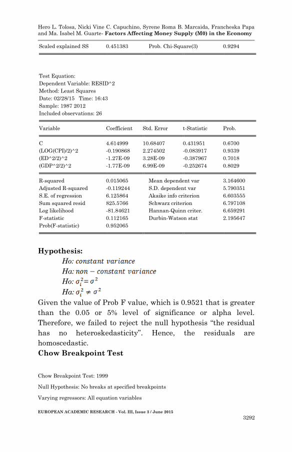
Heteroskedasticity Test: White

Heteroskedasticity Test: White

F-statistic 0.112165 Prob. F(3,22) 0.9521

Obs*R-squared 0.391686 Prob. Chi-Square(3) 0.9420




3292

Scaled explained SS 0.451383 Prob. Chi-Square(3) 0.9294

Test Equation:

Dependent Variable: RESID^2


Date: 02/28/15 Time: 16:43

Sample: 1987 2012



C 4.614999 10.68407 0.431951 0.6700

(LOG(CPI)/2)^2 -0.190868 2.274502 -0.083917 0.9339

(ED^2/2)^2 -1.27E-09 3.28E-09 -0.387967 0.7018

(GDP^2/2)^2 -1.77E-09 6.99E-09 -0.252674 0.8029


Adjusted R-squared -0.119244 S.D. dependent var 5.790351






Hypothesis:

Ho:

Ha:

Ho: =

Ha:

Given the value of Prob F value, which is 0.9521 that is greater

than the 0.05 or 5% level of significance or alpha level.

Therefore, we failed to reject the null hypothesis “the residual

has no heteroskedasticity”. Hence, the residuals are

homoscedastic.

Chow Breakpoint Test

Chow Breakpoint Test: 1999

Null Hypothesis: No breaks at specified breakpoints

Varying regressors: All equation variables




3293

Equation Sample: 1987 2012

F-statistic 2.786962 Prob. F(4,18) 0.0580

Log likelihood ratio 12.53224 Prob. Chi-Square(4) 0.0138

Wald Statistic 11.14785 Prob. Chi-Square(4) 0.0250

Hypothesis

Ho: No breaks at specified breakpoints

Ha: Have breaks at specified breakpoints

The Chow Breakpoint Test with the Probability of 0.0580 which

is greater than the 0.05 or 5% level of significance with the

degree of freedom of (4,18) indicating that the coefficients in

two linear regressions on different data sets are equal.

Therefore, we failed to reject the null hypothesis because there

is no break at the year 1999.

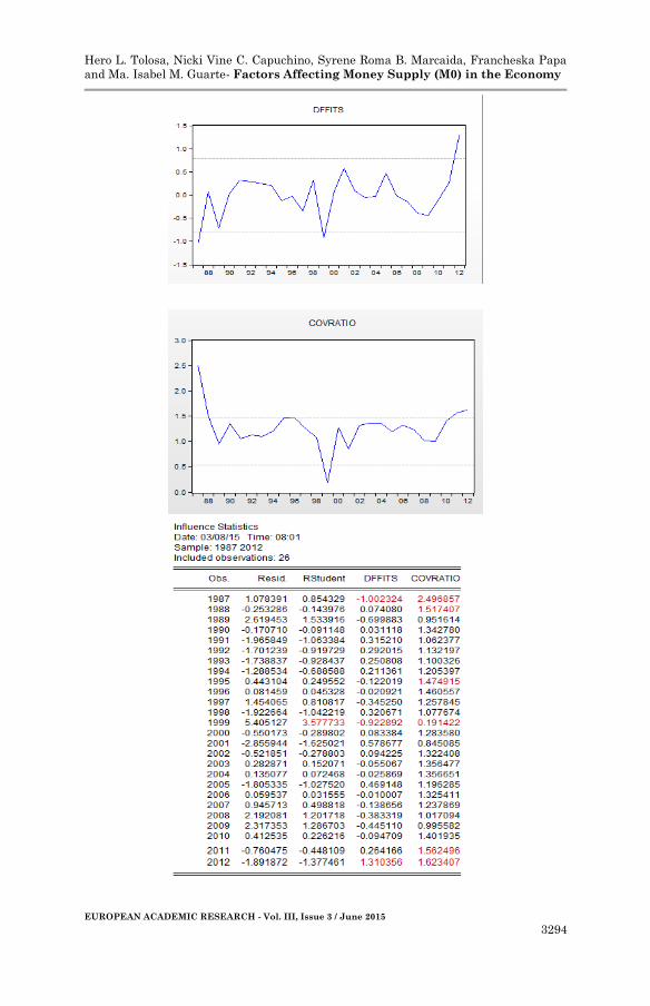
Outliers Test





3294




3295

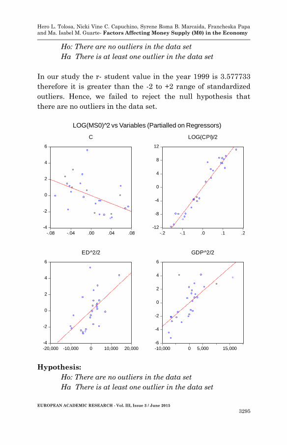
Ho: There are no outliers in the data set

Ha There is at least one outlier in the data set

In our study the r- student value in the year 1999 is 3.577733

therefore it is greater than the -2 to +2 range of standardized

outliers. Hence, we failed to reject the null hypothesis that

there are no outliers in the data set.

-4

-2

0

2

4

6

-.08 -.04 .00 .04 .08

C

-12

-8

-4

0

4

8

12

-.2 -.1 .0 .1 .2

LOG(CPI)/2

-4

-2

0

2

4

6

-20,000 -10,000 0 10,000 20,000

ED^2/2

-6

-4

-2

0

2

4

6

-10,000 0 5,000 15,000

GDP^2/2

LOG(MS0)^2 vs Variables (Partialled on Regressors)

Hypothesis:

Ho: There are no outliers in the data set

Ha There is at least one outlier in the data set




3296

Conclusion

The purpose of econometrics is to prove the economic

phenomena by presenting empirical evidence to support an

existing theory. In economics, a theory exists explaining that

macroeconomic variables are interdependent to each other on a

certain level of degree. In this paper, the researchers are trying

to test the level of various independent variables to a dependent

variable by presenting it in a numerical context.

Through statistical model the researchers have had

investigated the relationship between four key macroeconomic

variables (i.e. Money Supply, Consumer Price Index (CPI),

External Debt, and Gross Domestic Product) in the economy of

the Philippines.

In this study, the researchers conclude that the several

independent variables (Consumer Price Index (CPI), External

Debt, and Gross Domestic Product) have a high significance

level of relationship to the dependent variable (Money Supply)

having a prob (F-Statistics) of lower than 0.05 and an R-

Squared of 99.12 %. These variables could be predictors of the

money supply. Consequently, the certain changes in these

predictors could influence the behavior of money supply.

Recommendation

After a thorough study regarding the factors affecting the

money supply and based on the statistical results that the

researchers have conducted, this study is recommended

primarily to the Bangko Sentral ng Pilipinas, market

institutions and students.

Having the power to control over price, the researchers

suggests that market institutions must properly regulate prices

of the goods since these prices have a high influence/effect to

the economy's money supply(m0).




3297

This study is also recommended to the students that will have

their own study regarding or may be related with this study for

better understanding of some factors (the CPI, GDP and

External Debt) that may affect the money supply(m0).

This study is still open for rectification and

improvement. It could be recommended to the future

researchers in conducting a study correlated to this. This would

serve as their basis and/or their guide.

Bibliography

Aggarwal, Charu C. Outlier Analysis. New York, USA.

Coenders, Germa and Marc Saez. Collinearity,

Heteroscedasticity and Outlier Diagnostics In Regression:

Do they Always Offer What They Claim?2000.

Dufour, Jean-Marie. Generalized Chow Tests for Structural

Change: A Coordinate-Free Approach. 1982.

Escudero, Walter S. Conditional Expectations and Linear

Regression. 2009.Neilsen, Bent and Andrew Whitby. A

Joint Chow Test for Structural Instability. University of

Oxford, 2012.

Escudero, Walter S. Heteroskedasticity and Weighted Least

Squares. 2009.

Eyal, Katherine. Quantitative Methods for Economics. 2010.

Ismail, Haythem O. Reason Maintenance and the Ramsey Test.

Germany.

Kramarz, Francis and Michael Visser. The Linear Regression

Models. 2012.

Kriegel, Hans-Peter, Peer Kroger and Arthur Zimek. Outlier

Detection Techniques. Germany.

Neter, John, William Wasserman and Michael H. Kutner.

Applied Linear Regression Models. Illinois: Richard D.

Irwin, Inc., 1983.

Rubaszek, Michal. Applied Econometrics.




3298

Shapiro, S. S. and M. B. Wilk. An Analysis of Variance Test for

Normality. Biometrika, Vol. 52. 1965.

Stock, James H. and Mark W. Watson. Introduction to

Econometrics. Prentice Hall, 2008.

Tserkezos, Efstratios. Temporal Aggregation and the Ramsey’s

(RESET) Test for Functional Form:Result from Monte

Carlo experiment. University of Macedonia, Greece.

2009.

Documents

Factors Affecting Money Supply (M0) in the Economyeuacademic.org/UploadArticle/1737.pdfsituations that hinders economic growth. The researchers look into the best model in order to