FACTORS INFLUENCING THE PRICE OF LAND IN NAKURU

COUNTY

DENNIS MATHENGE WACHIRA

D61/79219/2015

A RESEARCH PROJECT SUBMITTED IN PARTIAL

FULFILLMENT OF THE REQUIREMENTS FOR THE AWARD OF

THE MASTER OF BUSINESS ADMINISTRATION DEGREE,

UNIVERSITY OF NAIROBI

NOVEMBER, 2017

ii

DECLARATION

This research project is my original work and it has not been presented for any academic

award in any university or institution of higher learning.

Signature: ........................................ Date: ............................................

Dennis Mathenge Wachira

D61/79219/2015

This research project has been presented for examination with my approval as the

University Supervisor.

Signature: .......................................... Date: ...........................................

Dr. Josephat Lishenga

Lecturer, Department of Finance and Accounting

School of Business

University of Nairobi

iii

ACKNOWLEDGEMENT

I wish to sincerely thank my supervisor Dr. Josephat Lishenga for his guidance and support

towards my research project: my close circle of friends who I learnt a great deal from and

my wife who challenges me to always achieve my full potential.

iv

DEDICATION

I dedicate this research project to all the people who value, advance and disseminate

knowledge all over the world.

v

TABLE OF CONTENTS

DECLARATION ................................................................................................................ ii

ACKNOWLEDGEMENT ................................................................................................. iii

DEDICATION ................................................................................................................... iv

LIST OF TABLES ............................................................................................................. ix

LIST OF FIGURES ............................................................................................................ x

LIST OF ABBREVIATIONS ............................................................................................ xi

ABSTRACT ...................................................................................................................... xii

CHAPTER ONE: INTRODUCTION ............................................................................. 1

1.1 Background of the study ............................................................................................... 1

1.1.1 Real Estate Prices ............................................................................................... 2

1.1.2 How the factors influence the price of real estate property ................................ 3

1.1.3 Real estate in Nakuru County ............................................................................. 4

1.2 Research Problem ......................................................................................................... 6

1.3 Research Objectives ...................................................................................................... 8

1.4 Value of the Study ........................................................................................................ 8

CHAPTER TWO: LITERATURE REVIEW .............................................................. 10

2.1 Introduction ................................................................................................................. 10

2.2 Theoretical Review ..................................................................................................... 10

2.2.1 The Agency Theory .......................................................................................... 10

2.2.2 Hedonic Model of Pricing ................................................................................ 11

2.2.3 Efficient Market Hypothesis ............................................................................. 12

2.3.4 Real Estate Property Appraisal or Valuation Theory ....................................... 14

vi

2.3 Determinants of Real Estate Property Prices .............................................................. 14

2.3.1 Speculative Investment Demand ...................................................................... 14

2.3.2 Proximity to Urban Center ............................................................................... 15

2.3.3 Interest Rates .................................................................................................... 15

2.3.4 Real GDP .......................................................................................................... 16

2.4 Empirical Review........................................................................................................ 16

2.5 Summary of Literature Review ................................................................................... 22

CHAPTER THREE: RESEARCH METHODOLOGY ............................................. 24

3.1 Introduction ................................................................................................................. 24

3.2 Research Design.......................................................................................................... 24

3.3 Population of the Study ............................................................................................... 24

3.4 Sample Design ............................................................................................................ 25

3.5 Data Collection Method .............................................................................................. 26

3.6 Validity and Reliability ............................................................................................... 26

3.7 Data Analysis .............................................................................................................. 26

3.7.1 Empirical Model .......................................................................................... 27

CHAPTER FOUR: DATA ANALYSIS, RESULTS AND DISCUSSION ................ 28

4.1 Introduction ................................................................................................................. 28

4.2 Response Rate ............................................................................................................. 28

4.3 Demographic Information ........................................................................................... 29

4.3.1 Gender .............................................................................................................. 29

4.3.2 Age.................................................................................................................... 29

4.3.3 Marital Status .................................................................................................... 30

vii

4.3.4 Level of Education ............................................................................................ 31

4.3.5 Employment Sector .......................................................................................... 32

4.3.6 The Ward Where Land is Situated ................................................................... 32

4.3.7 Size of land owned in the ward ........................................................................ 33

4.3.8 Period when the owner acquired the land ......................................................... 34

4.4 Descriptive Statistics ................................................................................................... 34

4.4.1 Speculative Investment Demand ...................................................................... 35

4.4.1.1 Price of Land ................................................................................................. 36

4.4.1.2 How the purchase was financed .................................................................... 36

4.4.1.3 What you intend to do with the land .............................................................. 37

4.4.1.4 Estimated value of the land ........................................................................... 38

4.4.2 Proximity to urban center ................................................................................. 38

4.4.2.1 Distance from the land to the road ................................................................. 39

4.4.2.2 What is the nature of the main road to your Land ......................................... 39

4.4.2.3 How near is the railway line to your land ...................................................... 40

4.4.2.4 Nearness of Naivasha town from your land .................................................. 40

4.4.3 Real GDP .......................................................................................................... 41

4.4.4 Lending Interest Rate ........................................................................................ 42

4.5 Correlation Analysis ................................................................................................... 43

4.6 Regression Analysis .................................................................................................... 44

4.6.1 Cross tabulation of Land price against estimated current price ........................ 44

4.6.2 Model Summary ............................................................................................... 45

4.6.3 Summary of ANOVA Results .......................................................................... 46

viii

4.6.4 Model Coefficients ........................................................................................... 47

4.7 Discussion of Findings ................................................................................................ 48

CHAPTER FIVE: SUMMARY OF FINDINGS, CONCLUSIONS AND

RECOMMENDATIONS ................................................................................................ 49

5.1 Introduction ................................................................................................................. 49

5.2 Summary of Findings .................................................................................................. 49

5.3 Conclusion of the Study and Policy Recommendation............................................... 50

5.4 Limitations of the study .............................................................................................. 50

5.5 Suggestions for Further Research ............................................................................... 51

REFERENCES ................................................................................................................ 51

APPENDICES ................................................................................................................. 55

APPENDIX I: QUESTIONNAIRE ............................................................................... 55

APPENDIX II: GDP IN MILLIONS ............................................................................ 57

ix

LIST OF TABLES

Table 4.1: Response Rate .................................................................................................. 28

Table 4.2: Real GDP (KSh Million) ................................................................................ 41

Table 4.3: Lending Interest Rate from CBK in % ............................................................ 42

Table 4.4: Correlation Matrix ........................................................................................... 43

Table 4.5: Cross tabulation of Price of land at the time of acquisition versus estimated

value of the land .............................................................................................. 44

Table 4.6: Model Summary .............................................................................................. 45

Table 4.7: Summary of ANOVA Results ......................................................................... 46

x

LIST OF FIGURES

Figure 4.1: Gender ............................................................................................................ 29

Figure 4.2: Age ................................................................................................................. 30

Figure 4.3: Marital Status ................................................................................................. 31

Figure 4.4: Level of Education ......................................................................................... 31

Figure 4.5: Employment Sector ........................................................................................ 32

Figure 4.6: Ward Name..................................................................................................... 33

Figure 4.7: Size of land owned in the ward ...................................................................... 33

Figure 4.8: The duration the land was acquired ................................................................ 34

Figure 4.9: Mode of Acquiring the Land .......................................................................... 35

Figure 4.10: Price of land.................................................................................................. 36

Figure 4.11: How the purchase was financed ................................................................... 37

Figure 4.12: What you intend to do with the land ............................................................ 37

Figure 4.13: Estimated value of the land .......................................................................... 38

Figure 4.14: Distance from the tarmac to your land ......................................................... 39

Figure 4.15: The nature of the main road to your land ..................................................... 39

Figure 4.16: Nearness of the railway line to your land ..................................................... 40

Figure 4.17: Nearness of Naivasha town from your land ................................................. 41

xi

LIST OF ABBREVIATIONS

CBK - Central Bank of Kenya

CPI - Consumer price index

GDP - Gross Domestic Product

HP - House Price

KNBS - Kenya National Bureau of Statistics

NCF - Net Cash Flow

NOI - Net Operating Income

OECD - Organization for Economic Cooperation and Development

UK - United Kingdom

USD - United States Dollars

xii

ABSTRACT

The objective of the study was to find out the factors influencing land prices in Nakuru

County. This was prompted by the recent upsurge of land prices in the country and the

researcher was particularly interested in Nakuru County. The real estate sector experiences

a series of booms and busts and it was therefore important to find out what is causing them.

The study aimed to cover several research gaps among them; whether the variables that

influence land value in mature markets like Japan are the same in Kenya, and apart from

the variables covered by local studies whether other variables like speculative investment

demand do influence land prices. The study adopted a descriptive study design and the

target population was the land owners in the four wards of Naivasha as shown in the county

government of Nakuru records. Sample was obtained using the stratified sampling method

to come up with the most representative sample. The dependent variable was the land price

while the independent variables were the speculative investment demand, interest rate,

proximity to urban center and real GDP. Data was collected from both primary and

secondary sources and analyzed using SPSS version 21.0 the model explained only 76.6%

of the relationship between the independent variables and the dependent variable. ANOVA

analysis showed that the probability of the value of 0.000 which was less than 0.05 which

indicated that the regression relationship was highly significant in predicting how

speculative investment demand, Interest rates, Proximity to urban center and Real GDP

influenced the price of land in Nakuru County. The findings of the study showed that all

the four independent variables had a significant positive relationship with land prices. The

study was therefore similar to studies done both internationally and locally. The researcher

therefore recommends that policy makers in government work on increasing the growth of

GDP. Commercial banks should lower the lending interest rate so that people can access

cheap loans and thus afford to buy land. Lastly, the government should endeavor to tarmac

all feeder roads to increase the value of land.

1

CHAPTER ONE

INTRODUCTION

1.1 Background of the Study

Pagourtzi, Assimakopoulos, Hatzichristos and French (2003) define real property as all

rights, benefits, interests, and hindrances intrinsic in the possession of physical real estate,

in which case real estate is the land jointly with all developments that are permanently

attached to it and all accessories contained in it. Investors also acquire some rights when

they invest in real estate, these rights are: developing, leasing, improving, controlling,

exploiting, occupying, selling, and pledging. All these rights have evolved to become

property rights (Brueggeman & Fisher, 2011).

The market for real estate is not the same as other financial markets in several ways. It is

extremely heterogeneous because of its physical attributes and location. Traders in that

market are met with illiquidity, huge transaction costs, carrying costs, taxes, and search

costs that arise from real estate’s heterogeneity. All these costs are frictions that point out

towards a market that is not efficient compared to other financial markets (Ghysels, Plazzi,

Torus & Valkanov 2012).

Real estate is an important international and local asset estimated to be about 55 percent of

world assets (Bao, Glascock, Zhou and Feng, 2015). The prices of real estate have more

than doubled in the past few years in Kenya and this stirs some pertinent questions on what

is causing the upswing in prices. Realtors and brokers play a large part in influencing the

price since they act on behalf of the buyers and sellers. The expansion in the sector for real

2

estate is being fueled by: a strong economy, protection of property law, an emerging middle

class, a robust banking sector, urbanization, and mega infrastructure projects by the

government (Omboi & Kigige, 2011).

This study will be based on several theories which include the agency theory, the hedonic

model of pricing theory, efficient market hypothesis and lastly real estate property appraisal

or valuation theory. Several studies have been done on real estate property in Kenya

touching on various topics but none has been done on the factors influencing land prices in

Nakuru County. This study therefore seeks to establish those factors and also find out if

the market for real estate in Nakuru behaves like other parts of Kenya that have been

targeted in previous studies or is different.

1.1.1 Real Estate Prices

Malpezzi and Watcher (2005) define price as the assets value which is equal to what the

economic players are willing to pay for real estate property. According to (Jennergren,

2011) the income approach is highly preferred by investors as a valuation technique and is

closely similar to the discounted cash flow analysis carried out on bond and equity

investments by both appraisers of commercial properties and underwriters of real estate

backed investments. The process of valuation starts by forecasting the income from the

property which can be the projected lease payments or for hotels the anticipated occupancy

multiplied by the mean cost of the room. Then, subtracting all the property level costs plus

the cost of finance leaves the net operating income (NOI) or cash flow net of operating

expenses. When all capital costs plus any investment capital used in the maintenance or

3

repair of the property and all other indirect expenses from NOI are subtracted the result is

the net cash flow (NCF). Since cash is not retained for properties or a dividend policy

applied NCF is equal to the cash available to investors and is similar to cash from dividends

which is used in valuing equity or fixed income investments. The property value is

determined when dividends are capitalized or cash flow streams (inclusive of any residual

value) are discounted during a certain investment period. (Dean, 2014).

1.1.2 How the factors influence the price of real estate property

The hedonic model of pricing theory comes out clearly between real estate pricing and the

factors that influence the prices. (Lancaster, 1966) argues that utility is not automatically

created by a good but by the individual characteristics of that good. To be specific a good

or item’s utility is basically the sum of the individual utility of each of its characteristics.

This theory has been shown to hold by (Choy, Mak and Ho, 2007) who carried out a

research in Hong Kong using the hedonic price model and all the variables were found to

be statistically significant. In addition , (Li, 2008) in his study finds out there are other

ways to the estimation of the price of land other than location convenience in an urban

modern economic perspective. Owing to progress in technology, and particularly in

telecommunication sector and a land market that is growing in the intricacy of its

composition, the market has produced new factors affecting land price behavior. Therefore,

it’s important to observe the land price behavior from new angle.

4

The agency theory has also been shown to hold between the real estate prices and the

factors influencing the prices. This relationship arises due to there being no centralized

market for exchange of real estate therefore buyers and sellers have to pay significant

search costs in the form of brokerage commissions and time. The informational friction is

also made worse by the heterogeneity and asymmetry of the quality of real estate, which

increases the cost of quality search and contracting substantially (Chau, Wong &Yiu,

2003).

The size of the parcel is traditionally recognized as an important determinant of land value:

the second determinant is location and it generally acts as a proxy of the economic and

social characteristics of the neighborhood of the land parcel. Thirdly, government

regulations also participate in determining the value of land (Bao, et al. 2015). It is therefore

evident that land prices are influenced by many factors which differ in relevance. This

empirical evidence shows that there exists a connection between the theory of real estate

appraisal or valuation and the factors influencing real estate prices.

1.1.3 Real estate in Nakuru County

The real estate sector undergoes a cycle of booms and busts. For instance Eveready East

Africa, a battery manufacturing company located in Nakuru town, closed shop owing to

stiff competition from cheap imports. The company has shelved its plan to build a shopping

mall on is prime land that was to be a mix use development comprising of apartments and

a shopping mall. Instead it would convince shareholders to sale the land and offset a costly

debt and provide free cash flows for investing in other sectors (Muhoro, 2016).

5

Upcoming gated community estates that are meant for middle and upper classes include

the Italian luxury court five kilometers from Naivasha town. The demand for houses has

also pushed up land prices especially by developers of holiday homes who have increased

their activities in Navasha (Gitonga, 2014). It is therefore important to find out what these

factors are and how they are influencing real estate property prices as it is a very important

asset class (Bao et al, 2015).

Studies done that look at the variables that might influence property prices include (Ho &

Ganesan1998) who carried out a study on the supply of land and residential housing prices;

they found out that speculative demand for housing has a significant but modest impact on

housing prices. This conclusion was also arrived at by (Levin & Wright 1997) who

formalized the method which shows how price speculation occurs in the market for housing

and provided some evidence on how the speculation is a possible determinant of housing

prices in London and the rest of the UK housing markets.

In another study, (Li, 2009) find out that closeness to CBD increases the value of real estate

as the transport cost is lower. The distance from the urban center where the land is located

is a major independent factor where readiness to purchase a specific piece of land at a

certain price level depends. Consequently, a tenant is able to bid a higher rent when

economic activities depend a lot on meeting the customers as first and as frequently as

possible owing to the closeness to the city center. Li (2015), in his study finds out that

interest rates have a major influence on real estate developers who provide housing in the

real estate market. He further argues that when interest rates increase, the real estate

6

developers construction costs increases thus driving up the price of real estate property. On

the other hand, buyers are faced with higher cost of purchasing houses and more pressure

in repaying their loans which balloons with additional interest rates. Therefore, the

increase in interest rates lowers the demand for house purchase and the decline of house

prices.

The overall economic activity is measured through GDP. Therefore, when there is change

in real GDP, it translates into a change in real economic expansion which usually affects

the real estate property market. Furthermore, there is increased business confidence

brought by economic certainty as a result of an increase in real GDP. From the foregoing

it is argued that demand for real estate property can be pushed up by an expansion in the

economy, which leads to house prices going up and consequently the returns, ceteris

paribus. In addition, the growth in real GDP means that the tenants’ ability to pay increases

which also causes the general rates in rent to go up, ceteris paribus. Thus, one can expect

a positive relationship between changes in real GDP and returns from housing property

(Clerk and Daniel, 2006).

1.2 Research Problem

This study aims at identifying the factors that influence real estate property prices. These

factors are anchored in theory as shown in 1.1.2 From the foregoing this study will look at

the following variables: speculative investment demand, proximity to urban center, interest

rates and real GDP and try to establish whether there is a significant relationship between

these factors and the real estate property prices in Nakuru county. Real estate has always

7

attracted a lot of interest in the global context and among the studies conducted

internationally that try to identify the factors influencing real estate property prices include

(Li and Chiang, 2012) who studied the factors behind China’s real estate price appreciation

in the duration 1998 to 2009 on a monthly basis. Their findings indicate that the real estate

prices in China are pushed up by both institutional and economic factors. They recommend

that a research be done to focus on two directions : first the impacts of land or disposable

income on real estate price; second the objectives of monetary and fiscal policies on

housing price by using a recently adopted econometric approach of factor- augmented

vector autoregressive (FAVAR) model for analysis.

This study will try to address these gaps by looking at land prices and what influences it.

Hidano and Yamamura (2004) did an analysis using a hedonic pricing model on changes

in land prices in Japan which is a mature market and discovered besides other variables,

lending behavior by banks and industrial investment activities was the cause for explaining

the major effect on the changes in land value. In order to carry out a robust analysis they

noted that it was important to access enough and reliable transaction data. Therefore, this

research will try to fill the gap by gathering enough transaction data to conduct the study.

In the Kenyan context, studies done on the real estate sector include Julius (2012) who

studied the determinants of residential real estate prices in Nairobi and pointed out that

further research should be done to cover Kenya and also the study should extend the time

horizon. Money supply as one of the factors in her model had no relationship with what

determines real estate prices. Muthee (2012) who sought to explain the relationship

8

between economic growth and prices of real estate in Kenya suggests further research

should be carried out for a longer duration and on a year to year basis.

A further research should be done on real estate sector policy on national economy. Marete

(2011) on a study of what determines the prices of real estate property in Kiambu

Municipality in Kenya suggests that comparative research be done between real estate

property prices in the rural areas and those in the urban areas and find out if the prices are

affected by the same factors. This research study aims at filling these gaps by answering

the following research question: what are the factors influencing real estate property prices

in Nakuru county?

1.3 Research Objectives

The objective of the study was to find out the factors influencing the price of land in

Nakuru County. The specific objectives were to find out if Speculative investment

demand, interest rates, real GDP and proximity to urban center influence land prices.

1.4 Value of the Study

This study will be valuable to investors in the real estate sector who will benefit immensely

as they will discover what drives property prices. This information will improve their

investment decisions and strategies.

9

Property owners will also benefit as they will be better informed on what affects the price

of their properties. This information will help property owners to price their properties

efficiently and thus get the optimum price.

The financial sector will also benefit, banks may find this study relevant because real estate

comprises a very big chunk of their collateral, investment funds will also benefit since real

estate is one of the component of their investment portfolios. Government policy makers

will be better placed to make strategic decisions when they are formulating policies on real

estate. Tax agents will know how to plan their tax policies based on the factors that affect

real estate prices when coming up with taxes on real estate.

This study will also be valuable to other students who wish to refer to the literature review

and also as a basis for further research owing to the limitations or to expand on the study.

10

CHAPTER TWO

LITERATURE REVIEW

2.1 Introduction

In this section both the theoretical and empirical review of literature was covered in the

area of real estate property sector. The aim of the review was to understand the theory

behind real estate and also confirm whether the theories have been proved empirically.

2.2 Theoretical Review

The research study was anchored on four theories that formed the basis for theoretical

foundation. The theories included: agency theory, hedonic model of pricing, efficient

market hypothesis and real estate property appraisal or valuation theory.

2.2.1 The Agency Theory

In their seminal paper Jensen and Meckling in 1976 proposed that the relationship

between principals and agents in business is explained by the supposition of the agency

theory. When an agent acts for, on behalf of, or as a representative for the other, identified

as a principal, in a particular area of solving problems through decision making then there

exists an agency relationship between them. The theory looks at how to ensure that agents

(realtors and brokers) act in the best interests of the principals (home and land owners) in

the real estate market. This theory is very relevant since the real estate sector is a classic

example of conflict of interest between the principal who is the seller of a house or land

and the agent who is the real estate broker.

11

In a research carried out by (Arnold, 1992) while looking at the agent - principal

relationship between a home owner and a broker, the study revealed two principal-agent

problems between them. The first problem was that the broker who is the agent may have

an incentive to offer minimal effort in providing current market information about the

search activity if the owner of the house is not keen on the brokers search activity. The

second problem arose from the fact that owners of homes participate in the market

infrequently and therefore they lack full information on demand and supply conditions in

the housing market while brokers are seasoned participants who are better informed about

the market conditions. House owners therefore rely on brokers to set up a reservation price.

This information asymmetry can lead to brokers being enticed to misinterpret the market

information to the detriment of the house owner. The agency theory is therefore relevant

as it shows how property prices are set between agents and principles.

2.2.2 Hedonic Model of Pricing

Lancaster’s seminal paper in 1966 was the beginning of an attempt to build a theoretical

foundation for hedonic modeling. He presented a ground breaking theory of hedonic utility.

In his argument he states that it is not always the case that a good creates utility by its self

but instead it is the individual characteristics of a good that creates the utility. A good or

item’s utility to be specific is basically the sum of the individual utility of each of its

characteristics. He further went on to argue that things such as goods or services can be

categorized depending on the characteristics they hold. He noted that consumers while

making a purchase decision refer to the group they belong to depending on the

characteristics a good possesses per unit cost.

12

Even though Lancaster was the first to discuss hedonic utility, he didn’t extend it to a

pricing model. Rosen (1974) using the hedonic model of house prices approximates the

implied price of every property characteristic by regressing transaction prices of properties

on equivalent property characteristic. Hedonic models are best suited for markets in which

a commodity can be embedded with varying amounts of each of a vector of utility-bearing

attributes. This model has been widely accepted in the research for housing to investigate

social ills like, ease of access to employment, neighborhood change, and racial

discrimination. A property for residential use can be viewed as a package of utility

producing attributes that are desired by consumers. The attributes are normally

characterized by durability, spatial fixity, physical rigidity and when they are mixed

differently they produce a good that is heterogeneous. The physical attributes of houses

alone cannot fully explain the variations of prices since prices of houses are influenced by

many intrinsic and outside factors. For instance, a change in relative price as a result of a

lower transport cost due to the linkage of the suburban areas to urban areas by the

introduction of a subway or highway is probably going to lead to homebuyers adjusting

their combination of housing attributes to the new optimum and as well as switch their

choice of residence. (Choy, et al., 2007).

2.2.3 Efficient Market Hypothesis

Fama (1970) in his seminal paper on efficient market hypothesis (EMH) is credited as

contributing a lot to modern finance. EMH is the idea that securities prices reflect all

available information. He argues that in EMH competition between investors looking for

supernormal profits leads to prices going to their “correct” value, therefore eliminating any

13

arbitrage opportunities as soon as they arise. Hence, a market is considered efficient in

relation to some information if the same information cannot enable investors earn abnormal

returns in comparison to the other investors. On the other hand when investors have insider

information they can use it to participate in insider trading thus having the ability to earn

excess positive returns.

Statman (1999) argues that market efficiency is the bone of contention among traditional

finance, investment professionals and behavioral finance. In contention is the concept of

“market efficiency” which he says has two meanings and one of them is that an investor

cannot outperform the market systematically, while the other meaning is that the prices for

securities are rational meaning that they display only “fundamental” or “utilitarian”

characteristics, for example risk, but not “value expressive” or “psychological”

characteristics like sentiment. Statman dismisses this second meaning.

This theory is useful in explaining investors’ sentiment especially when it comes to pricing

real estate property prices as shown by (Baker & Wurgler, 2006) who define investor

sentiment as the inclination to speculate or as trading on a belief relating to future cash

flows or risks that are not warranted by the existing facts.(Brown and Cliff, 2004) define

investor sentiment as the speculators bias, described as excessive optimism or

pessimism.Sentiment is investor expectations driven by irrational factors. Conventional

financial markets presume that asset prices mirror existing public information and that

rational investors prize assets fairly (Fama, 1979). On the contrary investors’ belief about

14

expectations of market movement are based on sentiments, which is different from the

investors’ risk aversion that measures their taste for risky assets over risk-free assets.

2.3.4 Real Estate Property Appraisal or Valuation Theory

Baum, (1995) his seminal paper defines real estate appraisal or valuation as the procedure

of valuing real estate property. The property's market value is what is usually vital. Property

appraisals are required because unlike company stock, transactions in real estate do not

occur frequently. In addition, there is a difference between one property to the next, an

aspect that is absent in assets like corporate stock. Also, all properties are fixed in different

locations which are an important part that determines their value. Due to the

aforementioned nature of real estate property, appraisers who are qualified specialists are

needed to advice on the value of a property. The appraiser usually presents a report on the

value of the property to their client. The reports are the basis for issuing mortgage loans,

for tax matters, for settling estates and divorces. The report from an appraiser sometimes

is referred to by both parties to arrive at the sale price of the property.

2.3 Determinants of Real Estate Property Prices

2.3.1 Speculative Investment Demand

Ho and Ganesan, (1998) carried out a study on the supply of land and residential housing

prices; they found out that speculative demand for housing has a significant but modest

impact on housing prices. This conclusion was also arrived at by (Levin &s Wright 1997)

who formalized the method which shows how price speculation occurs in the market for

15

housing and provided some evidence on how the speculation is a possible determinant of

housing prices in London and the rest of the UK housing markets.

2.3.2 Proximity to Urban Center

Closeness to CBD increases the value of real estate as the transport cost is lower. The

distance from the urban center where the land is located is a major independent factor

where readiness to purchase a specific piece of land at a certain price level depends.

Consequently, a tenant is able to bid a higher rent when economic activities depend a lot

on meeting the customers as first and as frequently as possible owing to the closeness of

the city center (Li, 2009).

2.3.3 Interest Rates

Li, 2015 in his study finds out that interest rates have a major influence on real estate

developers who provide housing in the real estate market. He further argues that when

interest rates increase, the real estate developers construction costs increases thus driving

up the price of real estate property. On the other hand, buyers are faced with higher cost of

purchasing houses and more pressure in repaying their loans which balloons with

additional interest rates. Therefore, the increase in interest rates lowers the demand for

house purchase and the decline of house prices. (Ding, 2014) finds that the loans borrowed

by real estate investors are huge and they account for about 40% to 60% of the total

proportion of loans in that particular year.

16

Further, there is a direct influence on the amount invested on real estate and the supply of

real estate property as a result of the lending rate. Also a slight adjustment on the rate of

interest has a significant impact on the real estate market. There will be a tendency for the

government to use interest rates through fiscal policies to regulate the real estate sector. In

this research interest rate is a major variable that influences the real estate property prices

and therefore its effect will be investigated to check whether there is a significant effect on

property prices.

2.3.4 Real GDP

The overall economic activity is measured through GDP. Therefore, when there is change

in real GDP, it translates into a change in real economic expansion which usually affects

the real estate property market. Furthermore, there is increased business confidence

brought by economic certainty as a result of an increase in real GDP. From the foregoing

it is argued that demand for real estate property can be pushed up by an expansion in the

economy, which leads to house prices going up and consequently the returns, ceteris

paribus. In addition, the growth in real GDP means that the tenants’ ability to pay increases

which also causes the general rates in rent to go up, ceteris paribus. Thus, one can expect

a positive relationship between changes in real GDP and returns from housing property

(Clerk and Daniel, 2006).

2.4 Empirical Review

Choy, Mak and Ho (2007) did a research from a Hong Kong perspective to approximate

the prices of real estate. A model based on hedonic pricing to estimate the implicit price of

17

each property characteristic was employed. The data was from Quarry Bay District which

was used as a case study. Other than the single mega-scale housing estate the district also

comprises of many small and medium scale estates. The data series was calculated for the

duration starting from July 1999 to June 2000, producing749 cross-sectional observations

in total. Data was analyzed using Newey–West Heteroskedasticity Consistent Covariance

and most variables were found to be statistically significant. These variables were: age,

sea, garden, mass transport railway and fengshui. The Fengshui variable which is a deeply

rooted traditional Chinese culture involving numbers and luck is not relevant to the Kenyan

real estate context.

Li, (2009), in his study scrutinizes land prices changes in Beijing from 1993 – 2004. He

uses regression analysis. The dataset is derived from the urban part of Beijing the period

covered is from 1993 all the way to the first half of 2005. 5,269 in total of transactions

including most of the commercial, mix use and residential land use types were used. To

begin with, using box–cox transformation in regression to convert data into approximately

normal distribution so that the data is more useful in statistical techniques based on the

normality assumption, the box–cox model compared with the simple linear regression is a

better fit of the original data. Secondly using a simple linear regression the results show

that population has negative significance in all types of use other than on commercial land

price where the variable in question is not shown to be statistically significant. In all

categories of land use types GDP was statistically significant. Local financial revenue and

wage levels are observed to be only significant in the price of industrial land.

18

There is a negative correlation between total investment in fixed assets and land prices in

residential and mix use land types. In conclusion, the findings indicate that prices in

residential land have been on a rising trajectory from 2000, signifying a robust demand for

housing as a result of a thriving economy in China. In contrast, insufficiency in

transactional data causes fluctuation in industrial land prices, on top of the fact that

transactions in industrial land are normally linked with projects by investors from other

countries where occasionally as an incentive, industrial land prices are set as a package that

does not indicate prevailing market value. Furthermore, prices in commercial land exhibit

a certain degree of fluctuation indicating that the nature of the real estate economy is

normally volatile. In Beijing, statistical analysis points towards land prices being affected

by market indicators such as investment and GDP growth. The researcher encounters a

problem with lack of adequate market data on land transactions. This study is applicable to

the Kenyan context as it shows a lot of similarity with the Kenyan real estate sector and

the insufficiency of data on land prices is not applicable to since data is available.

Pavlov and Watcher (2010) while looking at the US real estate sector uses the version of

the Longstaff and Schwartz (2001) least-squares simulation approach then applies

regression analysis found out that the bank’s lending sector developed new capability to

present through financial innovation and deregulation aggressive products. Specifically,

automated underwriting models made it possible to implement risk-based pricing, leading

to the lending of mortgages that were riskier becoming prevalent in the late 1990s

following the development of private label securitization of nonconforming loans. In the

similar period, banks were allowed through deregulation to originate and securitize these

19

mortgages exclusive of having to account for the buyback requirements entrenched in these

securities. In their conclusion, the availability of more funds to the borrower from banks

increases the demand for more homes that ends up causing an upsurge in prices especially

in a market with a fixed or inelastic supply. This study is very relevant because the

automation and financial innovation is similar to what is going on with the Kenyan banking

sector.

Li and Chiang, (2012) looks at the factors encouraging China’s real estate price

appreciation from 1998 to 2009 from month to month. They use Granger causality test, co-

integration approach, vector error correction model, to investigate whether stable and long-

run equilibrium relations are present between prices in housing and fundamental macro-

economic variables, for instance GDP, CPI and land sale. A bilateral Granger causality is

evident between HP and CPI. However, GDP does not Granger cause HP, showing

personal gain (disposable income) does not draw level with national gain (GDP) in China.

Co integration analysis indicates long-term equilibrium between the price of real estate

(HP) and CPI or GDP, but not land sale. Between HP to GDP there is no feedback effect,

indicating housing price appreciation does not translate in immediate capital gain or

speculations in housing purchase. Moreover, lack of co integration relationships between

land sale and HP is possibly caused by restrictive policies on land supply. The real estate

price in China is pushed up by both institutional and economic factors. The institutional

factors that push up real estate prices in china are not present in Kenya since the market for

real estate in Kenya is free market.

20

Liu, Wang and Zha, (2013) look at land price changes and macroeconomic variations. They

are keen on land price since it causes the most change in a house price when it fluctuates

compared to the cost of the structure. In one of their observations, they note that there is

empirical evidence that shows that the changes in land price and macro-economic variables

move together not only during the US great recession, but also throughout the sample

period that covers the years from 1975 to 2010. Through a four variable Bayesian Vector

Auto regression (BVAR) model with the Sims and Zha (1998) prior. When land prices go

through a positive shock they cause a persistent increase in land prices and all the other

macroeconomic variables as well. They employed the model of dynamic stochastic general

equilibrium (DSGE) to analyze their data and found out that a shock that drives up land

prices raises firm’s ability to borrow since land is major collateral in securing a loan and

facilitates an expansion in production and investment.

There is specific evidence that points to co-movement between the prices for land and

business investment. In their findings, macroeconomic variables and land prices are

positively correlated over the business cycles. When there is a demand shock in housing

that begins in the household sector it results into a force that causes land prices to fluctuate

and the constant co-movements between business investments and land prices. It is also

shown that firms become credit constrained. This study was done in the US where they had

the requisite data. In Kenya getting data might prove to be difficult for a similar period.

The study is very relevant since the macroeconomic variables are similar to those which

exist in Kenya.

21

Marete, (2011) in her study to find out the factors affecting real estate property prices in

Kiambu municipality uses a descriptive research design. She administered a questionnaire

to a sample of 50 respondents through stratified random sampling from a population of

1,584 owners of property. An investigation of the data through the Statistical Package for

Social Sciences (SPSS) Version 17 was utilized. The study discovered that there exists a

significant relationship between real estate property prices and: location of a real estate

property, purchasing power of the buyers, realtors influence on the prices, demand for real

estate property. The key determinants being: location of real estate property and realtors

influence on the prices. The concept of demand for real estate was not clearly defined and

the study only covered a small area.

Omboi and Kigige (2011) undertook a research focusing on Meru municipality in Kenya

to examine the factors that affect real estate property prices. A descriptive survey was used

by giving out questionnaires. The target population composed of 15,844 real estate owners

of both commercial and residential land and developed residential and commercial land

within the selected five wards of Meru municipality. A total of 390 respondents were

sampled using stratified sampling method then simple random sampling was applied to

pick respondents in each strata. The analysis of the data showed that in Meru municipality

rental incomes are crucial in influencing their prices. Of all the factors looked at income

alone accounted for over 70% of the changes in real estate property prices in the

municipality other factors remaining constant. The second most important factor was

demand which contributed about 20% of the changes in prices. On the other hand, location

of the property was found to be insignificant as well as realtors and brokers in determining

22

property prices in Meru municipality. The researcher only looked at four factors that

influence real estate prices and two of them; location and realtors were insignificant. This

calls for more research into other possible factors that influence the prices.

Karoki (2013) carried out a study whose objective was to find out the determinants of

residential real estate prices in Kenya. Using a descriptive research design she adopted a

multivariate regression analysis to come up with the model. Her population was the entire

residential real estate properties in Kenya from a composite property index published by

Hass consulting ltd on a quarterly basis from the last eight years. The data was analyzed

using both descriptive and inferential statistics. Multiple regression analysis was also

carried out and the results were that interest rates and money supply were the most

significant variables that affect house prices. GDP and inflation were not shown to

significantly affect house prices. The population survey was too general as the study

purports to cover all the house prices in the whole country. There is no data on house price

index that covers the entire country. The market for real estate is also not homogenous

therefore it is necessary to carry out this study that focuses on a particular area.

2.5 Summary of Literature Review

The theory of agency explains the relationship between principals and agents in business.

In real estate sector this relationship is very important as most transactions in this sector

are conducted by agents on behalf of their principals. As most real estate properties are

heterogeneous, the use of hedonic model of pricing is very pertinent as it estimates through

regressing transaction prices of properties on equivalent property characteristic the hidden

23

price of each property characteristic. In the market for real estate, prices while transacting

are set in a climate of confidentiality, negotiations are often shrouded in secrecy and there

is no central repository from which information is readily available. This is in line with the

theory of efficient market hypothesis where sellers have more information on the product

than the buyer and this introduces frictions in the market due to information asymmetry.

The real estate property appraisal theory proposes that due to the heterogeneous nature of

real estate and lack of frequent trading, there is a need for professional appraisers who

determine the value so that it can be used by several parties for various reasons.

The empirical literature review uncovers several gaps in both the international and local

settings. For international studies, some variables such as fengshui in Hongkong which is

a superstitious belief does not apply to the Kenyan context, another gap is lack of

transactional data on land prices in china due to government restriction, also market

immaturity in china for the study period. Another gap that emerges is that most studies do

not delink land price from the cost of the structure which makes it difficult to explain land

price and how it interacts with macro economic variables in the economy. In the local

studies, the method of coming up with a sample is not clear as the stratification of the

sample objects is not clearly explained variables are not clearly operationalized.

24

CHAPTER THREE

RESEARCH METHODOLOGY

3.1 Introduction

This chapter covered the design and methodology that was employed in the research study

in determining factors influencing real estate prices in Nakuru County. The scope of the

study was the research design, the population to be studied, the sample size, data collection

tools and the data analysis giving details of the model that was used in conducting the data

analysis. Also included was the tests used to measure validity & reliability of the research

instruments.

3.2 Research Design

Neuman (2010) defines a descriptive research as offering a significantly accurate picture,

clarifying a sequence of steps or stages, locating new data and documenting a causal

process. A descriptive study seek to answer ‘when’ ‘who’ ‘where’ ‘what’ and ‘how’

questions and its findings assist a researcher to comprehend the characteristics of a group

or an individual in a given situation. A descriptive study is deemed the most suitable in

gathering information on factors influencing real estate prices in Nakuru County since the

variables cannot be directly observed hence the need for data collection that was then

analyzed.

3.3 Population of the Study

Target population was composed of the entire set of individuals or objects to which a study

was interested in generalizing the results and usually has observable similar characteristics

25

(Mugenda & Mugenda, 2003). The target population from which the study was undertaken

was the real estate property owners who included people who own land, within the four

wards in Naivasha sub county, Nakuru. There were 4,129 owners of plots in the four wards

who were in the county government’s record which include Lakeview, Viwandani,

Maimahiu, and Maiella in Naivasha according to the valuation roll. (County Government

of Nakuru, 2017).

3.4 Sample Design

Kothari (2004) defines a sample design as a clear-cut plan for finding a sample from the

sampling frame. It is the formula used or method for choosing some sampling units from

which inferences will be made concerning the population. A sample design is usually

prepared before data collection. In this study the sample comprised of 80 respondents who

were selected through the method of stratified random sampling. This sample size was

adequate for parametric tests and it was also within the budget and time limits that the

researcher had to work with. When members of the population are divided into

homogeneous subgroups before sampling, then it is referred to as stratification. When sub

populations vary within an overall population statistical surveys, it is beneficial to sample

each sub population (stratum) independently. Every element in the population should only

be assigned to one stratum and the strata should be mutually exclusive in addition to being

collectively exhaustive. Then random or systematic sampling should be applied within

each stratum. When this process is followed it improves the reliability of the sample by

reducing the sampling error. The result is a weighted mean that has less variability

compared to the arithmetic mean of a random sample.

26

3.5 Data Collection Method

Data was derived from both primary and secondary sources. Primary data was sourced

through the use of questionnaires. The respondents in the sample filled the questionnaires

provided while being assisted by research assistants where necessary. The research

assistants came in where the respondents were unable to interpret the questions during any

scheduled meetings; otherwise they dropped and picked the questionnaires as agreed. Both

closed and open ended questions were used to obtain responses and were to cover the two

independent variables, speculative investment demand and proximity to urban center.

While secondary data was sourced from Kenya National Bureau of Statistics for real GDP

and CBK for interest rate.

3.6 Validity and Reliability

Morse, Barrett, Mayan, Olson, and Spiers (2002) argue that the concepts of reliability and

validity are suitable and cover all scientific paradigms. Validation is the process of

investigating, checking, questioning, and theorizing in order to ensure rigor. Allen and Yen,

(1979) defined reliability as the degree to which a test, questionnaire, observation or any

measurement procedure produces similar results when the trials are repeated. The

following tests were conducted to ensure validity and reliability: diagnostic tests, auto

correlation, multi co linearity, normality, ANOVA, coefficient of determination and T –

tests.

3.7 Data Analysis

According to (Gay, 1992) Data analysis involves organizing, explaining, and accounting

for the data. The analysis major goal was to help in understanding the observed patterns,

27

categories and regularities. Data analysis was carried out by use of both descriptive and

inferential statistics. Regression analysis was applied on the model expressing the

relationship between the dependent variable and independent variables through the use of

Statistical Package for Social Sciences (SPSS). Correlation was used to check the overall

strength of regression model and the individual significance of the independent variables.

3.7.1 Empirical Model

The regression equation assumed the following form:

Y=α+β1X1+β2X2+ β3X3+β4X4+β5X5+ ε

Where:

Y – Land price

α - is a constant

X1- speculative investment demand was indicated by checking off the answer to what one

intended to do with the land.

X2 – Interest rates was measured using the mean lending interest rate from CBK

X3 – Proximity to urban center was measured by the distance in kilometers from the land

to the major town in the area of study.

X4 – Real GDP was measured using the figures provided by KNBS.

β0, β1......βn. - Regression coefficients

ε - Error term

This study was conducted for the period between 2012 – 2016.

28

CHAPTER FOUR

DATA ANALYSIS, RESULTS AND DISCUSSION

4.1 Introduction

This chapter presents the analysis and findings of the study as indicated in the research

objective and methodology. The main aim of the study was to identify the factors

influencing the price of land in Nakuru County. The data was accumulated from both the

primary and secondary sources. Section 4.2 presents response rate, 4.3 descriptive statistics

and section 4.4 presents the inferential statistics.

4.2 Response Rate

The study targeted a sample of 80 land owners in Nakuru County. However, out of 80

questionnaires distributed, 67 respondents completely filled in and returned the

questionnaires, contributing to 83.7% response rate. This is a reliable response rate for data

analysis as Mugenda and Mugenda (2003) pointed that for generalization a response rate

of 70% and over is excellent.

Table 4.1: Response Rate

Response Frequency Percentage (%)

Filled in questionnaires 67 83.7

Un returned questionnaires 13 16.3

Total 80 100

Source: Research Data (2017)

29

4.3 Demographic Information

The respondents were asked to indicate their gender, age, and marital status, level of

education, sector, and ward, size of land they own and how they acquired the land.

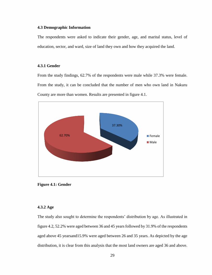
4.3.1 Gender

From the study findings, 62.7% of the respondents were male while 37.3% were female.

From the study, it can be concluded that the number of men who own land in Nakuru

County are more than women. Results are presented in figure 4.1.

Figure 4.1: Gender

4.3.2 Age

The study also sought to determine the respondents’ distribution by age. As illustrated in

figure 4.2, 52.2% were aged between 36 and 45 years followed by 31.9% of the respondents

aged above 45 yearsand15.9% were aged between 26 and 35 years. As depicted by the age

distribution, it is clear from this analysis that the most land owners are aged 36 and above.

37.30%

62.70% Female

Male

30

Figure 4.2: Age

4.3.3 Marital Status

The study also sought to establish the marital status of the respondents. 61.2% of the

respondents indicated that they were married while 22.4% were single. Those who

indicated that they were widows/widower and separated/divorced were represented by 9%

and 7.5% respectively. It is clear from the findings that, most of the respondents were from

stable families which are an indication of them being responsible.

26-35 Years 36-45 Years Above 45 Years

15.90%

52.20%

31.90%

31

Figure 4.3: Marital Status

4.3.4 Level of Education

The study further sought to establish the respondents’ level of education. From the findings,

55.2% of the respondents were College/university graduates, 28.4% of the respondents

were Secondary school leaverswhile16.4% of the respondents were primary school leavers.

From the study it can be deduced that majority of the respondents are College or university

level graduates.

Figure 4.3: Level of Education

22.40%

61.20%

9.00% 7.50%

16.40%

28.40%55.20%

Primary

Secondary

College/university

32

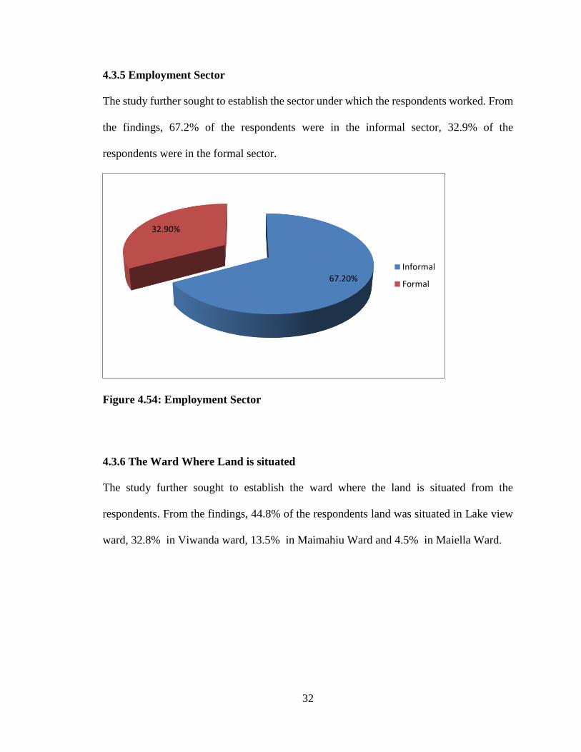
4.3.5 Employment Sector

The study further sought to establish the sector under which the respondents worked. From

the findings, 67.2% of the respondents were in the informal sector, 32.9% of the

respondents were in the formal sector.

Figure 4.54: Employment Sector

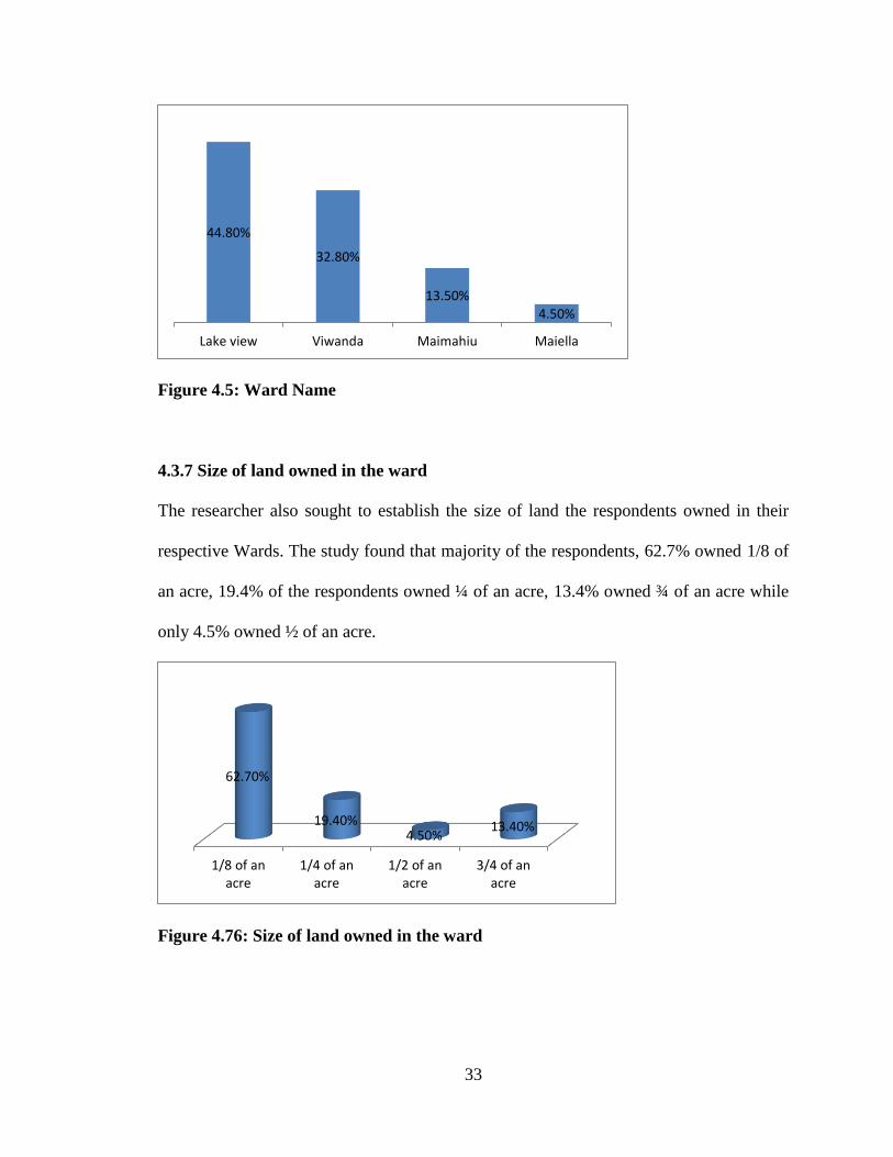
4.3.6 The Ward Where Land is situated

The study further sought to establish the ward where the land is situated from the

respondents. From the findings, 44.8% of the respondents land was situated in Lake view

ward, 32.8% in Viwanda ward, 13.5% in Maimahiu Ward and 4.5% in Maiella Ward.

67.20%

32.90%

Informal

Formal

33

Figure 4.5: Ward Name

4.3.7 Size of land owned in the ward

The researcher also sought to establish the size of land the respondents owned in their

respective Wards. The study found that majority of the respondents, 62.7% owned 1/8 of

an acre, 19.4% of the respondents owned ¼ of an acre, 13.4% owned ¾ of an acre while

only 4.5% owned ½ of an acre.

Figure 4.76: Size of land owned in the ward

44.80%

32.80%

13.50%4.50%

Lake view Viwanda Maimahiu Maiella

1/8 of anacre

1/4 of anacre

1/2 of anacre

3/4 of anacre

62.70%

19.40%4.50%

13.40%

34

4.3.8 Period when the owner acquired the land

The study further sought to establish when the respondents acquired the land. The findings

show that 34.3% acquired the land more than 10 years ago, 29.9% indicated that they

acquired the land between 1 and 5 years ago while 26.9% indicated between 6 and 9 years

ago. Lastly those who indicated to have acquired the land less than one year ago were 9%

of the entire respondents.

Figure 4.8: The duration the land was acquired

4.4 Descriptive Statistics

Descriptive statistics are the measures that describe the general nature of the data under

study. They define the nature of response from primary data and/or secondary data.

Descriptive statistics for this study were: mean and standard deviation. Graphic data

analysis was performed on the speculative investment demand, Interest rates, Proximity to

urban center and Real GDP. Descriptive statistics was carried out for different years as shown

below.

More than 10years ago

6-9 years ago 1-5 years ago Less than oneyear ago

34.30%

26.90%29.90%

9.00%

35

4.4.1 Speculative Investment Demand

The study sought to investigate the speculative investment demand by looking at the

percentage of people who indicated how they got the land, if through purchase, the price

they purchased it at, how the purchase was financed and what they intend to do with the

land and the current value of the land.

The study sought to establish how the land was financed. The results are illustrated in figure

4.9 below. From the results, 67.2% of the respondents indicated that they got the land

through purchase, 17.9% was through inheritance while 14.9% was through exchange.

Figure 4.7: Mode of Acquiring the Land

Purchase Inheritance Exchange

67.20%

17.90% 14.90%

36

4.4.1.1 Price of Land

Majority of the land owners indicated that the price of their land was estimated between

501,000 and 1,000,000 as indicated by 47.9% followed by 28.4% who owned land costing

between 100,000 and 250,000 and finally those who owned above 1m were 4.5%.

Figure 4.10: Price of land

4.4.1.2 How the purchase was financed

On how they purchased the land, 53.7% indicated the purchase was through personal

savings, 25.4% was through bank loan, 16.4% though Sacco loan while only 4.5% was

through mortgage.

28.40%19.50%

47.90%

4.50%

37

Figure 4.11: How the purchase was financed

4.4.1.3 What you intend to do with the land

The study also sought to establish what the respondents intended to do with their land as

illustrated from the results, 65.7% of the respondents indicated that they intended to

develop the land, 17.9% indicated their intention was to use the land for agriculture while

16.4% indicated their intention was to sell after a certain period of time.

Figure 4.12: What you intend to do with the land

Mortgage Bank loan Sacco loan Personalsavings

4.50%

25.40%16.40%

53.70%

Develop Use for agriculture Sell after a certainperiod

65.70%

17.90% 16.40%

38

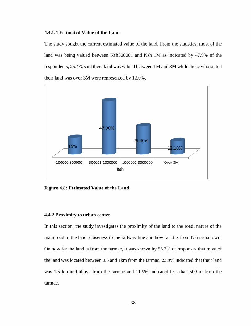
4.4.1.4 Estimated Value of the Land

The study sought the current estimated value of the land. From the statistics, most of the

land was being valued between Ksh500001 and Ksh 1M as indicated by 47.9% of the

respondents, 25.4% said there land was valued between 1M and 3M while those who stated

their land was over 3M were represented by 12.0%.

Figure 4.8: Estimated Value of the Land

4.4.2 Proximity to urban center

In this section, the study investigates the proximity of the land to the road, nature of the

main road to the land, closeness to the railway line and how far it is from Naivasha town.

On how far the land is from the tarmac, it was shown by 55.2% of responses that most of

the land was located between 0.5 and 1km from the tarmac. 23.9% indicated that their land

was 1.5 km and above from the tarmac and 11.9% indicated less than 500 m from the

tarmac.

100000-500000 500001-1000000 1000001-3000000 Over 3M

15%

47.90%

25.40%

12.10%

Ksh

39

4.4.2.1 Distance from the land to the road

Figure 4.14: Distance from the tarmac to your land

4.4.2.2 What is the nature of the main road to your Land

The respondents were asked to indicate the nature of the road to their land, as illustrated in

figure 4.15 below, 49.3% of the respondents indicated that they had all weather road to

their land and 31% indicated dusty road. The rest of the respondents 19.4% indicated that

they had tarmac road to their land.

Figure 4.15: The nature of the main road to your land

Less than500m

500-1km 1km-1.5km 1.5 km andabove

11.90%

55.20%

9.00%

23.90%

Tarmac All weather Dusty

19.40%

49.30%

31.30%

40

4.4.2.3 How near is the railway line to your land

On how near the railway line was to the land, majority of the respondents represented by

44.8% indicated that they were 1.5km and above from the railway line, 32.8% indicated

they were between 500m -1.5 km from the railway line, and lastly 9% were less than 500m

from the railway line.

Figure 4.9: Nearness of the railway line to your land

4.4.2.4 Nearness of Naivasha town from your land

The study further sought to establish how near the land is from Naivasha town. The results

show that most of the land was between 500m and 1.5km as illustrated by 50.7%, 35.9%

indicated between 1.6km and 5km while 13.5% showed their land was over 5km from

Naivasha town.

Less than500m

500-1km 1km-1.5km 1.5 km andabove

9.00%

32.80%

13.40%

44.80%

41

Figure 4.10: Nearness of Naivasha town from your land

4.4.3 Real GDP

The table shows the Real GDP as measured using the figures provided by KNBS. The

results show that, the Kenya’s Gross domestic product has been steadily growing from

2012 to 2016.This shows that the sectors such as: agriculture, mining and quarrying,

manufacturing, electricity and water supply, construction industry, wholesale and retail

trade, accommodation and food services, transport and storage information, and

communication which are the key determinants of the real GDP have been recording

growth over the period.

Table 4.2: Real GDP (KSh Million)

Year 2012 2013 2014 2015 2016

Quarter 1 1,035,113 1,142,221 1,300,095 1,506,384 1,626,767

2 1,050,755 1,168,578 1,323,824 1,536,585 1,811,965

3 1,065,056 1,205,069 1,366,620 1,580,496 1,853,017

4 1,119,436 1,241,846 1,426,641 1,653,299 1,883,949

Average 1,067,590 1,189,429 1,354,295 1,569,191 1,793,925

50.70%

35.90%

13.50%

500-1.5km

1.6-5km

Over 5km

42

4.4.4 Lending Interest Rate

The study sought to establish central banks’ lending rates from 2012 to 2016. From the

statistics obtained from the CBK, CBK lending rates have been steady over the last three

years except in 2012 when it stood at 19.65%. The year 2015 recorded the lowest lending

rates. However, going by the quarters, CBK issued the lowest lending rates to her

customers in the last quarter of 2016 which were 13.86, 13.73, 13.67 and 13.66 in the

months of September, October, November and December. From these statistics, the study

can deduce that since the capping of interest rates charged by commercial banks to their

customers, the CBK on her part has been able to offer favorable rates to the commercial

banks hence creating a favorable business environment for other people to get loans from

commercial banks at favorable interest rates.

Table 4.3: Lending Interest Rate from CBK in %

2012 2013 2014 2015 2016

Jan 19.54 18.13 17.03 15.93 18

Feb 20.28 17.84 17.06 15.47 17.91

Mar 20.34 17.73 16.91 15.46 17.87

Apr 20.22 17.87 16.7 15.4 18.04

May 20.12 17.45 16.97 15.26 18.22

Jun 20.3 16.97 16.36 16.06 18.18

Jul 20.15 17.02 16.91 15.75 18.1

Aug 20.13 16.96 16.26 15.68 17.66

Sep 19.73 16.86 16.04 16.82 13.86

Oct 19.04 17 16 16.58 13.73

Nov 17.78 16.89 15.94 17.16 13.67

Dec 18.15 16.99 15.99 18.3 13.66

Average Lending

Rate per year

19.65 17.31 16.51 16.16 16.58

43

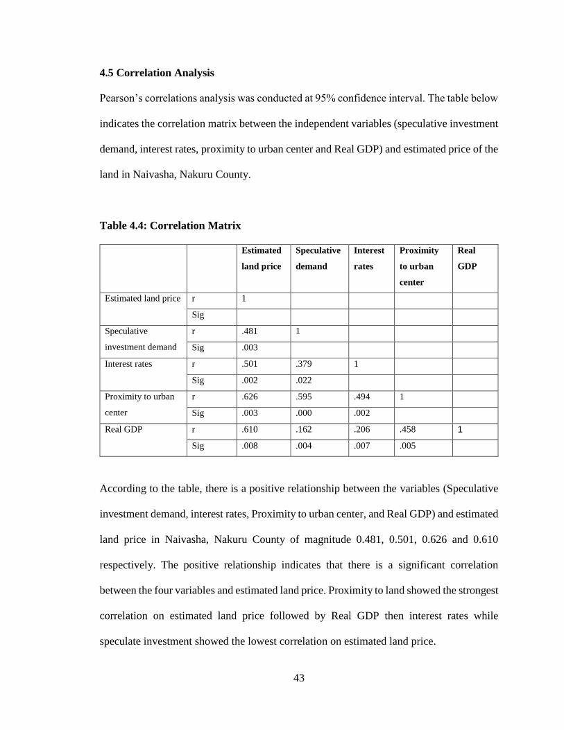
4.5 Correlation Analysis

Pearson’s correlations analysis was conducted at 95% confidence interval. The table below

indicates the correlation matrix between the independent variables (speculative investment

demand, interest rates, proximity to urban center and Real GDP) and estimated price of the

land in Naivasha, Nakuru County.

Table 4.4: Correlation Matrix

Estimated

land price

Speculative

demand

Interest

rates

Proximity

to urban

center

Real

GDP

Estimated land price r 1

Sig

Speculative

investment demand

r .481 1

Sig .003

Interest rates r .501 .379 1

Sig .002 .022

Proximity to urban

center

r .626 .595 .494 1

Sig .003 .000 .002

Real GDP r .610 .162 .206 .458 1

Sig .008 .004 .007 .005

According to the table, there is a positive relationship between the variables (Speculative

investment demand, interest rates, Proximity to urban center, and Real GDP) and estimated

land price in Naivasha, Nakuru County of magnitude 0.481, 0.501, 0.626 and 0.610

respectively. The positive relationship indicates that there is a significant correlation

between the four variables and estimated land price. Proximity to land showed the strongest

correlation on estimated land price followed by Real GDP then interest rates while

speculate investment showed the lowest correlation on estimated land price.

44

4.6 Regression Analysis

Having carried out the descriptive statistics the study employed inferential statistics so as

to draw conclusions and recommendations.

4.6.1 Cross tabulation of Land price against estimated current price

The study conducted a cross tabulation of the price of land at the time of acquisition and

the estimated value at the moment.

Table 4.5: Cross tabulation of Price of land at the time of acquisition versus

estimated value of the land

Price of

land at the

time of

acquisition

x Ksh

1000

Estimated valued of the land x Ksh10000 Total

45 50 60 70 75 80 85 90 100 120 150 200 500

100.00 3 0 0 0 0 0 0 0 0 0 0 0 0 3

150.00 0 3 3 2 0 0 0 0 0 0 0 0 0 8

200.00 0 0 0 0 0 0 0 0 3 0 0 0 0 3

250.00 0 0 0 0 0 0 0 0 0 3 2 0 0 5

300.00 0 0 0 0 0 3 3 0 0 0 0 0 0 6

350.00 0 2 0 0 0 0 0 0 0 0 0 0 0 2

450.00 0 0 0 0 2 0 0 0 0 0 0 0 0 2

500.00 0 0 0 0 0 0 0 0 0 0 0 3 0 3

650.00 0 0 0 0 0 0 0 0 2 0 0 0 0 2

850.00 0 0 0 0 0 0 0 2 2 0 0 0 0 4

1000.00 0 0 0 0 0 0 0 0 0 4 2 0 0 6

3000.00 0 0 0 0 0 0 0 0 0 0 0 0 3 3

Total 3 5 3 2 2 3 3 2 7 7 4 3 3 47

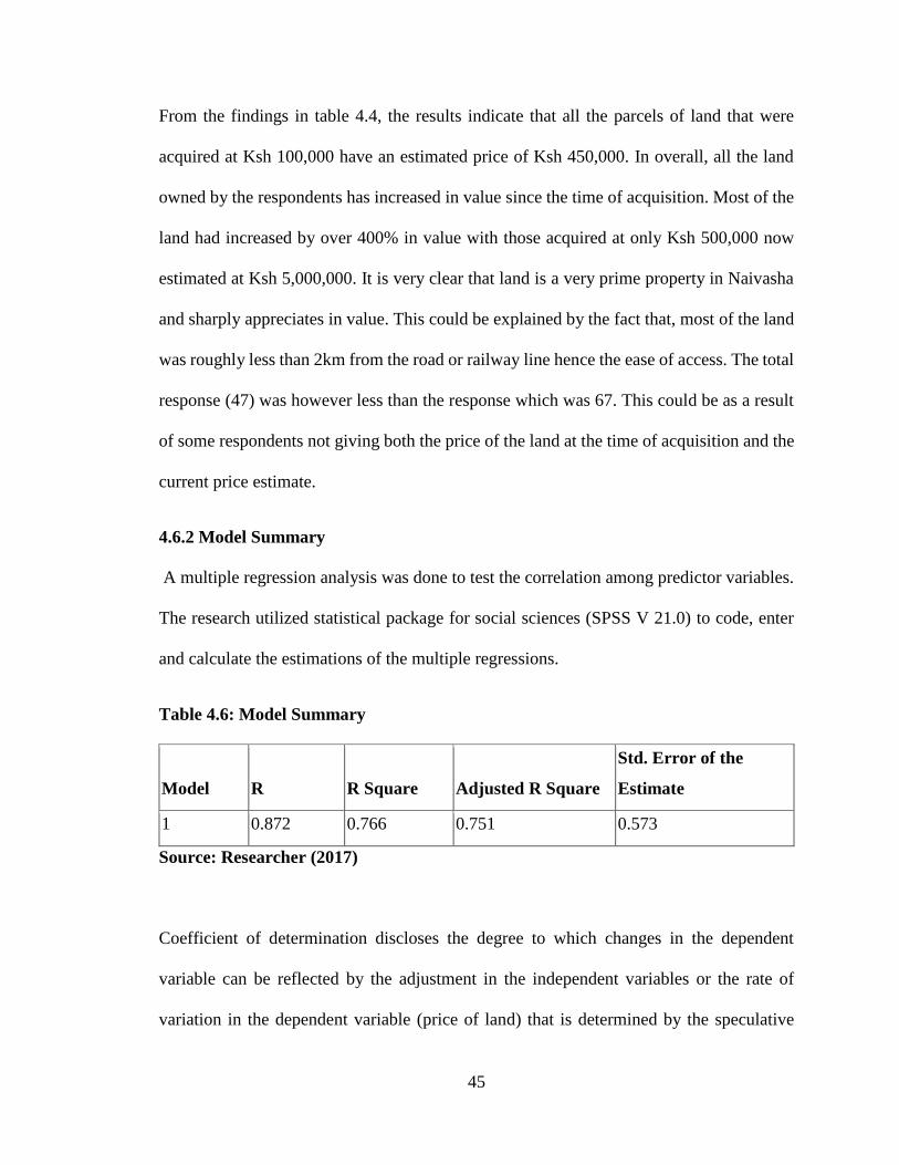
45

From the findings in table 4.4, the results indicate that all the parcels of land that were

acquired at Ksh 100,000 have an estimated price of Ksh 450,000. In overall, all the land

owned by the respondents has increased in value since the time of acquisition. Most of the

land had increased by over 400% in value with those acquired at only Ksh 500,000 now

estimated at Ksh 5,000,000. It is very clear that land is a very prime property in Naivasha

and sharply appreciates in value. This could be explained by the fact that, most of the land

was roughly less than 2km from the road or railway line hence the ease of access. The total

response (47) was however less than the response which was 67. This could be as a result

of some respondents not giving both the price of the land at the time of acquisition and the

current price estimate.

4.6.2 Model Summary

A multiple regression analysis was done to test the correlation among predictor variables.

The research utilized statistical package for social sciences (SPSS V 21.0) to code, enter

and calculate the estimations of the multiple regressions.

Table 4.6: Model Summary

Model R R Square Adjusted R Square

Std. Error of the

Estimate

1 0.872 0.766 0.751 0.573

Source: Researcher (2017)

Coefficient of determination discloses the degree to which changes in the dependent

variable can be reflected by the adjustment in the independent variables or the rate of

variation in the dependent variable (price of land) that is determined by the speculative

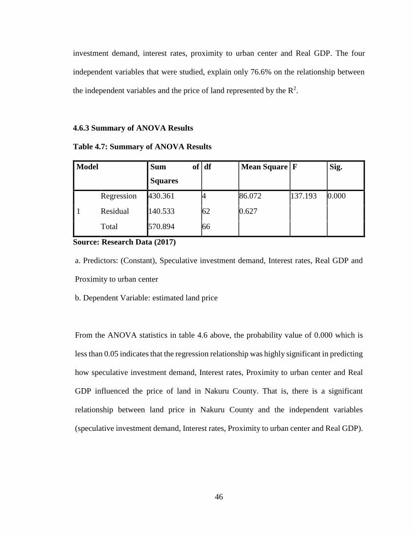
46

investment demand, interest rates, proximity to urban center and Real GDP. The four

independent variables that were studied, explain only 76.6% on the relationship between

the independent variables and the price of land represented by the R2.

4.6.3 Summary of ANOVA Results

Table 4.7: Summary of ANOVA Results

Model Sum of

Squares

df Mean Square F Sig.

1

Regression 430.361 4 86.072 137.193 0.000

Residual 140.533 62 0.627

Total 570.894 66

Source: Research Data (2017)

a. Predictors: (Constant), Speculative investment demand, Interest rates, Real GDP and

Proximity to urban center

b. Dependent Variable: estimated land price

From the ANOVA statistics in table 4.6 above, the probability value of 0.000 which is

less than 0.05 indicates that the regression relationship was highly significant in predicting

how speculative investment demand, Interest rates, Proximity to urban center and Real

GDP influenced the price of land in Nakuru County. That is, there is a significant

relationship between land price in Nakuru County and the independent variables

(speculative investment demand, Interest rates, Proximity to urban center and Real GDP).

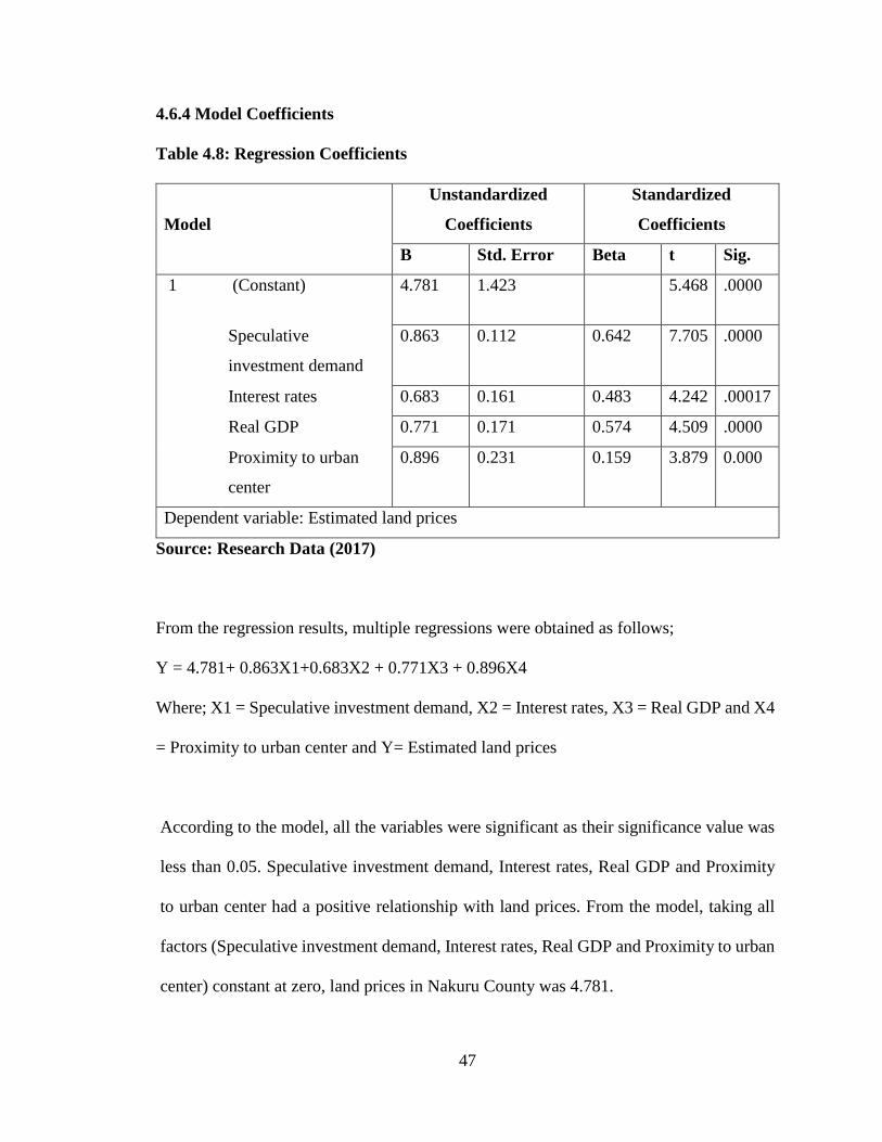
47

4.6.4 Model Coefficients

Table 4.8: Regression Coefficients

Model

Unstandardized

Coefficients

Standardized

Coefficients

B Std. Error Beta t Sig.

1 (Constant) 4.781 1.423 5.468 .0000

Speculative

investment demand

0.863 0.112 0.642 7.705 .0000

Interest rates 0.683 0.161 0.483 4.242 .00017

Real GDP 0.771 0.171 0.574 4.509 .0000

Proximity to urban

center

0.896 0.231 0.159 3.879 0.000

Dependent variable: Estimated land prices

Source: Research Data (2017)

From the regression results, multiple regressions were obtained as follows;

Y = 4.781+ 0.863X1+0.683X2 + 0.771X3 + 0.896X4

Where; X1 = Speculative investment demand, X2 = Interest rates, X3 = Real GDP and X4

= Proximity to urban center and Y= Estimated land prices

According to the model, all the variables were significant as their significance value was

less than 0.05. Speculative investment demand, Interest rates, Real GDP and Proximity

to urban center had a positive relationship with land prices. From the model, taking all

factors (Speculative investment demand, Interest rates, Real GDP and Proximity to urban

center) constant at zero, land prices in Nakuru County was 4.781.

48

The regression results also shows that speculative investment demand had positive and

significant relationship with land prices (β1 =0.863, P= 0.000).

The study also found that interest rates had positive and significant relationship with land

prices (β2 =0.683, P=0.000).

The study also found that Real GDP had positive and significant relationship with land

prices (β3 = 0.771, P=.039).

The study further found that Proximity to urban center had positive and significant

relationship land prices (β2 =0.896, P=0.000). This infers that Proximity to urban center

contributed most to the land prices followed by Speculative investment demand then Real

GDP while Interest rates had the least significant effect on the land prices.

4.7 Discussion of Findings

The findings of this study where the four variables (Speculative investment demand,

Interest rates, Real GDP and Proximity to urban center) have a significant positive

relationship with the independent variable are similar to studies done both internationally

and locally. Li, (2009) found out that GDP growth strongly affects land prices which are

similar to the results of this study. Li and Chang, (2012) in their study also find that real

estate prices are affected by both institutional and economic factors and from this

conclusion the economic factors include GDP growth and interest rates which agrees with

what the researcher has found out. Marete (2011) in her study found out that location of

real estate had a significant positive relationship with the price of real estate property. In

this study it has also been proven that proximity to urban center has a similar effect.

49

CHAPTER FIVE

SUMMARY OF FINDINGS, CONCLUSIONS AND

RECOMMENDATIONS

5.1 Introduction

This chapter presents the summary of the findings from chapter four, and it also gives the

discussions, conclusions and recommendations of the study based on the objectives of the

study. The objective of this study was to find out the factors influencing the price of land

in Nakuru County.

5.2 Summary of Findings

The objective of the study was to find out the factors influencing the price of land in Nakuru

county. The study found that all the land owned by the respondents increased in value since

the time of acquisition. Most of the land had increased by over 400% in value. The

regression relationship was highly significant in predicting how speculative investment

demand, Interest rates, Proximity to urban center and Real GDP influenced the price of

land in Nakuru County. The four independent variables that were studied, explained only

76.6% on the relationship between the independent variables and the price of land

represented by the R2. That is, there was a significant positive relationship between land

price in Nakuru County and the independent variables (speculative investment demand,

Interest rates, Proximity to urban center and Real GDP). According to the model, all the

variables were significant as their significance value was less than 0.05. From the model,

taking all factors (Speculative investment demand, Interest rates, Real GDP and Proximity

to urban center) constant at zero, land prices in Nakuru County was 4.781.

50

5.3 Conclusion of the Study and Policy Recommendation

From the findings of this study it is clearly evident that land price in Nakuru county is

influenced by all the dependent variables which include: speculative investment demand,

Interest rates, Real GDP and Proximity to urban center. Land price has been steadily

increasing over the period of study and this is explained by the positive relationship with

speculative investment demand which had a correlation of 0.481, interest rates with a

correlation of 0.481, proximity to urban center 0.626 and finally real GDP with 0.610. The

objectives of the study were therefore met.

It is recommended that policy makers in government look for ways of increasing the

growth of GDP so that majority of people can afford to buy land. The lending interest rate

should also be reduced further so that people can get loans that are cheaper and thus afford

to buy land. Dusty and murram roads should have tarmac to improve transportation and

also the value of the land.

5.4 Limitations of the study

The researcher was faced with several limitations which are pertinent to this study. The

time for carrying out the study was not adequate therefore the sample was small hence

introducing sampling error. The answers given in the questionnaires are solely based on

the honesty of the respondents. The researcher also faced a financial challenge and

therefore wasn’t able to carry out a larger sampling size that would have minimized the

sampling error.

51

5.5 Suggestions for Further Research

This study investigated the factors influencing the price of land in Nakuru County. The

researcher suggests that similar studies be conducted on other factors apart from the four

that are likely to determine the price of land in the county. Studies should also be done to

determine factors influencing the price of land in other counties in Kenya so that a

generalization can be made on the factors influencing the price of land in Kenya.

REFERENCES

Achen, C.H. (1982). Interpreting and using regression, Sage Publications, Newbury Park,

CA.

52

Allen, M. J., & Yen, W.M. (1979). Introduction to Measurement Theory. Monterey:

Brooks/Cole.

Altuzarra, A., & Esteban, M. (2011).Land prices and housing prices: the case of Spain.

Journal of Housing and the Built Environment, 26(4), 397-409.

Arnold, M. A. (1992). The principal-agent relationship in real estate brokerage services.

Journal of the American Real Estate and Urban Economics Association, 20, (1)

89-106.

Baker, M., & Wurgler, J. (2006). Investor Sentiment and the Cross-Section of Stock

Returns, Journal of Finance, 61(4), 1645-1680.

Balkin, D., & Gomez, M.(1992). Determinants of faculty pay - an agency theory

perspective. The Academy of Management Journal, 35(5), 921 -955.

Brueggeman, W. B., & Fisher, J.D. (2011). Real estate finance and

investments.14thEd.Newyork: McGraw- Hill.

Chau, K.W., Wong S.K., &Yiu, C.Y. (2003). Price discovery function of forward contracts

in the real estate market: an empirical test. Journal of financial management of

property and construction, 8(3), 129-137.

Capozza, D.R., Hendershott, P.H., Mack, C., & Mayer C. J. (2004). Determinants of real

house price dynamics. Journal of real estate economics. 32(2), 29-79.

Ding, J. (2014). An Empirical Analysis of Factors Affecting Chinese Real Estate Prices,

Unpublished masters project. School of Economic and Management, Central

China Normal University.

Eisenhardt, K. M. (1989). Agency theory: an assessment and review. Academy of

Management Review, 14(1).

Gay, L., &Liu, H. (1992). Educational Research: Competency for analysis and

Application. USA: Snippet View.

Gitonga, A. (2014). Naivasha welcomes its first gated estate. Retrieved on July 15,

2017,fromstandardnewspaperwebsite:http://www.standardmedia.co.ke/business/a

rticle/2000138397/Naivasha-welcomes-itsfirst-gated-estate.

Goslings, J.H.,& Petri, V.L. (1992).The Role of Real Estate in Efficient Investment

Portfolios, Journal of property valuation and investment,10(1), 405 – 412.

53

Ho,W.K. & Ganesan, S.(1998). On land supply and the price of residential housing.

Netherlands Journal of Housing and the Built Environment, 13(4), 439-452.

Karoki R.W. (2013). Determinants of residential real estate prices in Kenya, unpublished

MBA project 2013.

Kombo, D.K. and Tromp D.L.A. (2006).Proposal and thesis writing an introduction.

Makuyu: Pauline’s Publications Africa.

Kothari, C.K. (2004).(2nded.). Research methodology: methods and techniques. New

Delhi: international (p) ltd.

Lancaster, K. J. (1966). A New Approach to Consumer Theory, Journal of Political

Economy, 74, 132-157.

Levin, E.J., &R.E. Wright (1997).Speculation in the Housing Market. Urban Studies.

34,(9), 1419-1437.

Li, L. (2015). Prices and Bubbles: Factors Affecting the Chinese Real Estate Market.

Unpublished Masters Project. Master Program in International Economics with a

focus on China, Lund University, Sweden.

Li, J., & Chiang, Y. (2012).What pushes up China’s real estate price? International Journal

of Housing Markets and Analysis, 5(2),161 – 176.

Li, L.(2009). Land price changes in the evolving land market in Beijing. Property

Management, 27 (2), 91 – 108.

Lieser, K. & Groh, A.P. (2011).The Determinants of International Commercial Real Estate

Investments. Journal of political economics, 89(3),234-285.

Markowitz H.M. (1999) The early history of portfolio theory: 1660-1960.Financial

analysts journal,55(4) 5-16.

Marete, D.K.(2011). The determinants of real estate property prices: the case of Kiambu

municipality in Kenya Unpublished MBA project 2011

Malpezzi, S. & Watcher, S. (2005) The roles of speculation in real estate cycles. Journal

or real estate literature, 13 (2), 141 - 164

McEachern, W. A. (2011). Economics: A Contemporary Introduction, New York: Cengage

Learning.

54

Muhoro, M. (2006). Eveready cancels plan to build Nakuru mall on glut fears. Retrieved

on June 18, 2017, from construction business review website: http://www.

Constructionkenya.com/3557/Eveready-Nakuru-factory-land/

Mugenda, O. M., &Mugenda, A. G. (2003).Quantitative and Qualitative Approaches (2nd

ed.). Nairobi: Acts Press.

Neuman,W.L. (2010) .Social Research Methods: Qualitative & Quantitative Approaches(7

th ed.). Ontario Canada: Pearson Education.

Omboi, B.M & Kegige, A. M. (2011).Factors influencing real estate property prices a

survey of real estates in Meru Municipality, Kenya. Journal of Economics and

Sustainable 2(4),34-54.

Pavlov,A., & Wachter, S.(2010). Subprime lending and real estate prices. Journal of real

estate economics,39(1),1-17.

Pagourtzi, E., Assimakopoulos, A., Hatzichristos, T., &French, N. (2003).Real estate

appraisal: a review of valuation methods, Journal of Property Investment &

Finance, 21 (4), 383 – 401.

Rosen, S. (1974).Hedonic prices and implicit markets: product differentiation in pure

competition. Journal of Political Economy, 82(1), 34-55.

Statman, M.(1999). Behavioral finance: past battles and future engagements. Financial

analyst journal, 55(6), 534 -576

55

APPENDICES

APPENDIX I: QUESTIONNAIRE

Introduction

The objective of this research is to establish the factors that influence real estate property

prices in Nakuru County in Kenya. Please answer the questions in this questionnaire by

inserting "X" in the boxes provided or by filling out the spaces provided as briefly as

possible.

SECTION A: PERSONAL INFORMATION

Please tick (√) the option that corresponds to your answer in each of the following:

1. Gender

(a) Female ( ) (b) Male ( )

2. What is your age?

(a) Below 25 ( ) (b) 26 – 35 ( )

(c) 36 -45 ( ) (d) Above 45 ( )

3. Marital status

(a) Single ( ) (b) Married ( )

(c) Widow/widower ( ) (d) Separated/Divorced ( )

4. What is your highest level of education?

(a) Non-formal ( ) (b) Primary ( )

(c) Secondary ( ) (d) College/University ( )

5. Do you work in formal or informal sector?..................

6. In which ward of Naivasha Sub County do you live?

(a) Lakeview ( ) (b) Viwanda ( )

(f) Mai mahiu( ) (g) Maiella ( )

7. What size of land do you own within the ward?

(a) 1/8 of an acre ( ) (b) ¼ of an acre ( )

(c) ½ of an acre ( ) (d) ¾ of an acre ( )

(e) 1 acre ( ) (f) Others (specify)………………………

8. When did you acquire the land?

(a) More than 10 years ago ( ) (b) (6-9) years ago ( )

(c) (1-5) years ago ( ) (d) Less than one year ago ( )

56

SECTION B: SPECULATIVE INVESTMENT DEMAND

9. How did you acquire the land?

(a) Through purchase ( ) (b) Through inheritance ( )

(c) Through exchange ( ) (d) Others (specify)…………………….

10. If (in 9 above) was through purchase, what was the price? Please state.

Ksh………………………..

11. How did you finance the purchase?

(a) Mortgage ( ) (b) Bank Loan ( )

(c) Sacco Loan ( ) (d) Personal savings ( )

(e) Others (specify)……………………………………….

12. What do you intend to do with the land?

(a) Develop ( ) (b) Use for agriculture ( )

(c) Sell after a certain period ( ) (d) Others (specify)…………….

13. In Your own estimate, what is the value of your piece of land today?

Ksh……………………………………..

SECTION C: PROXIMITY TO URBAN CENTER

18. How far from the tarmac is your land?

(a) Less than 500m ( ) (b) 500m – 1 Km ( )

( ) 1 Km – 1.5 Km ( ) (d) 1.5 km and above ( )

19. What is the nature of the main road to your land?

(a) Tarmac ( ) (b) All weather ( )

(c) Dusty ( )

20. How near is a railway line to your land?

(a) Less than 500m ( ) (b) 500m – 1 Km ( )

(c) 1 Km – 1.5 Km ( ) (d) 1.5 km and above ( )

21. How far is Naivasha town from your land?......................................

THANK YOU FOR YOUR CO-OPERATION.

57

APPENDIX II: GDP IN MILLIONS

Year Quarter

1 2 3 4

2012 1,035,113 1,050,755 1,065,056 1,119,436 1,067,590

2013 1,142,221 1,168,578 1,205,069 1,241,846 1,189,429

2014 1,300,095 1,323,824 1,366,620 1,426,641 1,354,295

2015 1,506,384 1,536,585 1,580,496 1,653,299 1,569,191

2016 1,626,767 1,811,965 1,853,017 1,883,949 1,793,925