Embed Size (px)
Citation preview

وزارة التعليم العالي والبحث العلمي
ANNABA- BADJI MOKHTAR باجي مختار جامعة
UNIVERSITY -عنابة- - UNIVERSITE BADJI MOKHTAR
ANNABA
Faculté des Sciences Département de Mathématiques
THESE
Présentée en vue de l'obtention du diplôme de DOCTORAT EN MATHEMATIQUES
Option: Control Optimal Stochastique
Solution process of a class of differential equation using Homotopy
Analysis Wiener-Hermite Expansion and Perturbation technique
Par
BOUKEHILA Ahcene
Directeur de Thèse: BENMOSTEFA FATIMA ZOHRA MCA U.B.M. ANNABA
Devant le Jury
PRESIDENT BENCHETTAH Azzedine Pr U.B.M. ANNABA
EXAMINATEUR AISSAOUI Mohamed Zine MCA U. GUELMA
EXAMINATEUR BOUTABIA Hacène Pr U.B.M. ANNABA
EXAMINATEUR ELLAGGOUNE Fateh MCA U. GUELMA
EXAMINATEUR GUESMIA Amar MCA U. SKIKDA
Année Universitaire 2014/2015

i
ملخص
هو حول تطبيق طريقة جديدة للدكتوراه إن موضوع الدراسة التي قدمت في هذه األطروحة
طريقة هرميت باالرتياب وتسمى -من الطريقة الهوموتوبية للتحليل مع طريقة نشر وينير تتكون
على صنف من بنجاح هرميت باالرتياب. طبقت هذه الطريقة-الهوموتوبي للتحليل نشر وينير
دالت التفاضلية العشوائية إلثبات أن الحل المتمثل في األمل الرياضي والتباين أن كال منهما المعا
متقارب بواسطة تطبيق هذه الطريقة.
استعمال الطريقة الهوموتوبية لالرتياب وتفاديالهدف من تطبيق هذة الريق الجديدة هو لتجاوز
.الطريقة الهوموتوبية للتحليلالتي ال تضمن تقارب الحل وكذلك أنها حالة خاصة من
;هرميت باالرتياب -طريقة نشر وينير ;من الطريقة الهوموتوبية للتحليل :الكلمات المفتاحية
;المعادالت التفاضلية العشوائية ;هرميت باالرتياب-طريقة الهوموتوبي للتحليل نشر وينير
.معادلة النجوفين

Abstract
In this thesis, we present a new method based on Wiener Hermite Expansion and
Perturbation technique or WHEP linked to Homotopy Analysis Method or HAM and it is
called HAMWHEP technique and then apply it for solving a class of dierential equation.
Using the Homotopy Perturbation Method linked to WHEP in [6] may lead to divergence,
there is absolutely no guarantee that perturbation methods result in a convergent solution.
This disadvantage is overcome by using the Homotopy Analysis Method (HAM) linked to
WHEP or (HAM WHEP) technique which guarantees the convergence of the solution.
Keywords : Wiener Process, Wiener Hermite Expansion and Perturbation technique,
Homotopy Perturbation Method, Homotopy Analysis Method, HAM WHEP technique,
Langevin Equation, Stochastic dierential Equation, Initial and Boundary Value Pro-
blems.
Résumé
Dans cette Thèse on présente une nouvelle methode basée sur le développement de
Wiener Hermite et le méthode perturbative oubien WHEP liée à la méthode d'Homotopy
et d'analyse, et l'appliquée pour résoudre une classe d'équation diérentielle.
l'utilisation de la méthode WHEP liée à la méthode d'Homotopy et de Perturbation dans
[6] peut conduire à divergence de la solution. cet disaventage est surmonter en utilisant
la méthode WHEP liée à la méthode d'Homotopy et d'analyse qui assure la convergence
de la solution
Mots clés : Processus de Wiener, Développement de Wiener Hermite et la méthode
perturbative, la méthode d'Homotopy et de Perturbation, la méthode d'Homotopy et
d'analyse, l'Equation de Langevin, Equation Diérentielle Stochastique, Problem Initial,
Problem aux Limites.
ii

Dédicace
A ma familleet mes parents
à la mémoire duProfesseur Magdy El Tawil
qui est décédé en 2013.
iii

Remerciements
Cette thèse n'aurait jamais été possible sans la conance, la patience de mon super-
viseur Benmostefa Fatima Zohra je voudrais la remercier chaleureusement. Je voudrais
aussi la remercier pour les conseils que m'a guidé tout au long de la production de cette
thèse. En fait, je ne peux pas exprimer ma gratitude en quelques lignes.
Professeur BENCHETTAH Azzedine m'a fait le grand honneur de présider le jury. Je le
remercie très vivement.
Je remercie les professeurs BOUTABIA Hacene, AISSAOUI Zine, ELLAGGOUNE Fateh
et GUESMIA Amar pour me donner l'honneur d'être examinateurs de cette thèse.
Enn, je tiens à orir mes plus sincères remerciements à ma famille, mes parents, frères
et mes amis pour leur soutien constant tout au long de la années de la thèse.
iv

Liste des Figures
2.3 Dierentes corrections de l'espérance, Homotopy WHEP n=2 . . . . . . . . . . . . . . . . 19
2.3 Dierentes corrections de la variance, Homotopy WHEP, n=2 . . . . . . . . . . . . . . . . 19
2.3Deuxième correction de l'espérance, Homotopy WHEP n=2, . . . . . . . . . . . . . . . . . 20
2.3Deuxième correction de la variance, Homotopy WHEP n=2, . . . . . . . . . . . . . . . . . .20
3.1.3 ~-courbe de l'espérance obtenue par la 4ème appr de HAM . . . . . . . . . . . . . . . . 26
3.2 ~-courbe de la variance obtenue par la 4ème appr de HAM . . . . . . . . . . . . . . . . . . 26
3.1.4 ~-courbe de l'espérance obtenue par la 6ème appr de HAM WHEP n=2 . . . 27
3.4 ~-courbe de la variance obtenue par la 5ème appr de HAM WHEP n=2 . . . . . 28
3.5 ~-courbe de l'espérance obtenue par la 4ème appr de HAM WHEP n=3 . . . . . 28
3.6 ~-courbe de la variance obtenue par la 4ème appr de HAM WHEP n=3 . . . . . 29
4.1 ~-courbe de l'espérance obtenue par la 5ème appr de HAM WHEP n=2 . . . . . 33
4.2 ~-courbe de la variance obtenue par la 5ème appr de HAM WHEP n=2 . . . . . 33
4.3 ~-courbe de l'espérance obtenue par la 5ème appr de HAM WHEP n=3 . . . . . 34
4.4 ~-courbe de la variance obtenue par la 5ème appr de HAM WHEP n=3 . . . . . 34
v

Liste des of Symboles
v : variance
u : espérance
W (t) : processus de wiener
dW (t) ; est la dérivée du mouvement Brownien ,i.e,n(t).
f(t), t ≥ 0 : est un processus stochastique dont les trajectoires sont p.s. continues et il
est adapté à la ltration Ft
f ∈ M2 :Intégrale d'Ito I(f) existe, et E(∫∞0
|f(t)|2dt) < ∞
f ∈ M2T : Intégrale d'Ito IT (f) existe, et E(
∫ T
0|f(t)|2dt) < ∞
ξ(t), t ≥ 0 est un processus Ito dont les trajectoires continues p.s et
ξ(t) = ξ(0) +∫ T
0a(t)dt+
∫ T
0b(t)dW (t)a.s.
The space M2 : se compose de tous les processus stochastiques progressivement
mesurable f(t) tel que E(∫∞0
|f(t)|2dt) < ∞
l'espace M2T : se compose de tous les processus stochastiques progressivement mesurable
f(t) tel que E(∫ T
0|f(t)|2dt) < ∞.
~ : un paramètre à régler et de contrôler la zone de convergence et le taux de
convergence de la série de la solution.
WHEP technique : le développement de Wiener Hermite et la technique de la
vi

perturbation.
HPM : la Méthode de la Perturbation Homotopique.
HAM : la Méthode de l'Analyse Homotopique.
HAM WHEP technique :la méthode de l'Analyse Homotopique liée au développement
de Wiener Hermite et la technique de la perturbation
vii

Sommaire
Liste des Figures . . . . . . . . . . . . . . . . . . . . . . . . . . . . . . . . . . . . . . . . . . . . . . . . . . . . . . . . . . . . . .vi
Liste des Symboles . . . . . . . . . . . . . . . . . . . . . . . . . . . . . . . . . . . . . . . . . . . . . . . . . . . . . . . . . . .vii
Introduction . . . . . . . . . . . . . . . . . . . . . . . . . . . . . . . . . . . . . . . . . . . . . . . . . . . . . . . . . . . . . . . . . . . .3
1 Notes sur les équations diérentielles stochastiques . . . . . . . . . . . . . . . . . . . . . . 5
1.1 Dénitions et propriétés de base des processus de Wiener . . . . . . . . . . . . . . . . . .5
1.2 Calcul stochastique de Ito . . . . . . . . . . . . . . . . . . . . . . . . . . . . . . . . . . . . . . . . . . . . . . . . .6
1.3. Propriétés de l'intégrale stochastique . . . . . . . . . . . . . . . . . . . . . . . . . . . . . . . . . . . . . 9
1.4 Calcul stochastique et la Formule de Ito . . . . . . . . . . . . . . . . . . . . . . . . . . . . . . . . .10
1.5 Equations diérentielles stochastiques . . . . . . . . . . . . . . . . . . . . . . . . . . . . . . . . . . . .11
2 La Technique de Homotopie WHEP . . . . . . . . . . . . . . . . . . . . . . . . . . . . . . . . . . . . . 13
2.1 Le développement de Wiener Hermite et la technique de la perturbation. .13
2.2 La méthode de Homotopie et la Perturbation . . . . . . . . . . . . . . . . . . . . . . . . . . . .16
2.3 La technique de Homotopie WHEP . . . . . . . . . . . . . . . . . . . . . . . . . . . . . . . . . . . . . 17
3 Résolution d'un problème de valeur initiale par HAM WHEP . . . . . . . .21
3.1 La méthode de l'Analyse Homotopique. . . . . . . . . . . . . . . . . . . . . . . . . . . . . . . . . . .21
3.2 La résolution de l'équation de Langevin par la technique de WHEP . . . . . 24
3.3 La résolution de l'équation de Langevin par l'Analyse Homotopique . . . . . . 25
3.4 La résolution de l'équation de Langevin par la technique de HAM WHEP 27
4 Résolution d'un problème aux limites par la technique de HAMWHEP 30
1

4.1 Résoudre l'EDS de diuson non linéaire en utilisant HAM WHEP. . . . . . . .30
Conclusion
Bibliographie
Appendice
2

Introdution
L'étude de solutions aléatoires des équations aux dérivées partielles était initié par
Kampe de Fériet en 1955 [ 26 ] . Dans son étude précieuse sur la théorie des équations
aléatoires , Bharucha - Reid a montré comment un équation de la chaleur stochastique de
type Cauchy peut être résolu en utilisant la la théorie des intégrales stochastiques [ 27 ] .
En 1973 , Lo Dato [ 28 ] a estimé le champ de vitesse stochastique et l'équation de Navier
Stokes et discuté des problèmes mathématiques qui lui sont associés . Becus [ 29 ] introduit
une solution générale au problème de conduction de chaleur avec un terme source aléatoire
et les conditions initiales et aux limites aléatoires . beaucoup auteurs ont étudié l'équation
de diusion stochastique sous diérents points de vue [ 5-11 ] . Récemment, M. A. El -
Tawil utilisé le Wiener L'expansion Hermite avec la théorie de la perturbation ( WHEP
) technique pour résoudre une équation de diusion non linéaire stochastique perturbée
[ 4 ] . La technique a ensuite été mis au point pour être appliqué sur le non- perturbée
équations diérentielles à l'aide de la méthode de perturbation lié Homotopy Wiener
Hermite technique développement de perturbation et il est appelé Homotopy WHEP [ 3 ].
Cependant, comme mentionné S.J. Liao [ 19 ] , la méthode de Perturbation Homotopique
( HPM ) n'est qu'un cas particulier de la méthode d'Analyse Homotopique ( HAM) .
La diérence est que , le HPM a dû utiliser une assez bonne estimation initiale, mais ce
n'est pas absolument nécessaire pour la méthode HAM . C'est important parce que la
HAM utilise un paramètre de contrôler pour garantir la convergence de l'approximation
de la série sur un intervalle donné. Ainsi, la méthode d'Analyse Homotopique (HAM )
est plus générale . En 2010, MA El-Tawil et NA Al-Mulla [6] ont utilisé le HPM lié à
la technique WHEP pour résoudre l'équation de diusion non linéaire stochastique des
pertes non linéaires carrés ou cubes, comme suit,
∂u(t, x;ω)
∂t=
∂2u(t, x;ω)
∂x2− εun(t, x;ω) + σ.n(t, ω); (t, x) ∈ (0,∞)× (0, L)
u(t, 0) = u(t, L) = 0, u(0, x) = ϕ(x),
(0.1)
où la viscosité ε est une échelle déterministe pour le terme non linéaire. Le terme de
non homogénéité σ.n(t) le processus de bruit blanc en temps en produit scalaire par σ.
Cependant, la résolution de l'équation de diusion non linéaire stochastique (0,1) men-
tionnés ci-dessus n'a pas tenue compte de l'inuence de l'utilisation de la HPM sur la
convergence de la série de la solution. En fait, il n'y a absolument aucune garantie que les
méthodes de perturbation se traduisent par une solution convergente. Par conséquent, en
utilisant le HPM liée à WHEP dans [6] peut conduire à divergence. Cet inconvénient est
surmonté en utilisant la méthode d'Analyse Homotopique (HAM) liée à WHEP (HAM
WHEP) technique.
Pour cela, l'objectif principal de cette thèse est de construire et de développer une nouvelle
3

approche basée sur la méthode d'Analyse Homotopique introduite dans WHEP (HAM
WHEP) technique et ensuite l'appliquée pour résoudre une classe d'équations diéren-
tielles stochastiques [7].
En ce sens, pour notre but nous considérons l'équation stochastique généralisée de dif-
fusion non linéaire avec des pertes carrés ou cubes εu2 or εu3 d'intérêt est de la forme
suivante,
∂u(t, x;ω)
∂t=
∂2u(t, x;ω)
∂x2− εun(t, x;ω) + σ(t).n(t, ω); (t, x) ∈ (0,∞)× (0, L)
u(t, 0) = u(t, L) = 0, u(0, x) = ϕ(x),
(0.2)
où la viscosité ε est une échelle déterministe pour le terme non linéaire and n = 2, 3.
ω ∈ (Ω, σ, P ) est un espace de probabilité Ω comme l'échantillon espace, σ est un σ-
algèbre des événements Ω et P est une mesure de probabilité. Le sens physique du terme
non linéaire est qu'il existe une perte proportionnelle à u2 ou u3. Le terme de non ho-
mogénéité σ(t).n(t,Ω) le processus de bruit blanc en temps en produit scalaire par σ(t) :
σ(t;ω) est une partie de temps continu de la force aléatoire.
Plan de la thèse
Cette thèse est divisé en quatre chapitres. Dans le Chapitre 1, nous rappelons quelques
dénitions et propriétés du processus deWiener (Mouvement brownien). puis nous construi-
sons l'intégrale de Ito stochastique, et nous terminons ce chapitre par la dénition et les
propriétés des equations dierentielles stochastiques.
Dans le Chapitre 2, nous nous sommes intéressés à l'étude du dévellopement de Wiener
Hermite et technique Perturbation lié à la méthode de la Perturbation Homotopique ou
(Homotopy WHEP). Pour cela, nous étudions le dévellopement de Wiener Hermite et
la technique de la Perturbation ou (WHEP) technique et après on est intéressé par la
Méthode de la perturbation Homotopique ou (HPM). Nous terminons cet Chapitre par
l'introduction de la WHEP dans HPM ou la technique de Homotopy WHEP, et ensuite
l'appliqué à une classe de l'équation diérentielle.
Chapitre 3, est consacré à l'étude de la méthode Analysis Homotopique ou HAM et
prouver que la technique HPM est un cas particulier de HAM. Pour illustrer l'importance
de l'utilisation de la nouvelle méthode de HAM WHEP, qui est l'un des principaux ob-
jectifs de cette thèse, diérentes méthodes sont appliquées pour résoudre l'équation de
Langevin comme : HPM, HAM, HAM WHEP.
Dans le Chapitre 4, nous utilisons la technique de HAM WHEP pour résoudre les pro-
blèmes de valeurs aux limites d'une classe d'équations diérentielles.
Enn, nous terminons par une conclusion résumant les points les plus importants de cette
thèse.
4

Chapitre 1
Notes sur les équations diérentiellesstochastiques
1.1 Dénition et propriétés de base des processus de Wiener
1.1.1 Dénition
Le processus de Wiener ou mouvement Browniain est un processus stochastique W (t)
à valeurs dans ℜ déni pour t ∈ [0,∞] tel que
1) W (0) = 0 p.s.
2) les trajectoire de t 7→ W (t) sont p.s. continus.
Pour toute suite nie de temps 0 < t1 < . . . < tn et boréliens A1 . . . An ⊂ ℜ on a :
P (W (t1) ∈ (A1), . . . ,W (tn) ∈ (An)) =
∫A1
. . .
∫An
p(t1, 0, x1)p(t2 − t1, x1, x2)
. . . p(tn − tn−1, xn−1, xn)dx1 . . . dxn (1.1)
où
p(t1, x, x1) =1√2πt
exp− (x−y)2
2t (1.2)
déni pour touts x, y ∈ ℜ et t > 0 est appelée la densité de transition.
1.1.2 Remarque :
Le processus de Wiener W (t) a la distribution normale de moyenne 0 et variance t.
1.1.3 Proposition
Pour tout 0 ≤ s < t l'incrément W (t)−W (s) suit la distribution normale de moyenne 0
et de variance t− s.
Preuve. (Voir [24]).
1.1.4 corollaire
Pour tout 0 ≤ s < t l'incrément W (t)−W (s) est indépendant de la tribu engendrée Fs :
Fs = σW (r) : 0 ≤ r ≤ s (1.3)
5

Preuve. (Voir [24]).
1.1.5 Théorème
Un processus stochastique W (t), t ≥ 0, est un processus de Wiener si et seulement si les
conditions suivantes sont vériés :
1) W (0) = 0 p.s.
2) les trajectoire de t 7→ W (t) sont continuus.
3) W (t) possède des incréments statinnaire indépendants.
4) l'incrément W (t)−W (s) a la distribution normale de moyenne 0 et de variance t− s.
Preuve. (Voir [25]).
1.1.6 Théorème
La variation des trajectoires de W (t) est p.s. inni
Preuve.(Voir [25]).
Le théorème 1.1.4 a des conséquences importantes pour la théorie de la Intégrante sto-
chastique présenté dans le prochain paragraphe. c'est car une intégrale de la forme∫ T
0
f(t)dW (t) (1.4)
ne peut pas être dénie dont les trajectoires sont p.s. continus.
1.1.7 Théorèm
Avec la probabilité 1, le processus de Wiener est non-diérentiable en tout t ≥ 0.
Preuve.(Voir [25]).
1.2 Calcul d'Intégrale stochastique de Ito
Nous suivrons une construction ressemblant à celle de l'intégrale de Riemann. Première
l'intégrale sera dénie pour une classe de processus constants par morceaux appelé proces-
sus en escalier aléatoires. Ensuite, il sera étendu à une grande classe par approximation.
Il existe au moins deux diérences majeures entre les Riemann et Intégrales Ito. L'un est le
type de convergence. Le rapprochement des intégrale de Riemann convergent dans ℜ, tan-dis que l'intégrale Ito sera approchée par des séquences de variables aléatoires convergent
dans L2. L'autre diérence c'est que les sommes de Riemann approchant l'intégrale d'une
fonction f : [0, T ] 7→ ℜ sont de la forme
n−1∑i=0
f(si)(ti+1 − ti) (1.5)
6
où 0 = t0 < t1 < · · · < ∞ and si est un point arbitraire [ti, ti+1] pour tout i. La valeur
de l'intégrale de Riemann ne dépend pas du choix de points si ∈ [ti, ti+1]. Dans le cas
stochastique des sommes d'approximation auront la forme
n−1∑i=0
f(si)(W (ti+1)−W (ti)) (1.6)
Il s'avère que l'approximation d'une telle limite ne dépend du choix des points intermé-
diaires si ∈ [ti, ti+1].
1.2.1 DénitionOn appel f(t), t ≥ 0 un processus aléatoire en escalier s'il existe une suite nie de nombres
0 = t0 < t1 < · · · < tn et variables aléatoires de carrées intégrables η0, η1, . . . , ηn−1 tel que
f(t) =n−1∑i=0
ηiχ[(ti+1)−(ti)] (1.7)
où ηi is Fti-mesurable pour i = 0, 1, . . . , n − 1. L'ensemble des processus aléatoires en
escaliers sera noté M2step.
On observer que sous l'hypothèse ηi est Fti mesurables assure que f(t) soit adapté à
la ltration Ft. Sous l'hypothèse ηi de carrée intégrables assure que f(t) est de carrée
intégrables pour tout t. En plus, M2step est un espace vectoriel. tel que αf + βg ∈ M2
step
pour tout f, g ∈ M2step et α, β ∈ ℜ.
1.2.2 DénitionL'intégrale stochastique d'un processus aléatoire en escalier f ∈ M2
step de la forme (1.7)
est déni par ∫ t
0
f(t)dt =n−1∑i=0
ηi(W (ti+1)−W (ti)) (1.8)
1.2.3 Proposition
Pour tout processus aléatoire en escalier f ∈ M2step l'integral stochastic I(f) est une variable
aléatoire de carrée intégrable, i.e. I(f) ∈ L2, tel que
E(|I(f)2|) = E(
∫ ∞
0
|f(t)|2dt) (1.9)
Preuve. Voir [24]
1.2.4 DénitionOn note par M2 la classe des processus stochastiques f(t), t ≥ 0 tel que
E(
∫ ∞
0
|f(t)|2dt) < ∞ (1.10)
7

et qui est une séquence f1, f2, . . . ∈ M2step de processus aléatoire en escalier telle que
limn→∞
E(
∫ ∞
0
|f(t)− fn(t)|2dt) = 0 (1.11)
Dans ce cas, nous dirons que la suite de processus aléatoires en escalier f1, f2, . . . se
rapproche f ∈ M2.
1.2.5 DénitionOn appel f ∈ L2 l'iintegrale Stochastique de Ito ( de 0 à ∞) pour f ∈ M2 si
limn→∞
E(|I(f(t))− I(fn(t))|2) = 0 (1.12)
pour toute suite f1, f2, . . . ∈ M2step des processus aléatoires en escaliers approximatives
f ∈ M2,i.e. telle que (1.11) est satisfaite. Nous allons également écrire∫ ∞
0
f(t)dW (t) (1.13)
à la place de I(f).
1.2.6 PropositionPour tout f ∈ M2 l'iintegrale Stochastique If(t) ∈ L2 existe, est unique (comme un
élément dans L2,i.e. à l'intérieur de l'égalité. p.s.) et satisfait
E(|I(f)|2) = E(
∫ ∞
0
|f(t)|2dt) (1.14)
Preuve. Voir [25]
1.2.7 DénitionPour tout T > 0nous noterons par M2
T l'espace de l'ensemble des processus stochastiques
f(t), t ≥ 0 tel que
χ[0,T ]f ∈ M2 (1.15)
l'iintegrale Stochastique de Ito (de 0 à T ) pour f ∈ M2T est dénie par
IT (f) = I(χ[0,T ]f) (1.16)
On écrit ∫ T
0
f(t)dW (t) (1.17)
à la place de IT (f).
Les processus pour lesquels liIntégrale stochastique existe ont été dénis comme ceux qui
peuvent être approchée les processus aléatoires en escaliers. Cependant, il ne doit pas
toujours vérier si vraiment une telle approximation existe. Pour des raisons pratiques,
il est important d'avoir une condition susante pour qu'un processus simple ait une
intégrale stochastique. Dans le calcul il y a le résultat bien connu de cette sorte : l'inegrale
8

de Riemann existe pour certaine fonction sous condition données. Voici un théorème de
ce genre pour l'intégrale de Ito.
1.2.8. ThéorèmeSoit f(t), t ≥ 0 un processus stochastique dont les trajectoires sont p.s. continues adaptées
à la ltration Ft. alors
1)f ∈ M2, i.e. the Ito inegral I(f) existe avec
E(
∫ ∞
0
|f(t)|2dt) < ∞ (1.18)
2)f ∈ M2T ,i.e. l'integral de Ito IT (f) exists avec
E(
∫ T
0
|f(t)|2dt) < ∞ (1.19)
Preuve.(Voir [25]).
Le théorème suivant qui fournit une caractérisation des M2 et M2T , i.e. une condition
nécessaire et susante pour qu'un processus stochastique f appartenit à M2 où à M2T . Il
implique la notion d'un processus progressivement mesurable.
1.2.9 Dénitionun processus stochastique f(t), t ≥ 0 est appelée progressivement mesurable si pour tout
t ≥ 0
(s, ω) 7→ f(s, ω) (1.20)
est une fonction mesurable de [0, t]×Ω avec la tribu engendrée par σ B[0, t]× F à ℜ. IciB[0, t] × F est le produit de la tribu engendrée par σ sur [0, t] × Ω, c'est à dire la plus
petite tribu engendrée par σ contenant tous les ensembles de la forme A×B, où A ⊂ [0, t]
est un Borelien B∫F .
1.2.10 Théorème1) L'espaceM2 se compose de tous les processus stochastiques progressivement mesurables
f(t), t ≥ 0 tels que
E(
∫ ∞
0
|f(t)|2dt) < ∞ (1.21)
2) L'espaceM2T se compose de tous les processus stochastiques progressivement mesurables
f(t), t ≥ 0 tels que
E(
∫ T
0
|f(t)|2dt) < ∞ (1.22)
Preuve.(Voir [24]).
1.2.11 Example
Le processus de Wiener W (t) appartient à M2T . Donc the l'integral stochastique∫ T
0
W (t)dW (t) =1
2W (T )2 − 1
2T (1.23)
9

existe.
1.3. Propriétés de l'intégrale stochastique
Les propriétés de base de Ito intégrante sont résumées dans le théorème ci-dessous.
1.3.1 ThéorèmeLes propriétés suivantes sont valables pour toute f, g ∈ M2
T and α, β ∈ ℜ, and 0 < s < t
1) Linéarité ∫ t
0
(αf(r) + βg(r))dW (r) = α
∫ t
0
f(r)dW (r) + β
∫ t
0
g(r)dW (r) (1.24)
2) Isométrie
E(|∫ t
0
f(r)dW (r)|2) = E(
∫ t
0
|f(r)|2dr) (1.25)
3) Propriété de Martingale
E(
∫ t
0
f(r)dW (r)|Fs) =
∫ s
0
|f(r)|dW (r) (1.26)
Preuve.(Voir [25]).
1.4. Diérentiel Stochastique et Formule de Ito
1.4.1 DénitionUn processus stochastic ξ(t), t ≥ 0 est appelé un processus de Ito s'il a des trajectoires
continus et peut être représenté comme suit
ξ(t) = ξ(0) +
∫ T
0
a(t)dt+
∫ T
0
b(t)dW (t)p.s. (1.27)
où b(t) est un processus appartenant à M2T pour tout T > 0 et a(t) un processus adapté
à la ltration Ft tel que ∫ T
0
|a(t)|dt < ∞p.s. (1.28)
pour tout T ≥ 0. La classe de tous les processus adaptés a(t) satisfaisant (1.28) pour
T > 0 sera notée par L1T . Pour un processus de Ito ξ(t) il est d'usage d'écrire (1.27)
comme
dξ(t) = a(t)dt+ b(t)dW (t)p.s. (1.29)
et d'appeler dξ(t) le diérentiel stochastique de ξ(t). Ceci est connu comme la notation
diérentielle Ito.
10
1.4.2 Example
Le processus de Wiener W(t) satisfait
W (T ) =
∫ T
0
dW (t) (1.30)
Il s'ensuit que le processus de Wiener est un processus de Ito.
1.4.3 Théorème (Formule de Ito, cas générale )Soit ξ(t) un processus de Ito comme ci-dessus (1.29). Supposons que F (t, x) est une
fonction à valeurs réelles avec des dérivées partielles continues F′t (t, x), F
′x(t, x) et F
′′xx(t, x)
pour tout t ≥ 0 et x ∈ ℜ. Nous supposons également que le processus b(t)F′x(t, ξ(t))
appartient à M2T pour tout T ≥ 0. Alors F (t, ξ(t)) est un processus de Ito tel que
dF (t, ξ(t)) = (F′
t (t, ξ(t)) + F′
x(t, ξ(t))a(t) +1
2F
′′
xx(t, ξ(t))b2(t))dt+ F
′
x(t, ξ(t))b(t)dW (t)
(1.31)
Preuve.(Voir [24]).
1.4.2 Example ( Processus de Ornstein-Uhlenbeck )Supposons que a > 0 et σ ∈ ℜ sont xés. on dénit Y (t), t > 0 une modication adaptée
de l'intégral de Ito
Y (t) = σ.e−at
∫ t
0
easdW (s) (1.32)
avec des trajectoires p.s continues. Alors Y (t) satisfait
dY (t) = −aY (t)dt+ σ.dW (s) (1.33)
Y (t) = F (t, ξ(t)), ξ(t) = σ.
∫ t
0
easdW (s), F (t, x) = e−atx
1.5. Equations Dierentielles Stochastiques
1.5.1 DénitionSoit
dξ(t) = f(ξ(t))dt+ g(ξ(t)).dW (t) (1.34)
soumise à la condition initiale ξ(0) = ξ0.
Un processus de Ito ξ(t), t ≥ 0 est appelé une solution du problème de valeur initiale ci-
dessus, si ξ0 est une variable aléatoire F0-mesurable , les f(ξ(t)) et g(ξ(t)) appartiennent,
respectivement, à L1T et M2
T et
ξ(t) = ξ0 +
∫ T
0
f(ξ(t))dt+
∫ T
0
g(ξ(t)).dW (t)a.s (1.34)
pour tout T ≥ 0.
L'existence et l'unicité de la solution dans le théorème ci-dessous ressemble à celle de la
théorie des équations diérentielles ordinaires, où il est également crucial pour la solution
11

de l'équation à être Lipschitzienne et continue.
1.5.1 ThéorèmeSupposons que f et g sont des fonctions Lipschitziennes et continues de ℜ vers ℜ,i.e. ilexiste une constante C > 0 telle que pour tout x, y ∈ ℜ
|f(x)− f(y)| ≤ C|x− y||g(x)− g(y)| ≤ C|x− y|
En outre, laisser ξ0 est une variable aléatoireF0-mesurables de carré intégrable. Then the
initial value problem
dξ(t) = f(ξ(t))dt+ g(ξ(t)).dW (t) (1.35)
ξ(0) = ξ0 (1.36)
soit une solution ξt, t > 0 dans la classe de processus de Ito. La solution est unique en ce
sens que si η(t), t > 0 est un autre processus satisfaisant (1.35) et (1.36), alors les deux
processus sont identiques que cela soit,
P (ξ(t) = η(t)∀t > 0) = 1 (1.37)
Preuve.(Voir [24]).
pour plus de détails sur les E.D.S voir [24],[25].
12
Chapitre 2
La Technique de Homotopie WHEP
2.1 Le Développement de Wiener Hermite et la technique
de la Perturbation
La méthode d'extension Wiener Hermite utilise les polynômes d'Hermite Wiener qui
sont les éléments d'un ensemble complet de fonctions aléatoires statistiquement orthogo-
naux qui représente l'étude de la sous-section suivante.
2.1.1 Dénition de la fonction aléatoire Idéale
En basant sur la construction de la série, nous utilisons la fonction «aléatoire idéal" n(t)
d'une variable scalaire t. Cela peut être déni de diérentes façons :
(a) comme la dérivée de la fonction aléatoire de Wiener W (t), or
(b)par les équations des moments
⟨n(t)⟩ = 0 (2.1)
⟨n(t1)n(t2)⟩ = δ(t1 − t2) (2.2)
où a est un processus Gaussien. L'équivalence de la dénition de Wiener (a) est démontrée
par le fait que l'intégrale de n(t), comme suit
W (t) =
∫ t
0
n(x′)dx′ (2.3)
possède toutes les propriétés de la fonction de Wiener et il est Gaussien.
Le polynôme de Wiener-Hermite H(i)(t1, t2, . . . , ti) satisfait à la relation de récurrence
suivante :
H(0) = 1
H(1)(t) = n(t)
H(2)(t1, t2) = H(1)(t1)H(1)(t1)− δ(t1 − t2)
H(3)(t1, t2, t3) = H(2)(t1, t2)H(1)(t3)−H(1)(t1)δ(t1 − t2)−H(1)(t2)δ(t1 − t2) (2.4)
dans lequel n(t) est le processus de bruit blanc avec les propriétés statistiques suivantes
En(t) = 0, En(t1)n(t2) = δ(t1 − t2) (2.5)
13

où δ(−)est la fonction de Dirac et E désigne l'opérateur moyenne d'ensemble. L'ensemble
de Wiener-Hermite est un ensemble statistiquement orthogonaux, c'est à dire
EH(i).H(j) = 0 ∀i = j (2.6)
La moyenne des fonctions H s'annule p.s., en particulier
EH(i) = 0 i ≥ 1 (2.7)
Chaque fonction aléatoire G(t;ω) peut être étendue de la manière suivante,
G(t) = G(0)(t) +
∫ℜG(1)(t; t1)H
(1)(t1)dt1
+
∫ℜ
∫ℜG(2)(t; t1, t2)H
(2)(t1, t2)dt1dt2 + · · · (2.8)
où les deux premiers termes sont la partie Gaussienne G(t;ω). Le reste des termes dans
le développement représentent la partie non Gaussienne de G(t;ω).
La moyenne de G(t;ω) est,
µG = EG(t;ω) = G(0)(t), (2.9)
où le processus de bruit blanc en temps est n(t1) = H(1)(t1).
La covariance de G(t;ω) est
Cov(G(t;ω), G(τ ;ω)) = E(G(t;ω)− µG(t))(G(τ ;ω)− µG(τ))
=
∫ℜG(1)(t; t1)G
(1)(τ ; t1)dt1
+ 2
∫ℜ
∫ℜG(2)(t; t1, t2)G
(2)(τ ; t1, t2)dt1dt2 + · · · (2.10)
La variance de G(t;ω) est
σ2G = E(G(t;ω)− µG(t))
2
=
∫ℜ[G(1)(t; t1)]
2dt1 + 2
∫ℜ
∫ℜ[G(2)(t; t1, t2)]
2dt1dt2 + · · · (2.11)
La technique WHEP peut être appliquée sur les systèmes linéaires ou non linéaires per-
turbé décrits par des équations diérentielles ordinaires ou partielles. La solution peut être
modiée en ce sens que d'autres parties de le dévellopement de Wiener Hermite peuvent
être prises en considérations et l'ordre requis des approximations peuvent toujours être
faites en fonction de l'outil informatique.
14

La solution du premier ordre peut être obtenue lorsque l'on considère uniquement la partie
Gaussienne de la solution du processus u(t;ω) peut être étendu comme,
u(t;ω) = u(0)(t) +
∫ℜu(1)(t; t1)H
(1)(t1)dt1. (2.12)
La technique WHEP utilise le dévellopement suivant pour ses noyaux déterministes,
u(i)(t) = u(i)0 (t) + εu
(i)1 (t) + ε2u
(i)2 (t) + · · · , i = 0, 1, · · · (2.13)
2.1.2 Example illstratif .( M.A. El-Tawil[6])
En 2010, MA El-Tawil et NA Al-Mulla [6] ont utilisé le HPM lié à la technique de WHEP
pour résoudre l'équation de diusion non linéaire stochastique des pertes non linéaires
carrés ou cubes, comme suit,
∂u(t, x;ω)
∂t=
∂2u(t, x;ω)
∂x2− εun(t, x;ω) + σ.n(x, ω); (t, x) ∈ (0,∞)× (0, L)
u(t, 0) = u(t, L) = 0, u(0, x) = ϕ(x), (2.14)
où la viscosité ε est une échelle déterministe pour le terme non linéaire. Le terme de
non homogénéité σ.n(x) est le processus de bruit blanc en espace en produit scalaire par
σ. La solution du premier ordre peut être obtenue lorsque l'on considère uniquement la
partie Gaussienne de la solution du processus u(t;ω) peut être étendu comme suit,
u(t;ω) = u(0)(t, x) +
∫ℜu(1)(t, x;x1)H
(1)(x1)dx1. (2.15)
où u(0)(t, x) and u(1)(t, x; x1) sont des noyaux déterministes à évaluer. en remplaçant dans
Eq. (2.14) où n = 2, en prenant les moyennes nécessaires sur l'équation résultante, puis
en utilisant la méthode WHEP on a :
u(0)(t, x) = u(0)0 (t, x) + λu
(0)1 (t, x) (2.16)
u(1)(t, x) = u(1)0 (t, x;x1) + λu
(1)1 (t, x;x1) (2.17)
en tant que première correction, on obtient les équations déterministes suivantes
∂u(0)0 (t, x)
∂t=
∂2u(0)0
∂x2
u(0)0 (t, 0) = 0, u
(0)0 (t, L) = 0, u
(0)0 (0, x) = ϕ(x) (2.18)
15

∂u(0)1 (t, x)
∂t=
∂2u(0)1
∂x2− [u
(0)0 ]2 −
∫ L
0
[u(1)0 ]2dx1
u(0)1 (t, 0) = 0, u
(0)1 (t, L) = 0, u
(0)1 (0, x) = 0 (2.19)
∂u(1)0 (t, x; x1)
∂t=
∂2u(1)0
∂x2+ σ.δ(x− x1)
u(1)0 (t, 0;x1) = 0, u
(1)0 (t, L; x1) = 0, u
(1)0 (0, x; x1) = 0 (2.20)
∂u(1)1 (t, x; x1)
∂t=
∂2u(1)1
∂x2− 2u
(0)0 u
(1)0
u(1)1 (t, 0;x1) = 0, u
(1)1 (t, L; x1) = 0, u
(1)1 (0, x; x1) = 0 (2.21)
L'algorithme de la solution est d'évalueru(1)0 et u
(1)1 par l'utilisation de la séparation des
variables et le dévellopement de fonction propre, respectivement, et puis en calculant les
deux autres noyaux indépendamment en utilisant le dévellopement de fonction propre.
Les résultats dénitifs du premier ordre de la moyennne et de la variance de la première
de correction sont respectivement :
µu(t, x) = u(0)0 (t, x) + λu
(0)1 (t, x) (2.22)
V aru(t, x) =
∫ L
0
[u(1)0 ]2dx1 + 2λ
∫ L
0
u(1)0 u
(1)1 dx1 (2.23)
La technique WHEP peut être appliquée pour résoudre les équation diérentielles or-
dinaires ou partielles. Le dévellopement de Wiener-Hermite peut toujours être pris en
considérations et l'ordre requis des approximations peut toujours être fait.
2.1.3 ThéorèmeLa solution de Eq. (2.14),si elle existe est une série de puissance en λ, i.e. u(t, x) =∑∞
i=0 λiui(t, x), si on a la série converge .
Preve Utiliser la méthode de Picard qui génère une séquence d'approximations qui
converge vers la solution.
2.2 La méthode de Homotopie et de la Perturbation
Pour illustrer les idées de bases de cette méthode, nous considérons l'équation diérentielle
non linéaire suivante :
A(u)− f(u) = 0, r ∈ Ω (2.24)
Compte tenu des conditions aux limites de :
B(u,∂u
∂n) ∈ Γ (2.25)
où A est un opérateur diérentiel, B un opérateur de limite, f(r) une fonction analytique
connue et Γ est la limite du domaine Ω.
16

L'operator A généralement être divisée en deux parties L et N , où L est linéaire mais N
est non linéaire.
Eq. (2.25) peut donc être réécrite comme suit :
L(u) +N(u)− f(r) = 0 (2.26)
En utilisant la technique de Homotopie, nous construisons une Homotopie ν(r, p) : Ω ×[0, 1] 7→ ℜ, qui satisfait la relation :
H(ν, p) = (1− p)[L(ν)− L(u0)] + p[A(ν)− f(r)] = 0, p ∈ [0, 1], r ∈ Ω (2.27)
ou
H(ν, p) = L(ν)− L(u0) + pL(u0) + p[N(ν)− f(r)] = 0, (2.28)
où p ∈ [0, 1] est un paramètre que l'on ajoute et u0 est une approximation initiale of Eq.
(2.24), qui satisfait les conditions aux limites. En considérant Eqs. (2.27) et (2.28),nous
aurons
H(ν, 0) = L(ν)− L(u0) = 0, (2.29)
H(ν, 1) = A(ν)− f(r) = 0 (2.30)
Le parametre p varie de 0 à 1 et (ν, p) de u0(r) à u1(r). En topologie, c'est ce qu'on appelle
la déformation, et L(ν) − L(u0) and A(ν) − f(r) Selon la méthode de Homotopie et de
la Perturbation (HPM), on peut d'abord utiliser le paramètre p comme un parametre
de puissance , et supposer que la solution des équations (2.27) et (2.28) peut être écrite
comme une série de puissance enp :
ν = ν0 + pν1 + p2ν2 + ... (2.31)
Posons p = 1, alors u = limp→1 ν d'où on trouve la solution approchée de Eq. (2.24).
La combinaison de la méthode de Perturbation et la méthode de Homotopie est appelée
la méthode de homotopie et de la perturbations (HPM),qui est diérente de la méthode
de la perturbation traditionnels.
La série (2.31) est convergente pour la plupart des cas. Toutefois, le rayon de la convergence
dépend de l'opérateur non linéaire A(ν).
2.3 La méthode de Homotopie WHEP
L'un des principaux inconvénients de la technique WHEP est de résoudre les problèmes
de perturbation uniquemaent, donc le problème doit contenir un petit paramètre. Cet
inconvénient peut être surmonté à l'aide de la HPM à la place des méthodes de pertur-
bation classiques. Ainsi, en utilisant le dévellopement de Wiener-Hermite et la technique
Homotopie et la Perturbation , ou la méthode Homotopy WHEP peut approximativement
résoudre des équations diérentielles stochastiques non linéaire en obtenant la moyenne
17

et la variance du processus de la solution.
La méthode Homotopie WHEP fournit un moyen systématique pour résoudre des équa-
tions diérentielles stochastiques lorsque la convergence est assurée..
En appliquant cette technique sur l'équation. (2,14) avec n = 2, On obtient les résultats
suivants :
1. En premier lieu, on applique la méthode du dévellopement de Wiener-Hermite, les
équations suivantes sont obtenus :
Ru(0)(t, x) = −λ[u(0)(t, x)]2 − λ.
∫ L
0
[u(1)(t, x; x1)]2dx1 (2.32)
Ru(1)(t, x;x1) = −2λ.u(0)(t, x)u(1)(t, x; x1) + σδ(x− x1) (2.33)
où R = ∂∂t− ∂
∂x2 .
2. On utilise la méthode HPM dans la résolution des équations diérentielles non linéaires
(2.32) et (2.33), les fonctions Homotopies sont construites :
H1 = R(v)−R(y0) + p[R(y0) + λ.
∫ L
0
(w)2dx1] = 0 (2.34)
H2 = R(w)−R(z0) + p[R(z0) + 2λ.vw − σ.δ(x− x1)] = 0 (2.35)
where
v = u(0)(t, x)
= u(0)0 (t, x) + pu
(0)1 (t, x) + p2u
(0)2 (t, x) + . . . (2.36)
and
w = u(1)(t, x; x1)
= u(1)0 (t, x; x1) + pu
(1)1 (t, x; x1) + p2u
(0)2 (t, x;x1) + . . . (2.37)
3. En substituant les équations. (2.36) et (2.37) dans (2.34) et (2.35), puis assimiler les
puissances en p des deux côtés de l'équation, nous obtenons le système d'équations itéra-
tives suivantes :
R(u(0)0 (t, x)) = R(y0(t, x)), y0(0, x) = ϕ(x), y0(t, 0) = y0(t, L) = 0 (2.38)
R(u(1)0 (t, x;x1)) = R(z0(t, x; x1)), z0(0, x; x1) = z0(t, 0;x1) = z0(t, L; x1) (2.39)
and
R(u(0)1 (t, x)) = −R(y0)− λ[u
(0)0 (t, x)]2 − λ.
∫ L
0
[u(1)0 (t, x;x1)]
2dx1 (2.40)
R(u(1)1 (t, x;x1)) = −R(z0)− 2λ.u
(0)0 (t, x)u
(1)0 (t, x;x1) + σ.δ(x− x1) (2.41)
18

and
R(u(0)2 (t, x)) = −2λ.u
(0)0 (t, x)u
(1)1 (t, x;x1)− 2λ.
∫ L
0
u(1)0 (t, x;x1)u
(1)1 (t, x;x1)dx1 (2.42)
R(u(1)2 (t, x;x1)) = −2λ.u
(0)0 (t, x)u
(1)1 (t, x;x1)− 2λ.u
(0)1 (t, x)u
(1)0 (t, x;x1) (2.43)
Par l'utilisation de notion des fonctions propres [26], et en substituant dans le premier
modèle de correction, puis en utilisant les expressions générales de la moyenne et de la
variance, on obtient les résultats pour ϕ(x) = x comme dans les Fgures 1-4.
Fig. 1: Dierentes corrections de l'espérance, Homotopy WHEP n=2
Fig. 2: Dierentes corrections de la variance, Homotopy WHEP
19

Fig. 3: La Seconde correction de l'espérance, Homotopy WHEP
Fig. 4: La Seconde correction de la variance, Homotopy WHEP
L'utilisation de la méthode de Homotopie et de la Perturbation liée à technique
WHEP pour résoudre les EDS est meilleur par rapport à l'utilisation de la méthode de
Homotopie et de la perturbation seule. Le dévellopement de Wiener-Hermite est connue
à être convergent, mais l'application de la méthode de Homotopie et de la perturbation
(HPM) peut conduire à des divergences parce que la méthode (HPM) a dû utiliser une
assez bonne estimation initiale. cet inconvénient est surmonté en utilisant la méthode
Homotopie et d'Analyse (HAM) qui représente la nouvelle approche et la nouvelle contri-
bution dans cette thèse pour résoudre l'équation (2.14) en particulier l'objet de l'étude
dans les chapitres 3 et 4. Les résultats des chapitres 3 et 4 forment une partie éssentielle
du travail [7] publié dans le journal International Journal of Mathematical Analysis.
20

Chapitre 3
Résolution d'un problème de valeur
initiale par la technique de HAM
WHEP technique
3.1 Résolution de l'équation de Langevin par plusieursméthodes : HAM, WHEP et HAM WHEP technique
Cette partie traite l'équation de Langevin en utilisant trois techniques, en particulier :
WHEP, HAM et HAM WHEP technique. Nous considérons l'équation de Langevin pour
n = 2, 3,
∂u(t;ω)
∂t= −εun(t;ω) + σ(t).n(t, ω); t ∈ (0,∞)
u(0) = 1, (3.1)
où n(t, ω) est le processus de bruit blanc en temps, σ(t) est une fonction continue et ε est
une constante.
3.1.1 La méthode de l'Analyse Homotopique
La méthode d'analyse homotopique (HAM) initialement proposé par SJ Liao dans
son thèse de doctorat [17]. Une approche claire et systématique est exposée sur la tech-
nique de HAM est donnée dans [18]. Ces dernières années, ce procédé a été utilisée avec
succès pour résoudre de nombreux types de problèmes non linéaires en la science et de
l'ingénierie[1, 2, 13, 15, 20]. HAM contient un certain auxiliaire paramètre ~, ce qui fournitun moyen simple pour régler et contrôler la région de convergence. De plus, par l'inter-
médiaire de la dite ~-courbe, une région valable de ~ peut être étudié pour obtenir une
convergence de la serie de solution. Il est important de noter que, on a une grande liberté
pour choisir ~ et L dans HAM. Ainsi, par HAM, solutions analytiques explicites de pro-
blèmes non linéaires sont possibles
Pour décrire l'idée de base de la HAM, nous considérons l'équation diérentielle suivante,
N [u(x, t)] = 0, (3.2)
21

où N est un opérateur non linéaire, x et t désigne les variables indépendantes, u(x, t) est
une fonction inconnue, respectivement. Au moyen de généraliser la méthode traditionnelle
de Homotopie, S.J. Liao [17] construit la dite : équation de déformation d'ordre zéro,
(1− q)£[Ψ(x, t; q)− u0(x, t)] = q~H(x, t)N [Ψ(x, t; q)], (3.3)
où q ∈ [0, 1] est un paramètre intégré, ~ est le paramètre auxiliaire diérent de zéro et
H(x, t) est la fonction auxiliaire non nulle £ est un opérateur linéaire auxiliaire,u0(x, t)
est une estimation initiale de u(x, t) et Ψ(x, t; q) est une fonction inconnue.
De toute évidence, lorsque q = 0 et q = 1 tous les deux,
Ψ(x, t; 0) = u0(x, t) and Ψ(x, t; 1) = u(x, t), (3.4)
détiendront respectivement. ainsi que q augmente à partir de 0 à 1, la solution Ψ(x, t; q)
varie de la condition initiale u0(x, t) à la solution u(x, t).
utilisant le développement de Taylor pour Ψ(x, t; q) par rapport à q,on a
Ψ(x, t; q) = u0(x, t) +∞∑
m=1
um(x, t)qm, (3.5)
où
um(x, t) =1
m!
∂mΨ(x, t; q)
∂qm
∣∣∣∣q=0
. (3.6)
Si l'opérateur linéaire auxiliaire, l'estimation initiale, paramètre auxiliaire ~ et la fonction
auxiliaire sont si bien choisis, donc la serie (3.3) converge pour q = 1 et,
u(x, t) = u0(x, t) +∞∑
m=1
um(x, t), (3.7)
qui est la solution de l'équation d'origine, comme le prouve S.J. Liao [18]. pour H(x, t) = 1
et ~ = −1, l'equation (3.3) deveint,
(1− q)£[Ψ(x, t; q)− u0(x, t)] + qN [Ψ(x, t; q)] = 0, (3.8)
qui est principalement utilisé dans la méthode de perturbation Homotopique (HPM) prou-
vant que le HPM est un cas particulier de la méthode de l'analyse Homotopique(HAM).
Comparaison entre la HAM et HPM peut être trouvée dans [12, 19]. D'après l'équation
(3.6), l'équation qui régit, peut être déduite de l'équation d'ordre zéro de déformation
22

(3.3). dénir le vecteur,
un = u0(x, t), u1(x, t), . . . , un(x, t). (3.9)
Diérenciant l'équation(3.3)m fois par rapport le paramètre intégré q et puis on met q = 0
et nalement en les divisant par m!, nous avons qu'on appelle mth ordre de déformation,
£[um(x, t)− χmum−1(x, t)] = ~H(x, t)Rm(um−1), (3.10)
où
χm =
0, m ≤ 1,
1, m > 1.(3.11)
et
Rm(um−1) =1
(m− 1)!
∂m−1N [Ψ(x, t; q)]
∂qm−1
∣∣∣∣q=0
. (3.12)
Pour tout opérateur non linéaire donné N et le tèrme Rm(um−1) peut être facilement
exprimée par l'équation (3.12). Ainsi, nous pouvons obtenir u0(x, t), u1(x, t), . . .au moyen
de la résolution de l'équation de déformation d'ordre supérieur linéaire (3.10). le mth
ordre d'approximation de u(x, t) est obtenu par,
u(x, t) =∞∑
m=0
um(x, t) (3.13)
La solution approchée est en fonction de ~, qui joue un role nécéssaire et important dans
HAM pour déterminer la convergence de la série de solution. On peut ajuster et contrôler
la région de convergence (3.13) au moyen du paramètre auxiliare ~. Pour obtenir la régionde validité en ~ nous traçons d'abord qu'on appelle ~-courbe de u(x, t), ut(x, t)|x=α où
α ∈ [a, b] et ainsi de suite. Selon celles-ci ~-courbes, il est facile de découvrir la région
valide ~, ce qui correspond à des segments de ligne à peu près parallèle à l'axe horizontal.
ThèoremeSelon S.J. Liao [18], la série (3.13) converge vers u(x, t),où um(x, t) dont elle est régie par
l'équation de déformation d'ordre élevé (3,10) avec les dénitions (3.11) et (3.12), et elle
doit être la solution exacte de l'équation (3.2).
Preuve. See S.J. Liao [18].
23

3.1.2 Utilisatiuon de WHEP méthode pour résoudre l'équationde Langevin
At n = 2 l'eq.(3.1) devient,
∂u(t;ω)
∂t= −εu2(t;ω) + σ(t).n(t, ω); t ∈ (0,∞)
u(0) = 1, (3.14)
où n(t, ω) est le processus de bruit en temps, σ(t) est une fonction continue et ε est une
constante.
Par l'application de la technique de WHEP à l'eq (3.14) et en prenant les moyennes
nécessaires, nous obtenons les équations suivantes,
∂u(0)(t)
∂t= −ε[u(0)(t)]2 − ε
t∫0
[u(1)(t; t1)]2dt1, (3.15)
∂u(1)(t; t1)
∂t= −2εu(0)(t)u(1)(t; t1) + σ(t)δ(t− t1). (3.16)
où,
u(t;ω) = u(0)(t) +
t∫0
u(1)(t; t1)H(1)(t1)dt1 (3.17)
L'application de la technique de perturbation, les noyaux déterministes peuvent être re-
présentés en approximation du premier ordre en tant que,
u(0)(t) = u(0)0 (t) + εu
(0)1 (t), (3.18)
u(1)(t; t1) = u(1)0 (t; t1) + εu
(1)1 (t; t1). (3.19)
La solution cherchée est alors évaluer u(0)0 and u
(1)0 puis en calculant les deux autres
noyaux indépendamment. Les résultats dénitifs du premier ordre moyen la variance de
la première de correction sont respectivement,
µu(t) = u(0)(t) (3.20)
σ2u(t) =
t∫0
[u(1)(t; t1)]2dt1 (3.21)
24

3.1.3 Utilisation de HAM pour résoudre l'équation Langevin
An de résoudre l'équation. (3.14) par la méthode de HAM, nous choisissons la
première approximation,
u0(t) = 1, (3.22)
et l'opérateur linéaire auxiliaire,
£[Ψ(t; q)] =∂Ψ(t; q)
∂t, (3.23)
et l'opérateur linéaire auxiliaire,
£[c1] = 0,
où c1 est constante d'intégration. En outre, l'Eq. (3.14) suggère que nous dénissons
l'equation suivante,
N [Ψ(t; q)] =∂Ψ
∂t+ εΨ2 − σ(t).n(t) (3.24)
En utilisant la dénition ci-dessus, on construit l'équation de déformation d'ordre zéro
(1− q)£[Ψ(t; q)− u0(t)] = q~H(t)N [Ψ(t; q)]. (3.25)
pour H(t) = 1, l'éq. (3.25) devient,
(1− q)£[Ψ(t; q)− u0(t)] = q~N [Ψ(t; q)] (3.26)
et qu'on appelle l'équation de déformation d'ordre mth ,
£[um(t)− χmum−1(t)] = ~Rm(um−1), (3.27)
avec la condition initiale,
um(0) = 0, (3.28)
où
Rm(um−1) = (um−1)t + ε(um−1)2 − (1− χm)σ(t)n(t). (3.29)
25

Or, la solution de l'équation (3.27) de déformation d'ordre mth pour m ≥ 1 devient,
um(t) = χmum−1(t) + ~t∫
0
Rm(um−1)dτ + c1, (3.30)
la constante c1 est déterminée par la condition initiale (3.28).
Prenant les moyennes nécessaires avec σ(t) = t, on obtient les résultats suivants lors de
l'obtention à la fois l'approximation du quatrième ordre pour la moyenne et la variance,
respectivements,
µu =1 + ~t+ (2 + ~)(~+ ~2)t+(3~4 + 3~3 + ~2)
3t3
+(~+ ~2)2
12t4 +
3~4(1 + ~)10
t5
− ~3(~+ ~2)9
t6 +~6
14t7 +
~6
32t8 +
~6
81t9, (3.31)
σ2u(t) =
(~+ ~2)2
3t3 +
2~4(1 + ~)3
t5 +~6
3t7 +
~6
9t8. (3.32)
La valide valeur de ~ qui garantit la convergence de la séries solution se trouve en traçons
la ~-courbes obtenues à la fois à partir du quatrième ordre HAM approximation de la
moyenne et de la variance représenté par les Figures 5 and 6 respectivements. La région
valide de ~ correspond à des segments de lignes à peu près parallèle à l'axe horizontal.
-2.0 -1.5 -1.0 -0.5h
0.85
0.90
0.95
1.00
µu H0.1LΕ=1
Fig. 5: La ~-courbe de l'espérance obtenue par la quatrième ordre d'approximation HAMWHEP
26

-2.0 -1.5 -1.0 -0.5 0.5 1.0h
0.0005
0.0010
0.0015
0.0020
Σu2 H0.1L
Ε=1
Fig. 6: La ~-courbe de la variance obtenue par la quatrième ordre d'approximation HAM WHEP
3.1.4 Utilisation de HAM WHEP technique pour résoudrel'équation Langevin
En appliquant la technique de WHEP sur l'exemple proposé par l'équation(3.2), et
en prenant les moyennes nécessaires, nous obtenons les équations suivantes,
∂u(0)(t)
∂t= −ε[u(0)(t)]2 − ε
t∫0
[u(1)(t; t1)]2dt1, (3.33)
∂u(1)(t; t1)
∂t= −2εu(0)(t)u(1)(t; t1) + σ(t)δ(t− t1). (3.34)
An de résoudre les équations (3.33) et (3.34) par la HAM, nous choisissons les approxi-
mations initiales
u(0)0 (t) = 1, u
(1)0 (t; t) = t (3.35)
En appliquant la même approche que dans le paragraphe (3.1.2) avec σ(t) = t. La valide
valeur de ~ qui garantit que la solution soit convergente est obtenue en traçon la hbar-
courbes à partir du sixième ordre d'approximation de HAM WHEP de la moyenne et
du cinquième ordre d'approximation de HAM WHEP de la variance représentées par les
Figures 7 and 8 respectivements. Comme mentionné S.J. Liao [18], la région valable et
la valide valeur de hbar correspond à des segments de lignes à peu près parallèles à l'axe
horizontal.
27

-2.5 -2.0 -1.5 -1.0 -0.5h
0.7
0.8
0.9
1.0
ΜH0.1LΕ=1
Fig. 7: La ~-courbe de la variance obtenue par la sixième ordre d'approximation HAM WHEP
-2.0 -1.5 -1.0 -0.5h
0.0005
0.0010
0.0015
Σu2 H0.1L
Ε=1
Fig. 8: La ~-courbe de la variance obtenue par la cinquième ordre d'approximation HAM WHEP
Maintenant, compte tenu le cas n = 3 et procédant d'une façon similaire comme dans
le paragraphe 3.1.2 et 3.1.3, les résultats sont obtenus à partir de la ~-courbe à la fois
du quatrième ordre d'approximation de HAM WHEP de la moyenne et de la variance
représenté par les gures 9 et 10 respectivement. La région valide de ~ correspondent à
des segments de lignes à peu près parallèles à l'axe horizontal.
28

-2.5 -2.0 -1.5 -1.0 -0.5h
0.7
0.8
0.9
1.0
Μu H0.1LΕ=1
Fig. 9: La ~-courbe de l'espérance obtenue par la quatrième ordre d'approximation HAMWHEP
-2.5 -2.0 -1.5 -1.0 -0.5h
0.00015
0.00020
0.00025
0.00030
Σu2 H0.1L
Ε=1
Fig. 10: La ~-courbe de la variance obtenue par la quatrième ordre d'approximation HAMWHEP
En ce qui concerne seulement une approximation de premier ordre, on peut noter à la
fois la méthode de HAM et la techniques de HAM WHEP donnent des résultats proches.
La technique de HAM WHEP est alors ecace en raison de ses possibilités de correction.
29

Chaptire 4
Résolution d'un problème aux limites
par la technique de l'Analyse
Homotopique liée à la technique de
developpement de Wiener Hermite et la
Perturbation
Dans ce chapitre, l'équatione stochastique non linéaire de diusion généralisée des
pertes carrés ou cubic εu2 or εu3 est résolu par la methode de HAM WHEP comme suit :
∂u(t, x;ω)
∂t=
∂2u(t, x;ω)
∂x2− εu2(t, x;ω) + σ(t).n(t, ω); (t, x) ∈ (0,∞)× (0, L),
u(t, 0) = u(t, L) = 0, u(0, x) = ϕ(x), (4.1)
où σ(t).n(t, ω) est le processus en temps de bruit blanc produit par σ(t) : σ(t) est la partie
de temps continu de la force aléatoire.
En appliquant la technique de WHEP sur l'équation proposée dans (4.1), et en prenant
les moyennes nécessaires, nous obtenons les équations suivantes,
∂u(0)(t, x)
∂t=
∂2u(0)(t, x)
∂x2− ε[u(0)(t, x)]2 − ε
t∫0
[u(1)(t, x; t1)]2dt1,
u(0)(t, 0) = u(0)(t, L) = 0, u(0)(0, x) = ϕ(x) (4.2)
∂u(1)(t, x; t1)
∂t=
∂2u(1)(t, x; t1)
∂x2− 2εu(0)(t, x)u(1)(t, x; t1) + σ(t)δ(t− t1),
u(1)(t, 0; t1) = u(1)(t, L; t1) = 0, u(1)(0, x; t1) = t. (4.3)
An de résoudre les équations (4.2) et (4.3) par la méthode de HAM, nous choisissons les
30

approximations initiales,
u(0)0 (t, x) = ϕ(x), u
(1)0 (t, x; t1) = t, (4.4)
et les opérateurs linéaires auxiliaires,
£1[u(0)(t, x; q)] =
∂u(0)(t, x; q)
∂t, £2[u
(1)(t, x; t1; q)] =∂u(1)(t, x; t1; q)
∂t, (4.5)
avec les propriétés,
£1[c1] = £2[c2] = 0. (4.6)
où c1 et c2 sont des constantes d'intégrations..
les équations (4.2) and (4.3) suggèrent que nous dénissons les opérateurs non linéaires
N [u(0)(t, x; q)] =∂u(0)(t, x; q)
∂t− ∂2u(0)(t, x)
∂x2
+ ε[u(0)(t, x)]2 + ε
t∫0
[u(1)(t, x; t1)]2dt1, (4.7)
M [u(1)(t, x; t1; q)] =∂u(1)(t, x; t1; q)
∂t− ∂2u(1)(t, x; t1; q)
∂x2+ 2εu(0)(t, x)u(1)(t, x; t1)
− (1− χm)σ(t)δ(t− t1). (4.8)
En utilisant la dénition ci-dessus, nous construisons la déformation d'ordre zéro avec
H(t, x) = 1, on a :
(1− q)£1[u(0)(t, x; q)− u
(0)0 (t, x)] = q~N [u(0)(t, x; q)], (4.9)
(1− q)£2[u(1)(t, x; t1; q)− u
(1)0 (t, x; t1)] = q~M [u(1)(t, x; t1; q)], (4.10)
et qu'on appelle les équations de déformations d'ordre mth pour m ≥ 1 et on a :
£1[u(0)m − χmu
(0)m−1] = ~R(0)
m (u(0)m−1), (4.11)
31
£2[u(1)m − χmu
(1)m−1] = ~R(1)
m (u(1)m−1), (4.12)
avec les conditions initiales,
u(0)m (0, x) = 1, u(1)
m (0, x; t1) = 0 (4.13)
où,
R(0)m (u
(0)m−1) = (u
(0)m−1)t − (u
(0)m−1)xx + ε(u
(0)m−1)
2 + ε
t∫0
[u(1)m−1]
2dt1, (4.14)
R(1)m (u
(1)m−1) = (u
(1)m−1)t − (u
(1)m−1)xx + 2εu
(0)m−1u
(1)m−1 − (1− χm)σ(t)δ(t− t1). (4.15)
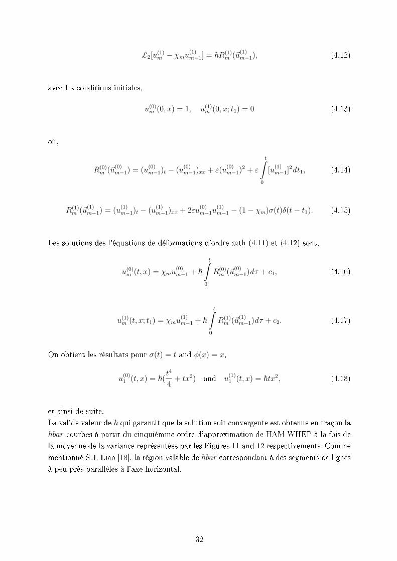
Les solutions des l'équations de déformations d'ordre mth (4.11) et (4.12) sont,
u(0)m (t, x) = χmu
(0)m−1 + ~
t∫0
R(0)m (u
(0)m−1)dτ + c1, (4.16)
u(1)m (t, x; t1) = χmu
(1)m−1 + ~
t∫0
R(1)m (u
(1)m−1)dτ + c2. (4.17)
On obtient les résultats pour σ(t) = t and ϕ(x) = x,
u(0)1 (t, x) = ~(
t4
4+ tx2) and u
(1)1 (t, x) = ~tx2, (4.18)
et ainsi de suite.
La valide valeur de ~ qui garantit que la solution soit convergente est obtenue en traçon la
hbar-courbes à partir du cinquièmme ordre d'approximation de HAM WHEP à la fois de
la moyenne de la variance représentées par les Figures 11 and 12 respectivements. Comme
mentionné S.J. Liao [18], la région valable de hbar correspondant à des segments de lignes
à peu près parallèles à l'axe horizontal.
32

-2.0 -1.5 -1.0 -0.5h
0.44
0.46
0.48
0.50
Μu H0.1LÆHxL=x=0.5,Ε=1
Fig. 11: La ~-courbe de l'espérance obtenue par la cinquième ordre d'approximation HAM
WHEP
-2.0 -1.5 -1.0 -0.5h
0.000315
0.000320
0.000325
0.000330
Σu2 H0.1L
ÆHxL=x=0.5,Ε=1
Fig. 12: La ~-courbe de la variance obtenue par la cinquième ordre d'approximation HAMWHEP
Maintenant, compte tenu du cas n = 3, l'équation (0.2) d'intérêt dans le présent
document devient,
∂u(t, x;ω)
∂t=
∂2u(t, x;ω)
∂x2− εu3(t, x;ω) + σ(t).n(t, ω); (t, x) ∈ (0,∞)× (0, L),
u(t, 0) = u(t, L) = 0, u(0, x) = ϕ(x), (4.19)
où σ(t).n(t, ω) est le processus en temps de bruit blanc produit par σ(t) : σ(t) est la partie
de temps continu de la force aléatoire.
En procédant de la même manière que précédemment. La valide valeur de ~ qui garantit
que la solution soit convergente est obtenue en traçon la hbar-courbes à partir du qua-
trièmme ordre d'approximation de HAM WHEP à la fois de la moyenne de la variance
représentées par les Figures 13 and 14 respectivements. Comme mentionné S.J. Liao [18],
33

la région valable de hbar correspondant à des segments de lignes à peu près parallèles à
l'axe horizontal.
-2.5 -2.0 -1.5 -1.0 -0.5h
0.55
0.60
Μu H0.1Lx=0.5,Ε=1
Fig. 13: La ~-courbe de l'espérance obtenue par la quatrième ordre d'approximation HAM
WHEP
-2.0 -1.5 -1.0 -0.5 0.5 1.0h
0.00040
0.00045
0.00050
0.00055
Σu2 H0.1L
ΦHxL=0.5,Ε=1
Fig. 14: La ~-courbe de la variance obtenue par la quatrième ordre d'approximation HAMWHEP
34

Conclusion
Cette thèse est cosacrée à l'étude d'une nouvelle approche qu'on appelle la méthode
Homotopie et l'Analyse liée au développement de Wiener Hermite et la Perturbation
et l'appliquée pour résoudre une certaine classe d'équations diérentielles stochastiques.
L'avantage de ctte méthode est de surmanter les diucltées résultantes de la méthode de
la Homotopie et la perturbation car l'utlisation des méthodes perbatives peut conduire
à divergence de solution et le choix doit etre bon de de la condition initiale dans la
méthode de Homotpie et de perturbetion pour qu'on puisse garantir la convergence de
la solution. La méthode Homotopie et d'Analyse utilise un paramètre ~ de controle la
région de convergence de la série de la solution et on a une grande liberté de choisir la
condition initiale ce qui est diérent de HPM. La méthode a été applliquée avec succée
sur une certaine classe d'EDS dont nous avons eu la convergence de la série de la solution
les résultats sont interprétés par des courbes . Touts les résultas prouvent l'imporatance
de la nouvelle approche.
Actuellement nous nous somme interrsser par l'application de la nouvelle approche pour
résoudre l'équation de Navier Stokes à une dimenssion .
35

Bibliographie
[1] S. Abbasbandy, E. Magyari, E. Shivanian, The homotopy analysis method for
multiple solutions of nonlinear boundary value problems, Communications in Nonlinear
Science and Numerical Simulation, 14 (9-10) (2009), 3530 - 3536
[2] S. Abbasbandy, Approximate solution for the nonlinear model of diusion and
reaction in porous catalysts by means of the homotopy analysis method, Chemical
Engineering Journal, 136 (2-3)(2008), 144-150.
[3] M.A. El-Tawil, The Homotopy Wiener Hermite Expansion and Perturbation
technique (WHEP), Transactions on Computational Science I, 4750(2008), 159-180.
[4] M.A. El-Tawil, The application of WHEP technique on partial dierential equations,
International Journal of Dierential Equations and Applications,7 (3)(2003), 325-337.
[5] M.A. El-Tawil, Nonhomogeneous boundary value problems, Journal of Mathematical
Analysis and Applications,200(1996), 53-65.
[6] M.A. El-Tawil, N. A. Al-Mulla, Using Homotopy WHEP technique for solving a
stochastic nonlinear diusion equation, Mathematical and Computer
Modelling,51(2010), 1277-1284.
[7] A. Boukehila, F. Z. Benmostefa, Solution process of a class of dierential equation
using homotopy analysis Wiener Hermite expansion and perturbation
technique,8(2014),n.4,167-186.
[8] M.A. El-Tawil, A. Fareed, Solution of Stochastic Cubic and Quintic Nonlinear
Diusion Equation Using WHEP, Pickard and HPM Methods, Open Journal of Discrete
36

Mathematics,1(1) (2011), 6-21.
[9]M.A. El-Tawil, G. Mahmoud, The solvability of parametrically forced oscillators using
WHEP technique, Mechanics and Mechanical Engineering,3 (2)(1999), 181-188.
[10] M.A. El-Tawil, The average solution of a stochastic nonlinear Schrodinger equation
under stochastic complex non-homogeneity and complex initial conditions, Transactions
on Computational Science III,5300 (2009), 143-170.
[11] C. Eftimiu, First-order Wiener Hermite Expansion in the electromagnetic scattering
by conducting rough surfaces, Radio Science,23 (5)(1980), 769-779.
[12] J.H. He, Comparison of homotopy perturbation method and homotopy analysis
method, Applied Mathematics and Computation,156 (2)(2004), 527-539.
[13] I. Hashim, O. Abdulaziz, S. Momani, Homotopy analysis method for fractional
IVPs, Communications in Nonlinear Science and Numerical Simulation,14 (3) (2009),
674-684.
[14] T. Imamura, W. Meecham, A. Siegel, Symbolic calculus of the Wiener process and
Wiener Hermite Functionals, Journal of Mathematical Physics,6 (5)(1983), 695-706.
[15]H. Jafari, S. Sei, Homotopy analysis method for solving linear and nonlinear
fractional diusion wave equation, Communications in Nonlinear Science and Numerical
Simulation,14 (2009), 2006-2012.
[16] P. E. Kloeden, and E. Platen, Numerical Solution of Stochastic Dierential
Equations,Springer, Berlin, 1995.
[17] S.J, Liao, The proposed homotopy analysis technique for the solution of nonlinear
problems,PhD, Dissertation, Shanghai, Shanghai Jiao Tong University, 1992.
[18] S.J. Liao, Beyond Perturbation Introduction to the Homotopy Analysis Method,CRC
37

Press, Boca Raton, Chapman and Hall, Boca Raton, 2003.
[19] S.J. Liao, Comparison between the homotopy analysis method and homotopy
perturbation method, Applied Mathematics and Computation,169(2005), 1186-1194.
[20] S.J. Liao, A new branch of solutions of boundary layer ows over an impermeable
stretched plate, International Journal of Heat and Mass Transfer,48(2005), 2529-39.
[21] I. Orabi, I. Ahmadi, A. Goodarz, A Functional Series Expansion Method for
Response Analysis of Nonlinear Systems Subjected to Random Excitations,
International Journal of NonLinear Mechanics,22 (6) (1987), 451-465
[22] B. Oksendal, Stochastic Dierential Equations : An Introduction with Application,
Springer, Berlin, 1998.
[23] P. Saman, Application of Wiener Hermite Expansion to the diusion of a passive
scalar in a homogeneous turbulent ow, Physics of Fluids,12 (9) (1969), 1786-1798.
[24] B. Oksendal, Stochastic Dierential Equations : An introduction with application,
Third Edition, Springer, 1989.
[25] B. Zdzislaw,T. Zastawniak Basic Stochastic Process, A course Through Exercices,
Springer, 1998.
[26] Kampe de Feriet, Random solutions of partial dierential equations, in : Proc. 3rd
Berkeley Symposium on Mathematical Statistics and Probability- 1955, vol. III, 1956,
pp. 199-208.
[27] R. Bharucha, A survey on the theory of random functions, The Institute of
Mathematical Sciences : Mat science Report 31, India, 1965.
[28] V. Lo Dato, Stochastic processes in heat and mass transport, C, in : Bharucha-Reid
38

(Ed.), Probabilistic Methods in Applied Mathematics, vol. 3, A.P., 1973, pp. 183-212.
[29] A. Georges Becus, Random generalized solutions to the heat equations, J. Math.
Anal. Appl. 60 (1977) 93-102.
39

Appendice
Les Polynômes de Wiener-Hermite
La méthode de développement de Wiener Hermite WHE utilise Les Polynômes de
Wiener-Hermite dont ils sont des éléments d'un ensemble complet des variables aléa-
toires statistiquement ortogonales. Chaque fonction aléatoire G(t), peut etre développée
en terme des Polynômes de Wiener-Hermite H(n)(t1, t2, . . . , tn) as :
G(t) =∞∑n=0
ξ(n)G(n)(t1, t2, . . . , tn)H(n)(t1, t2, . . . , tn)dt
(n) (B.1)
ξ(n) =
∫ ∞
−∞
∫ ∞
−∞. . .
∫ ∞
−∞
dt(n) = dt1dt2 . . . dtn (B.2)
où G(n)(t1, t2, . . . , tn) sont les noyaux en fonction de temps t.
Les Polynômes de Wiener-Hermite H(n)(t1, t2, . . . , tn) satisfait la relation de récurrence
suivante :
H(n)(t1, t2, . . . , tn) = H(n−1)(t1, t2, . . . , tn−1)H(n)(tn)
−n−1∑i=1
H(n−2)(t1, . . . , tn−2).δ(tn−m − tn), i ≥ 2, n ≥ 2 (B.3)
For example
H(0) = 1
H(1)(t) = n(t)
H(2)(t1, t2) = H(1)(t1)H(1)(t2)− δ(t1 − t2)
H(3)(t1, t2, t3) = H(2)(t1, t2)H(1)(t3)−H(1)(t1)δ(t2 − t3)−H(1)(t2)δ(t1 − t3) (B.4)
où n(t) est processus de Bruit blanc, en particulier on a :
En(t) = 0, En(t1)n(t2) = δ(t1 − t2) (B.5)
40

où δ(−) est la fonction de Dirac, tel que pour toutes fonction f(x) on :,∫f(x)δ(y − x)dx = f(y) (B.6)
L'ensemble de Wiener-Hermite est statistiquement orthogonale, i.e.
EH(i).H(j) = 0 ∀i = j (B.7)
Propriétés des Polynômes de Wiener-Hermite
H i and Hj sont orthogonales, i.e ;
EH(i)(t1, t2, . . . , ti)H(j)(t1, t2, . . . , tj) = 0, ∀i = j (B.8)
La moyenne pour touts les H s'annule, en particulier,
EH(i)(t1, t2, . . . , ti) = 0, i ≥ 1 (B.9)
EH(2)(t1, t2)H(2)(t3, t4) = δ(t1 − t3)δ(t2 − t4) + δ(t1 − t4)δ(t2 − t3) (B.10)
EH(1)(t1)H2(t2, t3)H
(1)(t4) = δ(t1 − t2)δ(t3 − t4) + δ(t1 − t3)δ(t2 − t4) (B.11)
EH(2)(t1, t2)H1(t3)H
(1)(t4) = δ(t1 − t4)δ(t2 − t3) + δ(t2 − t4)δ(t1 − t3) (B.12)
EH(1)(t1)H1(t2)H
2(t(3), t4) = δ(t1 − t3)δ(t2 − t4) + δ(t1 − t4)δ(t2 − t3) (B.13)
EH(1)(t1)H(1)(t2) . . . H
(1)(ti) = 0, odd (B.14)
EH(1)(t1)H(1)(t2)H
(1)(t3) = 0 (B.15)
EH(1)(t1)H(1)(t2)H
(1)(t3)H(1)(t4) = δ(t1 − t2)δ(t3 − t4) + δ(t1 − t3)δ(t2 − t4)
+ δ(t1 − t4)δ(t2 − t3) (B.16)
EH(l)H(m) = 0, l +m = odd (B.17)
E(
∫ t
0
σ(τ)n(τ)dτ) =
∫ t
0
σ(τ)En(τ)dτ = 0 (B.18)
E(
∫ t
0
σ(τ)n(τ)dτ)2 = E(
∫ t
0
σ(τ1)n(τ1)dτ1)(
∫ t
0
σ(τ2)n(τ2)dτ2)
=
∫ t
0
∫ t
0
σ(τ1)σ(τ2)En(τ1)n(τ2)dτ1dτ2
=
∫ t
0
∫ t
0
σ(τ1)σ(τ2)δ(τ1 − τ2)dτ1dτ2
=
∫ t
0
(σ(τ1))2dτ1,whenτ2 → τ1 (B.19)
41

Les Polynômes de Wiener-Hermite sont symétriques ;
H(i)(t1, t2, . . . , tl, . . . , tm, . . . , ti) = H(i)(t1, t2, . . . , tm, . . . , tl, . . . , ti) (B.20)
42

Int. Journal of Math. Analysis, Vol. 8, 2014, no. 4, 167 - 186 HIKARI Ltd, www.m-hikari.com
http://dx.doi.org/10.12988/ijma.2014.312303
Solution Process of a Class of Differential Equation Using Homotopy Analysis Wiener Hermite
Expansion and Perturbation Technique
A. Boukehila
Department of Mathematics, Faculty of Sciences, Badji Mokhtar University. PO Box 12, 23000 Annaba, Algeria
F. Z. Benmostefa
Numerical Analysis, Optimization and Statistical Laboratory Department of Mathematics, Faculty of Sciences, Badji Mokhtar
University. PO Box 12, 23000 Annaba, Algeria
Copyright © 2014 A. Boukehila and F. Z. Benmostefa. This is an open access article distributed under the Creative Commons Attribution License, which permits unrestricted use, distribution, and reproduction in any medium, provided the original work is properly cited.
Abstract
In this paper, we construct a new method based on the Homotopy analysis method (HAM) linked to Wiener Hermite expansion perturbation (WHEP) technique and it is called HAM WHEP and then apply it to solve the generalized stochastic nonlinear diffusion equation with square or cubic nonlinear losses by obtaining the average and variance of the solution process. The aim of applying this new technique is to overcome the difficulties arising from the Homotopy perturbation method (HPM). Accordingly, applying HPM linked to WHEP in [6] may lead to divergence. This disadvantage is overcome by using the HAM which guarantees the convergence of the series solution. In this direction, this paper revisits and solves the sto-

168 A. Boukehila and F. Z. Benmostefa chastic nonlinear diffusion equation in [6] by applying the HAM WHEP technique. All test problems reveal the accuracy and the convergence of the suggested method.
Mathematics Subject Classification: 65L05; 34A25; 34B15 Keywords: Stochastic nonlinear diffusion equation; Homotopy analysis method; Wiener hermite expansion; Homotopy analysis wiener hermite expansion and perturbation technique
1 Introduction The mathematical modeling of many real-life phenomena by reason of random perturbation are not possible by ordinary differential equations, and hence are often modeled by using stochastic differential equations in order for the model to become more realistic [16, 22]. Because such differential equations cannot usually be solved analytically, the study of numerical methods is required and these must be designed to perform with a certain order of accuracy. Many authors investigated the stochastic diffusion equation under different views [5, 21]. Recently, M.A. El-Tawil used the Wiener Hermite expansion together with Perturbation theory (WHEP) technique to solve a perturbed nonlinear stochastic diffusion equation [4]. The technique has been then developed to be applied on non-perturbed differential equations using the Homotopy perturbation Method linked to Wiener Hermite expansion perturbation technique and it is called Homotopy WHEP [3]. However, as mentioned S.J. Liao [19], Homotopy perturbation method (HPM) is only a special case of the Homotopy analysis method (HAM). The difference is that, the HPM had to use a good enough initial guess, but this is not absolutely necessary for the HAM. This is mainly because the HAM uses a so-called convergence control parameter to guarantee the convergence of approximation series over a given interval of physical parameters. So, the Homotopy analysis method (HAM) is more general. In 2010, M.A. El-Tawil and N.A. Al-Mulla [6] used the HPM linked to WHEP technique to solve the stochastic nonlinear diffusion equation with square or cubic nonlinear losses, as follows,
( ) ( ) ( ) ( );;.;,;,;,2
2
ωσωεωω tnxtux
xtutxtu n +−
∂∂
=∂
∂ ( ) ( ) ( ),,0,0; Lxt ×∞∈ (1)
( ) ( ) ( ) ( )xxuLtutu φ=== ,0,0,0, , where the viscosityε is a deterministic scale for the nonlinear term. The non homogeneity term ( )tn.σ is a time white noise process scaled by σ . However, solving the stochastic nonlinear diffusion equation (1) mentioned

Solution process of a class of differential equation 169 above did not consider the influence of using the HPM on the convergence of the series solution. In fact, there is absolutely no guarantee that perturbation methods result in a convergent solution. Accordingly, using the HPM linked to WHEP in [6] may lead to divergence. This disadvantage is overcome by using the Homotopy analysis method (HAM) linked to WHEP (HAM WHEP) technique. In this direction, this paper revisits and solves the stochastic nonlinear diffusion equation in [6] by applying the HAM WHEP technique. All test problems reveal the accuracy and convergence of the suggested new method. The main aim of this paper is to construct and develop a new approach based on the Homotopy analysis method introduced in WHEP (HAM WHEP) technique and then apply it for solving the diffusion equation under square and cubic nonlinearities and stochastic non-homogenous on a class of differential equations. Some statistical moments are obtained, mainly the ensemble average and variance of the solution process with corresponding figures. In this study, for our aim we consider the generalized stochastic nonlinear diffusion equation with square or cubic losses 2uε or 3uε of interest is of the following form,
( ) ( ) ( ) ( ) ( );;.;,;,;,2
2
ωσωεωω tntxtux
xtutxtu n +−
∂∂
=∂
∂ ( ) ( ) ( ),,0,0; Lxt ×∞∈ (2)
( ) ( ) ( ) ( )xxuLtutu φ=== ,0,0,0, , where is a deterministic scale for the nonlinear term and 3,2=n . ( )P,,σω Ω∈ is a triple probability space with as the sample space, σ is a σ -algebra on events in Ω and P is a probability measure. The physical meaning of the nonlinear term is that there exists a loss proportional to 2u or to 3u . The non homogeneity term ( ) ( )ωσ ,. tnt is a time white noise process scaled by ( )tσ : ( )ωσ ;t is a continuous time part of the random forcing.
2 The Wiener Hermite Expansion and Perturbation Technique The application of the Wiener Hermite expansion and perturbation (WHEP) technique [7, 8, 9, 10, 11, 14, 23] aims at finding a truncated series solution to the stochastic solution process of stochastic differential equations. The truncated series is composed of two major parts; the first is the Gaussian part which consists of the first two terms, while the rest of the series constitute the non-Gaussian part. In nonlinear cases, there exist always difficulties of solving the resultant set of deterministic integro-differential equations got from the applications of a set of comprehensive averages on the stochastic integro-differential equation obtained after the direct application of WHE. Due to the completeness of the wiener Hermite set, any random function ( )ω;tG

170 A. Boukehila and F. Z. Benmostefa can be expanded as follows, ( ) ( ) ( ) ( ) ( ) ( ) ( ) ( ) ( ) ( ) ( ) ..,,;; 2121
221
211
11
10 +++= ∫ ∫ ∫ℜ ℜℜ
dtdtttHtttGdttHttGtGtG (3)
Where the first two terms are the Gaussian part of ( )ω;tG . The rest of the terms in the expansion represent the non-Gaussian part of ( )ω;tG . The average of ( )ω;tG is
( ) ( ) ( )tGtEGG0; == ωμ with ( ) ( ) ( ) ( ) ( ) ( ) ( ),.,0 212
11
11
1 tttHtEHtEH −== δ (4)
where the time white noise process is ( ) ( ) ( )11
1 tHtn = . The covariance of ( )ω;tG is
( ) ( )( ) ( ) ( )( ) ( ) ( )( )τμωτμωωτω GG GttGEGtGCov −−= ;;;,;
( ) ( ) ( ) ( ) ( ) ( ) ( ) ( ) ...,;,;2;; 21212
212
111
11 ++= ∫ ∫ ∫
ℜ ℜℜ
dtdtttGtttGdttGttG ττ (5)
The variance of ( )ω;tG is
( ) ( )( )22 ; ttGE GG μωσ −=
( ) ( )[ ] ( ) ( )[ ]∫ ∫ ∫ℜ ℜℜ
++= ...,;2; 212
212
12
11 dtdttttGdtttG (6)
The WHEP technique can be applied on linear or nonlinear perturbed systems described by ordinary or partial differential equations. The solution can be modified in the sense that additional parts of the Wiener Hermite expansion can be taken into considerations and the required order of approximations can always be made depending on the computing tool. The first order solution can be obtained when considering only the Gaussian part of the solution process ( )ω;tu can be expanded as, ( ) ( ) ( ) ( ) ( ) ( ) ( ) 11
11
10 ;; dttHttututu ∫ℜ
+=ω . (7)
The WHEP technique uses the following expansion for its deterministic kernels, ( ) ( ) ( ) ( ) ( ) ,...1,0...,2
210 =+++= iuuutu iiii εε (8)
3 Basic idea of Homotopy Analysis Method The Homotopy analysis method (HAM) initially proposed by S.J. Liao in his

Solution process of a class of differential equation 171 Ph.D. thesis [17]. A systematic and clear is exposition on the HAM is given in [18]. In recent years, this method has been successfully employed to solve many types of nonlinear problems in science and engineering [1, 2, 13, 15, 20]. HAM contains a certain auxiliary parameterh , which provides with a simple way to adjust and control the convergence region and rate of convergence of the series solution. Moreover, by means of the so-called h -curve, a valid region of h can be studied to gain a convergent series solution. It is important to note that, one has great freedom to choose auxiliary objects such as h and L in HAM. Thus, through HAM, explicit analytic solutions of nonlinear problems are possible. To describe the basic idea of the HAM, we consider the following differential equation, ( )[ ] ,0, =Ν txu (9) where Ν is a nonlinear operator, x and t denotes the independent variables, ( )txu , is an unknown function, respectively. By means of generalizing the
traditional Homotopy method, S.J. Liao [17] construct the so-called zero order deformation equation, ( ) ( ) ( )[ ] ( ) ( )[ ],;,,,;,£1 0 qtxNtxHqtxuqtxq ψψ h=−− (10) where [ ]1,0∈q is an embedding parameter, h is the nonzero auxiliary parameter and ( )txH , is the nonzero auxiliary function, £ is an auxiliary linear operator,
( )txu ,0 is an initial guess of ( )txu , and ( )qtx ;,ψ is an unknown function. Obviously, when 0=q and 1=q both, ( ) ( )txutx ,0;, 0=ψ and ( ) ( ),,1;, txutx =ψ (11) respectively hold. Thus as q increases from 0 to 1, the solution ( )qtx ;,ψ varies from the initial guess ( )txu ,0 to the solution ( )txu , . Expanding ( )qtx ;,ψ in Taylor series with respect to q , one has, ( ) ( ) ( ) ,,,;,
10m
m m qtxutxuqtx ∑∞
=+=ψ (12)
where,
( ) ( ) .;,!
1,0=∂
∂=
qm
m
m qqtx
mtxu ψ (13)
If the auxiliary linear operator, the initial guess, the auxiliary parameter h and the auxiliary function are so properly chosen, then the series (12) converges at
1=q and,

172 A. Boukehila and F. Z. Benmostefa ( ) ( ) ( ),,,,
10 txutxutxum m∑∞
=+= (14)
which is the solution of the original equation, as proved by S.J. Liao [30]. As ( ) 1, =txH and ,1−=h Equation (10) becomes,
( ) ( ) ( )[ ] ( )[ ] ,0;,,;,£1 0 =+−− qtxqNtxuqtxq ψψ (15) which is used mostly in the Homotopy perturbation method (HPM) proving that the HPM is a special case of the Homotopy analysis method (HAM). Comparison between the HAM and HPM can be found in [12, 19]. According to equation (13), the governing equation can be deduced from the zero order deformation equation (10). Define the vector, ( ) ( ) ( ) .,,...,,,, 10 txutxutxuu nn = (16) Differentiating (10) m times with respect to the embedding parameter q and then setting 0=q and finally dividing them by !m , we have the so-called mth order deformation equations, ( ) ( )[ ] ( ) ( )11 ,,,£ −− =− mmmmm uRtxHtxutxu hχ , (17) where
⎩⎨⎧
>≤
=1,11,0
mm
mχ (18)
and
( ) ( )( )[ ]
01
1
1;,
!11
=−
−
−∂
∂−
=q
m
m
mm qqtxN
muR ψ . (19)
For any given nonlinear operator N and the term ( )1−mm uR can be easily expressed by equation (19). So we can obtain ( ) ( ),...,,, 21 txutxu by means of solving the linear high order deformation equation (17). The mth order approximation of ( )txu , is given by,
( ) ( )∑∞
==
0,,,
m m txutxu (20) The foregoing approximate solution consist of which is a cornerstone of the HAM in determining convergence of series solution rapidly. We may adjust

Solution process of a class of differential equation 173 and control the convergence region and rate of the solution series (20) by means of the auxiliary parameter . To obtain valid region of , we first plot the so called -curves of ( )txu , , ( )
α=xt txu , where [ ]ba,∈α and so on. According to these h -curves, it is easy to discover the valid region of h , which corresponds to the line segments nearly parallel to the horizontal axis. Theorem 3.1 According to S.J. Liao [18], as long as the series (20) converges to ( )txu , , where ( )txum , is governed by the high-order deformation equation (17) under the definitions (18) and (19), it is must be the exact solution of equation (9). 4 Solving the Langevin equation using some techniques: HAM, WHEP and HAM WHEP technique
This section deals with the Langevin equation by using three techniques, in particular: WHEP, HAM and HAM WHEP technique. We consider the Langevin equation for 3,2=n ,
( ) ( ) ( ) ( ) ( )
( ) ,10
,,0,;.;;
=
∞∈+−=∂
∂
u
ttnttut
tu n ωσωεω (21)
where ( )ω;tn is the time white noise process, ( )tσ is a continuous function and ε is a constant. 4.1 Using WHEP technique for solving the Langevin equation At 2=n , Eq.(21) recasts as,
( ) ( ) ( ) ( ) ( )
( ) ,10
,,0,;.;; 2
=
∞∈+−=∂
∂
u
ttnttut
tu ωσωεω (22)
where ( ).tσ is the time white noise process scled by : is a continuous function and is a constant. Applying the WHEP technique on Eq. (22) and taking the necessary averages, we get the following equations,
( ) ( ) ( ) ( )[ ] ( ) ( )[ ] 1
2
0 1120
0
; dtttutut
tu t
∫−−=∂
∂ εε , (23)

174 A. Boukehila and F. Z. Benmostefa
( ) ( ) ( ) ( ) ( ) ( ) ( ) ( ).;2;
11101
1
tttttutut
ttu−+−=
∂∂
δσε (24)
Where,
( ) ( ) ( ) ( ) ( ) ( ) ( ) .;; 111
0
10 dttHttututut
∫+=ω (25)
Applying the perturbation technique, the deterministic kernels can be represented in first order approximation as, ( ) ( ) ( ) ( ) ( ) ( )tututu 0
10
00 ε+= , (26)
( ) ( ) ( ) ( ) ( ) ( )1
111
101
1 ;;; ttuttuttu ε+= . (27) The solution is to evaluate ( )0
0u and ( )10u and then computing the other two
kernels independently. The final results of the first order first correction mean and variance respectively are, ( ) ( ) ( )tutu
0=μ , (28)
( ) ( ) ( )[ ] .; 10
21
12 dtttutt
u ∫=σ (29)
4.2 Using HAM for solving the Langevin equation In order to solve Eq. (22) by the HAM, we choose the initial approximation, ( ) ,10 =tu (30) and the auxiliary linear operator,
( )[ ] ( ) ,;;£t
qtqt∂
∂=
ψψ (31)
with the property, [ ] ,0£ 1 =c (32) where 1c is an integral constant. Furthermore, Eq. (22) suggests that we define the nonlinear,

Solution process of a class of differential equation 175
( )[ ] ( ) ( ).; 2 tntt
qtN σεψψψ −+∂∂
= . (33)
Using the above definition, we construct the zero order deformation equation ( ) ( ) ( )[ ] ( ) ( )[ ]qtNtHqtuqtq ;;£1 0 ψψ h=−− . (34) As ( ) 1=tH , Eq. (34) becomes, ( ) ( ) ( )[ ] ( )[ ]qtNqtuqtq ;;£1 0 ψψ h=−− , (35) and the so-called mth order deformation equation,
( ) ( )[ ] ( )11£ −− =− mmmmm uRtutu hχ , (36) with the initial condition, ( ) 00 =mu , (37) where ( ) ( ) ( ) ( ) ( ) ( )tntuuuR mmtmmm σχε −−+= −−− 12
111 . (38) Now, the solution of the so-called mth order deformation equation Eq. (36) for
1≥m becomes,
( ) ( ) ( ) 1011 cduRtutu
tmmmmm ++= ∫ −− τχ h , (39)
where the integration constant 1c is determined by the initial condition (37). Taking the necessary averages with ( ) tt =σ , we get the following results when getting both the fourth order approximation for the mean and the variance respectively,
( )( ) [ ] ( ) ( )
( ) ,8132149
1013
1233321
96
86
76
623
54
422
3234
2
tttt
tttttu
hhhhhh
hhhhhhhhhhh
++++
−
++
++
+++++++=μ
(40)

176 A. Boukehila and F. Z. Benmostefa
( ) ( ) ( ) 86
76
54
322
2
93312
3tttttu
hhhhhh++
++
+=σ . (41)
The proper value of h which ensures that the approximation solution is convergent is found from the h -curves obtained both from the fourth order HAM approximation of the mean and the variance shown in Figures 1 and 2 respectively. The valid region of h corresponds to the line segments nearly parallel to the horizontal axis.
Figure 1: The h -curve of the mean based on the fourth order HAM approximation
Figure 2: The -curve of the variance based on the fourth order HAM approximation

Solution process of a class of differential equation 177
4.3 Using HAM WHEP technique for solving the Langevin equation Applying the WHEP technique on the proposed example of the Eq. (22), and taking the necessary averages, we get the following equations,
( ) ( ) ( ) ( )[ ] ( ) ( )[ ] 1
2
0 1120
0
; dtttutut
tu t
∫−−=∂
∂ εε (42)
( ) ( ) ( ) ( ) ( ) ( ) ( ) ( )11
1011
;2; tttttutut
ttu−+−=
∂∂
δσε . (43)
In order to solve the Eqs. (42) and (43) by the HAM, we choose the initial approximations
( ) ( ) ( ) ( ) tttutu == 10
00
0 ;,1 . (44) Applying the same approach as in subsection (4.2) with ( ) tt =σ . The proper value of h is found from the h -curves obtained from the sixth order HAM WHEP approximation of the mean and the fifth order HAM WHEP approximation of the variance shown in Figures 3 and 4 respectively. The valid region of h corresponds to the line segments nearly parallel to the horizontal axis.
Figure 3: The h -curve of the mean obtained from the sixth order HAM WHEP approximation

178 A. Boukehila and F. Z. Benmostefa
Figure 4: The h -curve of the variance obtained from the fifth order HAM WHEP approximation
Now, considering the case 3=n , and proceeding in a similar manner as in subsection 4.3, the results are obtained from the h -curves both of the fourth order HAM WHEP approximation of the mean and the variance shown in Figures 5 and 6 respectively. The valid region of h corresponds to the line segments nearly parallel to the horizontal axis.
Figure 5: The h -curve of the mean obtained from the fourth order HAM WHEP approximation

Solution process of a class of differential equation 179
Figure 6: The h -curve of the variance obtained from the fourth order HAM WHEP approximation
Concerning only a first order approximation, it can be noticed both the HAM and HAM WHEP techniques give near results. The HAM WHEP technique seems an efficient one because of its correction possibilities. 5. Solving the Boundary value problem using Homotopy Analysis Wiener Hermite Expansion and Perturbation technique In the present paper, for our aim, the HAM WHEP technique is applied to solve the generalized stochastic nonlinear diffusion equation with square or cubic losses, 2uε or 3uε and it is shown that how one can control the convergence of approximate solution and make the convergence fast. At 2=n , the equation (2) of interest in this paper becomes,
( ) ( ) ( ) ( ) ( );;.;,;,;, 22
2
ωσωεωω tntxtux
xtutxtu
+−∂
∂=
∂∂ ( ) ( ) ( ),,0,0; Lxt ×∞∈ (45)
( ) ( ) ( ) ( )xxuLtutu ϕ=== ,0,0,0, , where ( ).tσ ( )ω;tn is the time white noise process scaled by ( )tσ : ( )tσ is the continuous time part of the random forcing. Applying the WHEP technique on the proposed equation in (45), and taking the necessary averages, we get the following equations,
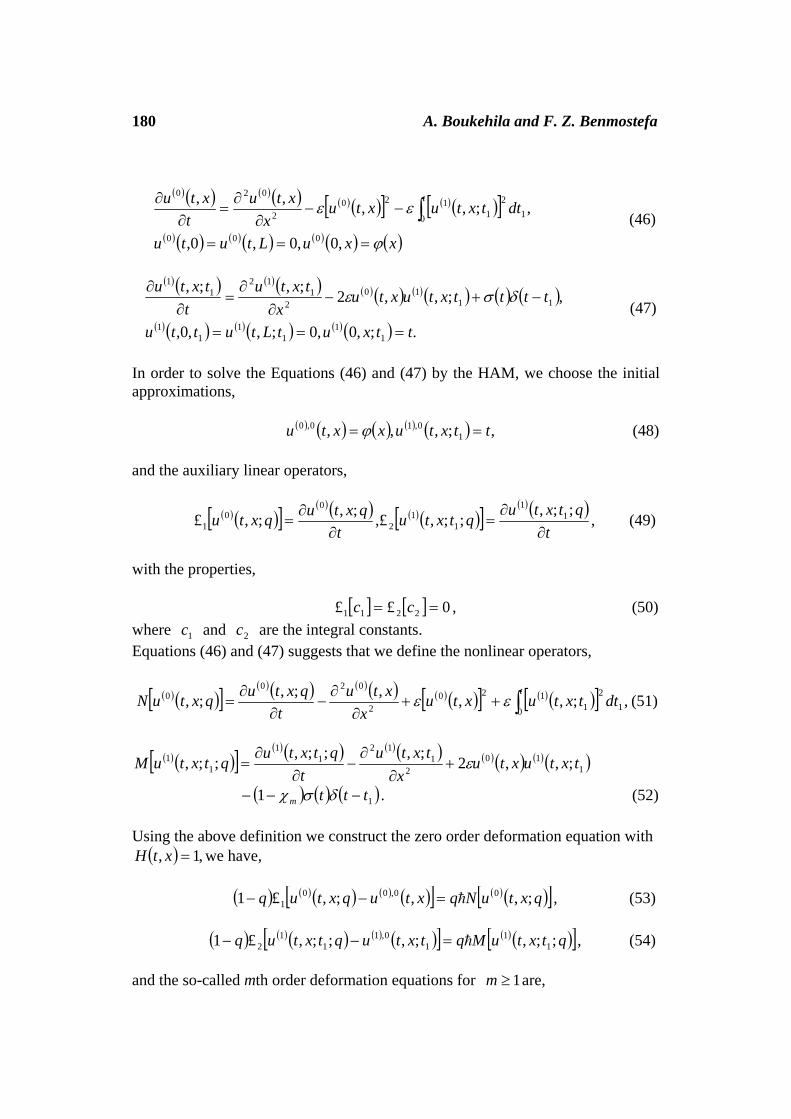
180 A. Boukehila and F. Z. Benmostefa
( ) ( ) ( ) ( ) ( ) ( )[ ] ( ) ( )[ ]( ) ( ) ( ) ( ) ( ) ( ) ( )xxuLtutu
dttxtuxtux
xtut
xtu t
ϕ
εε
===
−−∂
∂=
∂∂
∫,0,0,0,
,;,,,,
000
0 12
1120
2
020
(46)
( ) ( ) ( ) ( ) ( ) ( ) ( ) ( ) ( ) ( )( ) ( ) ( ) ( ) ( ) ( ) .;,0,0;,,0,
,;,,2;,;,
11
11
11
1110
21
121
1
ttxutLtuttu
ttttxtuxtux
txtut
txtu
===
−+−∂
∂=
∂∂
δσε (47)
In order to solve the Equations (46) and (47) by the HAM, we choose the initial approximations, ( ) ( ) ( ) ( ) ( ) ,;,,, 1
0,10,0 ttxtuxxtu == ϕ (48) and the auxiliary linear operators,
( ) ( )[ ]( ) ( ) ( ) ( )[ ]
( ) ( ),;;,;;,,£;,;,£ 1
1
11
2
00
1 tqtxtuqtxtu
tqxtuqxtu
∂∂
=∂
∂= (49)
with the properties, [ ] [ ] 0££ 2211 == cc , (50) where 1c and 2c are the integral constants. Equations (46) and (47) suggests that we define the nonlinear operators,
( ) ( )[ ]( ) ( ) ( ) ( ) ( ) ( )[ ] ( ) ( )[ ] ,;,,,;,;,
0 12
1120
2
0200 ∫++
∂∂
−∂
∂=
tdttxtuxtu
xxtu
tqxtuqxtuN εε (51)
( ) ( )[ ]
( ) ( ) ( ) ( ) ( ) ( ) ( ) ( )110
21
121
1
11 ;,,2;,;;,;;, txtuxtu
xtxtu
tqtxtuqtxtuM ε+
∂∂
−∂
∂=
( ) ( ) ( )11 tttm −−− δσχ . (52) Using the above definition we construct the zero order deformation equation with ( ) ,1, =xtH we have,
( ) ( ) ( ) ( ) ( )[ ] ( ) ( )[ ]qxtuNqxtuqxtuq ;,,;,£1 00,00
1 h=−− , (53) ( ) ( ) ( ) ( ) ( )[ ] ( ) ( )[ ]qtxtuMqtxtuqtxtuq ;;,;,;;,£1 1
11
0,11
12 h=−− , (54)
and the so-called mth order deformation equations for 1≥m are,

Solution process of a class of differential equation 181
( ) ( )[ ] ( ) ( ),£
1,0,01,0,01 ⎟
⎠⎞⎜
⎝⎛=−
−− mmmm
m uRuu hχ (55)
( ) ( )[ ] ( ) ( )⎟⎠⎞⎜
⎝⎛=−
−− 1,1,11,1,12£
mmmm
m uRuu hχ , (56)
with the initial conditions, ( ) ( ) ( ) ( ) 0;,0,1,0 1
,1,0 == txuxu mm , (57) where,
( ) ( ) ( )( ) ( )( ) ( )( ) ( )[ ] ,1
2
0
1,121,01,01,01,0,0 dtuuuuuRt mm
xxm
tmmm ∫ −−−−−
++−=⎟⎠⎞⎜
⎝⎛ εε (58)
( ) ( ) ( )( ) ( )( ) ( ) ( ) ( ) ( ) ( )1
1,11,01,11,11,1,1 12 tttuuuuuR mmm
xxm
tmmm −−−+−=⎟
⎠⎞⎜
⎝⎛ −−−−−
δσχε . (59)
The solutions of the so-called mth order deformation equation (55) and (56) are,
( ) ( ) ( ) ( ) ( ),, 10
1,0,01,0,0 cduRuxtut mmm
mm +⎟
⎠⎞⎜
⎝⎛+= ∫
−− τχ h (60)
( ) ( ) ( ) ( ) ( )20
1,1,11,1,1 , cduRuxtut mmm
mm +⎟
⎠⎞⎜
⎝⎛+= ∫
−− τχ h . (61)
We obtain the results for ( ) tt =σ and ( ) xx =ϕ ,
( ) ( ) ⎟⎟⎠
⎞⎜⎜⎝
⎛+= 2
41,0
4, txtxtu h , ( ) ( ) ,, 21,1 txxtu h= (62)
and so on. The proper value of h which ensures that the approximation solution is converge is found from the h -curves obtained both from the fifth order HAM WHEP technique approximation of the mean and the variance shown in Figures 7 and 8 respectively. As mentioned S.J. Liao [18], the valid region of h corresponds to the line segments nearly parallel to the horizontal axis.

182 A. Boukehila and F. Z. Benmostefa
Figure 7: The h -curve of the mean obtained from the fifth order HAM WHEP approximation.
Figure 8: The h -curve of the variance obtained from the fifth order HAM WHEP approximation.
Now, considering the case 3=n , the equation (2) of interest in this paper becomes,
( ) ( ) ( ) ( ) ( );;.;,;,;, 32
2
ωσωεωω tntxtux
xtutxtu
+−∂
∂=
∂∂ ( ) ( ) ( ),,0,0; Lxt ×∞∈
( ) ( ) ( ) ( )xxuLtutu ϕ=== ,0,0,0, , (63) where ( ) ( )ωσ ;. tnt is the time white noise process scaled by ( )tσ : ( )tσ is the continuous time part of the random forcing.

Solution process of a class of differential equation 183 Proceeding in the same manner as previously. The proper value of h which ensures that the approximation solution is convergent is found from the h -curves obtained both from the fourth order HAM WHEP approximation of the mean and the variance shown in Figures 9 and 10 respectively. The valid region of h corresponds to the line segments nearly parallel to the horizontal axis.
Figure 9: The h -curve of the mean obtained from the fourth order HAM WHEP approximation
Figure 10: The h -curve of the variance obtained from the fourth order HAM WHEP approximation.
6 Conclusion In this paper, the HAM linked to WHEP (HAM WHEP) technique has been applied to solve the generalized stochastic nonlinear diffusion equation with

184 A. Boukehila and F. Z. Benmostefa square or cubic nonlinear losses by obtaining the average and variance of the solution process. It has the advantage to overcome the difficulties arising from the Homotopy perturbation method (HPM). In fact, The HPM may lead to divergence because the rate of convergence of the HPM method depends greatly on the initial approximation which is considered as the main disadvantage of the HPM. The HAM WHEP contains the auxiliary parameter h , which provides us with a convenient way to adjust and control the convergence region of the series solution. All test problems reveal the accuracy and convergence of the suggested method. Acknowledgements. We dedicate this work to Professor Magdy El-Tawil, who passed away this year. References [1] S. Abbasbandy, E. Magyari, E. Shivanian, The homotopy analysis method
for multiple solutions of nonlinear boundary value problems, Communications in Nonlinear Science and Numerical Simulation, 14 (9-10) (2009), 3530-3536.
[2] S. Abbasbandy, Approximate solution for the nonlinear model of diffusion
and reaction in porous catalysts by means of the homotopy analysis method, Chemical Engineering Journal, 136 (2-3) (2008), 144-150.
[3] M.A. El-Tawil, The Homotopy Wiener Hermite Expansion and Perturbation
technique (WHEP), Transactions on Computational Science I, 4750 (2008), 159-180.
[4] M.A. El-Tawil, The application of WHEP technique on partial differential
equations, International Journal of Differential Equations and Applications, 7 (3) (2003), 325-337.
[5] M.A. El-Tawil, Nonhomogeneous boundary value problems, Journal of
Mathematical Analysis and Applications, 200 (1996), 53-65. [6] M.A. El-Tawil, N. A. Al-Mulla, Using Homotopy WHEP technique for
solving a stochastic nonlinear diffusion equation, Mathematical and Computer Modelling, 51 (2010), 1277-1284.
[7] M.A. El-Tawil, N.A. El-Molla, The approximate solution of a nonlinear
diffusion equation using some techniques, a comparison study, International

Solution process of a class of differential equation 185 Journal of Nonlinear Sciences and numerical Simulation, 10 (3) (2009), 687-698.
[8] M.A. El-Tawil, A. Fareed, Solution of Stochastic Cubic and Quintic
Nonlinear Diffusion Equation Using WHEP, Pickard and HPM Methods, Open Journal of Discrete Mathematics, 1 (1) (2011), 6-21.
[9] M.A. El-Tawil, G. Mahmoud, The solvability of parametrically forced
oscillators using WHEP technique, Mechanics and Mechanical Engineering, 3 (2) (1999), 181-188.
[10] M.A. El-Tawil, The average solution of a stochastic nonlinear Schrodinger
equation under stochastic complex non-homogeneity and complex initial conditions, Transactions on Computational Science III, 5300 (2009), 143-170.
[11] C. Eftimiu, First-order Wiener Hermite Expansion in the electromagnetic
scattering by conducting rough surfaces, Radio Science, 23 (5) (1980), 769-779.
[12] J.H. He, Comparison of homotopy perturbation method and homotopy
analysis method, Applied Mathematics and Computation, 156 (2) (2004), 527-539.
[13] I. Hashim, O. Abdulaziz, S. Momani, Homotopy analysis method for fractional IVPs, Communications in Nonlinear Science and Numerical Simulation, 14 (3) (2009), 674–684.
[14] T. Imamura, W. Meecham, A. Siegel, Symbolic calculus of the Wiener
process and Wiener Hermite Functionals, Journal of Mathematical Physics, 6 (5) (1983), 695-706.
[15] H. Jafari, S. Seifi, Homotopy analysis method for solving linear and
nonlinear fractional diffusion wave equation, Communications in Nonlinear Science and Numerical Simulation, 14 (2009), 2006-2012.
[16] P. E. Kloeden, and E. Platen, Numerical Solution of Stochastic Differential Equations. Springer, Berlin, 1995. [17] S.J, Liao, The proposed homotopy analysis technique for the solution of
nonlinear problems, PhD, Dissertation, Shanghai, Shanghai Jiao Tong University, 1992.
[18] S.J. Liao, Beyond Perturbation Introduction to the Homotopy Analysis
Method, CRC Press, Boca Raton, Chapman & Hall, Boca Raton, 2003.

186 A. Boukehila and F. Z. Benmostefa [19] S.J. Liao, Comparison between the homotopy analysis method and homotopy
perturbation method, Applied Mathematics and Computation, 169 (2005), 1186-1194.
[20] S.J. Liao, A new branch of solutions of boundary layer flows over an
impermeable stretched plate, International Journal of Heat and Mass Transfer, 48 (2005), 2529-39.
[21] I. Orabi, I. Ahmadi, A. Goodarz, A Functional Series Expansion Method for
Response Analysis of Nonlinear Systems Subjected to Random Excitations, International Journal of NonLinear Mechanics, 22 (6) (1987), 451-465.
[22] B. Oksendal, Stochastic Differential Equations: An Introduction with
Application, Springer, Berlin, 1998. [23] P. Saffman, Application of Wiener Hermite Expansion to the diffusion of a
passive scalar in a homogeneous turbulent flow, Physics of Fluids, 12 (9) (1969), 1786-1798.
Received: December 26, 2013


![[Doi 10.1109_icmcs.2014.6911342] Gouskir, Mohamed; Aissaoui, Hicham; Elhadadi, Benachir; Boutalli -- [IEEE 2014 International Conference on Multimedia Computing and Systems (ICMCS)](https://img.pdfslide.net/doc/110x75/55cf8eaa550346703b9466fd/doi-101109icmcs20146911342-gouskir-mohamed-aissaoui-hicham-elhadadi.jpg)